Preservational Learning Improves Self-supervised Medical Image Models by Reconstructing Diverse Contexts

Abstract

Preserving maximal information is one of principles of designing self-supervised learning methodologies. To reach this goal, contrastive learning adopts an implicit way which is contrasting image pairs. However, we believe it is not fully optimal to simply use the contrastive estimation for preservation. Moreover, it is necessary and complemental to introduce an explicit solution to preserve more information. From this perspective, we introduce Preservational Learning to reconstruct diverse image contexts in order to preserve more information in learned representations. Together with the contrastive loss, we present Preservational Contrastive Representation Learning (PCRL) for learning self-supervised medical representations. PCRL provides very competitive results under the pretraining-finetuning protocol, outperforming both self-supervised and supervised counterparts in 5 classification/segmentation tasks substantially. Codes are available at https://bit.ly/3rJydb1.

1 Introduction

It is common practice that training deep neural networks often requires a large amount of manually labeled data. This requirement is easy to satisfy in natural images as both the cost of labor and the difficulty of labeling can be acceptable. However, in medical image analysis, reliable medical annotations usually come from domain experts’ diagnoses which are hard to access considering the scarcity of target disease, the protection of patient’s privacy and the limited medical resources. To address these problems, self-supervised learning has been widely adopted as a practical way to learn medical image representations without manual annotations.

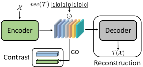
Figure 1: Conceptual illustration of proposed method. GO stands for global operations which convert feature maps to feature vectors. The blue feature vector comes from the momentum encoder. $vec(\mathcal{T})$ represents the indicator vector of $\mathcal{T}$ which contains a set of transformation functions. Each component in $vec(\mathcal{T})$ is 1 or 0 denoting whether the corresponding transformation is applied or not. $\odot$ stands for a channel-wise multiplication operation.

Nowadays, contrastive representation learning has been widely applied and outstandingly successful in medical image analysis [51, 33, 6]. The goal of contrastive learning is to learn invariant representations via contrasting medical image pairs, which can be regarded as an implicit way to preserve maximal information. Nonetheless, we think it is still beneficial and complemental to explicitly preserve more information in addition to the contrastive loss. To achieve this goal, an intuitive solution is to reconstruct the original inputs using learned representations so that these representations can preserve the information closely related to the inputs. However, we discover that directly adding a plain reconstruction branch for restoring the original inputs would not significantly improve the learned representations. To address this problem, we introduce Preservational Contrastive Representation Learning to reconstruct diverse contexts using representations learned from the contrastive loss.

As shown in Fig.1, we attempt to incorporate the diverse image reconstruction, as a pretext task, into contrastive learning. The main motivation is to encode more information into the learned representations. Specifically, we introduce Transformation-conditioned Attention and Cross-model Mixup to enrich the information carried by representations. The first module embeds a transformation indicator vector ($vec(\mathcal{T})$ in Figure 1) to high-level feature maps following an attentional mechanism. Based on the embedded vector, the network is required to dynamically reconstruct different image targets while the input is fixed. Cross-model Mixup is developed to generate a hybrid encoder by mixing the feature maps of the ordinary and the momentum encoders, where the hybrid encoder is asked to reconstruct mixed image targets. We show that both modules can help to encode more information and produce stronger representations compared to using contrastive learning only.

Besides the learning algorithm, this paper also addresses another issue when using unlabeled medical images for pretraining, that is lacking a fair and thorough comparison of different self-supervised learning methodologies. In this paper, we design extensive experiments to analyze the performance of different algorithms across different datasets and data modalities. Generally speaking, the contributions of this paper can be summarized into three aspects:

• Preservational Contrastive Representation Learning is introduced to encode more information into the representations learned from the contrastive loss by reconstructing diverse contexts.

• In order to restore diverse images, we propose two modules: Transformation-conditioned Attention and Cross-model Mixup to build a triple encoder, single decoder architecture for self-supervised learning.

• Extensive experiments and analyses show that the proposed PCRL has observable advantages in 5 classification/segmentation tasks, outperforming both self-supervised and supervised counterparts by substantial and significant margins.

2 Related Work

In this section, we mainly review deep model based self-supervised learning approaches and mixup strategies. Note that for self-supervised learning, we only list the most related ones based on pretext tasks, ignoring clustering based approaches [4, 47] and video based representation learning [38, 39, 28, 40].

Pretext-based self-supervised learning in natural images. Pretext-based methods rely on predicting input images’ properties that are covariant to the transformations, such as recognizing image patches’ content [29], relative position [14, 24], rotation degree [17, 14], object color [23, 46], the number of objects [25] and the applied transformation function [30]. Contrastive-estimation based approaches also utilize pretext tasks to learn invariant representations by contrasting image pairs [43, 26, 10, 5, 20, 48]. Recently, there are some works trying to remove the negative pairs in contrastive learning [18, 12]. By comparison, our method follows a different principle which is making representations able to fully describe their sources (i.e., corresponding input images).

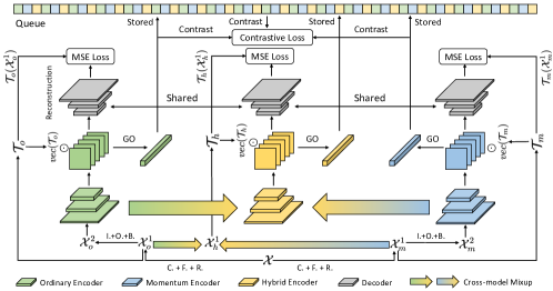
Figure 2: Overview of proposed framework. PCRL employs a U-Net like architecture to learn representations. For both encoder and decoder, we plot their feature maps for better demonstration. The hybrid encoder takes no input images as it consists of mixed feature maps from both the ordinary encoder and the momentum encoder. {C., F., R., I., O., B.} are abbreviations for random crop, random flip, random rotation, inpainting, outpainting and gaussian blur, respectively. NCE is short for noise-contrastive estimation. GO represents global operations which include global average pooling and fully-connected layers. $vec(\cdot)$ represents the indicator vector. $\mathcal{T}_{\{o,m,h\}}(\cdot)$ denote a set of transformation functions for different encoders. $\odot$ represents channel-wise multiplication. For simplicity, we do not plot the skip connections.

Self-supervised learning in medical image analysis. Before contrastive learning, solving the jigsaw problem [54, 53, 35] and reconstructing corrupted images [9, 52] are two major topics for pretext-based approaches in medical images. Besides them, Xie et al. [44] introduced a triplet loss for self-supervised learning in nuclei images. Haghighi et al. [19] improved [52] by appending a classification branch to classify the high-level features into different anatomical patterns. For contrastive learning, Zhou et al. [51] applied contrastive loss to 2D radiographs. Similar ideas have also appeared in few-shot [49] and semi-supervised learning [50]. Taleb et al. [34] proposed 3D Contrastive Predictive Coding from utilizing 3D medical images. There are two works [16, 8] most related to ours. Feng et al. [16] showed that the process of reconstructing part images displays similar effects with those of employing a contrastive loss. Chakraborty et al. [8] introduced a denoising autoencoder to capture a latent space representation. However, both methods failed to improve contrastive learning with context reconstruction while our methodology succeeds in this aspect.

Mixup in medical imaging. Mixup [45], as an augmentation strategy, has been widely adopted in medical imaging [27, 7, 22, 15, 2, 37]. The proposed Cross-model Mixup is most related to Manifold mixup [36, 22, 2]. However, as far as we know, there is no previous method applying manifold mixup to cross-model representations, which is exactly the core contribution of our Cross-model Mixup.

3 Methodology

An overview of Preservational Contrastive Representation Learning (PCRL) is provided in Figure 2. Generally, PCRL contains three different encoders and one shared decoder. The encoder and the decoder are connected via a U-Net like architecture. We first apply exponential moving average to the parameters of the ordinary encoder to produce the momentum encoder. Then, for each input, we apply Cross-model mixup to both encoders’ representations (feature maps) to build a hybrid encoder. Given a batch of images $\mathcal{X}$, we first apply random crop, random flip and random rotation to generate three batches of images $\mathcal{X}_{o}^{1}$, $\mathcal{X}_{m}^{1}$ and $\mathcal{X}_{h}^{1}$ for three different encoders, respectively. Then, we apply low-level processing operations, including inpainting, outpainting and gaussian blur, to each batch in order to generate the final inputs $\mathcal{X}_{\{o,m,h\}}^{2}$ for different encoders. In each training step, we randomly generate three sets of transformations (including flip and rotation): $\mathcal{T}_{o}$, $\mathcal{T}_{m}$ and $\mathcal{T}_{h}$ (please refer to Sec.3.1 for more details), and encode them into the last convolutional layer of each encoder. The ground truth targets of the MSE (mean square error) loss in image reconstruction are $\mathcal{T}_{o}(\mathcal{X}_{o}^{1})$, $\mathcal{T}_{m}(\mathcal{X}_{m}^{1})$ and $\mathcal{T}_{h}(\mathcal{X}_{h}^{1})$, corresponding to different encoders. For contrastive learning in PCRL, we introduce noise-contrastive estimation which stores past representations in a queue [20] and then apply contrastive loss to both positive and negative image pairs.

3.1 Transformation-conditioned Attention

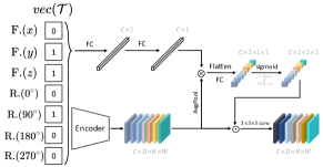
Figure 3: Our Transformation-conditioned Attention module. F. and R. stand for flip and rotation, respectively. {$x,y,z$} denote the axes. {0,$90\mathrm{°}$,$180\mathrm{°}$,$270\mathrm{°}$} denote the rotation degree. $vec(\mathcal{T})$ denotes the indicator vector of $\mathcal{T}$ whose subscript is omitted for simplicity. $\otimes$ means the outer product. $\odot$ represents the channel-wise multiplication. Note that the above figure demonstrates the implementation when each input is 3D. For 2D inputs, there is no F.($z$) in the indicator vector. For both 2D and 3D inputs, the rotation is only applied to the xy-plane.

In this section, we propose Transformation-conditioned Attention (TransAtt) to enable the reconstruction of diverse contexts. This module encodes the transformation vector into the high-level representations following an attentional mechanism. Such process can force the encoder to preserve more information in learned representations.

As shown in Figure 3, for each input, the indicator vector contains a combination of different transformations. Specifically, given 3D inputs (CT and MRI scans), the indicator vector has 7 components denoting different transformation strategies (cf. Figure 3). For 2D inputs (such as X-rays), the number of transformations decreases to 6 where F.($z$) does not exist. Each component contains an indicator function (1 or 0) representing whether the specific transformation is applied or not. To encode the indicator vector into high-level feature maps, we propose an attentional mechanism where we suppose that different channels of feature maps may have different impacts on the reconstructed results. Note that TransAtt is only applied to the last convolutional layer (before FC layers) of each encoder.

To imitate such process, we first forward the indicator vector $vec(\mathcal{T})$ to two fully-connected (FC) layers which produces a vector $f^{p}\in\mathbb{R}^{C\times 1}$. Meanwhile, we apply global average pooling to each encoder’s high-level feature maps $\mathcal{F}^{l}\in\mathbb{R}^{C\times D\times H\times W}$ resulting in a vector $f^{l}\in\mathbb{R}^{C\times 1}$, where $l$ denotes the layer index. Then, we compute the outer product of $f^{p}$ and $f^{l}$:

$$\begin{split}M=f^{p}\otimes f^{l},\end{split}$$ (1)

$M\in\mathbb{R}^{C\times C}$. Next, we flatten $M$ and forward it to another fully-connected layer:

$$\begin{split}f^{q}=\text{ReLU}\ (W_{\theta}\ \text{flat.}(M)),\end{split}$$ (2)

where $W_{\theta}\in\mathbb{R}^{C\times C^{2}}$ stands for the weight parameters of the FC layer. To perform rescaling, we further append a sigmoid function to $f^{q}$:

$$\begin{split}f^{w}=\text{sigmoid}(f^{q}),\end{split}$$ (3)

where $f^{w}\in\mathbb{R}^{C\times 1\times 1\times 1}$. Finally, we apply channel-wise multiplication between $\mathcal{F}^{l}$ and $f^{w}$ and append a convolutional layer whose kernel size is 3:

$$\begin{split}\mathcal{F}^{l+1}=\text{conv}(\mathcal{F}^{l}\odot f^{w}),\end{split}$$ (4)

where $\mathcal{F}^{l+1}\in\mathbb{R}^{C\times D\times H\times W}$.

3.2 Cross-model Mixup

Apart from TransAtt, we introduce Cross-model Mixup (CrossMix) for shuffling these feature representations in order to enable more diverse restoration. Different from traditional mixup [45] which applies to network inputs, we propose to mix the feature maps from two different models to build a new hybrid encoder.

Accordingly, the reconstruction target of the hybrid encoder is a mixed input $\mathcal{X}^{1}_{h}$. In practice, for each training iteration,

$$\begin{split}\mathcal{X}^{1}_{h}=\lambda\mathcal{X}^{1}_{o}+(1-\lambda)\mathcal{X}^{1}_{m},\end{split}$$ (5)

where $\lambda\sim\text{Beta}(\alpha,\alpha)$, $\alpha$ is a hyperparameter. For network feature maps, we use $\mathcal{F}^{i}_{o}$ to denote the feature maps at layer $i$ of the ordinary encoder, $i\in\{1,...,l\}$. Similarly, $\mathcal{F}^{i}_{m}$ and $\mathcal{F}^{i}_{h}$ stand for the features maps at the same location in the momentum encoder and the hybrid encoder, respectively. Thus, the process of cross-model representation mixup can be formulated as:

$$\begin{split}\mathcal{F}^{i}_{h}=\lambda\mathcal{F}^{i}_{o}+(1-\lambda)\mathcal{F}^{i}_{m}.\end{split}$$ (6)

Together with the one shared decoder, we can directly use $\mathcal{F}_{h}^{\{1,...,l\}}$ to reconstruct $\mathcal{T}_{h}(\mathcal{X}_{h}^{1})$.

3.3 Loss Functions and Model Update

To store past features for contrasting, we employ a queue $K=\{k_{1},...,k_{N}\}$ to store them following [20]. The length of $K$ is $N$. In contrastive learning, we treat all features in queue $K$ as negative samples. Here we use $g_{o}(\cdot)$ and $g_{m}(\cdot)$ to denote the projectors of the ordinary encoder and the momentum encoder, separately. The contrastive loss $\mathcal{L}_{c}$ can be formulated as:

$$\begin{split}\mathcal{L}_{c}=-\text{log}\frac{\exp([g_{o}(\mathcal{F}^{l+1}_{o})]^{T}g_{m}(\mathcal{F}^{l+1}_{m})/\tau)}{\sum_{j=1}^{N}\exp([g_{o}(\mathcal{F}^{l+1}_{o})]^{T}k_{j}/\tau)},\end{split}$$ (7)

where $\tau$ is a temperature hyperparameter. $g_{o}(\cdot)$ and $g_{m}(\cdot)$ contains global average pooling and two FC layers, independently. After each training iteration, we push $g_{o}(\mathcal{F}^{l+1}_{o})$, $g_{m}(\mathcal{F}^{l+1}_{m})$, and $g_{h}(\mathcal{F}^{l+1}_{h})$ to $K$ as negative samples for further contrasting.

For reconstructing diverse contexts, we use mean square error (MSE) as the default reconstruction loss. Formally, if we denote the shared decoder network as $D_{\theta}$, considering the whole network has a U-Net like architecture, the decoder’s inputs should be multi-layer feature maps $\mathcal{F}_{\{o,m,h\}}$. The computation of the reconstruction loss can be summarized as follows:

$$\small\begin{split}\mathcal{L}_{p}&=\text{MSE}(D_{\theta}(\mathcal{F}_{o}),\ \mathcal{T}_{o}(\mathcal{X}_{o}^{1}))+\text{MSE}(D_{\theta}(\mathcal{F}_{m}),\ \mathcal{T}_{m}(\mathcal{X}_{m}^{1}))\\ &\ \ \ \ \ +\text{MSE}(D_{\theta}(\mathcal{F}_{h}),\ \mathcal{T}_{h}(\mathcal{X}_{h}^{1})).\end{split}$$ (8)

We finally sum up $\mathcal{L}_{c}$ and $\mathcal{L}_{p}$ as the complete loss function with equal weight (0.5 to 0.5). For network parameters, we denote the parameters of the ordinary encoder and the momentum encoder as $\theta_{o}$ and $\theta_{m}$, respectively. We update $\theta_{m}$ by using an exponential moving average (EMA) factor $\beta$:

$$\begin{split}\theta_{m}=\beta\theta_{m}+(1-\beta)\theta_{o}.\end{split}$$ (9)

Note that the hybrid encoder has no encoder parameters as it directly takes a combination of the feature maps from the ordinary and the momentum encoders. The mixed feature maps are then treated as the inputs to the shared decoder as shown in Equation 8.

4 Experiments

In this section, we first make ablation studies to demonstrate the advantages of TransAtt and CrossMix. Then, we introduce a thorough analysis of different self-supervised algorithms from different aspects. For all tasks, we employ the notation of source dataset$\rightarrow$target dataset. The source dataset is used for self-supervised pretraining while the target dataset is used for supervised finetuning.

4.1 Baselines

For medical pretraining approaches, we divide them into two categories: 2D and 3D, simply based on their input dimension (e.g., X-ray is 2D while CT scan is 3D). For 2D image pretraining, our baselines include train from scratch (TS), ImageNet pretraining (IN), Model Genesis (MG) [52], Semantic Genesis (SG) [19] and Comparing to Learn (C2L) [51]. Here we ignore the method proposed in [44] which made prior assumptions on the number of nuclei and is not be suitable for other datasets. For 3D volume pretraining, we also include train from scratch (TS), Model Genesis (MG), Semantic Genesis (SG) and 3D-CPC [34]. Additionally, Cube++ [35] is included as it is an improved version of Rubik’s Cube [54] and Rubik’s Cube+ [53].

4.2 Datasets

In 2D tasks, we make experiments on two X-ray datasets: Chest14 [41] and CheXpert [21]. We use Chest14 for both 2D pretraining and 2D finetuning while CheXpert is only used for pretraining considering CheXpert contains a number of uncertain labels. The evaluation metric in 2D tasks is AUC. In order to evaluate the performance of algorithms on 3D volumes, we make experiments on CT and MRI datasets, including LUNA [32], BraTS [1] and LiTS [3]. We use LUNA for both 3D pretraining and 3D finetuning. The evaluation metric of finetuning on LUNA is AUC. BraTS is only used for supervised finetuning to test the cross-modal transferability following [52]. LiTS is mainly used for 3D finetuning on liver segmentation. The evaluation metric for segmentation is mean dice score. In practice, we divide each dataset into the training set, the validation set and the test set. The pretraining data always come from the training set (without labels). Please refer to the supplementary material for more details.

4.3 Implementation Details

We use 2D U-Net [31] and 3D U-Net [13] as the backbone networks for 2D and 3D tasks, where we replace the encoder in 2D U-Net with ResNet-18. The EMA factor $\beta$ of updating momentum encoder is set to 0.99. For self-supervised pretraining, we employ momentum SGD as the default optimizer whose initial learning rate is set to 1e-3 while the momentum value is set to 0.9. We employ the cosine annealing strategy for decreasing learning rate and stop the training when the validation loss does not change for 30 epochs. The checkpoints with lowest validation loss values are saved for finetuning. For supervised finetuning, we use Adam as the optimizer with 1e-4 as the initial learning rate. Similar to pretraining, we rely on validation loss to determine when to end the training stage, and we save the checkpoints with lowest validation loss values for testing. Dice loss is used for segmentation tasks while cross entropy is employed for classification tasks. For other hyperparameters in baselines, we simply follow the choices in their official papers. $\alpha$ is set to 1 (for $\lambda$) in both Equation 5 and 6. We set the temperature factor $\tau$ of softmax function in Equation 7 to 0.2 in practice. For each experiment, we repeat it for three times and report their average results. More details can be found in attached supplementary material.

4.4 Ablation Study

Method	Pretext Task
	Rotation [17]	Position [14]
ContraLoss	85.5	82.3
ContraLoss + Self-Recons.	87.9	84.5
ContraLoss + TransAtt (Flip)	89.2	86.4
ContraLoss + TransAtt	91.0	89.3
ContraLoss + CrossMix	90.5	88.3
PCRL (All modules)	93.2	91.6

Table 1: Investigation of whether our method contains more information. ContraLoss stands for the contrastive loss. Self-Recons. represents self-reconstruction which is reconstructing the input images without any variations. Acc. stands for the classification accuracy. TransAtt (Flip) means that the indicator function in TransAtt only contains the flip operation.

Method	Chest14$\rightarrow$Chest14
	9:1	8:2
ContraLoss	71.7	74.8
ContraLoss + Self-Recons.	72.5	75.4
ContraLoss + RotNet	72.3	75.2
ContraLoss + TransAtt (Flip)	73.5	76.6
ContraLoss + TransAtt	74.4	77.4
ContraLoss + CrossMix ($\alpha$=0.5)	73.3	76.1
ContraLoss + CrossMix ($\alpha$=1)	73.7	76.6
PCRL (All modules)	76.2	78.8

Table 2: Investigation of different module combinations. In Chest14$\rightarrow$Chest14, 9:1 demonstrates that we use 90% data for self-supervised pretraining while the rest 10% are used for finetuning. RotNet represents that we replace Self-Recons. with the task of rotation prediction.

Method	Chest14$\rightarrow$Chest14					CheXpert$\rightarrow$Chest14
	9.5:0.5	9:1	8:2	7:3	6:4	10%	20%	30%	40%	50%	60%	100%
TS	61.8	68.1	71.5	73.4	75.4	68.1	71.5	73.4	75.4	77.5	79.1	80.9
IN	70.5	73.6	75.3	76.9	78.0	73.5	76.3	78.4	79.0	79.5	79.7	81.0
MG	66.4	70.0	73.9	76.1	77.3	70.1	73.9	75.5	76.5	77.6	79.3	80.8
SG	66.5	70.2	74.3	76.7	77.6	69.7	73.8	75.6	77.3	77.3	79.6	81.3
C2L	71.7	74.1	76.4	77.5	79.0	73.1	77.0	78.5	79.1	79.8	80.2	81.5
PCRL	74.1	76.2	78.8	79.0	79.9	75.8	77.6	79.8	80.8	81.2	81.7	83.1
p-value	5.2e-4	9.6e-4	2e-3	1.8e-3	2.3e-3	2.4e-3	8.1e-4	2.4e-3	3.5e-4	5.6e-4	3.6e-3	2.7e-3

(a) 2D tasks: pretraining using Chest14 or CheXpert

Method	LUNA$\rightarrow$LUNA				LUNA$\rightarrow$LiTS					LUNA$\rightarrow$BraTS
	9:1	8:2	7:3	6:4	10%	20%	30%	40%	100%	10%	20%	30%	40%	100%
TS	78.4	83.0	85.7	87.5	71.1	77.2	84.1	87.3	90.7	66.6	72.7	76.7	77.1	81.5
MG	80.2	85.0	87.5	90.3	73.3	79.5	84.3	87.9	91.3	69.6	75.5	79.6	80.4	82.4
Cube++	81.4	85.2	87.9	90.0	74.2	79.3	84.5	88.2	91.8	69.0	74.9	79.3	79.7	82.2
SG	79.3	84.5	87.9	90.5	73.8	79.3	85.5	88.2	91.4	70.3	75.6	79.1	80.8	82.3
3D-CPC	80.2	85.2	88.3	90.6	74.8	80.2	85.6	88.9	91.9	70.1	75.9	79.4	81.2	82.9
PCRL	84.4	87.5	89.8	92.2	77.3	83.5	87.8	90.1	93.7	71.6	77.6	81.1	83.3	85.0
p-value	7.5e-4	1.5e-3	2.1e-3	1.9e-3	2e-3	1.7e-3	9e-4	2.5e-3	2.4e-4	8.4e-4	3.5e-3	5.7e-3	2.5e-3	2.4e-3

(b) 3D tasks: pretraining using LUNA

Figure 4: Comparison of different methods. In (a), we report the results of 2D tasks. In (b), the results of 3D tasks are displayed. The ratios in Chest14$\rightarrow$Chest14 and LUNA$\rightarrow$LUNA stand for the amount of unlabeled data (for pretraining) with respect to the amount of labeled data (for finetuning). In other tasks, the ratios represent the amount of data of the source dataset used for pretraining. For experiments of LiTS, we report the dice score of liver segmentation. For BraTS, we compute the mean dice of whole tumor, tumor core and enhancing tumor. We also report the p-values between the best and the second best results for each ratio to demonstrate the significance of PCRL.

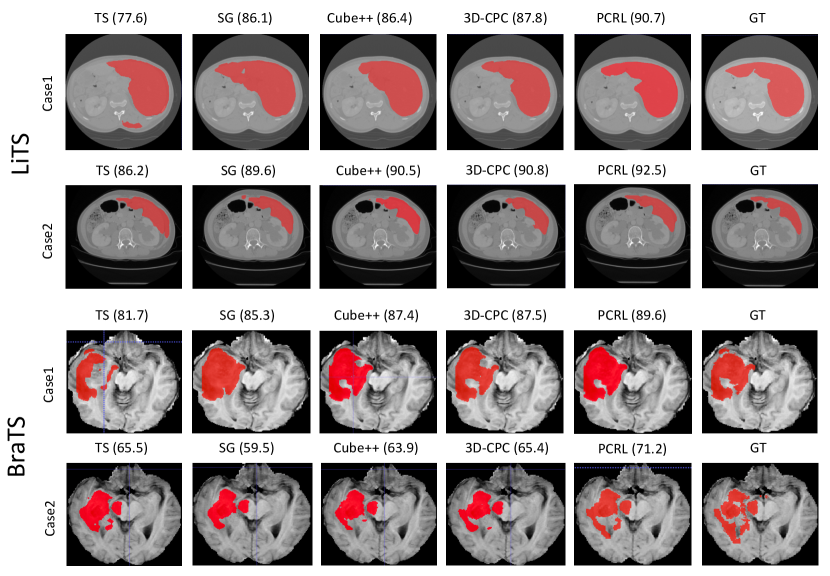
Figure 5: Visual analysis of segmentation results when finetuning on LiTS and BraTS. For each dataset, we provide 2 cases where we report the dice scores using different self-supervised pretraining methodologies. Specifically, in LiTS, the goal is to segment liver. In BraTS, we only display the results of WT. We ignore MG because SG is built on top of MG.

In this section, we mainly investigate two problems: 1) whether the proposed method preserves more information than contrastive learning (Table 1) and 2) if the preserved information lead to the improved performance (Table 2). In Table 2, we make experiments on Chest14 to investigate the effectiveness of different module combinations, where we treat different ratios of the dataset as labeled data for supervised finetuning while the rest are used as unlabeled data for self-supervised pretraining.

Preservational learning brings more information to representations. In Table 1, we show that reconstructing diverse contexts does bring more information in learned representations. We introduce two pretext tasks: predicting the rotation degree [17] and the relative position between images patches [14] to evaluate the amount of information in representations. In practice, we fixed the pretrained models as feature extractors and finetune the last fully connected layer for pretext tasks. Note that we directly utilize the pretrained models in CheXpert and use Chest14 to conduct pretext tasks. Specifically, when predicting the relative position between two image patches, we first divide the original input image to 14$\times$14 patches. Then, we extract adjacent image patches and formalize the position prediction problem as a 8-class classification problem (top, top left, top right, left, right, bottom left, bottom, bottom right). Similarly, when predicting the rotation degree, we manually rotate each input image by a specific degree and train the network to predict this degree, which can also be converted to a classification problem following [17]. We display the classification results in Table 1. It is obvious that ContraLoss + Self-Recons. can already perform better than using ContraLoss only by preserving more information obtained from simply reconstructing the original input images. More importantly, the proposed TransAtt module outperforms Self-Recons. by only employing the flip operation. Together with the rotation transformations, TransAtt greatly surpasses Self-Recons. on both pretext tasks, which demonstrates that TransAtt is able to preserve much more information than reconstructing the original input images. Similar phenomena can also be observed when applying CrossMix. Finally, PCRL achieves much higher accuracy than the others, again verifying reconstructing diverse contexts do help preserve more information in learned features.

Preserved information lead to better performance. We report the performance of different module combinations in Table 2, where we can observe similar trends as those in Table 1. It is obvious that the results on pretext tasks are closely correlated with the performance on Chest14. In other words, given a method, we can rely on its performance on two pretext tasks to roughly predict its performance in Chest14. Considering the performance on two pretext tasks can reflect the amount of information in learned representations, we can easily draw a conclusion: reconstructing diverse contexts introduce more information which help improve the overall performance of algorithms.

From Table 2, we can easily find that adding a self-reconstruction branch only brings marginal improvements over the baseline model. Similar phenomena can also be observed when we replace Self-Recons. with RotNet [17]. These results show that the contrastive loss already captures the information about simple pretext tasks without directly implementing these tasks. The fact that Self-Recons. performs better than RotNet shows that image reconstruction can preserve more information than RotNet. As for TransAtt, by comparing TransAtt (Flip) with TransAtt, we find that adding the rotation transformations can obviously improve the overall performance. This is consistent with the results in Table 1, where TransAtt also performs better than TransAtt (Flip) on two pretext tasks. We also investigate the influence of the hyperparameter $\alpha$ in CrossMix. The observation is that by decreasing its value by half, the overall performance slightly drops. Equipped with TransAtt and CrossMix, PCRL can surpass the baseline model ContraLoss by approximate 4 points in different labeled ratios. Moreover, we find that the improvement is most significant at 10%. This phenomenon implies that the reconstructing diverse contexts is more useful when the amount of labeled data is small.

4.5 Comparison with State-of-the-Arts in 2D Tasks

In this part, we evaluate the performance of various self-supervised pretraining approaches on 2 different 2D tasks: Chest14$\rightarrow$Chest14 and CheXpert$\rightarrow$Chest14. All results are displayed in Table 4a.

If we look at the results in Chest14$\rightarrow$Chest14, it is obvious that all pretraining methods (including IN) can boost the performance apparently when compared to TS. We can see that MG and SG achieve similar performance in different ratios. Such comparison is easy to explain as SG is built upon MG. However, both MG and SG still cannot surpass IN especially when the amount of labeled data is limited, which demonstrates that being pretrained on a large-scale natural image dataset can benefit medical image analysis a lot. As for C2L, we find that C2L is the only baseline method which is able to surpass IN in different ratios. When we compare PCRL with other baseline algorithms, it is easy to find that PCRL has the ability to outperform different baselines in various ratios significantly. Particularly, PCRL seems to have more advantages in small labeled ratios. The underlying reason may be that TransAtt and CrossMix may help to learn more diversified representations and alleviate the overfitting problem of training deep neural networks with limited supervision.

In CheXpert$\rightarrow$Chest14, we can see that MG and SG achieve comparable results with TS when the labeled ratio is equal or greater than 50%, demonstrating purely pretext-based approaches may have unstable performance under varying labeled ratios. If we look at C2L, we can find that C2L consistently outperforms IN and other pretraining methods in almost all ratios. Somewhat surprisingly, we find that PCRL can still outperform C2L and IN by a significant margin even if the labeled ratio is 100%. Such comparison further demonstrates the robustness of PCRL.

Method	#. Epoch	Cityscapes	COCO
SimCLR [9]	1000	75.6	39.6
SwAV [4]	400	76.0	-
MoCov2[11]	800	76.3	40.5
PCRL	800	77.3	41.3

Table 3: Results in natural images. We transfer the self-supervised pretrained models on ImageNet-1k to downstream tasks, including segmentation (Cityscapes) and detection (COCO). On Cityscapes, we use ResNet-50 as backbone to build a FCN segmentation model where the evaluation metric is mIoU. On COCO, we use the ResNet-50-FPN model from Detectron2 [42] and the evaluation metric is mAP (0.5:0.05:0.95).

4.6 Comparison with State-of-the-Arts in 3D Tasks

Besides 2D tasks, we also analyze the results of 3D self-supervised learning approaches in 3 different 3D tasks: LUNA$\rightarrow$LUNA, LUNA$\rightarrow$LiTS and LUNA$\rightarrow$BraTS, where all experimental results are shown in Table 4b.

In LUNA$\rightarrow$LUNA, it is interesting to find that the performance gaps between TS and self-supervised pretraining are smaller than those in Chest14. One explanation is that the nodule classification task is less sensitive to the amount of labeled data. Among MG, SG, Cube++ and 3D-CPC, 3D-CPC gives the best results in large labeled ratios while Cube++ performs better in small ones. Interestingly, as the labeled ratio increases, SG quickly catches up with MG and Cube++, showing its ability to utilize a large number of labeled images. Again, we can see that PCRL is able to outperform other baselines significantly in different ratios. Particularly, when the baseline approaches show similar results as the labeled ratio becomes larger, PCRL can still display impressive improvements over previous self-supervised pretraining approaches and outperforms TS substantially. In LUNA$\rightarrow$LiTS, Cube++ performs slightly better than MG and SG while 3D-CPC outperforms Cube++ in allmost all ratios. By comparison, PCRL has apparent advantages over other baselines especially when the labeled ratio is smaller or equal to 50%.

When we transfer knowledge from LUNA to BraTS, MG, SG and Cube++ display similar performance, all surpassing TS significantly in different labeled ratios. Due to advantages of contrastive learning, 3D-CPC again outperforms other baselines. Meanwhile, PCRL once again surpasses previous baselines consistently and remarkably. We think that such significant improvements can be attributed to the incorporation of the reconstruction of diverse contexts.

4.7 Visual Analysis

In Figure 5, we provide comparative visual analysis results of segmentation tasks in LiTS and BraTS, where the samples are randomly selected. We can obviously observe that PCRL handles the details much better than those of other baselines. For instance, in the first example of LiTS, PCRL delineates the corners accurately. In the second example of BraTS, PCRL can detect the isolated tumor regions while other methods cannot well handle these difficult cases.

4.8 Comparison with State-of-the-Arts in Natural Image Segmentation and Detection Tasks

To investigate the performance of PCRL in natural images, we conduct pretraining tasks on ImageNet-1k and transfer the pretrained models to downstream segmentation and detection tasks. The results are displayed in Table 3. We can see that PCRL is able to outperform MoCov2 and other popular self-supervised learning methods substantially in both Cityscapes and COCO, which are two widely adopted datasets in segmentation and detection. The superior performance on Cityscapes and COCO again verify the advantages of incorporating diverse context reconstruction.

5 Discussion and Conclusion

We show that by reconstructing diverse contexts, the learned representations using the contrastive loss can be greatly improved in medical image analysis. Our approach has shown positive results of self-supervised learning in a variety of medical tasks and datasets. There are some questions worth further discussing and verifying. For example, is preserving more information the only reason leading to the improvements over the contrastive loss? We hope the proposed PCRL can lay the foundations for real-world medical imaging tasks.

6 Acknowledgements

This work and the related project were funded in part by National Key Research and Development Program of China (No.2019YFC0118101), National Natural Science Foundation of China (No.81971616), Zhejiang Province Key Research & Development Program (No.2020C03073), National Natural Science Foundation of China (No.61931024) and the Guangdong Provincial Key Laboratory of Big Data Computing, The Chinese University of Hong Kong, Shenzhen.

7 Thorough Implementation Details (Supplementary Material)

In each dataset, we build the training set, the validation set and the test set using 70%, 10% and 20% of the whole dataset, respectively. Particularly, if a dataset is used for self-supervised pretraining and supervised finetuning in a semi-supervised manner, we construct the training set of pretraining by extracting a specific amount of data from the complete training set while the rest of the training set are used for finetuning. More details will be introduced in the following.

• Chest14 [41] is comprised of 112,120 X-ray images with 14 diseases from 30,805 unique patients. Each input image is resized to 224$\times$224 after random crop. In our experiments, Chest14 is used for both 2D pretraining and 2D finetuning. The batch size of pretraining is 256 and the batch size of finetuning is 512, where we use batch normalization for all experiments. The evaluation metric of finetuning is AUC.

• CheXpert [21] is a large public dataset for chest radiograph interpretation, consisting of 224,316 chest radiographs of 65,240 patients. Each input image is resized to 224$\times$224 after random crop. Considering CheXpert contains uncertain labels, we mainly use CheXpert for 2D pretraining. The batch size of pretraining is 256 and we use batch normalization for all experiments.

• LUNA [32] contains 888 CT scans with lung nodule annotations. Note that LUNA has different preprocessing strategies for different approaches which will be clarified in the following. We use LUNA for both 3D pretraining and 3D finetuning. The evaluation metric of finetuning is AUC. The range of the Hounsfield Units (HU) is [-1000,1000]. The batch size of pretraining and finetuning is 32 and we use batch normalization in all experiments.

• BraTS [1] includes 351 MRI scans of brain tumor (in 2018 challenge). BraTS shares similar preprocessing strategies with those of LUNA. We use BraTS for 3D finetuning. The evaluation metric of finetuning is dice score. Since the batch size is 4 for all finetuning experiments, we use group normalization to replace batch normalization in the pretrained models.

• LiTS [3] contains 131 available CT scans with their annotations for liver and tumor. LiTS is mainly used for 3D finetuning where we first localize the liver and expand the target volume by 30 slices in each axis. The segmentation target is liver only. The input size is 256$\times$256$\times$64 after random crop. Dice coefficient is employed as the evaluation metric while the range of HU is [-200,200]. The batch size is 4. Similar to BraTS, we also use group normalization to replace batch normalization in the pretrained models.

For network architectures, in Chest14$\rightarrow$Chest14 and CheXpert$\rightarrow$Chest14, we simply follow [51, 33] to conduct experiments based on ResNet-18. In 3D tasks, we directly use the ordinary 3D U-Net as backbone. We will demonstrate the implementation details of each approach in the following.

• MG [52]. In LUNA and BraTS datasets, we apply random crop to produce each input tensor whose size is 64$\times$64$\times$32 (corresponding to x, y and z axes). The augmentation strategies on all datasets include patch shuffling, non-linear transformation, inpainting, outpainting and random flip.

• SG [19]. Similar to MG, we apply random crop to generate 64$\times$64$\times$32 patches in LUNA and BraTS datasets. For the number of nearest neighbors, we set it to 200/1000 in 3D and 2D tasks, respectively. Note that SG follows similar augmentation strategies used in MG.

• Cube++ [35]. Similar to MG and SG, the input size is 64$\times$64$\times$32 in LUNA and BraTS datasets. Then, we divide each volume into 32 subvolumes. The size of each subvolume is 16$\times$16$\times$16. We then apply random rotation to each subvolume and employs a generative neural network to reconstruct the original input volume.

• C2L [51]. Give a 2D input image, we apply random crop, flip, rotation (10 degree) and grayscale to generate random patches. For each patch, we resize it to 224$\times$224 and apply inpainting to it.

• 3D-CPC [13]. We follow the instructions in [13] to implement a 3D-CPC model.

• PCRL. The augmentation strategies include random crop, random flip, random rotation, inpainting, outpainting and gaussian blur. For 2D images, we simply apply these operations to generate two input patches. Specially, for each 3D input, we randomly crop 16 pairs of volumetric inputs. The two volumes in each pair have the same size which is randomly sampled from {64$\times$64$\times$32, 96$\times$96$\times$48, 96$\times$96$\times$96, 32$\times$32$\times$16, 112$\times$112$\times$56}. Note that we require the Interaction over Union (IoU) within each pair to be larger than 0.2. Finally, we resample each volume to 64$\times$64$\times$32. Note that random rotation is only applied to xy-plane in 3D volume where the maximum degree is $10\mathrm{°}$. The length of queue which stores past representations is 16384 in PCRL. Note that the reason why we do not use online random crop in 3D images is that the computational cost of such operation (including crop and resize) is somewhat unacceptable in our GPU device. For both 2D and 3D tasks, we take 4 NVIDIA TITAN V GPUs to train PCRL models. The pretraining tasks on Chest14 and LUNA take 1 day and a half day, respectively.

References

- [1] Spyridon Bakas, Mauricio Reyes, Andras Jakab, Stefan Bauer, Markus Rempfler, Alessandro Crimi, Russell Takeshi Shinohara, Christoph Berger, Sung Min Ha, Martin Rozycki, et al. Identifying the Best Machine Learning Algorithms for Brain Tumor Segmentation, Progression Assessment, and Overall Survival Prediction in the BRATS Challenge. arXiv preprint arXiv:1811.02629, 2018.
- [2] Tariq Bdair, Nassir Navab, and Shadi Albarqouni. ROAM: Random Layer Mixup for Semi-Supervised Learning in Medical Imaging. arXiv preprint arXiv:2003.09439, 2020.
- [3] Patrick Bilic, Patrick Ferdinand Christ, Eugene Vorontsov, Grzegorz Chlebus, Hao Chen, Qi Dou, Chi-Wing Fu, Xiao Han, Pheng-Ann Heng, Jürgen Hesser, et al. The Liver Tumor Segmentation Benchmark (LiTS). arXiv preprint arXiv:1901.04056, 2019.
- [4] Mathilde Caron, Piotr Bojanowski, Armand Joulin, and Matthijs Douze. Deep Clustering for Unsupervised Learning of Visual Features. In Proceedings of the European Conference on Computer Vision (ECCV), pages 132–149, 2018.
- [5] Mathilde Caron, Ishan Misra, Julien Mairal, Priya Goyal, Piotr Bojanowski, and Armand Joulin. Unsupervised Learning of Visual Features by Contrasting Cluster Assignments. arXiv preprint arXiv:2006.09882, 2020.
- [6] Krishna Chaitanya, Ertunc Erdil, Neerav Karani, and Ender Konukoglu. Contrastive Learning of Global and Local Features for Medical Image Segmentation with Limited Annotations. arXiv preprint arXiv:2006.10511, 2020.
- [7] Krishna Chaitanya, Neerav Karani, Christian F Baumgartner, Anton Becker, Olivio Donati, and Ender Konukoglu. Semi-supervised and Task-driven Data Augmentation. In International Conference on Information Processing in Medical Imaging, pages 29–41. Springer, 2019.
- [8] Souradip Chakraborty, Aritra Roy Gosthipaty, and Sayak Paul. G-SimCLR: Self-Supervised Contrastive Learning with Guided Projection via Pseudo Labelling. arXiv preprint arXiv:2009.12007, 2020.
- [9] Liang Chen, Paul Bentley, Kensaku Mori, Kazunari Misawa, Michitaka Fujiwara, and Daniel Rueckert. Self-supervised Learning for Medical Image Analysis using Image Context Restoration. Medical Image Analysis, 58:101539, 2019.
- [10] Ting Chen, Simon Kornblith, Mohammad Norouzi, and Geoffrey Hinton. A Simple Framework for Contrastive Learning of Visual Representations. arXiv preprint arXiv:2002.05709, 2020.
- [11] Xinlei Chen, Haoqi Fan, Ross Girshick, and Kaiming He. Improved Baselines with Momentum Contrastive Learning. arXiv preprint arXiv:2003.04297, 2020.
- [12] Xinlei Chen and Kaiming He. Exploring Simple Siamese Representation Learning. arXiv preprint arXiv:2011.10566, 2020.
- [13] Özgün Çiçek, Ahmed Abdulkadir, Soeren S Lienkamp, Thomas Brox, and Olaf Ronneberger. 3D U-Net: Learning Dense Volumetric Segmentation from Sparse Annotation. In International Conference on Medical Image Computing and Computer-Assisted Intervention, pages 424–432. Springer, 2016.
- [14] Carl Doersch, Abhinav Gupta, and Alexei A Efros. Unsupervised Visual Representation Learning by Context Prediction. In Proceedings of the IEEE International Conference on Computer Vision, pages 1422–1430, 2015.
- [15] Zach Eaton-Rosen, Felix Bragman, Sebastien Ourselin, and M Jorge Cardoso. Improving Data Augmentation for Medical Image Segmentation. Medical Imaging with Deep Learning, 2018.
- [16] Zeyu Feng, Chang Xu, and Dacheng Tao. Self-supervised Representation Learning by Rotation Feature Decoupling. In Proceedings of the IEEE Conference on Computer Vision and Pattern Recognition, pages 10364–10374, 2019.
- [17] Spyros Gidaris, Praveer Singh, and Nikos Komodakis. Unsupervised Representation Learning by Predicting Image Rotations. arXiv preprint arXiv:1803.07728, 2018.
- [18] Jean-Bastien Grill, Florian Strub, Florent Altché, Corentin Tallec, Pierre H Richemond, Elena Buchatskaya, Carl Doersch, Bernardo Avila Pires, Zhaohan Daniel Guo, Mohammad Gheshlaghi Azar, et al. Bootstrap Your Own Latent: A New Approach to Self-supervised Learning. arXiv preprint arXiv:2006.07733, 2020.
- [19] Fatemeh Haghighi, Mohammad Reza Hosseinzadeh Taher, Zongwei Zhou, Michael B Gotway, and Jianming Liang. Learning Semantics-enriched Representation via Self-discovery, Self-classification, and Self-restoration. In International Conference on Medical Image Computing and Computer-Assisted Intervention, pages 137–147. Springer, 2020.
- [20] Kaiming He, Haoqi Fan, Yuxin Wu, Saining Xie, and Ross Girshick. Momentum Contrast for Unsupervised Visual Representation Learning. In Proceedings of the IEEE/CVF Conference on Computer Vision and Pattern Recognition, pages 9729–9738, 2020.
- [21] Jeremy Irvin, Pranav Rajpurkar, Michael Ko, Yifan Yu, Silviana Ciurea-Ilcus, Chris Chute, Henrik Marklund, Behzad Haghgoo, Robyn Ball, Katie Shpanskaya, et al. CheXpert: A Large Chest Radiograph Dataset with Uncertainty Labels and Expert Comparison. In Proceedings of the AAAI Conference on Artificial Intelligence, volume 33, pages 590–597, 2019.
- [22] Wonmo Jung, Sejin Park, Kyu-Hwan Jung, and Sung Il Hwang. Prostate Cancer Segmentation using Manifold Mixup U-Net. In International Conference on Medical Imaging with Deep Learning–Extended Abstract Track, 2019.
- [23] Gustav Larsson, Michael Maire, and Gregory Shakhnarovich. Learning Representations for Automatic Colorization. In European conference on computer vision, pages 577–593. Springer, 2016.
- [24] Mehdi Noroozi and Paolo Favaro. Unsupervised Learning of Visual Representations by Solving Jigsaw Puzzles. In European Conference on Computer Vision, pages 69–84. Springer, 2016.
- [25] Mehdi Noroozi, Hamed Pirsiavash, and Paolo Favaro. Representation Learning by Learning to Count. In Proceedings of the IEEE International Conference on Computer Vision, pages 5898–5906, 2017.
- [26] Aaron van den Oord, Yazhe Li, and Oriol Vinyals. Representation Learning with Contrastive Predictive Coding. arXiv preprint arXiv:1807.03748, 2018.
- [27] Egor Panfilov, Aleksei Tiulpin, Stefan Klein, Miika T Nieminen, and Simo Saarakkala. Improving Robustness of Deep Learning based Knee MRI Segmentation: Mixup and Adversarial Domain Adaptation. In Proceedings of the IEEE/CVF International Conference on Computer Vision Workshops, pages 0–0, 2019.
- [28] Deepak Pathak, Ross Girshick, Piotr Dollár, Trevor Darrell, and Bharath Hariharan. Learning Features by Watching Objects Move. In Proceedings of the IEEE Conference on Computer Vision and Pattern Recognition, pages 2701–2710, 2017.
- [29] Deepak Pathak, Philipp Krahenbuhl, Jeff Donahue, Trevor Darrell, and Alexei A Efros. Context encoders: Feature learning by inpainting. In Proceedings of the IEEE conference on computer vision and pattern recognition, pages 2536–2544, 2016.
- [30] Guo-Jun Qi, Liheng Zhang, Feng Lin, and Xiao Wang. Learning Generalized Transformation Equivariant Representations via Autoencoding Transformations. IEEE Transactions on Pattern Analysis and Machine Intelligence, 2020.
- [31] Olaf Ronneberger, Philipp Fischer, and Thomas Brox. U-Net: Convolutional Networks for Biomedical Image Segmentation. In International Conference on Medical Image Computing and Computer-Assisted Intervention, pages 234–241. Springer, 2015.
- [32] Arnaud Arindra Adiyoso Setio, Alberto Traverso, Thomas De Bel, Moira SN Berens, Cas van den Bogaard, Piergiorgio Cerello, Hao Chen, Qi Dou, Maria Evelina Fantacci, Bram Geurts, et al. Validation, Comparison, and Combination of Algorithms for Automatic Detection of Pulmonary Nodules in Computed Tomography Images: the LUNA16 Challenge. Medical image analysis, 42:1–13, 2017.
- [33] Hari Sowrirajan, Jingbo Yang, Andrew Y Ng, and Pranav Rajpurkar. MoCo Pretraining Improves Representation and Transferability of Chest X-ray Models. arXiv preprint arXiv:2010.05352, 2020.
- [34] Aiham Taleb, Winfried Loetzsch, Noel Danz, Julius Severin, Thomas Gaertner, Benjamin Bergner, and Christoph Lippert. 3D Self-supervised Methods for Medical Imaging. arXiv preprint arXiv:2006.03829, 2020.
- [35] Xing Tao, Yuexiang Li, Wenhui Zhou, Kai Ma, and Yefeng Zheng. Revisiting Rubik’s Cube: Self-supervised Learning with Volume-wise Transformation for 3D medical Image Segmentation. In International Conference on Medical Image Computing and Computer-Assisted Intervention, pages 238–248. Springer, 2020.
- [36] Vikas Verma, Alex Lamb, Christopher Beckham, Amir Najafi, Ioannis Mitliagkas, David Lopez-Paz, and Yoshua Bengio. Manifold Mixup: Better Representations by Interpolating Hidden States. In International Conference on Machine Learning, pages 6438–6447. PMLR, 2019.
- [37] Dong Wang, Yuan Zhang, Kexin Zhang, and Liwei Wang. FocalMix: Semi-supervised Learning for 3D Medical Image Detection. In Proceedings of the IEEE/CVF Conference on Computer Vision and Pattern Recognition, pages 3951–3960, 2020.
- [38] Xiaolong Wang and Abhinav Gupta. Unsupervised Learning of Visual Representations using Videos. In Proceedings of the IEEE International Conference on Computer Vision, pages 2794–2802, 2015.
- [39] Xiaolong Wang, Kaiming He, and Abhinav Gupta. Transitive invariance for self-supervised visual representation learning. In Proceedings of the IEEE International Conference on Computer Vision, pages 1329–1338, 2017.
- [40] Xiaolong Wang, Allan Jabri, and Alexei A Efros. Learning Correspondence from the Cycle-consistency of Time. In Proceedings of the IEEE Conference on Computer Vision and Pattern Recognition, pages 2566–2576, 2019.
- [41] Xiaosong Wang, Yifan Peng, Le Lu, Zhiyong Lu, Mohammadhadi Bagheri, and Ronald M Summers. ChestX-ray8: Hospital-scale Chest X-ray Database and Benchmarks on Weakly-supervised Classification and Localization of Common Thorax Diseases. In Proceedings of the IEEE Conference on Computer Vision and Pattern Recognition, pages 2097–2106, 2017.
- [42] Yuxin Wu, Alexander Kirillov, Francisco Massa, Wan-Yen Lo, and Ross Girshick. Detectron2. https://github.com/facebookresearch/detectron2, 2019.
- [43] Zhirong Wu, Yuanjun Xiong, Stella X Yu, and Dahua Lin. Unsupervised Feature Learning via Non-parametric Instance Discrimination. In Proceedings of the IEEE Conference on Computer Vision and Pattern Recognition, pages 3733–3742, 2018.
- [44] Xinpeng Xie, Jiawei Chen, Yuexiang Li, Linlin Shen, Kai Ma, and Yefeng Zheng. Instance-Aware Self-supervised Learning for Nuclei Segmentation. In International Conference on Medical Image Computing and Computer-Assisted Intervention, pages 341–350. Springer, 2020.
- [45] Hongyi Zhang, Moustapha Cisse, Yann N Dauphin, and David Lopez-Paz. Mixup: Beyond Empirical Risk Minimization. arXiv preprint arXiv:1710.09412, 2017.
- [46] Richard Zhang, Phillip Isola, and Alexei A Efros. Split-brain Autoencoders: Unsupervised Learning by Cross-channel Prediction. In Proceedings of the IEEE Conference on Computer Vision and Pattern Recognition, pages 1058–1067, 2017.
- [47] Junjie Zhao, Donghuan Lu, Kai Ma, Yu Zhang, and Yefeng Zheng. Deep Image Clustering with Category-Style Representation. arXiv preprint arXiv:2007.10004, 2020.
- [48] Hong-Yu Zhou, Bin-Bin Gao, and Jianxin Wu. Sunrise or Sunset: Selective Comparison Learning for Subtle Attribute Recognition. arXiv preprint arXiv:1707.06335, 2017.
- [49] Hong-Yu Zhou, Hualuo Liu, Shilei Cao, Dong Wei, Chixiang Lu, Yizhou Yu, Kai Ma, and Yefeng Zheng. Generalized Organ Segmentation by Imitating One-shot Reasoning using Anatomical Correlation. In International Conference on Information Processing in Medical Imaging, pages 452–464. Springer, 2021.
- [50] Hong-Yu Zhou, Chengdi Wang, Haofeng Li, Gang Wang, Shu Zhang, Weimin Li, and Yizhou Yu. SSMD: Semi-Supervised Medical Image Detection with Adaptive Consistency and Heterogeneous Perturbation. Medical Image Analysis, page 102117, 2021.
- [51] Hong-Yu Zhou, Shuang Yu, Cheng Bian, Yifan Hu, Kai Ma, and Yefeng Zheng. Comparing to Learn: Surpassing ImageNet Pretraining on Radiographs By Comparing Image Representations. In International Conference on Medical Image Computing and Computer-Assisted Intervention, pages 398–407. Springer, 2020.
- [52] Zongwei Zhou, Vatsal Sodha, Jiaxuan Pang, Michael B Gotway, and Jianming Liang. Models genesis. arXiv preprint arXiv:2004.07882, 2020.
- [53] Jiuwen Zhu, Yuexiang Li, Yifan Hu, Kai Ma, S Kevin Zhou, and Yefeng Zheng. Rubik’s Cube+: A Self-supervised Feature Learning Framework for 3D Medical Image Analysis. Medical Image Analysis, page 101746, 2020.
- [54] Xinrui Zhuang, Yuexiang Li, Yifan Hu, Kai Ma, Yujiu Yang, and Yefeng Zheng. Self-supervised Feature Learning for 3D Medical Images by Playing a Rubik’s Cube. In International Conference on Medical Image Computing and Computer-Assisted Intervention, pages 420–428. Springer, 2019.