NeuralFMU: Towards Structural Integration of FMUs into Neural Networks

Abstract

This paper covers two major subjects: First, the presentation of a new open-source library called FMI.jl for integrating FMI into the Julia programming environment by providing the possibility to load, parameterize and simulate FMUs. Further, an extension to this library called FMIFlux.jl is introduced, that allows the integration of FMUs into a neural network topology to obtain a NeuralFMU. This structural combination of an industry typical black-box model and a data-driven machine learning model combines the different advantages of both modeling approaches in one single development environment. This allows for the usage of advanced data driven modeling techniques for physical effects that are difficult to model based on first principles.

Keywords NeuralFMU, FMI, FMU, Julia, NeuralODE

1 Introduction

Models inside closed simulation tools make hybrid modeling difficult, because for training data-driven model parts, determination of the loss gradient through the Neural Network (NN) and the model itself is needed. Nevertheless, the structural integration of models inside machine learning topologies like NNs is a research topic that gathered more and more attention. When it comes to learning system dynamics, the structural injection of algorithmic numerical solvers into NNs lead to large improvements in performance, memory cost and numerical precision over the use of residual neural networks [3], while offering a new range of possibilities, e.g. fitting data that was observed at irregular time steps [8]. The result of integrating a numerical solver for ordinary differential equations into a NN is known as NeuralODE. For the Julia programming language (from here on simply referred to as Julia), a ready-to-use library for building and training NeuralODEs named DiffEqFlux.jl is already available [12]. Probably the most mentioned point of criticism regarding NeuralODEs is the difficult porting to real world applications (s. section 3.1.2 and 3.1.3).

A different approach for hybrid modeling, as in [15], is the integration of the physical model into the machine learning process by evaluating (forward propagating) the physical model as part of the loss function during training in so called Physics-informed Neural Networks. In contrast, this contribution focuses on the structural integration of Functional Mock-up Units into the NN itself and not only the cost function, allowing much more flexibility with respect to what can be learned and influenced. However, it is also possible to build and train PINNs with the presented library.

Finally, another approach are Bayesian Neural Stochastic Differential Equations as is [5], which use bayesian model selection together with Probably Approximately Correct (PAC) bayesian bounds during the NN training to improve hybrid model accuracy on basis of noisy prior knowledge. For an overview on the growing field of hybrid modeling see e.g. [17] or [14].

To conclude, hybrid modeling with its different facets is an emerging research field, but still chained to academic use-cases. It seems a logical next step to open up these auspicious ML-technologies, besides many more not mentioned, to industrial applications.

Combining physical and data-driven models inside a single industry tool is currently not possible, therefore it is necessary to port models to a more suitable environment. An industry typical model exchange format is needed. Because the Functional Mock-up Interface (FMI) is an open standard and widely used in industry as well as in research applications, it is a suitable candidate for this aim. Finally, a software interface that integrates FMI into the ML-environment is necessary. Therefore, we present two open-source software libraries, which offer all required features:

• FMI.jl: load, instantiate, parameterize and simulate FMUs seamlessly inside the Julia programming language

• FMIFlux.jl: place FMUs simply inside any feed-forward NN topology and still keep the resulting hybrid model trainable with a standard Automatic Differentiation (AD) training process

Because the result of integrating a numerical solver into a NN is known as NeuralODE, we suggest to pursue this naming convention by presenting the integration of a FMU, NN and a numerical solver as NeuralFMU.

By providing the libraries FMI.jl (https://github.com/ThummeTo/FMI.jl) and FMIFlux.jl (https://github.com/ThummeTo/FMIFlux.jl), we want to open the topic NeuralODEs for industrial applications, but also lay a foundation to bring other state-of-the-art ML-technologies closer to production. In the following two subsections, short style explanations of the involved tools and techniques are given.

1.1 Julia Programming Language

In this section, it is shortly explained and motivated why the authors picked the Julia programming language for the presented task. Julia is a dynamic typing language developing since 2009 and first published in 2012 [1], with the aim to provide fast numerical computations in a platform-independent, high-level programming language [2]. The language and interpreter was originally invented at the Massachusetts Institute of Technology, but since today many other universities and research facilities joined the development of language expansions, which mirrors in many contributions from different countries and even in its own conference, the JuliaCon. In [4], the library expansion Modia.jl was introduced. Modia.jl allows object-orientated white-box modeling of mechanical and electrical systems, syntactically similar to Modelica, in Julia.

1.2 Functional Mock-up Interface (FMI)

The FMI-standard [9] allows the distribution and exchange of models in a standardized format and independent of the modeling tool. An exported model container, that fulfills the FMI-requirements is called FMU. FMUs can be used in other simulation environments or even inside of entire co-simulations like System Structure and Parameterization (SSP) [10]. FMUs are subdivided into two major classes: model exchange (ME) and co-simulation (CS). The different use-cases depend on the FMU-type and the availability of standardized, but optional implemented FMI-functions.

This paper is further structured into four topics: The presentation of our libraries FMI.jl and FMIFlux.jl, an example handling a NeuralFMU setup and training, the explanation of the methodical background and finally a short conclusion with future outlook.

2 Presenting the Libraries

Our Julia-library FMI.jl provides high-level commands to unzip, allocate, parameterize and simulate entire FMUs, as well as plotting the solution and parsing model meta data from the model description. Because FMI has already two released specification versions and is under ongoing development, one major goal was to provide the ability to simulate different version FMUs with the same user front-end. To satisfy users who prefer close-to-specification programming, as well as users that are new to the topic and favor a smaller but more high-level command set, we provide high-level Julia commands, but also the possibility to use the more low-level commands specified in the FMI-standard [9].

2.1 Simulating FMUs

Figure 1: Logo of the library FMI.jl.

The shortest way to load a FMU with FMI.jl, simulate it for $t\in\{0,10\}$, gather and plot simulation data for the example variable mass.s and free the allocated memory is implemented only by a few lines of code as follows:

Listing 1: Simulating FMUs with FMI.jl (high-level).

⬇

using FMI

myFMU = fmiLoad("path/to/myFMU.fmu")

fmiInstantiate!(myFMU)

simData = fmiSimulate(myFMU, 0.0, 10.0; recordValues=["mass.s"])

fmiPlot(simData)

fmiUnload(myFMU)

Please note, that these six lines are not only a code snippet, but a fully runnable Julia program.

For users, that prefer more control over memory and performance, the original C-language command set from the FMI-specification is wrapped into low-level commands and is available, too. A code snippet, that simulates a CS-FMU, looks like this:

Listing 2: Simulating CS-FMUs with FMI.jl (low-level).

⬇

using FMI

myFMU = fmiLoad("path/to/myFMU.fmu")

fmuComp = fmiInstantiate!(myFMU)

fmiSetupExperiment(fmuComp, 0.0, 10.0)

fmiEnterInitializationMode(fmuComp)

fmiExitInitializationMode(fmuComp)

dt = 0.1

ts = 0.0:dt:10.0

for t in ts

fmiDoStep(fmuComp, t, dt)

end

fmiTerminate(fmuComp)

fmiFreeInstance!(fmuComp)

fmiUnload(myFMU)

Note, that these function calls are not dependent on the FMU-Version, but are inspired by the command set of FMI 2.0.2. The underlying FMI-Version is determined in the call fmiLoad. Because the naming convention could change in future versions of the standard, version-specific function calls like fmi2DoStep (the "2" stands for the FMI-versions 2.x) are available, too. Readers that are familiar with FMI will notice, that the functions fmiLoad and fmiUnload are not mentioned in the standard definition. The function fmiLoad handles the creation of a temporary directory for the unpacked data, unpacking of the FMU-archive, as well as the loading of the FMU-binary and its model description. In fmiUnload, all FMU-related memory is freed and the temporary directory is deleted. Beside CS-FMUs, ME-FMUs are supported, too. The numerical solving and event handling for ME-FMUs is performed via the library DifferentialEquations.jl, the standard library for solving different types of differential equations in Julia [13].

2.2 Integrating FMUs into NNs

Figure 2: Logo of the library extension FMIFlux.jl.

The open-source library extension FMIFlux.jl allows for the fusion of a FMU and a NN. As in many other machine learning frameworks, a deep NN in Julia using Flux.jl is configured by chaining multiple neural layers together. Probably the most intuitive way of integrating a FMU into this topology, is to simply handle the FMU as a network layer. In general, FMIFlux.jl does not make restrictions to …

• … which FMU-signals can be used as layer inputs and outputs. It is possible to use any variable that can be set via fmiSetReal or fmiSetContinuousStates as input and any variable that can be retrieved by fmiGetReal or fmiGetDerivatives as output.

• … where to place FMUs inside the NN topology, as long as all signals are traceable via AD (no signal cuts).

Dependent on the FMU-type, ME or CS, different setups for NeuralFMUs should be considered. In the following, two possibilities are presented.

2.2.1 ME-FMUs

For most common applications, the use of ME-FMUs will be the first choice. Because of the absence of an integrated numerical solver inside the FMU, there are much more possibilities when it comes to learning dynamic processes. A mathematical view on a ME-FMU leads to the state space equation (Equation 1) and output equation (Equation 2), meaning a ME-FMU computes the state derivative $\dot{\vec{x}}_{me}$ and output values $\vec{y}_{me}$ for the current time step $t$ from a given state $\vec{x}_{me}$ and optional input $\vec{u}_{me}$:

$$\dot{\vec{x}}_{me}=\vec{f}_{me}(\vec{x}_{me},\vec{u}_{me},t)$$ (1)

$$\vec{y}_{me}=\vec{g}_{me}(\vec{x}_{me},\vec{u}_{me},t)$$ (2)

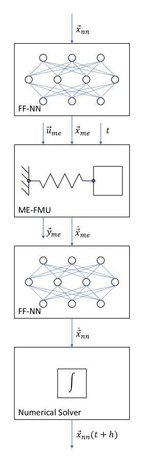
Figure 3: Example for a NeuralFMU (ME).

Different interfaces between the FMU layer and NN are possible. For example, the number of FMU layer inputs could equal the number of FMU layer outputs and be simply the number of model states. In Figure 3, the visualization of the suggested structure is given. The top NN is fed by the current system state $\vec{x}_{nn}$. The NN is able to learn and compensate state-dependent modeling failures like measurement offsets or physical displacements and thresholds. After that, the corrected state vector $\vec{x}_{me}$ is passed to the ME-FMU, and the current state derivative $\dot{\vec{x}}_{me}$ is retrieved. The bottom NN is able to learn additional physical effects, like friction or other forces, from the state derivative vector. Finally the corrected state derivatives $\dot{\vec{x}}_{nn}$ are integrated by the numerical solver, to retrieve the next system state $\vec{x}_{nn}(t+h)$. Note, that the time step size $h$ can be determined by a modern numerical solver like Tsit5 [16], with different advantages like dynamic step size and order adaption. This is a significant advantage in performance and memory cost over the use of recurrent NNs for numerical integration.

Note, that many other configurations for setting up the NeuralFMU are thinkable, e.g.:

• the top NN could additionally generate a FMU input $\vec{u}_{me}$

• the bottom NN could learn from states $\vec{x}_{me}$ or derivatives $\dot{\vec{x}}_{me}$, for a targeted expansion of the model by additional model equations

• the bottom NN could learn from the FMU output $\vec{y}_{me}$ or other model variables, that can be retrieved by fmiGetReal

• there could be a bypass around the FMU between both NNs to forward state-dependent signals from the top NN to the bottom NN

• of course, there is no restriction to fully-connected (dense) layers, other feed-forward layers or even drop-outs are possible

To implement the presented ME-NeuralFMU in Julia, the following code is sufficient:

Listing 3: A NeuralFMU (ME) in Julia.

⬇

net = Chain(

Dense(length(x_nn), ...),

...,

Dense(..., length(x_me)),

x_me -> fmiDoStepME(myFMU, x_me),

Dense(length(dx_me), ...),

...,

Dense(..., length(dx_nn)))

nfmu = ME_NeuralFMU(net, ...)

2.2.2 CS-FMUs

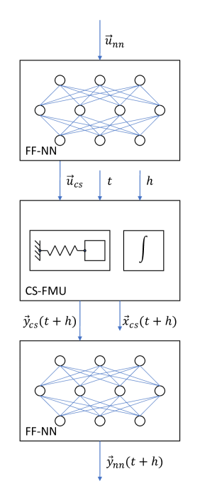
Figure 4: Example for integrating a CS-FMU into a NN.

Beside ME-FMUs, it is also possible to use CS-FMUs as part of NeuralFMUs. For CS-FMUs, a numerical solver like CVODE [7] is already integrated and compiled as part of the FMU itself.

This prevents the manipulation of system dynamics at the most effective point: Between the FMU state derivative output and the numerical integration. However, other tasks like learning an error correction term, are still possible to implement. The presence of a numerical solver leads to a different mathematical description compared to ME-FMUs: The CS-FMU computes the next state $\vec{x}_{cs}(t+h)$ and output $\vec{y}_{cs}(t+h)$ dependent on its internal current state $\vec{x}_{cs}$ (Eq. 3 and 4). Unlike for ME, the state and derivative values of a CS-FMU are not necessarily known (disclosed via FMI).

$$\vec{x}_{cs}(t+h)=\vec{f}_{cs}(\vec{x}_{cs},\vec{u}_{cs},t,h)$$ (3)

$$\vec{y}_{cs}(t+h)=\vec{g}_{cs}(\vec{x}_{cs},\vec{u}_{cs},t,h)$$ (4)

In case of CS-FMUs, the number of layer inputs could be based on the number of FMU-inputs and the number of outputs in analogy. As for ME-NeuralFMUs, this is just one possible setup for a CS-NeuralFMU. Figure 4 shows the topology of the considered NeuralFMU. The top NN retrieves an input signal $\vec{u}_{nn}$, which is corrected into $\vec{u}_{cs}$. Note, that here training of the top NN is only possible if the FMU output is sensitive to the FMU input. This is often not the case for physical simulations. Inside the CS-FMU, the input $\vec{u}_{cs}$ is set, an integrator step with step size $h$ is performed and the FMU output $\vec{y}_{cs}(t+h)$ is forwarded to the bottom NN. Here, a simple error correction into $\vec{y}_{nn}(t+h)$ is performed, meaning the error is determined and compensated without necessarily learning the mathematical representation of the underlying physical effect.

Note that for CS, even if the macro step size $h$ must be determined by the user, it does not need to be constant if the numerical solver inside the FMU supports varying step sizes. If so, the internal solver step size may vary from $h$, in fact $h$ acts as a upper boundary for the internal micro step size. As a result, if the FMU is compiled with a variable-step solver, unnecessarily small values for $h$ will have negative influence on the internal solver performance, but large values will not destabilize the numerical integration.

Other configurations for setting up the hybrid structure are interesting, e.g.:

• the bottom NN could learn from the system state $\vec{x}_{cs}(t+h)$ or state derivative $\dot{\vec{x}}_{cs}(t+h)$

• the step size $h$ could be learned by an additional NN to optimize simulation performance

• there could be a bypass around the FMU between both NNs to forward input-dependent signals from the top NN to the bottom NN

The software implementation of the considered CS-NeuralFMU looks as follows:

Listing 4: A NeuralFMU (CS) in Julia.

⬇

net = Chain(

Dense(length(u_nn), ...),

...,

Dense(..., length(u_cs)),

u_cs -> fmiInputDoStepCSOutput(myFMU, h, u_cs),

Dense(length(y_cs), ...),

...,

Dense(..., length(y_nn)))

nfmu = CS_NeuralFMU(net, ...)

First, the function fmiInputDoStepCSOutput sets all FMU-inputs to the values u, respectively the output of the previous net layer. After that, a fmiDoStep with step size h is performed and finally the FMU output is retrieved and passed to the next layer. Because of the integration over time inside the CS-FMU to retrieve new system states, it is necessary to reset the FMU for every training run, similar to the training of recurrent NNs.

3 Methodical Background

High-performance machine learning frameworks like Flux.jl are using AD for reverse-mode differentiation through the NN topology. Because all mathematical operations inside the NN are known (white-box), this is a very efficient way to derive the gradient and train NNs. On the other hand, the jacobian over a black-box FMU is unknown from the view of an AD framework, because the model structure is (in general) hidden as compiled machine code. This jacobian is part of the loss gradient AD-chain and needs to be determined.

Beside others, the most common and default AD framework in Julia is Zygote.jl. A remarkable feature of Zygote.jl is, that it provides the ability to define custom adjoints, meaning the gradient of a custom function can be defined to be an arbitrary function. This renders the possibility to pass a custom gradient for a FMU-representation to the AD-framework, which will be later used to derive the total loss function gradient during the training process.

3.1 Gradient of the Loss Function

For the efficient training of NNs, the gradient of the loss function according to the net parameters (weights and biases) is needed. In the following, three methods to derive the loss gradient will be discussed: AD, forward sensitivity analysis and backward adjoints. In the following, only ME-NeuralFMUs are considered and the loss function $l(\vec{x}_{nn}(\vec{p}))$ is expected to depend explicitly on the system state $\vec{x}_{nn}$ (the NeuralFMU output) and only implicitly on the net parameters $\vec{p}$.

3.1.1 Automatic Differentiation (AD)

For white-box systems, like native implemented numerical solvers, one possible approach to provide the gradient is AD [12]. In general, the mathematical operations inside a FMU are not known (compiled binary), meaning despite AD being a very common technique, it is only suitable for determining the gradient of the NN, but not the jacobian over a FMU. The unknown jacobian $\vec{J}_{fmu}$ over the FMU layer with layer inputs $\vec{u}$ and outputs $\vec{y}$ is noted as follows:

$$\vec{J}_{fmu}=\frac{\partial\vec{y}}{\partial\vec{u}}$$ (5)

Inserting $\vec{u}=\vec{x}_{me}$ and $\vec{y}=\dot{\vec{x}}_{me}$ results in the jacobian $\vec{J}_{me}$ for the FMU from the example in subsection 2.2.1 (ME), inserting $\vec{u}=\vec{u}_{cs}$ and $\vec{y}=\vec{y}_{cs}(t+h)$ results in the jacobian matrix $\vec{J}_{cs}$ for subsection 2.2.2 (CS):

$$\vec{J}_{me} =\frac{\partial\dot{\vec{x}}}{\partial\vec{x}}$$ (6)

$$\vec{J}_{cs} =\frac{\partial\vec{y}(t+h)}{\partial\vec{u}(t)}\approx\frac{\partial\vec{y}(t)}{\partial\vec{u}(t)}$$ (7)

The simplification in Equation 7 does not lead to problems for small step sizes $h$, because in practice, a small error in the jacobian only negatively affects the optimization performance (convergence speed) and not the convergence itself. However, the quantity of the mentioned error is dependent on the the optimization algorithm and parameterization and $h$ should be selected on the basis of expert knowledge about the model and optimizer or - if not available - as part of hyper parameter tuning.

3.1.2 Forward Sensitivities

To retrieve the partial derivative (sensitivity) of the system state according to a net parameter $p_{i}\in\vec{p}$ and thus in straight forward manner also the gradient of the loss function, another common approach is Forward Sensitivity Analysis. Sensitivities can be estimated by extending the system state by additional sensitivity equations in form of ODEs. Dependent on the number of parameters $|\vec{p}|$, this leads to large ODE systems of size $(1+|\vec{p}|)\cdot|\vec{x}|$ [6, 21] and therefore worsens the overall computation and memory performance. Computations can be reduced, but at a higher memory cost [12, 15]. For a ME-NeuralFMU, the sensitivity equation for a parameter $p_{i}$ can be formulated as in [6, 19]:

$$\frac{d}{dt}\frac{\partial\vec{x}_{nn}}{\partial p_{i}}=\underbrace{\frac{\partial\dot{\vec{x}}_{nn}}{\partial\vec{x}_{nn}}}_{\vec{J}_{nn}}\cdot\frac{\partial\vec{x}_{nn}}{\partial p_{i}}+\frac{\partial\dot{\vec{x}}_{nn}}{\partial p_{i}}$$ (8)

The jacobian of the entire NeuralFMU $\vec{J}_{nn}$ can be described via chain-rule as a product of the three jacobians $\vec{J}_{bottom}$ (over the bottom part of the NN), $\vec{J}_{me}$ (over the ME-FMU) and $\vec{J}_{top}$ (over the top part of the NN):

$$\underbrace{\frac{\partial\dot{\vec{x}}_{nn}}{\partial\vec{x}_{nn}}}_{\vec{J}_{nn}}=\underbrace{\frac{\partial\dot{\vec{x}}_{nn}}{\partial\dot{\vec{x}}_{me}}}_{\vec{J}_{bottom}}\cdot\underbrace{\frac{\partial\dot{\vec{x}}_{me}}{\partial\vec{x}_{me}}}_{\vec{J}_{me}}\cdot\underbrace{\frac{\partial\vec{x}_{me}}{\partial\vec{x}_{nn}}}_{{\vec{J}_{top}}}$$ (9)

Inserting Equation 9 into Equation 8 yields:

$$\frac{d}{dt}\frac{\partial\vec{x}_{nn}}{\partial p_{i}}=\underbrace{\frac{\partial\dot{\vec{x}}_{nn}}{\partial\dot{\vec{x}}_{me}}}_{\vec{J}_{bottom}}\cdot\underbrace{\frac{\partial\dot{\vec{x}}_{me}}{\partial\vec{x}_{me}}}_{\vec{J}_{me}}\cdot\underbrace{\frac{\partial\vec{x}_{me}}{\partial\vec{x}_{nn}}}_{{\vec{J}_{top}}}\cdot\underbrace{\frac{\partial\vec{x}_{nn}}{\partial p_{i}}}_{\vec{g}_{top\_i}}+\underbrace{\frac{\partial\dot{\vec{x}}_{nn}}{\partial p_{i}}}_{\vec{g}_{bottom\_i}}$$ (10)

Retrieving the jacobian $\vec{J}_{me}$ is handled in subsection 3.2, the jacobians $\vec{J}_{bottom}$ and $\vec{J}_{top}$ are determined by AD, because the NN is modeled as white-box and all mathematical operations are known. The remaining gradients, $\vec{g}_{top\_i}$ and $\vec{g}_{bottom\_i}$ can be determined building an AD-chain, dependent on the parameter locations inside the NN (top or bottom part), the jacobian $\vec{J}_{me}$ is needed.

As mentioned, the poor scalability with parameter count makes forward sensitivities unattractive for ML-applications with large parameter spaces, but it remains an interesting option for small NNs. To decide which sensitivity approach to pick for a specific NN size, a useful comparison according to performance of forward and other sensitivity estimation techniques, dependent on the number of involved parameters, can be found in [11].

3.1.3 Backward Adjoints

The performance disadvantage of Forward Sensitivity Analysis motivates the search for a method, that scales better with a high parameter count. Retrieving the directional derivatives over a black-box FMU sounds similar to the reverse-mode differentiation over a black-box numerical solver as in [3]. The name Backward Adjoints results from solving the ODE adjoint problem backwards in time:

$$\vec{a} =\frac{dl(\vec{x}_{nn})}{d\vec{x}_{nn}}$$ (11)

$$\frac{d\vec{a}}{dt} =-\vec{a}^{T}\cdot\underbrace{\frac{\partial\dot{\vec{x}}_{nn}}{\partial\vec{x}_{nn}}}_{\vec{J}_{nn}}$$ (12)

The jacobian $\vec{J}_{nn}$ can be retrieved like in Equation 9. The searched gradient of the loss function is then given as in [6, 22]:

$$\frac{dl(\vec{x}_{nn})}{d\vec{p}}=\vec{a}^{T}(t_{0})\cdot\underbrace{\frac{\partial\vec{x}_{nn}}{\partial\vec{p}}}_{\vec{g}_{top}}(t_{0})+\int_{t_{0}}^{t_{1}}\vec{a}^{T}(t)\underbrace{\frac{\partial\dot{\vec{x}}_{nn}}{\partial\vec{p}}(t)}_{\vec{g}_{bottom}}dt$$ (13)

Here $\vec{g}_{top}$ and $\vec{g}_{bottom}$ can be determined again using AD and $\vec{J}_{me}$. To conclude, the backward adjoint ODE system with dimension $|\vec{x}|$ has to be solved only once independent of the number of parameters and therefore requires less computations for large parameter spaces compared to forward sensitivities. On the other hand, backward adjoints are only suitable, if the loss function gradient is smooth and bounded [6, 22], which limits the possible use for this technique to continuous systems and therefore to almost only research applications.

3.2 Jacobian of the FMU

Independent of the chosen method, the jacobian over the FMU $\vec{J}_{me}$ is needed to keep the NeuralFMU trainable, but is unknown and must be determined. In the following, we suggest two possibilities to retrieve the gradient over a FMU: Finite Differences and the use of the built-in function fmi2GetDirectionalDerivative.

3.2.1 Finite Differences

The jacobian can be derived by selective input modification, sampling of additional trajectory points and estimating the partial derivatives via finite differences. Note, that this approach is an option for ME-FMUs, for CS-FMUs only if the optional functions to store and set previous FMU states, fmi2GetState and fmi2SetState, are available. Otherwise, sampling would require to setup a new simulation for every FMU layer input and every considered time step, if the system state vector is unknown. This would be an unacceptable effort for most industrial applications with large models.

3.2.2 Built-in Directional Derivatives

The preferred approach in this paper is different and benefits from a major advantage of the FMI-standard: Fully implemented FMUs provide the partial derivatives between any variable pair, thus the partial derivative between the systems states and derivatives (ME) or the FMU inputs and its outputs (CS) is known at any simulation time step and does not need to be estimated by additional methods. In FMI 2.0.2, the partial derivatives can be retrieved by calling the optional function fmi2GetDirectionalDerivative [9, 26]. Depending on the underlying implementation of this function, which can vary between exporting tools, this can be a fast and reliable way to gather directional derivatives in fully implemented FMUs.

To conclude, the key step is to forward the directional derivatives over the FMU to the AD-framework Zygote.jl. As mentioned, Zygote.jl provides a feature to define a custom gradient over any function. In this case, the gradients for the functions fmiDoStepME and fmiInputDoStepCSOutput are wrapped to calls to fmi2GetDirectionalDerivative.

Finally, we provide a seamless link to the ML-library Flux.jl, meaning NeuralFMUs can be trained the same way as a convenient NN in Julia:

Listing 5: Training NeuralFMUs in Julia.

⬇

nfmu = NeuralFMU(net, ...)

p_net = Flux.params(nfmu)

Flux.train!(..., p_net, ...)

As a final note, the presented methodical procedure, integrating FMUs into the Julia machine learning environment, can be transferred to other AD-frameworks in other programming languages like Python.

4 Example

When modeling physical systems, it’s often not practical to model solely based on first principle and parameterize every physical aspect. For example, when modeling mechanical, electrical or hydraulic systems, a typical modeling assumption is the negligence of friction or the use of greatly simplified friction models. Even when using friction models, the parameterization of these is a difficult and error prone task. Therefore, we decided to show the benefits of the presented hybrid modeling technique on an easy to understand example from this set of problems.

4.1 Model

Figure 5: The reference system in Modelica.

As in Figure 5, the reference system is modeled as one mass oscillator (horizontal spring-pendulum) with mass $m$, spring constant $c$ and relaxed spring length $s_{rel}$, defined by the differential equation:

$$\ddot{s}=\dot{v}=a=\frac{c\cdot(s_{0}+s_{rel}-s)-f_{fric}(v)}{m}$$ (14)

The parameter $s_{0}$ describes the absolute position of the fixed anchor point, allowing to model a system displacement or a constant position measurement offset. Further, the friction force $f_{fric}$ between the pendulum body and the underlying ground is implemented with the non-linear, discontinuous friction model from MassWithStopAndFriction as part of the Modelica Standard Library (MSL). The friction term for positive $v$ denotes:

$$f_{fric}(v)=f_{coulomb}+f_{prop}\cdot v+f_{stribeck}\cdot e^{-f_{exp}\cdot v}$$ (15)

This friction model consists of parameters for the constant Coulomb-friction $f_{coulomb}$, $f_{prop}$ for the velocity-proportional (viscous) friction and $f_{stribeck}$ for the exponential Stribeck-friction. The FMU (white box) model on the other hand, only covers the modeling of a continuous, frictionless spring pendulum, therefore with $f_{fric}(v)=0$.

The aim here is to learn a generalized representation of the parameterized friction-model in Equation 15 from measurements of the pendulum’s movement over time. Further, a displacement of $s_{0}=0.1\,m$ is added to the FMU model (modeling failure), which should be detected and compensated. Both systems are parameterized as in Table 1.

Table 1: Parameterization of the reference and FMU model.

Parameter	Value	Value	Unit
	ref. model	FMU model
$f_{prop}$	$0.05$	$0.0$	$\nicefrac{{N\cdot s}}{{m}}$
$f_{coulomb}$	$0.25$	$0.0$	$N$
$f_{stribeck}$	$0.5$	$0.0$	$N$
$f_{exp}$	$2.0$	$0.0$	$\nicefrac{{s}}{{m}}$
$mass.m$	$1.0$	$1.0$	$kg$
$spring.c$	$10.0$	$10.0$	$\nicefrac{{N}}{{m}}$
$spring.s_{rel}$	$1.0$	$1.0$	$m$
$fixed.s_{0}$	$0.0$	$0.1$	$m$

4.2 NeuralFMU Setup

We will show, that with a NeuralFMU-structure as in Figure 3, it is possible to learn a simplified friction model as well as the constant system displacement (modeling failure) with a simple fully-connected feed-forward NN as in Table 2. The network topology results from a simple random search hyper parameter optimization for a NeuralFMU model with a maximum of 150 net parameters and 8 layers. All weights are initialized with standard-normal distributed random values and all biases with zeros, except the weights of layer #1 are initialized as identity matrix, to start training with a neutral setup and keep the system closer to the preferred intuitive solution. The loss function is defined as simple mean squared error between equidistant sample points of the NeuralFMU and the reference system.

Table 2: Topology of the example NeuralFMU.

Layer	Inputs	Outputs	Activation
#1 (input)	2	2	identity
#2 (FMU)	2	2	none
#3 (hidden)	2	8	identity
#4 (hidden)	8	8	tanh
#5 (output)	8	2	identity

The corresponding code is available online as part of the library repository.

4.3 Results

4.3.1 Training

After a short training of 2500 runs on 400 data points (each position and velocity), the hybrid model is able to imitate the reference system on training data, as can be seen in Fig. 6 for position and 7 for velocity. The training has not converged yet, further training will lead to a improved fit. For the training case, the system was initialized with $mass.s_{0}=0.5\,m$ (the pendulum equilibrium is at $1.0\,m$) and $mass.v_{0}=0\,\nicefrac{{m}}{{s}}$. Please keep in mind that the NeuralFMU was only trained by data gathered from one single simulation scenario.

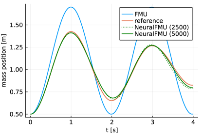
Figure 6: Comparison of the mass position of the FMU, reference system and the NeuralFMU after 2500 and 5000 training steps on training data.

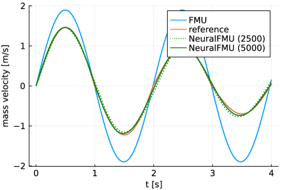
Figure 7: Comparison of the mass velocity of the FMU, reference system and the NeuralFMU after 2500 and 5000 training steps on training data.

4.3.2 Testing

Even if the deviation between NeuralFMU and reference system is larger for testing then for training data, the hybrid model performs well on the test case with a different (untrained) initial system state (Figure 8 and 9). For testing, the system is initialized with $mass.s_{0}=1.0\,m$ and $mass.v_{0}=-1.5\,\nicefrac{{m}}{{s}}$.

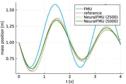
Figure 8: Comparison of the mass position of the FMU, reference system and the NeuralFMU after 2500 and 5000 training steps on testing data.

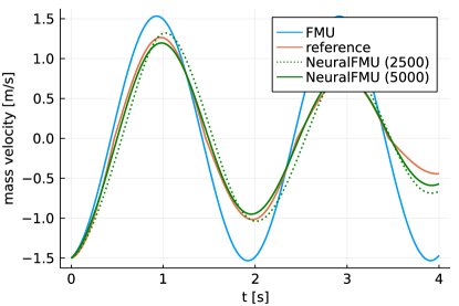
Figure 9: Comparison of the mass velocity of the FMU, reference system and the NeuralFMU after 2500 and 5000 training steps on testing data.

The bottom part of the NN learned the physical effect discontinuous friction in a generalized way, because the net was trained based on the state derivatives instead of the states themselves. A comparison of the friction model of the reference system, the FMU and the learned friction model, extracted from the bottom part NN of the NeuralFMU, is shown in Figure 10. The learned friction model is a simplification of the reference friction model, because of the small net layout and a lack of data at the discontinuity near $v=0$. Finally, also the displacement modeling failure of the white-box model (FMU) was canceled out by the small top NN as can be seen in Figure 11.

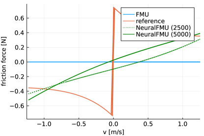
Figure 10: Comparison of the friction models of the FMU, reference system and the NeuralFMU (bottom part NN) after 2500 and 5000 training steps on testing data.

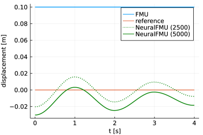
Figure 11: Comparison of the displacements of the FMU, reference system and the NeuralFMU (top part NN) after 2500 and 5000 training steps on testing data.

5 Conclusion

The presented open source library FMI.jl (https://github.com/ThummeTo/FMI.jl) allows the easy and seamless integration of FMI-models into the Julia programming language. FMUs can be loaded, parameterized and simulated using the abilities of the FMI-standard. Optional functions like retrieving the partial derivatives or manipulating the FMU state are available if supported by the FMU. The library release version 0.1.4 is compatible with FMI 2.0.x (the common version at the time of release), supporting upcoming standard updates like FMI 3.0 is planned. The library currently supports ME- as well as CS-FMUs, running on Windows and Linux operation systems. Event-handling to simulate discontinuous ME-FMUs is supported.

The library extension FMIFlux.jl (https://github.com/ThummeTo/FMIFlux.jl) makes FMUs differentiable and opens the possibility to setup and train NeuralFMUs, the structural combination of a FMU, NN and a numerical solver. Proper event-handling during back-propagation whilst training of NeuralFMUs is under development, even if there were no problems during training with the discontinuous model from the paper example. A cumulative publication is planned, focusing on a real industrial use-case instead of a methodical presentation.

Current and future work covers the implementation of a more general custom adjoint, meaning despite Zygote.jl, other AD-frameworks will be supported. Further, we are working on different fall-backs if the optional function fmi2GetDirectionalDerivatives is not available. The finite differences approach for ME-FMUs is already implemented, sampling via fmi2GetState and fmi2SetState for CS-FMUs will be supported soon.

FMUs contain the model as compiled binary, therefore FMU related computations must be performed on the CPU. On the other hand, deploying NNs on optimized hardware like GPUs often results in a better training performance. Currently, the training of the NeuralFMU is completely done on the CPU. A hybrid hardware training loop with the FMU on the CPU and NN on the GPU may lead to performance improvements for wider and deeper NN-topologies.

An extension of the library to the CS-standard SSP [10], including the necessary machine learning back-end, is near completion. This will allow the integration of complete CSs into a NN topology and retrieve a NeuralSSP.

Beside NeuralFMUs, FMIFlux.jl paves the way for other hybrid modeling techniques and new industrial use-cases by making FMUs differentiable in an AD-framework. The authors are excited about any assistance they can get to extend the library repositories by new features and maintain them for the upcoming technology progress. Contributors are welcome.

References

- [1] Jeff Bezanson, Stefan Karpinsky, Viral B. Shah and Alan Edelman “Julia: A Fast Dynamic Language for Technical Computing” In CoRR abs/1209.5145, 2012 arXiv: http://arxiv.org/abs/1209.5145
- [2] Jeff Bezanson, Alan Edelman, Stefan Karpinski and Viral B. Shah “Julia: A Fresh Approach to Numerical Computing” In CoRR abs/1411.1607, 2015 arXiv: http://arxiv.org/abs/1411.1607
- [3] Tian Qi Chen, Yulia Rubanova, Jesse Bettencourt and David Duvenaud “Neural Ordinary Differential Equations” In CoRR abs/1806.07366, 2018 arXiv: http://arxiv.org/abs/1806.07366
- [4] Hilding Elmqvist, Andrea Neumayr and Martin Otter “Modia - Dynamic Modeling and Simulation with Julia” In Juliacon 2018, 2018 URL: https://elib.dlr.de/124133/
- [5] Manuel Haussmann et al. “Learning Partially Known Stochastic Dynamics with Empirical PAC Bayes”, 2021 arXiv:2006.09914 [cs.LG]
- [6] Alan C. Hindmarsh and Radu Serban “User Documentation for CVODES v2.5.0”, 2006 URL: https://www.researchgate.net/profile/Radu-Serban/publication/239581887_User_Documentation_for_CVODES_v210/links/00b7d534f0be2a496f000000/User-Documentation-for-CVODES-v210.pdf
- [7] Alan C. Hindmarsh et al. “User Documentation for CVODE v5.7.0 (sundials v5.7.0)”, 2021 URL: https://computing.llnl.gov/sites/default/files/cv_guide-5.7.0.pdf
- [8] Mike Innes et al. “A Differentiable Programming System to Bridge Machine Learning and Scientific Computing” In CoRR abs/1907.07587, 2019 arXiv: http://arxiv.org/abs/1907.07587
- [9] Modelica Association “Functional Mock-up InterfaceforModel Exchange and Co-Simulation. Document version: 2.0.2”, 2020 URL: https://github.com/modelica/fmi-standard/releases/download/v2.0.2/FMI-Specification-2.0.2.pdf
- [10] Modelica Association “System Structure and Parameterization. Document version: 1.0”, 2019 URL: https://ssp-standard.org/publications/SSP10/SystemStructureAndParameterization10.pdf
- [11] Christopher Rackauckas et al. “A Comparison of Automatic Differentiation and Continuous Sensitivity Analysis for Derivatives of Differential Equation Solutions”, 2018 arXiv:1812.01892 [cs.NA]
- [12] Christopher Rackauckas et al. “DiffEqFlux.jl - A Julia Library for Neural Differential Equations” In CoRR abs/1902.02376, 2019 arXiv: http://arxiv.org/abs/1902.02376
- [13] Christopher Rackauckas et al. “SciML/DifferentialEquations.jl: v6.17.2” Zenodo, 2021 DOI: 10.5281/zenodo.5069045
- [14] Rahul Rai and Chandan K. Sahu “Driven by Data or Derived Through Physics? A Review of Hybrid Physics Guided Machine Learning Techniques With Cyber-Physical System (CPS) Focus” In IEEE Access 8, 2020, pp. 71050–71073 DOI: 10.1109/ACCESS.2020.2987324
- [15] M. Raissi, P. Perdikaris and G.E. Karniadakis “Physics-informed neural networks: A deep learning framework for solving forward and inverse problems involving nonlinear partial differential equations” In Journal of Computational Physics 378, 2019, pp. 686–707 DOI: https://doi.org/10.1016/j.jcp.2018.10.045
- [16] Ch. Tsitouras “Runge–Kutta pairs of order 5(4) satisfying only the first column simplifying assumption” In Computers & Mathematics with Applications 62.2, 2011, pp. 770–775 DOI: https://doi.org/10.1016/j.camwa.2011.06.002
- [17] Jared Willard et al. “Integrating Physics-Based Modeling with Machine Learning: A Survey”, 2020 arXiv:2003.04919 [physics.comp-ph]