QUINT: Node embedding using network hashing

Abstract

Representation learning using network embedding has received tremendous attention due to its efficacy to solve downstream tasks. Popular embedding methods (such as deepwalk, node2vec, LINE) are based on a neural architecture, thus unable to scale on large networks both in terms of time and space usage. Recently, we proposed $\mathrm{BinSketch}$, a sketching technique for compressing binary vectors to binary vectors. In this paper, we show how to extend $\mathrm{BinSketch}$ and use it for network hashing. Our proposal named QUINT is built upon $\mathrm{BinSketch}$, and it embeds nodes of a sparse network onto a low-dimensional space using simple bit-wise operations. QUINT is the first of its kind that provides tremendous gain in terms of speed and space usage without compromising much on the accuracy of the downstream tasks. Extensive experiments are conducted to compare QUINT with seven state-of-the-art network embedding methods for two end tasks – link prediction and node classification. We observe huge performance gain for QUINT in terms of speedup (up to $7000\times$ and space saving (up to $80\times$) due to its bit-wise nature to obtain node embedding. Moreover, QUINT is a consistent top-performer for both the tasks among the baselines across all the datasets. Our empirical observations are backed by rigorous theoretical analysis to justify the effectiveness of QUINT. In particular, we prove that QUINT retains enough structural information which can be used further to approximate many topological properties of networks with high confidence.

1 Introduction

Machine learning tasks that involve networks, such as node classification, clustering, link prediction, find it challenging to use large networks due to the difficulty in succinctly representing their structures. For example, representing the neighborhood information of a node in an $n$-node network would require an $n$-dimensional binary vector or a $k$-dimensional real vector in which $k$ indicates the number of neighbors of any node, and each entry takes $\log n$ bits. This motivated the problem of network embedding, also known as network representation learning, in which each node is assigned a low-dimensional vector such that it maintains the structural or geometric relationship among the nodes.

A number of challenges have been uncovered in the last few decades that have led to a series of studies to propose efficient and effective node embedding methods  [2]. Most embedding techniques “learn” an optimal encoding for specific machine learning tasks. This involves employing an optimization algorithm (say, gradient descent) which usually lacks worst-case guarantees and is also difficult to scale for massive networks. Recently, a few GPU-based approaches were proposed to improve scalability [3]. However, we are interested in CPU-only approaches. Furthermore, the embeddings obtained thus are optimized for specific tasks and may not be effective for others. The final challenge is the space complexity of the embeddings. It is desirable to get a succinct embedding of nodes because of two reasons: (i) It requires less storage; e.g., employing 128 dimensional real-valued vectors costs 1KB of storage per node (on a 64-bit machine) which shoots to 1GB for a million node network. (ii) A succinct embedding leads to faster training and inferencing of machine learning models.

Preserving the semantics of latent representation is another challenge since many proposed techniques are evaluated using statistical methods on standard datasets which may fail to bring out the rich structural invariants that these techniques might be capturing. A few approaches such as deepwalk that captures short random walks [4] and GraRep that captures powers of an adjacency matrix [5], explicitly consider certain structural aspects. However, to the best of our knowledge, how their embeddings fare on other structural properties of a graph is yet to be established.

Of late, randomization has been proved to be highly effective in algorithm design; yet, barring a few approaches based on random walks [4, 6], random projections [7], and random hashing [8], randomized approaches are not extensively studied in the domain of graph embedding. Walking along the relatively less popular path of non-learning based and randomized approaches, we present QUINT, a QUick thIN and biTty mapping of nodes in a sparse network to low-dimensional bit-vectors. The prime takeaway from this work is the affirmation of bit-wise hashing as a sound alternative to learning based methods. It has theoretical bounds on the worst-case situations, delivers comparable (and sometimes better) accuracy with much less space and requires significantly less time compared to the state-of-the-art. This work also suggests that sparse data can be analysed better with sparsity-aware methods; despite many networks being sparse in nature, we are aware of only a handful of approaches specifically for them [9, 10, 11].

Major contributions: Our main contribution is QUINT that takes a large $n$-node network as an input and outputs a $d$-bit binary embedding corresponding to each node. QUINT uses a modified version of $\mathrm{BinSketch}$ [1], a sketching algorithm that we recently proposed for binary data. Here, $d$ denotes the dimension of the embedding, and we give a formula to compute it in terms of the maximum degree of any node of a network (which we will simply denote by ‘degree’ when the context is clear). We make two important modifications to $\mathrm{BinSketch}$, one of them being a larger dimension than what is stipulated by $\mathrm{BinSketch}$; however, it is common for real-world networks to have a low degree compared to the number of nodes, and the best part is that a much smaller $d$ suffices in practice.

Our approach addresses many of the concerns raised above and emerges as a strong contender for node embedding in a resource-constrained scenario — it requires shorter embedding time and generates small-sized embeddings. We emphasise that QUINT is designed to handle networks without attributes and weights.

(i) Speedup in embedding: QUINT takes an adjacency matrix or an edge list of a network as an input and outputs binary embedding of nodes using just one pass over the network while doing bit manipulations. Due to its simplicity, it computes the embeddings in almost real time. For instance, on the BlogCatalog network [12] with $10,312$ nodes and $333,983$ edges, QUINT finishes within $1.6$ secs (for $d=1000$), about $5~{}\mu sec$ per edge; in contrast, node2vec, deepwalk, LINE require 23 mins, 19 mins and 32 mins, respectively, for a single epoch. Similarly, on Flickr [13] network with $80,513$ nodes and $5,899,882$ edge, QUINT finished within $30.63$ secs (for $d=1000$), by taking about $5.2~{}\mu sec$ per edge; on the other hand, node2vec and LINE did not finished in $10$ hours; deepwalk, VERSE and NodeSketch require $2.1$ hr, and $4.8$ hr and $18$ mins, respectively. Also on Youtube network [13] with $1,138,499$ nodes and $2,990,443$ edges, QUINT finished within $35.06$ secs (for $d=1000$), about $11.7~{}\mu sec$ per edge; whereas, node2vec , deepwalk, LINE, VERSE did not finished in $10$ hours and NodeSketch require $15$ mins.

(ii) Less space overhead: Popular embedding methods output real-valued embedding, generally $128$ or $256$ dimensional real-valued vectors, whereas QUINT generates binary embeddings consuming $d$ bits for a $d$-dimensional embedding of a node. In the link prediction task (aka. link discovery) on BlogCatalog, we find that node2vec, NodeSketch, LINE and deepwalk generate $128$-dimensional real-valued vectors that consume $128\times 64=8{,}192$ bits, and these embeddings generate a maximum AUC score of $66$. In contrast, QUINT with $d=1000$ uses only a tenth of that space (1000 bits) to achieve $84.4$ AUC-ROC. Similarly, on Youtube dataset node2vec and NodeSketch for $128$-dimension embedding achieve a maximum AUC score of $65.1$, whereas QUINT with $d=100$ achieve $90$ AUC-ROC value, while using only $1/80$ of space in comparison.

(iii) State-of-the-art accuracy: We compare QUINT with seven recently proposed state-of-the-art embedding methods – node2vec [6], deepwalk [4], LINE [14], Verse [15], NetMF [16], NodeSketch [17], and SGH [18], for link prediction and node classification, and on altogether ten real-world publicly available datasets and several LFR generated synthetic graphs. For our experiments we perform the end tasks considering the embeddings obtained from the competing methods. QUINT remains one of the top performers in terms of accuracy across all the networks and end tasks. We attribute this to $\mathrm{BinSketch}$ that has displayed the ability to generate succinct representations which simultaneously “preserve” multiple similarities [1].

(iv) Supporting theoretical analysis: We also present a rigorous theoretical analysis of the appealing properties that give QUINT an edge over the existing techniques. Embedding obtained from QUINT is essentially a compressed form of the neighborhood information of a node. We show that the embedding, even though compressed, retains information about the network structure such as the degrees, the number of common neighbors, the number of even length paths, etc. More generally, we discuss how any even power of an adjacency matrix can be approximately computed from the embedding with a large confidence and accuracy. Not surprisingly, our embedding allows us to perform link prediction and node classification as good as the others, and sometimes better. We hope that similar performance would be observed for other machine learning tasks (e.g., clustering) that rely only on the structural properties of a network, i.e., without using any metadata.

(v) Sparsity-aware design: Many real-world networks are sparse in nature. However, to the best of our knowledge, most of the embedding approaches do not tend to include optimisations specific to sparse data or provide theoretical guarantees that depend on its sparsity, except a few, e.g., NetSMF [9], STRAP [10], SSNE [11]. QUINT is designed keeping sparse networks in mind. Both the empirical and analytical results explain how QUINT leverages the notion of sparsity of a network, which we quantify by the largest degree among all nodes.

(vi) QUINT vs. uncompressed representation: Since QUINT emdeddings are compressed forms of rows of an adjacency matrix, one may wonder about the payoffs when the uncompressed adjancency lists or the adjacency rows (rows of an adjacency matrix) are instead used as “embeddings”. Adjacency lists of sparse networks are no doubt compact, but are not immediately suitable due to unequal number of neighbors, complete dependence of the embedding on the ordering of nodes, etc. Adjacency rows avoid these problems but are verbose; nevertheless we compare it with QUINT. Quite surprisingly, we find that the classification and prediction performances of QUINT almost match the accuracy using uncompressed adjacency matrix. In fact, on Enron, QUINT achieves $94.75$ AUC score (with $d=4000$) which is close to that with the adjacency matrix ($95.42$ AUC). This shows that our compression retains many of the useful information in its embedding. Notice that the uncompressed embedding, for Enron, is a 36,692-dimensional binary vector, which is almost 9 times the size of that with QUINT with $d=4000$ and can become embarrassingly large for large sparse networks. Compression also improves the training time, e.g., training during link prediction runs out of memory on an uncompressed embedding of Gowalla.

Organisation: We formally state our problem and briefly discuss our earlier work, $\mathrm{BinSketch}$, in this context in Section 2. Related works are discussed in Section 3. Our QUINT embedding method is presented in Section 4 whose theoretical properties and a few related algorithms are discussed in Section 5. In Section 6, we present the results of our empirical evaluation on several real-world datasets against state-of-the-art algorithms. Section 7 concludes the paper with several open questions.

Reproducibility: The datasets that were used are described along with the specific experiments and are publicly available. We have made available the source codes of the techniques that we used, including that of QUINT, on an accessible server [19].

2 Problem statement and background

Let $G=\langle V,E\rangle$ be an unweighted undirected network with $|V|=n$ nodes and $|E|=e$ edges. The network can also be represented by the adjacency matrix $A\in\{0,1\}^{n\times n}$, where $A_{i,j}=1$ implies that there is an edge between node $i$ and node $j$, and is set to $0$ otherwise. We use $A_{i}$ to denote the $i$-th row of $A$, which in turn represents a $|V|$-dimensional binary vector for the node $i$. The sparsity of $A_{i}$ indicates the number of ones in it, representing the degree of that node, and the sparsity of a network, denoted $\psi$, is defined as the largest sparsity of any $A_{i}$.

Node embedding problem: Our aim is to compute a binary embedding of the nodes of a network, essentially an $n\times d$ binary matrix where $d$ (typically $d\ll n$) is the dimension of the embedding, in a manner that preserves local network structures. These structures can be categorized into first, second, third-order proximities and so on, based on their coverage [20].

First-order proximity. The first-order proximity between nodes $i$ and $j$, denoted by $s^{(1)}_{ij}$, captures the presence of an edge between them and is set to $A_{ij}$ for unweighted networks.

Second and higher order proximities. The $k$-th order proximity is defined inductively. Let $s^{(k)}_{i}=[s^{(k)}_{i1},s^{(k)}_{i2},\ldots,s^{(k)}_{in}]$ denote the $k$-th order proximity between node $i$ and the other nodes. Then the $(k+1)$-th order proximity $s^{(k+1)}_{ij}$ between nodes $i$ and $j$ is computed using a suitable “similarity function” between $s^{(k)}_{i}$ and $s^{(k)}_{j}$. A common practice, for example, is to use the inner product for computing similarity.. It should be noted that a high (or low) $k$-th order proximity between two nodes may not automatically establish a high (or low) $(k+1)$-th order proximity between them. Therefore, different embedding techniques target proximities of specific orders [20]. However, we shall explain later how QUINT, in some manner, ensures proximities of multiple orders.

Extension to Binsketch: Recently, we proposed a randomized sketching technique for binary data, named $\mathrm{BinSketch}$ [1]. It compresses high-dimensional sparse binary vectors to extremely compact binary sketches. The sketch of a vector $a\in\{0,1\}^{n}$ is a $d$-dimensional binary vector $\sigma_{a}$ whose $i$-th bit is set to $\displaystyle\bigvee_{j:\pi(j)=i}a_{j}$, where $\pi$ is a random mapping from $\{1,2\ldots,n\}\to\{1,2,\ldots,d\}$. We also proved that these sketches allow efficient estimation of inner product similarity and a few other similarity metrics.

Theorem 1 (Theorem 1,[1]).

The inner product of two binary vectors with sparsity at most $\psi$ can be estimated from their sketches with probability at least ($1-\rho$) and accuracy $O\left(\sqrt{\mathrm{\psi}\ln\tfrac{6}{\rho}}\right)$ if we set the size of the sketches to $d=\mathrm{\psi}\sqrt{\tfrac{\mathrm{\psi}}{2}\ln\tfrac{2}{\rho}}$.

The motivation behind QUINT is the observation that the rows of the adjacency matrix of a network could be embedded in the above manner to low-dimension binary vectors. Further, since the inner product between two adjacency vectors represents the number of common neighbors of the corresponding nodes, it is possible to estimate the number of common neighbors between any two nodes from their embedding vectors. However, it is not clear whether this idea is practical, i.e., whether it would stand up for the common uses of node embedding in different downstream tasks, or even theoretically sound. The contribution of the current paper is an emphatic ‘yes’ to this question, along with the modifications necessary towards this goal.

$\mathrm{BinSketch}$ consists of two major players – an algorithm to generate a sketch and a suite of estimators for several distance measures. The estimator for inner product distance was deemed suitable for node embedding. Our first modification to QUINT is to set a larger embedding dimension in Algorithm 1 for generating a sketch. The second modification is an added check in Algorithm 3 for estimating the number of common neighbors from embeddings, which turns out to be equivalent to the inner product similarity. Though a much smaller dimension appears to be effective in practice, the larger dimension, along with the check, is required to prove the theoretical guarantees on the embeddings offered by QUINT, in particular Theorem 6 and Theorem 10.

In our earlier work on $\mathrm{BinSketch}$, we were solely concerned with sparse binary vectors and estimation of similarity values. Now, with all the modifications stated above, in this work we are interested in the performance of $\mathrm{BinSketch}$ sketches when the binary vectors come from the adjacency vectors of a network. For example, we prove that when our neighborhood estimation algorithm is used, various structural properties of the network can be determined solely from the embeddings. We further report results of network analytics, namely node classification and link prediction, on real networks.

3 Related Work

Popular node embedding methods can be broadly classified into four categories: (1) data independent hashing, (2) learned hashing, (3) factorization based approaches, and (4) deep learning based approaches. Our method falls in the first category which creates small randomized sketches (also known as signatures in literature) without any “learning” from the data. The sketches are designed to allow fast computation of similarity in a suitable space. Lack of any learning step makes these efficient in time; however, the challenge is to ensure that proximities, especially those of the higher orders, can also be computed apart from the similarities. NodeSketch [17] addresses this problem by using “consistent weighted sampling” that can be used to estimate a weighted variant of Jaccard similarity. Our technique, at its core, uses BinSketch  [1] which can be used to estimate Jaccard, Hamming, and a few other similarity measures at the same time.

The learned hashing techniques, on the other hand, create randomized embeddings using a data dependent hash function that is learned from the data. Spectral Hashing [21] uses Laplacian of the corresponding graph, whereas, Scalable Graph Hashing (SGH) [18] avoids computation of the entire node-to-node similarity matrix by doing a feature transformation followed by a sequential learning step.

Factorization based methods represent graph property, e.g. pairwise similarity of nodes, in the form of a matrix and factorize this matrix to obtain node embedding [22, 23]. GraRep [5] factorizes the $k$-th order transition matrix, HOPE [24] and LQANR [25] factorize up to-$k$-order proximity matrix, and NetMF [16] factorizes a matrix obtained using random walks. Recently, INH-MF [26] was proposed to specifically learn a binary embedding using matrix factorization. These techniques come with elegant theoretical promises, but suffers from high complexity in practice due to the optimization steps, e.g., during factorization [27, 28, 29].

Deep learning based approaches for graph embedding broadly fall into two categories. In the first category, a graph is explored using different exploration methods, and then the contexts of the nodes obtained from the random walks are fed into the skip-gram model [30]. Deepwalk preserves higher-order proximity between nodes. It uses depth-first search to generate random walks. node2vec was later proposed based on the same idea, but with the difference that it employs biased random walks that provide a trade-off between breadth-first search and depth-first search exploration strategies. Choosing the right balance between these two enables node2vec to preserve community structure and structural equivalence between nodes. metapath2vec [31] extends a similar approach for Heterogeneous Networks by performing meta-path based random walks to construct the heterogeneous neighborhood of a node and then leverages a heterogeneous skip-gram model to perform node embeddings. A major limitation of such methods is that it only considers a local context within a path. Moreover, it is difficult to determine the optimal sampling strategy. The second category of algorithm does not use any random walk; instead, they model variable-sized subgraph structures in homogeneous graphs. Some examples are GCN [32], GraphSAGE [33], and struc2vec [34]. To summarise, the advantage of deep learning based methods is that they are effective and robust and don’t require feature engineering, but the downside is that they incur a high computational cost.

Slightly less popular, but relevant nonetheless, are matrix-based methods. They are usually difficult to scale without intricate optimizations. For example, RandNE [7] applies SVD to billion-scale networks for which they use Gaussian random projection and the Johnson-Lindenstrauss (JL) Lemma [35]. It should be noted that the JL Lemma is applicable primarily to real vectors and for Euclidean distance; however, we work on binary vectors, and hence, require similarity metrics relevant for binary vectors. To take advantage of bitwise operations that are known for speed and space efficiency, we use our own algorithm, BinSketch [1].

Recently, sketching-based techniques have been explored for generating node embeddings of large networks. Chen et al. [36] proposed an algorithm for computing node embedding of large networks using very sparse random projections [37]. FREDE [38] generates linear space embedding of nodes using deterministic matrix sketching [39], and InstantEmbedding [40] computes node embedding using local PageRank computation. However, all these results lead to real-valued embedding in contrast to the space efficient binary embedding obtained via our approach.

It is common for networks to have attributes associated with their nodes or edges or both. Several solutions have been proposed for embedding such networks. For example, BANE [41] proposes binary embedding of attributed network by joint representation learning of node links and attributes. Along the similar lines, ASNE [42] too generates embedding that tries to retain both structural and attribute proximities, and GNN [29] uses a graph neural network. DNE (Discrete Network Embedding) [43] is a supervised technique which learns binary node representations to speed up node classification by jointly learning the discrete embedding and classifier within a unified framework. While these are all supervised techniques, an unsupervised technique named NetHash was proposed recently that uses a recursive hashing approach for embedding an attributed network [8]. In contrast, QUINT is designed to embed nodes without any attributes.

The “Feature hashing” algorithm due to Weinberger et al. [44] takes high-dimensional real-valued data as input and outputs low-dimensional real-valued vectors (sketch) which closely approximates the original pairwise inner product similarities. If we naively apply Feature hashing on our adjacency matrix, the sketch may not remain binary (node2hash [45] builds upon this idea). BinSketch offers a similar guarantee but generates binary sketches. In this manner, BinSketch can be seen as Feature hashing for binary data that outputs binary vectors and allows approximation of the inner product similarity, the cosine similarity, the Jaccard similarity, and the Hamming distance.

Many of the above techniques generate real-valued embeddings, whereas QUINT generates binary embeddings. There are a few more ways in which our approach follows a quite different trajectory compared to the above approaches. First, we avoid direct operations on the adjacency matrix which can be extremely huge. Secondly, the above approaches try to learn the optimal embedding that minimizes a difference function; the difference function captures the desideratum of accurately obtaining some graph property (e.g., neighborhood of a node) or the effectiveness of the embedding for a certain machine learning task. QUINT deviates from the norm and generates a random embedding upfront in an unsupervised manner. It leaves the heavy duty of using it effectively to algorithms for estimating graph properties, e.g., the degree of a node or the number of length-2 paths between two nodes. We feel that the key factor behind the effectiveness of QUINT is the effective use of the low-sparsity nature of the networks that it was designed for. None of the above techniques are explicitly designed for such networks.

4 QUINT embedding

QUINT uses the $\mathrm{BinSketch}$ sketching algorithm that is appropriately designed for node embedding and modified to obtain theoretical guarantees. We describe it in Algorithm 1. It uses a random mapping, denoted $\pi$, that maps every vertex to a uniformly chosen bin among $d$ bins. To embed a node $v$, it puts the endpoints of all the edges from $v$ into a uniformly and identically chosen bin using $\pi$. The embedding of $v$ is a binary vector indicating which of the $d$ bins are non-empty.

First enhancement to $\mathbf{\mathrm{BinSketch}}$: The first modification that we make is a larger embedding dimension; we set $d=\psi^{2}\sqrt{\frac{\psi}{2}\ln\frac{2}{\rho}}$, where $\psi$ is an upper bound on the degree of any node. This enables us to show that the sketches preserve the higher order proximities with reasonable accuracy (see Theorem 10).

Input: undirected unweighted graph $G=\langle V,E\rangle$       Parameter: probability of error $\rho$

1:Compute $\psi\leftarrow$ upper bound on degree of $G$

2:Embedding dimension $d\leftarrow\psi^{2}\sqrt{\frac{\psi}{2}\ln\frac{2}{\rho}}$ $\triangleright$ Increased from $\mathrm{BinSketch}$

3:$\pi\leftarrow$ a random mapping from $\{1,\ldots,|V|\}$ to $\{1,\ldots,d\}$

4:For all $i=1\ldots|V|$, initialize $\sigma_{i}$ as the vector $\overbrace{00\ldots 0}^{d}$

5:Set $L\leftarrow$ list of edges $E$

6:for all edge $(i,k)\in L$ do

7:     Determine $j=\pi(k)$

8:     Set the $j$-th bit of $\sigma_{i}$ to 1

9:end for

10:return embeddings $\{\sigma_{1},\sigma_{2}\ldots\}$ of all nodes

Algorithm 1 QUINT embedding all nodes of a graph

QUINT falls under the “direct encoding approaches” in a recent categorization of graph representation methods [2]. The “encoding” of a node $i$, represented by its adjacency vector $A_{i}$, is given by the matrix-vector product $P\cdot A_{i}^{T}$ where $P$ is a $d\times n$ matrix. For QUINT, we choose $P$ as a random sparse binary matrix with $n$ ones such that there is exactly one $1$ in any column. For the matrix product, we use a Boolean-logic equivalent of standard matrix product, i.e., the $i$-th entry of the product of a binary matrix $M$, and a binary vector is computed as $\bigvee_{k=1}^{n}(M_{ik}\wedge v_{k})$. An example illustrating this notion is given in Figure 1.

$$\pi:\left[\begin{array}[]{cc}1\to 1&2\to 3\\ 3\to 2&4\to 2\\ 5\to 3&6\to 2\end{array}\right]\qquad\left[\begin{array}[]{c}100000\\ 001101\\ 010010\end{array}\right]\cdot[010110]^{T}=[011]^{T}$$

Figure 1: QUINT embedding of a node with edges to $2,4,5$ is 011. The mapping $\pi$ is shown on the left.

5 Analysing QUINT

In this section, we analyse the theoretical properties of QUINT that make it suitable for embedding graphs while retaining information about its structural properties, and this, we believe, helps in node classification and link prediction. It will be helpful to remember that the embedding of a node $i$ is a $d$-dimensional binary vector which is denoted $\sigma_{i}$ and is defined as:

$\mbox{ $j$-th coordinate of $\sigma_{i}$: }(\sigma_{i})_{j}=\bigvee_{k:\pi(k)=j}A_{ik}$

where $\pi$ denotes a random mapping from $\{1,2,3,\ldots,n\}$ to $\{1,2,3,\ldots,d\}$ and $A$ is the adjacency matrix.

5.1 Time and space complexity

The random mapping can be generated once and stored as a fast-lookup table or can be implemented using an efficient hashing algorithm. Let $S$ denote the space required and $T$ denote the time-complexity to compute $\pi(\cdot)$; for a lookup table stored in RAM, $S=O(n\log d)$ and $T=O(1)$. Apart from the overhead of $\pi$, QUINT only involves bit manipulations which makes it extremely efficient. We assume that $G$ is stored as an adjacency list (which has asymptotically same space complexity as that of an edge-list representation).

Lemma 2.

Algorithm 1 runs in time $\Theta(T\cdot|E|)$, returns an embedding using $d\cdot|V|$ bits and requires an additional space $S$ for the embedding.

We point out that $\pi$ does not need to be stored once a graph is embedded. While the node embeddings can be stored in RAM, another alternative is to not store the embedding, but to store only $\pi$ and generate $\sigma_{i}$ on demand; this approach is also efficient given the lightweight embedding algorithm.

Lemma 3.

The embedding of a single node $i$ uses only $d$ bits and can be computed in time $O(T\cdot n(i))$, where $n(i)$ denotes the degree of $i$, and without any additional space overhead.

Taking $T$ and $d$ to be constant for practical scenarios, both these approaches take constant time per edge of the network and use constant space per node of the network.

5.2 Estimating number of neighbors

The number of neighbors of a node can be easily estimated from its embedding by re-using a result that was proved by us for $\mathrm{BinSketch}$ except that we use a larger $d$ compared to what was used there. Choosing a larger reduced dimension obviously does not adversely affect the accuracy.

Lemma 4 (Lemma 8,[1]).

There is a linear-pass algorithm to estimate the number of neighbors of a node $i$ with at most $4\sqrt{\frac{\psi}{2}\ln\frac{2}{\delta}}$ additive inaccuracy and probability at least $1-\delta$.

5.3 Estimating lower order proximities

We used the “inner product” similarity measure for node classification and link prediction. The first-order proximity between two nodes, say $s_{ij}^{(1)}$, is always the presence of an edge between them, i.e., same as $A_{ij}$. To compute the second-order proximity, observe that $s_{i}^{(1)}=[s_{i1}^{(1)},s_{i2}^{(1)},\ldots s_{in}^{(1)}]$ which is identical to $A_{i}$. Now, $s_{ij}^{(2)}$ is the inner product of $s_{i}^{(1)}$ and $s_{j}^{(1)}$ and this is same as the inner product of $A_{i}$ and $A_{j}$. Further, the latter can be easily shown to be the number of common neighbors of $i$ and $j$ — denoted $n_{i,j}$ (this can also be represented as the $(i,j)$-th entry of $A^{2}$). Note that $n_{i,j}\leq\psi$, degree of the graph.

First we show that QUINT allows us to estimate the first-order proximity for the inner product similarity measure. The first-order proximity between nodes $i$ and $j$ indicates the presence of an edge between them. There was no mention of anything similar in $\mathrm{BinSketch}$ so we show how this can be estimated from their sketches $\sigma(i)$ and $\sigma(j)$ using Algorithm 2.

Input: Nodes $i$ and $j$

Input: Embeddings $\sigma_{i}$ of $i$ and $\sigma_{j}$ of $j$

1:Compute $a=\pi(i)$

2:Compute $b=\pi(j)$ $\triangleright$ $a,b$ could be same or different

3:if $b$-th bit of $\sigma_{i}$ and $a$-th bit of $\sigma_{j}$ are both 1 then

4:     return true

5:else

6:     return false

7:end if

Algorithm 2 Estimate presence of an edge between nodes $i,j$

It is obvious that if there is an edge between nodes $i$ and $j$ then Algorithm 2 is correct, since $i_{j}=j_{i}=1$ and that implies that the $b$-th bit of $\sigma_{i}$ is 1 and so is the $a$-th bit of $\sigma_{j}$. The other case of no edge between $i$ and $j$ is covered by Lemma 5.

Lemma 5.

Algorithm 2 is always correct when there is an edge between $i$ and $j$ and has a probability of error at most $\tfrac{2\psi}{d}\leq\tfrac{2\sqrt{2}}{\psi\sqrt{\psi\ln 2/\rho}}$ when there is no such edge.

Proof.

The proof of the first case is given above. The proof of the second case is obtained by bounding the probability of events $E_{i}=``\pi(k)\not=\pi(j)$ for all neighbor $k$ of $i"$ (there are at most $\psi$ neighbors) and $E_{j}$ is defined similarly for $j$. Note that the probability that the estimator is correct can be expressed as $\Pr[E_{i}\cup E_{j}]$ which is at least $\Pr[E_{i}]+\Pr[E_{j}]-1$. The proof follows from the observation that $\Pr[E_{i}]\geq(1-\tfrac{1}{d})^{\psi}$. ∎

Next we show that QUINT allows us to estimate the second-order proximity using the above similarity measure – the number of common neighbors. We describe this approach in Algorithm 3. Given embeddings $\sigma_{i}$ and $\sigma_{j}$ of nodes $i$ and $j$, respectively, the algorithm first determines the number of ones in those embeddings. Observe that the number of ones in the $i$-th row of $A$ determines the degree of $i$. Conceptually the algorithm will use the number of ones in $\sigma_{i}$ to determine the number of ones in $A_{i}$, albeit with some inaccuracy, and thereby estimate its degree.

Then the algorithm computes the number of common indices where both $\sigma_{i}$ and $\sigma_{j}$ are one, denoted $\hat{n}^{s}_{i,j}$. Once again, the number of common indices where both $A_{i}$ and $A_{j}$ are one is exactly the number of common neighbors they have, and, will be estimated from $\hat{n}^{s}_{i,j}$. It turns out this estimation requires the degrees of $i$ and $j$ whose approximate values we calculated above.

Input: Nodes $i$ and $j$

Input: Embeddings $\sigma_{i}$ of $i$ and $\sigma_{j}$ of $j$

Parameter: Embedding dimension $d$

1:Compute $\hat{n}^{s}_{i}=|\sigma_{i}|$ $\triangleright$ $|v|$: number of ones in vector $v$

2:Compute $\hat{n}^{s}_{j}=|\sigma_{j}|$

3:Compute $\hat{n}^{s}_{i,j}=\langle\sigma_{i},\sigma_{j}\rangle$ $\triangleright$ $\langle u,v\rangle$: inner prod. of $u$ and $v$

4:if $\hat{n}^{s}_{i,j}=0$ then

5:     return $\hat{n}_{i,j}=0$ $\triangleright$ Enhancement from $\mathrm{BinSketch}$

6:end if

7:Set $\hat{n}_{i}=\ln(1-\frac{\hat{n}^{s}_{i}}{d})/\ln(D)$ $\triangleright$ $D$ denotes $1-\frac{1}{d}$

8:Set $\hat{n}_{j}=\ln(1-\frac{\hat{n}^{s}_{j}}{d})/\ln(D)$

9:return estimated number of common neighbors

$$\hat{n}_{i,j}=\hat{n}_{i}+\hat{n}_{j}-\tfrac{1}{\ln D}\ln\left(D^{\hat{n}_{i}}+D^{\hat{n}_{j}}+\frac{\hat{n}^{s}_{i,j}}{d}-1\right)$$

Algorithm 3 EstCN (number of common neighbors $n_{i,j}$)

The next theorem formalizes our claim that the embeddings preserve the second order proximities.

Theorem 6.

Let $\psi$ be an upper bound on the degree of $G$ and $\rho$ be the desired probability of error. If the embedding dimension $d$ is chosen as $\psi^{2}\sqrt{\frac{\psi}{2}\ln\frac{2}{\rho}}$, then EstCN ensures that its output satisfies the following with probability $\geq 1-\rho$.

$$(1)\qquad n_{i,j}-14\sqrt{\frac{\psi}{2}\ln\frac{6}{\rho}}\quad<\hat{n}_{i,j}<\quad n_{i,j}+14\sqrt{\frac{\psi}{2}\ln\frac{6}{\rho}}$$

(2) Furthermore, if $n_{i,j}>0$ then $\hat{n}_{i,j}>0$, and if $n_{i,j}=0$ then $\hat{n}_{i,j}=0$ with probability at least $1-\sqrt{2/(\psi\ln\tfrac{2}{\rho})}$.

Second enhancement to $\mathbf{\mathrm{BinSketch}}$: We quickly discuss the role of the enhancements to $\mathrm{BinSketch}$ in proving this theorem. The first part about the accuracy of ${\tt EstCN}$ in Theorem 6 is known to be a feature of the BinSketch algorithm (refer to Theorem 1), except that the embedding dimension used there was $\psi\sqrt{\frac{\psi}{2}\ln\frac{2}{\rho}}$. Our first modification was a larger value $\psi^{2}\sqrt{\frac{\psi}{2}\ln\frac{2}{\rho}}$. But since the embedding dimension has increased, there are now even lesser chances of collision in the computation of $\pi(\cdot)$ and higher chances that a particular bit of an embedding is set by only one bit of an input vector. Intuitively speaking, this will only result in a better accuracy and lower probability of error during an estimation compared to the that by the BinSketch algorithm.

The second part says that, with high probability, $n_{i,j}=0$ iff $\hat{n}_{i,j}=0$. This is important, since otherwise, the estimated number of common neighbors of $i$ and $j$ could be as large as $14\sqrt{\frac{\psi}{2}\ln\frac{6}{\rho}}$ even when $i$ and $j$ share no common neighbor. The enhancement in Line 5 of Algorithm 3 is crucial to prove the second part.

Both the modifications in Algorithm 1 and Algorithm 3 are neither cosmetic nor heuristic but are necessary to prove Theorem 6, especially that $\hat{n}_{i,j}$ is concentrated around $n_{ij}$ in the second part. This, in turn, enables us to prove Theorem 10 which says that certain higher order proximities are preserved by QUINT.

Proof sketch for the first part.

We present a sketch of the proof here; for the detailed calculations, please refer to our earlier work on $\mathrm{BinSketch}$ [1].

Due to the uniform nature of the random mapping $\pi$ used in Algorithm 1, it is easy to show that $\mathbb{E}[\hat{n}^{s}_{i}]=d\big{(}1-D^{deg(i)}\big{)}$ in which $deg(i)$ denotes the degree of the node $i$; a similar identity also holds for $\hat{n}^{s}_{j}$. These formulæ allow us to express $deg(i)$ in terms of $\mathbb{E}[\hat{n}^{s}_{i}]$.

Next, observe that the $t$-th bit of both $\sigma_{i}$ and $\sigma_{j}$ can be set only in one of two ways.

1. Both $i$ and $j$ have an edge to some node $k$ which is mapped by $\pi$ to $t$.

2. Nodes $i$ and $j$ do not share a common neighbor but the $t$-th bit is set due to some neighbor $a$ of $i$ for which $\pi(a)=t$ and due to some neighbor $b$ of $j$ for which $\pi(b)=t$.

Once again the uniform nature of $\pi$ allows us to express the expected number of bits that are set in both $\sigma_{i}$ and $\sigma_{j}$ by the following formula.

$\displaystyle\mathbb{E}[\hat{n}^{s}_{i,j}]=d\Big{(}1-D^{deg(i)}-D^{deg(j)}+D^{deg(i)+deg(j)+n_{i,j}}\Big{)}$

This expression allows us to express $n_{i,j}$ in terms of $\mathbb{E}[\hat{n}^{s}_{i,j}]$, $deg(i)$ and $deg(j)$, and further, in terms of $\mathbb{E}[\hat{n}^{s}_{i,j}]$, $\mathbb{E}[\hat{n}^{s}_{i}]$ and $\mathbb{E}[\hat{n}^{s}_{j}]$ using the two formulæ given above. This is precisely what Algorithm 3 does. Of course, it does not have the actual expectation values. But fortunately we can show that the observed values of $\hat{n}^{s}_{i,j}$, $\hat{n}^{s}_{i}$ and $\hat{n}^{s}_{j}$ are tightly concentrated around their expectations. In other words, it suffices to use the observed values in place of their expectations in lieu of some inaccuracy in $\hat{n}({i,j})$; the inaccuracy too can be bounded by carefully combining the concentration bounds of $\hat{n}^{s}_{i,j}$, $\hat{n}^{s}_{i}$ and $\hat{n}^{s}_{j}$. ∎

Proof of second part.

For the first claim, we observe that if $n_{i,j}>0$, then there must be some $k$ such that $A_{ik}=A_{jk}=1$. Let $t$ denote $\pi(k)$; then both $(\sigma_{i})_{t}=(\sigma_{j})_{t}$ will be set to 1. Thus, $\hat{n}^{s}_{i,j}=\langle\sigma_{i},\sigma_{j}\rangle>0$. By way of contradiction, assume that $\hat{n}_{i,j}=0$. But then we can derive the following identities based on Algorithm 3.

$$\hat{n}_{i}+\hat{n}_{j} =\tfrac{1}{\ln D}\ln\left(D^{\hat{n}_{i}}+D^{\hat{n}_{j}}+\frac{\hat{n}^{s}_{i,j}}{d}-1\right)$$

$$D^{\hat{n}_{i}}\cdot D^{\hat{n}_{j}} =D^{\hat{n}_{i}}+D^{\hat{n}_{j}}+\frac{\hat{n}^{s}_{i,j}}{d}-1$$

$$\left(1-\frac{\hat{n}^{s}_{i}}{d}\right)\left(1-\frac{\hat{n}^{s}_{j}}{d}\right) =\left(1-\frac{\hat{n}^{s}_{i}}{d}\right)+\left(1-\frac{\hat{n}^{s}_{j}}{d}\right)+\frac{\hat{n}^{s}_{i,j}}{d}-1$$

$$\frac{\hat{n}^{s}_{i}\cdot\hat{n}^{s}_{j}}{d^{2}} =\frac{\hat{n}^{s}_{i,j}}{d}\implies\frac{|\sigma_{i}|}{d}\cdot\frac{|\sigma_{j}|}{d}=\frac{\langle\sigma_{i},\sigma_{j}\rangle}{d}$$

The last identity may not always hold. For example, consider a scenario in which $\sigma_{i}\sim\sigma_{j}$ with the number of ones in each much less than $d$; in this case $|\sigma_{i}|\approx|\sigma_{j}|\approx\langle\sigma_{i},\sigma_{j}\rangle$ and $|\sigma_{i}|\ll d$, thus contradicting the identity. This proves that $\hat{n}_{i,j}>0$.

For proving the second claim, take any $i$ and $j$ such that $n_{i,j}=0$, i.e., there is no $k$ such that both $A_{i,k}=A_{j,k}=1$. For the sake of contradiction, assume that $\hat{n}_{i,j}>0$, i.e., there is some $x$ such that $(\sigma_{i})_{x}=(\sigma_{j})_{x}=1$; this means that there must be some $k_{1}$ and $k_{2}$ such that $A_{i,k_{1}}=A_{j,k_{2}}=1$ and $\pi(k_{1})=\pi(k_{2})=x$. The probability for the latter event, denoted $E$, is same as the probability that in a group of $|A_{i}|$ men and $|A_{j}|$ women, there exists at least one pair with a common birthday, which can be shown to be

$$1-\sum_{k=1}^{|A_{i}|}{D\choose k}k!\,S_{|A_{i}|,k}(d-k)^{|A_{j}|}/d^{|A_{i}|+|A_{j}|}$$

in which $S_{\cdot,\cdot}$ denotes Stirling’s number of the second kind [46]. Getting a closed form of this is difficult; therefore, we show a different technique of bounding the probability of $E$.

Let $E_{x}$ be the event that $(\sigma_{i})_{x}=(\sigma_{j})_{x}=1$. It can be shown that $\mathbb{E}(E_{x})=\left(1-D^{|A_{i}|}\right)\cdot\left(1-D^{|A_{j}|}\right)$ [1, Lemma 5]. Since $|A_{i}|$ and $|A_{j}|$ are both at most $\psi$, and $D<1$,

$$\mathbb{E}(E_{x})\leq(1-D^{\psi})^{2}=\left(1-\left(1-\frac{1}{d}\right)^{\psi}\right)^{2}\leq\left(\frac{\psi}{d}\right)^{2}$$

which implies that $\mathbb{E}[\sum_{x}E_{x}]=d\left(\frac{\psi}{d}\right)^{2}=\frac{\sqrt{2}}{\sqrt{\psi\ln\frac{2}{\rho}}}\ll 1$

Let $E_{all}$ denote $\sum_{x}E_{x}$; $E_{all}$ is a random variable that denotes the number of positions $x$ such that $(\sigma_{i})_{x}=(\sigma_{j})_{x}=1$ and whose expectation we computed above. Since $E$ is equivalent to “$E_{all}\geq 1$”, we apply Markov’s inequality to bound it.∎

For the rest of this section, we will use the fact that EstCN estimates non-zero $n_{i,j}$ values with a small additive error and accurately identifies $n_{i,j}=0$ values (both of these happen with non-negligible probability which we would not explicitly state to simplify calculations).

The above theorem allows us to accurately quantify the loss function (aka. objective function) that is used by most node embedding algorithms to learn the embedding [2]. Using the mean-squared-error (MSE) to compute the loss function, we can represent it as

$$\mathcal{L}=\frac{1}{T}\sum_{(i,j)\in T\subseteq V\times V}|n_{i,j}-{\tt EstCN}(i,j)|^{2}.$$

Here $T$ represents a “training set of edges” that is traditionally used to learn an embedding. Our proposed technique does not involve any learning; nevertheless, for the sake of comparison we present an explicit upper bound on $\mathcal{L}$ — it follows directly from Theorem 6.

Lemma 7.

Using QUINT for embedding and EstCN for estimating node similarity, $\mathcal{L}$ is upper bounded by $196\frac{\psi}{2}\ln\frac{6}{\rho}$.

5.4 Estimating higher-order proximities

Many node embedding algorithms operate on the paths in a graph, often up to a certain length. For example, both the random-walk based approaches, deepwalk and node2vec, consider two nodes to be similar if their presence in short random walks on the graph are highly correlated. Here we show that QUINT also “preserves” path information in a certain manner. The key observation here is that the square of the adjacency matrix precisely contains the $n_{ij}$ values.

Observation 8.

For any $i,j$, $A^{2}_{i,j}=n_{i,j}$.

This holds due to the following calculation.

$$\sum\limits_{k=1}^{n}A_{ik}A_{kj}=|\{k\in V~{}:~{}(i,k)\in E,~{}(k,j)\in E\}|.$$

This observation along with Theorem 6 implies that EstCN can approximately compute $A^{2}$.

Lemma 9.

${\tt EstCN}(\sigma_{i},\sigma_{j})$ approximately computes $A^{2}_{i,j}$ with a small additive error. If $A^{2}_{i,j}=0$ ${\tt EstCN}(\sigma_{i},\sigma_{j})$ outputs 0.

Next we show how to translate the above lemma to higher even powers of $A$. We first show the result for the $4$-th power, $A^{4}$, each of whose entry, say $A^{4}_{i,j}$, denotes the number of paths between $i$ and $j$ using 4 nodes (and 3 edges).

We use $\epsilon_{2}$ to denote the small additive error mentioned in Lemma 9. To maintain consistency of notations, we will use $\hat{n}2_{i,j}$ to denote $\hat{n}_{i,j}$; by construction, $\hat{n}2$ is symmetric.

Theorem 10.

Let $\hat{n}4_{i,j}$ denote the expression $\sum_{k=1}^{n}\hat{n}2_{i,k}\cdot\hat{n}2_{k,j}$ for all $i,j=1\ldots n$. Then $\hat{n}4_{i,j}$ approximately computes $A^{4}_{i,j}$ with a small additive error. If $A^{4}_{i,j}=0$ then $\hat{n}4_{i,j}$ outputs 0.

Proof.

Recall that $A^{4}_{i,j}=\sum_{k=0}^{n}A^{2}_{i,k}A^{2}_{k,j}=\sum_{k=0}^{n}A^{2}_{i,k}A^{2}_{j,k}$, and further more, each term in the summation is non-negative. Therefore, $A^{4}_{i,j}=0$ implies that $A^{2}_{i,k}=0$ and $A^{2}_{j,k}=0$ for every $k=1\ldots n$. We know from Lemma 9 that, in this case, $\hat{n}2_{i,k}=0$ and $\hat{n}2_{j,k}=0$ for all $k$. Clearly, $\hat{n}4^{i,j}=0$ too — this proves the second part of the theorem.

For the first part, take any $x,y$ such that $A^{4}_{x,y}>0$. That is, $\sum_{k=1}^{n}A^{2}_{x,k}A^{2}_{y,k}>0$. From Lemma 9 we know that ${|\hat{n}2_{x,y}-A^{2}_{x,y}|\leq\epsilon_{2}}$; using $z$ to denote the left-hand side, we can write $\hat{n}2_{x,y}=A^{2}_{x,y}+z$ where $-\epsilon_{2}\leq z\leq\epsilon_{2}$.

We now state a technical result about $A$.

Claim 11.

$\sum_{u=1}^{n}A^{2}_{x,u}\leq\psi^{2}$.

Proof.

$\psi$ being an upper bound on the degree of any node, the total number of length-2 paths from $x$ is at most $\psi^{2}$. $A^{2}_{x,u}$ is the total number of length-2 paths from $x$ to $u$ and $\sum_{u}A^{2}_{x,u}$ is the total number of length-2 paths from $x$ to any node, which is, therefore, upper bounded by $\psi^{2}$. ∎

The next observation is applicable to sparse graphs in general but immensely beneficial to graphs where $\psi^{2}\ll n$.

Observation 12.

Since the entries of $A^{2}_{x,u}$ are non-negative, Claim 11 implies that at most $\psi^{2}$ entries are non-zero in the $x$-th row of $A^{2}$, i.e, among $A^{2}_{x}=\{A^{2}_{x,u}~{}:~{}u\in\{1,2,\ldots,n\}\}$. That is, at least $n-\psi^{2}$ entries of $A^{2}_{x}$ are zero.

This observation, along with Lemma 9, implies that for any $x$, at most $\psi^{2}$ values in the set $\{\hat{n}2_{x,u}~{}:~{}u\in\{1,2,\ldots n\}\}$ are non-zero. We use $(\sum_{u=1}^{n})^{\leq\psi^{2}}$ to denote the fact that in a summation with $n$ summands, at most $\psi^{2}$ terms are non-zero. Getting back to proving the theorem,

$$\hat{n}4_{x,y}= \sum_{u=1}^{n}\hat{n}2_{x,u}\cdot\hat{n}2_{y,u}$$

$$= (\sum_{u=1}^{n})^{\leq\psi^{2}}(A^{2}_{x,u}+z)\cdot(A^{2}_{y,u}+z)$$

$$= \sum_{u=1}^{n}A^{2}_{x,u}\cdot A^{2}_{y,u}+z\cdot\sum_{u=1}^{n}A^{2}_{x,u}$$

$$+z\cdot\sum_{u=1}^{n}A^{2}_{y,u}+(\sum_{u=1}^{n})^{\leq\psi^{2}}z^{2}$$

$$= A^{4}_{x,y}+2z\psi^{2}+z^{2}\psi^{2}$$ (Using Claim 11)

Thus we get,

$$\big{|}\hat{n}4_{x,y}-A^{4}_{x,y}\big{|}=\big{|}2z+z^{2}\big{|}~{}\psi^{2}=\left\{\begin{array}[]{ll}3|z|\psi^{2}&\mbox{ if $|z|<2$}\\ 2z^{2}\psi^{2}&\mbox{ if $|z|\geq 2$}\end{array}\right.$$

Since $|z|\leq\epsilon_{2}$ and the additive error $\epsilon_{2}$ for $\hat{n}^{2}_{x,y}$ is $\tilde{O}(\sqrt{\psi})$ from Theorem 6 (here $\tilde{O}()$ hides $\log(1/\rho)$ factors), so both $|z|,z^{2}$ is $\tilde{O}(\psi)$. Therefore, the additive error for $\hat{n}4_{x,y}$ is $\tilde{O}(\psi^{3})$. ∎

Theorem 10 can be generalized to show that entries of $A^{2^{t}}$, for $t\geq 1$, can be approximated with additive error $\tilde{O}(poly(\psi))$. Since any even power of $A$ can be written as a product of $A$ raised to a power of 2, we have established that our QUINT embedding effectively preserves all even powers of the adjacency matrix $A$, and therefore, can approximate information about paths of even lengths in $G$.

6 Empirical Evaluation

We first describe our experimental setup. Then we report how our proposed solution performs on two end tasks – node classical and link prediction, with specific emphasis on speed and quality.

Hardware description: We performed most of our experiments on a laptop with the following configuration: Intel(R) Core(TM) i7-4710MQ CPU @ 2.50GHz x 8, 7.5 GB RAM, Ubuntu 18.04 64-bits OS. The experiments on the Gowalla [47], Youtube [13], and Flickr [13] datasets were performed on a server with the following configuration: Intel(R) Xeon(R) CPU E5-2650 v3 @ 2.30GHz, 94 GB RAM, Ubuntu 64-bits OS.

Baseline methods: We evaluated our approach against seven state-of-the-art node embedding methods – node2vec [6], deepwalk [4], LINE [14], VERSE [15], NetMF [16], NodeSketch [17], and SGH [18]; SGH generates binary embedding like QUINT. Since QUINT generates the embedding of a node by compressing its adjacency vector, we also performed experiments using the uncompressed adjacency matrix where the $i$-th row of the matrix is used as the embedding of the $i$-th node; we refer to this method as “Uncompressed”.

TABLE I: Datasets used for link prediction.

Dataset	Nodes	Edges	Max. degree
Gowalla	196,591	950,327	14,730
Enron Emails Network	36,692	183,831	1,383
Facebook	4,039	88,234	1,045
BlogCatalog	10,312	333,983	3,992
Flickr	80,513	5,899,882	5,706
Youtube	1,138,499	2,990,443	28,754

TABLE II: Comparison of space required for storing embeddings

Method	dimension	$\#$ of binary bits
node2vec, deepwalk, LINE, VERSE, NetMF, NodeSketch	128	$128\times 64=8,192$ (64-bits for floating pt.)
QUINT, SGH	$d$	$d$
Uncompressed	$|V|$	$|V|$ (no. of nodes)

TABLE III: Comparison on AUC-ROC and compression time of QUINT and other baselines (using 128 dimensions) for the link prediction experiments. For the datasets on which QUINT outperformed the baselines, we have reported the performance of QUINT on the smallest dimension at which it outperformed the latter; for the other datasets we have reported the best performance of QUINT (see Table XI in Supplementary for the results for all the dimensions). We stopped baselines that took 10 hours or more and indicate them by DNS; OOM indicates baselines that ran out of memory. Smaller datasets were embedded to a maximum of 4000 dimensions. The best AUC-ROC among the baselines and for QUINT are bolded.

Method	Gowalla			Flickr			Youtube
	Dim.	AUC-ROC	Time(s)	Dim.	AUC-ROC	Time(s)	Dim.	AUC-ROC	Time(s)
node2vec	128	75.48	7827	128	76.4	8706.8	128	65.1	30899.28
deepwalk	128	74.79	7075	128	67.7	4978.64	128	$-$	DNS
LINE	128	$-$	DNS	128	$-$	DNS	128	$-$	DNS
VERSE	128	87.35	4902.8	128	91.6	9469.08	128	$-$	DNS
NetMF	128	$-$	OOM	128	$-$	OOM	128	$-$	OOM
NodeSketch	128	50.02	328.30	128	50.03	770.65	128	50.04	538.81
SGH	128	$-$	OOM	128	$-$	OOM	128	$-$	OOM
QUINT	1000	87.71	7.15	100	86.7	7.41	100	90	8.86
Uncompressed	$-$	OOM	$-$	$-$	OOM	$-$	$-$	OOM	$-$

Method	Enron			BlogCatalog			Facebook
	Dim.	AUC-ROC	Time(s)	Dim.	AUC-ROC	Time(s)	Dim.	AUC-ROC	Time(s)
node2vec	128	67.13	560	128	63.12	979.02	128	93.64	63.98
deepwalk	128	66.7	515.36	128	61.00	774.31	128	93.10	54.39
LINE	128	75.87	4216	128	66.08	2379	128	83.41	250.25
VERSE	128	97.20	1058.42	128	74.24	351.38	128	94.32	88.34
NetMF	128	83.98	62.29	128	71.68	7.7	128	94.86	2.02
NodeSketch	128	49.99	44.07	128	50.00	75.53	128	50.00	10.69
SGH	128	71.49	31.28	128	70.05	7.53	128	92.20	5.3
	1600	68.00	106.01	2400	75.36	84.74	1800	88.89	50.32
QUINT	4000	94.75	9.05	100	81.60	0.88	4500	95.30	0.53
Uncompressed	$-$	95.42	$-$	$-$	86.46	$-$	$-$	95.44	$-$

For node2vec, we used the implementation provided by its authors. We did a grid search over its parameters $p$ and $q\in[0.25,0.5,1,2,4]$, which is equivalent to running $25$ different experiments. Here we only report the result for the optimum choice of $p$ and $q$. deepwalk is a special case of node2vec when $p=q=1$ [6], so the earlier node2vec implementation was used here with the specified parameters. For LINE, we used a standard implementation available online and performed experiments considering both first and second order proximity — and reported the best result. VERSE [15] uses the idea of personalised PageRank to compute the embedding of nodes. NetMF [16] unifies the idea of sampling based algorithms such as node2vec, deepwalk, LINE in the matrix factorisation framework to generate embeddings. NodeSketch [17] is built on top of an efficient sketching technique, and it outputs embeddings which preserve higher-order proximity via a recursive approach. SGH [18] learns the binary embedding of nodes by minimizing the difference between the similarity of a pair of nodes and the Hamming similarity of the corresponding binary hash codes.

The embeddings obtained from QUINT, SGH, and full adjacency matrix representation are binary, whereas the other algorithms output real-valued vectors. A real-valued vector that is represented using 64-bit floating point numbers (a common configuration) takes $64\times$ more space as compared to a binary vector of the same dimension. We summarise this in Table II. For all the algorithms which give real-valued embeddings, we report the results of embedding in $128$ dimensions in this section. The results for embedding in 256 dimensions are similar and are given in Tables IX, X, and XII in Supplementary.

6.1 Comparing performance on link prediction

In the link prediction problem, we are given a network with a certain fraction of missing edges, and the task is to predict these missing edges. It can be recast as a classification problem where the goal is to train a classifier that, given a pair of nodes, outputs if there is an edge between them.

For the purpose of classification, we generated a labeled dataset of edges by splitting a dataset into training and testing partition in $70-30$ ratio. To generate the positive training and testing samples, we randomly sampled $30\%$ of edges and removed them. During the removal of edges, we made sure that the residual graph obtained after edge removal remains connected. If the sampled edges do not ensure this, we chose a different edge. We then generated “missing edges” equal in number to those in the original dataset — these are “edges” that are absent in the graph. We split the generated missing edges into training and testing partition in $70-30$ ratio to form negative training and testing samples, respectively. We computed inner product for all the edges and labeled them $0$ or $1$ depending on whether it is a missing edge or an actual edge. Then we combined the positive and negative test samples to form the test data.

We learned embedding of the graph using all the candidate algorithms on our training samples. To measure the performance of the classifier on the embeddings, we calculated the inner product similarity among the embeddings of a pair of nodes from the test data; for QUINT, we used the EstCN algorithm to estimate similarities. We trained a logistic regression on the final training data considering AUC-ROC as our evaluation metric.

Datasets: Gowalla [47] is a location-based social networking website where users share their locations by checking-in. The dataset consists of a total of $6,442,890$ check-ins of these users over the period of Feb. 2009 - Oct. 2010. Enron Emails Network [47] covers all the email communication within a dataset of around half million emails. Nodes of the network are email addresses and if an address $i$ sent at least one email to address $j$, the graph contains an undirected edge from $i$ to $j$.  BlogCatalog [12] is the social blog directory which manages the bloggers and their blogs. The dataset contains the friendship network crawled and group memberships. Here, nodes represent users, and edges represent a friendship relation between any two users. In the Facebook [47] network, nodes represent users, and edges represent friendship relations between users.

We used two social network datasets – Flickr and YouTube [13]. Flickr dataset is of photo-sharing social network, where labels represent the self-identified interests of particular users and edges correspond to the messages between two users. YouTube dataset is a video-based social network of user interactions where labels indicate interest in a particular video genre. We use these datasets, and BlogCatalog, for both node classification and link prediction experiments. Statistics of these datasets are summarised in Table I.

Empirical results and insights: Table III summarizes the comparative analysis (Table XI in Supplementary has the complete details). We observed significant speedup for QUINT in compression time, along with better accuracy as compared to the other candidate algorithms. For instance, on the Gowalla dataset (using 1000 dimensions for QUINT), we obtained $46\times$ to $10^{4}\times$ speedup on the compression times w.r.t. the other candidate algorithms. Our embedding also saves on space as well (see Table II).

It is evident that AUC-ROC for QUINT is comparable with the best among the baselines (a tie on Gowalla and Facebook and a close second on Flickr and Enron), and sometimes even better (on Youtube, BlogCatalog), but always using a fraction of their times. VERSE turns out to be worthy alternative for all the datasets but Youtube, but it is a lot slower because it learns an embedding by running a single-layer neural network.

An attractive property of $\mathrm{BinSketch}$ is the ability to recover different types of similarities from its sketches, e.g., inner product, cosine similarity, etc. QUINT inherits them too. We conducted link prediction experiments using three other similarity measures — cosine similarity, $\ell_{1}$ and $\ell_{2}$ norm, and observed a similar trend that QUINT offered significant speedup in the compression time while offering comparable AUC-ROC scores with respect to the baselines (see Table VII in Supplementary). This shows that QUINT embeddings may be applicable for multiple similarity measures.

TABLE IV: Datasets used for node classification. The first three datasets are also used for link prediction.

Dataset	# Nodes	# Edges	# Classes	Max. degree
Flickr	80,513	5,899,882	195	5706
Youtube	1,138,499	2,990,443	35	28,754
BlogCatalog	10,312	333,983	39	3,992
IMDB	19,773	3,86,124	1000	540
Pubmed	19,717	44,338	3	171
Citeseer	3,327	4,732	6	26
Cora	2,708	5,429	7	5

TABLE V: Comparison on Micro $F_{1}$, Macro $F_{1}$ and compressions time of QUINT and other baselines (using 128 dimensions) for the task of node classification. For the datasets on which QUINT outperformed the baselines, we have reported the performance of QUINT on the smallest dimension at which it outperformed the latter; for the other datasets we have reported the best performance of QUINT (see Tables VIII and X in Supplementary for the results for all the dimensions). We stopped baselines that took 10 hours or more and indicate them by DNS; OOM indicates baselines that ran out of memory. The best Macro $F_{1}$ scores among the baselines and for QUINT are bolded.

Method		Flickr			Youtube				IMDB
	Dim.	Micro$F_{1}$	Macro$F_{1}$	Comp.	Dim.	Micro$F_{1}$	Macro$F_{1}$	Comp.	Dim.	Micro$F_{1}$	Macro$F_{1}$	Comp.
		Score	Score	time(s)		Score	Score	time(s)		Score	Score	time(s)
node2vec	128	$-$	$-$	DNS	128	$-$	$-$	DNS	128	51.91	51.6	117
deepwalk	128	41.2	29.61	2.1 hr	128	$-$	$-$	DNS	128	50.68	50.34	118
LINE	128	$-$	$-$	DNS	128	$-$	$-$	DNS	128	41.25	40.56	1850
VERSE	128	41.52	31.41	4.8 hr	128	$-$	$-$	DNS	128	63.09	63.08	1194.10
NetMF	128	$-$	$-$	OOM	128	$-$	$-$	OOM	128	60.30	51.88	21.72
NodeSketch	128	22.37	7.1	1057.30	128	37.55	26.98	902.68	128	55.69	46.64	6.98
SGH	128	$-$	$-$	OOM	128	$-$	$-$	OOM	128	70.83	70.75	110.78
	3000	$-$	$-$	OOM	128	$-$	$-$	OOM	3000	74.51	74.49	174.12
QUINT	20000	37.04	29.99	59.89	3000	37.80	33.40	67.53	2000	83.88	83.85	3.89
Uncompressed	$-$	OOM	OOM	$-$	$-$	OOM	OOM	$-$	$-$	94.90	95.91	$-$

Method	Citeseer				Cora				Pubmed				BlogCatalog
	Dim.	Micro$F_{1}$	Macro$F_{1}$	Comp.	Dim.	Micro$F_{1}$	Macro$F_{1}$	Comp.	Dim.	Micro$F_{1}$	Macro$F_{1}$	Comp.	Dim.	Mic.$F_{1}$	Mac.$F_{1}$	Comp.
		Score	Score	time(s)		Score	Score	time(s)		Score	Score	time(s)		Score	Score	time(s)
node2vec	128	29.77	21.90	1.75	128	52.76	41.31	1.72	128	43.2	31.34	5.88	128	38.90	23.19	1359.25
deepwalk	128	25.05	17.06	1.77	128	44.15	28.64	1.49	128	42.46	35.15	5.78	128	41.82	28.24	1167.95
LINE	128	36.72	32.72	17.14	128	56.33	53.51	15.72	128	58.19	53.81	840.25	128	20.17	10.15	1898.23
VERSE	128	32.93	29.18	71.83	128	52.27	46.70	53.2	128	42.29	31.93	806.98	128	41.78	29.04	847.4
NetMF	128	49.69	44.06	1.39	128	57.68	52.65	1.43	128	66.00	53.85	19.88	128	43.45	29.05	72.39
NodeSketch	128	25.65	21.26	0.41	128	39.72	30.39	0.5	128	43.79	33.77	4.31	128	19.76	8.66	66.36
SGH	128	37.77	33.37	2.79	128	56.45	52.96	2.54	128	51.10	44.80	67.67	128	13.20	4.05	18.25
	2000	38.77	35.60	53.68	2000	57.93	56.07	36.33	2000	54.83	49.68	122.77	3000	9.02	4.74	120.27
QUINT	3500	50.68	45.99	0.286	1000	61.62	60.43	0.055	2000	68.27	65.50	2.50	10000	37.70	25.51	2.35
Uncompressed	$-$	51.40	47.06	$-$	$-$	65.75	66.66	$-$	$-$	76.52	74.98	$-$	$-$	38.23	25.65	$-$

6.2 Comparing performance on node classification

For node classification, every node is assigned one or more labels from a given set. The dataset is randomly divided into 70% and 30% for training and testing, respectively. We repeated the experiment 10 times for each network and report the average accuracy. We used logistic regression as classifier. Unlike the experiments on link prediction where a subgraph with 70% edges is embedded to generate training data, embedding of the entire network is first computed for the node classification experiments; this shows up in the form of larger compression times.

Datasets: Some of the datasets used for link prediction are not labelled and hence, they are not suitable for node classification. So we used three additional citation datasets — Cora, Citeseer and Pubmed [48] for the experiments. Here, citation relationships are viewed as directed edges. Attributes associated with nodes are extracted from the title and the abstract of the each article and are presented as sparse bag-of-word vectors, after removing the stop words and low-frequency words. Each article in these datasets has only one label representing the class it belongs to. We also considered IMDB-BINARY [49, 50], which is a movie collaboration dataset where actor/actress and genre information of different movies on IMDB are collected. Nodes represent actors/actresses, and an edge between them signifies a joint appearance in some movie. Collaboration graphs is generated on the “action” and the “romance” genres and ego-networks are derived for each actor/actress. A movie can belong to both genres at the same time, therefore movies from the romance genre are discarded if they are already included in the action genre. Each ego-network is labeled with the genre graph it belongs to. The task is then simply to identify which genre an ego-network graph belongs to. All the datasets are summarised in Table IV.

Empirical results and insights: Table V summarizes the performance of the competing algorithms (see Table VIII for complete details) which show a similar trend as in the link prediction experiments. Many baselines failed to generate an embedding of Flickr and/or Youtube datasets within 10 hours, or ran out of memory; however, QUINT did not have any such difficulty and was able to comfortably finish all embedding tasks within a few minutes, mostly taking a few seconds.

Compared with the baselines that could finish embedding within 10 hours, QUINT achieved a higher Macro F1 on Youtube, IMDB, Citeseer, Cora, Pubmed and was a close second on Flickr. It fell behind by 10-15% on BlogCatalog which could be due its network characteristics; even Uncompressed, that which QUINT tries to improve upon, was unable to obtain a high score on that network. The general conclusion that we can draw is that QUINT offers significant speed-up during node embedding while offering comparable accuracy for node classification when compared with the state-of-the-art techniques.

6.3 Comparing Uncompressed with QUINT.

We also want to draw attention towards the Uncompressed embedding. However naïve it may sound, empirically it appears that the neighborhood of a node, when represented as an array, is a reasonably good embedding for the purposes of link prediction and node classification (see the last rows of Tables III and V). The challenge is that training on such embeddings of a large network (e.g., Flickr with 80K nodes) is almost impossible on off-the-shelf hardware. Even for smaller networks, the training time is significantly higher compared to the QUINT embeddings. We list out the speed-up in training time of QUINT over Uncompressed in Table VI. QUINT embeddings are a compressed version of Uncompressed embeddings, and we can safely conclude that it is able to strike a good balance between speed and accuracy.

TABLE VI: Comparison on speedup in training time on embeddings generated using QUINT vs. Uncompressed. We choose the embedding dimension of QUNIT on which it outperforms (or reaches sufficiently close to) the best baselines.

Dataset	Gowalla	Flickr	Youtube	Enron	BlogCatalog		Facebook	IMDB	Pubmed	Citeseer	Cora
					Link pred.	node class.
Dim. of QUINT	1000	100	100	2000	100	5000	1000	1000	1000	2000	1000
Speedup (training time)	OOM	OOM	OOM	96.16$\times$	86.4$\times$	24.8$\times$	31.25$\times$	77.65$\times$	10.48$\times$	2.80$\times$	4.92$\times$

6.4 Performance on training size

We varied the training size in our experiments to show how the competing algorithms react to this variation. For this we split the datasets into various ratios of training and test partitions, starting at $10\%$ training and $90\%$ test partitions, and moving to $90\%$ training and $10\%$ test partitions at intervals of $10\%$. We ran node classification and link prediction on these partitions and observed the Micro F1 and AUC-ROC scores, respectively. We compared the performance of QUINT w.r.t. other candidate algorithms for these experiments, and report the results for two datasets in Figure 2. The results for the other datasets were similar.

We noticed that for node classification on the Cora dataset the Micro $F_{1}$ score always remains higher as compared to the other candidate algorithms (we obtained a similar result on Macro $F_{1}$ score as well). For link prediction on the Enron dataset, we noticed that the AUC-ROC score is comparable to that of VERSE and significantly better than the other baselines. This essentially confirms that even on small training data, QUINT maintains its competitive advantage w.r.t. other baselines.

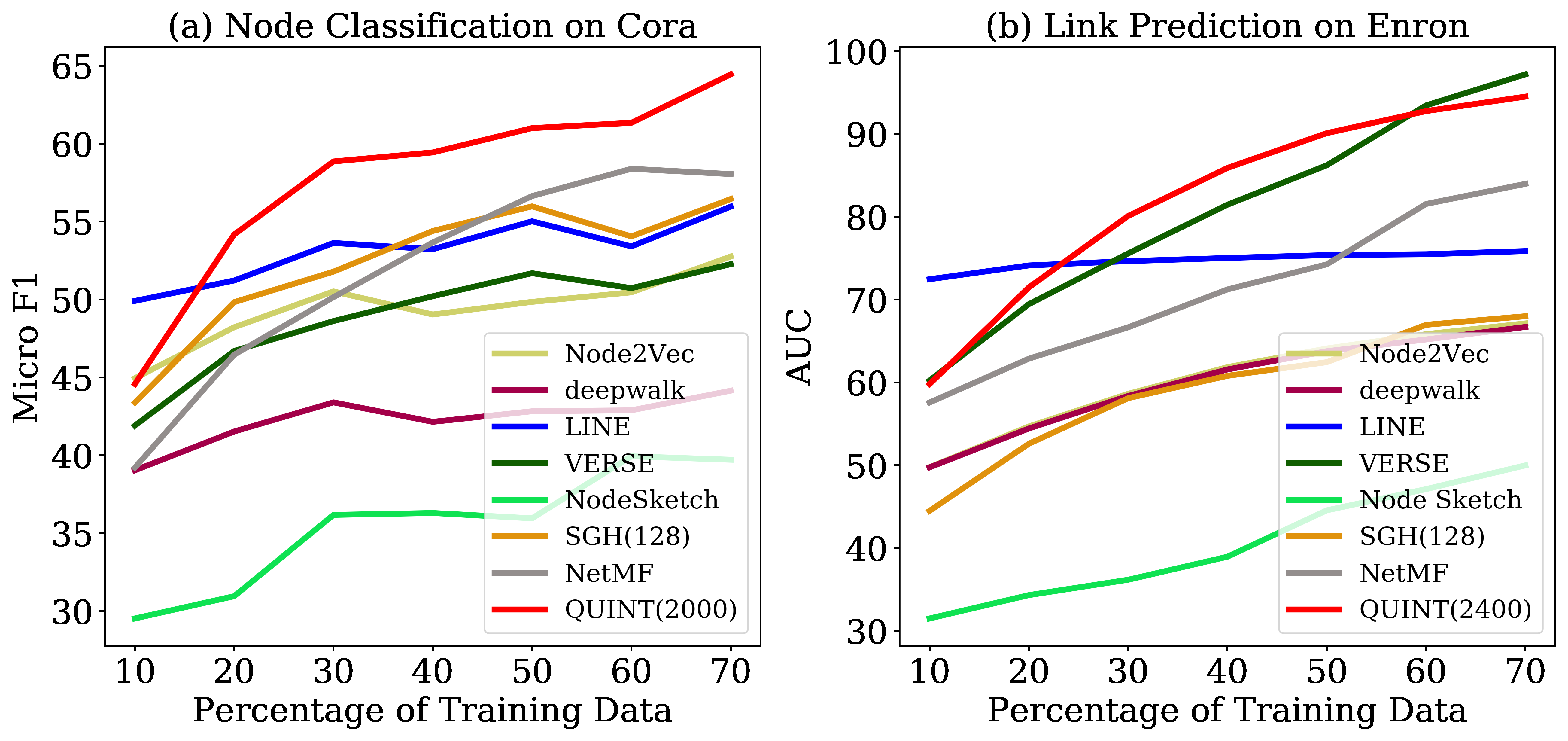
Figure 2: Performance of the baselines on various training/test splits. Figure (a) summarises the Micro $F_{1}$ scores vs $\%$ of training data  of various  baselines on node classification for the Cora dataset. Figure (b) summarises the AUC-ROC scores vs $\%$ of training data of various baselines on link prediction for the Enron dataset. 

6.5 Scalability experiments

Due to the bitwise operations and simplicity of Algorithm 1, the time taken by QUINT increases very slowly in the embedding dimension. This was evident in our experiments on the real-life datasets (see Section A and Tables VIII and XI in Supplementary).

To evaluate the effect of the size of a network, we experimented with link prediction on synthetically generated LFR graphs [51] of varied nodes and edges generated using Python NetworkX with parameters $\mu=0.1,\tau_{1}=2,\tau_{2}=1.1$. The first set of experiments were on graphs with 10K to 100K nodes and second were on graphs with 50K nodes and 1000K to 10,000K edges; the AUC-ROC scores and compression times of QUINT and the baseline algorithms are plotted in Figures 3 and 4, respectively. We observed that in both the experiments, QUINT, when embedded on $1000~{}-~{}4000$ dimensions, is consistently producing a high AUC-ROC along with node2vec, deepwalk, VERSE and netmf. Few of the baselines, including netmf, did not run for the graph with 1000K nodes, and QUINT exhibited one to four orders of speedup for the rest.

Figure 3: Comparing link prediction performance of QUINT and the baseline algorithms on LFR graphs by varying the number of nodes in a network. The left plot compares the AUC-ROC scores and the right plot compares the corresponding compression times. SGH gives OOM error for $70K$ and $100K$ nodes, and NetMF gives OOM error for $100K$ nodes.

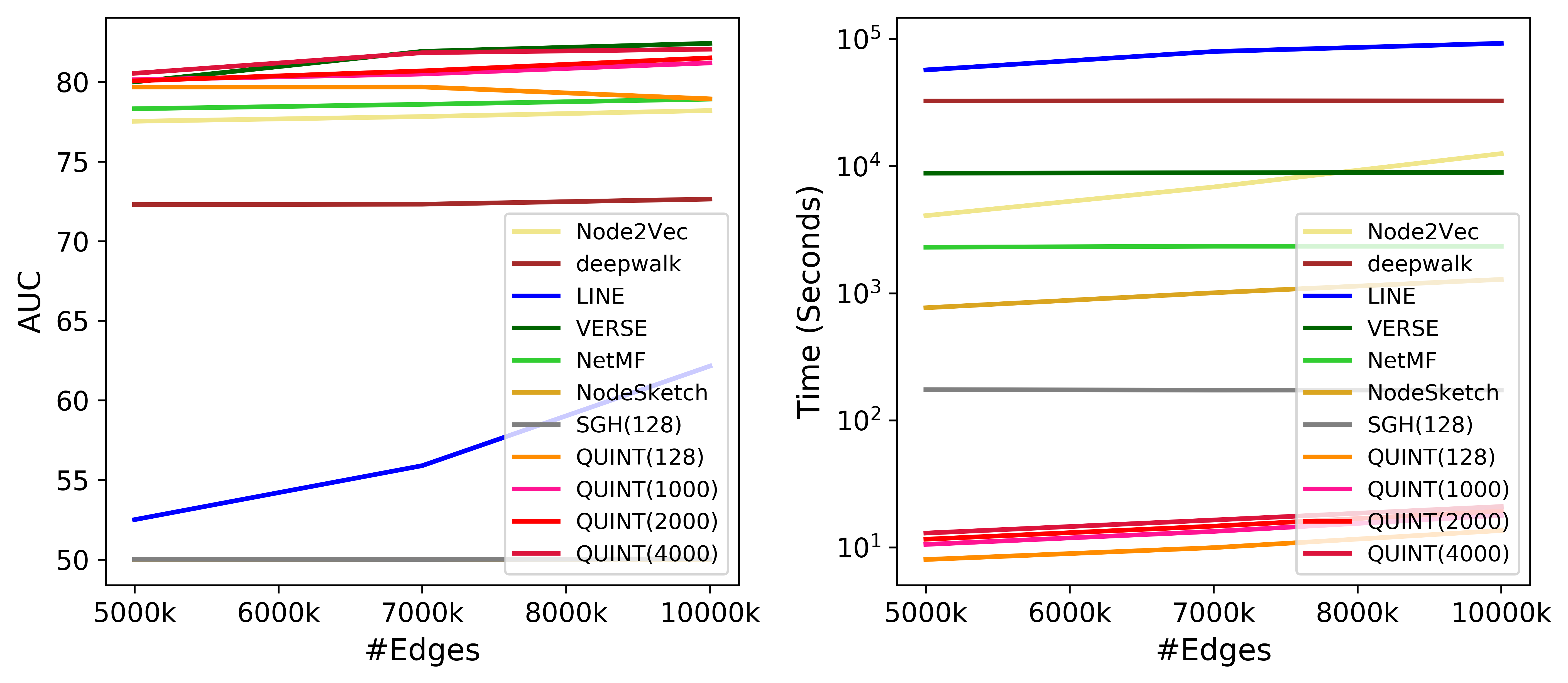
Figure 4: Comparing link prediction performance of QUINT and the baseline algorithms on LFR graphs by varying the number of edges in a network with 50K nodes. The left plot compares the AUC-ROC scores and the right plot compares the corresponding compression times.

7 Conclusion and open questions

In this work, we proposed QUINT which takes a large scale graph as input and outputs succinct low-dimensional binary embedding for each node. The major advantage of QUINT is that it is extremely fast – it computes the embedding of a large graph in almost real time. QUINT does not have a strong hardware requirement and consumes less space for computing and storing the embedding of a graph. In fact, most of our experiments were conducted on an off-the-shelf laptop. We evaluated the performance of QUINT on the task of node classification and link prediction and noticed that  QUINT offers massive speed up in compression time while offering comparable performance with respect to the state-of-the-art algorithms. Moreover, our embedding is binary which makes it space efficient as compared to the real-valued embeddings generated by the most of the baselines.

QUINT has a few added advantages that could be explored further. First is applicability in the sense that the same embedding can be used for both link prediction and node classification, and we conjecture that the same would be applicable to other machine learning tasks based on structural properties of networks, like node clustering. The second advantage comes from the bitwise nature of QUINT. It maybe possible to use QUINT in a distributed setting where embeddings of different groups of nodes are generated on different machines and then combined. Observe that the combination of multiple QUINT embeddings is simply their bitwise-OR.

The final advantage is in regards to evolving networks. We do not consider them in this work but we do make the observation that QUINT embeddings are easy to update. This is since an addition of a new edge, say between nodes $i$ and $j$, essentially leads to setting one bit each in the embeddings of $i$ and $j$ and this can be done independently. To the best of our understanding, most learning-based algorithms would require solving an optimization problem afresh which may mean running their entire algorithm once again.

Our work leaves open the possibility of several future directions. First, we wonder if our results can be extended to efficiently embed hypergraphs? Hypergraphs are a common choice to model non-binary relationships but are difficult to analyse due to high complexity of even simple tasks. A few solutions have been proposed for clustering, classification, and other data analytic tasks based on spectral techniques [52] and random walk [53]. A binary embedding technique ala. QUINT would make hypergraphs considerably easy to handle.

On the theoretical side it would be worth exploring what specific structural features of networks can be efficiently estimated from their embeddings. For example, global clustering coefficient of nodes could be one such candidate since it is basically the ratio of the number of triangle and an expression involving degree of each node. The number of triangles involving a pair of nodes, say $u$ and $v$, can be written as $n_{u,v}\cdot E_{u,v}$, in which $n_{u,v}$ denotes the number of other nodes that are connected to both $u$ and $v$, and $E_{u,v}$ is an indicator variable denoting the presence of an edge between $u$ and $v$. We have shown earlier how to estimate $n_{u,v}$ (Theorem 6) and $E_{u,v}$ (Lemma 5). Thus we conjecture that it should be possible to estimate global clustering coefficient with reasonable accuracy.

There is obviously the question of what other practical applications QUINT, rather $\mathrm{BinSketch}$, is capable of? One way to extend QUINT would be by making it use the attributes associated with nodes and edges of a graph. Randomization may once again prove beneficial but we do not have a solution in sight. Given the affinity of QUINT towards sparse graphs, we wonder whether QUINT can be successful for graphs that are sparse for individual features but dense otherwise. We hope that our simple yet powerful technique can be easily adapted to bring forth efficient solutions to challenging graph embedding problems.

Debajyoti Bera received his B.Tech. in Computer Science and Engineering in 2002 at Indian Institute of Technology (IIT), Kanpur, India and his Ph.D. degree in Computer Science from Boston University, USA in 2010. Since 2010 he is an assistant professor at Indraprastha Institute of Information Technology, (IIIT-Delhi), India. His research interests include quantum computing, randomized algorithms, and engineering algorithms for networks, data mining, and information security.

Rameshwar Pratap has earned Ph.D in Theoretical Computer Science in 2014 from Chennai Mathematical Institute (CMI). Earlier, he completed Masters in Computer Application (MCA) from Jawaharlal Nehru University and BSc in Mathematics, Physics, and Computer Science from University of Allahabad. Post Ph.D he has worked TCS Innovation Labs (New Delhi, India), and Wipro AI-Research (Bangalore, India). Since 2019 he is working as an assistant professor at School of Computing and Electrical Engineering (SCEE), IIT Mandi. His research interests include algorithms for dimensionality reduction, robust sampling, and algorithmic fairness.

Bhisham Dev Verma is pursuing Ph.D from IIT Mandi. He has done his Masters in Applied Mathematics from IIT Mandi and BSc in Mathematics, Physics, and Chemistry from Himachal Pradesh University. His research interest includes data mining, algorithms for dimension reduction, optimization and machine learning.

Biswadeep Sen is currently working as a research associate (remotely) at department of Computer Science, National University of Singapore (NUS), since July, 2020. He completed M.Sc. in Computer Science and B.Sc. in Mathematics and Computer Science from Chennai Mathematical Institute (CMI) in 2018 and 2016, respectively. His research interests include Machine Learning, Artificial Intelligence, Computer Vision and Computational Sustainability.

Tanmoy Chakraborty is an Assistant Professor and a Ramanujan Fellow at the Dept. of CSE, IIIT-Delhi, India, where he leads Laboratory for Computational Social Systems (LCS2). His primary research interests include Social Network Analysis, Data Mining, and Natural Language Processing. He has received several awards including Faculty Awards from Google, IBM and Accenture; Early Career Research Award, DAAD Faculty Fellowship.

QUINT: Node embedding using network hashing (Appendix)

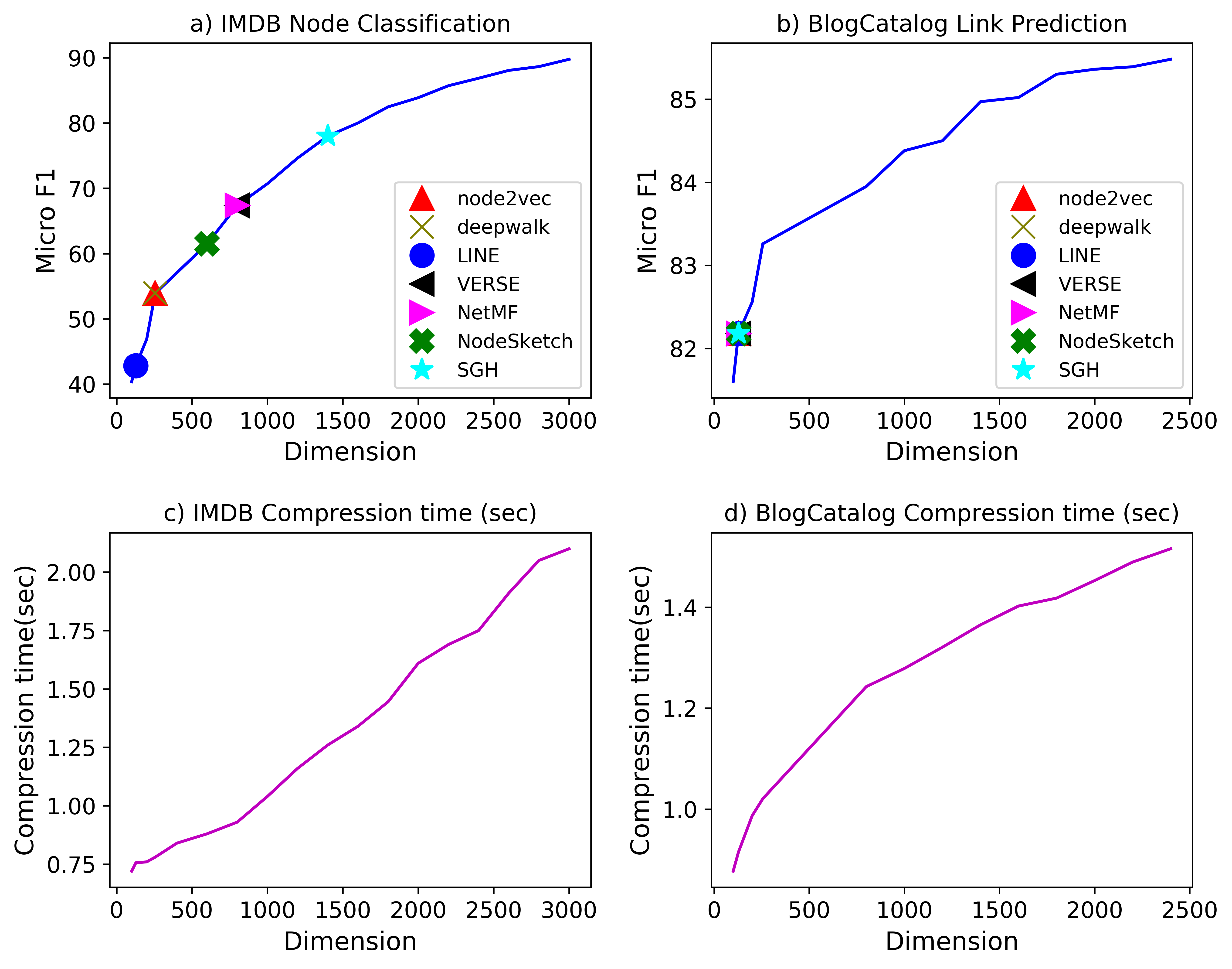
Figure 5: Figure (a) shows the dimensions at which QUINT’s node classification performance on the IMDB dataset matches that of various baselines, and Figure (c) shows the time QUINT takes to do so. Figures (b) and (d) show the same for link prediction on the BlogCatalog dataset.

Appendix A Effect of embedding dimension

The optimum embedding dimension for QUINT on any dataset is theoretically upper-bounded by an expression on its sparsity (the largest degree of a node). However, it is evident from Tables III and V that much lower dimensions works in practice. Further, we observed that embedding on a higher dimension is not much slower and requires at most a few additional seconds (see Tables XI and VIII in Supplementary for the compression times on all dimensions).

To illustrate this observation further, we plot the performance and compression times of QUINT against embedding dimension for the IMDB dataset and the BlogCatalog dataset, for node classification and link prediction, respectively. Figures 5(a) and 5(c) show the embedding dimensions of QUINT at which it matches the performance of the other baselines. Figures 5(b) and 5(d) show the times taken by QUINT when it matches the baselines. These figures show that QUINT is able to match the performance of the baselines for node classification on IMDB and link prediction on BlogCatalog, and that too in only a few seconds (similar figures can be inferred from Tables III and V for the other datasets and baselines that QUINT matches).

TABLE VII: Result of link prediction on the BlogCatalog dataset where instead of inner product, we use few other similarity measures.

Method	BlogCatalog (cosine similarity)			BlogCatalog ($\ell_{1}$ norm)			BlogCatalog ($\ell_{2}$ norm)
	Dim.	AUC-ROC	Time (s)	Dim.	AUC-ROC	Time (s)	Dim.	AUC-ROC	Time (s)
node2vec	128	65.93	979.02	128	75.09	979.02	128	75.36	979.02
deepwalk	128	61.6	774.31	128	82.66	774.31	128	82.83	774.31
LINE	128	65.07	2379	128	65.15	2379	128	36.79	2379
VERSE	128	79.3	351.38	128	61.32	351.38	128	62.47	351.38
NetMF	128	62.18	7.7	128	79.54	7.7	128	79.84	7.7
NodeSketch	128	61.12	75.53	128	50.00	75.53	128	50.00	75.53
SGH	128	49.95	7.53	128	49.99	7.53	128	49.95	7.53
QUINT	100	84.88	0.88	100	65.65	0.88	100	65.74	0.88
	128	84.77	0.92	128	72.18	0.92	128	72.82	0.92
	200	84.10	0.99	200	80.98	0.99	200	81.16	0.99
	256	83.87	1.02	256	83.8	1.02	256	84.24	1.02
	1000	79.69	1.28	1000	85.48	1.28	1000	86.4	1.28
	2000	77.3	1.45	2000	85.22	1.45	2000	86.36	1.45
	3000	76.18	1.62	3000	85.07	1.62	3000	86.31	1.62
	4000	75.29	1.77	4000	85.02	1.77	4000	86.29	1.77
Uncompressed	$-$	74.63	$-$	$-$	84.60	$-$	$-$	86.16	$-$

TABLE VIII: Comparison on Micro $F_{1}$, Macro $F_{1}$ and compressions time of QUINT and other baselines (using 128 dimensions) for the task of node classification. We stopped baselines that took 10 hours or more and indicate them by DNS; OOM indicates baselines that ran out of memory. Smaller datasets were embedded to a maximum of 3000 dimensions. The best Macro $F_{1}$ scores among the baselines and for QUINT are bolded.

Method		Flickr			Youtube				IMDB
	Dim.	Micro$F_{1}$	Macro$F_{1}$	Comp.		Micro$F_{1}$	Macro$F_{1}$	Comp.	Dim.	Micro$F_{1}$	Macro$F_{1}$	Comp.
		Score	Score	time(s)		Score	Score	time(s)		Score	Score	time(s)
node2vec	128	$-$	$-$	DNS		$-$	$-$	DNS	128	51.91	51.6	117
deepwalk	128	41.2	29.61	2.1 hr		$-$	$-$	DNS	128	50.68	50.34	118
LINE	128	$-$	$-$	DNS		$-$	$-$	DNS	128	41.25	40.56	1850
VERSE	128	41.52	31.41	4.8 hr		$-$	$-$	DNS	128	63.09	63.08	1194.10
NetMF	128	$-$	$-$	OOM		$-$	$-$	OOM	128	60.30	51.88	21.72
NodeSketch	128	22.37	7.1	1057.30		37.55	26.98	902.68	128	55.69	46.64	6.98
SGH	128	$-$	$-$	OOM		$-$	$-$	OOM	128	70.83	70.75	110.78
	3000	$-$	$-$	OOM		$-$	$-$	OOM	3000	74.51	74.49	174.12
QUINT	100	19.59	5.4	20.86		28.66	16.65	17.90	100	40.37	39.78	0.72
	128	21.08	7.3	23.11		30.38	20.10	20.46	128	42.82	41.35	0.756
	200	23.58	10.68	23.88		32.31	22.76	20.80	200	46.91	46.48	0.76
	256	25.41	12.46	25.80		32.67	24.10	26.74	256	53.89	52.45	0.78
	1000	28.04	18.61	30.63		35.22	31.63	35.06	1000	70.7	70.58	1.04
	2000	30.12	21.76	33.65		36.56	31.69	51.57	2000	83.88	83.85	1.61
	3000	31.52	23.58	36.07		37.80	33.40	67.53	3000	89.76	89.81	2.1
	4000	32.35	25.05	38.47		38.93	35.12	83.37
	6000	33.98	26.54	41.85		39.61	35.89	111.52
	8000	34.66	27.31	44.86		40.94	37.06	140.08
	10000	35.08	28.10	46.87		41.20	37.46	167.94
	16000	36.86	29.75	55.23		42.41	38.01	250.03
	20000	37.04	29.99	59.89		43.26	38.68	325.48
Uncompressed	$-$	OOM	OOM	$-$		OOM	OOM	$-$	$-$	94.90	95.91	$-$

Method	Citeseer				Cora				Pubmed
	Dim.	Micro$F_{1}$	Macro$F_{1}$	Comp.		Micro$F_{1}$	Macro$F_{1}$	Comp.		Micro$F_{1}$	Macro$F_{1}$	Comp.
		Score	Score	time(s)		Score	Score	time(s)		Score	time(s)
node2vec	128	29.77	21.90	1.75		52.76	41.31	1.72		43.2	31.34	5.88
deepwalk	128	25.05	17.06	1.77		44.15	28.64	1.49		42.46	35.15	5.78
LINE	128	36.72	32.72	17.14		56.33	53.51	15.72		58.19	53.81	840.25
VERSE	128	32.93	29.18	71.83		52.27	46.70	53.2		42.29	31.93	806.98
NetMF	128	49.69	44.06	1.39		57.68	52.65	1.43		66.00	53.85	19.88
NodeSketch	128	25.65	21.26	0.41		39.72	30.39	0.5		43.79	33.77	4.31
SGH	128	37.77	33.37	2.79		56.45	52.96	2.54		51.10	44.80	67.67
	2000	38.77	35.60	53.68		57.93	56.07	36.33		54.83	49.68	122.77
QUINT	100	34.3	28.42	0.024		44.65	38.58	0.02		47.71	39.27	0.2
	128	34.95	28.75	0.029		46.37	41.71	0.021		48.63	42.55	0.21
	200	36.51	28.98	0.035		51.78	47.87	0.024		50.62	43.12	0.23
	256	38.55	29.80	0.038		54.12	50.55	0.027		52.96	47.58	0.25
	1000	44.16	38.79	0.076		61.62	60.43	0.055		63.28	59.63	1.23
	2000	48.28	43.16	0.112		63.59	61.64	0.094		68.27	65.59	2.50
	3000	49.15	43.98	0.214		64.945	64.32	0.124		69.25	66.32	3.75
	3500	50.68	45.99	0.286
Uncompressed	$-$	51.40	47.06	$-$		65.75	66.66	$-$		76.52	74.98	$-$

TABLE IX: Comparison on Micro $F_{1}$, Macro $F_{1}$ and compressions time of QUINT and other baselines (using 256 dimensions) for the task of node classification. We stopped baselines that took 10 hours or more and indicate them by DNS; OOM indicates baselines that ran out of memory. Smaller datasets were embedded to a maximum of 3000 dimensions. The best Macro $F_{1}$ scores among the baselines and for QUINT are bolded.

Method	Flickr				Youtube
	Dim.	Micro$F_{1}$	Macro$F_{1}$	Comp.	Dim.	Micro$F_{1}$	Macro$F_{1}$	Comp.
		Score	Score	time(s)		Score	Score	time(s)
node2vec	256	$-$	$-$	DNS	256	$-$	$-$	DNS
deepwalk	256	41.26	30.06	16286	256	$-$	$-$	DNS
LINE	256	$-$	$-$	DNS	256	$-$	$-$	DNS
VERSE	256	41.29	30.95	23498.55	256	$-$	$-$	DNS
NetMF	256	$-$	$-$	OOM	256	$-$	$-$	OOM
NodeSketch	256	21.56	0.688	2530.36	256	36.29	26.11	2233.81
SGH	256	$-$	$-$	OOM	256	$-$	$-$	OOM
QUINT	100	19.59	0.54	20.86	100	28.66	16.65	17.90
	128	21.08	0.73	23.11	128	30.38	20.10	20.46
	200	23.58	10.68	23.88	200	32.31	22.76	20.80
	256	25.41	12.46	25.80	256	32.67	24.10	26.74
	1000	28.04	18.61	30.63	1000	35.22	31.63	35.06
	2000	30.12	21.76	33.65	2000	36.56	31.69	51.57
	3000	31.52	23.58	36.07	3000	37.80	33.40	67.53
	4000	32.35	25.05	38.47	4000	38.93	35.12	83.37
	6000	33.98	26.54	41.85	6000	39.61	35.89	111.52
	8000	34.66	27.31	44.86	8000	40.94	37.06	140.08
	10000	35.08	28.10	46.87	10000	41.20	37.46	167.94
	16000	36.86	29.75	55.23	16000	42.41	38.01	250.03
	20000	37.04	29.99	59.89	20000	43.26	38.68	325.48
Uncompressed	$-$	OOM	OOM	$-$	$-$	OOM	OOM	$-$

Method	IMDB				Pubmed
	Dim.	Micro$F_{1}$	Macro$F_{1}$	Comp.	Dim.	Micro$F_{1}$	Macro$F_{1}$	Comp.
		Score	Score	time(s)		Score	Score	time(s)
node2vec	256	49.16	50.81	138.79	256	41.39	29.99	6.77
deepwalk	256	47.33	46.12	256.61	256	42.51	35.23	12.29
LINE	256	41.65	40.85	4205.38	256	55.21	50.64	1781.6
VERSE	256	61.56	60.74	1845.915	256	41.46	31.17	1070.63
NetMF	256	60.35	51.91	29.54	256	65.49	53.23	28.66
NodeSketch	256	54.86	44.27	17.05	256	43.27	33.14	9.924
SGH	256	70.56	70.21	125.91	256	49.35	40.62	74.54
QUINT	100	40.37	39.78	0.72	100	47.71	39.27	0.2
	128	42.82	41.35	0.756	128	48.63	42.55	0.21
	200	46.91	46.48	0.76	200	50.62	43.12	0.23
	256	53.89	52.45	0.78	256	52.96	47.58	0.25
	1000	70.7	70.58	1.04	1000	63.28	59.63	1.23
	2000	83.88	83.85	1.61	2000	68.27	65.59	2.50
	3000	89.76	89.81	2.1	3000	69.25	66.32	3.75
Uncompressed	$-$	94.90	95.91	$-$	$-$	76.52	74.98	$-$

Method	Citeseer				Cora
	Dim.	Micro$F_{1}$	Macro$F_{1}$	Comp.	Dim.	Micro$F_{1}$	Macro$F_{1}$	Comp.
		Score	Score	time(s)		Score	Score	time(s)
node2vec	256	28.13	21.53	2.03	256	51.22	40.56	1.98
deepwalk	256	23.88	16.34	3.2	256	42.55	28.18	2.83
LINE	256	36.26	31.51	37.62	256	56.25	53.37	34.85
VERSE	256	33.04	29.43	109.62	256	50.15	45.34	64.17
NetMF	256	49.75	44.12	2.064	256	57.59	52.47	1.813
NodeSketch	256	22.73	19.67	0.981	256	36.49	28.13	1.2
SGH	256	36.15	32.52	3.05	256	53.62	50.42	2.81
QUINT	100	34.3	28.42	0.024	100	44.65	38.58	0.02
	128	34.95	28.75	0.029	128	46.37	41.71	0.021
	200	36.51	28.98	0.035	200	51.78	47.87	0.024
	256	38.55	29.80	0.038	256	54.12	50.55	0.027
	1000	44.16	38.79	0.076	1000	61.62	60.43	0.055
	2000	48.28	43.16	0.112	2000	63.59	61.64	0.094
	3000	49.15	43.98	0.214	3000	64.945	64.32	0.124
	3500	50.68	45.99	0.286
Uncompressed	$-$	51.40	47.06	$-$	$-$	65.75	66.66	$-$

TABLE X: Performance evaluation of node classification on BlogCatalog

Method	BlogCatalog
	Dim.	Micro$F_{1}$	Macro$F_{1}$	Comp.
		Score	Score	time(s)
node2vec	128	38.90	23.19	1359.25
	256	39.5171	23.2856	1607.86
deepwalk	128	41.82	28.24	1167.95
	256	40.3932	27.8693	2457.24
LINE	128	20.17	10.15	1898.23
	256	17.5174	9.3982	4349.56
VERSE	128	41.78	29.04	847.4
	256	40.55	28.05	1204.72
NetMF	128	43.45	29.05	72.39
	256	43.98	30.905	101.26
NodeSketch	128	19.76	8.66	66.36
	256	19.0264	9.9705	175.527
SGH	128	13.20	4.05	18.25
	256	10.6008	4.608	20.45
	2000	8.09	4.42	111.50
	3000	9.02	4.74	120.27
QUINT	100	23.78	10.05	0.84
	128	23.74	11.87	0.88
	200	25.86	13.73	0.96
	256	26.42	14.86	1.19
	1000	31.66	20.32	1.55
	2000	34.69	21.50	1.59
	3000	34.28	22.50	1.64
	4000	35.64	22.83	1.69
	5000	36.23	23.36	1.85
	6000	36.05	24.04	1.95
	8000	36.82	24.95	2.13
	10000	37.70	25.51	2.35
Uncompressed	$-$	38.2254	25.647	$-$

TABLE XI: Comparison on AUC-ROC score and compression time of QUINT and other baselines (using 128 dimensions) for the link prediction experiments. We stopped baselines that took 10 hours or more and indicate them by DNS; OOM indicates baselines that ran out of memory. Smaller datasets were embedded to a maximum of 4000 dimensions. The best AUC-ROC among the baselines and for QUINT are bolded.

Method	Gowalla			Flickr			Youtube
	Dim.	AUC-ROC	Time(s)	Dim.	AUC-ROC	Time(s)	Dim.	AUC-ROC	Time(s)
node2vec	128	75.48	7827	128	76.4	8706.8	128	65.1	30899.28
deepwalk	128	74.79	7075	128	67.7	4978.64	128	$-$	DNS
LINE	128	$-$	DNS	128	$-$	DNS	128	$-$	DNS
VERSE	128	87.35	4902.8	128	91.6	9469.08	128	$-$	DNS
NetMF	128	$-$	OOM	128	$-$	OOM	128	$-$	OOM
NodeSketch	128	50.02	328.30	128	50.03	770.65	128	50.04	538.81
SGH	128	$-$	OOM	128	$-$	OOM	128	$-$	OOM
QUINT	100	84.93	4.2	100	86.7	7.41	100	90.00	8.861
	128	84.63	4.38	128	86.67	7.69	128	89.64	9.05
	200	83.99	4.69	200	86.2	8.47	200	88.6	9.31
	256	87.02	4.89	256	86.14	9.18	256	87.94	9.45
	1000	87.71	7.15	1000	85.7	11.07	1000	83.3	17.77
	2000	87.49	9.91	2000	86.1	13.74	2000	80.7	24.61
	3000	87.28	12.58	3000	86.4	14.83	3000	79.3	33.97
	4000	87.15	15.28	4000	86.6	15.5	4000	78.39	41.62
Uncompressed	$-$	OOM	$-$	$-$	OOM	$-$	$-$	OOM	$-$

Method	Enron			BlogCatalog			Facebook
	Dim.	AUC-ROC	Time(s)	Dim.	AUC-ROC	Time(s)	Dim.	AUC-ROC	Time(s)
node2vec	128	67.13	560	128	63.12	979.02	128	93.64	63.98
deepwalk	128	66.7	515.36	128	61.00	774.31	128	93.10	54.39
LINE	128	75.87	4216	128	66.08	2379	128	83.41	250.25
VERSE	128	97.20	1058.42	128	74.24	351.38	128	94.32	88.34
NetMF	128	83.98	62.29	128	71.68	7.7	128	94.86	2.02
NodeSketch	128	49.99	44.07	128	50.00	75.53	128	50.00	10.69
SGH	128	71.49	31.28	128	70.05	7.53	128	92.20	5.3
	1600	68.00	106.01	2400	75.36	84.74	1800	88.89	50.32
QUINT	100	84.23	0.55	100	81.60	0.88	100	81.69	0.075
	128	84.65	0.58	128	82.18	0.92	128	82.98	0.096
	200	84.35	0.61	200	83.26	0.99	200	84.39	0.105
	256	85.6	0.64	256	83.71	1.02	256	85.50	0.12
	1000	92.88	0.99	1000	84.38	1.28	1000	93.85	0.18
	2000	94.26	5.39	2000	85.36	1.45	2000	94.09	0.24
	3000	94.51	7.12	3000	85.64	1.61	3000	94.26	0.32
	4000	94.75	9.05	4000	86.29	1.77	4000	94.58	0.45
	35000	95.23	28.47				4500	95.30	0.53
Uncompressed	$-$	95.42	$-$	$-$	86.46	$-$	$-$	95.44	$-$

TABLE XII: Comparison on AUC-ROC score and compression time of QUINT and other baselines (using 256 dimensions) for the link prediction experiments. We stopped baselines that took 10 hours or more and indicate them by DNS; OOM indicates baselines that ran out of memory. Smaller datasets were embedded to a maximum of 4000 dimensions. The best AUC-ROC among the baselines and for QUINT are bolded.

Method	Gowalla			Flickr			Youtube
	Dim.	AUC-ROC	Time(s)	Dim.	AUC-ROC	Time(s)	Dim.	AUC-ROC	Time(s)
node2vec	256	74.22	9174.34	256	72.5	10210.63	256	65.4	35612
deepwalk	256	74.82	14235.79	256	66.25	9473.68	256	$-$	DNS
LINE	256	$-$	DNS	256	$-$	DNS	256	$-$	DNS
VERSE	256	86.88	7005.9	256	86.42	11416.7	256	$-$	DNS
NetMF	256	$-$	OOM	256	$-$	OOM	256	$-$	OOM
NodeSketch	256	50	770.3	256	49.99	1930.74	256	48.84	1265.8
SGH	256	$-$	OOM	256	$-$	OOM	256	$-$	OOM
QUINT	100	84.93	4.2	100	86.7	7.41	100	90.00	8.861
	128	84.63	4.38	128	86.67	7.69	128	89.64	9.05
	200	83.99	4.69	200	86.2	8.47	200	88.6	9.31
	256	87.02	4.89	256	86.14	9.18	256	87.94	9.45
	1000	87.71	7.15	1000	85.7	11.07	1000	83.3	17.77
	2000	87.49	9.91	2000	86.1	13.74	2000	80.7	24.61
	3000	87.28	12.58	3000	86.4	14.83	3000	79.3	33.97
	4000	87.15	15.28	4000	86.6	15.5	4000	78.39	41.62
Uncompressed	$-$	OOM	$-$	$-$	OOM	$-$	$-$	OOM	$-$

Method	Enron			BlogCatalog			Facebook
	Dim.	AUC-ROC	Time(s)	Dim.	AUC-ROC	Time(s)	Dim.	AUC-ROC	Time(s)
node2vec	256	66.34	653.92	256	62.5	1158	256	91.59	74.09
deepwalk	256	64.59	1043.8	256	58.42	1559.03	256	92.78	108.1
LINE	256	71.26	9132.6	256	60.45	5053.17	256	81.13	567.77
VERSE	256	94.87	1629.15	256	73.19	452.78	256	91.48	138.1
NetMF	256	83.13	95.86	256	71.32	10.29	256	93.65	2.563
NodeSketch	256	50	113.22	256	49.99	192.11	256	50.02	24.87
SGH	256	70.66	34.86	256	65.56	7.92	256	90.49	5.658
	1600	68.00	106.01	2400	75.36	84.74	1800	88.89	50.32
QUINT	100	84.23	0.55	100	81.60	0.88	100	81.69	0.075
	128	84.65	0.58	128	82.18	0.92	128	82.98	0.096
	200	84.35	0.61	200	83.26	0.99	200	84.39	0.105
	256	85.6	0.64	256	83.71	1.02	256	85.50	0.12
	1000	92.88	0.99	1000	84.38	1.28	1000	93.85	0.18
	2000	94.26	5.39	2000	85.36	1.45	2000	94.09	0.24
	3000	94.51	7.12	3000	85.64	1.61	3000	94.26	0.32
	4000	94.75	9.05	4000	86.29	1.77	4000	94.58	0.45
	35000	95.23	28.47				4500	95.30	0.53
Uncompressed	$-$	95.42	$-$	$-$	86.46	$-$	$-$	95.44	$-$

References

- [1] R. Pratap, D. Bera, and K. Revanuru, “Efficient sketching algorithm for sparse binary data,” in 2019 IEEE International Conference on Data Mining, ICDM, 2019, pp. 508–517.
- [2] W. L. Hamilton, R. Ying, and J. Leskovec, “Representation learning on graphs: Methods and applications,” IEEE Data Eng. Bull., vol. 40, no. 3, pp. 52–74, 2017.
- [3] W. Wei, Y. Wang, P. Gao, S. Sun, and D. Yu, “A distributed multi-gpu system for large-scale node embedding at tencent,” CoRR, vol. abs/2005.13789, 2020.
- [4] B. Perozzi, R. Al-Rfou, and S. Skiena, “Deepwalk: online learning of social representations,” in The 20th ACM SIGKDD International Conference on Knowledge Discovery and Data Mining, KDD, 2014, pp. 701–710.
- [5] S. Cao, W. Lu, and Q. Xu, “Grarep: Learning graph representations with global structural information,” in Proceedings of the 24th ACM International Conference on Information and Knowledge Management, CIKM, 2015, pp. 891–900.
- [6] A. Grover and J. Leskovec, “node2vec: Scalable feature learning for networks,” in Proceedings of the 22nd ACM SIGKDD International Conference on Knowledge Discovery and Data Mining, 2016, pp. 855–864.
- [7] Z. Zhang, P. Cui, H. Li, X. Wang, and W. Zhu, “Billion-scale network embedding with iterative random projection,” 2018 IEEE International Conference on Data Mining (ICDM), pp. 787–796, 2018.
- [8] W. Wu, B. Li, L. Chen, and C. Zhang, “Efficient attributed network embedding via recursive randomized hashing,” in Proceedings of the Twenty-Seventh International Joint Conference on Artificial Intelligence, IJCAI, 2018, pp. 2861–2867.
- [9] J. Qiu, Y. Dong, H. Ma, J. Li, C. Wang, K. Wang, and J. Tang, “Netsmf: Large-scale network embedding as sparse matrix factorization,” in The World Wide Web Conference, 2019, p. 1509–1520.
- [10] Y. Yin and Z. Wei, “Scalable graph embeddings via sparse transpose proximities,” in Proceedings of the 25th ACM SIGKDD International Conference on Knowledge Discovery and Data Mining, 2019, p. 1429–1437.
- [11] M.-R. Chen, P. Huang, Y. Lin, and S.-M. Cai, “Ssne: Effective node representation for link prediction in sparse networks,” IEEE Access, vol. 9, pp. 57 874–57 885, 2021.
- [12] R. Zafarani and H. Liu, “Social computing data repository at ASU,” http://www.blogcatalog.com/, 2009.
- [13] L. Tang and H. Liu, “Social-dimension approach to classification in large-scale networks.”
- [14] J. Tang, M. Qu, M. Wang, M. Zhang, J. Yan, and Q. Mei, “LINE: large-scale information network embedding,” in Proceedings of the 24th International Conference on World Wide Web (WWW), 2015, pp. 1067–1077.
- [15] A. Tsitsulin, D. Mottin, P. Karras, and E. Müller, “VERSE: versatile graph embeddings from similarity measures,” in Proceedings of the 2018 World Wide Web Conference, 2018, pp. 539–548.
- [16] J. Qiu, Y. Dong, H. Ma, J. Li, K. Wang, and J. Tang, “Network embedding as matrix factorization: Unifying deepwalk, line, pte, and node2vec,” in Proceedings of the Eleventh ACM International Conference on Web Search and Data Mining, WSDM, 2018, pp. 459–467.
- [17] D. Yang, P. Rosso, B. Li, and P. Cudré-Mauroux, “Nodesketch: Highly-efficient graph embeddings via recursive sketching,” in Proceedings of the 25th ACM SIGKDD International Conference on Knowledge Discovery & Data Mining, KDD, 2019, pp. 1162–1172.
- [18] Q. Jiang and W. Li, “Scalable graph hashing with feature transformation,” in Proceedings of the Twenty-Fourth International Joint Conference on Artificial Intelligence, IJCAI, 2015, pp. 2248–2254.
- [19] “[source code],” https://tinyurl.com/szat4mv.
- [20] D. Zhang, J. Yin, X. Zhu, and C. Zhang, “Network representation learning: A survey,” IEEE Transactions on Big Data, vol. 6, no. 1, pp. 3–28, 2020.
- [21] Y. Weiss, A. Torralba, and R. Fergus, “Spectral hashing,” in Advances in Neural Information Processing Systems 21, Proceedings of the Twenty-Second Annual Conference on Neural Information Processing Systems, 2008, pp. 1753–1760.
- [22] P. Goyal and E. Ferrara, “Graph embedding techniques, applications, and performance: A survey,” Knowl.-Based Syst., vol. 151, pp. 78–94, 2018.
- [23] D. Lian, K. Zheng, V. W. Zheng, Y. Ge, L. Cao, I. W. Tsang, and X. Xie, “High-order proximity preserving information network hashing,” in Proceedings of the 24th ACM SIGKDD International Conference on Knowledge Discovery & Data Mining, 2018, p. 1744–1753.
- [24] M. Ou, P. Cui, J. Pei, Z. Zhang, and W. Zhu, “Asymmetric transitivity preserving graph embedding,” in Proceedings of the 22nd ACM SIGKDD International Conference on Knowledge Discovery and Data Mining, 2016, p. 1105–1114.
- [25] W. Wu, B. Li, C. Luo, and W. Nejdl, “Hashing-accelerated graph neural networks for link prediction,” in Proceedings of the Web Conference 2021, 2021, p. 2910–2920.
- [26] D. Lian, K. Zheng, V. W. Zheng, Y. Ge, L. Cao, I. W. Tsang, and X. Xie, “High-order proximity preserving information network hashing,” in Proceedings of the 24th ACM SIGKDD International Conference on Knowledge Discovery & Data Mining, 2018, p. 1744–1753.
- [27] J. Demmel, I. Dumitriu, and O. Holtz, “Fast linear algebra is stable,” Numerische Mathematik, vol. 108, no. 1, pp. 59–91, 2007.
- [28] H. Cai, V. W. Zheng, and K. C. Chang, “A comprehensive survey of graph embedding: Problems, techniques, and applications,” IEEE Trans. Knowl. Data Eng., vol. 30, no. 9, pp. 1616–1637, 2018.
- [29] W. Wu, B. Li, C. Luo, and W. Nejdl, “Hashing-accelerated graph neural networks for link prediction,” 2021, p. 2910–2920.
- [30] T. Mikolov, I. Sutskever, K. Chen, G. S. Corrado, and J. Dean, “Distributed representations of words and phrases and their compositionality,” in Advances in Neural Information Processing Systems 26, 2013, pp. 3111–3119.
- [31] Y. Dong, N. V. Chawla, and A. Swami, “metapath2vec: Scalable representation learning for heterogeneous networks,” in Proceedings of the 23rd ACM SIGKDD International Conference on Knowledge Discovery and Data Mining, 2017, pp. 135–144.
- [32] T. N. Kipf and M. Welling, “Semi-supervised classification with graph convolutional networks,” in 5th International Conference on Learning Representations, ICLR, 2017.
- [33] W. L. Hamilton, Z. Ying, and J. Leskovec, “Inductive representation learning on large graphs,” in Advances in Neural Information Processing Systems 30: Annual Conference on Neural Information Processing Systems, 2017, pp. 1024–1034.
- [34] L. F. R. Ribeiro, P. H. P. Saverese, and D. R. Figueiredo, “struc2vec: Learning node representations from structural identity,” in Proceedings of the 23rd ACM SIGKDD International Conference on Knowledge Discovery and Data Mining, 2017, pp. 385–394.
- [35] W. B. Johnson and J. Lindenstrauss, “Extensions of lipschitz mappings into a hilbert space,” Contemporary mathematics, vol. 26, no. 189-206, p. 1, 1984.
- [36] H. Chen, S. F. Sultan, Y. Tian, M. Chen, and S. Skiena, “Fast and accurate network embeddings via very sparse random projection,” in Proceedings of the 28th ACM International Conference on Information and Knowledge Management, CIKM, 2019, pp. 399–408.
- [37] P. Li, T. Hastie, and K. W. Church, “Very sparse random projections,” in Proceedings of the Twelfth ACM SIGKDD International Conference on Knowledge Discovery and Data Mining, 2006, pp. 287–296.
- [38] A. Tsitsulin, M. Munkhoeva, D. Mottin, P. Karras, I. V. Oseledets, and E. Müller, “FREDE: anytime graph embeddings,” Proc. VLDB Endow., vol. 14, no. 6, pp. 1102–1110, 2021.
- [39] M. Ghashami, E. Liberty, J. M. Phillips, and D. P. Woodruff, “Frequent directions: Simple and deterministic matrix sketching,” SIAM J. Comput., vol. 45, no. 5, pp. 1762–1792, 2016.
- [40] S. Postavaru, A. Tsitsulin, F. M. G. de Almeida, Y. Tian, S. Lattanzi, and B. Perozzi, “Instantembedding: Efficient local node representations,” CoRR, vol. abs/2010.06992, 2020.
- [41] H. Yang, S. Pan, P. Zhang, L. Chen, D. Lian, and C. Zhang, “Binarized attributed network embedding,” in IEEE International Conference on Data Mining, ICDM, 2018, pp. 1476–1481.
- [42] L. Liao, X. He, H. Zhang, and T. Chua, “Attributed social network embedding,” IEEE Transactions on Knowledge & Data Engineering, vol. 30, no. 12, pp. 2257–2270, dec 2018.
- [43] X. Shen, S. Pan, W. Liu, Y. Ong, and Q. Sun, “Discrete network embedding,” in Proceedings of the Twenty-Seventh International Joint Conference on Artificial Intelligence, IJCAI, 2018, pp. 3549–3555.
- [44] K. Weinberger, A. Dasgupta, J. Langford, A. Smola, and J. Attenberg, “Feature hashing for large scale multitask learning,” in Proceedings of the 26th Annual International Conference on Machine Learning, 2009, p. 1113–1120.
- [45] Q. Wang, S. Wang, M. Gong, and Y. Wu, “Feature hashing for network representation learning,” in Proceedings of the 27th International Joint Conference on Artificial Intelligence, 2018, p. 2812–2818.
-
[46]
drawar and leonbloy, “Probability of at least one male and one female sharing
the same birthday,” Nov 2012. [Online]. Available:
https://math.stackexchange.com/questions/244082/probability-of-at-least-one-male-and-one-female-sharing-the-same
-birthday - [47] J. Leskovec and A. Krevl, “SNAP Datasets: Stanford large network dataset collection,” http://snap.stanford.edu/data, Jun. 2014.
- [48] P. Sen, G. Namata, M. Bilgic, L. Getoor, B. Gallagher, and T. Eliassi-Rad, “Collective classification in network data,” https://linqs.soe.ucsc.edu/data, 2008.
- [49] P. Yanardag and S. V. N. Vishwanathan, “Deep graph kernels,” in Proceedings of the 21th ACM SIGKDD International Conference on Knowledge Discovery and Data Mining, 2015, pp. 1365–1374.
- [50] R. A. Rossi and N. K. Ahmed, “The network data repository with interactive graph analytics and visualization,” in Proceedings of the Twenty-Ninth AAAI Conference on Artificial Intelligence, 2015, p. 4292–4293.
- [51] A. Lancichinetti, S. Fortunato, and F. Radicchi, “Benchmark graphs for testing community detection algorithms,” Physical Review E, vol. 78, no. 4, pp. 046 110+, Oct. 2008.
- [52] D. Zhou, J. Huang, and B. Schölkopf, “Learning with hypergraphs: Clustering, classification, and embedding,” in Advances in neural information processing systems, 2007, pp. 1601–1608.
- [53] D. Yang, B. Qu, J. Yang, and P. Cudre-Mauroux, “Lbsn2vec++: Heterogeneous hypergraph embedding for location-based social networks,” IEEE Transactions on Knowledge and Data Engineering, 2020.