Generation, augmentation, and alignment: A pseudo-source domain based method for source-free domain adaptation

Abstract

Conventional unsupervised domain adaptation (UDA) methods need to access both labeled source samples and unlabeled target samples simultaneously to train the model. While in some scenarios, the source samples are not available for the target domain due to data privacy and safety. To overcome this challenge, recently, source-free domain adaptation (SFDA) has attracted the attention of researchers, where both a trained source model and unlabeled target samples are given. Existing SFDA methods either adopt a pseudo-label based strategy or generate more samples. However, these methods do not explicitly reduce the distribution shift across domains, which is the key to a good adaptation. Although there are no source samples available, fortunately, we find that some target samples are very similar to the source domain and can be used to approximate the source domain. This approximated domain is denoted as the pseudo-source domain. In this paper, inspired by this observation, we propose a novel method based on the pseudo-source domain. The proposed method firstly generates and augments the pseudo-source domain, and then employs distribution alignment with four novel losses based on pseudo-label based strategy. Among them, a domain adversarial loss is introduced between the pseudo-source domain the remaining target domain to reduce the distribution shift. The results on three real-world datasets verify the effectiveness of the proposed method.

Introduction

Deep neural networks need large labeled samples to train the model (He, Zhang et al. 2016; Ren et al. 2015) and the performance will drop seriously due to the domain shift when applying the trained model directly to a new domain. As a promising learning paradigm, unsupervised domain adaptation (UDA), a sub-field of transfer learning, is able to transfer knowledge from the labeled source domain to the unlabeled target domain to overcome this challenge (Pan and Yang 2010).

Conventional deep unsupervised domain adaptation methods are built on two main strategies: moment matching (Long et al. 2015; Kang, Jiang et al. 2019; Chen et al. 2020a) and adversarial domain adaptation (Ganin et al. 2016; Saito, Watanabe et al. 2018; Zhang, Liu et al. 2019). The former minimizes the statistical distribution discrepancy across domains and the latter reduces the domain discrepancy in an adversarial manner. And existing UDA methods need to access both the source samples and target samples simultaneously to train the model. However, in some scenarios, the source model instead of the source samples is able to be obtained due to data privacy and safety. Such setting is denoted as source-free domain adaptation (SFDA) (Liang, Hu et al. 2020; Li, Jiao et al. 2020). Previous UDA methods cannot be applied to SFDA directly due to the absence of source samples.

Generally, the goal of SFDA is to train a well-performed model in the target domain based on a trained source model and unlabeled target samples. There are some attempts to tackle this problem. Both SHOT (Liang, Hu et al. 2020) and CPGA (Qiu et al. 2021) adopt pseudo-label based strategy together with information maximization and prototypes adaptation respectively. Besides, both MA (Li, Jiao et al. 2020) and SDDA (Kurmi, Subramanian, and Namboodiri 2021) adopt a generative adversarial net to generate either target-like or source-like samples to train the model. However, these methods do not explicitly reduce the distribution shift across domains. According to classical UDA theories (Ben-David et al. 2009; Zhang, Liu et al. 2019), it is important to reduce the distribution discrepancy across domains to achieve a good adaptation and such property should also be meet in SFDA. So the large domain shift is a limitation for existing SFDA methods and needs to be addressed.

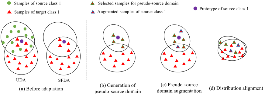
Figure 1: The motivation of the proposed method. (a) Although there are no source samples, we find that the target samples near the source prototypes can be used to represent the source domain. Thus, (b) PS firstly generates a pseudo-source domain by selecting such target samples. Then, (c) PS enlarges this pseudo-source domain using data augmentation. Lastly, (d) PS performs distribution alignment with four losses. Among them, the domain adversarial loss is introduced to reduce the distribution shift.

Based on the above analysis, we aim to reduce domain shift to further improve the performance of SFDA. Although there are no source samples, the trained model can retain and reflect original data distribution information. As shown in Figure 1(a), assuming there are some source samples, it is obvious that they are spread around the corresponding prototypes, where the class centers or weight vectors of the classifier can be regarded as the prototypes (Saito, Watanabe et al. 2018). Although there exists domain shift, we obverse that some target samples are also spread around the corresponding source prototypes and they are very similar to the source domain. Thus, these target samples could be used to approximate the source domain. We denote these samples as pseudo-source samples and the corresponding new domain as the pseudo-source domain. In other words, the target samples could be split into two disjoint parts, i.e., the pseudo-source samples and the remaining target samples. In such cases, reducing the distribution discrepancy across domains can be approximately achieved by minimizing the discrepancy between the pseudo-source samples and the remaining target samples. Although some UDA methods also split the target samples into two parts, such as easy samples and hard samples in (Pan et al. 2020), the goal is different. The method in (Pan et al. 2020) aims to reduce the intra-domain gap within the target domain while our method aims to generate pseudo-source samples for reducing the shift across domains.

Following the above idea, in this paper, we propose a method named Pseudo-Source domain based source-free domain adaptation (PS). Our method is composed of three steps. The first step is to generate a pseudo-source domain by selecting the target samples that are similar to the source domain. As the number of the samples in the pseudo-source domain is smaller than the number of the remaining target samples, the second step is to augment the pseudo-source domain to enlarge this new domain for better adaptation. The third step is to perform distribution alignment with four proposed losses. During distribution alignment, PS also adopts pseudo-label based strategy to train the model. Notably, among four losses, a domain adversarial loss is introduced between the pseudo-source domain and the remaining target domain to decrease the distribution discrepancy across domains. To sum up, our principal contributions are summarized as follows:

• We are the first to generate a pseudo-source domain from the target samples and perform distribution alignment for SFDA, such that the domain discrepancy across domains can be reduced even without source samples.

• We propose a novel method, which generates and augments the pseudo-source domain and then performs distribution alignment for explicit adaptation.

• Extensive experiments are conducted and the results show that the proposed method achieves better performance than state-of-the-art methods.

Related Work

Unsupervised Domain Adaptation

A classical domain adaptation theory (Ben-David et al. 2009) indicates that it is crucial to reduce the distribution discrepancy across domains to achieve better adaptation. Based on this theory, many domain adaptation methods have been proposed and they are divided into moment matching and adversarial domain adaptation. The goal of the former is to reduce the statistical distribution discrepancy across domains. The widely used statistical measurements include the first-order moment (Long et al. 2015; Kang, Jiang et al. 2019), the second-order moment(Sun, Feng, and Saenko 2016), high-order moment(Chen et al. 2020a; Zellinger et al. 2017) and other statistical measurements (Long et al. 2017; Li et al. 2020; Shen et al. 2018).

Adversarial domain adaptation, which is inspired by generative adversarial network (Goodfellow, Pouget-Abadie et al. 2014), reduces the distribution discrepancy in an adversarial manner. DANN (Ganin et al. 2016) introduces a domain discriminator which plays a min-max game with the feature extractor by the domain adversarial loss. MCD (Saito, Watanabe et al. 2018) introduces two classifiers as a discriminator to play a min-max game with the feature extractor such that the source samples are pushed into the support of the target domain. Considering practical multi-class problem, MDD (Zhang, Liu et al. 2019) proposes a margin-based theory, and a new method based on this theory is proposed. Following methods (Cicek and Soatto 2019; Chen et al. 2020b) adopt the multi-class discriminator which considers the domain and class information simultaneously. However, previous UDA methods cannot be applied to SFDA directly due to the absence of source samples.

Source-Free Domain Adaptation

The source samples are unavailable in source-free domain adaptation due to data privacy and security. However, a model trained by the source samples is given and the goal is to adapt the trained model to the target domain. Some methods adopt pseudo-label based strategy. SHOT (Liang, Hu et al. 2020) learns a target-specific feature extraction module by self-supervised pseudo-labeling together with information maximization and implicitly aligns representations of the target domain to the source model. CPGA (Qiu et al. 2021) proposes to utilize the hidden knowledge in the source model and exploits it to generate source avatar prototypes as well as target pseudo-labels for domain alignment. PrDA (Kim, Cho et al. 2020) progressively updates the target model in a self-learning manner by leveraging a pre-trained model from the source domain, such that the pseudo-labels would become more accurate for better adaptation.

Some methods adopt generative adversarial nets (GAN) to generate more samples. MA (Li, Jiao et al. 2020) proposes to generate target-style data with a class conditional generative adversarial net. SDDA (Kurmi, Subramanian, and Namboodiri 2021) treats the trained classifier as an energy-based model to learn the data distribution along with a generative adversarial net for generating source-like samples. Besides, some works explore source-free domain adaptation under different settings such as universal SFDA (Kundu et al. 2020) and multi-source SFDA (Ahmed et al. 2021; Feng et al. 2021). Moreover, Some works focus on different applications such as semantic segmentation (Liu, Zhang, and Wang 2021; Zhao et al. 2021) and object detection (Li et al. 2021). Although achieving remarkable progress, these methods do not explicitly reduce the distribution shift across domains.

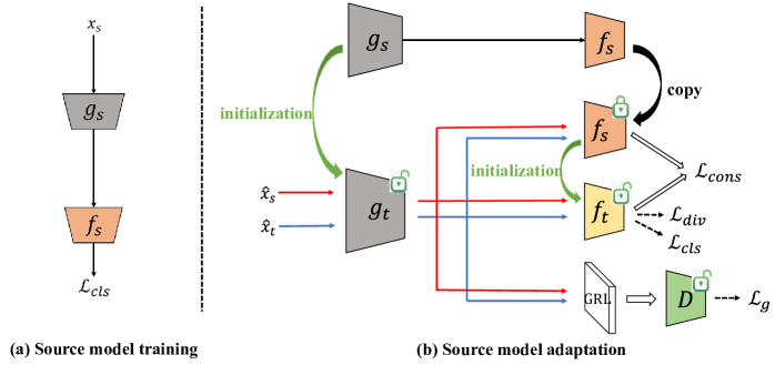
Figure 2: The model structure of the proposed method. $g_{s}$, $f_{s}$ and $g_{t}$, $f_{t}$ are the feature extractors and classifiers of the source model and target model, respectively. GRL is the gradient reversal layer and $D$ is the domain discriminator.

Problem Definition

In a vanilla UDA task, there are a labeled source domain $\mathcal{D}_{s}=\{x_{s}^{i},y_{s}^{i}\}_{i=1}^{n_{s}}$ and an unlabeled target domain $\mathcal{D}_{t}=\{x_{t}^{i}\}_{i=1}^{n_{t}}$, where $x_{s}^{i}\in\mathcal{X}_{s}$, $y_{s}^{i}\in\mathcal{Y}_{s}$, and $x_{t}^{i}\in\mathcal{X}_{t}$. The feature space and the label space are the same across domains, i.e., $\mathcal{X}_{s}=\mathcal{X}_{t}=\mathcal{R}^{d}$ and $\mathcal{Y}_{s}=\mathcal{Y}_{t}=\{1,2,...,K\}$. While the source samples and target samples are drawn from different distributions $P_{s}(x,y)$ and $P_{t}(x,y)$, i.e., $P_{s}(x,y)\neq P_{t}(x,y)$. In UDA, the goal is to train a model that can perform well in the target domain using both labeled source samples of $\mathcal{D}_{s}$ and unlabeled target samples of $\mathcal{D}_{t}$.

While in SFDA, the target domain can not access the source samples, but a model $F_{s}$ trained by the source samples is given. The goal of SFDA is to use the trained source model $F_{s}$ and unlabeled target samples of $\mathcal{D}_{t}$ to train a new model $F_{t}$, such that $F_{t}$ performs well in the target domain.

Method

The model structure of the proposed method is shown in Figure 2(b). The source trained model $F_{s}$ is composed of a feature extractor $g_{s}$ and a classifier $f_{s}$, i.e., $F_{s}(x)=f_{s}(g_{s}(x))$. The target model also contains a feature extractor $g_{t}$ and a classifier $f_{t}$, i.e., $F_{t}(x)=f_{t}(g_{t}(x))$. Besides, a domain discriminator $D$ is also introduced. To better transfer knowledge from the source domain to the target domain, the feature extractor $g_{t}$ of target model is initialized by the feature extractor $g_{s}$ of source model, and the target classifier $f_{t}$ is also initialized by the source classifier $f_{s}$. Note that the source classifier $f_{s}$ is fixed during training, while the target classifier $f_{t}$ would be updated. In the following subsections, we firstly introduce the training process of source model and then describe these training steps of the proposed method.

Training of Source Model

In SFDA setting, as is shown in Figure 2(a), a model $F_{s}:\mathcal{X}_{s}\rightarrow\mathcal{Y}_{s}$ is trained by the source samples and the trained model $F_{s}$ is delivered to the target domain. To further increase the discriminability of the source model, following previous work (Liang, Hu et al. 2020), PS adopts the label-smoothing technique to train the model as it encourages samples to lie in tight evenly separated clusters (Müller, Kornblith et al. 2019). The objective function is,

$$\mathcal{L}_{cls}^{s}(g_{s},f_{s};\mathcal{D}_{s})=$$ (1)

$$-\mathbb{E}_{(x_{s},y_{s})\in\mathcal{D}_{s}} \sum\nolimits_{k=1}^{K}q_{k}^{ls}\log\delta_{k}(f_{s}(g_{s}(x_{s})))$$

where $f_{s}(g_{s}(x_{s}))$ is the $K$-dimensional output of the source sample $x_{s}$. $q^{ls}_{k}=(1-\gamma)q_{k}^{s}+\gamma/K$ is the smoothed label and $\gamma$ is the smoothing parameter which is empirically set to 0.1. $\delta_{k}(\mathbf{a})=\frac{exp(a_{k})}{\sum_{i}exp(a_{i})}$ denotes the $k$-th element in the softmax output of a $K$-dimensional vector $\mathbf{a}$. $q^{s}$ is the one-of-$K$ encoding of $y_{s}$ where $q_{k}^{s}$ is ‘1’ for the correct class and ‘0’ for the rest.

Generation of Pseudo-Source Domain

As the source samples are not available in the target domain, conventional UDA methods can not be directly used to reduce the domain shift. Fortunately, we find that some target samples can be used to represent the source domain. Such samples are denoted as pseudo-source samples and constitute a new domain denoted as pseudo-source domain. This process can be regarded as dividing the samples in the target domain into two disjoint parts, where the first part is the pseudo-source domain, denoted as $\hat{\mathcal{D}}_{s}$, and the second part is the remaining target domain, denoted as $\hat{\mathcal{D}}_{t}$. It is obvious that $\hat{\mathcal{D}}_{s}\cap\hat{\mathcal{D}}_{t}=\varnothing$ and $\hat{\mathcal{D}}_{s}\cup\hat{\mathcal{D}}_{t}=\mathcal{D}_{t}$.

As is shown in Figure 1, the target samples near the source prototypes are similar to the source domain. The entropy criterion is widely used in UDA (Long, Cao et al. 2018; Pan et al. 2020) to evaluate the uncertainty of classifier prediction for a given sample. The lower the entropy is, the closer the sample is to the prototype. Thus, in this paper, PS adopts the entropy criterion to select the target samples that can be used to simulate the source domain. Given a trained source model $F_{s}$, all the target samples firstly pass the source model and then the entropy $H(x_{t})$ is calculated,

$$H(x_{t})=-\sum\nolimits_{k=1}^{K}\delta_{k}(f_{s}(g_{s}(x_{t})))\log\delta_{k}(f_{s}(g_{s}(x_{t})))$$ (2)

To generate a class-balanced pseudo-source domain, all the target samples are sorted in ascending order of entropy and PS selects samples from each class separately, i.e., the top $\alpha$ proportion of samples in each class are selected. As the samples in the target domain are unlabeled, the pseudo-labels are used instead. For the sample ${x}_{t}\in\mathcal{D}_{t}$, the pseudo-label $\hat{y}_{t}$ is obtained by

$$\hat{y}_{t}=\arg\max_{y\in\{1,...,K\}}f_{s}(g_{s}(x_{t}))$$ (3)

By this strategy, PS generates a class-balanced new domain and we experimentally find that $\alpha=0.1$ works well.

Pseudo-Source Domain Augmentation

Previous works have shown that the larger the source domain is, the better performance the model could get (Ganin et al. 2016; Kumar et al. 2018). However, the number of the samples in the pseudo-source domain $\hat{\mathcal{D}}_{s}$ is smaller than that in the remaining target domain $\hat{\mathcal{D}}_{t}$ (namely, $|\hat{\mathcal{D}}_{s}|:|\hat{\mathcal{D}}_{t}|\approx$ 1:9). Thus, PS enlarges the pseudo-source domain using data augmentation. In this work, mixup (Zhang et al. 2018) is choosen, as it is a simple yet effective supervised data augmentation method. Given two samples from the pseudo-source domain, e.g., $\hat{x}_{s}^{i},\hat{x}_{s}^{j}\in\hat{\mathcal{D}}_{s}$, whose pseudo-labels are obtained by Equ 3 and denoted as $\hat{y}_{s}^{i}$ and $\hat{y}_{s}^{j}$, PS augments the pseudo-source domain by mixing these two samples,

$$\begin{split}&\hat{x}_{s,aug}=\lambda\hat{x}_{s}^{i}+(1-\lambda)\hat{x}_{s}^{j}\\ &\hat{y}_{s,aug}=\lambda\hat{y}_{s}^{i}+(1-\lambda)\hat{y}_{s}^{j}\end{split}$$ (4)

where $\lambda\sim$ Beta($\beta$, $\beta$), for $\beta\in(0,\infty)$. The new domain which is composed of augmented pseudo-source samples is denoted as augmented domain $\hat{\mathcal{D}}_{aug}=\{\hat{x}_{s,aug},\hat{y}_{s,aug}\}_{i=1}^{n}$. And the domain that contains the original pseudo-source domain $\hat{\mathcal{D}}_{s}$ and the augmented source domain $\hat{\mathcal{D}}_{aug}$ is denoted as augmented pseudo-source domain $\hat{\mathcal{D}}_{s}^{aug}$, i.e. $\hat{\mathcal{D}}_{s}^{aug}=\hat{\mathcal{D}}_{s}\cup\hat{\mathcal{D}}_{aug}$. After adopting mixup, the dataset can be effectively enlarged.

Distribution Alignment

After generating and augmenting the pseudo-source domain, PS performs distribution alignment where pseudo-label based strategy is also used to train the model. In distribution alignment, four complementary losses are proposed for better adaptation in the target domain.

Classification loss

PS firstly trains the new model $F_{t}(x)$ to classify the samples in both the augmented pseudo-source domain and the remaining target domain correctly. Similar to previous work (Saito, Ushiku, and Harada 2017), training the model to classify the target samples with pseudo-labels could help the model capture the characteristics of the target domain. The objective function is

$$\mathcal{L}_{cls}(g_{t},f_{t};\hat{\mathcal{D}}_{s}^{aug},\hat{\mathcal{D}}_{t}) =\mathbb{E}_{(\hat{x}_{s},\hat{y}_{s})\sim\hat{\mathcal{D}}_{s}^{aug}}L(g_{t}(f_{t}(\hat{x}_{s})),\hat{y}_{s})$$ (5)

$$+\mathbb{E}_{(\hat{x}_{t},\hat{y}_{t})\sim\hat{\mathcal{D}}_{t}} L(f_{t}(g_{t}(\hat{x}_{t})),\hat{y}_{t})$$

where $L(\cdot,\cdot)$ is the cross-entropy loss. For the samples in $\hat{\mathcal{D}}_{t}$, the pseudo-labels obtained by Equ 3 may be incorrect as the entropy is very high. We incorporate the method in SHOT (Liang, Hu et al. 2020) to regenerate the pseudo-labels and the detail steps are shown in the supplementary materials.

Diversity loss

As there are only unlabeled samples in the remaining target domain, to avoid the collapse mode, PS adopts the information maximization (Gomes, Krause, and Perona 2010) to make the target outputs globally diverse,

$$\mathcal{L}_{div}(g_{t},f_{t};\hat{\mathcal{D}}_{t}) =\sum\nolimits_{k=1}^{K}p_{1,k}logp_{1,k}+\sum\nolimits_{k=1}^{K}p_{2,k}logp_{2,k}$$ (6)

$$=[D_{KL} (p_{1},\frac{1}{K}\mathbf{1}_{K})+D_{KL}(p_{2},\frac{1}{K}\mathbf{1}_{K})]-2logK,$$

where $\mathbf{1}_{K}$ is a $K$-dimensional vector with all ones, and $p_{1}=\mathbb{E}_{\hat{x}_{t}\in\hat{\mathcal{D}}_{t}}[\delta(f_{s}(g_{t}(\hat{x}_{t})))]$ and $p_{2}=\mathbb{E}_{\hat{x}_{t}\in\hat{\mathcal{D}}_{t}}[\delta(f_{t}(g_{t}(\hat{x}_{t})))]$ are the mean output embeddings of the whole target domain by classifiers $f_{s}$ and $f_{t}$, respectively. $p_{1,k}$ and $p_{2,k}$ are the $k$-th element of the outputs of $f_{s}$ and $f_{t}$, respectively. With the fair diversity-promoting objective $\mathcal{L}_{div}$, the learned model can circumvent the trivial solution where all unlabeled data have the same one-hot encoding.

Algorithm 1 Training of PS

0:  Trained source model $F_{s}$ composed of $g_{s}$ and $f_{s}$, unlabeled target samples of $\mathcal{D}_{t}$, batchsize $B$, and proportion $\alpha$.

0:  Trained target model $F_{t}$ composed of $g_{t}$ and $f_{t}$.

1:  Initialization: Initialize $g_{t}$ with $g_{s}$, initialize $f_{t}$ with $f_{s}$.

2:  repeat

3:     Sample a minibatch of size $B$ from $\mathcal{D}_{t}$.

4:     Generation: Sort all the target samples with the entropy calculated by Equ 2 in each class, and split samples of the top $\alpha$ proportion as $\hat{\mathcal{D}}_{s}$ and the remaining samples as $\hat{\mathcal{D}}_{t}$.

5:     Augmentation: Augment the samples in pseudo-source domains $\hat{\mathcal{D}}_{s}$ by Equ 4 to get augmented pseudo-source domain $\hat{\mathcal{D}}_{s}^{aug}$.

6:     Alignment:

7:      1) Train the feature extractor $g_{t}$ and domain discriminator $D$ by Equ 9.

8:      2) Train the feature extractor $g_{t}$ and the classifier $f_{t}$ by Equ 10.

9:  until Maximum iteration or loss convergence

Constrain loss

the source classifier $f_{s}$ is kept unchanged during training. As the source classifier $f_{s}$ could retain the learned knowledge from the source domain, PS aims to force the learned target classifier $f_{t}$ to be not far away from the source classifier $f_{s}$. Such strategy is also used in continuous learning and incremental learning (Li and Hoiem 2018; Parisi et al. 2019). Specially, PS trains the features extractor $g_{t}$ to make the outputs of these two classifiers similar,

$$\begin{split}\mathcal{L}_{\mathrm{cons}}(g_{t};\hat{\mathcal{D}}_{t})=&\mathbb{E}_{\hat{x}_{t}\sim\hat{\mathcal{D}}_{t}}[L(f_{s}(g_{t}(\hat{x}_{t})),f_{t}(g_{t}(\hat{x}_{t})))\\ &+L(f_{t}(g_{t}(\hat{x_{t}})),f_{s}(g_{t}(\hat{x}_{t})))]\end{split}$$ (7)

Domain adversarial loss

Though achieving remarkable progress (Liang, Hu et al. 2020; Li, Jiao et al. 2020), previous SFDA methods do not explicitly reduce the distribution shift across domains. So in this work, PS aims to learn domain-invariant features in an adversarial manner. Similar to previous work (Ganin and Lempitsky 2015), a domain discriminator $D$ is introduced to distinguish the augmented pseudo-source domain $\hat{\mathcal{D}}_{s}^{aug}$ from the remaining target domain $\hat{\mathcal{D}}_{t}$. While the feature extractor $g_{t}$ is trained to confuse the domain discriminator $D$. The adversarial objective function is,

$$\mathcal{L}_{g}(g_{t},D;\hat{\mathcal{D}}_{s}^{aug},\hat{\mathcal{D}}_{t}) =\mathbb{E}_{\hat{x}_{s}\sim\hat{\mathcal{D}}_{s}^{aug}}[\log D(g_{t}(\hat{x}_{s}))]$$ (8)

$$+\mathbb{E}_{\hat{x}_{t}\sim\hat{\mathcal{D}}_{t}}[\log(1-D(g_{t}(\hat{x}_{t})))]$$

Training Steps

In this subsection, we summarize the training steps of PS. Combining the above objectives discussed together, the overall objective is:

$$\min_{g_{t}}\max_{D}\mathcal{L}_{cons}(g_{t})+\lambda_{g}\mathcal{L}_{g}(g_{t},D)\vspace{-2mm}$$ (9)

$$\min_{g_{t},f_{t}}\mathcal{L}_{div}(g_{t},f_{t})+\lambda_{c}\mathcal{L}_{cls}(g_{t},f_{t})$$ (10)

Following the previous method (Ganin and Lempitsky 2015), the min-max training procedure in Equ 9 is accomplished by applying a Gradient Reversal Layer (GRL). GRL behaves as the identity function during the forward propagation and inverts the gradient sign during the backward propagation, hence driving the parameters to maximize the output loss. During the distribution alignment, the model is trained by the losses in Equ 9 and Equ 10 alternatively.

Remark: In our method, PS performs pseudo-source domain generation, pseudo-source domain augmentation and distribution alignment in an alternative manner. All three steps are employed in a minibatch of size $B$. The pseudo-source code is shown in Algorithm 1.

Method (Source$\to$Target)	Source-free	S$\to$M	U$\to$M	M$\to$U	Avg.
Source-only	✗	67.1$\pm$0.6	69.6$\pm$3.8	82.2$\pm$0.8	73.0
ADDA	✗	76.0$\pm$1.8	90.1$\pm$0.8	89.4$\pm$0.2	85.2
ADR	✗	95.0$\pm$1.9	93.1$\pm$1.3	93.2$\pm$2.5	93.8
CDAN+E	✗	89.2	98.0	95.6	94.3
CyCADA	✗	90.4$\pm$0.4	96.5$\pm$0.1	95.6$\pm$0.4	94.2
rRevGrad+CAT	✗	98.8$\pm$0.0	96.0$\pm$0.9	94.0$\pm$0.7	96.3
SWD	✗	98.9$\pm$0.1	97.1$\pm$0.1	98.1$\pm$0.1	98.0
SHOT-IM	✓	89.6$\pm$5.0	96.8$\pm$0.4	91.9$\pm$0.4	92.8
SHOT	✓	98.9$\pm$0.0	98.4$\pm$0.6	98.0$\pm$0.2	98.4
PS (ours)	✓	99.0$\pm$0.1	98.6$\pm$0.0	98.2$\pm$0.2	98.6
Target-supervised (Oracle)		99.4$\pm$0.1	99.4$\pm$0.1	98.0$\pm$0.1	98.8

Table 1: Classification accuracies (%) on Digits dataset.

Experiments

Method	Source-free	Ar$\rightarrow$Cl	Ar$\rightarrow$Pr	Ar$\rightarrow$Rw	Cl$\rightarrow$Ar	Cl$\rightarrow$Pr	Cl$\rightarrow$Rw	Pr$\rightarrow$Ar	Pr$\rightarrow$Cl	Pr$\rightarrow$Rw	Rw$\rightarrow$Ar	Rw$\rightarrow$Cl	Rw$\rightarrow$Pr	Avg.
ResNet-50	✗	34.9	50.0	58.0	37.4	41.9	46.2	38.5	31.2	60.4	53.9	41.2	59.9	46.1
MCD	✗	48.9	68.3	74.6	61.3	67.6	68.8	57.0	47.1	75.1	69.1	52.2	79.6	64.1
CDAN	✗	50.7	70.6	76.0	57.6	70.0	70.0	57.4	50.9	77.3	70.9	56.7	81.6	65.8
MDD	✗	54.9	73.7	77.8	60.0	71.4	71.8	61.2	53.6	78.1	72.5	60.2	82.3	68.1
BNM	✗	52.3	73.9	80.0	63.3	72.9	74.9	61.7	49.5	79.7	70.5	53.6	82.2	67.9
BDG	✗	51.5	73.4	78.7	65.3	71.5	73.7	65.1	49.7	81.1	74.6	55.1	84.8	68.7
SRDC	✗	52.3	76.3	81.0	69.5	76.2	78.0	68.7	53.8	81.7	76.3	57.1	85.0	71.3
PrDA	✓	48.4	73.4	76.9	64.3	69.8	71.7	62.7	45.3	76.6	69.8	50.5	79.0	65.7
SHOT-IM	✓	55.4	76.6	80.4	66.9	74.3	75.4	65.6	54.8	80.7	73.7	58.4	83.4	70.5
BAIT	✓	57.4	77.5	82.4	68.0	77.2	75.1	67.1	55.5	81.9	73.9	59.5	84.2	71.6
CPGA	✓	59.3	78.1	79.8	65.4	75.5	76.4	65.7	58.0	81.0	72.0	64.4	83.3	71.6
SHOT	✓	57.1	78.1	81.5	68.0	78.2	78.1	67.4	54.9	82.2	73.3	58.8	84.3	71.8
PS (ours)	✓	57.8	77.3	81.2	68.4	76.9	78.1	67.8	57.3	82.1	75.2	59.1	83.4	72.1

Table 2: Classification accuracies (%) on the Office-Home dataset (ResNet-50).

Method	Source-free	plane	bicycle	bus	car	horse	knife	mcycl	person	plant	sktbrd	train	truck	Per-class
ResNet-101	✗	55.1	53.3	61.9	59.1	80.6	17.9	79.7	31.2	81.0	26.5	73.5	8.5	52.4
CDAN	✗	85.2	66.9	83.0	50.8	84.2	74.9	88.1	74.5	83.4	76.0	81.9	38.0	73.9
SAFN	✗	93.6	61.3	84.1	70.6	94.1	79.0	91.8	79.6	89.9	55.6	89.0	24.4	76.1
SWD	✗	90.8	82.5	81.7	70.5	91.7	69.5	86.3	77.5	87.4	63.6	85.6	29.2	76.4
TPN	✗	93.7	85.1	69.2	81.6	93.5	61.9	89.3	81.4	93.5	81.6	84.5	49.9	80.4
PAL	✗	90.9	50.5	72.3	82.7	88.3	88.3	90.3	79.8	89.7	79.2	88.1	39.4	78.3
MCC	✗	88.7	80.3	80.5	71.5	90.1	93.2	85.0	71.6	89.4	73.8	85.0	36.9	78.8
CoSCA	✗	95.7	87.4	85.7	73.5	95.3	72.8	91.5	84.8	94.6	87.9	87.9	36.8	82.9
PrDA	✓	86.9	81.7	84.6	63.9	93.1	91.4	86.6	71.9	84.5	58.2	74.5	42.7	76.7
SHOT-IM	✓	93.7	86.4	78.7	50.7	91.0	93.5	79.0	78.3	89.2	85.4	87.9	51.1	80.4
MA	✓	94.8	73.4	68.8	74.8	93.1	95.4	88.6	84.7	89.1	84.7	83.5	48.1	81.6
BAIT	✓	93.7	83.2	84.5	65.0	92.9	95.4	88.1	80.8	90.0	89.0	84.0	45.3	82.7
SHOT	✓	94.3	88.5	80.1	57.3	93.1	94.9	80.7	80.3	91.5	89.1	86.3	58.2	82.9
PS (ours)	✓	95.3	86.2	82.3	61.6	93.3	95.7	86.7	80.4	91.6	90.9	86.0	59.5	84.1

Table 3: Classification accuracies (%) on the large-scale VisDA dataset (ResNet-101).

Datasets

We conduct experiments on three benchmark datasets: (1) Digits is a standard dataset that focuses on digit recognition. We follow the protocol of (Hoffman, Tzeng et al. 2018) and choose three subsets: SVHN (S), MNIST (M), and USPS (U). (2) Office-Home (Venkateswara, Eusebio et al. 2017) is a widely used dataset, which contains four domains: Artistic images (Ar), Clip Art (Cl), Product images (Pr) and Real-world images (Rw). Each domain has 65 categories. (3) VisDA (Peng, Usman et al. 2017) is a challenging large-scale dataset that concentrates on the synthesis-to-real object recognition task. The source domain contains 152k synthetic images while the target domain has 55k real object images with 12 classes.

Baselines

We compare PS with three types of baselines: (1) Source-only: ResNet (He, Zhang et al. 2016) or LeNet (LeCun et al. 1998); (2) UDA methods: ADDA (Tzeng et al. 2017), ADR (Saito et al. 2018), MCD (Saito, Watanabe et al. 2018), CDAN (Long, Cao et al. 2018), CyDADA (Hoffman, Tzeng et al. 2018), SAFN (Xu, Li et al. 2019), SWD (Lee et al. 2019a), TPN (Pan, Yao et al. 2019), CAT (Deng, Luo, and Zhu 2019), MDD (Zhang, Liu et al. 2019), SWD (Lee et al. 2019b), BDG (Yang, Xia et al. 2020), PAL (Hu, Liang et al. 2020), MCC (Jin, Wang et al. 2020), BNM (Cui, Wang et al. 2020), CoSCA (Dai, Cheng et al. 2020) and SRDC (Tang, Chen, and Jia 2020); (3) SFDA methods: PrDA (Kim, Cho et al. 2020), SHOT (Liang, Hu et al. 2020), MA (Li, Jiao et al. 2020), BAIT (Yang, Wang et al. 2020) and CPGA (Qiu et al. 2021).

Implementation Details

Our method is implemented based on PyTorch. For a fair comparison, we report the results of all baselines in the corresponding papers. For the network architecture, a ResNet (He, Zhang et al. 2016) pre-trained on ImageNet is adopted as the feature extractor of all methods for the object recognition task. For the digit recognition task, we use the same architectures with CDAN (Long, Cao et al. 2018), namely, the classical LeNet-5 (LeCun et al. 1998) network is utilized for USPS$\leftrightarrow$ MNIST and a variant of LeNet is utilized for SVHN$\rightarrow$ MNIST. Following (Liang, Hu et al. 2020), we replace the original fully connected (FC) layer with a task-specific FC layer followed by a weight normalization layer. We train the model using SGD optimizer with momentum 0.9 and weight decay $5e^{-4}$. The learning rate of the domain discriminator and the classifier is 10 times that of the feature extractor, where the former is set to be $1e^{-4}$ for Digits and $1e^{-5}$ for Office-Home and VisDA. Besides, the number of epoch is set to be 200, 800, and 60 for Digits, Office-Home, and VisDA, respectively. For hyper-parameters, we set $\alpha$ to be 0.1 for all datasets and batchsize $B$ to be 500, 658, and 128 for Digits, Office-Home, and VisDA, respectively. We set $\lambda_{g}=0.5$ and $\lambda_{c}=1$ for all datasets except $\lambda_{c}=0.3$ for Office-Home.

Results

For Digits recognition, as shown in Table 1, PS obtains the best mean accuracies for each task and outperforms prior work in terms of the average accuracy. The proposed method performs better than SHOT and SHOT-IM, as PS could take the distribution discrepancy into consideration. It is noticed that both PS and SHOT achieve better results than the supervised learning for task M$\rightarrow$U, which is because that the large source domain MNIST contains more useful information suitable for the small target domain USPS. For Office-Home dataset, as shown in Table 2, the proposed PS achieves the best performance compared with other SFDA methods w.r.t. the average accuracy over four transfer tasks. Moreover, our method shows its superiority in the task of Cl$\rightarrow$Ar and Rw$\rightarrow$Ar and comparable results on the other tasks. Moreover, from Table 3, PS outperforms all the state-of-the-art methods on the more challenging large-scale dataset VisDA. Specifically, PS gets the best accuracy in the six categories and obtains comparable results in others. Note that for these three datasets, even compared with the state-of-the-art methods using source data (e.g.,SWD, SRDC, CoSCA), our PS is able to obtain a competitive result as well, which shows that PS could make a better adaptation across domains.

Insight Analysis

Ablation of selection criterion of pseudo-source samples

To study the selection criterion of pseudo-source samples, we compare the model with two criterion, i.e., entropy criterion (our method) and random selection (with the same proportion in each class). As shown in Table 4, PS with entropy criterion (line 3) outperforms random selection (line 1) by 0.5% in VisDA dataset. We also find that random selection achieves better results than some SFDA method, as such split strategy can be regraded as reducing the intra-domain discrepancy within the target domain (Pan et al. 2020).

Method	Digits	VisDA
Random selection with mixup	98.4	83.6
Entropy criterion without mixup	98.4	83.4
Entropy criterion with mixup (ours)	98.6	84.1

Table 4: Ablation study of generation and augmentation on Digits and VisDA dataset.

Ablation of pseudo-source domain augmentation

To explore the impact of data augmentation, we conduct experiments with and without mixup. From Table 4, compared with other SFDA method, both settings achieve better performance. In other words, even without mixup (line 2), our method could also get comparable results. With mixup (line 3), the model gets a better performance.

Ablation of loss functions

To investigate the losses in distribution alignment, the quantitative results of the model optimized by different losses are shown in Table 5. When only using classification loss $\mathcal{L}_{cls}$, the model gets better performance than source-only model as the self-training based strategy could perform implicit alignment to the source model. Besides, our model is able to further improve the performance when introducing the losses $\mathcal{L}_{div}$ and $\mathcal{L}_{con}$. Such a result verifies the benefit of encouraging diverse outputs and retaining knowledge of source domain. Finally, a combination of all losses can achieve the best results.

Distribution distance

The $\mathcal{A}$-distance is a measure of domain discrepancy (Ben-David et al. 2009), defined as $d_{A}=2(1-2\epsilon)$, where $\epsilon$ is the error rate of a domain classifier trained to discriminate source domain and target domain. To show the true distribution distance across domains, we compute the $\mathcal{A}$-distance using both true source samples and target samples. Note that the source samples are only used for computing $\mathcal{A}$-distance, not used for training. Results on tasks M$\rightarrow$U are shown in Figure 3. SHOT implicitly aligns representations of the target domain to the source model, thus getting a smaller distance than source-only method. PS could get smaller $\mathcal{A}$-distance than SHOT by further reducing the domain shift explicitly.

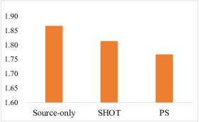
Figure 3: $\mathcal{A}$-distance.

Method	Digits	VisDA
Source-only	79.3	46.6
$\mathcal{L}_{cls}$	98.3	77.6
$\mathcal{L}_{cls}$ + $\mathcal{L}_{div}$	98.3	78.4
$\mathcal{L}_{cls}$ + $\mathcal{L}_{div}$ + $\mathcal{L}_{cons}$	98.4	83.0
Ours (all)	98.6	84.1

Table 5: Ablation of losses on Digits and VisDA dataset.

Parameter sensitivity

In this subsection, we evaluate the sensitivity of two hyper-parameters batchsize $B$ and proportion $\alpha$ on Digits. As shown in Figure 4(a), the results demonstrate that our method is non-sensitive to the batchsize. Although PS generates and augments the pseudo-source domain within a minibatch instead of the whole domain, it could achieve stable results because many random minibatches can be seen as an approximation of the whole domain. The results in Figure 4(b) show that with the increasing of $\alpha$, the performance grows firstly and then drops. The reason is that a small proportion would lead to a small number of pseudo-source samples and a large proportion would select some samples not similar to the source domain into the pseudo-source domain. We experimentally find $\alpha=0.1$ works well.

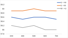
(a) Sensitivity of batchsize $B$

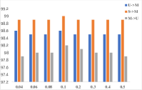
(b) Sensitivity of proportion $\alpha$

Figure 4: Results of parameter sensitivity.

Embedding visualization

Figure 5(a) and (b) show the t-SNE visualization of the features from the pseudo-source domain and the remaining target domain for task M$\rightarrow$U (10 classes) before and after alignment, respectively. Before alignment, there exists large distribution shift between the pseudo-source domain and the remaining target domain. While after alignment the distribution shift is reduced and the features of target samples have become discriminative, thus, the samples can be easily classified by the classifier.

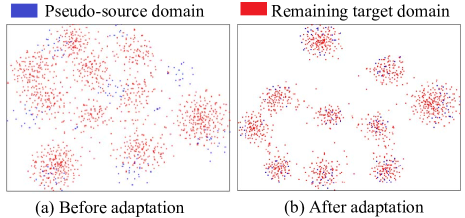
Figure 5: t-SNE visualization for features from the pseudo-source domain and the remaining target domain.

Conclusions

In this paper, we focus on source-free domain adaptation, where only a trained source model and unlabeled target samples are given. Considering that previous SFDA methods do not explicitly reduce the distribution shift across domains, we propose a novel method to reduce the shift explicitly. To be specific, we find that some target samples can be used to represent the source domain and the new domain is denoted as pseudo-source domain. The proposed method firstly generates and augments the pseudo-source domain and then employs distribution alignment between the pseudo-source domain and the remaining target domain. Thus, the domain shift can be reduced. Extensive experiments on three datasets show that our method outperforms the state-of-the-art methods.

References

- Ahmed et al. (2021) Ahmed, S. M.; Raychaudhuri, D. S.; Paul, S.; Oymak, S.; and Roy-Chowdhury, A. 2021. Unsupervised Multi-source Domain Adaptation Without Access to Source Data. CVPR .
- Ben-David et al. (2009) Ben-David, S.; Blitzer, J.; Crammer, K.; Kulesza, A.; Pereira, F. C.; and Vaughan, J. W. 2009. A theory of learning from different domains. Machine Learning 79: 151–175.
- Chen et al. (2020a) Chen, C.; Fu, Z.; Chen, Z.; Jin, S.; Cheng, Z.; Jin, X.; and Hua, X. 2020a. HoMM: Higher-order Moment Matching for Unsupervised Domain Adaptation. In AAAI.
- Chen et al. (2020b) Chen, Q.; Du, Y.; Tan, Z.; Zhang, Y.; and Wang, C.-J. 2020b. Unsupervised Domain Adaptation with Joint Domain-Adversarial Reconstruction Networks. In ECML/PKDD.
- Cicek and Soatto (2019) Cicek, S.; and Soatto, S. 2019. Unsupervised Domain Adaptation via Regularized Conditional Alignment. 2019 IEEE/CVF International Conference on Computer Vision (ICCV) 1416–1425.
- Cui, Wang et al. (2020) Cui, S.; Wang, S.; et al. 2020. Towards Discriminability and Diversity: Batch Nuclear-Norm Maximization Under Label Insufficient Situations. CVPR .
- Dai, Cheng et al. (2020) Dai, S.; Cheng, Y.; et al. 2020. Contrastively Smoothed Class Alignment for Unsupervised Domain Adaptation. In ACCV.
- Deng, Luo, and Zhu (2019) Deng, Z.; Luo, Y.; and Zhu, J. 2019. Cluster Alignment With a Teacher for Unsupervised Domain Adaptation. 2019 IEEE/CVF International Conference on Computer Vision (ICCV) 9943–9952.
- Feng et al. (2021) Feng, H.; You, Z.; Chen, M.; Zhang, T.-Y.; Zhu, M.; Wu, F.; Wu, C.; and Chen, W. 2021. KD3A: Unsupervised Multi-Source Decentralized Domain Adaptation via Knowledge Distillation. ICML .
- Ganin and Lempitsky (2015) Ganin, Y.; and Lempitsky, V. 2015. Unsupervised domain adaptation by backpropagation. In ICML.
- Ganin et al. (2016) Ganin, Y.; Ustinova, E.; Ajakan, H.; Germain, P.; Larochelle, H.; Laviolette, F.; Marchand, M.; and Lempitsky, V. S. 2016. Domain-Adversarial Training of Neural Networks. J. Mach. Learn. Res. 17: 59:1–59:35.
- Gomes, Krause, and Perona (2010) Gomes, R.; Krause, A.; and Perona, P. 2010. Discriminative Clustering by Regularized Information Maximization. In NIPS.
- Goodfellow, Pouget-Abadie et al. (2014) Goodfellow, I. J.; Pouget-Abadie, J.; et al. 2014. Generative Adversarial Networks. In NeruIPS.
- He, Zhang et al. (2016) He, K.; Zhang, X.; et al. 2016. Deep Residual Learning for Image Recognition. CVPR .
- Hoffman, Tzeng et al. (2018) Hoffman, J.; Tzeng, E.; et al. 2018. CyCADA: Cycle-Consistent Adversarial Domain Adaptation. In ICML.
- Hu, Liang et al. (2020) Hu, D.; Liang, J.; et al. 2020. PANDA: Prototypical Unsupervised Domain Adaptation. ArXiv .
- Jin, Wang et al. (2020) Jin, Y.; Wang, X.; et al. 2020. Minimum Class Confusion for Versatile Domain Adaptation. In ECCV.
- Kang, Jiang et al. (2019) Kang, G.; Jiang, L.; et al. 2019. Contrastive Adaptation Network for Unsupervised Domain Adaptation. CVPR .
- Kim, Cho et al. (2020) Kim, Y.; Cho, D.; et al. 2020. Progressive Domain Adaptation from a Source Pre-trained Model. ArXiv .
- Kumar et al. (2018) Kumar, A.; Sattigeri, P.; Wadhawan, K.; Karlinsky, L.; Feris, R.; Freeman, W.; and Wornell, G. 2018. Co-regularized Alignment for Unsupervised Domain Adaptation. NeurIPS .
- Kundu et al. (2020) Kundu, J. N.; Venkat, N.; RahulM., V.; and Babu, R. V. 2020. Universal Source-Free Domain Adaptation. 2020 IEEE/CVF Conference on Computer Vision and Pattern Recognition (CVPR) 4543–4552.
- Kurmi, Subramanian, and Namboodiri (2021) Kurmi, V.; Subramanian, V. K.; and Namboodiri, V. P. 2021. Domain Impression: A Source Data Free Domain Adaptation Method. 2021 IEEE Winter Conference on Applications of Computer Vision (WACV) 615–625.
- LeCun et al. (1998) LeCun, Y.; Bottou, L.; Bengio, Y.; and Haffner, P. 1998. Gradient-based learning applied to document recognition.
- Lee et al. (2019a) Lee, C.-Y.; Batra, T.; Baig, M. H.; and Ulbricht, D. 2019a. Sliced wasserstein discrepancy for unsupervised domain adaptation. In CVPR.
- Lee et al. (2019b) Lee, C.-Y.; Batra, T.; Baig, M. H.; and Ulbricht, D. 2019b. Sliced Wasserstein Discrepancy for Unsupervised Domain Adaptation. 2019 IEEE/CVF Conference on Computer Vision and Pattern Recognition (CVPR) 10277–10287.
- Li et al. (2020) Li, J.; Chen, E.; Ding, Z.; Zhu, L.; Lu, K.; and Shen, H. T. 2020. Maximum Density Divergence for Domain Adaptation. IEEE transactions on pattern analysis and machine intelligence .
- Li, Jiao et al. (2020) Li, R.; Jiao, Q.; et al. 2020. Model adaptation: Unsupervised domain adaptation without source data. In CVPR.
- Li et al. (2021) Li, X.; Chen, W.; Xie, D.; Yang, S.; Yuan, P.; Pu, S.; and Zhuang, Y. 2021. A Free Lunch for Unsupervised Domain Adaptive Object Detection without Source Data. In AAAI.
- Li and Hoiem (2018) Li, Z.; and Hoiem, D. 2018. Learning without Forgetting. IEEE Transactions on Pattern Analysis and Machine Intelligence 40: 2935–2947.
- Liang, Hu et al. (2020) Liang, J.; Hu, D.; et al. 2020. Do We Really Need to Access the Source Data? Source Hypothesis Transfer for Unsupervised Domain Adaptation. In ICML.
- Liu, Zhang, and Wang (2021) Liu, Y.; Zhang, W.; and Wang, J. 2021. Source-Free Domain Adaptation for Semantic Segmentation. CVPR .
- Long et al. (2015) Long, M.; Cao, Y.; Wang, J.; and Jordan, M. I. 2015. Learning Transferable Features with Deep Adaptation Networks. ICML .
- Long, Cao et al. (2018) Long, M.; Cao, Z.; et al. 2018. Conditional adversarial domain adaptation. In NeruIPS.
- Long et al. (2017) Long, M.; Zhu, H.; Wang, J.; and Jordan, M. I. 2017. Deep Transfer Learning with Joint Adaptation Networks. In ICML.
- Müller, Kornblith et al. (2019) Müller, R.; Kornblith, S.; et al. 2019. When Does Label Smoothing Help? In NeurIPS.
- Pan et al. (2020) Pan, F.; Shin, I.; Rameau, F.; Lee, S.; and Kweon, I. 2020. Unsupervised Intra-Domain Adaptation for Semantic Segmentation Through Self-Supervision. 2020 IEEE/CVF Conference on Computer Vision and Pattern Recognition (CVPR) 3763–3772.
- Pan and Yang (2010) Pan, S. J.; and Yang, Q. 2010. A Survey on Transfer Learning. IEEE Transactions on Knowledge and Data Engineering 22: 1345–1359.
- Pan, Yao et al. (2019) Pan, Y.; Yao, T.; et al. 2019. Transferrable prototypical networks for unsupervised domain adaptation. In CVPR.
- Parisi et al. (2019) Parisi, G. I.; Kemker, R.; Part, J. L.; Kanan, C.; and Wermter, S. 2019. Continual Lifelong Learning with Neural Networks: A Review. Neural networks 113: 54–71.
- Peng, Usman et al. (2017) Peng, X.; Usman, B.; et al. 2017. VisDA: The Visual Domain Adaptation Challenge. ArXiv .
- Qiu et al. (2021) Qiu, Z.; Zhang, Y.; Lin, H.; Niu, S.; Liu, Y.; Du, Q.; and Tan, M. 2021. Source-free Domain Adaptation via Avatar Prototype Generation and Adaptation. IJCAI .
- Ren et al. (2015) Ren, S.; He, K.; Girshick, R. B.; and Sun, J. 2015. Faster R-CNN: Towards Real-Time Object Detection with Region Proposal Networks. IEEE Transactions on Pattern Analysis and Machine Intelligence 39: 1137–1149.
- Saito, Ushiku, and Harada (2017) Saito, K.; Ushiku, Y.; and Harada, T. 2017. Asymmetric Tri-training for Unsupervised Domain Adaptation. In ICML.
- Saito et al. (2018) Saito, K.; Ushiku, Y.; Harada, T.; and Saenko, K. 2018. Adversarial Dropout Regularization. ICLR .
- Saito, Watanabe et al. (2018) Saito, K.; Watanabe, K.; et al. 2018. Maximum classifier discrepancy for unsupervised domain adaptation. In CVPR.
- Shen et al. (2018) Shen, J.; Qu, Y.; Zhang, W.; and Yu, Y. 2018. Wasserstein Distance Guided Representation Learning for Domain Adaptation. In AAAI.
- Sun, Feng, and Saenko (2016) Sun, B.; Feng, J.; and Saenko, K. 2016. Return of Frustratingly Easy Domain Adaptation. In AAAI.
- Tang, Chen, and Jia (2020) Tang, H.; Chen, K.; and Jia, K. 2020. Unsupervised Domain Adaptation via Structurally Regularized Deep Clustering. In CVPR.
- Tzeng et al. (2017) Tzeng, E.; Hoffman, J.; Saenko, K.; and Darrell, T. 2017. Adversarial Discriminative Domain Adaptation. CVPR .
- Venkateswara, Eusebio et al. (2017) Venkateswara, H.; Eusebio, J.; et al. 2017. Deep Hashing Network for Unsupervised Domain Adaptation. CVPR .
- Xu, Li et al. (2019) Xu, R.; Li, G.; et al. 2019. Larger norm more transferable: An adaptive feature norm approach for unsupervised domain adaptation. In ICCV.
- Yang, Xia et al. (2020) Yang, G.; Xia, H.; et al. 2020. Bi-Directional Generation for Unsupervised Domain Adaptation. In AAAI.
- Yang, Wang et al. (2020) Yang, S.; Wang, Y.; et al. 2020. Unsupervised Domain Adaptation without Source Data by Casting a BAIT. ArXiv .
- Zellinger et al. (2017) Zellinger, W.; Grubinger, T.; Lughofer, E.; Natschläger, T.; and Saminger-Platz, S. 2017. Central Moment Discrepancy (CMD) for Domain-Invariant Representation Learning. ICLR .
- Zhang et al. (2018) Zhang, H.; Cissé, M.; Dauphin, Y.; and Lopez-Paz, D. 2018. mixup: Beyond Empirical Risk Minimization. ICLR .
- Zhang, Liu et al. (2019) Zhang, Y.; Liu, T.; et al. 2019. Bridging Theory and Algorithm for Domain Adaptation. In ICML.
- Zhao et al. (2021) Zhao, Y.; Zhong, Z.; Luo, Z.; Lee, G. H.; and Sebe, N. 2021. Source-Free Open Compound Domain Adaptation in Semantic Segmentation. ArXiv abs/2106.03422.