New stabilized $P_{1}\times P_{0}$ finite element methods for nearly inviscid and incompressible flows

Abstract

This work proposes a new stabilized $P_{1}\times P_{0}$ finite element method for solving the incompressible Navier–Stokes equations. The numerical scheme is based on a reduced Bernardi–Raugel element with statically condensed face bubbles and is pressure-robust in the small viscosity regime. For the Stokes problem, an error estimate uniform with respect to the kinematic viscosity is shown. For the Navier–Stokes equation, the nonlinear convection term is discretized using an edge-averaged finite element method. In comparison with classical schemes, the proposed method does not require tunning of parameters and is validated for competitiveness on several benchmark problems in 2 and 3 dimensional space.

1 Introduction

Let $\Omega\subset\mathbb{R}^{d}$ be a bounded Lipschitz domain with $d\in\{2,3\}$. Let $\bm{u}:\Omega\rightarrow\mathbb{R}^{d}$ be the velocity field of a fluid occupying $\Omega$ and $p:\Omega\rightarrow\mathbb{R}$ denote its kinematic pressure. The dynamics of the incompressible fluid within $\Omega$ subject to the loads $\bm{f}\in L^{2}\big{(}0,T;[L^{2}(\Omega)]^{d}\big{)}$, $\bm{g}\in L^{2}\big{(}0,T;[L^{2}(\partial\Omega)]^{d}\big{)}$ before a time $T>0$ is governed by the incompressible Navier–Stokes equation

$$\bm{u}_{t}-\nu\Delta\bm{u}+\bm{u}\cdot\nabla\bm{u}+\nabla p =\bm{f}\quad\text{ in }\Omega\times(0,T],$$ (1.1a)

$$\nabla\cdot\bm{u} =0\quad\text{ in }\Omega\times(0,T],$$ (1.1b)

$$\bm{u} =\bm{g}\quad\text{ on }\partial\Omega\times(0,T],$$ (1.1c)

$$\bm{u}(0) =\bm{u}_{0}\quad\text{ in }\Omega,$$ (1.1d)

where $\nu>0$ is the kinematic viscosity constant, and $\bm{u}_{0}\in[L^{2}(\Omega)]^{d}$ is the initial velocity.

Numerical discretization of the velocity-pressure formulation (1.1) is challenging in several aspects. To achieve the linear numerical stability, it is essential to choose compatible approaches to discretizing the ${\it velocity\times pressure}$ pair, see, e.g., [6, 18, 5, 14, 32, 1, 38, 20] for the construction of stable Stokes element pairs and [15, 10, 21, 12, 13] for Stokes discontinuous Galerkin methods. Second, when the incompressibility constraint $\nabla\cdot\bm{u}=0$ is violated on the discrete level, the performance of Stokes finite elements deteriorates as $\nu$ becomes small. In particular, the $H^{1}$ velocity error is dominated by the $L^{2}$ pressure error $\nu^{-1}\|p-p_{h}\|$. Those finite element discretizations, even though stable, are known as Stokes elements without pressure-robustness. Many classical works are devoted to alleviate or remove the drawback of popular non-divergence-free Stokes elements, see, e.g., the grad-div stabilization technique [17, 27, 28], postprocessed test functions [24, 26, 23], and pointwise divergence-free Stokes elements [32, 38, 20, 19].

Another difficulty in the numerical solution of the Navier–Stokes equation is the presence of the nonlinear convective term $\bm{u}\cdot\nabla\bm{u}$. When $\nu\ll 1$, (1.1) becomes a convection-dominated nonlinear problem. For such problems, it is well known that standard discretization methods inevitably produce numerical solutions with non-physical oscillations. In computational fluid dynamics community, the streamline diffusion [9] is a popular technique for handling convection-dominated flows. However, it is also known that the streamline diffusion schemes rely on an optimal choice of a parameter which is problem-dependent and ad-hoc application of this numerical technique may lead to over-diffused solutions. For elliptic convection-diffusion problems of the form $-\nabla\cdot(\alpha\nabla u+\beta u)=f$, the edge-averaged finite element (EAFE) [36] is an alternative approach to discretizing convection-dominated equations without spurious oscillations in the numerical solutions and is a generalization of the traditional Scharfetter–Gummel scheme [31, 3] in multi-dimensional space. When compared with the streamline diffusion approach, the EAFE method is a provably monotone scheme satisfying a discrete maximum principle on a wide class of meshes. Recently EAFE has been generalized to higher oder nodal elements and edge and face finite elements, see [4, 33, 34].

A well-known fact is that the conforming $P_{1}\times P_{0}$ finite element approximation, where $P_{k}$ stands for piecewise polynomials of degree at most $k$, to ${\it velocity\times pressure}$ pair is not Stokes stable. In this paper, we generalize the stabilized $P_{1}\times P_{0}$ element method in [30] for the linear Stokes problem to the Navier–Stokes equation (1.1). The work [30] solves a modified discrete Stokes system based on the classical Bernardi–Raugel (BR) element [5]. In the solution phase, degrees of freedom (dofs) associated with face bubbles in the BR element are removed in a way similar to static condensation. Because of the nonlinear convection $\bm{u}\cdot\nabla\bm{u}$, it is not clear whether the reduction of face bubbles in [30] is applicable to the Navier–Stokes problem (1.1). Moreover, the error analysis of the $P_{1}\times P_{0}$ scheme in [30] has not been present in the literature to date. For that stabilized $P_{1}\times P_{0}$ method with slight modification, we shall prove a priori error estimates uniform with respect to $\nu\ll 1$.

In contrast to popular upwind techniques such as the streamline diffusion and upwind finite difference/discontinuous Galerkin discretization schemes, EAFE has not been applied to convection-dominated incompressible flows in the literature. A classical work relevant to this paper is [35], where a priori error estimates of EAFE schemes for nonlinear hyperbolic conservation laws are presented. The EAFE bilinear form in [36] is determined by nodal values of trial and test functions. As a result, a naive EAFE discretization for $-\nu\Delta\bm{u}+\bm{u}\cdot\nabla\bm{u}$ ignores all stabilizing face bubbles in the BR element and would lead to an unstable discretization for incompressible flows. On the other hand, face bubbles used in trial and test functions for $\bm{u}\cdot\nabla\bm{u}$ may yield a matrix prohibiting application of the bubble reduction technique proposed in [30]. In this work, however, we successfully combine the aforementioned reduced BR element and EAFE discretization for the convective term and obtain a new stabilized finite element method for (1.1) with computational cost dependent on the number of dofs in $[P_{1}]^{d}\times P_{0}$ discretization (see Sections 3 and 4 for details). In comparison with classical schemes, it turns out that the method proposed here is quite robust with respect to $\nu$ even when $\nu\ll 1$. Besides the proposed stabilized scheme, we refer to [22, 16] for other stabilized $P_{k}\times P_{k-1}$ numerical methods for Stokes/Navier–Stokes problems.

The rest of the paper is organized as follows. In Section 2, we present a robust stabilized $P_{1}\times P_{0}$ finite element method for the Stokes problem and the error analysis uniform with respect to $\nu$. In Section 3, we combine that scheme with EAFE to derive a robust method for the linear Oseen equation. Section 4 is devoted to the robust stabilized-$(P_{1}\times P_{0})$-EAFE scheme for the stationary and evolutionary Navier–Stokes equation. In Section 5, the proposed methods are tested in several benchmark problems in two and three spatial dimension. Possible extensions of this work are discussed in Section 6.

1.1 Notation

Let $\mathcal{T}_{h}$ be a conforming and shape-regular simplicial partition of $\Omega$. Let $\mathcal{F}_{h}$ denote the collection of $(d-1)$-dimensional faces in $\mathcal{T}_{h},$ $\mathcal{E}_{h}$ the set of edges in $\mathcal{T}_{h}$, and $\{z_{i}\}_{i=1}^{N}$ the set of grid vertices in $\mathcal{T}_{h}$. In $\mathbb{R}^{2}$, the edge set $\mathcal{E}_{h}$ and face set $\mathcal{F}_{h}$ coincide. Given $T\in\mathcal{T}_{h},$ let $P_{k}(T)$ be the space of polynomials on $T$ of degree at most $k$. For each $F\in\mathcal{F}_{h},$ we use $\bm{n}_{F}$ to denote a unit vector normal to the face $F$. Let $\lambda_{i}$ be the hat nodal basis function at the vertex $z_{i}$. The face bubble $\phi_{F}$ is a function supported on the union of two elements sharing $F$ as a face, that is, $\phi_{F}=\prod_{\begin{subarray}{c}z_{i}\in\partial F\\ \text{ is a vertex}\end{subarray}}\lambda_{i}$.

Let $|E|$, $|F|$, $|T|$ denote the length of $E\in\mathcal{E}_{h}$, area of $F\in\mathcal{F}_{h}$, volume of $T\in\mathcal{T}_{h}$, respectively, and $\fint\bullet ds=\frac{1}{|E|}\int\bullet ds$ be the average along $E$. The mesh size of $\mathcal{T}_{h}$ is $h:=\max_{T\in\mathcal{T}_{h}}|T|^{\frac{1}{d}}$. We may use $C,C_{1},C_{2},\ldots$ to denote generic constants that are dependent only on the shape-regularity of $\mathcal{T}_{h}$ and $\Omega.$ The $L^{2}(\Omega)$ inner product, $L^{2}(\Omega)$ norm, and $H^{k}(\Omega)$ semi-norm are denoted by $(\bullet,\bullet)$, $\|\bullet\|$, and $|\bullet|_{k}$, respectively, while by $|\bm{X}|$ we denote the Euclidean norm of a vector $\bm{X}$. The notation $A\simeq B$ means that there are constants $C_{1}$ and $C_{2}$, independent of mesh size, viscosity and other parameters of interest and such that $A\leq C_{1}B$ and $B\leq C_{2}A$. We also need the Sobolev space $H(\operatorname{div})$ defined as follows:

$$H({\rm div},\Omega):=\big{\{}\bm{v}\in[L^{2}(\Omega)]^{d}:\nabla\cdot\bm{v}\in L^{2}(\Omega)\big{\}}.$$

2 Stokes problem

In order to study the incompressibility condition in (1.1), we investigate the Stokes problem

$$-\nu\Delta\bm{u}+\nabla p =\bm{f}\quad\text{ in }\Omega,$$ (2.1a)

$$\nabla\cdot\bm{u} =0\quad\text{ in }\Omega,$$ (2.1b)

$$\bm{u} =\bm{g}\quad\text{ on }\partial\Omega.$$ (2.1c)

Consider the following space

$$L^{2}_{0}(\Omega) =\left\{q\in L^{2}(\Omega):\int_{\Omega}qdx=0\right\}.$$

The variational formulation of (2.1) is to find $\bm{u}\in[H^{1}(\Omega)]^{d}$ with $\bm{u}|_{\partial\Omega}=\bm{g}$ and $p\in L^{2}_{0}(\Omega)$ such that

$$\nu(\nabla\bm{u},\nabla\bm{v})-(\nabla\cdot\bm{v},p) =(\bm{f},\bm{v}), \quad\forall\bm{v}\in[H^{1}_{0}(\Omega)]^{d},$$ (2.2)

$$(\nabla\cdot\bm{u},q) =0, \quad\forall q\in L^{2}_{0}(\Omega).$$

The construction of stable finite element subspaces of $[H^{1}_{0}(\Omega)]^{d}\times L^{2}_{0}(\Omega)$ was initiated in 1970s and is still under intensive investigation (cf. [6]). Let

$$\bm{V}_{h}^{l}=\big{\{}\bm{v}_{h}\in[H^{1}_{0}(\Omega)]^{d}:\bm{v}_{h}|_{T}\in[P_{1}(T)]^{d}\quad\forall T\in\mathcal{T}_{h}\big{\}},$$

$$\bm{V}_{h}^{b}=\big{\{}\bm{v}_{h}\in[H^{1}_{0}(\Omega)]^{d}:\bm{v}_{h}|_{T}\in\text{span}\big{\{}\phi_{F}\bm{n}_{F}\big{\}}_{F\subset\partial T,F\in\mathcal{F}_{h}}\quad\forall T\in\mathcal{T}_{h}\big{\}}.$$

The starting point of our scheme is the Bernardi–Raugel finite element space

$$\bm{V}_{h}:=\bm{V}^{l}_{h}\oplus\bm{V}_{h}^{b},$$

$$Q_{h}:=\{q_{h}\in L^{2}_{0}(\Omega):q_{h}|_{T}\in P_{0}(T)\quad\forall T\in\mathcal{T}_{h}\},$$

which, as shown in [5], satisfies the inf-sup condition

$$\sup_{0\neq\bm{v}_{h}\in\bm{V}_{h}}\frac{(\nabla\cdot\bm{v}_{h},q_{h})}{|\bm{v}_{h}|_{1}}\geq\beta\|q_{h}\|,\quad\forall q_{h}\in Q_{h},$$ (2.3)

where $\beta>0$ is an absolute constant dependent on shape regularity of the mesh $\mathcal{T}_{h}$ and the domain $\Omega$. As a consequence of (2.3) and the Babuška–Brezzi theory [2, 7], the velocity-pressure error of the BR finite element method is first-order convergent under the norm $|\cdot|_{1}\times\|\cdot\|$. However, due to $\nabla\cdot\bm{V}_{h}\neq Q_{h}$, convergence rate of the $H^{1}$ velocity error and the velocity-pressure error may deteriorate severely when $\nu\to 0,$ see [23].

2.1 Stabilized $P_{1}\times P_{0}$ method for Stokes problems

The approximation power of the BR element is provided by the linear space $\bm{V}_{h}^{l}$ while $\bm{V}_{h}^{b}$ serves only as a stabilizing component. A disadvantage of the classical BR element is that the number of dofs in $\bm{V}_{h}^{b}$ is much larger than the nodal element space $\bm{V}_{h}^{l}$. Recently the work [30] is able to statically condense out dofs of face bubbles in $\bm{V}_{h}^{b}$ and obtain a stabilized $P_{1}\times P_{0}$ method for Stokes problems. Given $\bm{v}_{h}\in\bm{V}_{h}$, let

$$\bm{v}_{h}=\bm{v}_{h}^{l}+\bm{v}_{h}^{b},\quad\bm{v}_{h}^{l}\in\bm{V}_{h}^{l},\quad\bm{v}_{h}^{b}\in\bm{V}_{h}^{b}$$

be the unique decomposition of $\bm{v}_{h}.$ We define a bilinear form $a^{b}_{h}:\bm{V}^{b}_{h}\times\bm{V}^{b}_{h}\rightarrow\mathbb{R}$ by

$$a_{h}^{b}(\bm{u}_{b},\bm{v}_{b})=\sum_{F\in\mathcal{F}_{h}}u_{F}v_{F}\big{(}\nabla(\phi_{F}\bm{n}_{F}),\nabla(\phi_{F}\bm{n}_{F})\big{)},\quad\forall\bm{u}_{b},\bm{v}_{b}\in\bm{V}_{h}^{b},$$

where $\{u_{F}\}_{F\in\mathcal{F}_{h}},\{v_{F}\}_{F\in\mathcal{F}_{h}}$ are coefficients in the unique representations $\bm{u}_{b}=\sum_{F\in\mathcal{F}_{h}}u_{F}\phi_{F}\bm{n}_{F}$, $\bm{v}_{b}=\sum_{F\in\mathcal{F}_{h}}v_{F}\phi_{F}\bm{n}_{F}$. In practice, $a_{h}^{b}$ corresponds to the diagonal of the representing matrix for the restricted form $a|_{\bm{V}_{b}\times\bm{V}_{b}}$. We then consider the modified bilinear form $a_{h}:\bm{V}_{h}\times\bm{V}_{h}\rightarrow\mathbb{R}$ given by

$$a_{h}(\bm{v}_{h},\bm{w}_{h}):=a_{h}^{b}(\bm{v}_{h}^{b},\bm{w}_{h}^{b})+(\nabla\bm{v}_{h}^{b},\nabla\bm{w}_{h}^{l})+(\nabla\bm{v}_{h}^{l},\nabla\bm{w}_{h}^{b})+(\nabla\bm{v}_{h}^{l},\nabla\bm{w}_{h}^{l}),\quad\forall\bm{v}_{b},\bm{w}_{b}\in\bm{V}_{h}^{b}.$$ (2.4)

The modified BR element method in [30] is to find $(\bm{u}_{h},p_{h})\in\bm{V}_{h}\times Q_{h}$ such that

$$\nu a_{h}(\bm{u}_{h},\bm{v}_{h})-(\nabla\cdot\bm{v}_{h},p_{h}) =(\bm{f},\bm{v}_{h}), \quad\forall\bm{v}_{h}\in\bm{V}_{h},$$ (2.5)

$$(\nabla\cdot\bm{u}_{h},q_{h}) =0, \quad\forall q_{h}\in Q_{h}.$$

Due to the diagonal bilinear form $a_{h}^{b},$ the dofs associated with faces in (2.5) could be eliminated via a traditional static condensation, see (3.10), (3.11) in Section 3 for more details. Therefore the algebraic solution procedure of (2.5) is equivalent to solving a conforming $[P_{1}]^{d}\times P_{0}$ algebraic linear system.

However, both the original [5] and modified (2.5) BR finite element method are not robust with respect to exceedingly small $\nu\ll 1$. For Stokes elements using discontinuous pressures, the works [25, 26] obtain pressure-robust methods by interpolating certain test functions into an $H({\rm div})$ finite element space, e.g., the Raviart–Thomas and Brezzi–Douglas–Marini (BDM) spaces (cf. [6, 29, 8]). Let $\Pi_{h}$ be the canonical interpolation onto the linear BDM space

$$\bm{V}_{h}^{\rm BDM}:=\big{\{}\bm{v}_{h}\in H({\rm div},\Omega):\bm{v}_{h}|_{T}\in[P_{1}(T)]^{d}~{}\forall T\in\mathcal{T}_{h}\big{\}}.$$

Let $P_{h}$ denote the $L^{2}$ projection onto the space of piecewise constant functions. It is well known that

$$\nabla\cdot\Pi_{h}\bm{v}=P_{h}\nabla\cdot\bm{v},\quad\forall\bm{v}\in[H^{1}(\Omega)]^{d}.$$ (2.6)

Following the idea in [25, 26], we modify the right hand side of (2.5) and seek $\bm{u}_{h}\in\bm{V}_{h}$, $p_{h}\in Q_{h}$ satisfying

$$\nu a_{h}(\bm{u}_{h},\bm{v}_{h})-(\nabla\cdot\bm{v}_{h},p_{h}) =(\bm{f},\Pi_{h}\bm{v}_{h}), \quad\forall\bm{v}_{h}\in\bm{V}_{h},$$ (2.7)

$$(\nabla\cdot\bm{u}_{h},q_{h}) =0, \quad\forall q_{h}\in Q_{h}.$$

We shall show that (2.7) is uniformly convergent with respect to $\nu\ll 1$.

Remark 2.1

Since $\Pi_{h}$ preserves conforming piecewise linear functions, we have $\Pi_{h}\bm{v}_{h}=\bm{v}_{h}^{l}+\Pi_{h}\bm{v}_{h}^{b}$ for $\bm{v}_{h}\in\bm{V}_{h}$. Consider the following lowest-order Raviart–Thomas space

$$\bm{V}_{h}^{\rm RT}:=\big{\{}\bm{v}_{h}\in H({\rm div},\Omega):\bm{v}_{h}|_{T}\in P_{0}(T)\bm{x}+[P_{0}(T)]^{d}~{}\forall T\in\mathcal{T}_{h}\big{\}},$$

where $\bm{x}=(x_{1},\ldots,x_{d})^{\top}$ is the coordinate vector field. Let $\bm{\phi}_{F}^{\rm RT}\in\bm{V}_{h}^{\rm RT}$ be the canonical face basis function of $\bm{V}_{h}^{\rm RT}$ such that $\int_{F}\bm{\phi}_{F}^{\rm RT}\cdot\bm{n}_{F^{\prime}}dS=\delta_{F,F^{\prime}}$ for all $F,F^{\prime}\in\mathcal{F}_{h}$ with $\delta_{F,F^{\prime}}$ being the Kronecker delta symbol. Direct calculation shows that

$$\Pi_{h}(\phi_{F}\bm{n}_{F})=\left\{\begin{aligned} \frac{|F|}{6}\bm{\phi}_{F}^{\rm RT}\quad in\quad\mathbb{R}^{2},\\ \frac{|F|}{15}\bm{\phi}_{F}^{\rm RT}\quad in\quad\mathbb{R}^{3}.\end{aligned}\right.$$ (2.8)

To illustrate the effectiveness of the new scheme (2.7), we check the performance of (2.7) and (2.5) applied to the Stokes problem (2.1) with $\nu=10^{-3}$ and the exact solution

$$\bm{u}(\bm{x})=\big{(}-\sin(\pi x_{1})^{2}\sin(2\pi x_{2}),\sin(2\pi x_{1})\sin(\pi x_{2})^{2}\big{)}^{\top},$$

$$p(\bm{x})=\exp(x_{1}+x_{2})-(\exp(1)-1)^{2}.$$

We set $\Omega=[0,1]\times[0,1]$ to be the unit square and consider the homogeneous Dirichlet boundary condition $\bm{g}=\bm{0}$. The domain $\Omega$ is partitioned into a $16\times 16$ uniform grid of right triangles. The numerical solutions of (2.5) and (2.7) are visualized using the MATLAB function quiver in Fig. 1. On such a coarse mesh, the velocity by (2.7) is observed to be a good approximation to the sinusoidal solution $\bm{u}$ while the qualitative behavior of the velocity by (2.5) is completely misleading for the small viscosity $\nu$.

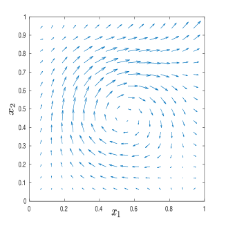
(a) Plot of $\bm{u}_{h}$ from (2.5)

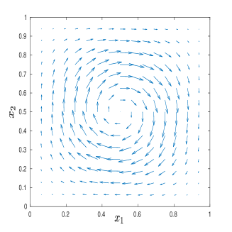
(b) Plot of $\bm{u}_{h}$ from (2.7)

Figure 1: Numerical velocity fields for (2.1) with $\nu=10^{-3}$ on a $16\times 16$ uniform triangulation of $\Omega=[0,1]^{2}$.

2.2 Convergence analysis

As we have pointed out earlier, the a priori error analysis of the stabilized $P_{1}\times P_{0}$ method (2.5) has not been established in the literature. In this subsection, we go one step further and present a new error estimate for the modified scheme (2.7) that is robust with respect to $\nu$, when $\nu\ll 1$. Our approach is to compare the error in the numerical approximation given by (2.7) with the error in the following scheme: Find $(\tilde{\bm{u}}_{h},\tilde{p}_{h})\in\bm{V}_{h}\times Q_{h}$ such that

$$\nu(\nabla\tilde{\bm{u}}_{h},\nabla\bm{v}_{h})-(\nabla\cdot\bm{v}_{h},\tilde{p}_{h}) =(\bm{f},\Pi_{h}\bm{v}_{h}), \quad\forall\bm{v}_{h}\in\bm{V}_{h},$$ (2.9)

$$(\nabla\cdot\tilde{\bm{u}}_{h},q_{h}) =0, \quad\forall q_{h}\in Q_{h}.$$

Following the analysis in [26], it is straightforward to show that

$$|\bm{u}-\tilde{\bm{u}}_{h}|_{1}\leq Ch|\bm{u}|_{2},$$ (2.10a)

$$\|p-\tilde{p}_{h}\|\leq Ch\big{(}\nu|\bm{u}|_{2}+|p|_{1}\big{)}.$$ (2.10b)

A local homogeneity argument implies

$$a_{h}^{b}(\bm{v}_{b},\bm{w}_{b})\simeq(\nabla\bm{v}_{b},\nabla\bm{w}_{b}),\quad\forall\bm{v}_{b},\bm{w}_{b}\in\bm{V}_{h}^{b},$$ (2.11)

i.e., $(\nabla\bullet,\nabla\bullet)|_{\bm{V}^{b}_{h}\times\bm{V}_{h}^{b}}$ is spectrally equivalent to $a_{h}^{b}.$ As a result, the modified bilinear form $a_{h}(\bullet,\bullet)$ is coercive

$$|\bm{v}|^{2}_{1,h}:=a_{h}(\bm{v}_{h},\bm{v}_{h})\simeq|\bm{v}_{h}|^{2}_{1},\quad\forall\bm{v}_{h}\in\bm{V}_{h}.$$ (2.12)

Let $\bm{V}_{h}^{\prime}$, $Q_{h}^{\prime}$ be the dual space of $\bm{V}_{h}$, $Q_{h}$, respectively. Given arbitrary functionals $\bm{F}\in\bm{V}^{\prime}_{h}$, $g\in Q^{\prime}_{h}$, we consider the following problem: Find $(\bm{v}^{F,g}_{h},q^{F,g}_{h})\in\bm{V}_{h}\times Q_{h}$ satisfying

$$\nu a_{h}(\bm{v}^{F,g}_{h},\bm{w}_{h})-(\nabla\cdot\bm{w}_{h},q^{F,g}_{h}) =\bm{F}(\bm{w}_{h}), \quad\forall\bm{w}_{h}\in\bm{V}_{h},$$

$$(\nabla\cdot\bm{v}^{F,g}_{h},r_{h}) =g(r_{h}), \quad\forall r_{h}\in Q_{h}.$$

Let $\bm{V}_{h}$ be equipped with the norm $\nu^{\frac{1}{2}}|\bullet|_{1}$ and $Q_{h}$ use the norm $\nu^{-\frac{1}{2}}\|\bullet\|$. Using the inf-sup condition (2.3), the coercivity of $a_{h}$, and the classical Babuška–Brezzi theory (cf. [7, 37]), we obtain the following stability estimate

$$\nu^{\frac{1}{2}}|\bm{v}^{F,g}_{h}|_{1,h}+\nu^{-\frac{1}{2}}\|q^{F,g}_{h}\|\leq\mathcal{K}\left(\beta^{-1}\right)\big{(}\sup_{\nu^{\frac{1}{2}}|\bm{w}_{h}|_{1}=1}\bm{F}(\bm{w}_{h})+\sup_{\nu^{-\frac{1}{2}}\|r_{h}\|=1}g(r_{h})\big{)},$$ (2.13)

where $\mathcal{K}$ is a fixed increasing function. Now we are in a position to present a robust error estimate of (2.7).

Theorem 2.1

For $(\bm{u}_{h},p_{h})$ given in (2.7), there exist absolute constants $C_{u}$, $C_{p}$ independent of $\nu$ and $h$, and such that

$$|\bm{u}-\bm{u}_{h}|_{1}\leq C_{u}h|\bm{u}|_{2},$$ (2.14a)

$$\|p-p_{h}\|\leq C_{p}h\big{(}\nu|\bm{u}|_{2}+|p|_{1}\big{)}.$$ (2.14b)

Proof 1

Consider the space of weakly divergence-free functions

$$\bm{W}_{h}:=\big{\{}\bm{v}_{h}\in\bm{V}_{h}:(\nabla\cdot\bm{v}_{h},q_{h})=0~{}\forall q_{h}\in Q_{h}\big{\}}.$$

By the definitions of $(\bm{u}_{h},p_{h})$ in (2.7) and $(\tilde{\bm{u}}_{h},\tilde{p}_{h})$ in (2.9), we have for all $\bm{v}\in\bm{V}_{h}$ and $q\in Q_{h}$:

$$a_{h}(\bm{u}_{h},\bm{v}_{h}) =(\nabla\tilde{\bm{u}}_{h},\nabla\bm{v}_{h})=0,\quad\forall\bm{v}_{h}\in\bm{W}_{h},$$ (2.15a)

$$\nu a_{h}(\bm{u}_{h},\bm{v}_{h})-(\nabla\cdot\bm{v}_{h},p_{h}) =\nu(\nabla\tilde{\bm{u}}_{h},\nabla\bm{v}_{h})-(\nabla\cdot\bm{v}_{h},\tilde{p}_{h}),\quad\forall\bm{v}_{h}\in\bm{V}_{h},$$ (2.15b)

$$(\nabla\cdot\bm{u}_{h},q_{h}) =(\nabla\cdot\tilde{\bm{u}}_{h},q_{h})=0,\quad\forall q_{h}\in Q_{h}.$$ (2.15c)

It then follows from (2.15a) and $a_{h}(\Pi_{h}\bm{u},\bm{v}_{h})=(\nabla\Pi_{h}\bm{u},\nabla\bm{v}_{h})$ that

$$a_{h}(\bm{u}_{h}-\Pi_{h}\bm{u},\bm{v}_{h})=\big{(}\nabla(\tilde{\bm{u}}_{h}-\Pi_{h}\bm{u}),\nabla\bm{v}_{h}\big{)},\quad\forall\bm{v}_{h}\in\bm{W}_{h}.$$ (2.16)

Combining (2.6) and $\nabla\cdot\bm{u}=0$, we conclude that $\nabla\cdot\Pi_{h}\bm{u}=0$ and thus $\Pi_{h}\bm{u}\in\bm{W}_{h}$. Therefore taking $\bm{v}_{h}=\bm{u}_{h}-\Pi_{h}\bm{u}\in\bm{W}_{h}$ in (2.16) and using (2.12) and the Cauchy–Schwarz inequality lead to

$$|\bm{u}_{h}-\Pi_{h}\bm{u}|^{2}_{1}\simeq a_{h}(\bm{v}_{h},\bm{v}_{h})\leq|\tilde{\bm{u}}_{h}-\Pi_{h}\bm{u}|_{1}|\bm{v}_{h}|_{1}.$$

As a consequence, it holds that

$$|\bm{u}_{h}-\Pi_{h}\bm{u}|_{1} \leq C|\tilde{\bm{u}}_{h}-\Pi_{h}\bm{u}|_{1}$$ (2.17)

$$\leq C|\bm{u}-\tilde{\bm{u}}_{h}|_{1}+C|\bm{u}-\Pi_{h}\bm{u}|_{1}.$$

Using (2.17) and a triangle inequality, we have

$$|\bm{u}-\bm{u}_{h}|_{1} \leq|\bm{u}-\Pi_{h}\bm{u}|_{1}+|\bm{u}_{h}-\Pi_{h}\bm{u}|_{1}$$ (2.18)

$$\leq C|\bm{u}-\Pi_{h}\bm{u}|_{1}+C|\bm{u}-\tilde{\bm{u}}_{h}|_{1}.$$

Combining (2.18) with (2.10a) and the interpolation error estimate of $\Pi_{h}$

$$|\bm{u}-\Pi_{h}\bm{u}|_{1}\leq Ch|\bm{u}|_{2}$$

finishes the proof of (2.14a).

Next, we pick arbitrary $\bm{w}_{l}\in\bm{V}_{h}^{l}$ and $r_{h}\in Q_{h}$ and use (2.15b), (2.15c) to obtain that

$$\nu a_{h}(\bm{u}_{h}-\bm{w}_{l},\bm{v}_{h})-(\nabla\cdot\bm{v}_{h},p_{h}-r_{h}) =\nu\big{(}\nabla(\tilde{\bm{u}}_{h}-\bm{w}_{l}),\nabla\bm{v}_{h}\big{)}-(\nabla\cdot\bm{v}_{h},\tilde{p}_{h}-r_{h}),\quad\forall\bm{v}_{h}\in\bm{V}_{h},$$ (2.19a)

$$(\nabla\cdot(\bm{u}_{h}-\bm{w}_{l}),q_{h}) =(\nabla\cdot(\tilde{\bm{u}}_{h}-\bm{w}_{l}),q_{h})=0,\quad\forall q_{h}\in Q_{h}.$$ (2.19b)

A combination of (2.19) and the stability estimate (2.13) then implies that for all $\bm{w}_{l}\in\bm{V}_{l}$, and $r_{h}\in Q_{h}$,

$$\nu^{\frac{1}{2}}|\bm{u}_{h}-\bm{w}_{l}|_{1,h}+\nu^{-\frac{1}{2}}\|p_{h}-r_{h}\| \leq\mathcal{K}(\beta^{-1})\big{(}\nu^{\frac{1}{2}}|\tilde{\bm{u}}_{h}-\bm{w}_{l}|_{1,h}+\nu^{-\frac{1}{2}}\|\tilde{p}_{h}-r_{h}\|\big{)}$$ (2.20)

$$\simeq\mathcal{K}(\beta^{-1})\big{(}\nu^{\frac{1}{2}}|\tilde{\bm{u}}_{h}-\bm{w}_{l}|_{1}+\nu^{-\frac{1}{2}}\|\tilde{p}_{h}-r_{h}\|\big{)}$$

$$\leq C\big{(}\nu^{\frac{1}{2}}|\bm{u}-\tilde{\bm{u}}_{h}|_{1}+\nu^{\frac{1}{2}}|\bm{u}-\bm{w}_{l}|_{1}+\nu^{-\frac{1}{2}}\|p-\tilde{p}_{h}\|+\nu^{-\frac{1}{2}}\|p-r_{h}\|\big{)}.$$

Using (2.20) and the triangle inequality, we have,

$$\|p-p_{h}\| \leq\|p-r_{h}\|+\|p_{h}-r_{h}\|$$

$$\leq C\big{(}\|p-r_{h}\|+\nu|\bm{u}-\tilde{\bm{u}}_{h}|_{1}+\nu|\bm{u}-\bm{w}_{l}|_{1}+\|p-\tilde{p}_{h}\|\big{)}.$$

Finally taking the infimum with respect to $(\bm{w}_{l},r_{h})\in\bm{V}_{h}^{l}\times Q_{h}$ in the above inequality and using (2.14a) concludes the proof of (2.14b).

3 Stationary Oseen equation

We now move on to the discretization of the stationary Navier–Stokes equation

$$-\nu\Delta\bm{u}+\bm{u}\cdot\nabla\bm{u}+\nabla p =\bm{f}\quad\text{ in }\Omega,$$ (3.1a)

$$\nabla\cdot\bm{u} =0\quad\text{ in }\Omega,$$ (3.1b)

$$\bm{u} =\bm{g}\quad\text{ on }\partial\Omega,$$ (3.1c)

with a potentially very small viscosity $\nu\ll 1$. As a first step, we consider the linear Oseen equation, which naturally occurs when (3.1) is linearized by a fixed point iteration:

$$-\nu\Delta\bm{u}+\bm{b}\cdot\nabla\bm{u}+\nabla p =\bm{f}\quad\text{ in }\Omega,$$ (3.2a)

$$\nabla\cdot\bm{u} =0\quad\text{ in }\Omega,$$ (3.2b)

$$\bm{u} =\bm{g}\quad\text{ on }\partial\Omega,$$ (3.2c)

Here, $\bm{b}:\Omega\rightarrow\mathbb{R}^{d}$ is a given convective field. For a reason which will become apparent later, we add a viscous term $-\varepsilon\Delta\bm{u}$ with vanishingly small $\varepsilon$, $0<\varepsilon\ll 1$ in (3.2a) and obtain the modified momentum equation

$$-\nu\Delta\bm{u}-\varepsilon\Delta\bm{u}+\bm{b}\cdot\nabla\bm{u}+\nabla p=\bm{f}.$$ (3.3)

Given a vector-valued $\bm{v}=(v_{1},\ldots,v_{d})^{\top}$, we consider the second order flux tensor

$$\mathbf{J}(\bm{v}):=\varepsilon\nabla\bm{v}+\bm{v}\otimes\bm{b}.$$ (3.4)

The $i$-th row of $\mathbf{J}(\bm{v})=(\bm{J}(v_{1})^{\top},\ldots,\bm{J}(v_{d})^{\top})^{\top}$ then is the standard flux

$$\bm{J}(v_{i}):=\varepsilon\nabla v_{i}+\bm{b}v_{i}$$

used in the classical EAFE discretization [36].

For each $E\in\mathcal{E}_{h},$ let $\bm{t}_{E}$ be a fixed unit vector tangent to the edge $E$, and let $\psi_{E}\in C^{1}(E)$ satisfy

$$\partial_{\bm{t}_{E}}\psi_{E}=\varepsilon^{-1}\bm{b}\cdot\bm{t}_{E},$$

where $\partial_{\bm{t}_{E}}$ is the directional derivative along $\bm{t}_{E}.$ We remark that $\psi_{E}$ is determined up to a constant. The following lemma could be found in [36].

Lemma 3.1

Let $\bm{\tau}_{E}=|E|\bm{t}_{E}$ be a non-unit vector tangent to $E\in\mathcal{E}_{h}$. We have

$$\delta_{E}(e^{\psi_{E}}v)=\fint_{E}\varepsilon^{-1}e^{\psi_{E}}\bm{J}(\bm{v})\cdot\bm{\tau}_{E}ds.$$ (3.5)

For a piecewise constant $\bm{J}_{h}$ vector field and a continuous and piecewise affine $w_{h}$ with respect to $\mathcal{T}_{h}$, we have

$$(\nabla w_{h},\bm{J}_{h})=-\sum_{E\in\mathcal{E}_{h}}a_{E}\delta_{E}w_{h}\bm{J}_{h}\cdot\bm{\tau}_{E},$$ (3.6)

where $\delta_{E}\chi=\chi(x_{j})-\chi(x_{i})$ with $E$ being the edge having endpoints $x_{i}$, $x_{j}$, $\bm{\tau}_{E}$ points from $x_{i}$ to $x_{j}$, and

$$a_{E}=a_{ij}:=\int_{\Omega}\nabla\lambda_{i}\cdot\nabla\lambda_{j}dx$$

is the $(i,j)$-entry of $P_{1}$ element stiffness matrix.

For $\bm{v}=(v_{1},\ldots,v_{d})^{\top}\in\bm{V}_{h}^{l}$, let $\mathbf{J}_{h}=(\bm{J}_{h}^{1\top},\ldots,\bm{J}_{h}^{d\top})^{\top}=P_{h}\mathbf{J}(\bm{v})$ be the piecewise constant $L^{2}$ projection of $\mathbf{J}(\bm{v})$ and thus $\bm{J}_{h}^{i}\approx\bm{J}(v_{i})$. It follows from (3.5) with $v=v_{i}$ that

$$\bm{J}_{h}^{i}\cdot\bm{\tau}_{E}\approx\varepsilon\left(\fint_{E}e^{\psi_{E}}ds\right)^{-1}\delta_{E}(e^{\psi_{E}}v_{i}).$$

Using this fact, integration by parts and (3.6), for a piecewise linear finite element approximation $\bm{u}_{h}^{l}=(\bm{u}_{h,1}^{l},\ldots,\bm{u}_{h,d}^{l})^{\top}$ to $\bm{u}$, we have

$$(-\varepsilon\Delta\bm{u}+\bm{b}\cdot\nabla\bm{u},\bm{v})=(\nabla\bm{u},\varepsilon\nabla\bm{v}+\bm{v}\otimes\bm{b})$$ (3.7)

$$=(\nabla\bm{u},\mathbf{J}(\bm{v}))\approx(\nabla\bm{u}_{h}^{l},\mathbf{J}_{h})=-\sum_{i=1}^{d}\sum_{E\in\mathcal{E}_{h}}a_{E}\delta_{E}u_{h,i}^{l}\bm{J}^{i}_{h}\cdot\bm{\tau}_{E}$$

$$\approx-\sum_{i=1}^{d}\sum_{E\in\mathcal{E}_{h}}\varepsilon a_{E}\left(\fint_{E}e^{\psi_{E}}ds\right)^{-1}\delta_{E}u_{h,i}^{l}\delta_{E}(e^{\psi_{E}}v_{i})$$

$$=-\sum_{E\in\mathcal{E}_{h}}\varepsilon a_{E}\left(\fint_{E}e^{\psi_{E}}ds\right)^{-1}\delta_{E}\bm{u}_{h}^{l}\cdot\delta_{E}(e^{\psi_{E}}\bm{v}).$$

As a consequence, we define the EAFE bilinear form $b^{\rm EAFE}_{h}:\bm{V}_{h}^{l}\times\bm{V}_{h}^{l}\rightarrow\mathbb{R}$ by

$$b^{\rm EAFE}_{h}(\bm{v}^{l}_{h},\bm{w}^{l}_{h};\bm{b}):=-\sum_{E\in\mathcal{E}_{h}}\varepsilon a_{E}\left(\fint_{E}e^{\psi_{E}}ds\right)^{-1}\delta_{E}\bm{v}^{l}_{h}\cdot\delta_{E}(e^{\psi_{E}}\bm{w}^{l}_{h}),\quad\forall\bm{v}_{h}^{l},\bm{w}_{h}^{l}\in\bm{V}_{h}^{l},$$

which is an variational form for discretizing $-\varepsilon\Delta\bm{u}+\bm{b}\cdot\nabla\bm{u}\approx\bm{b}\cdot\nabla\bm{u}$. We remark that the value of $b^{\rm EAFE}_{h}$ is not affected by the generic additive constant in $\psi_{E}$.

Remark 3.1

The original EAFE method [36] is designed for the convection-diffusion equation $-\nabla\cdot(\alpha\nabla u+\beta u)=f$ in conservative form. On the other hand, the EAFE bilinear form $b_{h}^{\rm EAFE}$ works for $-\nabla\cdot(\alpha\nabla u)+\beta\cdot\nabla u=f$ in convective form. In fact, $b_{h}^{\rm EAFE}$ depends on test functions weighted by edge-wise exponential functions while the classical EAFE scheme [36] makes use of an exponentially averaged trial function.

Using the modified equation (3.3), and the approximations $a(\bm{u},\bm{v}_{h})\approx a_{h}(\bm{u}_{h},\bm{v}_{h})$ and $(\bm{b}\cdot\nabla\bm{u},\bm{v}_{h}^{l})\approx b^{\rm EAFE}_{h}(\bm{u}_{h}^{l},\bm{v}^{l}_{h};\bm{b})$, we obtain a stabilized $P_{1}\times P_{0}$ EAFE scheme for the problem (3.2): Find $(\bm{u}_{h},p_{h})\in\bm{V}_{h}\times Q_{h}$ such that

$$\nu a_{h}(\bm{u}_{h},\bm{v}_{h})+b^{\rm EAFE}_{h}(\bm{u}^{l}_{h},\bm{v}^{l}_{h};\bm{b})-(\nabla\cdot\bm{v}_{h},p_{h}) =(\bm{f},\Pi_{h}\bm{v}_{h}), \quad\forall\bm{v}_{h}\in\bm{V}_{h},$$ (3.8)

$$(\nabla\cdot\bm{u}_{h},q_{h}) =0, \quad\forall q_{h}\in Q_{h}.$$

Here $b^{\rm EAFE}_{h}(\bm{v}_{h},\bm{w}_{h})$ is also defined for any continuous functions $\bm{v}_{h}$ and $\bm{w}_{h}$. However, it is easy to see that the value of $b^{\rm EAFE}_{h}$ is determined by nodal values of trial and test functions, i.e., $b^{\rm EAFE}_{h}(\bm{v}_{h},\bm{w}_{h};\bm{b})=b^{\rm EAFE}_{h}(\bm{v}^{l}_{h},\bm{w}^{l}_{h};\bm{b})$ for $\bm{v}_{h},\bm{w}_{h}\in\bm{V}_{h}$. Thus, the stabilizing face bubble functions in the BR element do not enter the discretized EAFE convective term.

Unfortunately, as numerical experiments show, the EAFE discretization given above for $\bm{b}\cdot\nabla\bm{u}$ does not work well. We now turn to the pressure-robust finite elements using discontinuous pressures [25, 26, 24]. Those works apply Raviart–Thomas or BDM interpolation to the test functions for the convective term $\bm{b}\cdot\nabla\bm{u}$. Similarly, we add a stabilization term with postprocessed bubble test functions to $b_{h}^{\rm EAFE}$ and obtain the following discrete convective form

$$b_{h}(\bm{v}_{h},\bm{w}_{h};\bm{b})=b_{h}(\bm{v}^{l}_{h},\bm{w}_{h};\bm{b})$$

$$\quad:=b_{h}^{\rm EAFE}(\bm{v}^{l}_{h},\bm{w}^{l}_{h};\bm{b})+(\bm{b}\cdot\nabla\bm{v}_{h}^{l},\Pi_{h}\bm{w}_{h}^{b}),\quad\forall\bm{v}_{h},\bm{w}_{h}\in\bm{V}_{h}.$$

The resulting scheme for (3.2) is: Find $(\bm{u}_{h},p_{h})\in\bm{Q}_{h}\times V_{h}$ such that

$$\nu a_{h}(\bm{u}_{h},\bm{v}_{h})+b_{h}(\bm{u}^{l}_{h},\bm{v}_{h};\bm{b})-(\nabla\cdot\bm{v}_{h},p_{h}) =(\bm{f},\Pi_{h}\bm{v}_{h}),\quad\forall\bm{v}_{h}\in\bm{V}_{h},$$ (3.9)

$$(\nabla\cdot\bm{u}_{h},q_{h}) =0,\quad\forall q_{h}\in Q_{h}.$$

In (3.9), let $\mathbf{A}_{bb}$, $\mathbf{A}_{ll}$, $\mathbf{A}_{bl}$, $\mathbf{A}_{lb}$, $\mathbf{A}_{bp}$, $\mathbf{A}_{lp}$ be the matrices representing the bilinear forms $\nu a_{h}(\bm{u}_{h}^{b},\bm{v}_{h}^{b})$, $\nu a_{h}(\bm{u}_{h}^{l},\bm{v}_{h}^{l})+b_{h}(\bm{u}_{h}^{l},\bm{v}_{h}^{l})$, $\nu a_{h}(\bm{u}_{h}^{l},\bm{v}_{h}^{b})+(\bm{b}\cdot\nabla\bm{u}_{h}^{l},\Pi_{h}\bm{v}_{h}^{b})$, $\nu a_{h}(\bm{u}_{h}^{b},\bm{v}_{h}^{l})$, $-(\nabla\cdot\bm{v}_{h}^{b},p_{h})$, $-(\nabla\cdot\bm{v}_{h}^{l},p_{h})$, respectively. Furthermore, let $\bm{U}_{b}$, $\bm{U}_{l}$, $\bm{P}$, $\bm{F}_{b}$, $\bm{F}_{l}$ be the vector representation for $\bm{u}_{h}^{b}$, $\bm{u}_{h}^{l}$, $p_{h}$, $(\bm{f},\Pi_{h}\bm{v}_{h}^{b})$ and $(\bm{f},\bm{v}_{h}^{l})$ (here $\Pi_{h}\bm{v}_{h}^{l}=\bm{v}_{h}^{l}$), respectively. The algebraic linear system for (3.9) then reads

$$\begin{pmatrix}\mathbf{A}_{bb}&\mathbf{A}_{bl}&\mathbf{A}_{bp}\\ \mathbf{A}_{lb}&\mathbf{A}_{ll}&\mathbf{A}_{lp}\\ \mathbf{A}_{bp}^{\top}&\mathbf{A}_{lp}^{\top}&\mathbf{O}\end{pmatrix}\begin{pmatrix}\bm{U}_{b}\\ \bm{U}_{l}\\ \bm{P}\end{pmatrix}=\begin{pmatrix}\bm{F}_{b}\\ \bm{F}_{l}\\ \bm{0}\end{pmatrix}.$$ (3.10)

Using the block Gaussian elimination, i.e. the static condensation, we obtain the reduced system

$$\begin{pmatrix}\mathbf{A}_{ll}-\mathbf{A}_{lb}\mathbf{A}^{-1}_{bb}\mathbf{A}_{bl}&\mathbf{A}_{lp}-\mathbf{A}_{lb}\mathbf{A}^{-1}_{bb}\mathbf{A}_{bp}\\ \mathbf{A}_{lp}^{\top}-\mathbf{A}_{bp}^{\top}\mathbf{A}^{-1}_{bb}\mathbf{A}_{bl}&-\mathbf{A}_{bp}^{\top}\mathbf{A}^{-1}_{bb}\mathbf{A}_{bp}\end{pmatrix}\begin{pmatrix}\bm{U}_{l}\\ \bm{P}\end{pmatrix}=\begin{pmatrix}\bm{F}_{l}-\mathbf{A}_{lb}\mathbf{A}_{bb}^{-1}\bm{F}_{b}\\ -\mathbf{A}_{bp}^{\top}\mathbf{A}^{-1}_{bb}\end{pmatrix}.$$ (3.11)

Let $N_{v}$ denote the number of interior vertices of $\mathcal{T}_{h}$, and $N_{t}$ the number of elements in $\mathcal{T}_{h}$. Since $\mathbf{A}_{bb}$ is a diagonal matrix, the stiffness matrix in (3.11) is sparse of dimension $(dN_{v}+N_{t})\times(dN_{v}+N_{t})$, the same as a $[P_{1}]^{d}\times P_{0}$ element. The vector $\bm{U}_{b}$ of dofs for the bubble component $\bm{u}^{b}_{h}$ are then recovered by $\bm{U}_{b}=\mathbf{A}_{bb}^{-1}(\bm{F}_{b}-\mathbf{A}_{bl}\bm{U}_{l}-\mathbf{A}_{bp}\bm{P})$.

Remark 3.2

We remark that the term $(\bm{b}\cdot\nabla\bm{u}_{h}^{b},\Pi_{h}\bm{v}_{h}^{b})$ is not added to (3.9). Otherwise the block $\mathbf{A}_{bb}$ is not diagonal and the above bubble reduction technique does not hold.

Let $b_{h,T}$ be the restriction of $b_{h}$ on $T\in\mathcal{T}_{h}$ and $E\in\mathcal{E}_{h}$ be an edge having endpoints $x_{i}$ and $x_{j}.$ When $\bm{b}$ is piecewise constant with respect to $\mathcal{T}_{h}$, the $(i,j)$-entry $b_{h,T}(\lambda_{j},\lambda_{i})$ of the local stiffness matrix for $b_{h,T}|_{\bm{V}_{h}^{l}\times\bm{V}_{h}^{l}}$ with $i\neq j$ is simple and written as

$$b_{h,T}(\lambda_{j},\lambda_{i})=\left\{\begin{aligned} &\varepsilon a_{ij}B(\varepsilon^{-1}\bm{b}|_{T}\cdot\bm{\tau}_{E}),\quad\bm{\tau}_{E}\text{ points from }x_{i}\text{ to }x_{j},\\ &\varepsilon a_{ij}B(-\varepsilon^{-1}\bm{b}|_{T}\cdot\bm{\tau}_{E}),\quad\bm{\tau}_{E}\text{ points from }x_{j}\text{ to }x_{i},\end{aligned}\right.$$ (3.12)

where $B$ is the Bernoulli function

$$B(s)=\left\{\begin{aligned} &\frac{s}{e^{s}-1},\quad&&s\neq 0,\\ &1,\quad&&s=0.\end{aligned}\right.$$ (3.13)

For $i=j$, we have $b_{h,T}(\lambda_{i},\lambda_{i})=-\sum_{j\neq i}b_{h,T}(\lambda_{i},\lambda_{j}).$ Therefore computing $b_{h}|_{\bm{V}_{h}^{l}\times\bm{V}_{h}^{l}}$ is no more complicated than assembling the stiffness matrix $(a_{ij})_{1\leq i,j\leq N}$ of the $P_{1}$ finite element method for Poisson’s equation.

(a) Plot of $|\bm{u}_{h}|$ from (3.9)

(b) Plot of $|\bm{u}_{h}|$ from (3.8)

Figure 2: Numerical speeds for (3.2) with $\nu=10^{-4}$, $\bm{b}=(10,1)^{\top}$ on a $16\times 16$ uniform triangulation of $\Omega=[0,1]^{2}$.

Now we compare the stabilized EAFE scheme (3.9) with the unstabilized one (3.8), where $\varepsilon=10^{-8}$. Consider the Oseen problem (3.2) with $\nu=10^{-4}$, $\bm{b}=(10,1)^{\top}$ and the exact solution

$$\bm{u}(\bm{x})=\big{(}\exp(x_{2}),\exp(x_{1})\big{)}^{\top},$$

$$p(\bm{x})=\exp(x_{1}+x_{2})-(\exp(1)-1)^{2}.$$

We set $\Omega=[0,1]\times[0,1]$ to be the unit square. The domain $\Omega$ is partitioned into a $16\times 16$ uniform grid of right triangles. Numerical solutions are visualized in Fig. 2. In this example, the speed profile from (3.9) is similar to the exponential exact speed $|\bm{u}|=\sqrt{\exp(2x_{1})+\exp(2x_{2})}$ while $|\bm{u}_{h}|$ from (3.8) exhibits an anomalous boundary layer.

Remark 3.3

For the convection-dominated elliptic problem $-\nabla\cdot(\alpha\nabla u+\bm{\beta}u)=f$, the classical EAFE scheme [36] makes use of $-\alpha\Delta u$ without adding an artificial viscous term $-\varepsilon\Delta u$. Similarly, for nearly inviscid incompressible flows (3.2) with $\nu\ll 1,$ it is tempting to use $-\nu\Delta\bm{u}$ instead of adding the vanishing viscosity term $-\varepsilon\Delta\bm{u}$ when deriving EAFE schemes (3.9), (4.1). However, an EAFE discretization for $-\nu\Delta\bm{u}+\bm{b}\cdot\nabla\bm{u}$ will not be Stokes stable because EAFE bilinear form does not take face bubbles into account.

Remark 3.4

The EAFE scheme (3.9) depends on the artificial diffusion constant $\varepsilon\ll 1.$ In practice, there is no need to tune this parameter once $\varepsilon$ is sufficiently small. For example, schemes using $\varepsilon=10^{-8}$ or $\varepsilon=10^{-10}$ have almost the same performance for benchmark problems.

4 Navier–Stokes equation

In view of the linear scheme (3.9), our method for the stationary Navier–Stokes equation (3.1) seeks $(\bm{u}_{h},p_{h})\in\bm{V}_{h}\times Q_{h}$ satisfying

$$\nu a_{h}(\bm{u}_{h},\bm{v}_{h})+b_{h}(\bm{u}^{l}_{h},\bm{v}_{h};P_{h}\bm{u}^{l}_{h})-(\nabla\cdot\bm{v}_{h},p_{h}) =(\bm{f},\Pi_{h}\bm{v}_{h}),\quad \forall~{}\bm{v}_{h}\in\bm{V}_{h},$$ (4.1)

$$(\nabla\cdot\bm{u}_{h},q_{h}) =0,\quad \forall~{}q_{h}\in Q_{h}.$$

We recall that $P_{h}\bm{u}^{l}_{h}$ is the element-wise average of the linear component $\bm{u}^{l}_{h}$ given by $P_{h}\bm{u}^{l}_{h}|_{T}=\frac{1}{|T|}\int_{T}\bm{u}^{l}_{h}dx$. In practice, we use the fixed-point iteration to solve (4.1) by iterating the third argument in $b_{h}.$ At each iteration step, the linearized finite element scheme reduces to (3.9). The assembling of stiffness matrices for linearized $b_{h}(\bullet,\bullet;P_{h}\bm{u}^{l}_{h})$ could be easily done using (3.12).

4.1 Time-dependent problems

In this subsection, we discuss the application of the stabilized $P_{1}\times P_{0}$ EAFE method to the original evolutionary Navier–Stokes equation (1.1). Applying the backward Euler method with time step-size $\tau>0$ to discretize $\bm{u}_{t}$ and (4.1) to spatial variables, we obtain the fully discrete scheme

$$(\bm{u}_{h,n},\bm{v}_{h})+\tau\nu a_{h}(\bm{u}_{h,n},\bm{v}_{h})+\tau b_{h}(\bm{u}^{l}_{h,n},\bm{v}_{h};P_{h}\bm{u}_{h,n}^{l})$$ (4.2)

$$\quad-\tau(\nabla\cdot\bm{v}_{h},p_{h,n})=\tau(\bm{f}(t_{n}),\Pi_{h}\bm{v}_{h})+(\bm{u}_{h,n-1},\bm{v}_{h}),$$

$$-\tau(\nabla\cdot\bm{u}^{n}_{h},q_{h})=0,$$

for all $(\bm{v}_{h},q_{h})\in\bm{V}_{h}\times Q_{h}$, where $t_{n}=n\tau$, $n=0,1,2,\ldots$, and $\bm{u}_{h,n}\approx\bm{u}(t_{n})$, $p_{h,n}\approx p(t_{n})$. However, the resulting algebraic system cannot be solved using the bubble reduction technique described in Section 3. The reason is that the term $(\bm{u}_{h,n}^{b},\bm{v}_{h}^{b})$ introduces an extra mass matrix and the block $\mathbf{A}_{bb}$ in (3.10) is no longer diagonal. To deal with such an issue, we consider the following quadrature on an element $T\in\mathcal{T}_{h}$:

$$\int_{T}fdx\approx\frac{|T|}{d+1}\sum_{F\in\mathcal{F},F\subset\partial T}f(\bm{x}_{F}),$$ (4.3)

where $\bm{x}_{F}$ is the barycenter of the face $F$. The formula (4.3) is second-order in $\mathbb{R}^{2}$ and first-order in $\mathbb{R}^{3}$. We then introduce a discrete $L^{2}$ vector inner product

$$(\bm{u},\bm{v})_{h}:=\frac{1}{d+1}\sum_{T\in\mathcal{T}_{h}}|T|\sum_{F\in\mathcal{F},F\subset\partial T}\bm{u}(x_{F})\cdot\bm{v}(x_{F}).$$ (4.4)

Replacing $(\bm{u}_{h,n},\bm{v}_{h}),(\bm{u}_{h,n-1},\bm{v}_{h})$ in (4.2) with $(\bm{u}_{h,n},\bm{v}_{h})_{h},(\bm{u}_{h,n-1},\bm{v}_{h})_{h}$, we arrive at the following modified time-dependent scheme: Find $\{\bm{u}_{h,n}\}_{n\geq 1}\subset\bm{V}_{h}$ and $\{p_{h,n}\}_{n\geq 1}\subset Q_{h}$ such that

$$(\bm{u}_{h,n},\bm{v}_{h})_{h}+\tau\nu a_{h}(\bm{u}_{h,n},\bm{v}_{h})+\tau b_{h}(\bm{u}^{l}_{h,n},\bm{v}_{h};P_{h}\bm{u}_{h,n}^{l})$$ (4.5)

$$\quad-\tau(\nabla\cdot\bm{v}_{h},p_{h,n})=\tau(\bm{f}(t_{n}),\Pi_{h}\bm{v}_{h})+(\bm{u}_{h,n-1},\bm{v}_{h})_{h}, \quad\forall\bm{v}_{h}\in\bm{V}_{h},$$

$$-\tau(\nabla\cdot\bm{u}_{h,n},q_{h})=0, \quad\forall q_{h}\in Q_{h}.$$

For two distinct faces $F\neq F^{\prime}\in\mathcal{F}_{h},$ it holds that

$$(\phi_{F}\bm{n}_{F},\phi_{F^{\prime}}\bm{n}_{F^{\prime}})_{h}=0.$$ (4.6)

Therefore the matrix representation for $(\bm{u}_{h,n}^{b},\bm{v}_{h}^{b})_{h}$ is a diagonal mass matrix and the linearized algebraic system for (4.5) in fixed point iterations is of the form (3.10), where $\mathbf{A}_{bb}$ is still a diagonal matrix corresponding to $(\bm{u}_{h,n}^{b},\bm{v}_{h}^{b})_{h}+\tau\nu a_{h}(\bm{u}_{h,n}^{b},\bm{v}_{h}^{b})$. As explained in (3.10), (3.11) in Section 3, the computational cost of solving (4.5) is comparable to a $[P_{1}]^{d}\times P_{0}$ element method.

Similarly to the stationary case, to enhance pressure-robustness, the work [24] replaces the terms $(\bm{u}_{h,n},\bm{v}_{h})$ and $(\bm{u}_{h,n-1},\bm{v}_{h})$ in a backward Euler method with $(\Pi_{h}\bm{u}_{h,n},\Pi_{h}\bm{v}_{h})$ and $(\Pi_{h}\bm{u}_{h,n-1},\Pi_{h}\bm{v}_{h})$, respectively. For our purpose, we can only postprocess the test function $\bm{v}_{h}$ as the term $(\Pi_{h}\bm{u}_{h,n}^{b},\Pi_{h}\bm{v}^{b}_{h})$ would contribute a non-diagonal mass matrix. The resulting time-dependent scheme is as follows: Find $\{\bm{u}_{h}^{n}\}_{n\geq 1}\subset\bm{V}_{h}$ and $\{p_{h}^{n}\}_{n\geq 1}\subset Q_{h}$ such that

$$(\bm{u}_{h,n},\Pi_{h}\bm{v}_{h})_{h}+\tau\nu a_{h}(\bm{u}_{h,n},\bm{v}_{h})+\tau b_{h}(\bm{u}^{l}_{h,n},\bm{v}_{h};P_{h}\bm{u}^{l}_{h,n})$$ (4.7)

$$\quad-\tau(\nabla\cdot\bm{v}_{h},p_{h,n})=\tau(\bm{f}(t_{n}),\Pi_{h}\bm{v}_{h})+(\bm{u}_{h,n-1},\Pi_{h}\bm{v}_{h})_{h}, \quad\forall\bm{v}_{h}\in\bm{V}_{h},$$

$$-\tau(\nabla\cdot\bm{u}_{h,n},q_{h})=0, \quad\forall q_{h}\in Q_{h}.$$

It follows from direct calculation and (2.8) that

$$(\phi_{F}\bm{n}_{F},\Pi_{h}(\phi_{F^{\prime}}\bm{n}_{F^{\prime}}))_{h}=c(\phi_{F}\bm{n}_{F},\bm{\phi}^{\rm RT}_{F^{\prime}})_{h}=0,\quad\forall F\neq F^{\prime}\in\mathcal{F}_{h},$$ (4.8)

where $c=|F|/6$ in $\mathbb{R}^{2}$ and $c=|F|/15$ in $\mathbb{R}^{3}$. Therefore the mass matrix from $(\bm{u}_{h,n}^{b},\Pi_{h}\bm{v}_{h}^{b})_{h}$ is diagonal and (4.7) could be solved in the same way as (4.5) and (4.1).

Remark 4.1

For Navier–Stokes equations with $\nu$ of moderate size, we could replace the EAFE form $b_{h}(\bm{u}_{h,n}^{l},\bm{v}_{h};P_{h}\bm{u}_{h,n}^{l})$ with $(\bm{u}_{h,n}\cdot\nabla\bm{u}^{l}_{h,n},\Pi_{h}\bm{v}_{h})$ and obtain a new stabilized $P_{1}\times P_{0}$ finite element method.

5 Numerical Experiments

In this section, we compare our schemes (3.9), (4.1), (4.5) with the standard BR finite element method using test functions postprocessed by the BDM interpolation $\Pi_{h}.$ Those postprocessing-based BR methods have been already argued in [26, 24, 23] to be superior to the classical ones. All experiments are performed in MATLAB R2020a and the linear solver is the MATLAB operation $\backslash$. For nonlinear problems, we use the fixed point iteration with 50 maximum number of iterations. The stopping criterion for nonlinear iterations is that the relative size of the increment $|\bm{X}_{k+1}-\bm{X}_{k}|/|\bm{X}_{k}|$ is below $10^{-6}$, where $\bm{X}_{k}$ is the solution for the linear system at the $k$-th iteration step. The parameter $\varepsilon$ used in our EAFE-based schemes is set to be $10^{-10}$.

5.1 Convection-dominated Oseen problem

First, we test the performance of (3.9) and the classical scheme (cf. [24, 23])

$$\nu(\nabla\bm{u}_{h},\nabla\bm{v}_{h})+(\bm{b}\cdot\nabla\bm{u}_{h},\Pi_{h}\bm{v}_{h})-(\nabla\cdot\bm{v}_{h},p_{h}) =(\bm{f},\Pi_{h}\bm{v}_{h}), \quad\forall\bm{v}_{h}\in\bm{V}_{h},$$ (5.1)

$$(\nabla\cdot\bm{u}_{h},q_{h}) =0, \quad\forall q_{h}\in Q_{h}$$

using the linear Oseen problem (3.2) with $\nu=10^{-3},$ $\bm{f}=10(-x_{2},x_{1})^{\top}$, $\bm{g}=(0,0)^{\top}$, $\bm{b}=(10,1)^{\top}$ on the unit square $\Omega=[0,1]\times[0,1]$. The mesh of $\Omega$ is relatively coarse and is shown in Fig. 3(a). We use the numerical velocity solution of (3.9) on a relatively fine uniform mesh with $51200$ triangles as the exact velocity field, see Fig. 3(b).

(a) The mesh used in Problem 5.1

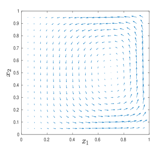
(b) The exact velocity field in Problem 5.1

Figure 3: The grid and exact velocity field for (3.2) used in Problem 5.1.

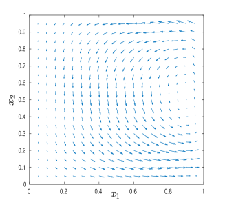
(a) Velocity field by the scheme (3.9)

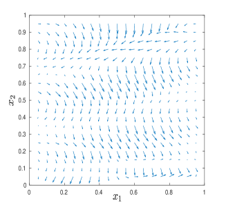
(b) Velocity field by the scheme (5.1)

Figure 4: Numerical velocity fields of the schemes (3.9) and (5.1) in Problem 5.1

Due to the sharp contrast between $\nu\ll|\bm{b}|$ and the homogeneous Dirichlet boundary condition, the exact velocity $\bm{u}$ is expected to have a sharp boundary layer. It could be observed from Fig. 4(b) that the classical scheme (5.1) yields a numerical velocity field with spurious oscillations in the low resolution setting. On the contrary, the stabilized EAFE scheme (3.9) is able to produce a physically meaningful solution Fig. 4(a) on a coarse mesh, compared with the reference velocity profile in Fig. 3(b).

5.2 Kovasznay flow

Table 1: Convergence history of the stabilized $P_{1}\times P_{0}$ EAFE scheme (4.1) in Problem 5.2

${\rm error}\backslash\#{\rm dof}$	225	961	3969	16129	65025	$\nu$
$\|\bm{u}-\bm{u}^{l}_{h}\|$	2.142	5.715e-1	1.448e-1	3.712e-2	9.976e-3	$1$
$\|p-p_{h}\|$	3.105e+1	1.995e+1	1.070e+1	5.465	2.746	$1$
$\|\bm{u}-\bm{u}^{l}_{h}\|$	3.557e-1	1.370e-1	4.039e-2	1.015e-2	3.309e-3	$10^{-3}$
$\|p-p_{h}\|$	2.151e-2	1.840e-2	1.048e-2	3.613e-3	1.567e-3	$10^{-3}$
$\|\bm{u}-\bm{u}^{l}_{h}\|$	3.560e-1	1.481e-1	4.496e-2	9.396e-3	2.516e-3	$5\times 10^{-4}$
$\|p-p_{h}\|$	1.317e-2	1.793e-2	1.041e-2	2.676e-3	8.949e-4	$5\times 10^{-4}$
$\|\bm{u}-\bm{u}^{l}_{h}\|$	3.589e-1	1.701e-1	9.665e-2	1.033e-2	2.180e-3	$10^{-4}$
$\|p-p_{h}\|$	1.258e-2	1.897e-2	1.905e-2	1.842e-3	4.462e-4	$10^{-4}$

Table 2: Convergence history of the classical scheme (5.2) in Problem 5.2

${\rm error}\backslash\#{\rm dof}$	401	1697	6977	28289	113921	$\nu$
$\|\bm{u}-\bm{u}^{l}_{h}\|$	1.922	4.436e-1	1.058e-1	2.584e-2	6.381e-3	$1$
$\|p-p_{h}\|$	2.886e+1	1.606e+1	8.293	4.183	2.095	$1$
$\|\bm{u}-\bm{u}^{l}_{h}\|$	1.057e+1	2.006e+1	4.569e-2	7.543e-3	1.668e-3	$10^{-3}$
$\|p-p_{h}\|$	4.178	3.125e+1	1.242e-2	1.868e-3	4.786e-4	$10^{-3}$
$\|\bm{u}-\bm{u}^{l}_{h}\|$	1.002e+1	9.190	9.815	9.131e-3	1.824e-3	$5\times 10^{-4}$
$\|p-p_{h}\|$	8.932	8.246e+1	5.006	2.277e-3	4.392e-4	$5\times 10^{-4}$
$\|\bm{u}-\bm{u}^{l}_{h}\|$	5.270	1.126e+1	1.651e+1	1.871e+1	5.078	$10^{-4}$
$\|p-p_{h}\|$	9.940	8.284	1.970e+1	4.239e+1	3.174	$10^{-4}$

For the stationary Navier–Stokes problem (3.1), we compare our scheme (3.9) with the following classical scheme (cf. [24, 23])

$$\nu(\nabla\bm{u}_{h},\nabla\bm{v}_{h})+(\bm{u}_{h}\cdot\nabla\bm{u}_{h},\Pi_{h}\bm{v}_{h})-(\nabla\cdot\bm{v}_{h},p_{h}) =(\bm{f},\Pi_{h}\bm{v}_{h}), \quad\forall\bm{v}_{h}\in\bm{V}_{h},$$ (5.2)

$$(\nabla\cdot\bm{u}_{h},q_{h}) =0, \quad\forall q_{h}\in Q_{h}$$

on the domain $\Omega=[-0.5,1.5]\times[0,2]$. The exact solution solutions of (3.1) are taken to be

$$\bm{u}(\bm{x})=\begin{pmatrix}1-e^{\lambda x_{1}}\cos(2\pi x_{2})\\ \frac{\lambda}{2\pi}e^{\lambda x_{1}}\sin(2\pi x_{2})\end{pmatrix},\quad p(\bm{x})=-\frac{1}{2}e^{2\lambda x_{1}}+\frac{1}{8\lambda}(e^{3\lambda}-e^{-\lambda}),$$ (5.3)

where $\lambda=\frac{1}{2\nu}-\sqrt{\frac{1}{4\nu^{2}}+4\pi^{2}}$ and $\nu$ is varying. In the literature, (5.3) is a benchmark problem known as the Kovasznay flow (cf. [15, 12, 11]). We start with a $8\times 8$ uniform initial partition of $\Omega$ having 128 triangles and then refine each element in the current mesh by quad-refinement to obtain finer grids. The data shown from 2nd to 6th columns in Tables 1 and 2 are computed on the same mesh. Since the bubble component of $\bm{u}_{h}$ has little effect on the accuracy, we only consider the approximation property of the linear part $\bm{u}_{h}^{l}$.

Without dofs associated with faces, the size of algebraic systems from (4.1) is significantly smaller than (5.2). In the case that $\nu=1$, the numerical accuracy of the classical scheme (5.2) is slightly better than the EAFE scheme (4.1). As $\nu$ is increasingly small, our EAFE-stabilized $P_{1}\times P_{0}$ method is able to yield numerical solutions with moderate accuracy even on the coarsest mesh. On the other hand, the performance of the classical method is not satisfactory on coarse meshes. In fact, the nonlinear iteration for (5.2) is not convergent unless the grid resolution is high enough.

5.3 Evolutionary potential flow

In the rest of two experiments, we investigate the effectiveness of (4.1) and (4.5) applied to benchmark potential flows proposed by Linke&Merdon [24]. Exact velocities of those problems are gradient of a harmonic polynomial. For potential flows, the pressure is relatively complicated and causes large velocity errors for numerical methods without pressure-robustness. Let $\chi(\bm{x},t)=t^{2}(5x_{1}^{4}x_{2}-10x_{1}^{2}x_{2}^{3}+x_{2}^{5})$ be a polynomial that is harmonic in space. We consider the evolutionary problem (1.1) with exact solutions

$$\bm{u}=\nabla\chi,\quad p=-\frac{|\bm{u}|^{2}}{2}-\chi_{t}+C,$$

where $C$ is a constant such that $\int_{\Omega}pdx=0.$ The corresponding load $\bm{f}=\bm{0}.$ The space domain $\Omega=[-0.5,0.5]\times[-0.5,0.5]$ and the time interval is $[0,2]$. We compare the EAFE $P_{1}\times P_{0}$ method (4.5) with the following classical scheme (cf. [24])

$$(\Pi_{h}\bm{u}_{h,n},\Pi_{h}\bm{v}_{h})+\tau\nu(\nabla\bm{u}_{h,n},\nabla\bm{v}_{h})+\tau b_{h}(\bm{u}_{h,n}\cdot\nabla\bm{u}_{h,n},\Pi_{h}\bm{v}_{h})$$ (5.4)

$$\quad-\tau(\nabla\cdot\bm{v}_{h},p_{h,n})=\tau(\bm{f}(t_{n}),\Pi_{h}\bm{v}_{h})+(\Pi_{h}\bm{u}_{h,n-1},\Pi_{h}\bm{v}_{h}),\quad \bm{v}_{h}\in\bm{V}_{h},$$

$$-\tau(\nabla\cdot\bm{u}_{h,n},q_{h})=0,\quad q_{h}\in Q_{h}.$$

We set the time step-size to be $\tau=0.1$ and use a uniform criss-cross mesh with 2048 right triangles.

For the potential flow with $\nu=1$, the numerical performance of the classical scheme (5.4) and the EAFE scheme (4.5) are comparable, see Table 3. When $\nu=10^{-6}$ is exceedingly small, it is observed from Table 4 that our stabilized $P_{1}\times P_{0}$ EAFE method outperforms the classical one. In particular, (5.4) stops converging after $t=1.5$ while our scheme (4.5) maintains moderate accuracy and outputs a relatively good solution at $t=2$, see Fig. 5.

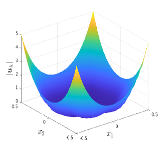
(a) Speed profile at $t=2$ by the scheme (4.5)

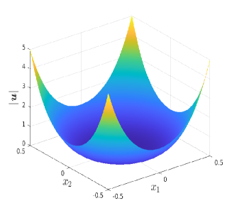
(b) Exact speed profile at $t=2$

Figure 5: Numerical and exact speed profiles in Problem 5.3, $t=2,$ $\nu=10^{-6}$

Table 3: A comparison between the schemes (4.5) and (5.4) in Problem 5.3, $\nu=1$.

$t$	$\|\bm{u}(t_{n})-\bm{u}^{l}_{h,n}\|$ in (4.5)	$\|p(t_{n})-p_{h,n}\|$ in (4.5)	$\|\bm{u}(t_{n})-\bm{u}^{l}_{h,n}\|$ in (5.4)	$\|p(t_{n})-p_{h,n}\|$ in (5.4)
$0.5$	4.640e-4	1.371e-2	3.890e-4	2.220e-2
$1.0$	1.855e-3	5.453e-2	1.556e-3	8.867e-2
$1.5$	4.164e-3	1.323e-1	3.501e-3	2.035e-1
$2.0$	7.387e-3	2.838e-1	6.224e-3	3.805e-1

Table 4: A comparison between the schemes (4.5) and (5.4) in Problem 5.3, $\nu=10^{-6}$.

$t$	$\|\bm{u}(t_{n})-\bm{u}^{l}_{h,n}\|$ in (4.5)	$\|p(t_{n})-p_{h,n}\|$ in (4.5)	$\|\bm{u}(t_{n})-\bm{u}^{l}_{h,n}\|$ in (5.4)	$\|p(t_{n})-p_{h,n}\|$ in (5.4)
$0.5$	2.893e-2	1.401e-2	1.962e-3	3.193e-3
$1.0$	8.857e-2	4.862e-2	3.548e-2	1.036e-2
$1.5$	1.420e-1	1.258e-1	2.014e+1	3.372e+2
$2.0$	1.946e-1	2.211e-1	1.085e+2	2.852e+3

5.4 3d potential flow

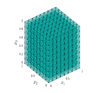
(a) The tetrahedral mesh in Problem 5.4

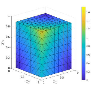
(b) Exact speed profile in Problem 5.4

Figure 6: The mesh and exact speed in Problem 5.4

(a) Speed profile by the scheme (4.1)

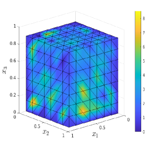
(b) Speed profile by the scheme (5.2)

Figure 7: Speed profiles of the schemes (4.1) and (5.2) when $\nu=10^{-4}$ in Problem 5.4

Table 5: A comparison between the schemes (4.1) and (5.2) in Problem 5.4

$\nu$	$\|\bm{u}-\bm{u}^{l}_{h}\|$ in (4.1)	$\|p-p_{h}\|$ in (4.1)	$\|\bm{u}-\bm{u}^{l}_{h}\|$ in (5.2)	$\|p-p_{h}\|$ in (5.2)
$1$	2.205e-3	4.393e-2	2.201e-3	4.037e-2
$10^{-1}$	2.234e-3	2.925e-2	2.220e-3	2.813e-2
$10^{-2}$	2.605e-3	2.872e-2	2.192e-3	2.799e-2
$10^{-3}$	4.639e-3	2.837e-2	2.192e-3	2.800e-2
$10^{-4}$	1.156e-2	2.804e-2	1.871	1.074e+1
$10^{-5}$	1.607e-2	2.806e-2	1.064e+1	2.454e+3

The last experiment is devoted to a 3 dimensional stationary Navier–Stokes problem (3.1) on the unit cube $\Omega=[0,1]\times[0,1]\times[0,1]$, where the exact solution is a steady-state potential flow

$$\bm{u}(\bm{x})=\nabla(x_{1}x_{2}x_{3}),\quad p=-\frac{1}{2}\nabla|\bm{u}|^{2}+C,$$ (5.5)

and $C$ is a constant such that $\int_{\Omega}pdx=0.$ The corresponding load $\bm{f}=\bm{0}.$ The mesh of $\Omega$ is a uniform tetrahedral grid with 3072 elements, see Fig. 6(a). Numerical results are presented in Fig. 7 and Table 5.

For viscosity $\nu$ of moderate size, the performance of (4.1) and (5.2) are similar while (4.1) solves more economic algebraic linear systems with much less number of dofs. When $\nu\leq 10^{-4}$, it is observed from Table 5 that the EAFE scheme (4.1) produces velocities and pressures of good quality on the fixed mesh while the fixed point iteration of (5.2) is indeed not convergent. Compared with (4.1), the classical scheme (5.2) produces highly oscillating solutions in the fixed point iteration when $\nu\leq 10^{-4}$, see the visualization of $|\bm{u}_{h}|$ at the cross sections $x_{1}=0.8$, $x_{2}=0.8$, $x_{3}=0.8$ in Fig. 7.

6 Concluding remarks

We have developed an EAFE-stabilized $P_{1}\times P_{0}$ finite element method for incompressible Navier–Stokes equations with small viscosity. For the Stokes problem, we have shown the robust a priori error analysis of our scheme with respect to $\nu$. It is straightforward to apply the technique in this paper to other Stokes element of the form $(P_{1}+{\it bubble})\times P_{0}$, see, e.g., the pointwise divergence-free Stokes elements in [20, 19]. Moreover, we shall investigate stabilized $P_{k}\times P_{k-1}$ schemes based on reducing higher order $(P_{k}+{\it bubble})\times P^{\rm disc}_{k-1}$ Stokes elements [18, 26, 20, 19] or other technique [16] and higher order EAFE [4, 34] in future research.

References

- [1] D. N. Arnold, F. Brezzi, and M. Fortin, A stable finite element for the Stokes equations, Calcolo 21 (1984), no. 4, 337–344 (1985). MR 799997
- [2] Ivo Babuška, The finite element method with Lagrangian multipliers, Numer. Math. 20 (1972/73), 179–192. MR 359352
- [3] Randolph E. Bank, W. M. Coughran Jr., and Lawrence C. Cowsar, The finite volume Scharfetter-Gummel method for steady convection diffusion equations, Comput. Visual Sci. 1 (1998), 123–136.
- [4] Randolph E. Bank, Panayot S. Vassilevski, and Ludmil T. Zikatanov, Arbitrary dimension convection-diffusion schemes for space-time discretizations, J. Comput. Appl. Math. 310 (2017), 19–31. MR 3544587
- [5] Christine Bernardi and Geneviève Raugel, Analysis of some finite elements for the Stokes problem, Math. Comp. 44 (1985), no. 169, 71–79. MR 771031
- [6] Daniele Boffi, Franco Brezzi, and Michel Fortin, Mixed finite element methods and applications, Springer Series in Computational Mathematics, vol. 44, Springer, Heidelberg, 2013. MR 3097958
- [7] Franco Brezzi, On the existence, uniqueness and approximation of saddle-point problems arising from Lagrangian multipliers, Rev. Française Automat. Informat. Recherche Opérationnelle Sér. Rouge 8 (1974), no. R-2, 129–151. MR 365287
- [8] Franco Brezzi, Jim Douglas Jr., and L. D. Marini, Two families of mixed finite elements for second order elliptic problems, Numer. Math. 2 (1985), no. 47, 217–235.
- [9] Alexander N. Brooks and Thomas J. R. Hughes, Streamline upwind/Petrov-Galerkin formulations for convection dominated flows with particular emphasis on the incompressible Navier-Stokes equations, Comput. Methods Appl. Mech. Engrg. 32 (1982), no. 1-3, 199–259, FENOMECH ”81, Part I (Stuttgart, 1981). MR 679322
- [10] Jesús Carrero, Bernardo Cockburn, and Dominik Schötzau, Hybridized globally divergence-free LDG methods. I. The Stokes problem, Math. Comp. 75 (2006), no. 254, 533–563. MR 2196980
- [11] Xi Chen and Yuwen Li, Superconvergent pseudostress-velocity finite element methods for the Oseen and Navier-Stokes equations, arXiv preprint (arXiv:2001.02805, 2021).
- [12] Xi Chen, Yuwen Li, Corina Drapaca, and John Cimbala, A unified framework of continuous and discontinuous Galerkin methods for solving the incompressible Navier-Stokes equation, J. Comp. Phys. 422 (2020), 109799.
- [13] , Some continuous and discontinuous Galerkin methods and structure preservation for incompressible flows, Internat. J. Numer. Methods Fluids 93 (2021), 2155–2174.
- [14] M. Crouzeix and P.-A. Raviart, Conforming and nonconforming finite element methods for solving the stationary Stokes equations, RAIRO Anal. Numér. 7 (1973), no. R-3, 33–75.
- [15] Daniele Antonio Di Pietro and Alexandre Ern, Mathematical aspects of discontinuous Galerkin methods, Mathématiques & Applications (Berlin) [Mathematics & Applications], vol. 69, Springer, Heidelberg, 2012. MR 2882148
- [16] Jim Douglas, Jr. and Jun Ping Wang, An absolutely stabilized finite element method for the Stokes problem, Math. Comp. 52 (1989), no. 186, 495–508. MR 958871
- [17] Leopoldo P. Franca and Thomas J. R. Hughes, Two classes of mixed finite element methods, Comput. Methods Appl. Mech. Engrg. 69 (1988), no. 1, 89–129. MR 953593
- [18] Vivette Girault and Pierre-Arnaud Raviart, Finite element methods for Navier-Stokes equations, Springer Series in Computational Mathematics, vol. 5, Springer-Verlag, Berlin, 1986, Theory and algorithms. MR 851383
- [19] Johnny Guzmán and Michael Neilan, Conforming and divergence-free Stokes elements in three dimensions, IMA J. Numer. Anal. 34 (2014), no. 4, 1489–1508. MR 3269433
- [20] , Conforming and divergence-free Stokes elements on general triangular meshes, Math. Comp. 83 (2014), no. 285, 15–36. MR 3120580
- [21] Johnny Guzmán, Chi-Wang Shu, and Filánder A. Sequeira, conforming and DG methods for incompressible Euler’s equations, IMA J. Numer. Anal. 37 (2017), no. 4, 1733–1771. MR 3712173
- [22] Thomas J. R. Hughes, Leopoldo P. Franca, and Marc Balestra, A new finite element formulation for computational fluid dynamics. V. Circumventing the Babuška-Brezzi condition: a stable Petrov-Galerkin formulation of the Stokes problem accommodating equal-order interpolations, Comput. Methods Appl. Mech. Engrg. 59 (1986), no. 1, 85–99. MR 868143
- [23] Volker John, Alexander Linke, Christian Merdon, Michael Neilan, and Leo G. Rebholz, On the divergence constraint in mixed finite element methods for incompressible flows, SIAM Rev. 59 (2017), no. 3, 492–544. MR 3683678
- [24] A. Linke and C. Merdon, Pressure-robustness and discrete Helmholtz projectors in mixed finite element methods for the incompressible Navier-Stokes equations, Comput. Methods Appl. Mech. Engrg. 311 (2016), 304–326. MR 3564690
- [25] Alexander Linke, On the role of the Helmholtz decomposition in mixed methods for incompressible flows and a new variational crime, Comput. Methods Appl. Mech. Engrg. 268 (2014), 782–800. MR 3133522
- [26] Alexander Linke, Gunar Matthies, and Lutz Tobiska, Robust arbitrary order mixed finite element methods for the incompressible Stokes equations with pressure independent velocity errors, ESAIM Math. Model. Numer. Anal. 50 (2016), no. 1, 289–309. MR 3460110
- [27] Maxim A. Olshanskii, A low order Galerkin finite element method for the Navier-Stokes equations of steady incompressible flow: a stabilization issue and iterative methods, Comput. Methods Appl. Mech. Engrg. 191 (2002), no. 47-48, 5515–5536. MR 1941488
- [28] Maxim A. Olshanskii and Arnold Reusken, Grad-div stabilization for Stokes equations, Math. Comp. 73 (2004), no. 248, 1699–1718. MR 2059732
- [29] P.-A. Raviart and J. M. Thomas, A mixed finite element method for 2nd order elliptic problems, Mathematical aspects of finite element methods (Rome), (Proc. Conf., Consiglio Naz. delle Ricerche (C.N.R.), 1977, pp. 292–315. Lecture Notes in Math., Vol. 606. MR 0483555
- [30] C. Rodrigo, X. Hu, P. Ohm, J. H. Adler, F. J. Gaspar, and L. T. Zikatanov, New stabilized discretizations for poroelasticity and the Stokes’ equations, Comput. Methods Appl. Mech. Engrg. 341 (2018), 467–484. MR 3845633
- [31] D. L. Scharfetter and H. K. Gummel, Large-signal analysis of a silicon read diode oscillator, IEEE Transactions on Electron Devices 16 (1969), no. 267, 64–77.
- [32] L. R. Scott and M. Vogelius, Conforming finite element methods for incompressible and nearly incompressible continua, Large-scale computations in fluid mechanics, Part 2 (La Jolla, Calif., 1983), Lectures in Appl. Math., vol. 22, Amer. Math. Soc., Providence, RI, 1985, pp. 221–244. MR 818790
- [33] Shuonan Wu and Jinchao Xu, Simplex-averaged finite element methods for , , and convection-diffusion problems, SIAM J. Numer. Anal. 58 (2020), no. 1, 884–906. MR 4069328
- [34] Shuonan Wu and Ludmil T. Zikatanov, On the unisolvence for the quasi-polynomial spaces of differential forms, 2020, arXiv 2003.14278 (math.NA).
- [35] Jin-chao Xu and Lung-an Ying, Convergence of an explicit upwind finite element method to multi-dimensional conservation laws, J. Comput. Math. 19 (2001), no. 1, 87–100. MR 1807107
- [36] Jinchao Xu and Ludmil Zikatanov, A monotone finite element scheme for convection-diffusion equations, Math. Comp. 68 (1999), no. 228, 1429–1446. MR 1654022
- [37] , Some observations on Babuška and Brezzi theories, Numer. Math. 94 (2003), no. 1, 195–202. MR 1971217
- [38] Shangyou Zhang, A new family of stable mixed finite elements for the 3D Stokes equations, Math. Comp. 74 (2005), no. 250, 543–554. MR 2114637