Popularity Adjusted Block Models are Generalized Random Dot Product Graphs

Abstract

We connect two random graph models, the Popularity Adjusted Block Model (PABM) and the Generalized Random Dot Product Graph (GRDPG), by demonstrating that the PABM is a special case of the GRDPG in which communities correspond to mutually orthogonal subspaces of latent vectors. This insight allows us to construct new algorithms for community detection and parameter estimation for the PABM, as well as improve an existing algorithm that relies on Sparse Subspace Clustering. Using established asymptotic properties of Adjacency Spectral Embedding for the GRDPG, we derive asymptotic properties of these algorithms. In particular, we demonstrate that the absolute number of community detection errors tends to zero as the number of graph vertices tends to infinity. Simulation experiments illustrate these properties.

Keywords: network analysis, block models, generalized random dot product graphs, community detection, sparse subspace clustering

1 Introduction

Statistical inference on random graphs requires a suitable probability model. A general probability model for unweighted and undirected graphs is the Bernoulli Graph (also known as the inhomogeneous Erdös-Rényi model), which assumes that edges occur as independent Bernoulli trials. A Bernoulli Graph is characterized by an edge probability matrix $P=[P_{ij}]$, where an edge between vertices $i$ and $j$ occurs with success probability $P_{ij}$. A trivial example of a Bernoulli Graph is the (homogeneous) Erdös-Rényi model proposed by [7], in which the vertices of the random graph are fixed and possible edges occur independently with fixed probability $P_{ij}=p$ for all $i,j$. The requirement that $P_{ij}\equiv p$ for all $i,j$ is too strong for most applications, and various researchers have weakened that requirement in various ways. The present work relates two lines of generalization.

Network analysis is often concerned with community detection. One form of community detection assumes that each vertex belongs to an unobserved community, with the probability of an edge between vertices $i$ and $j$ depending on the communities to which $i$ and $j$ belong. Formally, one assigns each vertex $v_{i}$ a community label $z_{i}$ and assumes a Bernoulli Graph in which $P_{ij}$ is a function of $z_{i}$ and $z_{j}$. Such models, called Block Models, define the goal of community detection as a problem in statistical inference: identify the true community (up to permutation of labels) to which each vertex belongs.

The classical Stochastic Block Model (SBM) of [13] specifies that each edge probability $P_{ij}$ depends only on the labels $z_{i}$ and $z_{j}$, i.e., $P_{ij}=\omega_{z_{i},z_{j}}$. Subsequent researchers have weakened this assumption. The Degree-Corrected Block Model (DCBM) of [10] assigns an additional parameter $\theta_{i}$ to each vertex and sets $P_{ij}=\theta_{i}\theta_{j}\omega_{z_{i},z_{j}}$. The Popularity Adjusted Block Model (PABM) of [17] generalizes the DCBM, allowing heterogeneity of edge probabilities within and between communities while still maintaining distinct community structure.

Another type of Bernoulli Graph was proposed by [22]. A Random Dot Product Graph (RDPG) specifies that each vertex corresponds to a latent position vector in Euclidean space and that the probability of an edge between two vertices is the dot product of their latent position vectors. Thus, if the latent positions are $x_{1},\ldots,x_{n}\in\mathbb{R}^{d}$ and $X=\bigl{[}x_{1}\mid\dots\mid x_{n}\bigr{]}^{\top}$, then the edge probability matrix is $P=XX^{\top}$. Clearly, any Bernoulli Graph with positive semidefinite $P$ is an RDPG. The positive definite Euclidean inner product in the RDPG model was replaced by an indefinite inner product in [16], resulting in the Generalized RDPG (GRDPG).

In contrast to Block Models, neither RDPGs nor GRDPGs inherently specify distinct communities. However, one can easily impose community structure by assuming that the latent positions lie in distinct clusters. Hence, it is not surprising that Block Models can be studied by reformulating them as RDPGs or GRDPGs. For example, an assortative SBM (an SBM for which $P$ is positive semidefinite) is equivalent to an RDPG for which all vertices in the same community correspond to the same latent position vector. Likewise, the DCBM is equivalent to an RDPG for which all vertices in the same community correspond to latent position vectors that lie on a straight line.

Because the edge probability matrix of a PABM is not necessarily positive semidefinite, a PABM is not necessarily an RDPG. In Section 2.3 we demonstrate that every PABM is in fact a specific type of GRDPG for which the latent position vectors lie in distinct orthogonal subspaces, each subspace corresponding to a community. This identification is our central result. In Section 3, we use the geometry of the GRDPG to derive more efficient algorithms for detecting the communities and estimating the parameters in the PABM. We report the results of simulation studies in Section 4 and apply our methods to three well-known data sets in Section 5. Section 6 concludes. Proofs of Theorems 1 and 2 are provided in the body of the text while proofs of Theorems 3, 4, and 5 are provided in the Appendix.

2 PABMs are GRDPGs

In this section, we show that the PABM is a special case of the GRDPG. More specifically, a graph $G$ drawn from the PABM can be represented by a collection of latent vectors in Euclidean space. We further show that the latent configuration that induces the PABM consists of orthogonal subspaces with each subspace corresponding to a community.

2.1 Notation and Scope

Let $G=(V,E)$ be an unweighted, undirected graph without self-loops, with vertex set $V$ ($|V|=n$) and edge set $E$. The matrix $A\in\{0,1\}^{n\times n}$ represents the adjacency matrix of $G$ such that $A_{ij}=1$ if there exists an edge between vertices $i$ and $j$ and $0$ otherwise. $A_{ij}=A_{ji}$ and $A_{ii}=0$ for each $i,j\in[n]$ (where $[n]=\{1,2,...,n\}$). We further restrict our analyses to Bernoulli graphs. Let $P\in[0,1]^{n\times n}$ be a symmetric matrix of edge probabilities. Graph $G$ is sampled from $P$ by drawing $A_{ij}\stackrel{{\scriptstyle\mathrm{ind}}}{{\sim}}\mathrm{Bernoulli}(P_{ij})$ for each $1\leq i<j\leq n$ (setting $A_{ji}=A_{ij}$ and $A_{ii}=0$). We denote $A\sim\mathrm{BernoulliGraph}(P)$ as a graph with adjacency matrix $A$ sampled from edge probability matrix $P$ in this manner. If each vertex has a hidden label in $[K]$, they are denoted as $z_{1},...,z_{n}$. $\lambda_{ik}$ denotes the popularity parameter of vertex $i$ to community $k$. $\Lambda$ is the $n\times K$ matrix of popularity parameters. Finally, we denote $X=\bigl{[}x_{1}\mid\cdots\mid x_{n}\bigr{]}^{\top}\in\mathbb{R}^{n\times d}$ as the matrix corresponding to a collection of $n$ latent vectors $x_{1},...,x_{n}\in\mathbb{R}^{d}$.

2.2 Two Probability Models for Graphs

Definition 1 (Popularity Adjusted Block Model).

Let $K\geq 1$ be an integer and let $\Lambda\in\mathbb{R}^{n\times K}$ be a matrix with entries in $[0,1]$. Let $z_{1},z_{2},\dots,z_{n}\in[K]$. A graph $G$ with adjacency matrix $A$ is said to be a popularity adjusted block model graph with $K$ communities, popularity vectors $\Lambda$, and sparsity parameter $\rho_{n}\in(0,1]$ if $A\sim\mathrm{BernoulliGraph}(P)$ where the edge probability matrix $P$ has entries $P_{ij}$, $i,j\in[n]$, of the form

$$P_{ij}=\rho_{n}\lambda_{iz_{j}}\lambda_{jz_{i}}.$$

Remark 1.

In a PABM, each vertex $i$ has $K$ popularity parameters $\lambda_{i1},\dots,\lambda_{iK}$, that describe its affinity toward each of the $K$ communities. Another view of a PABM is as follows. Let $\tilde{P}$ be the matrix obtained by permuting the rows and columns of $P$ so that the vertices are reorganized by community memberships $z_{i}\in\{1,2,\dots,K\}$ in increasing order. Denote by $\tilde{P}^{(k\ell)}$ the $n_{k}\times n_{\ell}$ submatrix of $\tilde{P}$ corresponding to the edge probabilities between vertices in communities $k$ and $\ell$. Here $n_{k}=|\{i\colon z_{i}=k\}|$ is the number of vertices assigned to community $k$, for $k=1,2\dots,K$. Note that $\tilde{P}^{(k\ell)}=(\tilde{P}^{(\ell k)})^{\top}$. Next let $\lambda^{(k\ell)}=\{\lambda_{i\ell}\colon z_{i}=k\}\in\mathbb{R}^{n_{k}}$; the elements of $\lambda^{(k\ell)}$ are the affinity parameters toward the $\ell$th community of all vertices in the $k^{th}$ community. Define $\lambda^{(\ell k)}$ analogously. Then each block $\tilde{P}^{(k\ell)}$ can be written as the outer product of two vectors:

$$\tilde{P}^{(k\ell)}=\rho_{n}\lambda^{(k\ell)}(\lambda^{(\ell k)})^{\top}.$$ (1)

We will henceforth use the notation $A\sim\mathrm{PABM}(\{\lambda^{(k\ell)}\}_{K},\rho_{n})$ to denote a random adjacency matrix $A$ drawn from a PABM with $K$ communities, popularity parameters $\{\lambda^{(k\ell)}\}$ and sparsity parameter $\rho_{n}$.

The sparsity parameter $\rho_{n}$ in the definition of the PABM influences the degrees of the vertices in the sampled graphs $A\sim\mathrm{BernoulliGraph}(P)$. In particular, for a fixed $\Lambda$, the graphs become sparser as $\rho_{n}$ decreases. Note that $\rho_{n}$ and $\Lambda$ are not uniquely identifiable, i.e., we can scale $\rho_{n}$ by a constant $c>0$ and scale $\Lambda$ by $c^{-1/2}$ without changing the edge probabilities in $P$. Thus, for ease of exposition, we shall assume henceforth that (1) $\Lambda$ is normalized to have Frobenius norm $\|\Lambda\|_{F}=\sqrt{n}$ and (2) the $\ell_{2}$ norms of the rows of $\|\Lambda\|$ are all bounded away from $0$. Under these two assumptions, the sparsity parameter $\rho_{n}$ can now be viewed as controlling the density of $A$, i.e., the average degree of $A$ grows at rate $n\rho_{n}$ and the number of edges grows at rate $n^{2}\rho_{n}$. The choice $\rho_{n}\equiv 1$ and $\rho_{n}\rightarrow 0$ then corresponds to the dense graphs regime and semi-sparse graphs regime, respectively.

Definition 2 (Generalized Random Dot Product Graph).

Let $p\geq 1$ and $q\geq 0$ be integers. Define $I_{p,q}$ as the block diagonal matrix $I_{p,q}=\Bigl{[}\begin{smallmatrix}I_{p}&0\\ 0&-I_{q}\end{smallmatrix}\Bigr{]}$ where $I_{p}$ and $I_{q}$ are the identity matrices of dimensions $p\times p$ and $q\times q$ respectively. Denote $d=p+q$ and let $\mathcal{X}$ be a subset of $\mathbb{R}^{d}$ such that, for any $x\in\mathcal{X}$ and $y\in\mathcal{X}$, we have $x^{\top}I_{p,q}y\in[0,1]$. Let $X=\bigl{[}x_{1}\mid\cdots\mid x_{n}\bigr{]}^{\top}$ be a $n\times d$ matrix with rows $x_{i}\in\mathcal{X}$. A graph $G$ with adjacency matrix $A$ is said to be a generalized random dot product graph with latent positions $X$, sparsity parameter $\rho_{n}\in(0,1]$ and signature $(p,q)$ if $A\sim\mathrm{BernoulliGraph}(P)$ where the edge probability matrix $P$ is given by $P=\rho_{n}XI_{p,q}X^{\top}$, i.e., the entries of $P$ are of the form $P_{ij}=\rho_{n}x_{i}^{\top}I_{p,q}x_{j}.$

We will use the notation $A\sim\mathrm{GRDPG}_{p,q}(X;\rho_{n})$ to denote a random adjacency matrix $A$ drawn from latent positions $X$, sparsity parameter $\rho_{n}$ and signature $(p,q)$.

Definition 3 (Indefinite Orthogonal Group).

The indefinite orthogonal group with signature $(p,q)$ is the set $\{Q\in\mathbb{R}^{d\times d}\colon QI_{p,q}Q^{\top}=I_{p,q}\}$, denoted as $\mathbb{O}(p,q)$. Here $d=p+q$.

Remark 2.

The latent vectors that produce $XI_{p,q}X^{\top}=P$ are not unique [16]. More specifically, if $P_{ij}=x_{i}^{\top}I_{p,q}x_{j}$, then for any $Q\in\mathbb{O}(p,q)$ we also have $(Qx_{i})^{\top}I_{p,q}(Qx_{j})=x_{i}^{\top}(Q^{\top}I_{p,q}Q)x_{j}=x_{i}^{\top}I_{p,q}x_{j}=P_{ij}$. Unlike in the RDPG case, transforming the latent positions via multiplication by $Q\in\mathbb{O}(p,q)$ does not necessarily maintain interpoint angles or distances.

Remark 3.

We can use Adjacency Spectral Embedding (ASE) [19] to recover the latent vectors of a GRDPG. This procedure consists of taking the spectral decomposition of $A$ and keeping the $p+q$ largest eigenvalues (in modulus) and corresponding eigenvectors of $A$. More specifically, let $A$ be an $n\times n$ adjacency matrix and denote the eigendecomposition of $A$ as

$$A=\sum_{i}\hat{\lambda}_{i}\hat{v}_{i}\hat{v}_{i}^{\top},\quad\text{where}\,\,|\hat{\lambda}|_{1}\geq|\hat{\lambda}_{2}|\geq\dots\geq|\hat{\lambda}_{n}|.$$

Let $\hat{D}$ be a diagonal matrix whose diagonal entries are the eigenvalues $\{\hat{\lambda}_{i}\}_{i=1}^{d}$ arranged in decreasing values (not in decreasing modulus) and let $\hat{V}$ be the $n\times d$ matrix whose columns are the corresponding eigenvectors $\{\hat{v}_{i}\}_{i=1}^{d}$ arranged in the same order as the diagonal entries of $\hat{D}$. Now define $\hat{Z}=\hat{V}|\hat{D}|^{1/2}$ where the $|\cdot|$ operation is applied elementwise to the entries of $\hat{D}$. Then $\hat{Z}$ serves as an estimate of $X$, up to some non-identifiable orthogonal transformation $Q$ as described in Remark 2 and Definition 3; see [16] for further details.

2.3 The Geometry of PABMs

Now that we defined the PABM and GRDPG, we show the special geometry of the PABM when viewed as a GRDPG. For ease of exposition, and without loss of generality, we drop the dependency on the sparsity parameter $\rho_{n}$ and assume $\rho_{n}\equiv 1$ throughout this subsection.

Theorem 1 (The latent configuration of the PABM).

Let $A\sim\mathrm{PABM}(\{\lambda^{(k\ell)}\}_{K})$ be an instance of a PABM with $K\geq 1$ blocks and latent vectors $\{\lambda^{(k\ell)}\colon 1\leq k\leq K,1\leq\ell\leq K\}$. Then there exists a block diagonal matrix $X\in\mathbb{R}^{n\times K^{2}}$ defined by $\{\lambda^{(k\ell)}\}$ and a $K^{2}\times K^{2}$ fixed orthonormal matrix $U$ such that $A\sim\mathrm{GRDPG}_{K(K+1)/2,K(K-1)/2}(\tilde{\Pi}XU)$. Here $\tilde{\Pi}$ is the permutation matrix such that $P=\tilde{\Pi}\tilde{P}\tilde{\Pi}^{\top}$ where the rows and columns of $\tilde{P}$ are arranged according to increasing values of the community labels (see Remark 1).

Proof.

We will prove this theorem in two parts. First, for demonstration purposes, we focus on the case when $K=2$ to build intuition. The general case of $K\geq 2$ is presented later.

For the $K=2$ case, the proof is straightforward. We will first work with the matrix $\tilde{P}$. Note that $\tilde{P}$ has the form

$$\tilde{P}=\begin{bmatrix}P^{(11)}&P^{(12)}\\ P^{(21)}&P^{(22)}\end{bmatrix}=\begin{bmatrix}\lambda^{(11)}(\lambda^{(11)})^{\top}&\lambda^{(12)}(\lambda^{(21)})^{\top}\\ \lambda^{(21)}(\lambda^{(12)})^{\top}&\lambda^{(22)}(\lambda^{(22)})^{\top}\end{bmatrix}.$$

Now let

$$X=\begin{bmatrix}\lambda^{(11)}&\lambda^{(12)}&0&0\\ 0&0&\lambda^{(21)}&\lambda^{(22)}\end{bmatrix}\quad\text{and}\quad U=\begin{bmatrix}1&0&0&0\\ 0&0&1/\sqrt{2}&1/\sqrt{2}\\ 0&0&1/\sqrt{2}&-1/\sqrt{2}\\ 0&1&0&0\end{bmatrix}.$$

Then by straightforward matrix multiplication, we obtain

$$XUI_{3,1}U^{\top}X^{\top}=\begin{bmatrix}\lambda^{(11)}(\lambda^{(11)})^{\top}&\lambda^{(12)}(\lambda^{(21)})^{\top}\\ \lambda^{(21)}(\lambda^{(12)})^{\top}&\lambda^{(22)}(\lambda^{(22)})^{\top}\end{bmatrix}=\tilde{P}$$

and hence $\tilde{P}$ also corresponds to the edge probability matrix of GRDPG with latent vectors described by $XU$. As $P=\tilde{\Pi}\tilde{P}\tilde{\Pi}^{\top}$ we conclude that $P$ has latent vectors described by $\tilde{\Pi}XU$.

It is nevertheless instructive to look at a few intermediate steps. More specifically, the product $UI_{3,1}U^{\top}$ yields a permutation matrix $\Pi$ with fixed points at positions $1$ and $4$ and a cycle of order 2 swapping positions $2$ and $3$, i.e.,

$$\Pi=UI_{3,1}U^{\top}=\begin{bmatrix}1&0&0&0\\ 0&0&1&0\\ 0&1&0&0\\ 0&0&0&1\end{bmatrix}.$$

Furthermore, as $U$ is orthonormal and $I_{3,1}$ is diagonal, $UI_{3,1}U^{\top}$ is also an eigendecomposition of $\Pi$ where the fixed points of $\Pi$ are mapped to the eigenvectors $e_{1}$ and $e_{4}$ while the cycles of order two are mapped to the eigenvectors $\tfrac{1}{\sqrt{2}}(e_{2}+e_{3})$ and $\tfrac{1}{\sqrt{2}}(e_{2}-e_{3})$; here $e_{i}$ denote the $i^{\mathrm{th}}$ basis vector in $\mathbb{R}^{4}$. Thus, another way of decomposing the edge probability matrix is $\tilde{P}=X\Pi X^{\top}$ where the rows of $X$ lie in the union of two 2-dimensional orthogonal subspaces and $\Pi$ is a permutation matrix.

For the general case, we can extend $\tilde{P}=X\Pi X^{\top}$ to larger $K$. For a more concrete example of this, refer to Example 1. We once again consider $\tilde{P}$ as defined in Remark 1. We first define the following matrices

$$\Lambda^{(k)}=\begin{bmatrix}\lambda^{(k1)}\mid\cdots\mid\lambda^{(kK)}\end{bmatrix}\in\mathbb{R}^{n_{k}\times K},\quad X=\mathrm{blockdiag}(\Lambda^{(1)},\dots,\Lambda^{(K)})\in\mathbb{R}^{n\times K^{2}},$$ (2)

$$L^{(k)}=\mathrm{blockdiag}(\lambda^{(1k)},\dots,\lambda^{(Kk)})\in\mathbb{R}^{n\times K},\quad Y=\begin{bmatrix}L^{(1)}\mid\cdots\mid L^{(K)}\end{bmatrix}\in\mathbb{R}^{n\times K^{2}}.$$ (3)

It is then straightforward to verify that

$$XY^{\top}=\mathrm{blockdiag}(\Lambda^{(1)},\dots,\Lambda^{(K)})\begin{bmatrix}L_{1}^{\top}\\ \vdots\\ L_{K}^{\top}\end{bmatrix}=\begin{bmatrix}\Lambda^{(1)}(L^{(1)})^{\top}\\ \vdots\\ \Lambda^{(K)}(L^{(K)})^{\top}\end{bmatrix},$$

$$\Lambda^{(k)}(L^{(k)})^{\top}=\begin{bmatrix}\lambda^{(k1)}(\lambda^{(1k)})^{\top}\mid\dots\mid\lambda^{(kK)}(\lambda^{(Kk)})^{\top}\end{bmatrix}=\begin{bmatrix}P^{(k1)}\mid P^{(k2)}\mid\dots\mid P^{(kK)}\end{bmatrix}.$$

We therefore have $\tilde{P}=XY^{\top}$. Similar to the $K=2$ case, we also have $Y=X\Pi$ for some permutation matrix $\Pi$ and hence $\tilde{P}=X\Pi X^{\top}$. The permutation described by $\Pi$ now has $K$ fixed points, which correspond to $K$ eigenvalues equal to $1$ with corresponding eigenvectors $e_{k}$ where $k=r(K+1)+1$ for $0\leq r\leq K-1$. It also has $\tbinom{K}{2}$ cycles of order $2$. Each cycle corresponds to a pair of eigenvalues $\{-1,+1\}$ and a pair of eigenvectors $\{(e_{s}+e_{t})/\sqrt{2},(e_{s}-e_{t})/\sqrt{2}\}$.

Let $p=K(K+1)/2$ and $q=K(K-1)/2$. We therefore have

$$\Pi=UI_{p,q}U^{\top}$$ (4)

where $U$ is a $K^{2}\times K^{2}$ orthogonal matrix and hence

$$\tilde{P}=XUI_{p,q}(XU)^{\top}.$$ (5)

In summary we can describe the PABM with $K$ communities as a GRDPG with latent positions $\tilde{\Pi}XU$ and known signature $(p,q)=\bigl{(}\tfrac{1}{2}K(K+1),\tfrac{1}{2}K(K-1)\bigr{)}$. ∎

Example 1.

Let $A$ be a $3$ blocks PABM with latent vectors $\{\lambda^{(k\ell)}\colon 1\leq k\leq 3,1\leq\ell\leq 3\}$. Using the same notation as in Theorem 1, we can define

$$X=\begin{bmatrix}\lambda^{(11)}&\lambda^{(12)}&\lambda^{(13)}&0&0&0&0&0&0\\ 0&0&0&\lambda^{(21)}&\lambda^{(22)}&\lambda^{(23)}&0&0&0\\ 0&0&0&0&0&0&\lambda^{(31)}&\lambda^{(32)}&\lambda^{(33)}\end{bmatrix},$$

$$Y=\begin{bmatrix}\lambda^{(11)}&0&0&\lambda^{(12)}&0&0&\lambda^{(13)}&0&0\\ 0&\lambda^{(21)}&0&0&\lambda^{(22)}&0&0&\lambda^{(23)}&0\\ 0&0&\lambda^{(31)}&0&0&\lambda^{(32)}&0&0&\lambda^{(33)}\end{bmatrix}.$$

Then $Y=X\Pi$ and $\tilde{P}=XY^{\top}$ where $\Pi$ is a $9\times 9$ permutation matrix of the form

$$\Pi=\Bigl{[}e_{1}\mid e_{4}\mid e_{7}\mid e_{2}\mid e_{5}\mid e_{8}\mid e_{3}\mid e_{6}\mid e_{9}\Bigr{]}.$$

where $e_{i}$ denotes the $i^{th}$ basis vector in $\mathbb{R}^{9}$. The matrix $\Pi$ corresponds to a permutation of $\{1,2,\dots,9\}$ with the following decomposition.

1. Positions 1, 5, 9 are fixed.

2. There are three cycles of length 2, namely $(2,4)$, $(3,7)$, and $(6,8)$.

We can thus write $\Pi$ as $\Pi=UI_{6,3}U^{\top}$ where the first three columns of $U$ consist of $e_{1}$, $e_{5}$, and $e_{9}$ corresponding to the fixed points, the next three columns are the eigenvectors $(e_{k}+e_{\ell})/\sqrt{2}$, and the last three columns are the eigenvectors $(e_{k}-e_{\ell})/\sqrt{2}$ for $(k,\ell)\in\{(2,4),(3,7),(6,8)\}$.

The matrix $\tilde{P}$ is then the edge probabilities matrix for a Generalized Random Dot Product Graph whose latent positions are the rows of the matrix

$$XU=\begin{bmatrix}\lambda^{(11)}&0&0&\frac{\lambda^{(12)}}{\sqrt{2}}&\frac{\lambda^{(13)}}{\sqrt{2}}&0&\frac{\lambda^{(12)}}{\sqrt{2}}&\frac{\lambda^{(13)}}{\sqrt{2}}&0\\ 0&\lambda^{(22)}&0&\frac{\lambda^{(21)}}{\sqrt{2}}&0&\frac{\lambda^{(23)}}{\sqrt{2}}&-\frac{\lambda^{(21)}}{\sqrt{2}}&0&\frac{\lambda^{(23)}}{\sqrt{2}}\\ 0&0&\lambda^{(33)}&0&\frac{\lambda^{(31)}}{\sqrt{2}}&\frac{\lambda^{(32)}}{\sqrt{2}}&0&-\frac{\lambda^{(31)}}{\sqrt{2}}&-\frac{\lambda^{(32)}}{\sqrt{2}}\end{bmatrix}$$

and the latent positions for $P$ is a permutation of the rows of $XU$.

3 Algorithms

Two inference objectives arise from the PABM:

1. Community membership identification (up to permutation).

2. Parameter estimation (estimating $\lambda^{(k\ell)}$’s).

In our methods, the data that are observed for estimation is the adjacency matrix, $A\sim\mathrm{PABM}(\{\lambda^{(k\ell)}\}_{K},\rho_{n})$, along with an assumed number of communities, $K$. To motivate our methods, we first consider community detection and parameter estimation in the case where we know the edge probability matrix $P$ beforehand, noting that community memberships and popularity parameters are not immediately discernible from $P$ itself. After establishing methods for community detection and parameter estimation from $P$, we use the consistency property of the ASE [19, 16] to demonstrate that the same methods work for $A$ almost surely as $n\to\infty$.

3.1 Previous Work

[17] used Modularity Maximization (MM) and the Extreme Points (EP) algorithm ([11]) for community detection and parameter estimation. They were able to show that as the sample size increases, the proportion of misclassified community labels (up to permutation) goes to 0.

[15] used Sparse Subspace Clustering (SSC) ([5]) for community detection in the PABM. The SSC algorithm can be described as follows: Given $X\in\mathbb{R}^{n\times d}$ with vectors $x_{i}^{\top}\in\mathbb{R}^{d}$ as rows of $X$, the optimization problem $c_{i}=\operatorname*{arg\,min}_{c}\|c\|_{1}$ subject to $x_{i}=X^{\top}c$ and $c^{(i)}=0$, where $c^{(i)}$ is the $i^{th}$ entry of $c$, is solved for each $i\in[n]$. The solutions are collected into matrix $C=\bigl{[}c_{1}\mid\cdots\mid c_{n}\bigr{]}^{\top}$ to construct an affinity matrix $B=|C|+|C^{\top}|$. If each $x_{i}$ lies exactly on one of $K$ subspaces, $B$ describes an undirected graph consisting of at least $K$ disjoint subgraphs, i.e., $B_{ij}=0$ if $x_{i},x_{j}$ lie on different subspaces. The intuition here is that vectors that lie on the same subspace can be described as linear combinations of each other, assuming the number of vectors in the subspace is greater than the dimensionality of the subspace. Then once sparsity is enforced, for each $c_{i}$, its $j^{th}$ element $c_{i}^{(j)}$ is zero if $x_{j}$ belongs to a subspace that doesn’t contain $x_{i}$, resulting in $B_{ij}=0$. If $X$ instead represents points near $K$ subspaces with some noise, then this property may only hold approximately and a final graph partitioning step may be required (e.g., edge thresholding or spectral clustering).

In practice, due to presence of noise, SSC is often done by solving the LASSO problems

$$c_{i}=\operatorname*{arg\,min}_{c}\frac{1}{2}\|x_{i}-X_{-i}^{\top}c\|^{2}_{2}+\vartheta\|c\|_{1}$$ (6)

for some sparsity parameter $\vartheta>0$. The $c_{i}$ vectors are then collected into $C$ and $B$ as before.

Definition 4 (Subspace Detection Property).

Let $X=\bigl{[}x_{1}\mid\cdots\mid x_{n}\bigr{]}^{\top}$ be noisy points sampled from $K$ subspaces, i.e., $x_{i}=y_{i}+z_{i}$ where the $y_{i}$ belongs to the union of $K$ subspaces and the $z_{i}$ are noise vectors. Let $\vartheta\geq 0$ be given and let $C$ and $B$ be constructed from the solutions of LASSO problems as described in Eq. (6) with this given choice of $\vartheta$. Then $X$ is said to satisfy the subspace detection property with sparsity parameter $\vartheta$ if each column of $C$ has nonzero $\ell_{2}$ norm and $B_{ij}=0$ whenever $y_{i}$ and $y_{j}$ are from different subspaces.

Remark 4.

One common approach to show that SSC works for a noisy sample $X$ is to show that $X$ satisfies the subspace detection property for some choice of $\vartheta$; recall that $\vartheta$ is the sparsity parameter for the LASSO problems in Eq. (6). However, this is not sufficient to guarantee that SSC perfectly recovers the underlying subspaces. More specifically, if $X$ satisfies the subspace detection property, then $B$ describes a graph with at least $K$ disconnected subgraphs, with the ideal case being that there are exactly $K$ subgraphs which map onto each subspace. Nevertheless it is also possible that the $K$ subspaces are represented by $K^{\prime}>K$ multiple disconnected subgraphs and we cannot, at least without a subsequent post-processing step, recover the $K$ subspaces directly from $B$; see [14] and [12] for further discussions. Therefore in practice $B$ is usually treated as an affinity matrix and, as we allude to earlier, the rows of $B$ are partitioned using some clustering algorithm to obtain the final clustering.

Theorem 1 suggests that SSC is appropriate for community detection for the PABM, provided that we observe the edge probabilities matrix $P$. More precisely, given the matrix $\tilde{P}$ obtained by permuting the rows and columns of $P$ as described in Remark 1 we can recover $XU$ up to some non-identifiability indefinite orthogonal transformation $Q$. Then using results from [18], it can be easily shown that the subspace detection property holds for $XU$. Indeed, the columns of $XU$ from different communities correspond to mutually orthogonal subspaces. This then implies that the subspace detection property also holds for $XUQ$ for all invertible transformation $Q$ and hence the subspace detection property also holds for $\tilde{\Pi}XUQ$ for any $n\times n$ permutation matrix $\tilde{\Pi}$.

However, because we do not observe $P$ but rather only the noisy adjacency matrix $A\sim\mathrm{BernoulliGraph}(P)$, the natural approach then is to perform SSC on the rows of the spectral embedding of $A$, since the embedding of $P$ consists of $K$ subspaces (Theorem 1), and so the embedding of $A$ will lie approximately on the $K$ subspaces. We will show in Theorem 4 that, with probability converging to one as $n\rightarrow\infty$, the rows of the ASE of $A$ also satisfy the subspace detection property. Theorem 4 builds upon existing work by [16] who describe the convergence behavior of the ASE of $A$ to that of $\tilde{\Pi}XU$, and [21] who show the necessary conditions for the subspace detection property to hold in noisy cases where the points lie near subspaces. Finally we emphasize that while [15] also considered the use of SSC for community recovery in PABM, they instead applied SSC to the rows of $A$ itself, foregoing the embedding step altogether. It is however much harder to show that the rows of $A$ satisfy the subspace detection property and thus, to the best of our knowledge, there is currently no consistency result regarding the application of SSC to the rows of $A$.

3.2 Algorithms for Community Detection

We previously stated in Theorem 1 one possible set of latent positions that result in the edge probability matrix of a PABM, namely $P=\tilde{\Pi}(XU)I_{p,q}(XU)^{\top}\tilde{\Pi}^{\top}$ where $X$ is block diagonal and $\tilde{\Pi}$ is a permutation matrix. Furthermore, the explicit form of $XU$ represents points in $\mathbb{R}^{K^{2}}$ such that points within each community lie on $K$-dimensional orthogonal subspaces, i.e. $\langle U^{\top}x_{i},U^{\top}x_{j}\rangle=0$ whenever $i$ and $j$ are in different communities. Thus if we have (or can estimate) $XU$ directly, then both the community detection and parameter identification problem are trivial because $U$ is orthonormal and fixed for each value of $K$. However, direct identification or estimation of $XU$ is possibly difficult due to the non-identifiability of $XU$ (see Remark 2) when we are given only $P$. More specifically, suppose we find a matrix $Y\in\mathbb{R}^{n\times K^{2}}$ such that $P=YI_{p,q}Y^{\top}$. Then it is generally the case that $Y=\tilde{\Pi}XUQ$ for some indefinite orthogonal matrix $Q\in\mathbb{O}(p,q)$. However since $Q$ is not necessarily an orthogonal matrix and hence, if $y_{i}$ denote the $i^{th}$ row of $Y$, then $\langle U^{\top}x_{i},U^{\top}x_{j}\rangle\neq\langle y_{i},y_{j}\rangle$. This prevents us from transferring the orthogonality property of $XU$ directly to $Y$.

Nevertheless by using the special geometric structure of $X$ we can circumvent the non-identifiability of $Y$ and $XU$ by using instead the rows of the matrix $V$ of eigenvectors (corresponding to the non-zero eigenvalues) of $P$. In particular $V$ is identifiable up to orthogonal transformations and furthermore, due to the block diagonal structure of $X$, the rows of $V$ also lie on $K$ distinct orthogonal subspaces and hence $v_{i}^{\top}v_{j}=0$ whenever $z_{i}\not=z_{j}$.

Theorem 2.

Let $P=VDV^{\top}$ be the spectral decomposition of the edge probability matrix. Let $B=nVV^{\top}$. Assume $\lambda_{iz_{i}}>0$ for each $i\in[n]$, i.e., each vertex’s popularity parameter to its own community is nonzero. Then $B_{ij}=0$ if and only if vertices $i$ and $j$ are in different communities.

Proof.

We first show that $VV^{\top}=\tilde{\Pi}X(X^{\top}X)^{-1}X^{\top}\tilde{\Pi}^{\top}$ where $X$ is defined as in Eq. (2). Indeed, by Theorem 2, $P=\tilde{\Pi}XUI_{p,q}U^{\top}X^{\top}\tilde{\Pi}$ for $p=K(K+1)/2$ and $q=K(K-1)/2$. The eigendecomposition $P=VDV^{\top}$ also yields $P=V|D|^{1/2}I_{p,q}|D|^{1/2}V^{\top}$ where $|\cdot|^{1/2}$ is applied entry-wise. Now let $Y=\tilde{\Pi}XU$ and $\tilde{Y}=V|D|^{1/2}$; note that $Y$ and $\tilde{Y}$ both have full column ranks. Because $P=YI_{p,q}Y^{\top}=\tilde{Y}I_{p,q}\tilde{Y}^{\top}$, we have

$$Y=\tilde{Y}I_{p,q}\tilde{Y}^{\top}Y(Y^{\top}Y)^{-1}I_{p,q}.$$

Let $Q=I_{p,q}\tilde{Y}^{\top}Y(Y^{\top}Y)^{-1}I_{p,q}$ and note that $Y=\tilde{Y}Q$. We then have

$$\begin{split}Q^{\top}I_{p,q}Q&=I_{p,q}(Y^{\top}Y)^{-1}Y^{\top}\tilde{Y}I_{p,q}I_{p,q}I_{p,q}\tilde{Y}^{\top}Y(Y^{\top}Y)^{-1}I_{p,q}\\ &=I_{p,q}(Y^{\top}Y)^{-1}Y^{\top}YI_{p,q}Y^{\top}Y(Y^{\top}Y)^{-1}I_{p,q}=I_{p,q}\end{split}$$

and hence $Q$ is an indefinite orthogonal matrix.

Let $R=UQ|D|^{-1/2}$ and note that $V=\tilde{\Pi}XR$. Because $R$ is invertible, we can write

$$\tilde{\Pi}X(X^{\top}X)^{-1}X^{\top}\tilde{\Pi}^{\top}=\tilde{\Pi}XR(R^{\top}X^{\top}XR)^{-1}R^{\top}X^{\top}\tilde{\Pi}^{\top}.$$

Furthermore, as $V$ has orthonormal columns, $R^{\top}X^{\top}XR=V^{\top}\tilde{\Pi}\tilde{\Pi}^{\top}V=V^{\top}V=I$. We thus conclude

$$\tilde{\Pi}X(X^{\top}X)^{-1}X^{\top}\tilde{\Pi}^{\top}=V(V^{\top}V)^{-1}V^{\top}=VV^{\top}$$

as desired.

To complete the proof of Theorem 2, recall that $X$ is block diagonal with each block corresponding to one community, and hence $X(X^{\top}X)^{-1}X^{\top}$ is also a block diagonal matrix with each block corresponding to a community. As $B=nVV^{\top}=n\tilde{\Pi}X(X^{\top}X)^{-1}X^{\top}\tilde{\Pi}^{\top}$, we conclude that $B_{ij}=0$ whenever vertices $i$ and $j$ belong to different communities. ∎

Theorem 2 provides perfect community detection from $P$. More specifically, let $|B|$ be the affinity matrix for graph $G^{\prime}$, where $|\cdot|$ is applied entry-wise. Then $G^{\prime}$ consists of exactly $K$ disjoint subgraphs, as $G^{\prime}$ has no edges between communities. All that is left to identify the communities is to assign each subgraph a distinct community label. In practice, we do not observe $P$ and instead only observe the noisy $A\sim\mathrm{BernoulliGraph}(P)$. A natural approach is then to use the affinity matrix $\hat{B}=n\hat{V}\hat{V}^{\top}$ where $\hat{V}$ is the matrix of eigenvectors (corresponding to the largest eigenvalues in modulus) of $A$. The resulting procedure, named Orthogonal Spectral Clustering, is presented in Algorithm 1. The following result leverages existing theoretical properties of ASE for estimating of latent positions in a GRDPG [16] to show that $\hat{B}$ converges almost surely to $B$; in particular $\hat{B}_{ij}\stackrel{{\scriptstyle a.s.}}{{\to}}0$ for each pair $(i,j)$ in different communities.

Data: Adjacency matrix $A$, number of communities $K$

Result: Community assignments $1,...,K$

1 Compute the eigenvectors of $A$ that correspond to the $K(K+1)/2$ most positive eigenvalues and $K(K-1)/2$ most negative eigenvalues. Construct $V$ using these eigenvectors as its columns.

2 Compute $B=|nVV^{\top}|$, applying $|\cdot|$ entry-wise.

3 Construct graph $G$ using $B$ as its similarity matrix.

4 Partition $G$ into $K$ disconnected subgraphs (e.g., using edge thresholding or spectral clustering).

5 Map each partition to the community labels $1,...,K$.

Algorithm 1 Orthogonal Spectral Clustering.

Theorem 3.

Assume the setting of Theorem 2. Let $\hat{B}$ with entries $\hat{B}_{ij}$ be the affinity matrix obtained from OSC as described in Algorithm 1. Then for $n\rho_{n}=\omega(\log^{4}{n})$, we have

$$\max_{i,j}|\hat{B}_{ij}-B_{ij}|=O\Big{(}\frac{\log n}{\sqrt{n\rho_{n}}}\Big{)}$$ (7)

with high probability. In particular $\hat{B}_{ij}-B_{ij}\overset{\mathrm{a.s.}}{\rightarrow}0$ where the convergence is uniform over all $i,j$. Hence for all pairs $(i,j)$ in different communities we have $\hat{B}_{ij}\overset{\mathrm{a.s.}}{\rightarrow}0$, while for all pairs $(i,j)$ in the same community, $\liminf_{n\to\infty}|\hat{B}_{ij}|>0$ almost surely.

Theorem 3 guarantees that for any $\epsilon>0$, the number of edges of $\hat{B}$ between vertices of different communities that are larger than $\epsilon$ converges to zero with probability converging to one as $n$ increases. We can always find an $\epsilon>0$ such that $\hat{B}_{ij}>\epsilon$ with probability converging to one as $n$ increases. Thus, by using $\hat{B}$, we can perfectly recover all the latent community assignments $z_{1},z_{2},\dots,z_{n}$, i.e., the number of misclustered vertices is zero asymptotically almost surely. We note that Theorem 3 is stronger than existing results in the literature; in particular Theorem 1 of [17] (the paper that originally introduces the PABM model) only guarantees that the proportion of misclustered vertices converges to $0$ as $n\rightarrow\infty$. Furthermore Theorem 1 of [17] also requires the sparsity parameter $\rho_{n}$ to satisfies $n\rho_{n}^{2}=\omega(\log^{2}{n})$ which is a considerably stronger assumption than the assumption $n\rho_{n}=\omega(\log^{4}{n})$ used in Theorem 3. Indeed, $n\rho_{n}^{2}=\omega(\log^{2}{n})$ implies $n\rho_{n}=\omega(n^{1/2})$. We emphasize that the assumption $n\rho_{n}=\omega(\log^{c}{n})$ for some constant $c>1$ is commonly used in the context of graph estimation using spectral methods.

Theorems 1, 2, and 3 also provide a natural path toward using SSC for community detection. In particular we established in Theorem 1 that an ASE of the edge probability matrix $P$ can be constructed from a latent vector configuration consisting of orthogonal subspaces. Theorem 2 shows how this property can also be recovered from the eigenvectors of $P$. Then Theorem 3 shows that, by replacing $P$ with $A$, the rows of $\hat{V}$ also lie on asymptotically orthogonal subspaces. Motivated by Theorem 3, Theorem 4 below shows that the subspace detection property also holds for the rows of $\sqrt{n}\hat{V}$.

Data: Adjacency matrix $A$, number of communities $K$, hyperparameter $\lambda$

Result: Community assignments $1,...,K$

1 Find $V$, the matrix of eigenvectors of $A$ corresponding to the $K(K+1)/2$ most positive and the $K(K-1)/2$ most negative eigenvalues.

2 Normalize $V\leftarrow\sqrt{n}V$.

3 for $i=1,...,n$ do

4       Assign $v_{i}^{\top}$ as the $i^{th}$ row of $V$. Assign $V_{-i}=\bigl{[}v_{1}\mid\cdots\mid v_{i-1}\mid v_{i+1}\mid\cdots\mid v_{n}\bigr{]}^{\top}$.

5       Solve the LASSO problem $c_{i}=\arg\min_{\beta}\frac{1}{2}\|v_{i}-V_{-i}\beta\|_{2}^{2}+\lambda\|\beta\|_{1}$.

6       Assign $\tilde{c}_{i}=(c_{i}^{(1)},\dots,c_{i}^{(i-1)},0,c_{i}^{(i)},\dots,c_{i}^{(n-1)})^{\top}$ such that the superscript is the index of $\tilde{c}_{i}$.

7      

8 end for

9Assign $C=\bigr{[}\tilde{c}_{1}\mid\cdots\mid\tilde{c}_{n}\bigr{]}$.

10 Compute the affinity matrix $B=|C|+|C^{\top}|$.

11 Construct graph $G$ using $B$ as its similarity matrix.

12 Partition $G$ into $K$ disconnected subgraphs (e.g., using edge thresholding or spectral clustering).

Map each partition to the community labels $1,...,K$.

Algorithm 2 Sparse Subspace Clustering using LASSO.

Theorem 4.

Let $P$ describe the edge probability matrix of the PABM with $n$ vertices, and let $A\sim\mathrm{Bernoulli}(P)$. Let $\hat{V}$ be the matrix of eigenvectors of $A$ corresponding to the $K^{2}$ largest eigenvalues in modulus. Then for any $\epsilon>0$ there exists a choice of $\vartheta>0$ and $N\in\mathbb{N}$ such that for all $n\geq N$, $\sqrt{n}\hat{V}$ obeys the subspace detection property with probability at least $1-\epsilon$.

3.3 Algorithm for Parameter Estimation

For ease of exposition we now assume in this subsection that the edge probability matrix $P$ for the PABM had been arranged so that the rows and columns are organized by community so that $\tilde{P}=P$ (see Remark 1). Then the $k\ell$^th block is an outer product of two vectors, i.e., $P^{(k\ell)}=\lambda^{(k\ell)}(\lambda^{(\ell k)})^{\top}$. Therefore, given $P^{(k\ell)}$, $\lambda^{(k\ell)}$ and $\lambda^{(\ell k)}$ are solvable up to multiplicative constant using singular value decomposition. More specifically let $P^{(k\ell)}=(\sigma^{(k\ell)})^{2}u^{(k\ell)}(v^{(k\ell)})^{\top}$ be the singular value decomposition of $P^{(k\ell)}$ where $u^{(k\ell)}\in\mathbb{R}^{n_{k}}$ and $v^{(k\ell)}\in\mathbb{R}^{n_{\ell}}$ are vectors and $\sigma^{(k\ell)}$ is a scalar. Then $\rho_{n}^{1/2}\lambda^{(k\ell)}=s_{1}u^{(k\ell)}$ and $\rho_{n}^{1/2}\lambda^{(\ell k)}=s_{2}v^{(k\ell)}$ for unidentifiable $s_{1}s_{2}=(\sigma^{(k\ell)})^{2}$. Because each $\lambda^{(k\ell)}$ is not strictly identifiable, we instead estimate each $\tilde{\lambda}^{(k\ell)}=\sigma^{(k\ell)}u^{(k\ell)}$. Given the adjacency matrix $A$ instead of edge probability matrix $P$, we can simply use plug-in estimators by taking the SVD of each $A^{(k\ell)}$ to obtain $\hat{\lambda}^{(k\ell)}=\hat{\sigma}^{(k\ell)}\hat{u}^{(k\ell)}$ using the largest singular value of $A$ and its corresponding singular vectors.

Data: Adjacency matrix $A$, community assignments $1,...,K$

Result: PABM parameter estimates $\{\hat{\lambda}^{(k\ell)}\}_{K}$.

1 Arrange the rows and columns of $A$ by community such that each $A^{(k\ell)}$ block consists of estimated edge probabilities between communities $k$ and $l$.

2 for $k,\ell=1,...,K$, $k\leq\ell$ do

3       Compute $A^{(k\ell)}=U\Sigma V^{\top}$, the SVD of the $k\ell$-th block.

4       Assign $u^{(k\ell)}$ and $v^{(k\ell)}$ as the first columns of $U$ and $V$. Assign $(\sigma^{(k\ell)})^{2}\leftarrow\Sigma_{11}$.

5       Assign $\hat{\lambda}^{(k\ell)}\leftarrow\pm\sigma^{(k\ell)}u^{(k\ell)}$ and $\hat{\lambda}^{(\ell k)}\leftarrow\pm\sigma^{(k\ell)}v^{(k\ell)}$.

6 end for

Algorithm 3 PABM parameter estimation.

Theorem 5.

Let each $\tilde{\lambda}^{(k\ell)}$ be the popularity vector derived from its corresponding $P^{(k\ell)}$ and let $\hat{\lambda}^{(k\ell)}$ be its estimate obtained from $A^{(k\ell)}$ using Algorithm 3. Then if $n\rho_{n}=\omega(\log^{4}{n})$,

$$\max_{k,\ell\in\{1,...,K\}}\|\hat{\lambda}^{(k\ell)}-\tilde{\lambda}^{(k\ell)}\|_{\infty}=O\bigg{(}\frac{\log n_{k}}{\sqrt{n_{k}}}\bigg{)}$$ (8)

with high probability. Here $\|\cdot\|_{\infty}$ denotes the $\ell_{\infty}$ norm of a vector. Let $\hat{\Lambda}$ be the matrix

$$\hat{\Lambda}=\begin{bmatrix}\hat{\lambda}^{(11)}&\hat{\lambda}^{(12)}&\cdots&\hat{\lambda}^{(1K)}\\ \hat{\lambda}^{(21)}&\hat{\lambda}^{(22)}&\cdots&\hat{\lambda}^{(2K)}\\ \vdots&\vdots&\cdots&\vdots\\ \hat{\lambda}^{(K1)}&\hat{\lambda}^{(K2)}&\cdots&\hat{\lambda}^{(KK)}\end{bmatrix}$$

and let $\hat{P}=\hat{X}UI_{p,q}U^{\top}\hat{X}^{\top}$ where $\hat{X}$ is defined from $\hat{\Lambda}$ and $U$ is defined from $K$ as in Theorem 1. Eq. (8) then implies

$$\frac{1}{n}\|\rho_{n}^{-1}\hat{P}-\rho_{n}^{-1}P\|_{F}=O((n\rho_{n})^{-1/2}),\quad\max_{ij}|\rho_{n}^{-1}\hat{P}_{ij}-\rho_{n}^{-1}P_{ij}|=O((n\rho_{n})^{-1/2})$$ (9)

with high probability.

Eq. (8) guarantees that $n^{-1/2}\|\rho_{n}^{-1/2}\hat{\Lambda}-\Lambda\|_{F}=O((n\rho_{n})^{-1/2})$. Eq. (9) then guarantees that the mean square error for $\rho_{n}^{-1}(\hat{P}-P)$ converges to $0$ almost surely and furthermore the entries of $\rho_{n}^{-1}\hat{P}$ converge uniformly to the entries of $\rho_{n}^{-1}P$; recall that $\rho_{n}^{-1}P_{ij}=\lambda_{iz_{j}}\lambda_{jz_{i}}$. We note that these results are stronger than existing results in [17]; for example Theorem 2 in [17] only guarantees $n^{-1/2}\|\rho_{n}^{-1/2}\hat{\Lambda}-\Lambda\|_{F}=o(1)$ as $n\rightarrow\infty$.

4 Simulation Study

For each simulation, community labels are drawn from a multinomial distribution, the popularity vectors $\{\lambda^{(k\ell)}\}_{K}$ are drawn from two types of joint distributions depending on whether $k=\ell$ or $k\not=\ell$. The edge probability matrix $P$ is constructed using the popularity vectors and finally the adjacency matrix $A$ is drawn $A\sim\mathrm{Bernoulli}(P)$. OSC (Algorithm 1) is then used for community detection, and this method is compared against (1) SSC using the spectral embedding $\hat{V}$ (Algorithm 2), (2) SSC using the rows of the observed adjacency matrix $A$ as is done in [15] and (3) modularity maximization (MM) as is done in [17]. We denote the two SSC implementations using the rows of $A$ and using the spectral embedding of $A$ as SSC-A and SSC-ASE, respectively. The parameters $\vartheta$ that controls the sparsity for SSC-A and SSC-ASE were chosen via a preliminary cross-validation experiment. In practice, $\vartheta$ that guarantee SDP (if it is possible for the particular simulated data) often result in more than $K$ disconnected subgraphs, so a smaller $\vartheta$ that does not guarantee SDP was chosen, and the final clustering step of SSC-A and SSC-ASE was done by fitting a Gaussian Mixture Model to the normalized Laplacian eigenmap embeddings [3] of the affinity matrix $B$. We also estimate the latent popularity vectors $\{\lambda^{(k\ell)}\}$ by assuming that the true community labels are known and then apply Algorithm 3, and we compare this estimation method against an MLE-based estimator as described in [15] and [17].

Modularity Maximization is NP-hard, so [17] used the Extreme Points (EP) algorithm ([11]) as a greedy relaxation of the optimization problem; the EP algorithm has a running time of $O(n^{K-1})$ where $n$ is the number of vertices in the graph and $K$ is the number of communities. For these simulations we instead replace the EP algorithm with the Louvain algorithm for modularity maximization, as the implementation of the EP algorithm in [17] is too computationally expensive for $K>2$. For $K=2$, it was verified that the Louvain algorithm produces comparable results to EP-MM.

For comparing methods, we define the community detection error as:

$$L_{c}(\hat{\sigma},\sigma;V)=\min_{\pi}\sum_{i}I(\pi\circ\hat{\sigma}(v_{i})=\sigma(v_{i}))$$

where $\sigma(v_{i})$ is the true community label of vertex $v_{i}$, $\hat{\sigma}(v_{i})$ is the predicted label of $v_{i}$, and $\pi$ is a permutation operator. This is effectively the “misclustering count” of clustering function $\hat{\sigma}$.

For parameter estimation, because the popularity parameters $\{\lambda_{ik}\}$ are unidentifiable, we instead estimate the edge probabilities $P_{ij}=\lambda_{iz_{j}}\lambda_{jz_{i}}$ via the quantities $\hat{P}_{ij}=\hat{\lambda}_{iz_{j}}\hat{\lambda}_{jz_{i}}$. The parameter estimation error is then given by the normalized Frobenius norm of $P$ divided by the number of vertices, i.e.,

$$\mathrm{RMSE}(\hat{P},P)=\frac{1}{n}\|\hat{P}-P\|_{F}.$$

We also note that unlike the MLE-based method [17], the ASE method in Algorithm 3 can be trivially modified so as to not require the community labels if we are only interested in estimating $P$. More specifically we first compute the ASE $\hat{Z}$ of $A$ (see Remark 3) and then compute $\hat{P}=\hat{Z}I_{p,q}\hat{Z}^{\top}$. The resulting estimate $\hat{P}$ will have the same convergence rate as that given in Eq. (9).

4.1 Balanced Communities

In each simulation, community labels $z_{1},...,z_{n}$ were drawn from a multinomial distribution with mixture parameters $\{\alpha_{1},...,\alpha_{K}\}$, then $\{\lambda^{(k\ell)}\}_{K}$ according to the drawn community labels, $P$ was constructed using the drawn $\{\lambda^{(k\ell)}\}_{K}$, and $A$ was drawn from $P$.

For these examples, we set the following parameters:

• Number of vertices $n=128,256,512,1024,2048,4096$

• Number of underlying communities $K=2,3,4$

• Mixture parameters $\alpha_{k}=1/K$ for $k=1,...,K$, (i.e., each community label has an equal probability of being drawn)

• Community labels $z_{k}\stackrel{{\scriptstyle\text{iid}}}{{\sim}}\mathrm{Multinomial}(\alpha_{1},...,\alpha_{K})$

• Within-group popularities $\lambda^{(kk)}\stackrel{{\scriptstyle\text{iid}}}{{\sim}}\mathrm{Beta}(2,1)$

• Between-group popularities $\lambda^{(k\ell)}\stackrel{{\scriptstyle\text{iid}}}{{\sim}}\mathrm{Beta}(1,2)$ for $k\neq\ell$

Fifty simulations were performed for each combination of $n$ and $K$. The results for community recovery and parameter estimations are presented in Fig. 1 and Fig. 2, respectively.

Fig. 1 shows that OSC recovers the community perfectly as $n$ increases, i.e., the number of mislabeled vertices goes to $0$. The performance of SSC-ASE is comparable to OSC for $K\geq 3$ but is noticeably worse when $K=2$. Similarly, SSC on both the embedding and on the adjacency matrix produces similar trends for $K>2$. The difference in performance between SSC-A and SSC-ASE for $K=2$ can be attributed to the final spectral clustering step of the affinity matrix. While the subspace detection property is guaranteed for large $n$, in our simulations, setting the sparsity parameter $\vartheta$ to the required value usually resulted in more than $K$ disconnected subgraphs in the affinity matrix $\hat{B}$. We instead chose a smaller sparsity parameter, necessitating a final clustering step. A GMM was fit to the normalized Laplacian eigenmap of $\hat{B}$, but visual inspection suggests that the communities are not distributed as a mixture of Gaussians in the eigenmap. A different choice of mixture distribution may result in better performance.

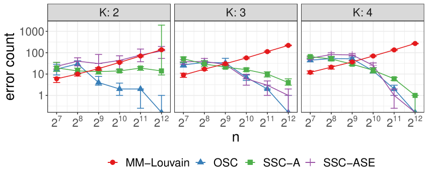
Figure 1: Median and IQR of community detection error. Communities are approximately balanced. Simulations were repeated 50 times for each sample size.

Given ground truth community labels, Fig. 2 shows that Algorithm 3 and the MLE-based plug-in estimators perform comparably, with root mean square error decaying at rate approximately $n^{-1/2}$ as $n$ increases.

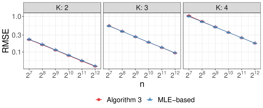
Figure 2: Median and IQR RMSE for edge probability matrices reconstructed from the outputs of Algorithm 3 (red) compared against outputs of an MLE-based method (blue) proposed in [17]. Simulations were repeated 50 times for each sample size. Communities were drawn to be approximately balanced.

4.2 Imbalanced Communities

Simulations performed in this section are the same as those in the previous section with the exception of the mixture parameters $\{\alpha_{1},...,\alpha_{K}\}$ used to draw community labels from the multinomial distribution. For these examples, we set the following parameters:

• Number of vertices $n=128,256,512,1024,2048,4096$

• Number of underlying communities $K=2,3,4$

• Mixture parameters $\alpha_{k}=\frac{k^{-1}}{\sum_{\ell=1}^{K}\ell^{-1}}$ for $k=1,...,K$

• Community labels $z_{k}\stackrel{{\scriptstyle\text{iid}}}{{\sim}}\mathrm{Multinomial}(\alpha_{1},...,\alpha_{K})$

• Within-group popularities $\lambda^{(kk)}\stackrel{{\scriptstyle\text{iid}}}{{\sim}}\mathrm{Beta}(2,1)$

• Between-group popularities $\lambda^{(k\ell)}\stackrel{{\scriptstyle\text{iid}}}{{\sim}}\mathrm{Beta}(1,2)$ for $k\neq\ell$

Fifty simulations were performed for each combination of $n$ and $K$. The results for community recovery and parameter estimations are presented in Fig. 3 and Fig. 4, respectively.

From Fig. 3 we once again see that the number of mislabeled vertices trending to $0$ for OSC. The performance of SSC-ASE is comparable to that of OSC for $K>2$ but is worse when $K=2$. Fig. 4 indicates that the parameter estimation error also decays at rate $n^{-1/2}$ similar to that in the balanced communities setting.

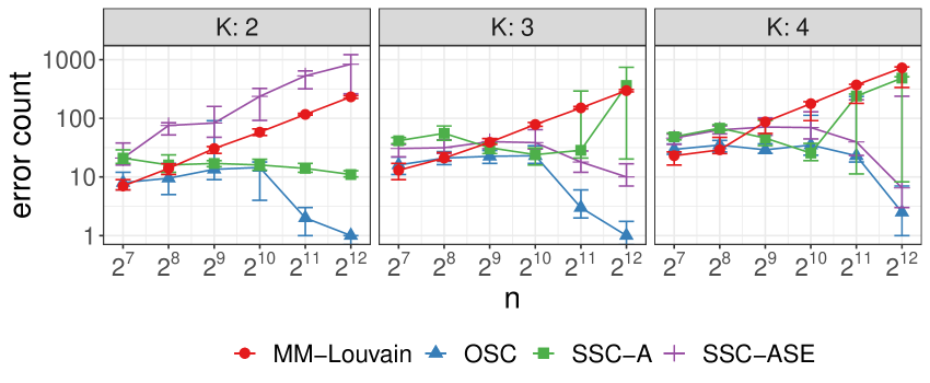
Figure 3: Median and IQR of community detection error. Communities are imbalanced. Simulations were repeated 50 times for each sample size.

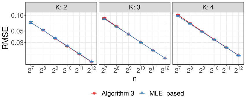
Figure 4: Median and IQR RMSE of edge probabilities derived from the outputs of Algorithm 3 (red) compared against an MLE-based method (blue) described in [17]. Simulations were repeated 50 times for each sample size. Communities were drawn to be imbalanced.

4.3 Disassortative Models

[16] demonstrated the power of applying GRDPG-based approaches to disassortative block models. Likewise, demonstrate that GRDPG-based algorithms OSC and SSC-ASE perform well on disassortative PABMs. Simulations performed in this section are the same as those in Section 4.1 with the exception of the distributions from which within and between-group popularity parameters are drawn. Here, we draw these parameters such that the expected value is $1/3$ for the within-group popularity parameters and $2/3$ for the between-group popularity parameters:

• Number of vertices $n=128,256,512,1024,2048,4096$

• Number of underlying communities $K=2,3,4$

• Mixture parameters $\alpha_{k}=\frac{k^{-1}}{\sum_{\ell=1}^{K}\ell^{-1}}$ for $k=1,...,K$

• Community labels $z_{k}\stackrel{{\scriptstyle\text{iid}}}{{\sim}}\mathrm{Multinomial}(\alpha_{1},...,\alpha_{K})$

• Within-group popularities $\lambda^{(kk)}\stackrel{{\scriptstyle\text{iid}}}{{\sim}}\mathrm{Beta}(1,2)$

• Between-group popularities $\lambda^{(k\ell)}\stackrel{{\scriptstyle\text{iid}}}{{\sim}}\mathrm{Beta}(2,1)$ for $k\neq\ell$

OSC, SSC-ASE, and SSC-A perform similarly on disassortative PABMs compared to the simulations in Sections 4.1 and 4.2. (Fig. 5 and 6).

Remark 5.

While we call the models in this section “disassortative”, it is our view that the assortative/disassortative distinction is not applicable to PABMs due to its flexibility. Unlike the SBM and DCBM, in the PABM, each vertex is free to have a higher affinity to its own community or to other communities, independent of each other. In other words, within the same community, $v_{i}$ may have a larger popularity parameter to its own community whereas $v_{j}$ may have a larger popularity parameter to a different community. Furthermore, when viewed as GRDPGs, the assortativity or disassortativity of SBMs and DCBMs affects whether $P$ is positive semidefinite, which affects ASE-based approaches to analyzing the graph [16], but in the full rank PABM, $P$ is never positive semidefinite and will always have $K(K+1)/2$ positive eigenvalues and $K(K-1)/2$ negative eigenvalues.

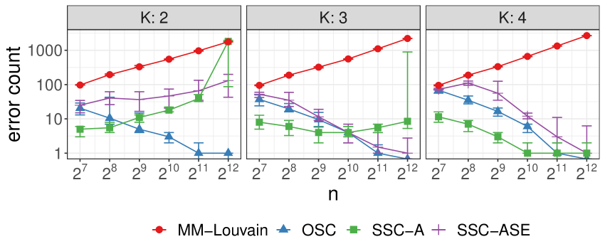
Figure 5: Median and IQR of community detection error. Communities are approximately balanced. Edge probabilities were drawn to be disassortative. Simulations were repeated 50 times for each sample size.

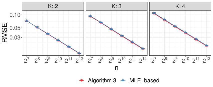
Figure 6: Median and IQR RMSE of edge probabilities derived from the outputs of Algorithm 3 (red) compared against an MLE-based method (blue) described in [17]. Simulations were repeated 50 times for each sample size. Communities were drawn to be approximately balanced. Edge probabilities were drawn to be disassortative.

5 Applications

In the first example, we applied OSC (Algorithm 1) to the Leeds Butterfly dataset [20] consisting of visual similarity measurements among 832 butterflies across 10 species. The graph was modified to match the example from [15]: Only the $K=4$ most frequent species were considered, and the similarities were discretized to $\{0,1\}$ via thresholding. Fig. 7 shows a sorted adjacency matrix sorted by the resultant clustering.

Comparing against the ground truth species labels, [15] report that SSC on the adjacency matrix achieves an adjusted Rand index of 73% in their implementation, whereas OSC achieves 92% and SSC on the ASE achieves 96%.

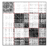
Figure 7: Adjacency matrix of the Leeds Butterfly dataset after sorting by the clustering outputted by OSC.

In the second example, we applied OSC to the British MPs Twitter network [8], the Political Blogs network [1], and the DBLP network [6, 9]. For this data analysis, we subsetted the data as described in [17] for their analysis of the same networks. Our methods slightly underperformed compared to modularity maximization, although performance is comparable. The run time of OSC is however much smaller than that of modularity maximization.

Figure 8: Adjacency matrices of (from left to right) the British MPs, Political Blogs, and DBLP networks after sorting by the clustering outputted by OSC.

Network	MM	SSC-ASE	OSC
British MPs	0.003	0.012	0.006
Political Blogs	0.050	0.187	0.062
DBLP	0.028	0.072	0.059

Table 1: Community detection error rates on the British MPs Twitter, Political Blogs, and DBLP networks using modularity maximization, sparse subspace clustering, and OSC.

In the third example (Fig. 9 and Table 2), we analyzed the Karantaka villages data studied by [2]. We chose the visitgo networks from villages 12, 31, and 46 at the household level. In these networks, each node is a household and each edge is an interaction between members of pairs of households. The label of interest is the religious affiliation. The networks were truncated to religions “1” and “2”, and vertices of degree 0 were removed. The villages were chosen based on there being an adequate number of nodes between households within each religion.

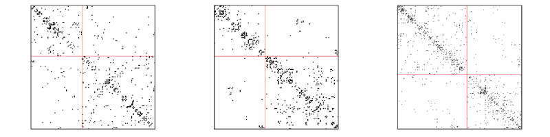
Figure 9: Adjacency matrix of the Karnataka villages data, arranged by the clustering produced by OSC (left). The villages studied here are, from left to right, 12, 31, and 46.

Network	MM	SSC-ASE	OSC
Village 12	0.270	0.291	0.227
Village 31	0.125	0.059	0.051
Village 46	0.052	0.069	0.056

Table 2: Community detection error rates for identifying household religion.

6 Discussion

Our central result states that the Popularity Adjusted Block Model is a special case of the Generalized Random Dot Product Graph. In particular, the PABM with $K$ communities is a GRDPG for which the communities are represented by mutually orthogonal $K$-dimensional subspaces of the $K^{2}$-dimensional latent space. This result extends previous results that connected the Stochastic Block Model and the Degree Corrected Block Model to Random Dot Product Graphs. Replacing RDPGs with GRDPGs is a critical step in this line of research, as a PABM is not necessarily a RDPG.

Because all Bernoulli Graphs are GRDPGs, it should be possible to invent and study new families of Bernoulli Graphs by characterizing them as special cases of GRDPGs and exploiting the latent structures that define them. The present work illustrates the power of this approach. We recover the latent structure of the PABM by Adjacency Spectral Embedding, then exploit that structure to improve statistical inference. Exploiting the fact that PABM communities correspond to orthogonal subspaces, we propose Orthogonal Spectral Clustering for community detection and demonstrate that the number of misclassified vertices approaches zero with high probability as the size of the graph increases. This is a stronger result than previously proposed algorithms [17], which only guarantee that the error rate (and not count) approaches zero asymptotically. Parameter estimation can be performed in a similar fashion using the ASE, for which we also prove that the per-parameter error approaches zero asymptotically.

A secondary benefit of the GRDPG approach is that the latent structure may be used to improve existing algorithms. For example, one algorithm for PABM community detection [15] relies on Sparse Subspace Clustering. The latent structure of the PABM provides a natural justification for SSC for the PABM and leads to an improvement over the previous implementation. The improved algorithm applies SSC to the ASE, and we prove that the ASE of the PABM obeys the Subspace Detection Property with high probability if the graph is large.

Finally, one might well inquire what one gains and what one sacrifices by assuming that a Bernoulli Graph is a PABM. The GRDPG model offers a plausible way to pursue this inquiry. Absent a known latent structure that can be exploited by specialized methods, the GRDPG-ASE approach transforms the problem of network community detection to the much-studied problem of clustering vectors in Euclidean space. Communities of vertices are defined as clusters of latent vectors. After ASE, a standard clustering algorithm, e.g., single linkage, is used to infer the communities. In future research, we intend to use such general algorithms as baselines and measure the efficiency of the PABM algorithms (and other specialized algorithms) by studying how much they improve on general algorithms when the specified latent structure obtains.

Appendix A Proofs of Theorem 3, Theorem 4, and Theorem 5

Let $V_{n}$ and $\hat{V}_{n}$ be the $n\times K^{2}$ matrices whose columns are the eigenvectors of $P$ and $A$ corresponding to the $K^{2}$ largest eigenvalues (in modulus), respectively. We first state an important technical lemma for bounding the maximum $\ell_{2}$ norm difference between the rows of $\hat{V}_{n}$ and $V_{n}$. See [4] and [16, Lemma 5 ] for a proof.

Lemma 1.

Let $A\sim\mathrm{PABM}(\{\lambda^{(k\ell\ell)}\}_{K})$ be a $K$-blocks PABM graph on $n$ vertices and let $V$ and $\hat{V}$ be the $n\times K^{2}$ matrices whose columns are the eigenvectors of $P$ and $A$ corresponding to the $K^{2}$ largest eigenvalues in modulus, respectively. Let $v_{i}^{\top}$ and $\hat{v}_{i}^{\top}$ denote the $i$th row of $V$ and $\hat{V}$, respectively. Then there exists a constant $c>1$ and an orthogonal matrix $W$ such that with high probability,

$$\max_{i}\|W\hat{v}_{i}-v_{i}\|=O\Big{(}\frac{\log^{c}n}{n\sqrt{\rho_{n}}}\Big{)}.$$

In particular we can take $c=1+\epsilon$ for any $\epsilon>0$.

Proof of Theorem 3.

Recall the notations in Lemma 1 and note that, under our assumption that the latent vectors $\lambda^{(k\ell)}$ are all homogeneous, we have $\max_{i}\|v_{i}\|=O(n^{-1/2})$.

Next recall Theorem 2; in particular $B_{ij}=nv_{i}^{\top}v_{j}$. We therefore have

$$\begin{split}\max_{ij}|\hat{B}_{ij}-B_{ij}|&=\max_{ij}n|\hat{v}_{i}^{\top}\hat{v}_{j}-v_{i}^{\top}v_{j}|\\ &\leq n\max_{ij}|\hat{v}_{i}^{\top}WW^{\top}\hat{v}_{j}-v_{i}^{\top}v_{j}|\\ &\leq n\max_{i,j}\Bigl{(}\|W^{\top}\hat{v}_{i}-v_{i}\|\times\|\hat{v}_{j}\|+\|W^{\top}\hat{v}_{j}-v_{j}\|\times\|v_{i}\|\Bigr{)}\\ &\leq n\Bigl{(}\max_{ij}\|W\hat{v}_{i}-v_{i}\|^{2}+\|W\hat{v}_{i}-v_{i}\|\times\|v_{j}\|+\|W\hat{v}_{j}-v_{j}\|\times\|v_{i}\|\Bigr{)}\\ &\leq n\max_{i}\|W\hat{v}_{i}-v_{i}\|^{2}+2n\max_{i}\|W\hat{v}_{i}-v_{i}\|\times\max_{j}\|v_{j}\|\\ &=O\Big{(}\frac{\log^{c}{n}}{n^{1/2}\rho_{n}^{1/2}}\Big{)}\end{split}$$

with high probability. Theorem 3 follows from the above bound together with the conclusion in Theorem 2 that $B_{ij}=0$ whenever vertices $i$ and $j$ belongs to different communities. ∎

We now provide a proof of Theorem 4. Our proof is based on verifying the sufficient conditions given in Theorem 6 of [21] under which sparse subspace clustering based on solving the optimization problem in Eq. (6) yields an affinity matrix $B=|C|+|C^{\top}|$ satisfying the subspace detection property of Definition 4. We first recall a few definitions used in [18] and [21]; for ease of exposition, these definitions are stated using the notations of the current paper and we will drop the explicit dependency on $n$ from our eigenvectors $\hat{V}$ of $A$ and $V$ of $P$.

Definition 5 (Inradius).

The inradius of a convex body $\mathcal{P}$, denoted by $r(\mathcal{P})$, is defined as the radius of the largest Euclidean ball inscribed in $\mathcal{P}$. Let $X$ be a $n\times d$ matrix with rows $x_{1},x_{2},\dots,x_{n}$. We then define, with a slight abuse of notation, $r(X)$ as the inradius of the convex hull formed by $\{\pm x_{1},\pm x_{2},\dots,\pm x_{n}\}$.

Definition 6 (Subspace incoherence).

Let $\hat{V}$ be the eigenvectors of $A$ corresponding to the $K^{2}$ largest eigenvalues in modulus. Let $\hat{V}^{(k)}$ denote the matrix formed by keeping only the rows of $\hat{V}$ corresponding to the $k^{th}$ community and let $\hat{V}^{(-k)}$ denote the matrix formed by omitting the rows of $\hat{V}$ corresponding to the $k^{th}$ community. Let $(\hat{v}_{i}^{(k)})^{\top}$ denote the $i$th row of $\hat{V}^{(k)}$ and $\hat{V}_{-i}^{(k)}$ be $\hat{V}^{(k)}$ with the $i^{th}$ row omitted. Let $V$, $V^{(k)}$, $V^{(-k)}$, and $v_{i}^{(k)}$ be defined similarly using the eigenvectors $V$ of $P$. Finally let $\mathcal{S}^{(k)}$ be the vector space spanned by the rows of $V^{(k)}$.

Now define $\nu_{i}^{(k)}$ for $k=1,2,\dots,K$ and $i=1,2,\dots,n_{k}$ as the solution of the following optimization problem

$$\nu_{i}^{(k)}=\max_{\eta}(\hat{v}_{i}^{(k)})^{\top}\eta-\frac{1}{2\lambda}\eta^{\top}\eta,\quad\text{subject to $\|V_{-i}^{(k)}\eta\|_{\infty}\leq 1$.}$$

Given $\nu_{i}^{(k)}$, let $\mathbb{P}_{\mathcal{S}^{(k)}}(\nu_{i}^{(k)})$ be the vector in $\mathbb{R}^{K^{2}}$ corresponding to the orthogonal projection of $\nu_{i}^{(k)}$ onto the vector space $\mathcal{S}^{(k)}$ and define the projected dual direction $w_{i}^{(k)}$ as

$$w_{i}^{(k)}=\frac{\mathbb{P}_{\mathcal{S}^{(k)}}(\nu_{i}^{(k)})}{\|\mathbb{P}_{\mathcal{S}^{(k)}}(\nu_{i}^{(k)})\|}.$$

Now let $W^{(k)}=\bigl{[}w_{1}^{(k)}\mid\cdots\mid w_{n_{k}}^{(k)}\bigr{]}^{\top}$ and define the subspace incoherence for $\hat{V}^{(k)}$ by

$$\mu^{(k)}=\mu(\hat{V}^{(k)})=\max\limits_{v\in V^{(-k)}}\|W^{(k)}v\|_{\infty}.$$

With the above definitions in place, we are now ready to state our proof of Theorem 4.

Proof of Theorem 4.

For a given $k=1,2\dots,K$, let $r^{(k)}=\min_{i}r(V_{-i}^{(k)})$ be inradius of the convex hull formed by the rows of $V_{-i}^{(k)}$ and let $r_{*}=\min_{k}r^{(k)}$. Then Theorem 6 in [21] states that there exists a $\lambda>0$ such that $\sqrt{n}\hat{V}$ satisfies the subspace detection property in Definition 4 whenever the following two conditions are satisfied

$$\mu^{(k)}<r^{(k)}\quad\text{for all $k=1,2,\dots,K$},$$ (10)

$$\max_{i}\|W\hat{v}_{i}-v_{i}\|\leq\min_{k}\frac{r_{*}(r^{(k)}-\mu^{(k)})}{2+7r^{(k)}}.$$ (11)

We now verify that for sufficiently large n, Eq. (10) and Eq. (11) holds with high probability.

Verifying Eq. (10). If $n$ is sufficiently large then there are enough vertices in each community $k$ so that $\mathrm{span}(V_{-i}^{(k)})=\mathcal{S}^{(k)}$ for all $i$ and hence $r^{(k)}=\min_{i}r(V_{-i}^{(k)})>0$ for all $k=1,2,\dots,K$.

Next, by Theorem 2 we have that the subspaces $\{\mathcal{S}^{(1)},\dots,\mathcal{S}^{(K)}\}$ are mutually orthogonal, i.e., $v^{\top}w=0$ for all $v\in\mathcal{S}^{(k)}$ and $w\in\mathcal{S}^{(\ell)}$ with $k\not=\ell$. Now let $z\in\mathbb{R}^{K^{2}}$ be arbitrary and let $\tilde{z}=\mathbb{P}_{\mathcal{S}^{(k)}}z$ be the projection of $z$ onto $\mathcal{S}^{(k)}$. We then have $v^{\top}\tilde{z}=0$ for all $v\in V^{(-k)}$. Because $z$ is arbitrary, this implies $\|W^{(k)}v\|_{\infty}=0$ for all $v\in V^{(-k)}$ and hence $\mu^{(k)}=0$ for all $k=1,2,\dots,K$. Therefore $\mu^{(k)}<r^{(k)}$ for all $k=1=2,\dots,K$ as desired.

Verifying Eq. (11). Let $\delta=\max_{i}\sqrt{n}\|W\hat{v}_{i}-v_{i}\|$. Then from Lemma 1, we have $\delta\stackrel{{\scriptstyle a.s.}}{{\to}}0$ and hence

$$\delta<\min_{k}\frac{r_{*}(r^{(k)}-\mu^{(k)})}{2+7r^{(k)}}$$

asymptotically almost surely.

In summary $\sqrt{n}\hat{V}$ satisfies the subspace detection property with probability converging to $1$ as $n\to\infty$. ∎

Remark 6.

Theorem 6 of [21] assumes that each row $v_{i}$ of $V$ has unit norm, i.e., $\|v_{i}\|=1$ for all $i$. This assumption has the effect of scaling the $r^{(k)}$ so that $r^{(k)}\leq 1$ for all $k=1,2,\dots,K$. We emphasize that this assumption has no effect on the proof of Theorem 4. Indeed, because $\mu^{(k)}=0$ for all $k$, as long as the rows of $V^{(k)}$ spans the subspace $\mathcal{S}^{(k)}$, then $ar^{(k)}>\mu^{(k)}$ for any scalar $a>0$.

Proof of Theorem 5.

Let $P$ be organized by community such that $P^{(k\ell)}$ denote the $n_{k}\times n_{\ell}$ matrix obtained by keeping only the rows of $P$ corresponding to vertices in community $k$ and the columns of $P$ corresponding to vertices in community $\ell$. We define $A^{(k\ell)}$ analogously. Recall that $P^{(k\ell)}=\lambda^{(k\ell)}(\lambda^{(\ell k)})^{\top}$ for all $k,\ell$. We now consider estimation of $P^{(k\ell)}$ for the cases when $k=\ell$ versus when $k\not=\ell$.

Case $k=l$. Let $P^{(kk)}=\sigma_{kk}^{2}u^{(kk)}(u^{(kk)})^{\top}$ be the singular value decomposition of $P^{(kk)}$. We can then define $\tilde{\lambda}^{(kk)}=\sigma_{kk}u^{(kk)}$. Now let $\hat{U}^{(kk)}\hat{\Sigma}^{(kk)}(\hat{U}^{(kk)})^{\top}$ be the singular value decomposition of $A^{(kk)}$, and let $\hat{\sigma}_{kk}^{2}\hat{u}^{(kk)}(\hat{u}^{(kk)})^{\top}$ be the best rank-one approximation of $A^{(kk)}$. Define $\hat{\lambda}^{(kk)}=\hat{\sigma}_{kk}\hat{u}^{(kk)}$. Then $\hat{\lambda}^{(kk)}$ is the adjacency spectral embedding approximation of $\lambda^{(kk)}$ and by Theorem 5 of [16], we have

$$\|\hat{\lambda}^{(kk)}-\lambda^{(kk)}\|_{\infty}=O\Bigl{(}\frac{\log n_{k}}{\sqrt{n_{k}}}\Bigr{)}$$

with high probability. Here $\|\cdot\|_{\infty}$ denote the $\ell_{\infty}$ norm of a vector.

Case $k\neq l$. Let $P^{(k\ell)}=\sigma_{k\ell}^{2}u^{(k\ell)}(v^{(k\ell)})^{\top}$ and $P^{(\ell k)}=\sigma_{kl}^{2}u^{(\ell k)}(v^{(\ell k)})^{\top}$ be the singular value decompositions and note that $\sigma_{k\ell}=\sigma_{\ell k}$, $u^{(k\ell)}=v^{(\ell k)}$, and $v^{(k\ell)}=u^{(\ell k)}$. Now define $\lambda^{(k\ell)}=\sigma_{k\ell}u^{(k\ell)}$ and $\lambda^{(\ell k)}=\sigma_{k\ell}v^{(k\ell)}$.

Next consider the Hermitian dilation

$$M^{(k\ell)}=2\begin{bmatrix}0&P^{(k\ell)}\\ P^{(\ell k)}&0\end{bmatrix}$$

which is a symmetric $(n_{k}+n_{\ell})\times(n_{k}+n_{\ell})$ matrix. The eigendecomposition of $M^{(k\ell)}$ is then

$$M^{(k\ell)}=\begin{bmatrix}u^{(k\ell)}&-u^{(k\ell)}\\ v^{(k\ell)}&v^{(k\ell)}\end{bmatrix}\times\begin{bmatrix}\sigma^{2}_{kl}&0\\ 0&-\sigma^{2}_{kl}\end{bmatrix}\times\begin{bmatrix}u^{(k\ell)}&-u^{(k\ell)}\\ v^{(k\ell)}&v^{(k\ell)}\end{bmatrix}^{\top}$$

Thus treating $M^{(k\ell)}$ as the edge probability matrix of a GRDPG, we have latent positions in $\mathbb{R}^{2}$ given by the $(n_{k}+n_{\ell})\times 2$ matrix

$$\Lambda^{(k\ell)}=\begin{bmatrix}\sigma_{k\ell}u^{(k\ell)}&\sigma_{k\ell}u^{(k\ell)}\\ \sigma_{k\ell}v^{(k\ell)}&-\sigma_{k\ell}v^{(k\ell)}\end{bmatrix}=\begin{bmatrix}\lambda^{(k\ell)}&\lambda^{(k\ell)}\\ \lambda^{(\ell k)}&-\lambda^{(\ell k)}\end{bmatrix}.$$

Now consider

$$\hat{M}^{(k\ell)}=\begin{bmatrix}0&A^{(k\ell)}\\ A^{(\ell k)}&0\end{bmatrix}$$

We can then view $\hat{M}^{(k\ell)}$ as an adjacency matrix drawn from the edge probabilities matrix $M^{(k\ell)}$. Now suppose that the adjacency spectral embedding of $\hat{M}^{(k\ell)}$ is represented as the $(n_{k}+n_{\ell})\times 2$ matrix

$$\hat{\Lambda}^{(k\ell)}=\begin{bmatrix}\hat{\lambda}^{(k\ell)}&\hat{\lambda}^{(k\ell)}\\ \hat{\lambda}^{(\ell k)}&-\hat{\lambda}^{(\ell k)}\end{bmatrix}$$

where each $\hat{\lambda}^{(k\ell)}$ is defined as in Algorithm 3. Then by Theorem 5 of [16], there exists an indefinite orthogonal transformation $W^{*}$ such that, with high probability,

$$\max_{i}|W^{*}\hat{\Lambda}_{i}^{(k\ell)}-\Lambda_{i}^{(k\ell)}\|=O\Bigl{(}\frac{\log(n_{k}+n_{\ell})}{\sqrt{n_{k}+n_{\ell}}}\Bigr{)}$$

with high probability. Here $\Lambda_{i}^{(k\ell)}$ and $\hat{\Lambda}_{i}^{(k\ell)}$ denote the $i$th rows of $\Lambda^{(k\ell)}$ and $\hat{\Lambda}^{(k\ell)}$, respectively.

Furthermore, by looking at the proof of Theorem 5 in [16], we see that $W^{*}$ is also blocks diagonal with $2$ blocks where the positive eigenvalues of $M^{(k\ell)}$ forming a block and the negative eigenvalues of $M^{(k\ell)}$ forming the remaining block. Because $M^{(k\ell)}$ has one positive eigenvalue and one negative eigenvalue, we see that $W^{*}$ is necessarily of the form $W^{*}=\Bigl{[}\begin{smallmatrix}1&0\\ 0&-1\end{smallmatrix}\Bigr{]}$ Using this form for $W^{*}$, we obtain

$$\max\{\|\hat{\lambda}^{(k\ell)}-\lambda^{(k\ell)}\|_{\infty},\|\hat{\lambda}^{(\ell k)}-\lambda^{(\ell k)}\|_{\infty}\}=O\Bigl{(}\frac{\log(n_{k}+n_{\ell})}{\sqrt{n_{k}+n_{\ell}}}\Bigr{)}$$

with high probability. Combining this bound with the bound for $\|\hat{\lambda}^{(kk)}-\lambda^{(kk)}\|_{\infty}$ given above yields Eq. (8) in Theorem 5. ∎

References

- [1] Lada A. Adamic and Natalie Glance “The Political Blogosphere and the 2004 U.S. Election: Divided They Blog” In Proceedings of the 3rd International Workshop on Link Discovery, 2005, pp. 36–43
- [2] A. Banerjee, A. G. Chandrasekhar, E. Duflo and M. O. Jackson “The Diffusion of Microfinance”, Harvard Dataverse, 2013 URL: https://doi.org/10.7910/DVN/U3BIHX
- [3] M. Belkin and P. Niyogi “Laplacian eigenmaps for dimensionality reduction and data representation” In Neural Computation 15, 2003, pp. 1373–1396
- [4] J. Cape, M. Tang and C. E. Priebe “Signal-plus-noise matrix models: eigenvector deviations and fluctuations” In Biometrika 106, 2019, pp. 243–250
- [5] Ehsan Elhamifar and Rene Vidal “Sparse subspace clustering” In 2009 IEEE Conference on Computer Vision and Pattern Recognition, 2009, pp. 2790–2797
- [6] J. Gao et al. “Graph-based Consensus Maximization among Multiple Supervised and Unsupervised Models” In Advances in Neural Information Processing Systems 22, 2009, pp. 585–593
- [7] E. N. Gilbert “Random Graphs” In The Annals of Mathematical Statistics 30 Institute of Mathematical Statistics, 1959, pp. 1141 –1144
- [8] D. Greene and P. Cunningham “Producing a Unified Graph Representation from Multiple Social Network Views” In Proceedings of the 5th Annual ACM Web Science Conference, 2013, pp. 118–121
- [9] M. Ji et al. “Graph Regularized Transductive Classification on Heterogeneous Information Networks” In Machine Learning and Knowledge Discovery in Databases Springer, 2010, pp. 570–586
- [10] B. Karrer and M. E. J. Newman “Stochastic blockmodels and community structure in networks” In Physical Review E 83 American Physical Society (APS), 2011
- [11] C. M. Le, E. Levina and R. Vershynin “Optimization via low-rank approximation for community detection in networks” In Annals of Statistics 44, 2016, pp. 373–400
- [12] G. Liu et al. “Robust recovery of subspace structures by low-rank representation” In IEEE Transactions on Pattern Analysis and Machine Intelligence 35, 2013, pp. 171–184
- [13] F. Lorrain and H. C. White “Structural equivalence of individuals in social networks” In The Journal of Mathematical Sociology 1, 1971, pp. 49–80
- [14] B. Nasihatkon and R. Hartley “Graph connectivity in sparse subspace clustering” In Computer Vision and Pattern Recognition, 2011, pp. 2137–2144
- [15] M. Noroozi, R. Rimal and M. Pensky “Estimation and clustering in popularity adjusted block model” In Journal of the Royal Statistical Society, Series B. 83, 2021, pp. 293–317
- [16] P. Rubin-Delanchy, J. Cape, M. Tang and C. E. Priebe “A statistical interpretation of spectral embedding: the generalised random dot product graph” arXiv: 1709.05506, 2017 arXiv:1709.05506 [stat.ML]
- [17] S. Sengupta and Y. Chen “A block model for node popularity in networks with community structure” In Journal of the Royal Statistical Society, Series B. 80, 2018, pp. 365–386
- [18] M. Soltanolkotabi and E. J. Candés “A geometric analysis of subspace clustering with outliers” In Annals of Statistics 40, 2012, pp. 2195–2238
- [19] D. L. Sussman, M. Tang, D. E. Fishkind and C. E. Priebe “A Consistent Adjacency Spectral Embedding for Stochastic Blockmodel Graphs” In Journal of the American Statistical Association 107, 2012, pp. 1119–1128
- [20] B. Wang et al. “Network enhancement as a general method to denoise weighted biological networks” In Nature Communications 9 Springer ScienceBusiness Media LLC, 2018
- [21] Y.-X. Wang and H. Xu “Noisy Sparse Subspace Clustering” In Journal of Machine Learning Research 17, 2016, pp. 1–41
- [22] S. J. Young and E. R. Scheinerman “Random Dot Product Graph Models for Social Networks” In Algorithms and Models for the Web-Graph Springer, 2007, pp. 138–149