Deep Reinforcement Learning for Equal Risk Pricing and Hedging under Dynamic Expectile Risk Measures

Abstract

Recently equal risk pricing, a framework for fair derivative pricing, was extended to consider dynamic risk measures. However, all current implementations either employ a static risk measure that violates time consistency, or are based on traditional dynamic programming solution schemes that are impracticable in problems with a large number of underlying assets (due to the curse of dimensionality) or with incomplete asset dynamics information. In this paper, we extend for the first time a famous off-policy deterministic actor-critic deep reinforcement learning (ACRL) algorithm to the problem of solving a risk averse Markov decision process that models risk using a time consistent recursive expectile risk measure. This new ACRL algorithm allows us to identify high quality time consistent hedging policies (and equal risk prices) for options, such as basket options, that cannot be handled using traditional methods, or in context where only historical trajectories of the underlying assets are available. Our numerical experiments, which involve both a simple vanilla option and a more exotic basket option, confirm that the new ACRL algorithm can produce 1) in simple environments, nearly optimal hedging policies, and highly accurate prices, simultaneously for a range of maturities 2) in complex environments, good quality policies and prices using reasonable amount of computing resources; and 3) overall, hedging strategies that actually outperform the strategies produced using static risk measures when the risk is evaluated at later points of time.

Keywords Reinforcement learning, Option pricing, risk hedging, expectile risk measures, incomplete market

1 Introduction

Derivative pricing remains to be a challenging problem in finance when the markets are incomplete and the derivatives are dependent on multiple underlying assets. The incompleteness of a market implies that the price of a derivative cannot be uniquely determined by the standard replication argument, as in such a market no self-financing hedging strategy exists that can perfectly replicate the payoffs of the derivative. Many mechanisms have been proposed for pricing in an incomplete market but most were developed from the perspective of a single trader. Unfortunately, a price that is set only according to one party’s interest, e.g. a super-replication price that a seller may wish to charge, may not be acceptable to the buyer and thus does not represent a plausible transaction price. Recently, a new pricing scheme, known as Equal Risk Pricing (ERP), was proposed by Guo and Zhu (2017) and further adapted to convex risk measures in the work of Marzban et al. (2020).

The scheme of ERP is built upon the idea of modelling separately the risk exposure of the buyer and the seller of a derivative, and seeking a price that ensures that the risk exposure of both parties is the same under their respective optimal self-financing hedging strategy. The price generated from ERP thus has the merit of fairness to both parties. While ERP has its conceptual appeal, there remains a gap between its general construct and the actual implementation. In particular, as shown in Marzban et al. (2020), great care must be taken to define properly how risk should be measured in a dynamic hedging setting in order to obtain hedging problems that are operationally meaningful and computationally solvable. The work of Marzban et al. (2020) provides necessary analysis for solving the equal risk pricing and hedging problem based on dynamic programming (DP). It is known however that DP suffers from the issue of the curse of dimensionality, which restricts the applicability of the results in Marzban et al. (2020). In addition, DP assumes the knowledge of a stochastic model that precisely captures the dynamics of the markets, which may not be available in practice.

In the past decade, Deep Reinforcement Learning (DRL) has proven to be a powerful tool for solving dynamic optimization problems when the number of state variables is large and/or when no stochastic model is known for the underlying system dynamics. In particular, the recent works of Carbonneau and Godin (2020) and Carbonneau and Godin (2021) are the first that apply DRL to solve ERP problems and they demonstrate the possibility of pricing a broad range of over-the-counter options such as basket options. Unfortunately, the DRL approaches proposed in Carbonneau and Godin (2020) and Carbonneau and Godin (2021) can only be used in settings where the risk is measured according to a static risk measure. This raises the serious issue that the hedging problem exploited by the ERP could be time inconsistent, i.e. the hedging decisions planned for future state of the world may not be considered optimal anymore once the state is visited. The violation of time consistency implies that equal risk prices calculated based on static risk measures will assume a hedging policy that cannot be implemented in practice, and thus are optimistically biased. From a numerical perspective, employing a static risk mesure in ERP also limits the type of DRL algorithms that can be used to solve each party’s hedging problem. Specifically, the authors of Carbonneau and Godin (2020) and Carbonneau and Godin (2021) employ a policy optimization scheme, a.k.a. Actor-Only RL (AORL) algorithm (see Williams (1992) as an example of this method), while other approaches such as critic-only or actor-critic algorithms (such as Mnih et al. (2015) and Silver et al. (2014) respectively) that rely on an equivalent DP formulation remain out of reach.

In this paper, we seek to develop a DRL approach for solving a class of time-consistent ERP problems. It is known that to ensure time consistency, a dynamic risk measure should be employed to measure risk in a recursive fashion. In particular, motivated by the theory of coherent risk measures, which identifies expectile risk measures as the only elicitable coherent risk measures, we propose in this paper the use of dynamic expectile risk measures to formulate time consistent ERP problems. The dynamic nature of risk measures suggests the consideration of an Actor-Critic RL (ACRL) algorithm for solving the hedging problem. It turns out that the elicitability property of expectile risk measures facilitates greatly the design of a model-free ACRL algorithm. The convergence of this algorithm is also greatly improved due to the translation invariance property of the risk measures.

Overall, we may summarize the contribution of this paper as follows:

• We present the first model-free DRL based algorithm for computing equal risk prices that rely on option hedging strategies that are time-consistent. To reinforce the importance of this contribution, we in fact demonstrate using a simple single asset two-period horizon option pricing problem how equal risk prices might suffer from an optimistic bias when static risk measures are used (as in Carbonneau and Godin (2020) and Carbonneau and Godin (2021)). A side benefit from pricing an option with maturity $T$ using dynamic risk measures will be that we will easily obtain equal risk prices for any other maturity $T^{\prime}<T$.

• The ACRL algorithm that we propose is the first model-free DRL algorithm to naturally extend the famous off-policy deterministic actor-critic method presented in Silver et al. (2014) to the risk averse setting. Unlike the ACRL proposed in Tamar et al. (2015) and Huang et al. (2021) for risk-averse DRL, which can employ up to five neural networks, our algorithm will only require two deep neural networks: a policy network (actor) and a Q network (critic). While our policy network will be trained following a stochastic gradient procedure similar to Silver et al. (2014), to the best of our knowledge we are the first to leverage the elicitability property (i.e. existence of a scoring function) of expectile risk measures and to propose a procedure for training the “risk-to-go” Q network that is also based on stochastic gradient descent.

• We perform a comprehensive evaluation of the training efficiency, quality of option hedging strategies, and quality of equal risk prices obtained using our ACRL algorithm on a synthetic multi-asset geometric Brownian motion market model. In the simple case of vanilla option pricing, we provide empirical evidence that ACRL provides nearly optimal hedging policies, and highly accurate prices, simultaneously for a range of maturities. The latter is in sharp contrast with approaches, such as in Carbonneau and Godin (2021), that employ time inconsistent risk measures and produce investment strategies that are visibly outperformed by the ACRL strategy in terms of the risk measured as time to maturity reduces. This phenomenon is also observed, although less prominently, in the context of a basket option over 5 underlying assets, where good quality policies and prices are obtained using our ACRL algorithm using a reasonable amount of computing resources.

The rest of this paper is organized as follows. Section 2 introduces equal risk pricing and illustrates using a simple two-period pricing problem the practical issues related to using static risk measures for option hedging and pricing. Section 3 adapts the ERP framework to the case of a dynamic expectile risk measure and proposes the new ACRL algorithm. Finally, Section 4 presents and discusses our numerical experiments.

2 Equal risk pricing and hedging under coherent risk measures

In this section, we provide a brief overview of ERP under coherent risk measures based on the recent work of Marzban et al. (2020). We pay particular attention to the issue of time (in)consistency by presenting an example that demonstrates numerically that employing a time-inconsistent static risk measure can lead to an under-evaluation of the risk to which each party are actually exposed in practice.

2.1 ERP under coherent risk measures

The problem of ERP can be formalized as follows. Consider a frictionless market, i.e. no transaction cost, tax, etc, that contains $m$ risky assets, and a risk-free bank account with zero interest rate. Let $\mathbf{S}_{t}:\Omega\rightarrow\mathbb{R}^{m}$ denote the values of the risky assets adapted to a filtered probability space $(\Omega,\mathcal{F},\mathbb{F}:=\{\mathcal{F}_{t}\}_{t=0}^{T},\mathbb{P})$, i.e. each $\mathbf{S}_{t}$ is $\mathcal{F}_{t}$ measurable. It is assumed that $\mathbf{S}_{t}$ is a locally bounded real-valued semi-martingale process and that the set of equivalent local martingale measures is non-empty (i.e. no arbitrage opportunity). The set of all admissible self-financing hedging strategies with the initial capital $p_{0}\in\mathbb{R}$ is shown by $\mathcal{X}(p_{0})$:

$$\mathcal{X}(p_{0})=\left\{X:\Omega\rightarrow\mathbb{R}^{T}\left|\exists\{\boldsymbol{\xi}_{t}\}_{t=0}^{T-1},\quad X_{t}=p_{0}+\sum_{t^{\prime}=0}^{t-1}\boldsymbol{\xi}_{t^{\prime}}^{\top}\Delta\mathbf{S}_{t^{\prime}+1},\quad\forall t=1,\dots,T\right.\right\}\,,$$

where $\Delta\mathbf{S}_{t+1}:=\mathbf{S}_{t+1}-\mathbf{S}_{t}$, the hedging strategy $\boldsymbol{\xi}_{t}\in\mathbb{R}^{m}$ is a vector of random variables adapted to the filtration $\mathbb{F}$ and captures the number of shares of each of the risky assets held in the portfolio during the period $[t,\;t+1]$, $\boldsymbol{\xi}_{t}^{\top}\Delta\mathbf{S}_{t^{\prime}+1}$ is the inner product of the two random vectors, and $X_{t}$ is the accumulated wealth.

Let $F(\{\mathbf{S}_{t}\}_{t=1}^{T})$ denote the payoff of a derivative. Throughout this paper, we assume $F(\{\mathbf{S}_{t}\}_{t=1}^{T})$ admits the formulation of $F(\mathbf{S}_{T},\mathbf{Y}_{T})$ where $\mathbf{Y}_{t}$ is an auxiliary fixed-dimensional stochastic process that is $\mathcal{F}_{t}$-measurable. This class of payoff functions is common in the literature, (see for example Bertsimas et al. (2001) and Marzban et al. (2020)). The problem of ERP is defined based on the following two hedging problems that seek to minimize the risk of hedging strategies, one is for the writer and the other is for the buyer of the derivative:

(Writer) $$\varrho^{w}(p_{0})=\inf_{X\in\mathcal{X}(p_{0})}\rho^{w}(F(\mathbf{S}_{T},\mathbf{Y}_{T})-X_{T})$$ (1)

(Buyer) $$\varrho^{b}(p_{0})=\inf_{X\in\mathcal{X}(-p_{0})}\rho^{b}(-F(\mathbf{S}_{T},\mathbf{Y}_{T})-X_{T})\,,$$ (2)

where $\rho^{w}$ and $\rho^{b}$ are two risk measures that capture respectively the writer and the buyer’s risk aversion. In words, equation (1) describes a writer that is receiving $p_{0}$ as the initial payment and implements an optimal hedging strategy for the liability captured by $F(\mathbf{S}_{T},\mathbf{Y}_{T})$. On the other hand, in (2) the buyer is assumed to borrow $p_{0}$ in order to pay for the option and then to manage a portfolio that will minimize the risks associated to his final wealth $F(\mathbf{S}_{T},\mathbf{Y}_{T})+X_{T}$. With equations (1) and (2), ERP defines a fair price $p_{0}^{*}$ as the value of an initial capital that leads to the same risk exposure to both parties, i.e.

$$\rho^{w}(p_{0}^{*})=\rho^{b}(p_{0}^{*}).$$

Motivated by the theory of coherent risk measures (Artzner et al. (1999)), Marzban et al. (2020) study the ERP problem by imposing the property of coherency to the risk measures $\rho^{w}$ and $\rho^{b}$. Namely, a risk measure is said to be coherent if it satisfies the following five conditions:

• Monotonicity: if $X\leq Z\quad a.s.$ then $\rho(X)\leq\rho(Z)$

• Subadditivity: $\rho(X+Z)\leq\rho(X)+\rho(Z)$

• Positive homogeneity: If $\lambda\geq 0$, then $\rho(\lambda X)=\lambda\rho(X)$

• Translation invariance: If $m\in\mathbb{R}$, then $\rho(X+m)=\rho(X)+m$

• Normalized risk: $\rho(0)=0$.

It is well known that Value-at-Risk (VaR), a risk measure commonly applied in financial risk management, is not coherent, whereas its convex counterpart, namely Conditional Value-at-Risk (CVaR) is coherent. The application of CVaR in ERP can be found for example in Carbonneau and Godin (2020). As one of the key results in ERP, Marzban et al. (2020) establishes that an equal risk price $p_{0}^{*}$ can actually be found by solving the writer and buyer’s hedging problem with no initial payment, i.e. (1) and (2), separately. Namely, it can be calculated by the following result.

Theorem 2.1.

Let $\rho^{w}$ and $\rho^{b}$ be two coherent risk measures. In the case where the equal risk price $p_{0}^{*}$ exists, it can be calculated by

$$p_{0}^{*}=(\varrho^{w}(0)-\varrho^{b}(0))/2\,,$$

when $\infty>\varrho^{w}(0)\geq\varrho^{b}(0)>-\infty$.

2.2 The issue of time inconsistency

As briefly mentioned in the introduction, measuring risk in a dynamic setting requires additional care. The use of a coherent risk measure, without any further adaptation to a dynamic setting, can lead to solutions that suffer from the issue of time inconsistency. The goal of this section is to carefully demonstrate this point by presenting a numerical example that quantifies the impact of time inconsistency. Our demonstration is inspired by the work of Rudloff et al. (2014), where the impact of time inconsistency is discussed in a portfolio management problem. Here, we present an example based on a vanilla option hedging problem.

In this example, we consider a stock price process modelled by a simple two-stage trinomial tree. Specifically, the horizon spans $t\in\{0,1,2\}$ and the probability space $(\Omega,\mathcal{F},\mathbb{P})$ is such that $\Omega=\{\omega_{i}\}_{i=1}^{9}$, $\mathcal{F}_{1}:=\sigma(\{\{\omega_{i}\}_{i=1}^{3},\{\omega_{i}\}_{i=4}^{6},\{\omega_{i}\}_{i=7}^{9}\})$, and all outcomes are equiprobable. The market contains a risk-free asset (with a risk-free rate of zero) and a risky asset $S$ which are used to hedge a vanilla at-the-money call option on $S_{2}$ with strike price $K:=S_{0}$. The details of the price process is shown in Table 1. For simplicity, we set the initial capital for hedging to zero and employ a $\mbox{CVaR}_{60\%}$ risk measure for hedging.

When hedging the call-option using a static CVaR measure, the writer of the option solves the following two-period optimization model:

$$\min_{\xi_{0},\xi_{1}}\quad \mbox{CVaR}_{60\%}((S_{2}(\omega)-K)^{+}-(S_{1}(\omega)-S_{0})\xi_{0}-(S_{2}(\omega)-S_{1}(\omega))\xi_{1}(\omega))$$ (3)

where $(y)^{+}:=\max(y,0)$ and $K:=S_{0}$. The optimal solution of this problem will prescribe purchasing 0.93 shares of the risky asset at time 0, i.e. $\xi_{0}=0.9341$, using money borrowed at the risk-free rate (see Table 1 for the optimal shares to hold at $t=1$). The resulting $\mbox{CVaR}_{60\%}$ is $26.36$, implying that if the writer charges the buyer with a price above $26.36$, the writer would consider the price being sufficient to cover the hedged risk of this call option.

Note that in the risk averse hedging problem (3), it is not clear what motivates the writer of the option to implement the prescribed hedging strategy once new information is revealed at time $t=1$. In particular, he/she might be curious to compare the prescribed strategy with the strategy that minimizes the CVaR from the new perspective at $t=1$, i.e., the following hedging problem:

$$\min_{\bar{\xi}_{1}}\quad \mbox{CVaR}_{\bar{\alpha}_{1}}((S_{2}(\omega)-K)^{+}-(S_{1}(\omega)-S_{0})\xi_{0}^{*}-(S_{2}(\omega)-S_{1}(\omega))\bar{\xi}_{1}(\omega)|\mathcal{F}_{1})\,,$$ (4)

where $\bar{\alpha}_{1}:=60\%$ and where $\xi_{0}^{*}=0.9341$, i.e. the optimal first stage solution in (3).

Table 1 presents the optimal conditional hedging strategy $\bar{\xi}_{1}^{*}$ as a function of the information revealed by $\mathcal{F}_{1}$. While it does appear that $\bar{\xi}_{1}^{*}$ agrees with $\xi_{1}^{*}$ when $\omega\in\{\omega_{i}\}_{i=1}^{3}$, the investment in the risky asset ends up significantly reduced in the other two sets of outcomes. More importantly, we established that in order to motivate the prescribed hedging strategy $\xi_{1}^{*}$, the risk aversion level used in problem (4) would need to be in the range of $[0.4580,\;0.4585]$, when $\omega\in\{\omega_{i}\}_{i=4}^{6}$, or $[0.1992,\;0.2]$, when $\omega\in\{\omega_{i}\}_{i=7}^{9}$. This confirms that $\xi^{*}$ is likely to be perceived as overly risky given the information revealed at time $t=1$. Ultimately, in the likely case where the writer decides to replace $\xi_{1}^{*}$ with $\bar{\xi}_{1}^{*}$, one can establish that the overall exposition to risk from the perspective of $t=0$ should have rather been estimated to 27.94 instead of 26.36. This implies that employing a static risk measure here underestimated the necessary coverage capital by $6\%$.

While this issue of time consistency has been discussed significantly in the recent years, a common approach to overcome it is to employ a so-called dynamic risk measure as will be done in the following section. In the context of this example, this would reduce to replacing problem (3) with:

$$\min_{\xi_{0},\xi_{1}}\quad \mbox{CVaR}_{\alpha}(\;\mbox{CVaR}_{\alpha}((S_{2}(\omega)-K)^{+}-(S_{2}(\omega)-S_{1}(\omega))\xi_{1}(\omega)-(S_{1}(\omega)-S_{0})\xi_{0}|\mathcal{F}_{1}(\omega))\;)\,,$$ (5)

where $\alpha$ can be chosen to characterize the right level of risk aversion for the “dynamic conditional value-at-risk measure”. This formulation ensures that the prescribed policy at time $t=1$ remains optimal (according to problem (4)) at the moment where it is actually implemented thus preventing the necessary coverage capital from being under estimated.

Table 1: Example of a time inconsitent hedging strategy obtained from employing a static risk measure. $\xi^{*}$ is obtained by solving problem (3), $\bar{\alpha}_{1}$ is the risk aversion level that motivates $\xi_{1}^{*}$ at $t=1$, $\bar{\xi}_{1}^{*}$ is the actual investment prescribed by $\mbox{CVaR}_{60\%}$ at $t=1$.

Atoms	Price process			Time inconsistent			Optimal conditional
of $\mathcal{F}_{1}$				hedging strategy			hedging strategy
	$S_{0}(\omega)$	$S_{1}(\omega)$	$S_{2}(\omega)$	$\xi^{*}_{0}$	$\xi^{*}_{1}(\omega)$	$\bar{\alpha}_{1}(\xi^{*})$	$\bar{\xi}^{*}_{1}(\omega)$
$\omega\in\{\omega_{i}\}_{i=1}^{3}$	100	150	{270,150,75}	0.9341	0.8718	[0.4580,1.0000]	0.8718
$\omega\in\{\omega_{i}\}_{i=4}^{6}$	100	100	{180,100,50}	0.9341	0.7665	[0.4580,0.4585]	0.6154
$\omega\in\{\omega_{i}\}_{i=7}^{9}$	100	80	{120,80,64}	0.9341	0.5000	[0.1992,0.2000]	0.3571

3 ERP under dynamic expectile risk measure and an actor-critic algorithm

While time consistent ERP problems can be formulated by employing dynamic risk measures and be calculated, in principle, by solving a set of dynamic programming (DP) equations (Marzban et al. (2020)), there remains the challenge of determining which dynamic risk measure one should employ and how these equations might be solved in high dimension, i.e. multiple underlying assets. In this section, we address the two issues by first motivating the use of dynamic expectile risk measures to formulate time consistent ERP hedging problems and then presenting a Deep Reinforcement Learning approach (DRL) for approximately solving this problems.

3.1 Dynamic expectile risk measures and DP equations

Expectile has been proposed in the recent literature (see Bellini and Bignozzi (2015)) as a replacement of VaR and CVaR given that it is not only coherent but also elicitable. It is known that VaR is not coherent but is elicitable, whereas CVaR is coherent but is not elicitable. A risk measure is said to be elicitable if it can be expressed as the minimizer of a certain scoring function, and this property is found to be critical in practice due to the need of backtesting (Chen, 2018). In fact, expectile is the only elicitable coherent risk measure. Recall the following definition of expectile.

Definition 3.1.

(Bellini and Bernardino (2017)) The $\tau-$expectile of a random liability $X$ is defined as:

$$\bar{\rho}(X):=\arg\min_{q}\,\tau\mathbb{E}\left[(q-X)_{+}^{2}\right]+(1-\tau)\mathbb{E}\left[(q-X)_{-}^{2}\right]\,.$$

Like CVaR, expectile covers at one extreme the case of risk-neutrality, i.e. with $\tau=1/2$, and at the other extreme the case of converging towards the worst-case risk, i.e. as $\tau\rightarrow 1$. Thus, expectile also allows for modelling a wide spectrum of risk aversion. Using expectile as the basis, we define its dynamic version as follows.

Definition 3.2.

A dynamic recursive expectile risk measure takes the form:

$$\rho(X):=\bar{\rho}_{0}(\bar{\rho}_{1}(\dots\bar{\rho}_{T-1}(X)))\,,$$

where each $\bar{\rho}(\cdot)$ is an expectile risk measure that employs the conditional distribution based on $\mathcal{F}_{t}$. Namely,

$$\bar{\rho}_{t}(X_{t+1}):=\arg\min_{q}\,\tau\mathbb{E}\left[(q-X_{t+1})_{+}^{2}|\mathcal{F}_{t}\right]+(1-\tau)\mathbb{E}\left[(q-X_{t+1})_{-}^{2}|\mathcal{F}_{t}\right]$$

where $X_{t+1}$ a random liability measureable on $\mathcal{F}_{t+1}$.

We apply dynamic expecile risk measures to formulate the two hedging problems in ERP. By further imposing the following assumption that there exists a sufficient statistic process $\psi_{t}$ such that $\{(\mathbf{S}_{t},\mathbf{Y}_{t},\psi_{t})\}_{t=0}^{T}$ satisfies the Markov property, we can obtain compact dynamic equations for them.

Assumption 3.1.

[Markov property] There exists a sufficient statistic process $\psi_{t}$ adapted to $\mathbb{F}$ such that $\{(\mathbf{S}_{t},\mathbf{Y}_{t},\psi_{t})\}_{t=0}^{T}$ is a Markov process relative to the filtration $\mathbb{F}$. Namely, ${\mathbb{P}}((\mathbf{S}_{t+s},\mathbf{Y}_{t+s},\psi_{t+s})\in\mathcal{A}|\mathcal{F}_{t})={\mathbb{P}}((\mathbf{S}_{t+s},\mathbf{Y}_{t+s},\psi_{t+s})\in\mathcal{A}|\mathbf{S}_{t},\mathbf{Y}_{t},\psi_{t})$ for all $t$, for all $s\geq 0$, and all sets $\mathcal{A}$.

In particular, based on Proposition 3.1 and the examples presented in section 3.3 of Marzban et al. (2020), together with the fact that both $\rho^{w}$ and $\rho^{b}$ are dynamic recursive expectile risk measures, the Markovian assumption allows us to conclude that the ERP can be calculated using two sets of dynamic programming equations. Specifically, on the writer side, we can define

$$V^{w}_{T}(\mathbf{S}_{T},\mathbf{Y}_{T},\psi_{T}):=F(\mathbf{S}_{T},\mathbf{Y}_{T})\,,$$

and recursively

$$V^{w}_{t}(\mathbf{S}_{t},\mathbf{Y}_{t},\psi_{t}):=\inf_{\boldsymbol{\xi}_{t}}\bar{\rho}(-\boldsymbol{\xi}_{t}^{\top}\Delta\mathbf{S}_{t+1}+V_{t+1}^{w}(S_{t}+\Delta\mathbf{S}_{t+1},\mathbf{Y}_{t}+\Delta Y_{t+1},\psi_{t+1})|\mathbf{S}_{t},\mathbf{Y}_{t},\psi_{t})\,,$$

where $\bar{\rho}(\cdot|\mathbf{S}_{t},\mathbf{Y}_{t},\psi_{t})$ is the expectile risk measure that uses $\mathbb{P}(\cdot|\mathbf{S}_{t},\mathbf{Y}_{t},\psi_{t})$. This leads to considering $\varrho^{w}(0)=V^{w}_{0}(\mathbf{S}_{0},\mathbf{Y}_{0},\psi_{0})$. On the other hand, for the buyer we similarly define:

$$V^{b}_{T}(\mathbf{S}_{T},\mathbf{Y}_{T},\psi_{T}):=-F(\mathbf{S}_{T},\mathbf{Y}_{T})\,,$$

and

$$V^{b}_{t}(\mathbf{S}_{t},\mathbf{Y}_{t},\psi_{t}):=\inf_{\boldsymbol{\xi}_{t}}\bar{\rho}(-\boldsymbol{\xi}_{t}^{\top}\Delta\mathbf{S}_{t+1}+V_{t+1}^{b}(\mathbf{S}_{t}+\Delta\mathbf{S}_{t+1},\mathbf{Y}_{t}+\Delta\mathbf{Y}_{t+1},\psi_{t+1})|\mathbf{S}_{t},\mathbf{Y}_{t},\psi_{t})\,,$$

with $\varrho^{b}(0)=V^{b}_{0}(\mathbf{S}_{0},\mathbf{Y}_{0},\psi_{0})$. The following lemma summarizes how DP can be used to compute ERP.

Lemma 3.1.

Under Assumption 3.1, the ERP that employs dynamic recursive expectile riks measure can be computed as: $p_{0}^{*}=(V^{w}_{0}(\mathbf{S}_{0},\mathbf{Y}_{0},\psi_{0})-V^{b}_{0}(\mathbf{S}_{0},\mathbf{Y}_{0},\psi_{0}))/2$.

3.2 A novel Expectile-based actor-critic algorithm for ERP

In this section, we formulate each option hedging problem as a Markov Decision Process (MDP) denoted by $(\mathcal{S},\mathcal{A},r,P)$. In this regard, the agent (i.e. the writer or buyer) interacts with a stochastic environment by taking an action $a_{t}\equiv\boldsymbol{\xi}_{t}\in[-1,1]^{m}$ after observing the state $s_{t}\in\mathcal{S}$, which includes $\mathbf{S}_{t}$, $\mathbf{Y}_{t}$, and $\psi_{t}$. Note that to simplify exposition, in this section we drop the reference to the specific identity (i.e. $w$ or $b$) of the agent in our notation. The action taken at each time $t$ results in the immediate stochastic reward that takes the shape of the immediate hedging portfolio return, i.e. $r_{t}(s_{t},a_{t},s_{t+1}):=\boldsymbol{\xi}_{t}^{\top}\Delta\mathbf{S}_{t+1}$ when $t<T$ and otherwise of the option liability/payout $r_{T}(s_{T},a_{T},s_{T+1}):=F(\mathbf{S}_{T},\mathbf{Y}_{T})(1-2\cdot\textbf{1}\{\mbox{agent$=$writer}\})$, which is insensitive to $s_{T+1}$. Finally, the Markovian exogeneous dynamics described in Assumption 3.1 are modeled using $P$ as $P(s_{t+1}|s_{t},a_{t})=\mathbb{P}(\mathbf{S}_{t+1},\mathbf{Y}_{t+1},\psi_{t+1}|\mathbf{S}_{t},\mathbf{Y}_{t},\psi_{t})$. Overall, each of the two dynamic derivative hedging problems presented in Section 3.1 reduce to a version of the following risk averse reinforcement learning problem:

$$\varrho(0)=V_{0}(\mathbf{S}_{0},\mathbf{Y}_{0},\psi_{0})=\min_{\pi}Q_{0}^{\pi}(\bar{s}_{0},\pi_{0}(\bar{s}_{0}))\;,$$

where $\bar{s}_{0}:=(\mathbf{S}_{0},\mathbf{Y}_{0},\psi_{0})$ is the initial state in which the option is priced while

$$Q_{t}^{\pi}(s_{t},a_{t}):={\bar{\rho}}(-r(s_{t},a_{t},s_{t+1})+Q_{t+1}^{\pi}(s_{t+1},\pi_{t+1}(s_{t+1}))|{s_{t}})\;,$$

and $Q_{T}^{\pi}(s_{T},a_{T}):=r_{T}(s_{T},a_{T},s_{T})$. By the nature of the MDP, which exploits the interchangeability property, we have that

$$\varrho(0)=Q_{0}^{\pi^{*}}(\bar{s}_{0},\pi_{0}^{*}(\bar{s}_{0}))\;,$$

where

$$\pi_{t}^{*}(s_{t})\in\arg\min_{a_{t}}{\bar{\rho}}(-r(s_{t},a_{t},s_{t+1})+Q_{t+1}^{\pi^{*}}(s_{t+1},\pi_{t+1}^{*}(s_{t+1}))|{s_{t}})\;=\;\arg\min_{a_{t}}Q_{t}^{\pi^{*}}(s_{t},a_{t})\;.$$

Hence, $\pi^{*}$ must also minimize:

$$\pi^{*}\in\arg\min_{\pi}{\mathbb{E}}_{\begin{subarray}{c}\tilde{t}\sim\{0,\dots,T-1\}\\ s_{t+1}\sim P(\cdot|s_{t},\bar{\pi}_{t}(s_{t}))\end{subarray}}[Q_{\tilde{t}}^{\pi}(s_{\tilde{t}},\pi_{\tilde{t}}(s_{\tilde{t}}))]$$ (6)

where $s_{0}:=\bar{s}_{0}$ and $\tilde{t}$ is uniformly drawn from the range $\{0,\dots,T-1\}$, and where $\bar{\pi}$ is an arbitrary reference policy.

In the context of a deep reinforcement learning approach, we can employ a procedure based on off-policy deterministic policy gradient (Silver et al., 2014) to optimize (6). Specifically, given a policy network $\pi^{\theta}$, we wish to optimize:

$$\min_{\theta}{\mathbb{E}}_{\begin{subarray}{c}\tilde{t}\sim\{0,\dots,T-1\}\\ s_{t+1}\sim P(\cdot|s_{t},\bar{\pi}_{t}(s_{t}))\end{subarray}}[Q_{\tilde{t}}^{\pi^{\theta}}(s_{\tilde{t}},\pi_{\tilde{t}}^{\theta}(s_{\tilde{t}}))]\,,$$

using a stochastic gradient algorithm. In doing so, we rely on the fact that:

$$\nabla_{\theta}{\mathbb{E}}_{\begin{subarray}{c}\tilde{t}\sim\{0,\dots,T-1\}\\ s_{t+1}\sim P(\cdot|s_{t},\bar{\pi}_{t}(s_{t}))\end{subarray}} [Q_{\tilde{t}}^{\pi^{\theta}}(s_{\tilde{t}},\pi^{\theta}(s_{\tilde{t}}))]$$

$$={\mathbb{E}}_{\begin{subarray}{c}\tilde{t}\sim\{0,\dots,T-1\}\\ s_{t+1}\sim P(\cdot|s_{t},\bar{\pi}_{t}(s_{t}))\end{subarray}}\left[\left.\nabla_{\theta}Q_{\tilde{t}}^{\pi^{\theta}}(s_{\tilde{t}},a)\right|_{a=\pi_{\tilde{t}}^{\theta}(s_{\tilde{t}})}+\left.\nabla_{a}Q_{\tilde{t}}^{\pi^{\theta}}(s_{\tilde{t}},a)\nabla_{\theta}\pi_{\tilde{t}}^{\theta}(s_{\tilde{t}})\right|_{a=\pi_{\tilde{t}}^{\theta}(s_{\tilde{t}})}\right]$$

$$\approx{\mathbb{E}}_{\begin{subarray}{c}\tilde{t}\sim\{0,\dots,T-1\}\\ s_{t+1}\sim P(\cdot|s_{t},\bar{\pi}_{t}(s_{t}))\end{subarray}}\left[\left.\nabla_{a}Q_{\tilde{t}}^{\pi^{\theta}}(s_{\tilde{t}},a)\nabla_{\theta}\pi_{\tilde{t}}^{\theta}(s_{\tilde{t}})\right|_{a=\pi_{\tilde{t}}^{\theta}(s_{\tilde{t}})}\right]\,.$$

Note that in the above equation, we have dropped the the term that depends on $\nabla_{\theta}Q_{\tilde{t}}^{\pi^{\theta}}$ as is commonly done in off-policy deterministic gradient methods and usually motivated by a result of Degris et al. (2012), who argue that this approximation preserves the set of local optima in a risk neutral setting, i.e. $\rho(\cdot):={\mathbb{E}}[\cdot]$. While we do consider as an important subject of future research to extend this motivation to general recursive risk measures, our numerical experiments (see Section 4.3) will confirm empirically that the quality of this approximation permits the identification of nearly optimal hedging policies.

Given that we do not have access to an exact expression for $Q_{\tilde{t}}^{\pi^{\theta}}(s_{\tilde{t}},a)$, this operator needs to be estimated directly from the training data. Exploiting the fact that $\rho$ is a utility-based shortfall risk measure, we get that:

$$Q_{t}^{\pi}(s_{t},a_{t})\in\arg\min_{q}{\mathbb{E}}_{s_{t+1}\sim P(\cdot|s_{t},a_{t})}[\ell(q+r(s_{t},a_{t},s_{t+1})-Q_{t+1}^{\pi}(s_{t+1},\pi_{t+1}(s_{t+1})))]$$

where $\ell(y):=(\tau\textbf{1}\{y>0\}-(1-\tau)\textbf{1}\{y\leq 0\})y^{2}$ is the score function associated to the $\tau$-expectile risk measure (see Definition 3.1). As explained in Shen et al. (2014) for the case of a tabular MDP, this suggests using the following stochastic gradient step to improve each expectile estimators:

$$Q_{t}^{\pi}(s_{t},a_{t})\leftarrow Q_{t}^{\pi}(s_{t},a_{t})-\alpha\partial\ell(Q_{t}^{\pi}(s_{t},a_{t})+r(s_{t},a_{t},s_{t+1})-Q_{t+1}^{\pi}(s_{t+1},\pi_{t+1}(s_{t+1}))\,,$$

where $\partial\ell(y):=\tau\max(0,y)-(1-\tau)\max(0,-y)$ is the subdifferential of $\ell(y)$.

In the non-tabular setting, we replace $Q_{t}^{\pi}(s_{t},a_{t})$ with two estimators: i.e. the “main” network $Q_{t}^{\pi}(s_{t},a_{t}|\theta^{Q})$ for the immediate conditional risk and the “target” network $Q_{t}^{\pi}(s_{t},a_{t}|\theta^{Q^{\prime}})$ for the next period’s conditional risk. The procedure consists in iterating between a step that attempts to make the main network $Q_{t}^{\pi}(s_{t},a_{t}|\theta^{Q})$ a good estimator of $\rho(-r(s_{t},a_{t},s_{t+1})+Q_{t+1}^{\pi}(s_{t+1},a_{t+1}|\theta^{Q^{\prime}}))$ and a step that replaces the target network $Q_{t}^{\pi}(s_{t},a_{t}|\theta^{Q^{\prime}})$ with a network more similar to the main one $Q_{t}^{\pi}(s_{t},a_{t}|\theta^{Q})$. The former is achieved, similarly as with the policy network, by searching for the optimal $\theta^{Q}$ according to:

$$\min_{\theta^{Q}}{\mathbb{E}}_{\begin{subarray}{c}\tilde{t}\sim\{0,\dots,T-1\}\\ s_{t+1}\sim P(\cdot|s_{t},\bar{\pi}_{t}(s_{t}))\end{subarray}}[\ell(Q^{\pi}_{\tilde{t}}(s_{\tilde{t}},\bar{\pi}_{\tilde{t}}(s_{\tilde{t}})|\theta^{Q})+r(s_{\tilde{t}},\bar{\pi}_{\tilde{t}}(s_{\tilde{t}}),s_{{\tilde{t}}+1})-Q_{{\tilde{t}}+1}^{\pi}(s_{{\tilde{t}}+1},\pi_{{\tilde{t}}+1}(s_{{\tilde{t}}+1})|\theta^{Q^{\prime}}))]\,,$$

which suggests a stochastic gradient update of the form:

$$\theta^{Q}\leftarrow\theta^{Q}-\alpha\partial\ell(Q_{\tilde{t}}^{\pi}(s_{\tilde{t}},\bar{\pi}_{\tilde{t}}(s_{\tilde{t}})|\theta^{Q})+r(s_{\tilde{t}},\bar{\pi}_{\tilde{t}}(s_{\tilde{t}}),s_{\tilde{t}+1})-Q_{\tilde{t}+1}^{\pi}(s_{\tilde{t}+1},\pi_{\tilde{t}+1}(s_{\tilde{t}+1})|\theta^{Q^{\prime}}))\nabla_{\theta^{Q}}Q_{\tilde{t}}^{\pi}(s_{\tilde{t}},\bar{\pi}_{\tilde{t}}(s_{\tilde{t}})|\theta^{Q})\,.$$

These two types of updates are integrated in our proposed expectile-based actor-critic deep RL (a.k.a. ACRL) algorithm described in Algorithm 1. One may note that in each episode, the reference policy $\bar{\pi}_{t}$ is updated to be a perturbed version of the main policy network in order to focus the accuracy of the main critic network $Q(s,a|\theta^{Q})$ value and derivatives on actions that are more likely to be produced by the main policy network. We also choose to update the target networks using convex combinations operations as is done in Lillicrap et al. (2015) in order to improve stability of learning.

Randomly initialize the main actor and critic networks’ parameters $\theta^{\pi}$ and $\theta^{Q}$;

Initialize the target actor, $\theta^{\pi^{\prime}}\leftarrow\theta^{\pi}$, and critic, $\theta^{Q^{\prime}}\leftarrow\theta^{Q}$, networks;

for $j=1:\#Episodes$ do

       Randomly select $t\in\{0,1,...,T-1\}$;

       Sample a minibatch of N triplets $\{(s_{t}^{i},a_{t}^{i},s_{t+1}^{i})\}_{i=1}^{N}$ from $P(\cdot|s_{t},\bar{\pi}_{t}(s_{t}))$, where $\bar{\pi}_{t}(s_{t}):=\pi_{t}(s_{t}|\theta^{\pi})+\mathcal{N}(0,\sigma)$;

       Update the main critic network:

$$\theta^{Q}\leftarrow\theta^{Q}-\alpha\frac{1}{N}\sum_{i=1}^{N}\partial\ell(Q_{t}(s_{t}^{i},a_{t}^{i}|\theta^{Q})+r(s_{t}^{i},a_{t}^{i},s_{t+1}^{i})-Q_{t+1}(s_{t+1}^{i},\pi_{t+1}(s_{t+1}^{i}|\theta^{\pi^{\prime}})|\theta^{Q^{\prime}}))\nabla_{\theta^{Q}}Q_{t}(s_{t}^{i},a_{t}^{i}|\theta^{Q})\,.$$

Update the main actor network:

$$\theta^{\pi}\leftarrow\theta^{\pi}-\alpha\frac{1}{N}\sum_{i=1}^{N}\nabla_{a}Q_{t}(s_{t}^{i},a|\theta^{Q})|_{a=\pi_{t}(s_{t}^{i}|\theta^{\pi})}\nabla_{\theta^{\pi}}\pi_{t}(s_{t}^{i}|\theta^{\pi})$$

Update the target networks:

$$\theta^{Q^{\prime}}\leftarrow\alpha\theta^{Q}+(1-\alpha)\theta^{Q^{\prime}}$$ (7)

$$\theta^{\pi^{\prime}}\leftarrow\alpha\theta^{\pi}+(1-\alpha)\theta^{\pi^{\prime}}$$

end for

Algorithm 1 The actor-critic RL algorithm for the dynamic recursive expectile option hedging problem (ACRL)

Remark 3.1.

We note that in our problem, $P(s_{t+1}|s_{t},a_{t})=P(s_{t+1}|s_{t},a_{t}^{\prime})=\mathbb{P}(\mathbf{S}_{t+1},\mathbf{Y}_{t+1},\psi_{t+1}|\mathbf{S}_{t},\mathbf{Y}_{t},\psi_{t})$, meaning that the action is not affecting the distribution of state in the next period. This is a direct consequence of using a translation invariant risk measure, which eliminates the need to keep track of the accumulated wealth in the set of state variables as explained in Marzban et al. (2020) and allows the reward function to provide an immediate signal regarding the quality of implemented actions. In the context of our deep reinforcement learning approach, we observed that convergence speed is improved in training due to this property. Furthermore, the fact that this property makes the dynamics exogenous lifts the need for keeping a replay buffer, which is also known to affect negatively convergence speed.

Remark 3.2.

It is worth noting that while there has been a large number of DRL approaches recently proposed to address risk averse MDP using coherent risk measures, to the best of our knowledge all of those that are model-free, except for two exceptions, consider a law invariant risk measure (i.e. a static risk measure) applied on the discounted sum of total rewards (see Castro et al. (2019); Singh et al. (2020); Urpí et al. (2021)). Such methods therefore suffer from the issues identified in Section 2.2. The two exceptions consist of Tamar et al. (2015) and Huang et al. (2021) who propose ACRL algorithms to deal with general dynamic law-invariant coherent risk measures. While being applicable to a wider range of dynamic risk measures, the two algorithms either assume that it is possible to generate samples from a perturbed version of the underlying dynamics, or rely on training three additional neural networks (namely a state distribution reweighting network, a transition perturbation network, and a Lagrangean penalisation network) concurrently with the actor and critic networks. Furthermore, only Huang et al. (2021) was to this date implemented yet only tested on toy tabular problem involving 12 states and 4 actions where it produced questionable performances. While our approach can only be used with the dynamic expectile risk measure, it offers a much simpler implementation that naturally extends DDPG to the risk averse setting. Section 4 will present a real application of this approach on an option hedging problem involving a portfolio of 6 different assets.

4 Experimental results

In this section we provide two different sets of experiments that are run over one vanilla and one basket option. We will compare both algorithmic efficiency and quality, in terms of pricing and hedging strategies, of the dynamic risk model (DRM), which employs a dynamic expectile risk measure and is solved using our new ACRL algorithm, and the static risk model (SRM), which employs a static expectile measure and is solved using an AORL algorithm similar to Carbonneau and Godin (2021). All experiments are done using simulated price processes of five risky assets: APPL, AMZN, FB, JPM, GOOGL. The price paths are simulated using correlated Brownian motions considering the empirical mean, variance, and the correlation matrix of five reference stocks (APPL, AMZN, FB, KPM, and GOOGL) over the period that spans from January 2019 to January 2021. The vanilla option will be over APPL while the basket option will contain all five stocks. In both cases, the maturity of the option will be one year and the hedging portfolios will be rebalanced on a monthly basis. Table 2 provides the descriptive statistics of our underlying stochastic process.

Table 2: Stock data including the mean, standard deviation, and the correlation matrix

	APPL	AMZN	FB	JPM	GOOGL
$S_{0}$	78.81	1877.94	221.77	137.25	1450.16
$\mu$	-0.0015	-0.0017	-0.0001	0.0006	-0.0004
$\sigma$	0.0298	0.0243	0.0295	0.0345	0.0246
APPL	1.0000	0.7133	0.7744	0.5383	0.7680
AMZN	0.7133	1.0000	0.6903	0.2685	0.6837
FB	0.7744	0.6903	1.0000	0.4807	0.8054
JPM	0.5383	0.2685	0.4807	1.0000	0.6060
GOOGL	0.7680	0.6837	0.8054	0.6060	1.0000

In what follows, we first explain the network architecture of our ACRL model, which is composed of an actor and a critic network. Then, the training procedure of the network under the conditional risk measurement using unconditional assessment of risk is elaborated. We also numerically demonstrate the benefit of exploiting translation invariance in an option hedging problem using RL, which is for a different purpose than what is previously shown by Marzban et al. (2020) in a DP setting. Finally, the main numerical results of the paper is presented for pricing and hedging a vanilla and a basket option, where the advantages of having a time consistent risk measurement compared to time inconsistent approach is illustrated. In particular, we first focus on the vanilla option to show the precision of our approach by bench-marking its results against a discretized DP model and then extend the results to the case of basket options.

4.1 Actor and critic network architecture

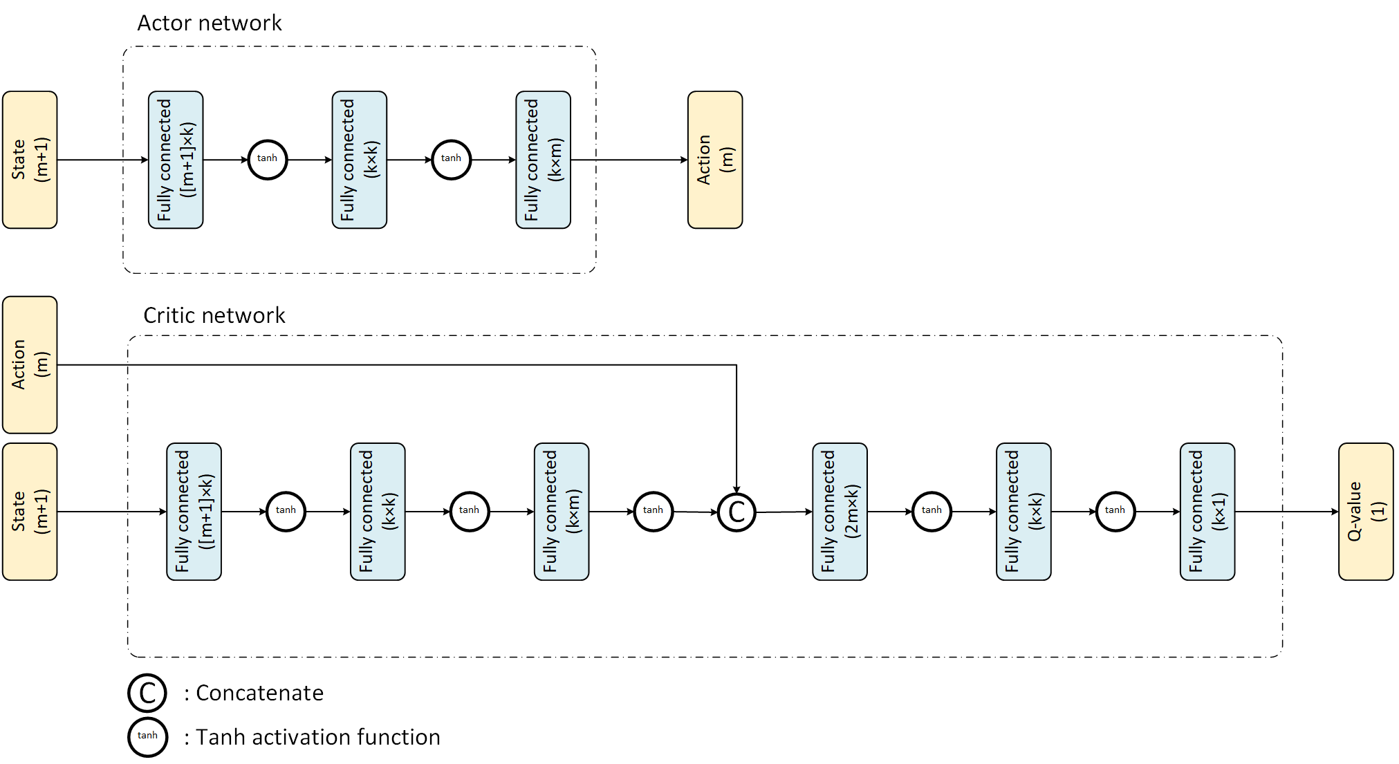
Our implementation of the ACRL algorithm involves two networks, one for the actor and one for the critic, both of which are presented in Figure 1. Since the numerical experiments assume that the underlying assets of the options follow a Brownian motion process, the model only needs to consider the most recent price for each asset to make investment decisions and the time to maturity. Consequently, the input state to each of the actor and critic networks includes the logarithm of each asset’s cumulative return, and the time remaining until maturity, which together correspond to an input vector of dimension $m+1$.

The actor network is composed of three fully connected layers where the number of neurons are considered to be $k=32$ in the first two layers and then maps back to the number of assets in the last layer so that the model generates the investment policy accordingly for each asset. The activation functions in our networks are considered to be tanh functions. In the last layer, this implies that the actions will lie in $[-1,\,1]^{m}$.

The critic network is operating on the same state information, while the $m$ dimensional action information vector is only concatenated to the output of the third layer. The first three layers of the critic network follow the same structure as the actor network in terms of the number of neurons, then after concatenating the action into the network, the two fully connected layers following the concatenation maps the number of neurons again to $k=32$. Finally, the last layer is a fully connected layer with one neuron to make sure that the output is a scalar representing the approximated Q value function.

Figure 1: The architecture of the actor and critic networks in ACRL algorithm.

4.2 ACRL training procedure for DRM and the role of translation invariance

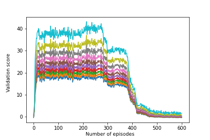
We now explain the training procedure employed for the actor and critic networks in the DRM. Recall that in an SRM setting, overfitting of any DRL algorithm can be controlled by measuring the performance of the trained policy on a validation data set using an empirical estimate of the risk-averse objective as validation score. Unfortunately, this is no longer possible in the case of DRMs since the risk measure relies on conditional risk measurements of the trajectories produced by our policy. In theory, estimates of such conditional measurements could be obtained by training a new critic network using the validation set (while maintaining the policy fixed to the trained one). In practice, this is highly computationally demanding to perform in the training stage and raises a new issue of how to control overfitting of the validation score estimate. Our solution for this problem is to rely on using a static risk measure as validation score. Given that it is unclear how to best replace a dynamic expectile risk measure with a static one, we choose to compute a set of validation scores that report the performance for a set of static expectiles at risk levels that are larger or equal to the risk level of the DRM. Relying on higher risk levels is motivated by the fact that dynamic expectile measures capture a more risk averse attitude than their static counterpart at the same risk level $\tau$. Figure 2(a) and (b) show examples of learning curves for the validation performance of a DRM when trained to hedge the writer and buyer positions of a vanilla option at a risk level of $\tau=90\%$. In this experiment, it appears that convergence roughly happens at all levels of $\tau\geq 90\%$. This approach is applied in all of our experiments for choosing the optimal number of episodes. We also note that both our training and validation sets included 1000 trajectories from the underlying geometric Brownian motion process. This implies that the training procedure used in these experiments can naturally extend to settings where only historical data is available.

(a) ACRL for DRM’s writer

(b) ACRL for DRM’s buyer

(c) AORL for SRM’s writer

(d) AORL for SRM’s buyer

Figure 2: Learning curves of the DRM and SRM for an at-the-money vanilla call option on APPL when a 90% expectile measure is used. The graphs show the validation scores for a range of static expectile measures with risk level ranging from $90\%$ to $99\%$.

We close this section with a short discussion about the role of the translation invariance property of dynamic risk measures. In particular, the work of Marzban et al. (2020) explains how without this property, the dynamic programming equations need to keep track of the wealth accumulated since $t=0$ using an additional state variable that gets only employed at $t=T$. More importantly, without translation invariance, the MDP representation ends up only having a reward at $t=T$ thus preventing the ACRL algorithm from receiving quick feedback about the quality of the actions that it is proposing. To illustrate the effect of this property, we compared the convergence of the training process for the ACRL algorithm under both form of DP representation of the buyer’s DRM. Namely, Figure 3 presents the learning curves of ACRL with immediate rewards as described in Section 3.2, while (b) presents the learning curves for an implementation in which all the rewards are delayed (using an additional state variable) until $t=T$. These figures clearly show that the MDP with immediate rewards is much easier to train than the delayed rewards MDP. In particular, not only does this model converge in less number of episodes, it also ends up converging to a better solution: the immediate rewards MDP converges to a risk of -0.59 for the buyer (0.91 for the writer), while with delayed rewards it converges to -0.41 (1.01).

(a) With immediate rewards

(b) With delayed rewards

Figure 3: Learning curves of the ACRL algorithm for the buyer’s DRM when using (a) the immediate rewards versus (b) delayed rewards in the hedging of a vanilla call at-the-money option.

4.3 Vanilla call option pricing and hedging

In our first set of experiments, we consider pricing and hedging an at-the-money vanilla call option on APPL. We should first note that solving a hedging problem, e.g. DRM, for a vanilla option is not particularly difficult since the number of state variables in this case is small. It is possible to obtain (approximately) optimal solutions by dynamic programming (Marzban et al. (2020)). Our purpose of considering the case of vanilla option is twofold. First, it provides a useful basis for checking the accuracy of solutions obtained from our deep reinforcement learning (DRL) methods against the ”true” optimal solutions, namely by comparing against the DP solutions. Such an accuracy check would be useful for justifying our use of DRL later in this paper as a general means to evaluate hedging performance and calculate the equal risk price (which becomes necessary for problems that cannot be solved by DP such as the case of basket options discussed in the next section). Second, the setting of a vanilla option also allows us to provide a more accurate comparison between DRM and SRM and demonstrate the advantage of the former, i.e. the benefit of time-consistent hedging policies, particularly when options with different time to maturity need to be considered.

To proceed, we first detail how the experiments are conducted. First, the initial price of the underlying stock APPL is always set to be 78.81, and the hedging portfolio is rebalanced on a monthly basis. Options with different time to maturity are considered, ranging from one month to one year. We generate from a Brownian motion three sets of price trajectories with one year time window, one for training, one for validation, and one for testing, and each consists of 1000 trajectories. In the training phase, we solve both DRM and SRM for the writer and buyer’s hedging problems using the longest maturity time, i.e. one year, as the hedging horizon. In solving the DRM, a policy and a critic network are trained using ACRL, whereas in solving the SRM, only a policy network is trained using AORL. See also Section 4.2 regarding how the validation is done to guide the training. Figure 2 presents the learning curves for the training of the hedging policies of the DRM and the SRM with a risk level of $\tau=90\%$. SRM appears to have a faster rate of convergence than DRM, which might not be surprising given that the architecture of SRM is simpler . It is however worth noting that the issue of time inconsistency for SRM implies that it can potentially produce poor quality policies and prices when the maturity of the option is modified unless it is completely retrained for each type of maturity. This is not the case for DRM and will be further discussed below.

With the trained DRM and SRM policy networks for a fixed 1 year maturity and risk aversion level $\tau\in\{75\%,90\%,95\%\}$, we can evaluate the writer and the buyer’s (out-of-sample) risk exposure over a pre-specified time horizon so as to calculate the corresponding ERP. We consider the following three metrics for measuring the realized risk under different hedging policy and explain the methods used for calculating the metrics:

• Out-of-sample static expectile risk: Given a trained policy network, use the testing data to calculate the static expectile risk obtained when hedging the option using this policy.

• RL based out-of-sample dynamic expectile risk estimation: Use the testing data to train only the critic network in ACRL for evaluating the out-of-sample dynamic risk. In particular, by fixing the policy network in ACRL to a trained policy network, the critic network trained based on testing data provides an estimate of the out-of-sample dynamic expectile risk. To speed up the training of the critic network, one may initialize the critic network using the network trained previously with the training data.

• DP based out-of-sample dynamic expectile risk estimation: Given a trained policy network, evaluate the “true” dynamic expectile risk by solving the dynamic programming equations, under the fixed policy, using a high precision discretization of the states, actions, and transitions. Note that this metric is available neither for the case of basket option nor in a data-driven environment where the stochastic process is unknown.

We note that our RL based estimate of out-of-sample dynamic risk is a novel concept, which refers to the calculation of dynamic risk based on testing data. This is possible, as explained above, by training only the critic network using ACRL on the test data. This metric is especially relevant given that classical methods for calculating dynamic risk, such as our DP based estimate, assume full knowledge of the stochastic model that captures the dynamics of an underlying system, i.e. stock price, and require the resolution of dynamic programming equations, which is known to suffer from the curse of dimensionality. Consequently, such methods can no longer be used when the DP equations require a large state space, as can be the case with basket options, or when the description of the underlying stochastic process is unknown.

In our experiments, we apply the second and third metric to the trained DRM policies and the first metric to both the trained DRM and SRM policies. In the former case, we are interested in demonstrating that the RL based out-of-sample expectile risk estimate is an accurate metric. Namely, we will compare the RL based estimate against the “true” DP based estimate. In the latter case, we will shed light on how the DRM policy performs when evaluated according to other metrics that are also of interest to practitioners. In particular, the static expectile risk measure, despite its issue of time inconsistency, can still have its intuitive appeal as a metric, and one may be interested in knowing how a DRM policy performs against this metric as compared to an SRM policy.

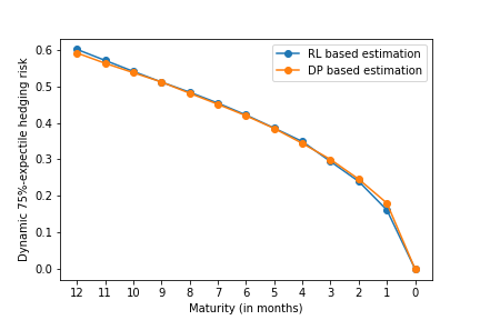
Figure 4 summarizes the evaluations of out-of-sample dynamic risk for DRM policies trained for 1 year maturity then applied to options of different maturities ranging from 12 months to 2 months. One can observe that the risk of the writer decreases monotonically for options of shorter maturities, whereas the risk of the buyer increases monotonically. This is consistent with the fact that there is less uncertainty for a shorter hedging horizon, which favors the writer’s risk exposure more than the buyer’s when considering an at-the-money option. This also provides the evidence that the DRM policies, albeit only trained based on the longest time to maturity, i.e. one year, can be well applied to hedge options with shorter time to maturity and be used to draw consistent conclusion. The observation that the DRM policies remain good policies for problems with shorter time to maturity testifies of the value of using a time consistent hedging model. Another important observation one can make is that the RL based out-of-sample dynamic risk estimate is generally very close to the DP based estimate across all conditions. The difference between the two appears to be more noticeable for the case of high risk aversion, i.e. $\tau=95\%$ and long time to maturity, but the difference remains minor overall. This observation allows us to confirm the accuracy of our RL based out-of-sample dynamic risk estimation procedure as a replacement for the DP based estimation in settings where the latter cannot be used.

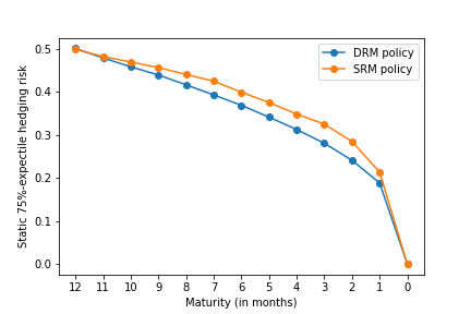
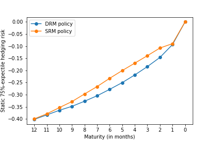
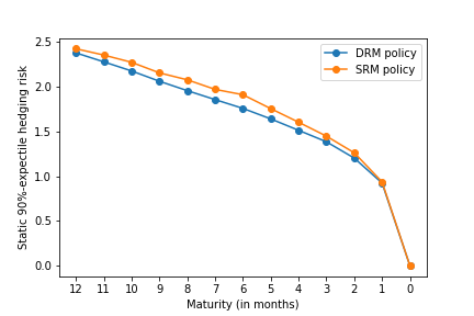
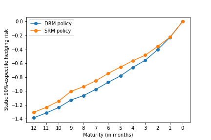
Figure 5 reports the out-of-sample static risk for both SRM policies and DRM policies. The results are interesting and perhaps surprising. First, unlike the consistent behavior observed in the case of dynamic risk, i.e. Figure 4, the static risk of SRM policies for the seller (resp. buyer) may increase (resp. decrease) when hedging an option with shorter maturity. The possibility that a seller’s policy may actually increase risk when applied to an option with shorter maturity is clearly problematic when the underlying asset follows a geometric brownian motion with positive drift, as it is inconsistent with the fact that there is less uncertainty (and lower expected value) regarding the payout of such options. This inconsistency occurs because the SRM policies are only trained based on the longest time to maturity, i.e. one year, and they cannot be well applied, unlike for the case of DRM policies, to problems with shorter time to maturity due to the violation of the time consistency property. It is clear from the figures that the SRM policies can be far from the optimal policies when applied to a shorter time to maturity. On the other hand, the DRM policies can actually be found not only to outperform SRM policies in terms of static risk exposure but also to generate consistent results across time, i.e. risk decreases (resp. increases) for the seller (resp. buyer) as the time to maturity decreases. This can be somewhat surprising, as the DRM policies are optimized based on dynamic risk measures rather than the static ones, but the policies can still perform well when evaluated according to static risk measures. Overall, the results presented in Figure 5 best showcase the strength of time consistent policies and why such policies are important to consider in settings where risk needs to be re-evaluated across different time points or maturity dates. We suspect that the possibility that SRM policies may not account properly for risk aversion at some future time point or for other range of option maturities should seriously hinder their use in practice.

In order to be more precise about results presented in figures 4 and 5, we detail in Table 3 all the numerical results for the case of high risk aversion, i.e. $\tau=90\%$ , along with the equal risk prices calculated based on RL based out-of-sample dynamic risk estimate and based on the discretized DP (referred as True ERP). One first confirm that the RL based estimateof ERP is a high quality approximation of the true ERP in this vanilla option pricing setting, with a maximum approximation error of 0.01 over all maturity dates. Moreover, we can see that the prices for the SRM polices are generally higher than the prices for the DRM polices. The observation is that while DRM policies are less risky than SRM policies across different time to maturity, it is the writer that benefits more from the use of DRM than the buyer. This could be related to the fact that the writer’s loss due to the option payout is unbounded while the option protects the buyer from losses. This in turns implies that the writer’s risk exposure is larger in this transaction. Thus, the choice of a policy can be more critical to the writer than the buyer. As the risk exposure of the writer decreases more than for the buyer, this leads to lower ERP price for DRM policies.

(a) Writer, $\tau=75\%$

(b) Buyer, $\tau=75\%$

(c) Writer, $\tau=90\%$

(d) Buyer, $\tau=90\%$

(e) Writer, $\tau=95\%$

(f) Buyer, $\tau=95\%$

Figure 4: The out-of-sample dynamic risk imposed to the two sides of a vanilla at-the-money call option over APPL (with maturity ranging from 12 months to 0 months) under the DRM policy trained for a 12 months maturity and at different risk levels $\tau\in\{75\%,90\%,95\%\}$.

(a) Writer, $\tau=75\%$

(b) Buyer, $\tau=75\%$

(c) Writer, $\tau=90\%$

(d) Buyer, $\tau=90\%$

(e) Writer, $\tau=95\%$

(f) Buyer, $\tau=95\%$

Figure 5: The out-of-sample static risk imposed to the two sides of a vanilla at-the-money call option over APPL (with maturity ranging from 12 months to 2 months) under the DRM and SRM policies trained for a 12 months maturity and at different risk levels $\tau\in\{75\%,90\%,95\%\}$.

Table 3: The out-of-sample dynamic and static 90%-expectile risk imposed to the two sides of vanilla at-the-money call options over APPL, with maturities ranging from 12 to 0 months, when hedged using the DRM and the SRM policies trained at risk level $\tau=90\%$ and for a 12 months maturity. Associated ERPs under the DRM are also compared to the “true” ERP measured using a discretized MDP.

		Time to maturity
Policy	Est.†	12	11	10	9	8	7	6	5	4	3	2	1
Dynamic 90%-expectile risk
Writer’s DRM	RL	0.77	0.73	0.69	0.65	0.62	0.58	0.53	0.48	0.45	0.38	0.29	0.23
	DP	0.75	0.71	0.68	0.65	0.61	0.57	0.53	0.49	0.43	0.38	0.31	0.23
Buyer’s DRM	RL	-0.22	-0.21	-0.20	-0.19	-0.18	-0.16	-0.15	-0.13	-0.11	-0.09	-0.07	-0.05
	DP	-0.23	-0.22	-0.21	-0.20	-0.18	-0.17	-0.16	-0.14	-0.12	-0.11	-0.08	-0.06
Static 90%-expectile risk
Writer’s SRM	ED	0.55	0.54	0.54	0.53	0.53	0.53	0.52	0.50	0.48	0.46	0.41	0.31
Writer’s DRM	ED	0.56	0.54	0.52	0.50	0.47	0.44	0.42	0.39	0.36	0.33	0.29	0.24
Buyer’s SRM	ED	-0.35	-0.33	-0.30	-0.27	-0.23	-0.20	-0.17	-0.13	-0.09	-0.07	-0.07	-0.06
Buyer’s SRM	ED	-0.36	-0.34	-0.32	-0.30	-0.28	-0.26	-0.24	-0.21	-0.18	-0.14	-0.11	-0.06
Equal risk prices with DRM
True ERP		0.49	0.47	0.45	0.42	0.40	0.37	0.34	0.31	0.28	0.24	0.19	0.14
DRM	RL	0.50	0.47	0.45	0.42	0.40	0.37	0.34	0.31	0.28	0.24	0.18	0.14
SRM	RL	0.49	0.46	0.44	0.43	0.40	0.38	0.35	0.33	0.30	0.27	0.24	0.22

^† Estimation (Est.) is either made based on reinforcement learning (RL), discretized dynamic programming (DP), or with the empirical distribution (ED).

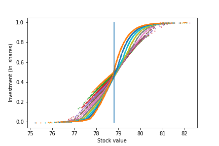
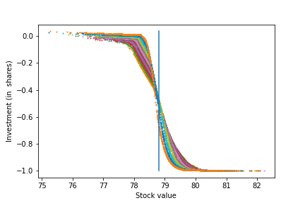
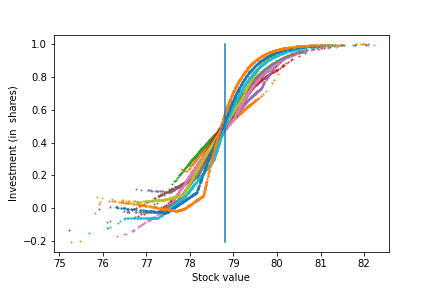
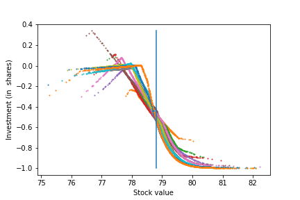
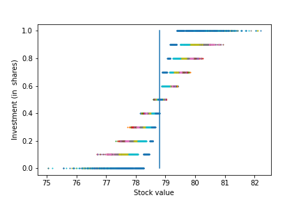
Finally, Figure 6 presents the optimal policies of the two models (i.e., DRM and SRM), together with the actual optimal policy of DRM, obtained using a high precision dynamic program (referred as DP-DRM). Each subfigure shows the policy as a function of current price ($x$-axis) and time period (colors). The figure further confirms that the policies of both DRM and SRM follow a similar pattern as DP-DRM, which ensures the quality of implementation of both AORL for SRM and ACRL for DRM.

(a) DRM’s writer

(b) DRM’s buyer

(c) SRM’s writer

(d) SRM’s buyer

(e) DP-DRM’s writer

(f) DP-DRM’s buyer

Figure 6: Comparison of the optimal DRL policies obtained for DRM and SRM (with 90% expectile measures) to the discretized DP solution (DP-DRM) for an at-the-money vanilla call option on APPL with a one year maturity. Each figure presents the sampled actions in our simulated trajectories as a function of the APPL stock value. The strike price is marked at 78.81.

4.4 Basket options

In our second set of experiments, we extend the application of ERP pricing framework to the case of basket options where traditionnal DP solution schemes are not computationally tractable. In particular, we consider an at-the-money basket option with the strike price of $753\$$ on five underlying assets: APPL, AMZN, FB, JPM, and GOOGL, where the option payoff is determined by the average price of the underlyings. Similarly to the case of the vanilla option, the rebalancing of the portfolio is happening once per month, options with different maturities from one month to twelve months are considered, and three sets of price trajectories are used for training, validation, and testing the models. We train the ACRL and AORL networks for a one year basket option and then use the same policy network for hedging options with shorter time to maturity.

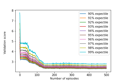
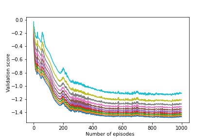
Our first observation in this set of experiments relates to the training time of the model for the basket option with five assets. Figure 7 presents the convergence of the training of the ACRL model under $\tau=90\%$. When comparing to the case of the vanilla option, the convergence rate appears to have a similar behavior, i.e., the number of episodes and the time spent on each episode is similar for both the case of the writer and the buyer. This is important as it indicates that the training time might not be very sensitive to the number of assets, while traditional DP approaches are known to become intractable when the option is written on multiple assets.

In this section, dynamic risk is estimated using the RL based estimator described in Section 4.3 given that the DP estimator requires too much computations and that the RL based one was shown to provide a relatively high precision estimation of the “true” dynamic risk. Following this, in Figure 8 (a) and (b) we present the dynamic risk obtained from applying the DRM policy on the test data when the model is trained for a one year maturity option. Hedging risk using the same trained policy is presented for 12 different options with maturity ranging from 0 to 12 months. Similar to the vanilla option case, the dynamic risk of the writer is monotonically decreasing as we get closer to the maturity of the option, which can be attributed to the reduced probability that the average price of the assets significantly diverges from the initial average (i.e., the strike price of the option). On the other side, i.e. for the buyer of the option, although overall the risk is increasing to zero as the maturity gets closer to zero, for longer time to maturities we observe some degradation of risk. We attribute this behavior to the estimation error of the RL based dynamic risk estimator.

In order to have a view of risk that is not perturbed by estimation errors, we also compare the static risk under DRM and SRM as we did for vanilla options. Figure 9 (a) and (b) shows the static risk under $\tau=90\%$. One can first recognize the same monotone convergence to zero of the two sides of the options. However, contrary to the case of the vanilla option, the difference between the static risk performance of DRM and SRM policies are rather similar for all maturity times. It therefore appears that in these experiments with a basket option, both SRM and DRM produce similar polices. One possible reason could be that the range of “optimal” risk averse investment plans, whether using DRM or SRM, is more limited. Indeed, while for the vanilla option, we observed that the optimal policies generated investments in the range [0, 1] and [-1, 0] for the writer and the buyer respectively, for the basket option we observed wealth allocations that are more concentrated around 0.20 (i.e. the uniform portfolio known for its risk hedging properties) and -0.20 for each of the 5 assets asset respectively. Finally, similar to the vanilla option case, Table 4 presents more details on the results used to produce figures 8 and 9, along with the equal risk prices computed based on our RL based out-of-sample dynamic risk estimator. The higher ERP price for the SRM policy is an obvious observation in this table, which again can be attributed to the better performing (in terms of dynamic risk) hedging policy produced by ACRL for the DRM, compared to the policy produced by AORL for the SRM.

(a) Writer

(b) Buyer

Figure 7: Learning curves of the ACRL algorithm for the writer and buyer’s DRM for a basket at-the-money call option over APPL, AMZN, FB, JPM, and GOOGL at the risk level $\tau=90\%$. The graphs show the validation scores for a range of static expectile measures with risk level ranging from $90\%$ to $99\%$.

(a) Writer

(b) Buyer

Figure 8: The out-of-sample dynamic risk imposed to the two sides of a basket at-the-money call option over APPL, AMZN, FB, JPM, and GOOGL at the risk level $\tau=90\%$ (as maturity ranges from 12 to 0 months) under a DRM policy trained for a 12 months maturity.

(a) Static risk, writer

(b) Static risk, buyer

Figure 9: The out-of-sample static risk imposed to the two sides of a basket at-the-money call option over APPL, AMZN, FB, JPM, and GOOGL at the risk level $\tau=90\%$ (as maturity ranges from 12 to 0 months) under the DRM and SRM policies trained for a 12 months maturity.

Table 4: The out-of-sample dynamic and static 90%-expectile risk imposed to the two sides of basket at-the-money call options over APPL, AMZN, FB, JPM, and GOOGL, with maturities ranging from 12 to 0 months, when hedged using the DRM and the SRM policies trained at risk level $\tau=90\%$ and for a 12 month maturity. Associated ERPs under the DRM are also compared.

		Time to maturity
Policy	Est.†	12	11	10	9	8	7	6	5	4	3	2	1
Dynamic 90%-expectile risk
Writer’s DRM	RL	3.92	3.62	3.38	3.15	2.95	2.72	2.48	2.25	2.00	1.70	1.39	1.10
Buyer’s DRM	RL	-0.48	-0.49	-0.51	-0.52	-0.50	-0.49	-0.48	-0.48	-0.47	-0.37	-0.33	-0.29
Static 90%-expectile risk
Writer’s SRM	ED	2.43	2.36	2.28	2.16	2.08	1.97	1.91	1.76	1.61	1.45	1.26	0.94
Writer’s DRM	ED	2.38	2.28	2.18	2.06	1.96	1.86	1.76	1.64	1.51	1.39	1.20	0.92
Buyer’s SRM	ED	-1.31	-1.24	-1.15	-1.01	-0.94	-0.85	-0.75	-0.66	-0.56	-0.48	-0.36	-0.22
Buyer’s SRM	ED	-1.39	-1.32	-1.24	-1.13	-1.07	-0.98	-0.88	-0.78	-0.66	-0.56	-0.40	-0.23
Equal risk prices with DRM
DRM	RL	2.20	2.06	1.95	1.84	1.73	1.61	1.48	1.37	1.24	1.04	0.86	0.70
SRM	RL	2.23	2.10	2.01	1.91	1.79	1.65	1.52	1.39	1.21	1.03	0.92	0.82

^† Estimation (Est.) is either made based on reinforcement learning (RL), discretized dynamic programming (DP), or with the empirical distribution (ED).

5 Conclusion

In this paper, we developed and implemented the first deep reinforcement learning algorithm for calculating equal risk prices under time consistent dynamic risk measures. This algorithm exploits the elicitability property of the expectile risk measure to extend in a natural way the famous off-policy deterministic actor-critic method presented in Silver et al. (2014) to the risk averse setting. Our numerical experiments confirmed that it can identify risk averse hedging strategies of good quality and be used to estimate the ERP, simultaneously for a range of maturities, using a reasonable amount of computational resources in conditions where traditional DP methods are impracticable. We also demonstrated important issues regarding the implementability of hedging strategies that are based on static (time inconsistent) risk measures. Namely, both our illustrative example and two numerical experiments demonstrated how the time consistent policy produced using the DRM might in fact appear preferable to the investor (from the point of view of the time inconsistent static risk measure) as the risk is measured at later points of time, i.e. with shorter maturity. Overall, as the first paper that is considering option pricing under ERP using time consistent dynamic risk measures, we only evaluated the performance of our model in a synthetic environment using a simple neural network architecture. One may be interested in examining the performance of this model under real market conditions. In particular, in a simulation environment having access to infinite i.i.d. samples makes training much easier to machine learning models. In a real market environment, where the available data is limited to some non-stationary samples of past historical prices, training an on-policy network will face serious issues associated to lack of exploration. This might result in even higher out performance of the ACRL model compared to the AORL, and therefore superior hedging precision under the time consistent dynamic risk measure. In addition, we only consider European style options in this paper, where as demonstrated in Marzban et al. (2020), the ERP model can also be investigated in the case of American options.

References

- Guo and Zhu (2017) Ivan Guo and Song-Ping Zhu. Equal risk pricing under convex trading constraints. Journal of Economic Dynamics and Control, 76:136–151, 2017.
- Marzban et al. (2020) Saeed Marzban, Erick Delage, and Jonathan Yumeng Li. Equal risk pricing and hedging of financial derivatives with convex risk measures. arXiv preprint arXiv:2002.02876, 2020.
- Carbonneau and Godin (2020) Alexandre Carbonneau and Frédéric Godin. Equal risk pricing of derivatives with deep hedging. Quantitative Finance, pages 1–16, 2020.
- Carbonneau and Godin (2021) Alexandre Carbonneau and Frédéric Godin. Deep equal risk pricing of financial derivatives with multiple hedging instruments. arXiv preprint arXiv:2102.12694, 2021.
- Williams (1992) Ronald J Williams. Simple statistical gradient-following algorithms for connectionist reinforcement learning. Machine learning, 8(3):229–256, 1992.
- Mnih et al. (2015) Volodymyr Mnih, Koray Kavukcuoglu, David Silver, Andrei A Rusu, Joel Veness, Marc G Bellemare, Alex Graves, Martin Riedmiller, Andreas K Fidjeland, Georg Ostrovski, et al. Human-level control through deep reinforcement learning. Nature, 518(7540):529–533, 2015.
- Silver et al. (2014) David Silver, Guy Lever, Nicolas Heess, Thomas Degris, Daan Wierstra, and Martin Riedmiller. Deterministic policy gradient algorithms. In International conference on machine learning, pages 387–395. PMLR, 2014.
- Tamar et al. (2015) Aviv Tamar, Yinlam Chow, Mohammad Ghavamzadeh, and Shie Mannor. Policy gradient for coherent risk measures. In C. Cortes, N. Lawrence, D. Lee, M. Sugiyama, and R. Garnett, editors, Advances in Neural Information Processing Systems, volume 28. Curran Associates, Inc., 2015.
- Huang et al. (2021) Audrey Huang, Liu Leqi, Zachary C. Lipton, and Kamyar Azizzadenesheli. On the convergence and optimality of policy gradient for markov coherent risk, 2021.
- Bertsimas et al. (2001) Dimitris Bertsimas, Leonid Kogan, and Andrew W Lo. Hedging derivative securities and incomplete markets: an -arbitrage approach. Operations research, 49(3):372–397, 2001.
- Artzner et al. (1999) Philippe Artzner, Freddy Delbaen, Jean-Marc Eber, and David Heath. Coherent measures of risk. Mathematical finance, 9(3):203–228, 1999.
- Rudloff et al. (2014) Birgit Rudloff, Alexandre Street, and Davi M Valladão. Time consistency and risk averse dynamic decision models: Definition, interpretation and practical consequences. European Journal of Operational Research, 234(3):743–750, 2014.
- Bellini and Bignozzi (2015) Fabio Bellini and Valeria Bignozzi. On elicitable risk measures. Quantitative Finance, 15(5):725–733, 2015.
- Chen (2018) James Ming Chen. On exactitude in financial regulation: Value-at-risk, expected shortfall, and expectiles. Risks, 6(2):61, 2018.
- Bellini and Bernardino (2017) Fabio Bellini and Elena Di Bernardino. Risk management with expectiles. The European Journal of Finance, 23(6):487–506, 2017.
- Degris et al. (2012) Thomas Degris, Martha White, and Richard S. Sutton. Off-policy actor-critic. In Proceedings of the 29th International Coference on International Conference on Machine Learning, ICML’12, page 179–186, Madison, WI, USA, 2012. Omnipress.
- Shen et al. (2014) Yun Shen, Michael J. Tobia, Tobias Sommer, and Klaus Obermayer. Risk-sensitive reinforcement learning. Neural Computation, 26(7):1298–1328, 2014.
- Lillicrap et al. (2015) Timothy P Lillicrap, Jonathan J Hunt, Alexander Pritzel, Nicolas Heess, Tom Erez, Yuval Tassa, David Silver, and Daan Wierstra. Continuous control with deep reinforcement learning. arXiv preprint arXiv:1509.02971, 2015.
- Castro et al. (2019) Dotan Di Castro, J. Oren, and Shie Mannor. Practical risk measures in reinforcement learning. ArXiv, abs/1908.08379, 2019.
- Singh et al. (2020) Rahul Singh, Qinsheng Zhang, and Yongxin Chen. Improving robustness via risk averse distributional reinforcement learning. In Alexandre M. Bayen, Ali Jadbabaie, George Pappas, Pablo A. Parrilo, Benjamin Recht, Claire Tomlin, and Melanie Zeilinger, editors, Proceedings of the 2nd Conference on Learning for Dynamics and Control, volume 120 of Proceedings of Machine Learning Research, pages 958–968, 2020.
- Urpí et al. (2021) Núria Armengol Urpí, Sebastian Curi, and Andreas Krause. Risk-averse offline reinforcement learning. In ICLR 2021: The Ninth International Conference on Learning Representations, 2021.