First extragalactic measurement of the turbulence driving parameter: ALMA observations of the star-forming region N159E in the Large Magellanic Cloud

Abstract

Studying the driving modes of turbulence is important for characterizing the impact of turbulence in various astrophysical environments. The driving mode of turbulence is parameterized by $b$, which relates the width of the gas density PDF to the turbulent Mach number; $b\approx 1/3$, $1$, and $0.4$ correspond to driving that is solenoidal, compressive, and a natural mixture of the two, respectively. In this work, we use high-resolution (sub-pc) ALMA ¹²CO ($J$ = 2–1), ¹³CO ($J$ = 2–1), and C¹⁸O ($J$ = 2–1) observations of filamentary molecular clouds in the star-forming region N159E (the Papillon Nebula) in the Large Magellanic Cloud (LMC) to provide the first measurement of turbulence driving parameter in an extragalactic region. We use a non-local thermodynamic equilibrium (NLTE) analysis of the CO isotopologues to construct a gas density PDF, which we find to be largely log-normal in shape with some intermittent features indicating deviations from lognormality. We find that the width of the log-normal part of the density PDF is comparable to the supersonic turbulent Mach number, resulting in $b\approx 0.9$. This implies that the driving mode of turbulence in N159E is primarily compressive. We speculate that the compressive turbulence could have been powered by gravo-turbulent fragmentation of the molecular gas, or due to compression powered by H $I$1.2ex  flows that led to the development of the molecular filaments observed by ALMA in the region. Our analysis can be easily applied to study the nature of turbulence driving in resolved star-forming regions in the local as well as the high-redshift Universe.

1 Introduction

Turbulence is ubiquitous in the Universe and plays an important role in most astrophysical environments, from stellar interiors (Miesch & Toomre, 2009) to galaxy clusters (Zhuravleva et al., 2014). In many such environments, the impact of turbulence on the evolution of the gas is very complex (Burkhart et al., 2020). In particular, several works have shown how turbulence non-linearly impacts the physics of star formation (see recent reviews by Rosen et al., 2020; Girichidis et al., 2020). A classic example is that turbulence can either assist or hinder star formation in the interstellar medium (ISM) that can lead to an order of magnitude difference in star formation rates depending on the turbulence driving source (Federrath & Klessen, 2012; Salim et al., 2015). This is because the driving mode of turbulence influences the dynamics of the star-forming gas: if the turbulence is primarily composed of compressive (curl-free) modes, it will aid the compression of the gas, thus leading to the formation of dense cores. On the other hand, if the turbulence is primarily composed of solenoidal (divergence-free) modes, gas compression is significantly reduced compared to compressive driving (Federrath et al., 2008, 2010). The driving mode of turbulence sets the density and velocity fluctuations in star-forming molecular clouds, which in turn control collapse and fragmentation (Krumholz & McKee, 2005; Federrath & Klessen, 2012, 2013; Kainulainen et al., 2013; Burkhart et al., 2015; Kainulainen & Federrath, 2017). It also influences the chemistry and thermodynamics as the clouds collapse (Struck & Smith, 1999; Pan & Padoan, 2009; Immer et al., 2016; Sharda et al., 2019b, 2020; Sharda et al., 2021; Mandal et al., 2020). Thus, characterizing the mode of turbulence is critical to further our understanding of the lifecycle of molecular clouds.

There has been immense progress towards characterizing the driving mode of turbulence in the ISM, both in theory and simulations (e.g., Federrath et al., 2010; Pan et al., 2016; Jin et al., 2017; Körtgen et al., 2017; Mandal et al., 2020; Menon et al., 2020; Lim et al., 2020). In the absence of magnetic fields and assuming an isothermal equation of state, the mode of turbulence is typically defined as the ratio of the width of the normalized gas density probability distribution function (assumed to be log-normal), $\sigma_{\rho/\rho_{0}}$, to the turbulent Mach number, $\mathcal{M}$ (Padoan et al., 1997a; Passot & Vázquez-Semadeni, 1998)

$$b=\frac{\sigma_{\rho/\rho_{0}}}{\mathcal{M}}\,.$$ (1)

Simulations find that fully solenoidal driving of the turbulence produces $b\approx 1/3$, fully compressive driving produces $b\approx 1$, and a natural (steady-state) mixture of the two yields $b\approx 0.4$ (Federrath et al., 2010; Federrath et al., 2011). The physical origin of this relationship is simple: a driving field that contains primarily compressive modes produces stronger compressions and rarefactions, and thus results in a higher spread in the density probability distribution function (PDF) than a primarily solenoidal velocity field (see, for instance, Federrath et al., 2008; Burkhart & Lazarian, 2012; Beattie et al., 2021b). Examples of driving mechanisms that are largely compressive include hydrodynamical shocks, spiral waves, ionizing feedback from massive stars (Federrath et al., 2017; Menon et al., 2020; Beattie et al., 2021b). On the other hand, solenoidal turbulence is believed to be driven by magnetorotational instabilities (MRI) in accretion discs, protostellar outflows and stellar winds, and shearing motions, such as those induced by differential rotation (Hansen et al., 2012; Offner & Arce, 2014; Federrath et al., 2016; Offner & Chaban, 2017; Offner & Liu, 2018). It is also important to note that if strong magnetic fields are present, then $\mathcal{M}\to\mathcal{M}(1+1/\beta)^{-1/2}$ in equation 1. Here, $\beta$ is the turbulent plasma beta (e.g., Federrath & Klessen, 2012) that describes the strength of thermal to magnetic pressure: $\beta=2\mathcal{M}^{2}_{\rm{A}}/\mathcal{M}^{2}$, where $\mathcal{M}_{\rm{A}}$ is the Alfvén Mach number. The driving mode can also vary from between solenoidal and compressive both in time and space as the molecular clouds evolve (Körtgen et al., 2017; Orkisz et al., 2017; Körtgen, 2020). Thus, $b$ is best conceived as representing the instantaneous driving mode of turbulence in a system.

Despite great progress in measuring the driving mode of turbulence in simulations, it has only been investigated in a very limited sample of observations (Padoan et al. 1997b; Brunt 2010; Ginsburg et al. 2013; Federrath et al. 2016; Kainulainen & Federrath 2017; Marchal & Miville-Deschênes 2021; Menon et al. 2021; hereafter, M21), all of which remain limited to the Milky Way. This is because measuring $b$ requires constructing the gas density PDF, which needs either dust observations spanning a wide range of frequencies and extinctions (e.g., Schneider et al., 2013, 2015a), or multiple, optically-thin gas density tracers for gas at different densities (e.g., M21, ). Moreover, measuring $b$ also requires high spatial resolution from which reliable gas kinematics can be obtained (e.g., Sharda et al., 2018). These issues have so far prevented us from measuring the driving mode of turbulence in extragalactic observations.

In this paper, we provide the first observational measurement of the driving mode of turbulence in an extragalactic region. We utilize Atacama Large Millimeter/Submillimeter Array (ALMA) observations of the star-forming region N159E in the Large Magellanic Cloud (LMC) that contains the Papillon Nebula (Fukui et al., 2019, hereafter, F19). Located southwest of the core of the starburst region 30 Doradus, N159E lies at the eastern end of the star-forming giant molecular cloud (GMC) N159 (Johansson et al., 1994; Fukui et al., 2008; Minamidani et al., 2008; Chen et al., 2010). The exquisite resolution provided by ALMA has enabled spatially-resolved molecular gas studies of different parts of N159 on sub-pc scales in great detail (e.g., Fukui et al., 2015; Saigo et al., 2017; Nayak et al., 2018; Tokuda et al., 2019). Since the discovery of the first extragalactic protostar in the region (Gatley et al., 1981), further observations have revealed that N159 hosts a number of massive young stellar objects (YSOs; Heydari-Malayeri et al., 1999; Indebetouw et al., 2004; Meynadier et al., 2004; Nakajima et al., 2005; Testor et al., 2006, 2007; Seale et al., 2009; Chen et al., 2010; Saigo et al., 2017; Nayak et al., 2018; Galametz et al., 2020), making it an ideal region to study the turbulence in molecular clouds impacted by protostellar feedback. In this work, we measure the mode of turbulence in the filamentary structure comprised of molecular gas, including outflows from two newly-identified dense cores that are suspected to harbour massive, young ($<10^{4}\,\mathrm{yr}$) protostars in N159E (F19).

We arrange the rest of this paper as follows: Section 2 describes the ALMA data we use in this work, Section 3 describes how we measure the gas density PDF and the turbulent Mach number, Section 4 presents our results, Section 5 lays out the caveats for our work, and Section 6 discusses the possible drivers of turbulence in N159E. Finally, we present our conclusions in Section 7. For this work, we assume the metallicity of the LMC to be $0.5\,\rm{Z_{\odot}}$ (e.g., Hughes et al., 1998; Schenck et al., 2016), and distance to the LMC to be $50\,\mathrm{kpc}$ (e.g., Pietrzyński et al., 2019), corresponding to 0$\aas@@fstack{\prime\prime}$1 $=0.24\,\mathrm{pc}$.

2 Data

N159E was observed during Cycle 4 using ALMA Band 6 (P.I. Y. Fukui, #2016.1.01173.S.), targeting multiple molecular lines – ¹²CO $(J=2-1)$, ¹³CO $(J=2-1)$, C¹⁸O $(J=2-1)$, and SiO $(J=5-4)$, as well as the $1.3\,\rm{mm}$ continuum. We refer the readers to F19 and Tokuda et al. (2019) for details on the data reduction and analysis of these ALMA observations; here, we note the main features that are relevant to this work. The beam size of these observations is 0.28″$\times$ 0.25″(for the CO isotopologues) and 0.26″$\times$ 0.23″(for the $1.3\,\rm{mm}$ continuum), corresponding to a spatial resolution of $\sim 0.07\,\rm{pc}$. The observations detected significant flux in all three CO lines, at an rms noise level of $\sigma_{{}^{12}\rm{CO}}\sim 4\,\rm{mJy\,beam^{-1}}$ for ¹²CO, $\sigma_{{}^{13}\rm{CO}}\sim 4.5\,\rm{mJy\,beam^{-1}}$ for ¹³CO, and $\sigma_{\rm{C^{18}O}}\sim 4.5\,\rm{mJy\,beam^{-1}}$ for C¹⁸O. These observations also revealed detailed, filamentary structures comprised of molecular gas that were unresolved in previous Cycle 1 ALMA observations of N159E at lower resolution ($\sim 0.24\,\rm{pc}$, Saigo et al. 2017). We do not utilize the Cycle 1 data as the Cycle 4 data shows no significant missing flux at higher resolution (F19).

Figure 1 shows the integrated intensity (moment 0) map of ¹³CO in N159E as imaged by ALMA (see also, figure 1 of F19). The Papillon Nebula YSO binary system (masses $\sim 21\,\rm{M_{\odot}}$ and $41\,\rm{M_{\odot}}$ – Heydari-Malayeri et al. 1999; Indebetouw et al. 2004; Testor et al. 2007; Chen et al. 2010) lie towards the southern half of the region, marked by the magenta box. The black box encloses the $\sim 1\times 4\,\rm{pc}$ region we analyze in this work (hereafter, referred to as the ‘analysis region’). It possibly consists of filamentary molecular gas structures (see figure 4 of F19) that trace a larger-scale H $I$1.2ex  gas distribution (Fukui et al., 2017), and two other compact sources called MMS-1 and MMS-2 identified by F19. These compact sources are most likely massive YSOs believed to have formed as a result of colliding flows (F19; Fukui et al. 2021), which are responsible for driving outflows within the region. The outflowing gas spans $\sim 30\,\rm{km\,s^{-1}}$ in velocity. Note that we cannot put constraints on the actual size of the outflows (although they are believed to be $0.1\,\rm{pc}$ long), or distinguish between the outflowing gas from one massive YSO to the other. Thus, our analysis region consists of a mixture of filamentary molecular clouds where massive YSOs driving outflows are present. We cannot exclude a part of the contiguous structure in this region because a sufficiently large field of view is necessary to properly sample the low column density part of the PDF (Körtgen et al., 2019), as well as to retrieve reliable gas kinematics from the data (Sharda et al., 2018).

3 Analysis

Below we describe the general method we adopt to derive the column density and velocity structure of molecular gas in the region, construct their PDFs, and calculate their respective density and velocity dispersions.

3.1 Gas density PDF

We use the three CO isotopologues to construct the gas density PDF. We also assume the following abundance ratios for N159E: $X[\rm{H_{2}}/^{12}\mathrm{CO}]=62500$ (Fukui et al., 2008), $X[^{12}\mathrm{CO}/^{13}\mathrm{CO}]=50$ (Mizuno et al. 2010; F19), and $X[^{12}\mathrm{CO}/\mathrm{C^{18}O}]=560$ (Wang et al., 2009), and we discuss the effects of varying these abundance ratios later in Section 5. Below, we first estimate the column density while assuming the gas to be in local thermodynamic equilibrium (LTE), as is commonly done in such analyses (e.g., M21, ). Then, we relax this assumption and perform a non-LTE (NLTE) analysis to derive the gas density PDF, showing how sub-thermal excitation of ¹³CO, in particular, can give rise to important deviations from an LTE approach for star-forming molecular clouds.

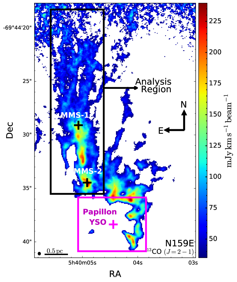
Figure 1: ALMA ¹³CO ($J$ = 2–1) integrated intensity map of N159E in the LMC. The magenta box marks the approximate extent of the Papillon Nebula that harbours the Papillon YSO binary system marked by the magenta cross. The $1\times 4\,\rm{pc}$ analysis region we use to measure the driving mode of turbulence is denoted by the solid, black box. This region contains two young, dense cores marked by the black crosses (MMS-1 and MMS-2, as identified by F19) that are suspected to contain massive YSOs that are driving $\sim 0.1\,\rm{pc}$ sized outflows in this region. The beam size (angular resolution $\approx 0.28\arcsec\times 0.25\arcsec$) is represented by the black circle in the bottom left corner, and the adjacent scale shows the physical extent of the region. The noisiness in the pixels towards the North is caused by the drop in sensitivity at the edge of the mosaic.

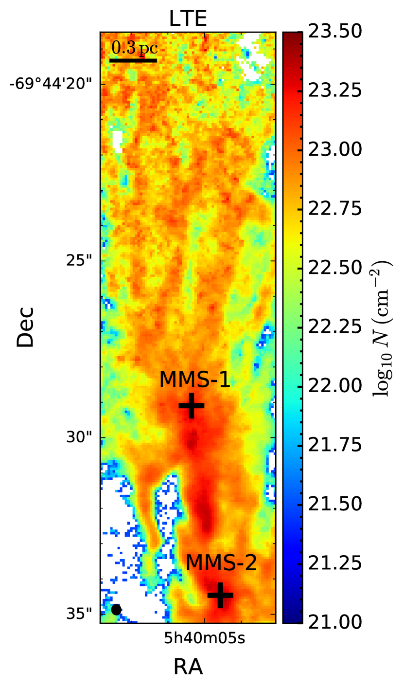
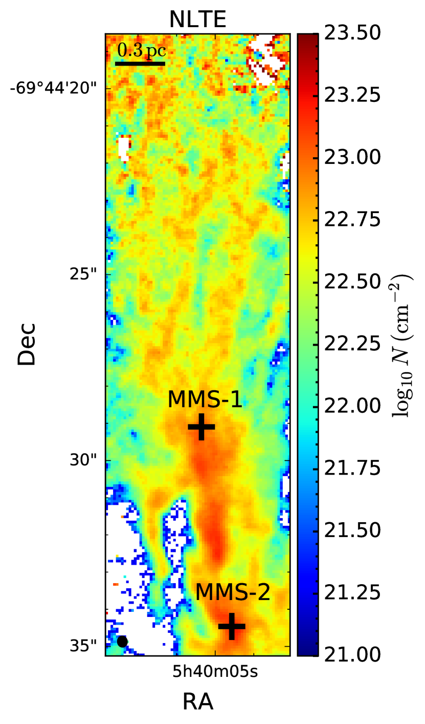
Figure 2: H₂ column density map of the analysis region shown in Figure 1, created using the ¹²CO ($J$ = 2–1), ¹³CO ($J$ = 2–1), and C¹⁸O ($J$ = 2–1) ALMA observations. The left panel shows the resulting column density when assuming CO isotopologues to be in local thermodynamic equilibrium (LTE) whereas the right panel shows the map for a non-LTE (NLTE) analysis. The beam size and scale are denoted in the bottom left and the top left corner of the plot, respectively. Black crosses denote the probable positions of the two massive, young protostars (MMS-1 and MMS-2) that are driving outflows in this region (F19).

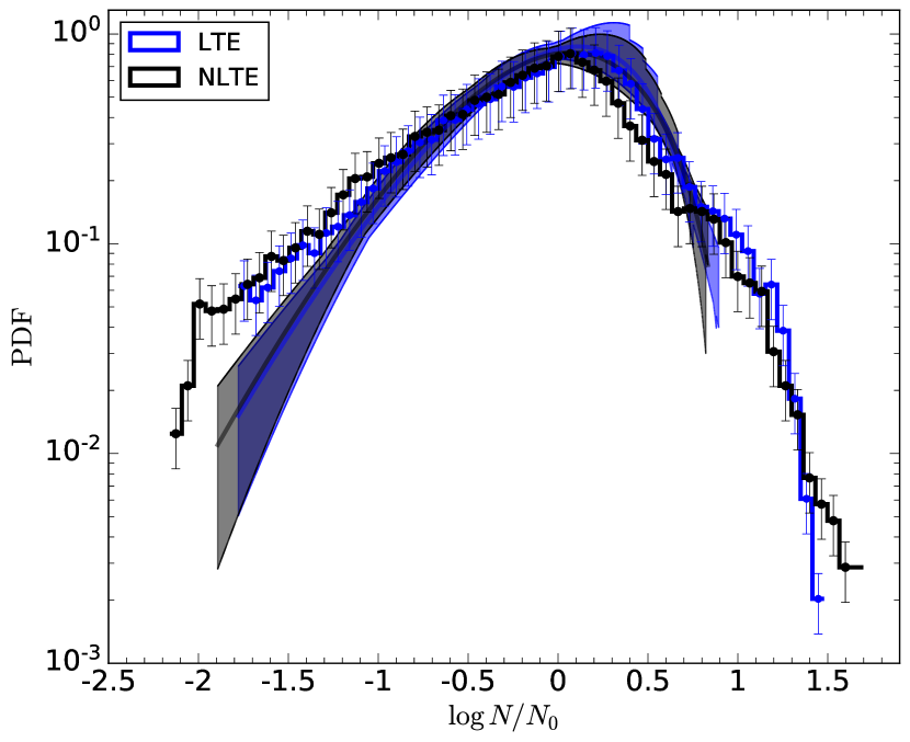
Figure 3: Normalized 2D column density PDF (with $1\sigma$ errors) of the analysis region shown in Figure 2, using the LTE and the NLTE methods described in Section 3.1. $N_{0}$ represents the mean column density. The distribution is largely log-normal, with some intermittent features indicating deviations from non lognormality. Fitting the Hopkins (2013) gas density PDF model (solid lines represent the best fit and shaded curves represent the $1\sigma$ error on the best fit) gives the 2D column density dispersion in the LTE case $\sigma_{N/N_{0}}\rm{(LTE)}=0.58\pm 0.14$, and in the NLTE case $\sigma_{N/N_{0}}\rm{(NLTE)}=0.51\pm 0.04$. The corresponding intermittencies are $\theta=0.12\pm 0.05$ (LTE) and $\theta=0.17\pm 0.09$ (NLTE). We use these 2D column density dispersions to derive the 3D density dispersion $\sigma_{\rho/\rho_{0}}$, following Brunt et al. (2010a).

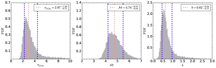
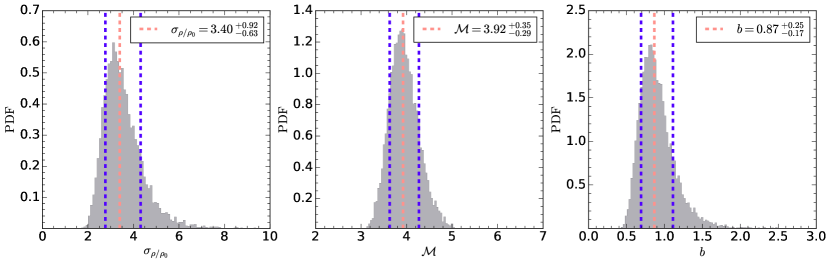
Figure 4: PDFs of the distributions of the 3D density dispersion ($\sigma_{\rho/\rho_{0}}$), turbulent Mach number ($\mathcal{M}$), and the driving mode of turbulence ($b$) obtained from 10,000 bootstrapping realisations. The top and the bottom row corresponds to the LTE and the NLTE analyses, respectively. The dashed orange line denotes the $50^{\rm{th}}$ percentile, whereas the dashed blue lines denote the $16^{\rm{th}}$ and the $84^{\rm{th}}$ percentiles, respectively.

3.1.1 LTE analysis

To trace the $\mathrm{H}_{2}$ gas column density structure under the LTE approximation, we follow M21 and use a hybrid method with a combination of the ¹³CO and C¹⁸O ($J$ = 2–1) lines. We do not use the ${}^{12}\mathrm{CO}$ emission to directly trace the $\mathrm{H}_{2}$ column density in this work, primarily because we expect ${}^{12}\mathrm{CO}$ to be optically thick in most of the analysis region, so it cannot accurately trace the true column density of $\mathrm{H}_{2}$ (however, see Mangum & Shirley, 2015, for an alternative method with a correction factor for optically-thick lines). In the hybrid method, we use C¹⁸O emission to trace the densest parts of the region where ¹³CO becomes optically thick, otherwise we use the ¹³CO emission. We estimate the optical depth of ¹³CO as $\tau_{13}=\tau_{12}X[^{13}\mathrm{CO}/^{12}\mathrm{CO}]$, where $\tau_{12}$ is the optical depth of ${}^{12}\mathrm{CO}$ that we calculate using the line ratio ${}^{\rm{iso}}R_{2}$ (¹²CO ($J$ = 2–1) to ¹³CO ($J$ = 2–1)) following equation 1 of Choi et al. (1993). Thus, we can determine from this relation whether ${}^{13}\mathrm{CO}$ is optically thick (i.e., $\tau_{13}>1$) in a given spectral channel and spatial region, in which case we use $\mathrm{C}^{18}\mathrm{O}$ to trace the $\mathrm{H}_{2}$ column density. We find that the maximum optical depths in the analysis region are such that C¹⁸O is never measured to become optically thick.

We then obtain the H₂ column density contribution for each pixel (with more than $3\sigma_{\rm{{}^{13}CO}}$ emission) from the main-beam brightness temperature $T_{\mathrm{MB}}$ of the relevant line as

$$N_{\mathrm{H}_{2}}=X[\mathrm{H}_{2}]\int f(T_{\mathrm{ex}})T_{\mathrm{MB}}\,dv,$$ (2)

where $X[\mathrm{H}_{2}]$ is the abundance factor used to convert the line column density to a H₂ column density, and $f(T_{\mathrm{ex}})$ is a function of the excitation temperature ($T_{\mathrm{ex}}$). The abundance factor is given by $X[\mathrm{H}_{2}]=X[^{12}\mathrm{CO}/^{13}\mathrm{CO}]\,X[\mathrm{H}_{2}/^{12}\mathrm{CO}]$ and $X[^{12}\mathrm{CO}/\mathrm{C}^{18}\mathrm{O}]\,X[\mathrm{H}_{2}/^{12}\mathrm{CO}]$ for ${}^{13}\mathrm{CO}$ and $\mathrm{C}^{18}\mathrm{O}$, respectively. The function $f$ is given by (Mangum & Shirley, 2015)

$$f\left(T_{\mathrm{ex}}\right)=\frac{3hZ}{8\pi^{3}\mu^{2}J_{u}}\frac{\exp\left(\frac{E_{\mathrm{up}}}{kT_{\mathrm{ex}}}\right)}{1-\exp\left(\frac{h\nu}{kT_{\mathrm{ex}}}\right)}\frac{1}{J\left(T_{\mathrm{ex}}\right)-J\left(T_{\mathrm{BG}}\right)},$$ (3)

where $\nu$ is the rest-frame line frequency, $\mu$ the molecule dipole moment, $Z$ the rotational partition function that can be approximated as $Z\approx kT_{\mathrm{ex}}/hB+1/3$ where $B=\nu/2J_{u}$ is the rotational constant, $E_{\mathrm{up}}$ the energy of the upper rotational level, $J_{u}=2$ the upper quantum level number, and $J(T_{\mathrm{ex}})-J(T_{\mathrm{BG}})$ the correction for background CMB radiation, where

$$J(T)=\frac{h\nu}{k\left(\exp\left(\frac{h\nu}{kT}\right)-1\right)}.$$ (4)

Based on the peak brightness temperature of ¹²CO $\sim 40\,\rm{K}$ in the region of interest as derived by F19, we use $T_{\mathrm{ex}}=T_{\mathrm{gas}}=(40\pm 10)\,\rm{K}$, under the assumption of LTE. An alternative approach would be to use the ¹²CO main-beam brightness temperature ($T_{\mathrm{MB}}$) as an estimate of the excitation temperature, assuming ¹²CO is optically thick. However, M21 find that this makes a negligible difference to the width of the normalized column density PDF (although the absolute values can change) – which is the only relevant quantity in the context of our analysis – as long as the inferred excitation temperatures are in the range $T_{\mathrm{ex}}\sim(10-70)\,\mathrm{K}$.

The left panel of Figure 2 shows the resulting H₂ column density map that we obtain for the analysis region under the LTE approximation. The mean column density in the region over all pixels with detections is $N_{0,\rm{LTE}}=(6.0\pm 0.5)\times 10^{22}\,\rm{cm^{-2}}$, higher by a factor of 10 than the median H₂ column density in young LMC GMCs (Hughes et al., 2010) but comparable to the H₂ column density in the LMC starburst region 30Doradus (Indebetouw et al., 2013). The maximum column density reaches as high as $\sim 3\times 10^{23}\,\rm{cm^{-2}}$, indicating the presence of dense cores in the region. We describe the analysis to extract the width of the column density PDF later in Section 3.1.3.

3.1.2 Non-LTE analysis

So far, we have assumed that the excitation temperature of the CO isotopologues is the same as the kinetic temperature of the gas. However, in the case of N159E, given the expected densities (F19) and gas kinetic temperatures, we expect ¹³CO to be sub-thermally excited (see, for example, figure 10 of Goldsmith & Langer, 1999). Thus, the assumption of LTE will most likely break down. Additionally, another advantage of following a non-LTE approach is that we do not have to a priori assume an excitation temperature for the isotopologues because it is self-consistently determined from a set of best-fit NLTE models that match the data.

We use the large velocity gradient (LVG) approximation for the purpose of estimating column densities without assuming LTE (Sobolev, 1960). Briefly, the LVG approximation assumes that photon absorptions are local to the sites at which photons are emitted, so the probability that a photon escapes depends on the local velocity gradient at the point of emission (e.g., de Jong et al., 1975, 1980). We first create a 3D grid of non-LTE models based on the number density of H nuclei ($n_{\rm{H}}$), gas kinetic temperature ($T_{\rm{g}}$) and velocity gradient ($d\mathrm{v}/dr$) along the line of sight using the software library DESPOTIC (Krumholz, 2014). The range in $n_{\rm{H}}$ and $T_{\rm{g}}$ covered by the grid is $10^{2}-10^{6.5}\,\rm{cm^{-3}}$ and $5-100\,\rm{K}$, respectively. Based on the results of F19, we use the plane-of-sky velocity of $\sim 4\,\rm{km\,s^{-1}}$ as an estimate of $d\rm{v}$ along the line of sight, and vary the line of sight depth between $0.01-100\,\rm{pc}$ to construct the grid in $d\mathrm{v}/dr$. The resolution of the grid in $n_{\rm{H}},\,T_{\rm{g}},\,d\mathrm{v}/dr$ is $350\times 20\times 20$, respectively. We checked for the convergence of the model grid, finding that the results do not change if the grid resolution is further increased in any dimension. We also ensure that the models that best describe the data do not lie along any of the edges in the parameter space; thus, the coverage in density, temperature, and velocity gradient in the model grid is sufficient to derive meaningful physical properties from the data.

For a given set of $n_{\rm{H}},\,T_{\rm{g}},\,d\mathrm{v}/dr$ and abundances of emitting species (in this case, ¹²CO, ¹³CO and C¹⁸O), DESPOTIC gives the excitation temperatures ($T_{\rm{ex}}$), optical depths ($\tau$), and velocity-integrated brightness temperatures ($W$) for every rotational line produced by these species. We assign a $\chi^{2}$ to every model for a given pixel in the data based on the ratios of the integrated brightness temperatures of ¹²CO/¹³CO, and ¹²CO/C¹⁸O

$$\chi^{2}_{\rm{mod,pix}}=\frac{1}{2}\left(\frac{W_{\rm{mod,^{12}CO}}/W_{\rm{mod,^{13}CO}}-W_{\rm{pix,^{12}CO}}/W_{\rm{pix,^{13}CO}}}{\sigma_{\left(W_{\rm{pix,^{12}CO}}/W_{\rm{pix,^{13}CO}}\right)}}\right)^{2}+$$ (5)

$${}+\frac{1}{2}\left(\frac{W_{\rm{mod,^{12}CO}}/W_{\rm{mod,C^{18}O}}-W_{\rm{pix,^{12}CO}}/W_{\rm{pix,C^{18}O}}}{\sigma_{\left(W_{\rm{pix,^{12}CO}}/W_{\rm{pix,C^{18}O}}\right)}}\right)^{2},\,$$

where the subscripts $\rm{mod}$ and $\rm{pix}$ refer to the models and the data in a pixel, respectively. We have tried different combinations of the model properties that can be matched against the data, and find that the ratio of integrated brightness temperatures gives the most reasonable and well-constrained match against the data. This is because using a combination of optically thin and optically thick tracers allows us to overcome the challenges one faces when using only one of the two category of tracers (Burkhart et al., 2013). Finally, to get the set of column density, gas temperature, velocity gradient, excitation temperatures, and optical depths that best describe the data in a given pixel, we take a $\chi^{2}$-weighted mean of all the models

$$\begin{split}\{N,\,n_{\mathrm{H}},\,T_{\mathrm{g}},\,d\mathrm{v}/dr,\,T_{\rm{ex}},\,\tau\}_{\rm{pix}}=\\ \frac{\sum_{i=1}^{N_{\mathrm{mod}}}\{N,\,n_{\mathrm{H}},\,T_{\mathrm{g}},\,d\mathrm{v}/dr,\,T_{\mathrm{ex}},\,\tau\}_{i}e^{-\chi^{2}_{i}}}{\sum_{i=1}^{N_{\rm{mod}}}e^{-\chi^{2}_{i}}}\end{split}\,,$$ (6)

where $N_{\rm{mod}}=140,000$ is the total number of models in our grid.

The right panel of Figure 2 shows the resulting column density map that we recover from the NLTE analysis. The mean column density in this case is $N_{0,\rm{NLTE}}=(4.17\pm 0.42)\times 10^{22}\,\rm{cm^{-2}}$, slightly lower than what we find from the LTE analysis above. The best-fit means (over all pixels with detections) are $n_{\rm{H}}=(1.72\pm 1.24)\times 10^{5}\,\rm{cm^{-3}}$, $T_{\rm{g}}=58\pm 8\,\rm{K}$ and $d\mathrm{v}/dr=(1.33\pm 0.72)\times 10^{-12}\,\rm{s^{-1}}$. The mean gas volume density is a factor $2-6$ smaller than that found in the dense pillars around the Papillon Nebula that lie south of the analysis region ( F19, table 1). Both the best-fit mean $n_{\rm{H}}$ and $T_{\rm{g}}$ are in good agreement with measurements of the density and the gas kinetic temperature in other massive star-forming regions in the LMC (e.g., Tang et al., 2017, 2021). The mean velocity gradient corresponds to a depth of $0.09\pm 0.05\,\rm{pc}$ along the line of sight, indicating that the analysis region consists of thin, filamentary structures as reported in F19 and also seen in simulations (Federrath, 2016; Inoue et al., 2018; Abe et al., 2021; Federrath et al., 2021). Further, we also find that the best-fit mean optical depths for the ¹²CO and ¹³CO lines are $17\pm 4$ and $0.81\pm 0.31$, and the excitation temperatures are $50\pm 10\,\rm{K}$ and $39\pm 6\,\rm{K}$, respectively. Thus, we confirm our hypothesis that ¹³CO is subthermally excited in the region. We see from Figure 2 that the LTE analysis overpredicts the column density by $25-60$ per cent in regions where ¹³CO is sub-thermally excited, consistent with the recent findings of Finn et al. (2021) based on a similar analysis in the LMC using the NLTE software library RADEX (van der Tak et al., 2007). We next describe the procedure to extract the column density PDF in Section 3.1.3.

Table 1: Summary of the main parameters we derive to measure turbulent driving in the analysis region shown in Figure 1.

Parameter	Description	LTE	NLTE
$T_{\rm{g}}/\rm{K}$	Gas kinetic	$40\pm 10$	$58\pm 8$
	temperature
$T_{\rm{ex}}/\rm{K}$	13CO excitation	$40\pm 10$	$39\pm 6$
	temperature
$\log_{10}\,N_{0}/\rm{cm^{-2}}$	Mean gas	$22.8\pm 0.05$	$22.6\pm 0.04$
	column density
$\sigma_{N/N_{0}}$	Column density	$0.58\pm 0.14$	$0.51\pm 0.04$
	dispersion
$\theta$	Column density	$0.12\pm 0.05$	$0.17\pm 0.09$
	intermittency
$\sqrt{\mathcal{R}}$	Degree of	$0.20\pm 0.04$	$0.15\pm 0.03$
	anisotropy
$\sigma_{\rho/\rho_{0}}$	3D gas density	$2.97^{+1.50}_{-0.71}$	$3.40^{+0.92}_{-0.63}$
	dispersion
$\sigma_{\rm{v,1D}}/\rm{km\,s^{-1}}$	1D gas velocity	$0.94\pm 0.09$
	dispersion
$c_{\rm{s}}/\rm{km\,s^{-1}}$	Sound speed	$0.34\pm 0.04$	$0.41\pm 0.03$
$\mathcal{M}$	Turbulent Mach	$4.74^{+0.74}_{-0.54}$	$3.92^{+0.35}_{-0.29}$
	number
$b$	Turbulence driving	$0.62^{+0.34}_{-0.17}$	$0.87^{+0.25}_{-0.17}$
	mode

3.1.3 Model for gas density PDF

We use our LTE and NLTE column density maps to create corresponding PDFs of $\eta=\log\left(N/N_{0}\right)$ – the natural logarithm of the column density $N$ normalized by the mean column density $N_{0}$. We estimate the width of each PDF $\sigma_{\eta}$ by fitting a Hopkins (2013) intermittent density PDF model to the volume-weighted PDF of $\eta$. This is a physically motivated fitting function that takes into account intermittent features in the density PDF, and provides a more accurate description of the density structure than the more common lognormal approximation, even for large turbulent Mach numbers, non-isothermal equations of state, and magnetic fields (Hopkins, 2013; Federrath & Banerjee, 2015; Beattie et al., 2021a).

However, we note that the Hopkins (2013) PDF model was originally developed for density PDFs and not column density PDFs. Here, we will assume that the column density PDF follows the same functional form as the density PDF. This is a reasonable assumption because simulations find that supersonic magnetohydrodynamic (MHD) turbulence results in very similar morphological features in the column and volume density PDFs, both of which are largely lognormal with some deviations from perfect Gaussianity (see figures 1 and 13 of Kowal et al. 2007, and figure 1 of Jaupart & Chabrier 2020); these authors also show how the higher-order moments of the column and volume density scale with each other, which suggests that the same underlying PDF can be used for both quantities (see figure 14 of Kowal et al. 2007). Furthermore, Burkhart et al. (2009) find that in MHD turbulence simulations, the correlations of several physical properties with density are similar to those with column density, thus justifying the use of the Hopkins (2013) model to derive the column density PDF parameters.

The Hopkins fitting function is given by

$$p_{\mathrm{HK}}(\eta)\,d\eta=I_{1}\left(2\sqrt{\lambda\omega(\eta)}\right)\exp{\left[-\left(\lambda+\omega(\eta)\right)\right]}\sqrt{\frac{\lambda}{\theta^{2}\omega(\eta)}}\,d\eta,\\ \lambda=\frac{\sigma_{\eta}^{2}}{2\theta^{2}},\quad\omega(\eta)=\lambda/(1+\theta)-\eta/\theta\;\;(\omega\geq 0),$$ (7)

where $I_{1}(x)$ is the first-order modified Bessel Function of the first kind, $\sigma_{\eta}$ is the standard deviation in $\eta$, and $\theta$ is the intermittency parameter that encapsulates the intermittent density PDF features. Note that in the zero-intermittency limit ($\theta\to 0$), equation 7 simplifies to the lognormal PDF. We compute the best-fit parameters of $\sigma_{\eta}$ and $\theta$ using a bootstrapping approach with 10,000 realisations, where we create different random realisations based on Gaussian propagation of uncertainties in all the underlying parameters. We then transform $\sigma_{\eta}$ to the linear dispersion $\sigma_{N/N_{0}}$ by using the relation (Hopkins, 2013),

$$\sigma_{N/N_{0}}=\sqrt{\exp\left({\frac{\sigma_{\eta}^{2}}{1+3\theta+2\theta^{2}}}\right)-1},$$ (8)

which can be derived from the moments of equation 7. We show the resulting PDFs and fits with the Hopkins (2013) model in Figure 3. The shape of the two PDFs is very similar when normalized by $N_{0}$, as is also confirmed from their respective widths: $\sigma_{N/N_{0}}=0.58\pm 0.14$ and $0.51\pm 0.04$ for the LTE and NLTE versions, respectively. We also find that the best-fit intermittency $\theta\sim 0.1-0.2$ in both the cases, reflecting the presence of non-lognormal density features in the region. The higher intermittency in the NLTE case is reflected in the fit slightly overshooting the peak in Figure 3, but is consistent with the error margin in the data. Below, we will see that the turbulent Mach number we obtain is in good agreement with that expected from the intermittency-Mach number relation proposed by Hopkins (2013).

There are several other models that characterise the non-lognormalities of the gas density PDF as a function of the supersonic turbulent Mach number (e.g., Fischera, 2014; Konstandin et al., 2016; Squire & Hopkins, 2017; Robertson & Goldreich, 2018; Scannapieco & Safarzadeh, 2018; Jaupart & Chabrier, 2020). In Appendix A, we fit one such PDF model given by Mocz & Burkhart (2019), which is an alternative intermittency density PDF model to estimate $\sigma_{N/N_{0}}$. We find that the results are consistent within the error bars. In addition to these, there are several models that use a lognormal function with a powerlaw function at higher densities to model the gas density PDF, where the powerlaw part is used to account for dense, self-gravitating structures in molecular clouds (e.g., Kritsuk et al., 2011; Collins et al., 2012; Federrath & Klessen, 2013; Girichidis et al., 2014; Burkhart et al., 2015, 2017; Burkhart, 2018; Burkhart & Mocz, 2019; Jaupart & Chabrier, 2020). We also attempt to fit one such lognormal + powerlaw model from Khullar et al. (2021), finding that a purely lognormal fit is statistically preferred over a lognormal+powerlaw fit. Thus, we find that the Hopkins (2013) model provides the best fit to the data.

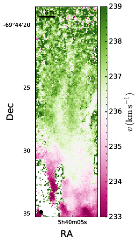
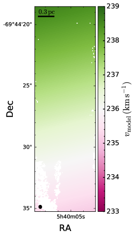
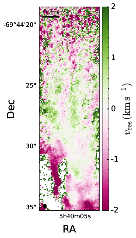
Figure 5: The left panel shows the ¹³CO moment-1 (intensity-weighted velocity) map of the analysis region. The velocity map shows a large-scale gradient from top to bottom that we subtract by modeling it with a gradient as shown in the middle panel. The right panel shows the residual velocities after the large-scale gradient subtraction, which represent random, turbulent motions within the gas. We use the residual velocities together with the second moment map to find the overall 1D velocity dispersion in the gas, $\sigma_{\rm{v,1D}}$.

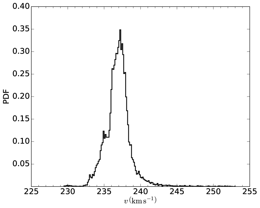
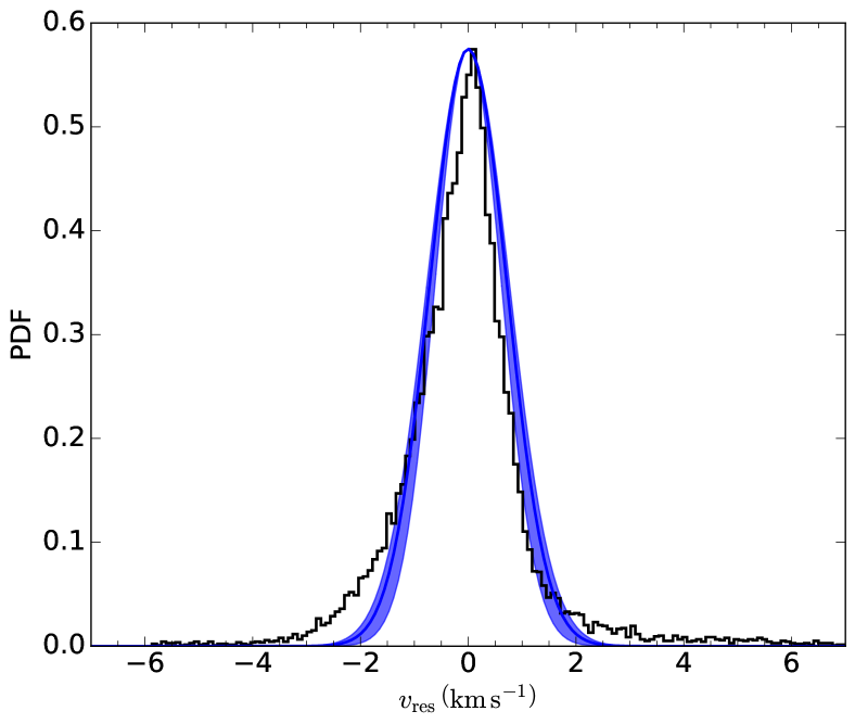
Figure 6: PDFs of the velocity before (left) and after (right) gradient subtraction. The PDF of the residuals post gradient subtraction is largely Gaussian. The blue-shaded curve denotes the $1\sigma$ range of the best-fit Gaussian in solid blue. The width of the best-fit Gaussian (denoted by $\sigma_{\mathrm{v,1D,res}}$) together with the second moment velocity dispersion (denoted by $\sigma_{\rm{v,1D,2m}}$) is used to determine the overall 1D velocity dispersion in the gas, $\sigma_{\mathrm{v,1D}}$ (see Table 1). We find $\sigma_{\mathrm{v,1D,res}}=(0.72\pm 0.05)\,\mathrm{km\,s^{-1}}$, and $\sigma_{\rm{v,1D}}=(0.94\pm 0.09)\,\rm{km\,s^{-1}}$.

3.1.4 Conversion from 2D to 3D density dispersion

To estimate the 3D density dispersion ($\sigma_{\rho/\rho_{0}}$) from the 2D column density dispersion ($\sigma_{N/N_{0}}$), we first measure the 2D column density power spectrum $P_{\mathrm{2D}}(k)$ of the quantity $N/N_{0}-1$, where $k=|\mathbf{k}|$ is the isotropic wavenumber. We use this to reconstruct the 3D density power spectrum $P_{\mathrm{3D}}(k)$ of the variable $\rho/\rho_{0}-1$, as $P_{\mathrm{3D}}(k)=2kP_{\mathrm{2D}}(k)$, assuming isotropy of the cloud (Brunt et al., 2010a, b; Kainulainen et al., 2014). The variance of a mean-zero field is proportional to the integral of the power spectrum over all $k$ (Arfken et al., 2013; Beattie & Federrath, 2020). This implies that the 2D column density dispersion, $\sigma_{N/N_{0}}$ and 3D density dispersion, $\sigma_{\rho/\rho_{0}}$ are equal to $\left[\int P_{\mathrm{2D}}(k)dk\right]^{1/2}$ and $\left[\int P_{\mathrm{3D}}(k)dk\right]^{1/2}$, respectively. If we define $\mathcal{R}=P_{\mathrm{2D}}(k)/P_{\mathrm{3D}}(k)$, $\sigma_{\rho/\rho_{0}}$ can be obtained from the relation

$$\sigma_{\rho/\rho_{0}}=\frac{\sigma_{N/N_{0}}}{\mathcal{\sqrt{R}}}\,.$$ (9)

Thus, $\mathcal{R}$ represents the degree of anisotropy at the scale at which we measure $b$. Brunt et al. (2010a) showed that equation 9 holds to within 10 per cent for isotropic, periodic fields, and is less accurate for non-periodic fields. We thus mimic a periodic dataset (Ossenkopf et al., 2008) by placing three mirrored copies of the column density map around itself in a periodic configuration. In the case of non-isotropic, periodic clouds, (for example, in the presence of anisotropic turbulence driving – Hansen et al. 2011, or strong mean magnetic fields – Beattie & Federrath 2020), the maximum uncertainty in the 2D-to-3D reconstruction for these cases is less than 40 per cent (Federrath et al., 2016, section 3.1.2), which is mostly noticed at lower turbulent Mach numbers than that we find below in Section 3.2. We use this upper limit as a systematic uncertainty in the 2D-to-3D reconstruction step in our analysis. Following this approach, we obtain a value of $\sqrt{\mathcal{R}}=0.20\pm 0.04$ and $0.15\pm 0.03$, thus $\sigma_{\rho/\rho_{0}}=2.97^{+1.50}_{-0.71}$ and $3.40^{+0.92}_{-0.63}$ from equation 9, for the LTE and the NLTE analyses, respectively. The first panels in each row of Figure 4 show the PDF of $\sigma_{\rho/\rho_{0}}$ over all the bootstrapping realisations for the two cases, with the dashed lines depicting the $16^{\rm{th}}$, $50^{\rm{th}}$, and $84^{\rm{th}}$ percentiles, respectively. We see that the NLTE analysis gives a slightly higher 3D density dispersion than the LTE analysis, but it is consistent within the errorbars.

3.2 Turbulent Mach number

The turbulent Mach number, $\mathcal{M}$, is defined as the ratio of the turbulent velocity dispersion in 3D, $\sigma_{\rm{v,3D}}$, to the sound speed, $c_{\rm{s}}$. The intensity-weighted velocity (moment 1) map ($v$) of ¹³CO of the analysis region reveals the presence of a systematic large-scale gradient in the gas, as we show in the left panel of Figure 5. To retrieve the turbulent motions within the gas, we fit a linear model ($v_{\rm{model}}$) to account for this large-scale systematic gradient and subtract it from the moment 1 map; the model is plotted in the middle panel of Figure 5. We then use the resulting residual map ($v_{\rm{res}}$), as shown in the right panel of Figure 5, to obtain the 1D velocity dispersion ($\sigma_{\rm{v,1D,res}}$) by modeling the PDF of the residual velocities as a Gaussian. Figure 6 shows the velocity PDFs before and after the subtraction of the large-scale gradient. Fitting the latter PDF with a Gaussian and using the resulting width as an estimate of $\sigma_{\rm{v,1D,res}}$, we obtain $\sigma_{\rm{v,1D,res}}=(0.72\pm 0.05)\,\rm{km\,s^{-1}}$. This technique has been used in several works (e.g., Federrath et al. 2016; Chen et al. 2018; Sharda et al. 2018; Sharda et al. 2019a, M21), and has been shown to be robust for deriving $\sigma_{\rm{v,1D,res}}$ provided the region is resolved with $\gtrsim 30$ resolution elements (Sharda et al., 2018).

However, there is no guarantee that residuals obtained from only removing the large-scale gradient represent the true random, turbulent motions within the cloud, since small-scale systematic motions or higher order moments can still persist and contribute to $\sigma_{\rm{v,1D,res}}$. In fact, we can see from the first and third panels of Figure 5 that gradient subtraction has a limited effect on the southern part of the analysis region, which is also reflected in the negative velocity tail in the PDF of $v_{\rm{res}}$ in the right panel of Figure 6. Recent work from Stewart & Federrath (2021) finds that the above approach likely underestimates the true velocity dispersion, and a combination of $\sigma_{\rm{v,1D,res}}$ and the second moment (intensity-weighted velocity dispersion around the mean) gives a better estimate of the true velocity dispersion. So, we define the overall 1D velocity dispersion as $\sigma_{\rm{v,1D}}=\sqrt{(\sigma_{\rm{v,1D,res}})^{2}+(\sigma_{\rm{v,1D,2m}})^{2}}$, where $\sigma_{\rm{v,1D,2m}}\approx 0.6\,\rm{km\,s^{-1}}$ is the velocity dispersion from the mean of the second moment of ¹³CO (F19). Thus, we obtain $\sigma_{\rm{v,1D}}=(0.94\pm 0.09)\,\rm{km\,s^{-1}}$. We then scale $\sigma_{\rm{v,1D}}$ by a factor $\sqrt{3}$ (assuming isotropic velocity fluctuations) to obtain the 3D velocity dispersion, $\sigma_{\rm{v,3D}}$. Using a combination of the gradient-subtracted first moment velocities and the second moment velocities to obtain the velocity dispersion rather than deriving it from the line shape in each pixel enables us to avoid the various biases that are introduced in line profiles; for example, flattened line centers due to opacity, overestimation of the turbulent Mach number due to opacity broadening, loss of line wings due to noise, or missing emission from low-density material due to excitation effects – Correia et al. 2014; Hacar et al. 2016; Yuan et al. 2020.

For the LTE case, the turbulent Mach number corresponding to $T_{\rm{g}}=(40\pm 10)\,\rm{K}$ is $\mathcal{M}=4.74^{+0.74}_{-0.54}$. For the NLTE case, we find $\mathcal{M}=3.92^{+0.35}_{-0.29}$ based on the best-fit $T_{\rm{g}}=(58\pm 8)\,\rm{K}$. The turbulent Mach numbers we obtain are indicative of supersonic turbulence in the region and closely follow the $\mathcal{M}-\theta$ relation from Hopkins (2013, figure 3). The middle panel in each row of Figure 4 depicts the distribution of $\mathcal{M}$ for the two cases based on 10,000 bootstrapping realisations; the dashed lines denote the quantiles for the $16^{\rm{th}}$, $50^{\rm{th}}$, and $84^{\rm{th}}$ percentiles, respectively.

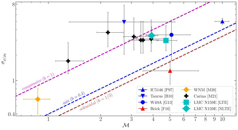
Figure 7: Plot summarizing currently available measurements of the mode of turbulence from observations, denoted by the ratio of the 3D density dispersion ($\sigma_{\rho/\rho_{0}}$) to the turbulent Mach number ($\mathcal{M}$). The three dashed lines mark the theoretical limits within which turbulence can be driven through solenoidal or compressive modes, or a mixture of the two (Federrath et al., 2008, 2010). The data is taken from various sources – IC5146 (Padoan et al., 1997a), Taurus (Brunt 2010, with revised estimates of the turbulent Mach number from Kainulainen & Tan 2013, and magnetic field estimate from Federrath et al. 2016), W49A (Ginsburg et al., 2013), CMZ cloud Brick (Federrath et al., 2016), Warm Neutral Medium (WNM, Marchal & Miville-Deschênes, 2021), and 6 pillar-like regions in the Carina Nebula (M21). Errors are shown where available. Note that only Taurus and Brick have magnetic field estimates available for them, so for these clouds the $x$-axis should be read as $\mathcal{M}(1+1/\beta)^{-1/2}$, where $\beta$ is the turbulent plasma beta that accounts for the effects of magnetic fields in deriving the mode of turbulence (Molina et al., 2012). The cyan markers denote the measurements for the LMC star-forming region N159E we study in this work using the LTE and the NLTE approaches; it is the only extragalactic region where the driving mode of turbulence has been measured.

4 Results

Thanks to the exquisite resolution provided by ALMA, we can now derive the first extragalactic measurement of the driving mode of turbulence in a star-forming region. For simplicity, we collect all the different parameters we derive in Table 1. Using the measured values of the width of gas volume density PDF, $\sigma_{\rho/\rho_{0}}$, and turbulent Mach number, $\mathcal{M}$, we can now estimate the driving mode parameter $b=0.62^{+0.34}_{-0.17}$ and $0.87^{+0.25}_{-0.17}$ for the LTE and the NLTE analyses, respectively. The right panels of the two rows in Figure 4 plots the distributions of $b$ resulting from the 10,000 bootstrapping realisations. These values of $b$ indicate the presence of primarily compressive (or, solenoidal-free) turbulence in the region. We also find that the more accurate NLTE analysis gives a higher $b$ as compared to the LTE analysis. Our findings (from the NLTE analysis) exclude a natural mix of modes and fully solenoidal driving at a $>6\sigma$ and $>7\sigma$ level, respectively.

It is worth noting that the distribution of $b$ in Figure 4 has a tail extending to $b>1$, which might seem in contradiction with theoretical expectations. While a part of the presence of this tail is simply due to observational and modeling uncertainties on various parameters, it could also be due to physical reasons. For example, it is possible that $b>1$ if a physical process other than turbulence (such as gravity) has substantial contributions to density fluctuations (and hence the density dispersion). It is also possible that the derived turbulent Mach number includes contributions from non-turbulent sources, such as gravitational collapse motions. M21 find that all of the pillars in the Carina Nebula where they derive $b>1$ have virial parameters < 1, suggesting that gravity plays a significant role in the density and velocity structure of gas in such pillars. On the other hand, Federrath et al. (2016) find $b<1/3$ for the Central Molecular Zone (CMZ) cloud Brick (also known as G0.253+0.016) due to strong shearing motions. Given the presence of dense cores like MMS-1 and MMS-2 in the analysis region, it is not surprising that the expected distribution of $b$ extends beyond unity. However, like our results, the uncertainties on the measurements of Federrath et al. (2016) and M21 are consistent with $1/3\leq b\leq 1$.

It is helpful to place our results in the context of the literature. Figure 7 shows a compilation of observations where the driving mode of turbulence has been measured in the Galaxy. The data are limited and heterogeneous because different studies use different gas density tracers. Most clouds (except for Taurus and Brick) lack an estimate of the magnetic field strength, thus we assume $\beta\to\infty$ for them. For Taurus, we use the magnetic field estimate from Federrath et al. (2016) that is based on earlier results from Heyer & Brunt (2012). We see two distinct classes of star-forming regions from Figure 7 – one where the turbulence is highly compressive in nature (like the spiral arm molecular cloud Taurus and the star-forming pillars in the Carina Nebula), and another where it is largely non-compressive (like the CMZ cloud Brick). Our NLTE measurements for N159E (the only extragalactic region on this plot) fall in the former category.

5 Caveats

The use of CO isotopologues to derive gas density PDFs typically introduces three major sources of uncertainty due to uncertain abundances, excitation temperatures, and fraction of CO-dark molecular gas. To test the impacts of abundance variations, we increase $X[\rm{H_{2}}/^{12}\mathrm{CO}]$ by a factor of 2 (e.g., Bolatto et al., 2013), finding that it slightly decreases $\sigma_{\rho/\rho_{0}}$ without significantly changing the turbulence driving parameter $b$. Similarly, if we increase $X[^{12}\mathrm{CO}/^{13}\mathrm{CO}]$ to 70 (typical of molecular clouds in the Galaxy – Johansson et al., 1994; Wilson & Rood, 1994; Yan et al., 2019), $\sigma_{\rho/\rho_{0}}$ decreases by at most 17 per cent, which is within the error bars. The reason our results are insensitive to variations in CO abundances is because we use a combination of optically-thick and optically-thin tracers in our analysis (see equation 5). Additionally, the NLTE analysis ensures that we self-consistently calculate the optical depth of the CO isotopologues, thus ensuring that the radiative transfer effects do not bias the resulting density dispersion (Burkhart et al., 2013). While we have to assume $T_{\rm{g}}=T_{\rm{ex}}$ in LTE, the NLTE modeling gives a self-consistent excitation temperature, thus suppressing the uncertainties in $T_{\rm{ex}}$. We cannot constrain the amount of CO-dark molecular gas (e.g., Glover & Clark, 2012), which can be quite high in low-metallicity regions like the LMC and the Small Magellanic Cloud (SMC; e.g., Roman-Duval et al., 2014; Jameson et al., 2018; Chevance et al., 2020; Tokuda et al., 2021). Nonetheless, given the detection of C¹⁸O in N159E, we do not expect to significantly underestimate high-density molecular gas within the region of interest. Thus, we find that the NLTE analysis mitigates some of the major caveats around assuming LTE. However, the LVG approximation used by the NLTE analysis can be problematic at very high CO column densities (Asensio Ramos & Elitzur, 2018). This is because it only returns the integrated brightness temperatures for each line by assuming a top-hat line profile, thus ignoring the wings in the velocity-resolved line profiles we observe in the data. It also assumes a constant optical depth and escape probability for a given line at all frequencies. Future modeling of molecular gas tracers should therefore aim at providing velocity-resolved line profiles that are now measurable by ALMA.

There are also some caveats in extracting gas column density and constructing density PDFs using CO isotopologues. For example, the dynamic range of a density PDF constructed using CO isotopologues is quite narrow as compared to that probed by dust (e.g., Schneider et al., 2013, 2015b). However, dust observations are typically at lower resolution than CO, and cannot be used to trace the gas kinematics (e.g., Goodman et al., 2009) or distinguish different clouds along the line of sight (e.g., Schneider et al., 2016). It has also been shown that density PDFs constructed using interferometric observations can create a spurious low-density tail due to the direct current (DC) offset inherent to interferometry, and as a result can produce a PDF that is wider than the true PDF (Ossenkopf-Okada et al., 2016). Thus, it is quite possible that ALMA’s interferometric data leads to an overestimation of $b$. We have also ignored the effects of magnetic fields throughout this analysis. If significant, magnetic fields would lead to an increase in $b$, thereby favouring a more compressive turbulent driving (Padoan & Nordlund, 2011; Federrath & Klessen, 2012; Molina et al., 2012). For example, if we follow Crutcher (2012) to get a rough estimate of the magnetic field strength based on the mean column density in the region, we find a field strength $\sim 100\,\rm{\mu G}$. This field strength corresponds to turbulent plasma $\beta\sim 3.5$ for the mean density corresponding to the NLTE case, thus giving $b\sim 0.98$. Since magnetic fields and possible overestimation of $\sigma_{\rho/\rho_{0}}$ due to interferometric effects alter $b$ in opposite directions, we speculate that their effects on the driving mode roughly balance out. However, it is difficult to predict the exact changes in $b$ without an accurate estimate of the magnetic field strength. Future observations (for example, using Faraday rotation measure – Gaensler et al. 2005; Mao et al. 2012; Livingston et al. 2021) will provide critical constraints on the magnetic field strength in resolved regions within the Magellanic Clouds.

6 Possible drivers of compressive turbulence in N159E

If the density structure and the dynamics we see in N159E is highly influenced by gravitational collapse motions, then we naturally expect a large fraction of compressive modes to be introduced, which may explain the high value of $b$ (Jaupart & Chabrier, 2020; Khullar et al., 2021). Several studies have shown how supersonic turbulence can compress the gas on local scales leading to the creation of cores (such as MMS-1 and MMS-2 in N159E) and filaments, while stabilizing the cloud against gravity on larger scales (e.g., Ossenkopf & Mac Low, 2002; Schneider et al., 2011; Federrath & Klessen, 2012; Robertson & Goldreich, 2018; Beattie et al., 2020; Imara et al., 2021). To verify whether this is indeed the case, we require observations of molecular gas tracers for higher densities (e.g., HCN or HCO⁺) at similar resolution and sensitivity as the CO observations we use in this study. This is because such tracers can potentially reveal the power-law tail in the density PDF due to self-gravitating structures, such as the MMS-1 and MMS-2 cores.

Another plausible candidate for compressive driving is the compression caused by the H $I$1.2ex  flow that is proposed to have led to the creation of the massive molecular filaments observed by ALMA ( F19, figure 8), a view supported by magnetohydrodynamical simulations (Inoue & Inutsuka, 2012; Inoue & Fukui, 2013). This flow is proposed to have originated due to tidal interactions between the LMC and SMC (Bekki & Chiba, 2007; Fukui et al., 2017) $0.2\,\rm{Gyr}$ ago (Fujimoto & Noguchi, 1990). However, the limited resolution of currently available H $I$1.2ex  data (Kim et al., 2003) makes it challenging to study the correlation between the molecular gas structure observed by ALMA and the larger-scale H $I$1.2ex  gas structure (e.g., Fukui et al., 2009). Note that N159E is only one part of the GMC N159. The western end of N159 (denoted by N159W in the literature – Heikkila et al. 1998) shows similar molecular gas morphology, protostellar activity, and star formation activity (Tokuda et al., 2019). These similarities hint at a common origin of the kinematics and dynamics in both N159E and N159W, providing support for the large-scale H $I$1.2ex  flow scenario (F19). Even if N159W also exhibits largely compressive turbulence, it is difficult to establish whether the H $I$1.2ex  flow that originated $0.2\,\rm{Gyr}$ ago is the cause, given the instantaneous nature of the mode of turbulence that we can measure from observations. High-resolution H $I$1.2ex  observations from the H $I$1.2ex  component of the upcoming Galactic ASKAP survey (GASKAP-H $I$1.2ex  – Dickey et al. 2013; Pingel et al. 2021) and eventual SKA observations (Koribalski et al., 2020) will prove instrumental in pinpointing the driver of compressive turbulence in N159E.

As we noted in Section 1, protostellar outflows can also drive and inject turbulence in star-forming regions. Simulations find that protostellar outflows drive primarily solenoidal motions, at least in the shearing layers between outflow and ambient gas (Offner & Arce, 2014; Offner & Chaban, 2017), while the bow shock of an outflow is more compressive (e.g., Guicking et al., 2010). However, the protostellar outflows observed in N159E are only $\sim 0.1\,\rm{pc}$ in size (F19), so we do not expect them to drive turbulence in our analysis region, which is $10\times$ bigger (see Figure 1). Thus, we can exclude them as a source of the compressive driving of turbulence in this region.

Lastly, it is worth emphasizing that turbulence driving in other parts of N159E not covered in this work may not be compressive, or may not share the same physical origin for compressive driving as the analysis region. For example, it is likely that the CO pillars surrounding the Papillon YSO (magenta box in Figure 1) also exhibit compressive turbulence driving, but due to photoionization feedback from the YSOs, similar to the CO pillars in the Carina nebula in the Milky Way (M21).

7 Conclusions

In this work, we utilize high-resolution (sub-pc) ALMA ¹²CO ($J$ = 2–1), ¹³CO ($J$ = 2–1), and C¹⁸O ($J$ = 2–1) observations of the star-forming region N159E (the Papillon Nebula) in the LMC to provide the first extragalactic measurement of turbulence driving at pc scales. The turbulence driving mode is characterized by the parameter $b$ – the ratio of the normalized gas density dispersion ($\sigma_{\rho/\rho_{0}}$) to the turbulent Mach number ($\mathcal{M}$). Values of $b\approx 1/3$ represent a highly solenoidal driving, $b\approx 1$ represents highly compressive driving, and a natural mixture of the two is given by $b\approx 0.4$ (Federrath et al., 2008, 2010).

We use an NLTE analysis of the CO isotopologues using the radiative transfer code DESPOTIC (Krumholz, 2014) to construct the gas column density PDF for the analysis region we show in Figure 1, which consists of filamentary molecular clouds with dense cores driving protostellar outflows. We then fit the PDF with the Hopkins (2013) density PDF model to get the 2D column density dispersion, which we then convert to get the 3D density dispersion using the Brunt et al. (2010a) method. We obtain $\sigma_{\rho/\rho_{0}}=3.4^{+0.92}_{-0.63}$. We use a combination of the gradient-subtracted first moment map and the mean of the second moment map to get the gas velocity dispersion, which gives $\mathcal{M}=3.9^{+0.35}_{-0.29}$. Thus, the driving mode of turbulence we obtain is $b=0.87^{+0.25}_{-0.17}$, indicating that the turbulence being driven in this region is highly compressive. We suspect that the compressive turbulence could be driven by gravo-turbulent fragmentation of the dense gas, or by the H $I$1.2ex  flow that is proposed to have led to the creation of GMC N159. This analysis is easily reproducible and can be applied to measure $b$ in resolved star-forming regions both in the local and the high-redshift Universe.

Data Availability Statement

No new data were generated for this work. The ALMA data we use in this work is publicly available here.

Appendix A Mocz and Burkhart (2019) non-lognormal density model

A.1 Model description

Mocz & Burkhart (2019) model the volume-weighted density PDF of hydrodynamical density fluctuations using a Markovian framework. They construct a Langevin model

$$s(t+dt) =s(t)+A(s)\operatorname{d}\!{t}+\mathcal{N}(0,1)\sqrt{D(s)\operatorname{d}\!{t}},$$ (10)

$$A(s) =-\frac{s-s_{0}}{\tau_{A}}\left[1+H(s-s_{0})\frac{3f}{2}\right],$$ (11)

$$D(s) =\frac{2\sigma_{s}^{2}}{\tau_{0}},$$ (12)

where $A(s)$ is the deterministic, or advective term in the model, $D(s)$ is the stochastic, or diffusive term in the model and $\mathcal{N}(0,1)$ is a standard normal distribution. The stochastic term, $D(s)$, contains the turbulent fluctuations $\sigma_{s}^{2}$, which have dynamical time-scale $\tau_{0}=\ell_{\rm 0}/(c_{s}\operatorname{\mathcal{M}})$, where $\ell_{\rm 0}$ is the turbulent driving scale. The deterministic term, $A(s)$, encodes how logarithmic density fluctuates about the mean dynamically on timescales $\tau_{A}=\tau_{A,0}/[1+H(s-s_{0,V})\frac{3f}{2}]$, where $H(s-s_{0})$ is the Heaviside function. This encodes how high-density structures, such as the density contrast caused by a shock, live on shorter times scales than the rest of the density fluctuations in the fluid (Robertson & Goldreich, 2018). For $s>s_{0}$ the timescale is reduced by $\tau_{A}=3f/2$, and hence $f$ becomes the fitting parameter for how much shorter the dynamical timescales are for the over-dense regions. The PDF of Mocz & Burkhart (2019)’s Langevin model defines a steady-state solution to the Fokker-Planck equation (Kadanoff, 2000), which has a solution of the form,

$$p_{\rm MB}(s) \propto\exp\left\{-\frac{(s-s_{0})^{2}[1+f(s-s_{0})H(s-s_{0})]}{2\sigma_{s}^{2}(\tau_{A}/\tau_{0})}\right\}.$$ (13)

The asymmetric dynamical timescale of the low- and high-density objects in the cloud encodes a non-Gaussian 3^rd moment (skewness) into the PDF through the $\mathcal{O}([s-s_{0}]^{3})$ term in the exponential.

A.2 Fitting and Results

We fit equation 13 using the same bootstrapping method we used to fit the Hopkins (2013) PDF model in Section 3.1.3. Each fit in the bootstrapped sample preserves probability, $\int\operatorname{d}\!{\eta}\,p_{\rm MB}(\eta)=1$, $\int\operatorname{d}\!{\eta}\,e^{\eta}p_{\rm MB}(\eta)=N_{0}$. Our fit results, $\sigma_{N/N_{0}}=0.56\pm 0.37$ and $f=3.15\pm 0.42$, are consistent within $1\sigma$ variations to the results quoted in Table 1, and hence our measurements of the density dispersion are robust to different non-lognormal density PDF models.

References

- Abe et al. (2021) Abe D., Inoue T., Inutsuka S.-i., Matsumoto T., 2021, ApJ, 916, 83
- Arfken et al. (2013) Arfken G. B., Weber H. J., Harris F. E., 2013, in Arfken G. B., Weber H. J., Harris F. E., eds, , Mathematical Methods for Physicists (Seventh Edition), seventh edition edn, Academic Press, Boston, pp 935 – 962
- Asensio Ramos & Elitzur (2018) Asensio Ramos A., Elitzur M., 2018, A&A, 616, A131
- Astropy Collaboration et al. (2013) Astropy Collaboration et al., 2013, A&A, 558, A33
- Astropy Collaboration et al. (2018) Astropy Collaboration et al., 2018, AJ, 156, 123
- Beattie & Federrath (2020) Beattie J. R., Federrath C., 2020, MNRAS, 492, 668
- Beattie et al. (2020) Beattie J. R., Federrath C., Seta A., 2020, MNRAS, 498, 1593
- Beattie et al. (2021a) Beattie J. R., Mocz P., Federrath C., Klessen R. S., 2021a, arXiv e-prints, p. arXiv:2109.10470
- Beattie et al. (2021b) Beattie J. R., Mocz P., Federrath C., Klessen R. S., 2021b, MNRAS, 504, 4354
- Bekki & Chiba (2007) Bekki K., Chiba M., 2007, Publ. Astron. Soc. Australia, 24, 21
- Bolatto et al. (2013) Bolatto A. D., Wolfire M., Leroy A. K., 2013, ARA&A, 51, 207
- Brunt (2010) Brunt C. M., 2010, A&A, 513, A67
- Brunt et al. (2010a) Brunt C. M., Federrath C., Price D. J., 2010a, MNRAS, 403, 1507
- Brunt et al. (2010b) Brunt C. M., Federrath C., Price D. J., 2010b, MNRAS, 405, L56
- Burkhart (2018) Burkhart B., 2018, ApJ, 863, 118
- Burkhart & Lazarian (2012) Burkhart B., Lazarian A., 2012, ApJ, 755, L19
- Burkhart & Mocz (2019) Burkhart B., Mocz P., 2019, ApJ, 879, 129
- Burkhart et al. (2009) Burkhart B., Falceta-Gonçalves D., Kowal G., Lazarian A., 2009, ApJ, 693, 250
- Burkhart et al. (2013) Burkhart B., Ossenkopf V., Lazarian A., Stutzki J., 2013, ApJ, 771, 122
- Burkhart et al. (2015) Burkhart B., Collins D. C., Lazarian A., 2015, ApJ, 808, 48
- Burkhart et al. (2017) Burkhart B., Stalpes K., Collins D. C., 2017, ApJ, 834, L1
- Burkhart et al. (2020) Burkhart B., et al., 2020, ApJ, 905, 14
- Chen et al. (2010) Chen C. H. R., et al., 2010, ApJ, 721, 1206
- Chen et al. (2018) Chen H. H.-H., Burkhart B., Goodman A., Collins D. C., 2018, ApJ, 859, 162
- Chevance et al. (2020) Chevance M., et al., 2020, MNRAS, 494, 5279
- Choi et al. (1993) Choi M., Evans Neal J. I., Jaffe D. T., 1993, ApJ, 417, 624
- Collins et al. (2012) Collins D. C., Kritsuk A. G., Padoan P., Li H., Xu H., Ustyugov S. D., Norman M. L., 2012, ApJ, 750, 13
- Correia et al. (2014) Correia C., Burkhart B., Lazarian A., Ossenkopf V., Stutzki J., Kainulainen J., Kowal G., de Medeiros J. R., 2014, ApJ, 785, L1
- Crutcher (2012) Crutcher R. M., 2012, ARA&A, 50, 29
- Dickey et al. (2013) Dickey J. M., et al., 2013, Publ. Astron. Soc. Australia, 30, e003
- Federrath (2016) Federrath C., 2016, MNRAS, 457, 375
- Federrath & Banerjee (2015) Federrath C., Banerjee S., 2015, MNRAS, 448, 3297
- Federrath & Klessen (2012) Federrath C., Klessen R. S., 2012, ApJ, 761, 156
- Federrath & Klessen (2013) Federrath C., Klessen R. S., 2013, ApJ, 763, 51
- Federrath et al. (2008) Federrath C., Klessen R. S., Schmidt W., 2008, ApJ, 688, L79
- Federrath et al. (2010) Federrath C., Roman-Duval J., Klessen R. S., Schmidt W., Mac Low M. M., 2010, A&A, 512, A81
- Federrath et al. (2011) Federrath C., Chabrier G., Schober J., Banerjee R., Klessen R. S., Schleicher D. R. G., 2011, Phys. Rev. Lett., 107, 114504
- Federrath et al. (2016) Federrath C., et al., 2016, ApJ, 832, 143
- Federrath et al. (2017) Federrath C., et al., 2017, in Crocker R. M., Longmore S. N., Bicknell G. V., eds, Vol. 322, The Multi-Messenger Astrophysics of the Galactic Centre. pp 123–128 (arXiv:1609.08726), doi:10.1017/S1743921316012357
- Federrath et al. (2021) Federrath C., Klessen R. S., Iapichino L., Beattie J. R., 2021, Nature Astronomy, 5, 365
- Finn et al. (2021) Finn M. K., et al., 2021, ApJ, 917, 106
- Fischera (2014) Fischera J., 2014, A&A, 565, A24
- Fujimoto & Noguchi (1990) Fujimoto M., Noguchi M., 1990, PASJ, 42, 505
- Fukui et al. (2008) Fukui Y., et al., 2008, ApJS, 178, 56
- Fukui et al. (2009) Fukui Y., et al., 2009, ApJ, 705, 144
- Fukui et al. (2015) Fukui Y., et al., 2015, ApJ, 807, L4
- Fukui et al. (2017) Fukui Y., Tsuge K., Sano H., Bekki K., Yozin C., Tachihara K., Inoue T., 2017, PASJ, 69, L5
- Fukui et al. (2019) Fukui Y., et al., 2019, ApJ, 886, 14 (F19)
- Fukui et al. (2021) Fukui Y., Habe A., Inoue T., Enokiya R., Tachihara K., 2021, PASJ, 73, S1
- Gaensler et al. (2005) Gaensler B. M., Haverkorn M., Staveley-Smith L., Dickey J. M., McClure-Griffiths N. M., Dickel J. R., Wolleben M., 2005, Science, 307, 1610
- Galametz et al. (2020) Galametz M., et al., 2020, A&A, 643, A63
- Gatley et al. (1981) Gatley I., Becklin E. E., Hyland A. R., Jones T. J., 1981, MNRAS, 197, 17
- Ginsburg et al. (2013) Ginsburg A., Federrath C., Darling J., 2013, ApJ, 779, 50
- Girichidis et al. (2014) Girichidis P., Konstandin L., Whitworth A. P., Klessen R. S., 2014, ApJ, 781, 91
- Girichidis et al. (2020) Girichidis P., et al., 2020, Space Sci. Rev., 216, 68
- Glover & Clark (2012) Glover S. C. O., Clark P. C., 2012, MNRAS, 426, 377
- Goldsmith & Langer (1999) Goldsmith P. F., Langer W. D., 1999, ApJ, 517, 209
- Goodman et al. (2009) Goodman A. A., Pineda J. E., Schnee S. L., 2009, ApJ, 692, 91
- Guicking et al. (2010) Guicking L., Glassmeier K.-H., Auster H.-U., Delva M., Motschmann U., Narita Y., Zhang T. L., 2010, Annales Geophysicae, 28, 951
- Hacar et al. (2016) Hacar A., Alves J., Burkert A., Goldsmith P., 2016, A&A, 591, A104
- Hansen et al. (2011) Hansen C. E., McKee C. F., Klein R. I., 2011, ApJ, 738, 88
- Hansen et al. (2012) Hansen C. E., Klein R. I., McKee C. F., Fisher R. T., 2012, ApJ, 747, 22
- Harris et al. (2020) Harris C. R., et al., 2020, Nature, 585, 357
- Heikkila et al. (1998) Heikkila A., Johansson L. E. B., Olofsson H., 1998, A&A, 332, 493
- Heydari-Malayeri et al. (1999) Heydari-Malayeri M., Rosa M. R., Charmandaris V., Deharveng L., Zinnecker H., 1999, A&A, 352, 665
- Heyer & Brunt (2012) Heyer M. H., Brunt C. M., 2012, MNRAS, 420, 1562
- Hopkins (2013) Hopkins P. F., 2013, MNRAS, 430, 1880
- Hughes et al. (1998) Hughes J. P., Hayashi I., Koyama K., 1998, ApJ, 505, 732
- Hughes et al. (2010) Hughes A., et al., 2010, MNRAS, 406, 2065
- Hunter (2007) Hunter J. D., 2007, Computing in Science & Engineering, 9, 90
- Imara et al. (2021) Imara N., Forbes J. C., Weaver J. C., 2021, ApJ, 918, L3
- Immer et al. (2016) Immer K., Kauffmann J., Pillai T., Ginsburg A., Menten K. M., 2016, A&A, 595, A94
- Indebetouw et al. (2004) Indebetouw R., Johnson K. E., Conti P., 2004, AJ, 128, 2206
- Indebetouw et al. (2013) Indebetouw R., et al., 2013, ApJ, 774, 73
- Inoue & Fukui (2013) Inoue T., Fukui Y., 2013, ApJ, 774, L31
- Inoue & Inutsuka (2012) Inoue T., Inutsuka S.-i., 2012, ApJ, 759, 35
- Inoue et al. (2018) Inoue T., Hennebelle P., Fukui Y., Matsumoto T., Iwasaki K., Inutsuka S.-i., 2018, PASJ, 70, S53
- Jameson et al. (2018) Jameson K. E., et al., 2018, ApJ, 853, 111
- Jaupart & Chabrier (2020) Jaupart E., Chabrier G., 2020, ApJ, 903, L2
- Jin et al. (2017) Jin K., Salim D. M., Federrath C., Tasker E. J., Habe A., Kainulainen J. T., 2017, MNRAS, 469, 383
- Johansson et al. (1994) Johansson L. E. B., Olofsson H., Hjalmarson A., Gredel R., Black J. H., 1994, A&A, 291, 89
- Kadanoff (2000) Kadanoff L. P., 2000, Statistical Physics. Vol. 1, World Scientific, Singapore, doi:https://doi.org/10.1142/4016
- Kainulainen & Federrath (2017) Kainulainen J., Federrath C., 2017, A&A, 608, L3
- Kainulainen & Tan (2013) Kainulainen J., Tan J. C., 2013, A&A, 549, A53
- Kainulainen et al. (2013) Kainulainen J., Federrath C., Henning T., 2013, A&A, 553, L8
- Kainulainen et al. (2014) Kainulainen J., Federrath C., Henning T., 2014, Science, 344, 183
- Khullar et al. (2021) Khullar S., Federrath C., Krumholz M. R., Matzner C. D., 2021, MNRAS, 507, 4335
- Kim et al. (2003) Kim S., Staveley-Smith L., Dopita M. A., Sault R. J., Freeman K. C., Lee Y., Chu Y.-H., 2003, ApJS, 148, 473
- Konstandin et al. (2012) Konstandin L., Girichidis P., Federrath C., Klessen R. S., 2012, ApJ, 761, 149
- Konstandin et al. (2016) Konstandin L., Schmidt W., Girichidis P., Peters T., Shetty R., Klessen R. S., 2016, MNRAS, 460, 4483
- Koribalski et al. (2020) Koribalski B. S., et al., 2020, Ap&SS, 365, 118
- Körtgen (2020) Körtgen B., 2020, MNRAS, 497, 1263
- Körtgen et al. (2017) Körtgen B., Federrath C., Banerjee R., 2017, MNRAS, 472, 2496
- Körtgen et al. (2019) Körtgen B., Federrath C., Banerjee R., 2019, MNRAS, 482, 5233
- Kowal et al. (2007) Kowal G., Lazarian A., Beresnyak A., 2007, ApJ, 658, 423
- Kritsuk et al. (2011) Kritsuk A. G., Norman M. L., Wagner R., 2011, ApJ, 727, L20
- Krumholz (2014) Krumholz M. R., 2014, MNRAS, 437, 1662
- Krumholz & McKee (2005) Krumholz M. R., McKee C. F., 2005, ApJ, 630, 250
- Lim et al. (2020) Lim J., Cho J., Yoon H., 2020, ApJ, 893, 75
- Livingston et al. (2021) Livingston J. D., McClure-Griffiths N. M., Mao S. A., Ma Y. K., Gaensler B. M., Heald G., Seta A., 2021, MNRAS, submitted
- Mandal et al. (2020) Mandal A., Federrath C., Körtgen B., 2020, MNRAS, 493, 3098
- Mangum & Shirley (2015) Mangum J. G., Shirley Y. L., 2015, PASP, 127, 266
- Mao et al. (2012) Mao S. A., et al., 2012, ApJ, 759, 25
- Marchal & Miville-Deschênes (2021) Marchal A., Miville-Deschênes M.-A., 2021, ApJ, 908, 186
- Menon et al. (2020) Menon S. H., Federrath C., Kuiper R., 2020, MNRAS, 493, 4643
- Menon et al. (2021) Menon S. H., Federrath C., Klaassen P., Kuiper R., Reiter M., 2021, MNRAS, 500, 1721 (M21)
- Meynadier et al. (2004) Meynadier F., Heydari-Malayeri M., Deharveng L., Charmandaris V., Le Bertre T., Rosa M. R., Schaerer D., Zinnecker H., 2004, A&A, 422, 129
- Miesch & Toomre (2009) Miesch M. S., Toomre J., 2009, Annual Review of Fluid Mechanics, 41, 317
- Minamidani et al. (2008) Minamidani T., et al., 2008, ApJS, 175, 485
- Mizuno et al. (2010) Mizuno Y., et al., 2010, PASJ, 62, 51
- Mocz & Burkhart (2019) Mocz P., Burkhart B., 2019, ApJ, 884, L35
- Mohapatra & Sharma (2019) Mohapatra R., Sharma P., 2019, MNRAS, 484, 4881
- Mohapatra et al. (2020) Mohapatra R., Federrath C., Sharma P., 2020, MNRAS, 493, 5838
- Molina et al. (2012) Molina F. Z., Glover S. C. O., Federrath C., Klessen R. S., 2012, MNRAS, 423, 2680
- Nakajima et al. (2005) Nakajima Y., et al., 2005, AJ, 129, 776
- Nayak et al. (2018) Nayak O., Meixner M., Fukui Y., Tachihara K., Onishi T., Saigo K., Tokuda K., Harada R., 2018, ApJ, 854, 154
- Nolan et al. (2015) Nolan C. A., Federrath C., Sutherland R. S., 2015, MNRAS, 451, 1380
- Offner & Arce (2014) Offner S. S. R., Arce H. G., 2014, ApJ, 784, 61
- Offner & Chaban (2017) Offner S. S. R., Chaban J., 2017, ApJ, 847, 104
- Offner & Liu (2018) Offner S. S. R., Liu Y., 2018, Nature Astronomy, 2, 896
- Oliphant (2006) Oliphant T. E., 2006, A guide to NumPy. Vol. 1, Trelgol Publishing USA
- Orkisz et al. (2017) Orkisz J. H., et al., 2017, A&A, 599, A99
- Ossenkopf & Mac Low (2002) Ossenkopf V., Mac Low M. M., 2002, A&A, 390, 307
- Ossenkopf-Okada et al. (2016) Ossenkopf-Okada V., Csengeri T., Schneider N., Federrath C., Klessen R. S., 2016, A&A, 590, A104
- Ossenkopf et al. (2008) Ossenkopf V., Krips M., Stutzki J., 2008, A&A, 485, 917
- Padoan & Nordlund (2011) Padoan P., Nordlund Å., 2011, ApJ, 730, 40
- Padoan et al. (1997a) Padoan P., Nordlund A., Jones B. J. T., 1997a, MNRAS, 288, 145
- Padoan et al. (1997b) Padoan P., Jones B. J. T., Nordlund Å. P., 1997b, ApJ, 474, 730
- Pan & Padoan (2009) Pan L., Padoan P., 2009, ApJ, 692, 594
- Pan et al. (2016) Pan L., Padoan P., Haugbølle T., Nordlund Å., 2016, ApJ, 825, 30
- Passot & Vázquez-Semadeni (1998) Passot T., Vázquez-Semadeni E., 1998, Phys. Rev. E, 58, 4501
- Pietrzyński et al. (2019) Pietrzyński G., et al., 2019, Nature, 567, 200
- Pingel et al. (2021) Pingel N. M., Dempsey J., McClure-Griffiths N. M., et al., 2021, Publ. Astron. Soc. Australia, submitted
- Robertson & Goldreich (2018) Robertson B., Goldreich P., 2018, ApJ, 854, 88
- Roman-Duval et al. (2014) Roman-Duval J., et al., 2014, ApJ, 797, 86
- Rosen et al. (2020) Rosen A. L., Offner S. S. R., Sadavoy S. I., Bhandare A., Vázquez-Semadeni E., Ginsburg A., 2020, Space Sci. Rev., 216, 62
- Saigo et al. (2017) Saigo K., et al., 2017, ApJ, 835, 108
- Salim et al. (2015) Salim D. M., Federrath C., Kewley L. J., 2015, ApJ, 806, L36
- Scannapieco & Safarzadeh (2018) Scannapieco E., Safarzadeh M., 2018, ApJ, 865, L14
- Schenck et al. (2016) Schenck A., Park S., Post S., 2016, AJ, 151, 161
- Schneider et al. (2011) Schneider N., et al., 2011, A&A, 529, A1
- Schneider et al. (2013) Schneider N., et al., 2013, ApJ, 766, L17
- Schneider et al. (2015a) Schneider N., et al., 2015a, MNRAS, 453, L41
- Schneider et al. (2015b) Schneider N., et al., 2015b, A&A, 578, A29
- Schneider et al. (2016) Schneider N., et al., 2016, A&A, 587, A74
- Schöier et al. (2005) Schöier F. L., van der Tak F. F. S., van Dishoeck E. F., Black J. H., 2005, A&A, 432, 369
- Seale et al. (2009) Seale J. P., Looney L. W., Chu Y.-H., Gruendl R. A., Brandl B., Chen C. H. R., Brandner W., Blake G. A., 2009, ApJ, 699, 150
- Sharda et al. (2018) Sharda P., Federrath C., da Cunha E., Swinbank A. M., Dye S., 2018, MNRAS, 477, 4380
- Sharda et al. (2019a) Sharda P., et al., 2019a, MNRAS, 487, 4305
- Sharda et al. (2019b) Sharda P., Krumholz M. R., Federrath C., 2019b, MNRAS, 490, 513
- Sharda et al. (2020) Sharda P., Federrath C., Krumholz M. R., 2020, MNRAS, 497, 336
- Sharda et al. (2021) Sharda P., Federrath C., Krumholz M. R., Schleicher D. R. G., 2021, MNRAS, 503, 2014
- Sobolev (1960) Sobolev V. V., 1960, Moving envelopes of stars. Harvard University Press
- Squire & Hopkins (2017) Squire J., Hopkins P. F., 2017, MNRAS, 471, 3753
- Stewart & Federrath (2021) Stewart M., Federrath C., 2021, MNRAS, submitted
- Struck & Smith (1999) Struck C., Smith D. C., 1999, ApJ, 527, 673
- Tang et al. (2017) Tang X. D., et al., 2017, A&A, 600, A16
- Tang et al. (2021) Tang X. D., et al., 2021, arXiv e-prints, p. arXiv:2108.10519
- Testor et al. (2006) Testor G., Lemaire J. L., Field D., Diana S., 2006, A&A, 453, 517
- Testor et al. (2007) Testor G., Lemaire J. L., Kristensen L. E., Field D., Diana S., 2007, A&A, 469, 459
- Tokuda et al. (2019) Tokuda K., et al., 2019, ApJ, 886, 15
- Tokuda et al. (2021) Tokuda K., et al., 2021, arXiv e-prints, p. arXiv:2108.09018
- Virtanen et al. (2020) Virtanen P., et al., 2020, Nature Methods, 17, 261
- Wang et al. (2009) Wang M., Chin Y. N., Henkel C., Whiteoak J. B., Cunningham M., 2009, ApJ, 690, 580
- Wilson & Rood (1994) Wilson T. L., Rood R., 1994, ARA&A, 32, 191
- Yan et al. (2019) Yan Y. T., et al., 2019, ApJ, 877, 154
- Yuan et al. (2020) Yuan Y., Krumholz M. R., Burkhart B., 2020, MNRAS, 498, 2440
- Zhuravleva et al. (2014) Zhuravleva I., et al., 2014, Nature, 515, 85
- de Jong et al. (1975) de Jong T., Chu S., Dalgarno A., 1975, ApJ, 199, 69
- de Jong et al. (1980) de Jong T., Boland W., Dalgarno A., 1980, A&A, 91, 68
- van der Tak et al. (2007) van der Tak F. F. S., Black J. H., Schöier F. L., Jansen D. J., van Dishoeck E. F., 2007, A&A, 468, 627
- van der Tak et al. (2020) van der Tak F. F. S., Lique F., Faure A., Black J. H., van Dishoeck E. F., 2020, Atoms, 8, 15