Sensitive Samples Revisited: Detecting Neural
Network Attacks Using Constraint Solvers

Abstract

Neural Networks are used today in numerous security- and safety-relevant domains and are, as such, a popular target of attacks that subvert their classification capabilities, by manipulating the network parameters. Prior work has introduced sensitive samples—inputs highly sensitive to parameter changes—to detect such manipulations, and proposed a gradient ascent-based approach to compute them. In this paper we offer an alternative, using symbolic constraint solvers. We model the network and a formal specification of a sensitive sample in the language of the solver and ask for a solution. This approach supports a rich class of queries, corresponding, for instance, to the presence of certain types of attacks. Unlike earlier techniques, our approach does not depend on convex search domains, or on the suitability of a starting point for the search. We address the performance limitations of constraint solvers by partitioning the search space for the solver, and exploring the partitions according to a balanced schedule that still retains completeness of the search. We demonstrate the impact of the use of solvers in terms of functionality and search efficiency, using a case study for the detection of Trojan attacks on Neural Networks.

1 Introduction

Given recent advances in the field of Deep Learning, Neural Networks (DNN)—the preferred data structure for many learning tasks—are used today in numerous application areas, including security- and safety-relevant domains. Their use by unsuspecting end users increasingly makes them the target of attacks that manipulate (a small fraction of) the network parameters, attempting to override the decision-making functionality of the network, at least for some inputs. Examples include the hijacking of image recognition software for access control, and the misguidance of autonomous vehicles. Society has a vital interest in detecting these kind of attacks, in order to mitigate or prevent them.

Inspired by recent work by He et al. [8], we consider in this paper the “cloud scenario”: the defender is the designer of the network, with full access to all parameters and the training data. To facilitate wide-spread use, after training they deploy the network using some DNN inference cloud service, which can, however, ultimately not be trusted. They therefore wish to determine inputs, called sensitive samples [8], that are sensitive to parameter manipulations and thus able to distinguish the original, trusted network, $N$, from a manipulated one, $N^{\prime}$.

In the aforementioned recent work, a sensitive sample $X^{\ast}$ is defined as an input that maximizes the difference between $N$ and $N^{\prime}$, resulting in an optimization problem. Provided the sample space is convex, $X^{\ast}$ can be found using (projected) gradient ascent (PGA). PGA is an efficient technique, but it is also—from a user perspective—somewhat demanding: in addition to the convexity of the sample space, we must compute the differential of the objective function, as well as the projection into the sample space, both of which can be numerically hard problems.

The goal of this paper is to cast the task of finding sensitive samples as a Boolean satisfiability modulo real arithmetic problem, and use an SMT solver to crack it. Such solvers do not require convex search spaces, and they are black boxes: finding a solution for the specified satisfiability (“sat”) problem is left entirely to the solver.

The flexibility of SMT solving does not come for free. Our sat problem locks as follows: given the network $N$, find a sensitive sample $X_{s}$ such that for all networks $N^{\prime}$ s.t. $N^{\prime}\not=N$, we have $N(X_{s})\not=N^{\prime}(X_{s})$. This is in fact a sat problem in a quantified logic. We approximate it by restricting the domain of adversarial networks $N^{\prime}$ to come from some type of attack commonly applied to $N$, such as a Trojan attack [11]. We build a representative Trojan-attack model $N^{\prime}$ and obtain a sat problem over quantifier-free Boolean logic modulo real arithmetic. Input $X_{s}$ has qualities resembling a test case for detecting the attack: if positive, the attack is present; if negative, we cannot fully guarantee the integrity of the cloud model $N^{\prime}$.

The second challenge with using SMT solvers is that, given their symbolic nature, they cannot compete in efficiency with “concrete” evaluation-based solvers like PGA-based search engines. The bottleneck in the SMT solving process is the presence of ReLU (“rectified linear unit”; see Sec. A.1) activation functions, which introduce non-linear, non-differentiable arithmetic into the mathematical model of the neural network (see also [9, 3]). We therefore propose in this paper a (generic) greedy algorithm to improve the performance of sat-solving formulas over many ReLU instances. Our technique factors the ReLU functions out of the formula (reducing its complexity substantially), and examines the many cases that the combination of ReLU functions present in a schedule that is determined a priori using a very fast profiling step.

To evaluate our technique, we consider Trojan attacks, which turn the trusted model $N$ into the manipulated cloud model $N^{\prime}$ [11]. We demonstrate that (i) our technique can determine sensitive samples fairly efficiently if used in conjunction with the greedy algorithm mentioned above, that (ii) these samples effectively label Trojanned models as such, thus detecting the attack, and that (iii) benign models $N^{\prime}$ are not flagged by our technique, which would constitute a false positive. A benign model $N^{\prime}$ is one that suffers only harmless inference deviations from $N$, not to be blamed on an attack, such as due to differences in floating-point arithmetic implementations.

2 Defender Model and Problem Definition

In this work we assume there is a party called defender that has access to a trusted trained machine learning model $N$. The defender seeks to deploy $N$ to some publicly available DNN query service, which we refer to here simply as the cloud, to be accessed by end users via a narrow DNN query API. The cloud provider has full access to the deployed model (“white-box”); the end user submits inputs to the service and retrieves a classification result in the form of probabilities for each class.

Further, there is a party known as attacker (often identical to the cloud provider) set to manipulating the numeric model parameters, i.e., the weights and biases, resulting in a new model $N^{\prime}$. The precise goals for such manipulation vary and include altering the network’s functionality, for some inputs, e.g., using a Trojan attack [10]. As in prior work [8], we assume that the attacker does not manipulate $N$’s hyper-parameters, e.g., by adding extra layers, or adding neurons to a layer.

We note that, once the defender has deployed the model $N$, they can access it only via the same narrow interface that is available to standard end users (“black-box”). That is, the details of $N^{\prime}$ are unknown to them.

Problem definition.

We address in this paper the following idealized problem for the defender. Given the network $N$ and a type $T$ of network attacks (such as Trojan attacks), determine a detection threshold $\bar{\beta}$ and an input $X_{s}$ called sensitive sample [8], such that the following holds for any potential cloud model $N^{\prime}$: if $N$ and $N^{\prime}$ disagree in their response to input $X_{s}$ by at most $\bar{\beta}$, then $N^{\prime}$ is not the result of an attack of type $T$ against $N$. In addition, we typically want sample $X_{s}$ to be “similar” to the inputs given in the training set, so that the use of the sample by the defender to probe $N^{\prime}$ does not trigger a “spy alarm” by the cloud provider, which could lead to non-uniform treatment of the defender, compared to other end users.

The idea is: if input $X_{s}$ gives rise to a difference of more than $\bar{\beta}$, networks $N$ and $N^{\prime}$ disagree non-trivially, which must be reported, using witness $X_{s}$. (For this to make sense, we cannot simply choose $\bar{\beta}=0$; see Sec. 3.2.) Otherwise, we consider the cloud model uncompromised, as far as attacks of type $T$.

The above problem description is idealistic since it contains an implicit universal quantification over all models $N^{\prime}$ compromised via a type-$T$ attack. This results in a formula in the expensive (although in principle decidable) SMT theory of quantified non-linear real arithmetic (NRA). In this paper we approximate this problem, by determining an input $X_{s}$ that is a sensitive sample for a typical instantiation $N^{\prime}$ of a type $T$-attacked network. This results in a more manageable formula in quantifier-free real arithmetic (QF-NRA). We then check the effectiveness of the sample thus obtained against other network instances. In general, however, we cannot guarantee the integrity of the cloud model in the “otherwise” case in the previous paragraph.

3 Symbolic Specifications of NNs and Sensitive Samples

Our method of choice to tackle the problem defined in the previous section is via logical constraint solvers. This requires formalizing the neural network (NN), the attack type, and the notion of sensitivity in the language of the solver. In the Technical Appendix, we give a background of NNs, plus the inner workings of a Trojan attack.

3.1 Fully-Connected Neural Networks

Consider an $L$-layer fully-connected NN, (see Technical Appendix, Sec. A.1). We formulate the linear function and subsequent non-linear activation function in each hidden layer $l<L$ as

linear combination: $Z^{[l]}=W^{[l]\intercal}A^{[l-1]}$

hidden layer activation: $A^{[l]}=f(Z^{[l]})$,

where $W^{\left[l\right]}$, $Z^{\left[l\right]}$, $A^{\left[l\right]}$ represent the parameters (weights and bias), the linear (pre-activation) output vector, and the activated output vector, respectively. To encode the linear-combination intermediate result $Z$ in the SMT-Lib language [2], we declare it to be an uninterpreted real-valued constant, and then constrain it to be equal to a linear expression over the components of weights $w_{\_}i$ and previous-layer activation $a_{\_}i$ :

 (declare-const z_h Real)
 (assert (= z_h (+ (* w_1 a_1) (* w_2 a_2)...(* w_n a_n) bias)))

For the activation in hidden layers, ReLU is a typical choice. We define it in the SMT-Lib language relationally, as a function $\mathtt{relu}\colon\mathbb{R}\times\mathbb{R}\rightarrow\{0,1\}$:

(define-fun relu ((z Real) (a Real)) Bool
  (= a (ite (<= z 0.0) 0.0 z))) ; intuitively, a = relu(z)

For the purpose of adding queries to the encoded neural network, e.g., to retrieve a sensitive sample, we define the output of the network to be the logit computed by the pre-activation output function $F$, rather than the result of the output activation function $\sigma$, which can give rise to complex symbolic encodings. This is feasible because conditions over the final activated value $\sigma(F(X,W))$ can be translated “backwards” to conditions over the logit vector, $Z^{[L]}$. For instance, if $\sigma=\mbox{sigmoid}$ and we wish to constrain our sample to be classified as label $t=1$ with probability at least $80\%$, we translate the condition $\sigma(Z^{[L]})\geq 0.8$ to the constraint $Z^{[L]}\geq\sigma^{-1}(0.8)=1.386$ ($\sigma^{-1}$ is called the logit function).

3.2 Sensitive Sample Queries

The sensitivity of a sample $X$, notated $\beta$, is measured by the deviation of its prediction when run on a tweaked model from its original prediction. Selecting some parameters of interest $w\in W$ for study, Lee et al. define sensitivity as $\beta=\|\sigma(X,w)-\sigma(X,w+\delta)\|$, for some suitable norm $\|\cdot\|$. A sensitive sample then is an input $X^{\ast}$ that maximizes this sensitivity assuming that the $w$ have been tweaked by some $\delta$: $X^{\ast}=\operatorname{argmax}_{\_}I\|\sigma(I,w)-\sigma(I,w+\delta)\|$ [8]. For this $X^{\ast}$, its corresponding sensitivity $\beta^{\ast}$ is optimal.

In this paper, instead of solving an optimization problem, we determine input samples that give rise to a suitable “target sensitivity”. Requiring this sensitivity to be positive is not enough: differences in the compiler, the computation environment, the available hardware and other unknowns (which impact the precise semantics of floating-point arithmetic [7]) will typically cause some deviations in the output between the client’s platform and the cloud. In the absence of an attack, these deviations would show up as false positives. We therefore model floating-point vagaries using an application-dependent detection threshold $\bar{\beta}$ beyond which any observed sensitivity is blamed on the presence of an attack, while sensitivities below it are assumed to be harmless. We show later in our experiments that such deviations tend to be far smaller than differences due to an attack, making the two quite easily separable via a suitable detection threshold. Thus, an input $X_{s}$ witnesses the presence of an attack iff its sensitivity $\beta_{\_}s\geq\bar{\beta}$.

In contrast to PGA where the sensitivity of a sample is determined when a SS is retrieved, (if the model fails to converge, however, then no optimal SS is retrieved); in our approach, we set a threshold for the sensitivity first and determine whether we can find a satisfying assignment for our prescribed SS. In the following subsection we spell out an attack symbolically to determine a desired $X_{s}$, displaying flexible specifications, leading to a case where we detect a Trojan attack.

3.2.1 Symbolically Encoding Sensitive Sample Conditions

Consider an attack on weight parameters whose goal is to manipulate the original value of some target logit $Z^{[L]}_{t}\in Z^{[L]}$ to a desired value $Z^{[L]^{\prime}}_{t}$ and, consequently, to belie the prediction. In detecting this attack, we select $w\in W$ on which we assume weight changes, $\delta$. These $w$ are referred to as the parameters of interest (POI) [8], selected based on knowledge about an attack, which are representative of the actual parameters that have been perturbed for detection. We specify the conditions for the sensitive sample as follows:

$$\begin{array}[]{c}X_{s}=X_{0}+\hat{\gamma}\ \land\ X_{s}\in S\ \land\ X_{s}\models C\ \land\ Z^{[L]}=F(X_{s},W)\land\\ Z^{[L]^{\prime}}=F(X_{s},W+\delta)\ \land\ \forall\delta_{\_}i:\ \delta_{\_}i\in[a,b]_{\_}i\ \land\ \left|Z^{[L]^{\prime}}_{t}-Z^{[L]}_{t}\right|\geq\bar{\varepsilon}\ .\end{array}$$ (1)

The sensitive sample $X_{s}$ takes the form $X_{s}=X_{0}+\hat{\gamma}$, where $X_{0}$ is a training sample modified by some suitable transform variables $\hat{\gamma}$. We distinguish the variable we seek for satisfiability from the rest of the parameters that the defender defines to bound the search with a hat; in the case of Eq. (1), these are the $\hat{\gamma}$. While, the variables that are given or defined by the defender are: the training sample, $X_{0}$; the sample space $S$ and additional constraints $C$; the DNN architecture, $F(\cdot)$; the trained weights, $W$; the weight change vector $\delta$ applied to the POI and its assumed range of values; and the logit detection threshold $\bar{\varepsilon}$, which sets the sensitivity of the sample that satisfies the detection threshold. We expound on these conditions further.

By constraining $\hat{\gamma}$ to within a small radius around 0, we force the SS to be close to the training sample $X_{\_}0$; thereby, appear “natural”, not artificial, to an input analyzer that may be used by the service provider to detect whether their inference is being monitored or tested. Prior work has used similar mechanisms to enforce similarity of the sensitive sample to the training data [8]. Moreover, the sample space $S$, which the SS is an element of, can be convex or non-convex, as can be the additional constraints $C$. Such constraints might state that the sample should be classified into a particular label by the network. Further, when $X_{s}$ is forward-propagated through the network, the output, expressed as a formula over the logit vector $Z^{[L]}$, must of course agree with the network formula $F(X_{s},W)$, a function of $X_{s}$ and $W$.

For our assumed tweaked model—$F(X_{s},W+\delta)$, a function of $X_{s}$, the $W$ and corresponding weight-change vector $\delta$—we are assuming a reasonable range for the weight perturbations $\delta_{\_}i$ (components of $\delta$) applied to the POI. The choice of POI and range of weight-change is attack-dependent. The actual weight deltas are not known to us, but we know the range of the trained weights. We can therefore get a sense of a plausible range of the deltas based on the nature of the attack (later we present suitable choices for the case of a Trojan attack). Note that we are expressing sensitivity in terms of the logits. We refer to $\bar{\varepsilon}$ as the satisfying logit threshold, whose equivalent sensitivity (measured in terms of the output probability, by applying $\sigma$ to the logits) satisfies the detection threshold $\bar{\beta}$. In Sec. 5, we present an example to configure this metric that models sensitivity given a detection threshold.

So in a nutshell, we wish to solve for $\hat{\gamma}$ such that the sensitive sample $X_{s}$ captures a bandwidth $\bar{\varepsilon}$ when the POI have been tweaked by $\delta$. In the next specification where we take on a Trojan attack, the parameters assumed as placeholders take shape.

3.2.2 Detecting a Trojan Attack

After a Trojan attack, [10] observed that some weights from the target layer through the output layer will be inflated, causing a jump in the output towards the target masquerade $t$; while, the rest will be re-adjusted to compensate for the inflation, making the Trojanned model to behave like the original model when the trigger is absent. To devise sensitivity conditions to detect this attack, we translate these observations as a special configuration of Eq. (1), as explained in the following.

We detect whether our model has been Trojanned towards some label $t$, which we select for scrutiny. As POI for this attack, we choose the weights connected to the output layer (a similar strategy was employed in [8]); the weights from the target layer (which only the attacker knows) all the way up to just before the output layer are assumed unchanged. Among the POI, we let $w^{L}_{\_}e$ be the weights expected to be inflated; while, the rest of the weights potentially deflated as $w^{L}_{\_}d$. That is: we assume positive weight deltas $\delta_{\_}e>0$ applied to the former weights, and non-positive weight deltas $\delta_{\_}d\leq 0$ applied to the latter. The corresponding activated neurons connected by these weights are $A^{[L-1]}_{\_}e$ and $A^{[L-1]}_{\_}d$, respectively. We formulate the original logit for label $t$ as $Z^{[L]}_{t}=w_{\_}e^{[L]\intercal}A^{[L-1]}_{\_}e+w_{\_}d^{[L]\intercal}A^{[L-1]}_{\_}d$. The perturbed logit, with the corresponding weight deltas, is given by

$$Z^{[L]^{\prime}}_{t}=(w_{\_}e^{[L]}+\delta_{\_}e)^{\intercal}A^{[L-1]}_{\_}e+(w_{\_}d^{[L]}+\delta_{\_}d)^{\intercal}A^{[L-1]}_{\_}d\ .$$

Since a Trojan attack raises the prediction towards the target masquerade $t$ in the presence of a trigger, we set the difference between the perturbed logit and the original logit to be positive and non-trivial, $\bar{\varepsilon}>0$. Upon subtraction, we get $Z^{[L]^{\prime}}_{t}-Z^{[L]}_{t}=\delta_{\_}e^{\intercal}A^{[L-1]}_{\_}e+\delta_{\_}d^{\intercal}A^{[L-1]}_{\_}d=\delta^{\intercal}A^{[L-1]}\geq\bar{\varepsilon}$. This suggests that we model our sensitive sample to have a non-trivial net sensitivity on the possible weight perturbations that can occur among the POI in a Trojan attack. With this as sensitivity condition, the sensitive-sample specification from Eq. (1) becomes:

$$\begin{array}[]{c}X_{s}=X_{0}+\hat{\gamma}\ \land\ X_{s}\in S\ \land\ X_{s}\models C\ \land\ Z^{[L]}=F(X_{s},W)\ \land\\ Z^{[L]^{\prime}}=F(X_{s},W+\delta)\ \land\ \delta_{\_}d\leq 0<\delta_{\_}e\ \land\ \delta^{\intercal}A^{[L-1]}\geq\bar{\varepsilon}\ .\end{array}$$ (2)

In Sec. 5, we determine suitable values for these parameters that bound $\hat{\gamma}$ by detecting a real-world Trojan attack. But before that, we devise an algorithm to tackle scalability of this approach in the next section.

4 Improving Scalability using ReLU Profiling

For non-trivial networks, the SMT models designed in Sec. 3 represent hard decision problems. In this section we get to the bottom of the complexity, and design an algorithm to improve the scalability.

4.1 Root-Cause Analysis: Scalability Bottleneck

We analyze the root cause of the scalability problems. As also observed in other work [9], the main culprit is the “branches” that each application of a ReLU activation function represents: they cause the network model to be a piece-wise linear, rather than linear, mathematical function of the inputs. We can (vastly) underapproximate the SMT model for the sample query, by replacing each ReLU activation function by either the identity or the constant-zero function—we say the ReLU node is fixed as identity or fixed as zero— and simultaneously forcing the inputs to the function to be respectively non-negative or negative:

  ; id: R x R -> Boolean
  (define-fun id ((z Real) (a Real)) Bool
    (and (>= z 0) (= a z)))                 ; z >= 0 and a = z

  ; zero: R x R -> Boolean
  (define-fun zero ((z Real) (a Real)) Bool
    (and (< z 0) (= a 0))                   ;  z < 0 and a = 0

Performing this replacement on one ReLU node roughly cuts the solution space for the solver to explore in half. We now design an algorithm for more efficient sensitive-sample search exploiting these insights, and demonstrate its impact in Sec. 5.

4.2 Greedy ReLU Branch Exploration using Decision Profiling

Solving a query for a sample input intuitively requires exhaustively exploring all combinations of branch decisions that the ReLU nodes might make—ReLU combinations for short—for a given input. The number of such combinations is, of course, exponential in the number of ReLU nodes, resulting in poor scalability. A key idea, however, is that we are free to choose the order in which the combinations are examined. An optimistic approach might try first ReLU combinations that are deemed “more likely” to permit a satisfying assignment, easier to solve for short. Completeness of this approach can be guaranteed by exploring harder to solve combinations later, rather than discarding them.

But what makes one ReLU combination easier than others? We borrow here the idea of branch prediction done by runtime-optimizing compilers: As the owner of the network model and the training data used to obtain it, we can perform an inexpensive decision profiling step, which determines, for each ReLU node, how often it acts as the identity function, and how often as the zero function, measured over the training data. We call the larger of these two

numbers, as a percentage of the training data size, the decision bias, d-bias for short, of a ReLU node: a large d-bias towards “identity” suggests the node acts more often as the identity function than as the zero function. The table above illustrates, for a toy network of two hidden layers with 5 neurons each and a dataset of 1000 inputs, the number if times a ReLU node acted as identity or as zero, the direction of the bias, and the d-bias value (formally defined in (3) below).

Since the sensitive samples are designed to be (slight) perturbations of the training data, we expect it to be beneficial to assume that the ReLU nodes exhibit a branching behavior similar to that over the training data. We say a ReLU node has been fixed if it has been fixed according to its d-bias (ties resolved in some arbitrary but deterministic way). To unfix a (fixed) ReLU node means to reinstate the ReLU function, in place of the identity or zero function that it had been replaced with.

Equipped with these definitions, we deem a ReLU combination easier to solve than another if the ReLU nodes that have been fixed in the former form a superset of those fixed in the latter. Additionally, we sort the ReLU nodes according to their d-bias and use this ordering to make ReLU combinations easier to solve. The motivation is that fixing a ReLU node with a large d-bias is more likely to preserve many satisfying solutions than fixing a ReLU node with a small d-bias (near $50\%$).

To formalize these ideas, let $(X_{\_}1,\ldots,X_{\_}k)$ be an input to the network. Consider a neuron $j$, and let $Z_{\_}j$ be the function that computes the pre-activation value of the neuron, i.e., the input to the ReLU function at $j$. (The output computed at $j$ is therefore $A_{\_}j=\textsc{ReLU}(Z_{\_}j(X_{\_}1,\ldots,X_{\_}k))$.) We say $j$ acts as identity on $(X_{\_}1,\ldots,X_{\_}k)$ if $Z_{\_}j(X_{\_}1,\ldots,X_{\_}k)\geq 0$; otherwise $j$ acts as zero on this input. For a set $\mathbf{X}$ of network inputs (such as a training set), the d-bias of neuron $j$ (a number in $[0.5,1]$) is defined as

$$\mathit{d}\mbox{-}\mathit{bias}(j)=\max\left\{\begin{array}[]{l}|\{(X_{\_}1,\ldots,X_{\_}k)\in\mathbf{X}:Z_{\_}j(X_{\_}1,\ldots,X_{\_}k)\geq 0\}|,\\[3.0pt] |\{(X_{\_}1,\ldots,X_{\_}k)\in\mathbf{X}:Z_{\_}j(X_{\_}1,\ldots,X_{\_}k)<0\}|\end{array}\right\}\hskip 15.0pt\mbox{$/$}\hskip 15.0pt|\mathbf{X}|\ .$$ (3)

Alg. 1 implements the ReLU-aware search strategy we sketched above. It takes as input a NN model $F(X_{s},W)$ along with a training data set $\mathbf{X}$, and a formula $\phi$ over the model inputs $X_{\_}1,\ldots,X_{\_}k$. Formula $\phi$ typically encodes some kind of condition for an input that we are trying to find, e.g., the condition of $X_{\_}1,\ldots,X_{\_}k$ being a sensitive sample for $F(X_{s},W)$. The algorithm begins by computing the d-biases of all ReLU nodes over the training set. It then fixes each ReLU node according to its d-bias, i.e., it replaces, in $\phi$, each ReLU activation function by the identity or the zero function, depending on the direction of the bias.

If the modified formula $\phi$, which represents an underapproximation of the original $\phi$, permits a solution, this solution is genuine, and we return it. Otherwise, we have to weaken the formula, by unfixing one of the fixed ReLU nodes. Here we unfix nodes with small d-bias first: a small bias means the predictive power of the decision profiling is weak, so unfixing this node may re-enable many solutions. This order heuristic is implemented via the sorting step in Line 3; ties are resolved arbitrarily.

0:  network model $F(X_{s},W)$, training data $\mathbf{X}$, formula $\phi$

0:  a model input $X_{\_}1,\ldots,X_{\_}k$ satisfying $\phi$, if one exists; otherwise “unsat”

1:  compute the d-biases of all ReLU nodes in $F(X_{s},W)$ w.r.t. data set $\mathbf{X}$

2:  in $\phi$, fix each ReLU node according to its d-bias

3:  sort the ReLU nodes in $F(X_{s},W)$ in order of increasing d-bias: $A_{\_}1,\ldots,A_{\_}l$

4:  for $j$ := 1 to $l$ do

5:      if there exists $X_{\_}1,\ldots,X_{\_}k$: $(X_{\_}1,\ldots,X_{\_}k)\models\phi$ then

6:          return “solution: $X_{\_}1,\ldots,X_{\_}k$”

7:      unfix ReLU node $A_{\_}j$

8:  return “unsat”

Algorithm 1 Greedy ReLU branch exploration using decision profiling

We emphasize that we have merely used heuristics to determine the order in which different ReLU combinations are searched. Theoretical completeness of the algorithm is not affected, since all combinations are, in the worst case, examined. If we were to pass $\phi$ directly to the SMT solver, we would leave it to the solver to examine these combinations, oblivious to the information offered by the profiling data.

5 Evaluation

We conducted experiments to retrieve samples sensitive against a Trojan attack, as motivated in Sec. 3.2.2, and checked their effectiveness in detecting the attack. We then assessed the scalability of the technique to larger networks, both without and with Alg. 1. We used Microsoft’s Z3 as SMT solver. The experiments were run on an Intel Core i7-10750H CPU at 2.60GHz and 16GB of RAM.

5.1 Victim Network

Our benchmarks for detecting a Trojan attack come from the Belgium Traffic Signs dataset [12, https://btsd.ethz.ch/shareddata]. We re-sized the images to 14x14 pixels and turned them grayscale. We trained a fully-connected NN of dimensions 30x20x10x1 to identify whether a traffic sign indicates a speed limit (label 0) or STOP (label 1). For this mini-image classification task, this NN—despite being small—has 100% validation accuracy, precision, and recall.

5.2 Configuring the parameter space

We partition the sensitive-sample parameter space into attack parameters and sample parameters. Our configuration was defined independently of the attack simulation.

Attack parameters.

They model the Trojan attack and include the following:

Assumed target masquerade, $t$:

STOP-sign label.

POI, $w\in W$:

weights attached to the output layer.

Weight deltas, $\delta$:

We assume the top weights, in terms of value, to be inflated and few, since the attack is supposedly stealthy; the rest are assumed potentially deflated, (i.e., non-positive delta). For this experiment where the trained weights are within $[0,1]$, we assumed 30% are inflated by $[0.05,0.25]$ units; (we are not setting a larger sub-range since we are modelling an attack that is stealthy).

Sample parameters.

They include the sample space and the detection threshold. We further added as constraint the predicted label of the sample on the original model.

Sample space:

In order to make the sensitive sample appear like a regular input, we randomly picked a speed limit sign $X_{0}$ from the test data (see Fig. 1 (left)) and added transform variables, $\hat{\gamma}$, over the entire region of the pixel dimensions. The SS is the pointwise sum of the pixel values of $X_{0}$ and the assignment to the transform variables.

Predicted output label:

We explicitly required that the originally predicted output label remain as a speed limit sign even after the SS transformation.

Detection threshold, $\bar{\beta}$, and the satisfying logit threshold, $\bar{\varepsilon}$:

We first stipulated a detection threshold that is significant to warrant weight perturbations: we set $\bar{\beta}=0.01$; that is, a sensitivity of 1 percentage point in probability output or more is attributed to an attack in model parameters. Based on this requirement, we determined $\bar{\varepsilon}$ by computing the initial logit and then setting a satisfying logit threshold. By forward propagation on the original network, we computed the logit of the random sample $X_{0}$ to be $Z^{[4]}=-4.8510$. In this experiment, we set $\bar{\varepsilon}=1$, which models a tweaked logit $Z^{[4]\prime}\geq-3.8510$. The corresponding modeled sensitivity under this setting is $\beta\geq 0.0131$, which satisfies the detection threshold.

5.3 Effectiveness of SS

After solving for the transform values, we tested the obtained sensitive sample in detecting the Trojanned model. We deem the sample effective if the observed sensitivity is at least the detection threshold. If it is below, this would be a false negative. Furthermore, to assess the possibility of false positives, we subjected the original model to minor perturbations as they may occur “innocently” on the cloud. Concretely, we compared the prediction of the sensitive samples on a version where model parameters are originally stored in float16 precision to one where the parameters are stored in float32. If the sensitivity to such innocent perturbations (SIP) remains below the detection threshold, then the sample does not represent a false positive.

5.4 Results

Naive approach:

This approach passes Eq. (2) to the SMT solver (w/o Alg. 1). After solving for the transform variables (which took about one minute), we obtained the sample shown in Fig. 1 (right): it has a sensitivity of $\beta=0.0744$ (summarized in the first row of Table 2 in the Appendix). This sensitivity means that the prediction of the Trojanned model is 7.44 percentage points away from the original prediction. Moreover, given $\mathit{SIP}=\mbox{7.41E-06}$, the sample does not exhibit a false positive.

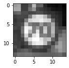
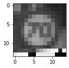
Figure 1: Randomly taken test sample (left) and transformed, sensitive sample (right)

Scaling of (2) to larger networks:

Sec. B of the Technical Appendix shows results of attempting to scale the naive approach to larger networks. Sec. C shows raw size data for various SMT encodings.

Employing Alg. 1:

We allotted 20/60/120sec as the increasing time per iteration of the for loop in Line 4, before the algorithm moves on to the next ReLU combination. This reflects the greedy character of the algorithm: we want to first try many instantiations of ReLU nodes as “identity” or “zero”, believing that one of them will give us a solution. If this approach fails, we increase the time allotment per iteration. This serves the goal of delaying advancing to later iterations, with fewer fixed ReLU nodes, as much as possible, which eventually degenerates the algorithm to one that simply has the solver explore the many ReLU combinations. In Table 1, the iteration number where a satisfying assignment was finally found is given in column “iter. #”. Small numbers here indicate success of the philosophy purported by Alg. 1. Column “runtime” shows the total time it took to find a satisfying assignment, i.e., the sum across all iterations, for a respective iteration timeout of 20/60/120sec. If a solution is found for an iteration timeout of 20sec, one would normally stop the algorithm. In order to evaluate scalability, we include results for larger time allotments. But despite the extension, the solver wounded up with the same result as with the initial allocation.

Network size	iter. #	sensitivity	SIP	total runtime (s)
30x20x10x1	6	0.1234	1.08E-05	111/312/ 612
40x20x20x1	4	0.8342	2.99E-05	65/185/ 365
50x30x10x1	14	0.3520	1.33E-05	264/784/1564
50x30x20x1	12	0.0249	4.00E-05	230/670/1330
60x40x20x1	2	0.9859	5.04E-06	36/ 75/ 135
90x60x30x1	—	—	—	(out of resources)

Table 1: Search with ReLU profiling algorithm

Comparison naive approach/Alg. 1:

Consider the case of the 30x20x10x1 NN model. Alg. 1 found a satisfying assignment in iteration #6. This means that the activation functions of five neurons—those with the smallest d-bias—were freed from their fixed instantiation to the identity or zero functions, and reverted to exact ReLU semantics. This combination yielded a sensitivity of 12.34 percentage points, a higher sensitivity than the solution found by the naive approach. The time reported for Alg. 1’s 20s/iter. run (111s) is larger though. This is not surprising, since Alg. 1 “wastes” five SMT runs. In fact, the motivation for using this algorithm is not to find solutions in “easy” cases faster. It is, instead, to increase scalability to larger models. Indeed, Alg. 1 was able to solve all models except the 90x60x30x1 case, while the naive approach timed out for most.

Presently, the method is not able to handle deeper and larger networks, such as state-of-the-art convolutional neural networks. Nevertheless, the DNN models that we presented are valid networks; we showed that SMT solvers can be used for such NN queries, e.g., sensitive-sample generation, when appropriately formalized. To deal with the complexity of DNNs, research has been conducted into dedicated theories for NN queries, e.g., Reluplex [9]. Using a dedicated solver may potentially address the scalability issue further: we first use Alg. 1 to eliminate some ReLU nodes, (e.g. the ones with high bias), while others are left in. For those left in, Reluplex can be applied. The investigation of this possibility can be picked up in future work.

6 Related Work

This work was inspired by the sensitive-sample fingerprinting technique proposed by He et al. [8], which uses classic machine learning techniques based on (projected) gradient ascent to determine sensitive samples. This is very efficient, but requires a starting point for the search and a convex solution space. Lack of convexity can lead to sub-optimality or, worse, failure to converge. The goal here was to solve a similar problem, but bring the flexibility of symbolic constraint solvers to bear: we can specify any search space and sample conditions, as long as they are definable in the underlying logic. However, definability does not imply efficient processibility, which is why Sec. 4 presents an algorithm for improved satisfiability checking.

Solving an optimization problem, the gradient-based technique returns samples that maximize the sensitivity. The authors conclude that any output discrepancy confirms the presence of an attack (“guarantee[s] zero false positives” [8]). As discussed in Sec. 3.2, this is not quite true: due to platform-dependencies of floating-point computations [7], DNN model inference is not deterministic. We address this problem using an empirical non-zero sensitivity detection threshold (Sec. 2).

Using symbolic techniques in deep learning is still a relatively young area; examples include [6, 13]. The Reluplex SMT solver [9] introduces a theory of real arithmetic extended by the ReLU function as a primitive operation. We can view our greedy Alg. 1 as an alternative dedicated way of handling ReLU nodes. A stand-alone comparison of both methods is left for future work.

Our method needs to be instantiated for different attack types (to avoid an unrealistic universal quantification over “all” adversarial models). We have focused on Trojan attacks, a survey can be found in [11]. Strategies for formalizing other types of DNN attacks are left as future work. “Fingerprinting”, using inputs characteristic of model manipulations, is one way of detecting such attacks; there are others. For instance, we can conclude the model has been compromised if, for some class, the minimal trigger that causes a misclassification is substantially smaller than for other classes and thus is likely supported by a Trojan [14]. In that approach, the defender does not need access to the trusted model or the training data. The approach is designed specifically for backdoor-style attacks relying on a trigger. Other methods perform statistical analyses, e.g., determining the probability distribution of potential triggers [4] or of prediction results under perturbations [5]. Such analyses may not be realistic in a cloud environment.

7 Summary

We revisited the technique of retrieving sensitive samples in detecting NN attacks. A previous approach solves an optimization problem, using an efficient projected gradient-based search, in order to find the optimal sensitivity [8], which faces, however, various technical preconditions and is somewhat rigid. Our approach performs the search via a symbolic constraint solver. This permits a flexible specification of desirable features of the sample. We argue that a sample need not be optimal to be effective, as long as its sensitivity is above a threshold that delineates it from innocent perturbations that can occur upon upload of the NN model to the cloud. This alternative comes with the price of efficiency, however. To address scalability, we devised a greedy algorithm that searches through all possible combinations of the ReLU node behaviors in an “easiest-first” order. This algorithm has applications in symbolic NN analysis beyond sensitive-sample search. Future work includes investigating the performance impact of using dedicated solvers for NN queries, such as Reluplex [9].

Technical Appendix

Appendix A Background

A.1 Neural Networks

A Neural Network (NN) is a parameterized, layered function that maps a vector $X$ of features from some $n$-dimensional input space to an output $y$, which may be discrete if the task is classification, or real if regression. Given parameters $W$ (a matrix of weights and biases), each layer consists of a linear function $l_{\_}i$ over the layer’s inputs and its weight parameters, and a subsequent non-linear activation function $f_{\_}i$. Function $l_{\_}i$ is a simple dot product, translated by the bias, for a fully-connected layer. The activation for inner layers is typically implemented via the rectified linear unit, defined as $\textsc{ReLU}(b)=\max\{b,0\}$. The activated values become the inputs of the next layer. The result of the final linear function, known as logit, i.e., computed at the output layer, is passed to a special activation function $\sigma$. For a binary classification task, the output activation is typically a sigmoid function; for a multi-label classification, it is a softmax function. Output $y$ is then a set of probabilities indicating which among the labels the input $X$ most likely belongs to. For a regression task, the output activation is a linear function, which yields an output over the real numbers. Thus given a network of $L$ layers, we summarize the function computed by the NN as

$y\ =\ \sigma(l_{\_}L(f_{\_}{L-1}(\ldots f_{\_}1(l_{\_}1(X,W))\ldots)))\ =\ \sigma(F(X,W)),\$

where $F$ denotes the pre-activation output, i.e., the logit value computed for input $X$.

A.2 Trojan Attack on Neural Networks

A Trojan attack on NN perturbs model parameters in order to cause a misclassification towards a target label on inputs with an embedded trigger; the modified network is said to be Trojanned. But, when the Trojanned model is presented with inputs without the trigger, the prediction is unchanged. This makes the attack hard to detect by unsuspecting users.

There are three steps to Trojan a neural network (see figure on the right, taken from [10]). The attacker is assumed to be able to modify the model parameters. First, the attacker generates a Trojan trigger, which is a snippet embedded to a test input that excites certain neurons so that the prediction is skewed towards a target masquerade. This trigger is initialized with a mask or shape. [10] suggests that the target layer from which to establish a link with the trigger is somewhere near the middle layer, wherein the neurons that are

most connected are selected.

The authors define weight connection of a neuron as the L1-norm of the weights connected to the neuron from the previous layer. The values of the initialized trigger are set by optimizing the activation values of the select neurons to intended values, supposedly large. This establishes a strong connection between the trigger and the select neurons, so that in the presence of the former the latter have strong activations, which would influence the model prediction.

After generating the trigger, the attacker stamps it to some training samples for each of the output labels, wherein the label for all these stamped samples is the target masquerade. If the attacker does not have access to the training data, they can generate the latter by model inversion. The batch of samples to be used for retraining the NN would consist of both unstamped and stamped samples. This last step of retraining the original NN Trojans the network, such that the weights are re-adjusted so that the new model predicts the target masquerade whenever the trigger is present in a test input, but predicts normally when absent, making the attack stealthy.

Appendix B Scalability of naive sample search via SMT

Using the same training data and basic network architecture, we trained larger networks, by expanding the layer sizes. We then simulated a Trojan attack on each of these. In order to assess scalability, we kept all SS parameters as set earlier. (In practice, one might determine individual SS parameters for each network.) Although we were able to transform sensitive samples in some networks, Table 2 shows the poor scaling of the naive approach to larger networks, especially where the size of the layers close to the output increases.

Network size	sensitivity	SIP	runtime
30x20x10x1	0.0744	7.41E-06	71s
40x20x20x1	—	—	(out of resources)
50x30x10x1	0.0595	8.85E-07	4
50x30x20x1	—	—	(out of resources)
60x40x20x1	—	—	(out of resources)
90x60x30x1	—	—	(out of resources)

Table 2: Sensitivities and running time for sample search without ReLU profiling

Appendix C Raw size data for encodings of various networks

To convey an idea of the raw complexity of the SMT approach, Table 3 shows various size data of the network models and the SMT encoding (2) of the SS search.

NN dimensions	# NN param.	# ReLU nodes	SMT: LOC	SMT: file size
30x20x10x1	6,751	60	7,853	354kB
40x20x20x1	9,141	80	10,363	468kB
50x30x10x1	11,701	90	12,943	592kB
50x30x20x1	12,021	100	13,333	613kB
60x40x20x1	15,101	120	16,503	770kB
90x60x30x1	25,051	180	26,753	1,284kB

Table 3: Complexity of SMT approach: NN dimensions, number of weights and biases, number of ReLU nodes, lines of code of the SMT encoding, and file size

References

- [1]
- [2] Clark Barrett, Pascal Fontaine & Cesare Tinelli (2016): The Satisfiability Modulo Theories Library (SMT-LIB). www.SMT-LIB.org.
- [3] James Bornholt: Can you train a neural network using an SMT solver? https://www.cs.utexas.edu/~bornholt/post/nnsmt.html (access May 2021).
- [4] Huili Chen, Cheng Fu, Jishen Zhao & Farinaz Koushanfar (2019): DeepInspect: A Black-box Trojan Detection and Mitigation Framework for Deep Neural Networks. In: International Joint Conference on Artificial Intelligence (IJCAI), 10.24963/ijcai.2019/647.
- [5] Yansong Gao, Change Xu, Derui Wang, Shiping Chen, Damith Chinthana Ranasinghe & Surya Nepal (2019): STRIP: a defence against trojan attacks on deep neural networks. In: Annual Computer Security Applications Conference (ACSAC), 10.1145/3359789.3359790.
- [6] Mirco Giacobbe, Thomas A. Henzinger & Mathias Lechner (2020): How Many Bits Does it Take to Quantize Your Neural Network? In: Tools and Algorithms for the Construction and Analysis of Systems (TACAS), 10.1007/978-3-030-45237-75.
- [7] Yijia Gu, Thomas Wahl, Mahsa Bayati & Miriam Leeser (2015): Behavioral Non-portability in Scientific Numeric Computing. In: International Conference on Parallel and Distributed Computing (Euro-Par), 10.1007/978-3-662-48096-043.
- [8] Zecheng He, Tianwei Zhang & Ruby B. Lee (2019): Sensitive-Sample Fingerprinting of Deep Neural Networks. In: IEEE Conference on Computer Vision and Pattern Recognition (CVPR), 10.1109/CVPR.2019.00486.
- [9] Guy Katz, Clark W. Barrett, David L. Dill, Kyle Julian & Mykel J. Kochenderfer (2017): Reluplex: An Efficient SMT Solver for Verifying Deep Neural Networks. In: Computer Aided Verification (CAV), 10.1007/978-3-319-63387-95.
- [10] Yingqi Liu, Shiqing Ma, Yousra Aafer, Wen-Chuan Lee, Juan Zhai, Weihang Wang & Xiangyu Zhang (2018): Trojaning Attack on Neural Networks. In: Network and Distributed System Security (NDSS), The Internet Society, 10.14722/ndss.2018.23291.
- [11] Yuntao Liu, Ankit Mondal, Abhishek Chakraborty, Michael Zuzak, Nina Jacobsen, Daniel Xing & Ankur Srivastava (2020): A Survey on Neural Trojans. In: 21st International Symposium on Quality Electronic Design (ISQED), 10.1109/ISQED48828.2020.9137011.
- [12] Markus Mathias, Radu Timofte, Rodrigo Benenson & Luc Van Gool (2013): Traffic sign recognition – How far are we from the solution? In: International Joint Conference on Neural Networks (IJCNN), 10.1109/IJCNN.2013.6707049.
- [13] Luca Pulina & Armando Tacchella (2012): Challenging SMT solvers to verify neural networks. AI Commun., 10.3233/AIC-2012-0525.
- [14] Bolun Wang, Yuanshun Yao, Shawn Shan, Huiying Li, Bimal Viswanath, Haitao Zheng & Ben Y. Zhao (2019): Neural Cleanse: Identifying and Mitigating Backdoor Attacks in Neural Networks. In: 2019 IEEE Symposium on Security and Privacy (S&P), 10.1109/SP.2019.00031.