Hunting $\varepsilon$: The origin and validity of quasi-steady-state reductions in enzyme kinetics

Abstract

The estimation of the kinetic parameters that regulate the speed of enzyme catalyzed reactions requires the careful design of experiments under a constrained set of conditions. Many estimates reported in the literature incorporate protocols that leverage simplified mathematical models of the reaction’s time course known as quasi-steady-state reductions. Such reductions often — but not always — emerge as the result of a singular perturbation scenario. However, the utilization of the singular perturbation reduction method requires knowledge of a dimensionless parameter, “$\varepsilon$”, that is proportional to the ratio of the reaction’s fast and slow timescales. To date, no such ratio has been determined for the intermolecular autocatalytic zymogen activation reaction, which means it remains open as to when the experimental protocols described in the literature are even capable of generating accurate estimates of pertinent kinetic parameters. Using techniques from differential equations, Fenichel theory, and center manifold theory, we derive the appropriate “$\varepsilon$” whose magnitude regulates the validity of the quasi-steady-state reduction employed in the reported experimental procedures. Although the model equations are two-dimensional, the fast/slow dynamics are rich. The phase plane exhibits a dynamic transcritical bifurcation point in a particular singular limit. The existence of such a bifurcation is relevant, because the critical manifold losses normal hyperbolicity and classical Fenichel theory is inapplicable. We show that while there exists a faux Canard that passes directly through this bifurcation point, trajectories emanating from experimental initial conditions are actually bounded away from the bifurcation point by an asymptotic distance that is proportional to the square root of the linearized system’s eigenvalue ratio. Furthermore, we show that in some cases chemical reversibility can be interpreted dynamically as an imperfection, since the presence of reversibility can destroy the bifurcation structure present in the singular limit. By extension, some of these features are also present in the phase–plane dynamics of the famous Michaelis–Menten reaction mechanism. Finally, we show that the reduction method by which QSS reductions are justified can depend on the path taken in parameter space. Specifically, we show that the standard quasi-steady-state reduction for this reaction is justifiable by center manifold theory in one limit, and via Fenichel theory in a different limit.

1 Introduction

The model equations of biochemical systems that exhibit disparate timescales can often be systematically reduced. Classical Fenichel theory [13] rigorously justifies model reduction via projection onto a slow, normally hyperbolic invariant manifold, thereby reducing the number of equations needed to capture relevant biophysical chemical events that occur over slow timescales. The extension of singular perturbation theory to systems whose critical manifolds lose normal hyperbolicity has led to our understanding of nonlinear phenomena in biological systems [4], including relaxation oscillations [31], mixed–mode oscillations [8, 23, 56], and cardiac arrhythmias [30]. However, there is another, less emphasized — but equally important — avenue for singular perturbation theory in interdisciplinary science and applied mathematics: experimental design. In chemical kinetics, reduced models that materialize from the application of Geometric Singular Perturbation Theory (GSPT) are called quasi-steady-state approximations (QSSAs), or QSS reductions. In enzyme kinetics, QSS reductions are a predominant tool in functional characterization and drug design: kinetic parameters are estimated by fitting experimental time course data to QSS reductions via nonlinear regression analysis [42, 47, 7]. In turn, the estimated kinetic parameters provide valuable information concerning the viability and efficacy of an enzyme, substrate, inhibitor, or activator in a reaction mechanism. Accordingly, GSPT plays a central role in metabolic engineering and drug design.

While the kinetic parameters of a particular reaction mechanism will be more or less invariant with respect to certain thermodynamic constraints, the QSSAs employed in experiments are approximations and, as such, will generally be invalid unless special conditions are upheld. Consequently, if we are to estimate intrinsic kinetic parameters by fitting data to QSSAs, experiments must be prepared in a way that is compatible with the validity of the QSS reduction [42].

Since the application of GSPT relies on the existence fast and slow timescales, the experimental constraint that secures the legitimacy of a QSS reduction has a direct mathematical translation: The accuracy of a QSS reduction depends on the ratio of the fast and slow timescales, $\varepsilon$, which must be small to ensure the validity of the QSS reduction. Experiments must therefore be prepared so that $0<\varepsilon\ll 1$. But, herein lies the two-fold caveat: how do we know that a QSS reduction is the result of a singular perturbation and, if it is, then what is $\varepsilon$? This question might be superfluous to the theoretician whose job is develop and expand the theory of singular perturbations. In contrast, this is the vital question posed to the interdisciplinary scientist whose objective is to use QSS reductions to extract quantitative information from experimental data.

To articulate the challenges of this problem, and profile how mathematics plays a crucial role, we have chosen to analyze the intermolecular autocatalytic zymogen activation (IAZA) mechanism, represented schematically by

$$\ce{Z+E<=>[k_{1}][k_{-1}]C->[k_{2}]2E+W},$$ (1)

where $Z$ is a zymogen, $E$ is an active enzyme, $W$ is peptide, and $k_{1},k_{2}$ and $k_{-1}$ are deterministic rate constants. The chemical mechanism (1) is essentially the autocatalytic “cousin” of the famous Michaelis–Menten reaction mechanism. As enzyme precursors (proenzymes), zymogens have numerous biochemical functions. For example, they play a critical role in protein digestion by converting pepsin to pepsinogen [1, 38], and trypsin to trypsinogen [28, 29, 50]. However, the real motivation behind our selection of the IAZA mechanism for analysis emanates from the fact that there is a generous body of experimental literature reporting on parameter estimates extracted from fitting data to reduced models [59, 14, 15]. However, the precise, theoretical qualifiers that warrant the validity of the QSS reductions employed in the experimental literature is open and unresolved. Unfortunately, this means that the accuracy of estimated parameters reported in the literature depends on, at least in part, whether or not the experiments where prepared in a way that justifies the use of the QSSA employed in the regression procedure [24].

2 The IAZA reaction mechanism

In this section we introduce the model equations of the IAZA reaction mechanism. We also give a brief review of the reduced models employed in the experimental literature, and discuss two classical QSSAs commonly attributed to GSPT and slow manifold projection.

2.1 The mass action model equations

To derive a deterministic (and finite-dimensional) model of the IAZA reaction mechanism (1), we let $z:=z(t)$, $e:=e(t)$ and $c:=c(t)$ denote the concentrations of $Z$, $E$, and $C$ respectively, and apply the law of mass action to (1). This yields the following set of nonlinear ordinary differential equations

$$\dot{z} =-k_{1}ez+k_{-1}c,$$ (2a)

$$\dot{c} =k_{1}ez-(k_{-1}+k_{2})c,$$ (2b)

$$\dot{e} =-k_{1}ez+(k_{-1}+2k_{2})c,$$ (2c)

$$\dot{w} =k_{2}c,$$ (2d)

with “$\dot{\phantom{x}}$” denoting differentiation with respect to time. The typical initial conditions used in experiments are

$$\begin{matrix}z(0)=z_{0},&&e(0)=e_{0},&&c(0)=0,&&w(0)=0,\end{matrix}$$ (3)

and, unless otherwise stated, we will assume (3) holds in the analysis that follows.

The structure of the model equations implies the existence of conservation laws. Note that equations (2a)–(2c) obey

$$\dot{z}+\dot{c}+\dot{w}=0,$$ (4)

$$\dot{e}+\dot{c}-\dot{w}=0,$$ (5)

and their sum yields an equation that is independent of $w$:

$$\dot{z}+\dot{e}+2\dot{c}=0.$$ (6)

Integrating (6) with respect to (3) yields the conservation law $z+e+2c=E_{T}$, where $E_{T}$ is sum of initial concentrations of zymogen and enzyme: $E_{T}=z_{0}+e_{0}$. Substituting $e=E_{T}-z-2c$ into (2a)–(2b) yields

$$\dot{z} =-k_{1}(E_{T}-z)z+(k_{-1}+2k_{1}z)c,$$ (7a)

$$\dot{c} =k_{1}(E_{T}-z)z-(k_{-1}+k_{2}+2k_{1}z)c,$$ (7b)

$$\dot{w} =k_{2}c.$$ (7c)

Summing together (7a)–(7c) and integrating yields the additional conservation law

$$z_{0}=z+c+w,$$ (8)

and thus we can express the mass actions equations in terms of two variables: $(z,c),(w,z)$ or $(w,c)$.

In what follows, we will occasionally refer to the parameters $K_{M},K_{S}$ and $K$, which are comprised of rate constants. The parameters $K_{M},K_{S}$, and $K$ are:

$$K_{M}:=\cfrac{k_{-1}+k_{2}}{k_{1}},\qquad K_{S}:=\cfrac{k_{-1}}{k_{1}},\qquad K:=\cfrac{k_{2}}{k_{1}}.$$ (9)

Note that $K_{M}=K_{S}+K$.

2.2 Phase plane geometry

The mass action equations in $(w,c)$ coordinates are formulated from the conservation law (8):

$$\dot{c} =k_{1}(e_{0}+w-c)(z_{0}-c-w)-(k_{-1}+k_{2})c,$$ (10a)

$$\dot{w} =k_{2}c.$$ (10b)

Note that there are three nullclines in the $(w,c)$ phase–plane, $c=0,$ and $c=h^{\pm}(w)$:

$$c=h^{-}(w) :=\cfrac{1}{2}(K_{M}+E_{T})-\cfrac{1}{2}\sqrt{(K_{M}+E_{T})^{2}-4(z_{0}-w)(e_{0}+w)},$$ (11a)

$$c=h^{+}(w) :=\cfrac{1}{2}(K_{M}+E_{T})+\cfrac{1}{2}\sqrt{(K_{M}+E_{T})^{2}-4(z_{0}-w)(e_{0}+w)}.$$ (11b)

The nullcline $c=h^{-}(w)$ intersects with $c=0$ at the points

$$x^{(1)}=(z_{0},0),\quad x^{(2)}=(-e_{0},0).$$ (12)

Linearization reveals that $x^{(1)}$ is an attracting equilibrium point and $x^{(2)}$ is a saddle point (see Figure 1).

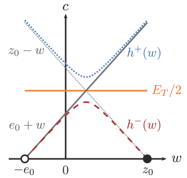
Figure 1: The phase plane geometry associated with the IAZA reaction mechanism (1) contains two equilibrium points. The dashed red curve is the $c$-nullcline given by $c=h^{-}(w)$, and the dotted blue curve corresponds to $c=h^{+}(w)$. The horizontal orange line is the constant $c=E_{T}/2$. The gray diagonal dotted line is $c=z_{0}-w$, and the gray diagonal solid line is $c=w+e_{0}$. The $c$-nullcline coincides with the $w$-axis at two equilibrium points. The black circle is the attracting equilibrium point $x^{(1)}$, located at $(z_{0},0)$ and the saddle equilibrium $x^{(2)}$ is located at $(-e_{0},0)$ and marked by a white circle.

When typical initial conditions for experiments (3) are imposed, the nullcline given by $c=h^{-}(w)$ provides an upper bound on the complex concentration, $c$. There are two cases we must work out. The first case we consider is $e_{0}\leq z_{0}$. In this scenario, the complex concentration has a maximum given by the apex of the curve $c=h^{-}(w)$. Differentiating this expression with respect to $w$ yields a critical point at $w=(z_{0}-e_{0})/2\equiv w_{T}$, and thus $\max c\leq\lambda_{Z}:=h^{-}(w_{T})$ (see Figure 2, left panel).

In contrast, if $z_{0}<e_{0}$, then the critical point at $w_{T}$ is negative, and therefore nonphysical. Thus, when experimental initial conditions are prescribed and $z_{0}<e_{0}$, the supremum of $c$ is given by $h^{-}(0)$, since $c=h^{-}(w)$ is a monotonically decreasing function on the interval $0\leq w\leq z_{0}$ (see Figure 2, right panel).

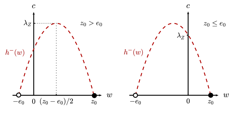
Figure 2: The supremum of $\mathbf{c}$ depends on the initial ratio of enzyme to zymogen concentration in the IAZA reaction mechanism (1). In both panels, the dashed, red curve is the $c$-nullcline given by $c=h^{-}(w)$. Left: This is an illustration of the phase plane when $e_{0}<z_{0}$. In this case, the apex of the nullcline given by $c=h^{-}(w)$ occurs at $w_{T}=(z_{0}-e_{0})/2$, which is positive. Consequently, the complex concentration is bounded by $c\leq\lambda_{Z}=h^{-}(w_{T})$. Right: In this illustration, the initial enzyme concentration is greater than the initial zymogen concentration, i.e., $z_{0}<e_{0}$. The apex of the $c$-nullcline now lies in quadrant II, and corresponds to a negative and unphysical $w_{T}$. Consequently, $c$ is bounded above by $h^{-}(0)$ when $z_{0}<e_{0}$.

From this point forward, we will simply refer to the maximum of $c$ as $\lambda_{Z}$, and take this to be $h^{-}(w_{T})$ if $e_{0}\leq z_{0}$, or $h^{-}(0)$ if $z_{0}<e_{0}$.

Note that due to conservation, any trajectory that starts inside or on the region “$\Lambda$” bounded by the curves

$$\Lambda:=\{(w,c)\in\mathbb{R}_{\geq 0}^{2}:c\leq E_{T}/2\}\cap\{(w,c)\in\mathbb{R}_{\geq 0}^{2}:c\leq e_{0}+w\}\cap\{(w,c)\in\mathbb{R}_{\geq 0}^{2}:c\leq z_{0}-w\}$$ (13)

must stay on the boundary or inside $\Lambda$ for all positive time. Thus, $\Lambda$ is positively invariant. Moreover, we can be even more restrictive, and define $\Lambda^{*}$ to be

$$\Lambda^{*}:=\Lambda\cap\{(c,w)\in\mathbb{R}^{2}_{\geq 0}:c\leq\lambda_{Z}\},$$ (14)

which is also positively invariant (see Figure 3 for an illustration of $\Lambda^{*}$).

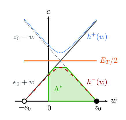
Figure 3: Due to the presence of conservation laws and attractors, the phase plane contains forward invariant sets in the IAZA reaction mechanism (1). The set $\Lambda^{*}$ is filled with green shade and outlined by the green lines. Any trajectory that starts on or in the $\Lambda^{*}$ stays on or in it for all $t>0$.

2.3 Strategies for model reduction: A brief literature review

Although the complete system (2a)–(2d) is expressible in terms of only two variables, there is a two-part question that we need to answer: Is it possible to reduce the system (7a)–(7c) further and, if so, how favorable is such a reduction with respect to a range of parameters? The answer to this question is critical for the derivation of approximate mathematical models that are more favorable (well-suited) for estimating the pertinent kinetic parameters (i.e., rate constants). Several authors attempted to address this very question. An early attempt to construct a reduced model for the IAZA reaction was made by García-Moreno et al. [15]. These authors generated what is known as a pseudo-first-order (PFO) approximation, and assumed that if $e_{0}\ll z_{0}$, then $z\approx z_{0}$ during the initial phase of the reaction. Replacing $z$ with $z_{0}$ in (7a)–(7c) results in a set of linear equations that can be easily be solved. Unfortunately, there is a downside to the PFO approach: the approximation is only valid (if at all) at the onset of the reaction, and therefore its accuracy is limited to very short (brief) timescales. Nevertheless, and despite the limitations of the linear approximation that arises from the PFO procedure, the analysis conducted in García-Moreno et al. [15] was essentially the first study in which considerable progress was made towards our understanding of autocatalytic zymogen activation reaction kinetics, since prior to the work of García-Moreno et al. [15], mostly “over-simplified” reaction mechanisms describing zymogen activation were studied [48, 49]. Later investigations [14, 55, 54] added complexity to the IAZA reaction mechanism (1), but the kinetic analyses conducted in these studies employed the basic PFO methodology of García-Moreno et al. [15].

A slightly different and more rigorous approach was developed by Wu et al. [59]. Instead of constructing a reduced model by assuming PFO kinetics, Wu et al. [59] derived a simplified model by employing a QSSA that presumes the complex concentration, $c$, changes very slowly ($\dot{c}\approx 0)$ for the majority of the reaction. By leveraging their reduced model based on the QSSA, Wu et al. [59] developed an experimental protocol and found that their estimated parameter values were close to those obtained in an earlier study by García-Moreno et al. [15]. Additional studies utilized the protocol of [59] to estimate kinetic parameters for ligand-induced autocatalytic reactions [33], and autocatalytic reactions that contain competitive inhibitors [57]. However, despite the promising results that emerged from the work of Wu et al. [59], the authors did not establish a suitable qualifier that guarantees the validity of their QSSA. Thus, it is impossible to determine the appropriate bounds within which their protocol for estimating kinetic parameters is reliable.

2.4 The classical QSS reductions of the IAZA reaction

As we mentioned earlier, QSS reductions in enzyme kinetics are based on the assumption that the reaction will undergo an initial transient phase in which the complex concentration accumulates rapidly, followed by a QSS phase where the rate of change in complex concentration nearly vanishes. The assumption that $\dot{c}$ is nearly zero provides a heuristic avenue for model reduction. Solving the equation $k_{1}(E_{T}-z)z-(k_{-1}+k_{2}+2k_{1}z)c=0$ for $c$ yields

$$c=\cfrac{(E_{T}-z)z}{K_{M}+2z},$$ (15)

and insertion of (15) into (7a) generates the classical QSS reduction for $z$:

$$\dot{z}=-\cfrac{k_{2}}{K_{M}+2z}(E_{T}-z)z.$$ (16)

Similarly, in $(c,w)$ coordinates, we take $c=h^{-}(w)$, which yields the another type of QSS reduction for $w$, which is equivalent to the reduction employed by Wu et al. [59]:

$$\dot{w}=k_{2}h^{-}(w).$$ (17)

Since the QSS phase of the reaction is valid on the slow timescale, the reductions (16) and (17) are generally assumed to hold for the majority of the reaction, and kinetic parameters are estimated by fitting (16) or (17) to experimental time course data; see Wu et al. [59] as an example that deals explicitly with the IAZA mechanism. For a more general discussion of mathematical estimation strategies, we invite the reader to consult [47, 7].

As previously stated, the classical reductions (16) and (17) are generally valid when there is an initial transient in which $c$ accumulates rapidly, followed by QSS phase in which $\dot{c}$ is very small. The fast and slow timescales measure the approximate duration of each phase and, while calculating classical QSS reductions is rather straightforward, difficulty generally emerges in the quest to justify (16) and (17). Ultimately, justification of (16) or (17) is the crux of the problem, especially if the objective is to prepare an experiment so that (16) or (17) is valid. The overwhelming tendency is to attribute the validity of an accurate QSS reduction to a singular perturbation scenario via scaling analysis. The motivation is that the qualifier (i.e., the timescale ratio “$\varepsilon$”) whose smallness justifies the QSS reduction usually emerges quite naturally from the scaled equations [25, 44]. However, the difficulty is that good scaling relies on accurate timescale estimates [44, 45]. Reliable and tractable timescale estimates can be difficult to obtain and, even if the scaling analysis suggests a singular perturbation scenario in which the theorems of Tikhonov [51] and Fenichel [13] appear to apply, the validity of a QSSA may not actually be the result of a singular perturbation scenario. As an example, we invite the reader to consult [39, 35, 20, 12], as well as [18], Section 4, for a discussion on scaling analysis. This begs the question: Is there a diagnostic methodology capable of determining when QSS reduction is the result of a singular perturbation? This answer to this question is yes, and the specific methodology that helps to delineate the applicability of Fenichel theory, referred to a Tikhonov–Fenichel Parameter Value (TFPV) theory, was recently developed by Goeke et al. [20]. We give a brief overview of TFPV theory in Section 3.

3 Application of the geometric singular perturbation theory and Tikhonov–Fenichel parameter values

Our motivation is to generate QSS reductions for the IAZA reaction mechanism from GSPT. While GSPT is certainly not the only reduction method one can employ to derive QSS reductions, it is favorable since it ensures the existence disparate fast and slow timescales. From an experimental vantage point the presence of fast and slow timescales is advantageous: the transient window that precedes the QSS phase will be short in comparison to the duration of the reaction, which means the QSSA will be valid for practically the entire time course, thereby ensuring a large window from which to extract functional data from experiments.

In this section, we review the basics of GSPT for systems that are not in standard fast/slow form. While these results are well-established, they are not as prevalent in the literature. Our outline primarily follows [58], Chapter 3. For further details, we invite the reader to consult [13, 18, 17]. We also give an overview of the more recent TFPV theory developed by Goeke et al. [20], which establishes criteria for the applicability of GSPT for enzymatic reactions. We conclude with a brief discussion on the missing piece of TFPV theory, and the open question that needs resolution.

3.1 Geometric Singular Perturbation Theory

To calculate QSS reductions we will employ GSPT. For a perturbed dynamical system of the form

$$\dot{x}=H(x)=h(x)+\varepsilon G(x,\varepsilon),\qquad x\in\mathbb{R}^{n},\quad h:\mathbb{R}^{n}\mapsto\mathbb{R}^{n},\quad G:\mathbb{R}^{n}\times\mathbb{R}\mapsto\mathbb{R}^{n},\quad 0<\varepsilon\ll 1,$$ (18)

the direct application of GSPT requires the existence of a normally hyperbolic, connected, and differentiable manifold of non-isolated stationary points, $M$, in the singular limit that corresponds to $\varepsilon=0$:

$$M:=\{x\in\mathbb{R}^{n}:h(x)=\mathbb{O}^{n}\},\qquad\dim M=k,\quad k<n.$$ (19)

The manifold $M$ is called the critical manifold. For $x\in M$, the $k$ zero-eigenvalues of $Dh(x)$ are referred to as trivial eigenvalues, and the remaining $n-k$ eigenvalues are called the non-trivial eigenvalues. Unless otherwise stated, we will assume that the real parts of the nontrivial eigenvalues are strictly less than zero, so that $M$ is attracting. Furthermore, the tangent space of $M$ at $x$, $T_{x}M$, is given by the kernel of $Dh(x)$:

$$T_{x}M=\ker Dh(x).$$ (20)

Fenichel theory applies exclusively to compact subsets, $M_{0}$, of $M$: $M_{0}\subset M$. Normal hyperbolicity ensures the existence of the splitting,

$$\mathbb{R}^{n}=T_{x}M_{0}\oplus N_{x},\qquad\forall x\in M_{0},$$ (21)

where the subspace $N_{x}$ in (21) is identically the range of $Dh(x)$ and complementary to $T_{x}M$. This structure implies the existence of a projection operator, $\Pi^{M}$,

$$\Pi^{M}:\mathbb{R}^{n}\mapsto T_{x}M_{0},$$ (22)

and the leading order QSS reduction is obtained by projecting the perturbation, $\varepsilon G(x,0)$, onto the tangent space of $M_{0}$:

$$\dot{x}=\Pi^{M}G(x,0)|_{x\in M_{0}}.$$ (23)

To construct $\Pi^{M}$, one employs the factorization $h(x)=N(x)f(x)$, where the zero level set of $f(x)$ corresponds to $M$, the columns of $N(x)$ for a basis for the range of $Dh(x)$, and the row vectors of $Df(x)$ form a basis for the orthogonal complement of $\ker Dh(x)$:

$$\text{column space}\;N=\text{range}\;Dh(x),\qquad\text{column space}\;Df^{T}=\ker^{\perp}Dh(x),\qquad\forall x\in M_{0}.$$ (24)

It follows directly from (24) that

$$\Pi^{M}:=\mathbb{I}^{n\times n}-N(DfN)^{-1}Df,$$ (25)

where $\mathbb{I}^{n\times n}$ denotes the $n\times n$ identity matrix.

As a final remark, we note that the application of GSPT is usually carried out when the perturbed dynamical system is in standard form. For a fast/slow system in $\mathbb{R}^{2}$, the standard form is:

$$\begin{bmatrix}\dot{x}\\ \dot{y}\end{bmatrix}=\begin{bmatrix}0\\ h(x,y)\end{bmatrix}+\varepsilon\begin{bmatrix}g_{1}(x,y,\varepsilon)\\ g_{2}(x,y,\varepsilon)\end{bmatrix}.$$ (26)

In this special case, we have

$$Nf=\begin{bmatrix}0\\ 1\end{bmatrix}h(x,y),\quad Df\equiv[D_{x}h\;\;D_{y}h],\quad\Pi^{M}:=\begin{bmatrix}1&0\\ -(D_{y}h)^{-1}(D_{x}h)&0\end{bmatrix},$$ (27)

and the QSS reduction is given by

$$\begin{bmatrix}\dot{x}\\ \dot{y}\end{bmatrix}=\begin{bmatrix}g_{1}(x,y,0)\\ -(D_{y}h)^{-1}(D_{x}h)g_{1}(x,y,0)\end{bmatrix}.$$ (28)

Normal hyperbolicity, $D_{y}h\neq 0$, ensures — by the Implicit Function Theorem — that $M_{0}$ is locally expressible as a graph over the slow variable, $x$: $y=X(x)$ with $h(x,X(x))=0$, and the QSS reduction in standard form is

$$\dot{x}=g_{1}(x,X(x),0).$$ (29)

Often a coordinate transformation can be utilized to recover the standard form (see [58], Section 3.7, Lemma 3.5), and well-established results in enzyme kinetics have made use of the standard form. However, the standard form in the applied literature is generally recovered not via coordinate transformation but via scaling and non-dimensionalization of the mass-action system [45]. The problem with any scaling procedure is that dimensionless variables are not unique and, despite the narrative established by several classic papers on singular perturbation analysis in enzyme kinetics [25, 44], the standard form appears to be the exception, not the rule.

3.2 Tikhonov-Fenichel Parameter Values

As noted in the previous subsection, singularly perturbed mass action systems in enzyme kinetics are not generally in standard form. Furthermore, valid QSS reductions are not necessarily the result of a singular perturbation scenario [12, 20, 39, 35]. This is not at all obvious. Goeke et al. [19, 20] and Goeke [16] were the first to make note of that QSS reductions are not necessarily the result of a singular perturbation in their development of TFPV theory. The insight of Goeke et al. [19, 20] and Goeke [16] was to recognize that if a QSS reduction is the result of a singular perturbation scenario, then there must exist a normally hyperbolic critical manifold in the singular limit. Simply stated, a TFPV is a point in parameter space at which the mass action system is equipped with a normally hyperbolic critical manifold of non-isolated equilibrium points.

The IAZA reaction is equipped with a four-dimensional parameter space, $\pi:=[k_{1}\;k_{2}\;k_{-1}\;E_{T}]^{T}$. Within this parameter space there are two TFPVs of significant interest:

$$\pi_{1}^{\star} :=[0\;k_{2}\;k_{-1}\;E_{T}],$$ (30a)

$$\pi_{2}^{\star} :=[k_{1}\;0\;k_{-1}\;E_{T}].$$ (30b)

The one-dimensional critical manifold associated with $\pi_{1}^{\star}$ is the $z$-axis ($c=0$): $M_{0}:=\{((z,c)\in\mathbb{R}^{2}_{\geq 0}:c=0\}$. It is straightforward to verify that $M_{0}$ is normally hyperbolic, and thus the decomposition (21) holds for all $(z,0)\in M_{0}\cap\Lambda$.

To calculate the QSS reduction that corresponds to small $k_{1}$, we map $k_{1}\mapsto\varepsilon k_{1}^{\star}$, and rewrite the mass action equations as

$$\dot{z} =-\varepsilon k_{1}^{\star}(E_{T}-z)z+(k_{-1}+2\varepsilon k_{1}^{\star}z)c,$$ (31a)

$$\dot{c} =\;\;\varepsilon k_{1}^{\star}(E_{T}-z)z-(k_{-1}+k_{2}+2\varepsilon k_{1}^{\star}z)c.$$ (31b)

With $0<\varepsilon\ll 1$ and $k_{1}^{\star}$ carrying unit dimension, we express the system (31) in singular perturbation form:

$$\begin{bmatrix}\dot{z}\\ \dot{c}\end{bmatrix}=\begin{bmatrix}k_{-1}\\ -(k_{-1}+k_{2})\end{bmatrix}c+\varepsilon\begin{bmatrix}-k_{1}^{\star}(E_{T}-z)z+k_{1}^{\star}zc\\ \;\;k_{1}^{\star}(E_{T}-z)z-k_{1}^{\star}zc\end{bmatrix}.$$ (32)

By inspection of (32), we identify the following:

$$N:=\begin{bmatrix}k_{-1}\\ -(k_{-1}+k_{2})\end{bmatrix},\quad f:=c,\quad Df:=[0\;1],\quad G(z,c,0):=\begin{bmatrix}-k_{1}^{\star}(E_{T}-z)z+k_{1}^{\star}zc\\ \;\;k_{1}^{\star}(E_{T}-z)z-k_{1}^{\star}zc\end{bmatrix}.$$ (33)

From (33) the projection matrix and associated QSS reduction are both straightforward to calculate,

$$\Pi^{M}:=\begin{bmatrix}1&\cfrac{K_{S}}{K_{M}}\\ 0&0\end{bmatrix},\qquad\begin{bmatrix}\dot{z}\\ \dot{c}\end{bmatrix}=\Pi^{M}G(z,0,0)=\begin{bmatrix}-\cfrac{k_{1}^{\star}k_{2}}{k_{-1}+k_{2}}(E_{T}-z)z\\ 0\end{bmatrix}.$$ (34)

Thus, in the limit as $k_{1}\to 0$, the QSS reduction for $z$ is given by

$$\dot{z}=-\cfrac{k_{2}}{K_{M}}(E_{T}-z)z,$$ (35)

and from this point forward will refer (35) as the standard QSS approximation for $z$.

Remark 1.

Note that the QSS reduction (35) is different than the classical reduction given by (16). However, they are asymptotically equal in the limit of small $k_{1}$. Goeke et al. [20] presents a thorough discussion on the asymptotic relationship between classical and Fenichel reduction.

A similar calculation can be performed for $\pi^{\star}_{2}$ by mapping $k_{2}\mapsto\varepsilon k_{2}^{\star}$ and repeating the same procedure. We will omit the details and simply state the result (see Appendix for further details). In the limit as $k_{2}\to 0$ with all other parameters bounded away from zero, the corresponding QSS reduction is

$$\dot{z}=-\cfrac{k_{2}z(E_{T}-z)(K_{S}+2z)}{K_{S}^{2}+(E_{T}+2z)K_{S}+2z^{2}},\quad K_{S}=k_{-1}/k_{1},$$ (36)

and from this point forward we refer to (36) as the QSS approximation for $z$ when $w$ is slow.

Alternatively, in $(w,c)$–coordinates the system

$$\dot{c} =k_{1}(e_{0}+w-c)(z_{0}-c-w)-(k_{-1}+\varepsilon k_{2}^{\star})c$$ (37a)

$$\dot{w} =\varepsilon k_{2}^{\star}c$$ (37b)

is in standard form when $k_{2}$ is small, and the QSS reduction for $w$ is

$$\dot{w}=k_{2}h^{-}(w;K_{S}),$$ (38)

where “$h^{-}(w;K_{S})$” in (38) is understood to mean that $K_{M}$ is replaced with $K_{S}$ in the expression for $h^{-}(w)$.

What remains is to quantify the approach to the QSS. This can be done by analyzing the layer problem, obtained by setting $\varepsilon=0$ in (31). For $k_{1}=0$, the relationship

$$z-z_{0}=\cfrac{K_{S}}{K_{M}}(c-c(0))$$ (39)

holds in the approach to the critical manifold. Thus, if $c(0)=0$, then the initial condition for the reduced problem is $z_{0}$, which agrees with the classical reduction. Consequently, the initial value problem

$$\dot{z}=-\cfrac{k_{2}}{K_{M}}(E_{T}-z)z,\quad z(0)=z_{0},$$ (40)

is the leading order approximation for $z$ for small $k_{1}$. Furthermore, integration of (40) yields closed-form solutions for $z$ and $w$:

$$z(t) =\cfrac{z_{0}E_{T}}{e_{0}\exp[{\displaystyle k_{2}\,E_{T}t/K_{M}}]+z_{0}},$$ (41a)

$$w(t) =z_{0}-z(t).$$ (41b)

When $k_{2}=0$, $w$ is conserved in the approach to the critical manifold, and $z+c=z_{0}+c_{0}$. If $c_{0}=0$, then $z=z_{0}-\lambda_{Z}$ at the onset of the QSS. Consequently, the initial value problems

$$\dot{z} =-\cfrac{k_{2}z(E_{T}-z)(K_{S}+2z)}{K_{S}^{2}+(E_{T}+2z)K_{S}+2z^{2}},\quad z(0)=z_{0}-\lambda_{Z},$$ (42a)

$$\dot{w} =k_{2}h^{-}(w;K_{S}),\qquad\qquad\qquad\quad\;\;w(0)=0,$$ (42b)

respectively approximate $z$ and $w$ during the QSS phase of the reaction. Note that $z(0)$ for (42) may be much less than $z_{0}$.

3.3 The missing piece of the puzzle: what is $\varepsilon$?

The TFPV theory developed by Goeke et al. [19, 20] provides a direct method for obtaining QSS reductions that emerge as a result Fenichel theory and a singular perturbation scenario. Hence, it partially answers the origin problem of: where do QSS reductions come from? However, the entire story in incomplete on least three counts. First, the notion of “small” is, at this juncture, somewhat abstract and not very quantitative. The answer to the question “How small must $k_{1}$ be so that (35) provides a reliable approximation to the full system (7a)-(7c)?” is unclear at this point, since the term small is relative: a concentration is only small in comparison to another, larger concentration; a rate constant is small only in comparison to some other, larger, rate constant. The answer to the question pertaining to the magnitude of a perturbation to the TFPV is important, especially if the objective is to prepare an experiment in a way that ensures (35) is accurate. Ultimately, if one one wishes to employ (35) to estimate kinetic data from an assay, then it is necessary that $\pi$ be very close to $\pi_{1}^{\star}$. But, any notion of “close” remains undefined at this juncture.

Second, GSPT is not the only method capable of generating reduced models. As we already mentioned, QSS parameters defined by Goeke et al. [20] establish a clear criterion for the near-invariance of the QSS manifold, and near-invariance is often sufficient to validate a QSS reduction [12]. Hence, not all reductions originate from a “singular perturbation scenario”. In addition to Fenichel reduction, center manifold reduction is another popular technique [6, 22]. The center manifold method is similar to Fenichel reduction in that the former reduces the full model via projection onto a low-dimensional invariant manifold (the center manifold). However, center manifold reduction and Fenichel reduction are not the same: center manifold reduction requires the existence of one non-hyperbolic equilibrium point, whereas Fenichel reduction requires a normally hyperbolic critical manifold, comprised of an infinite number of equilibria. Since TFPV theory establishes criteria for the applicability of Fenichel reduction, it is possible that other reductions may exist, and may not originate from a singular perturbation but a center manifold scenario (i.e., at a point in parameter space where a stationary point in the phase–plane becomes non-hyperbolic).

Third, TFPV theory assumes, by definition, that the critical manifold is normally hyperbolic everywhere. This is somewhat restrictive, since in most applications one must deal with points where

$$\text{rank}\;DfN|_{x\in M_{0}}<n-k.$$ (43)

In the model equations of the IAZA reaction mechanism, the loss of normal hyperbolicity occurs in the critical set that materializes when

$$\pi=\pi^{\ddagger}:=[k_{1}\;0\;0\;E_{T}].$$ (44)

In $(w,c)$-space, the critical set, $\mathcal{S}_{0}$, that emerges when $\pi=\pi^{\ddagger}$ is

$$\mathcal{S}_{0}:=\mathcal{S}_{1}\cup\mathcal{S}_{2}=\{(w,c)\in\mathbb{R}^{2}_{\geq 0}:c=z_{0}-w\}\cup\{(w,c)\in\mathbb{R}^{2}_{\geq 0}:c=e_{0}+w\}.$$ (45)

If $z_{0}>e_{0}$, then the sets $\mathcal{S}_{1}$ and $\mathcal{S}_{2}$ intersect in the first quadrant at the point $(w,c)=(w_{T},E_{T}/2)$, and the splitting (21) does not hold. Fortunately, the loss of normal hyperbolicity does not mean we cannot construct a QSS reduction; it simply means we must exercise caution in the neighborhood of $\mathcal{S}_{1}\cap\mathcal{S}_{2}$. As we will show later on, near the singular limit corresponding to $\pi^{\ddagger}$, typical trajectories initially follow $\mathcal{S}_{2}$ but later follow $\mathcal{S}_{1}$ for the remainder of the reaction. Thus, the qualitative behavior of the system is obvious. The problem emerges when we try to make quantitative statements about the efficacy of the QSS reduction near the singular point at $\mathcal{S}_{1}\cap\mathcal{S}_{2}$. It is well-established from Fenichel theory that a small perturbation to the vector field $h(x)$ results in the birth of an invariant slow manifold, $M_{\varepsilon}$, whose Hausdorff distance, $d_{H}$, is $\mathcal{O}(\varepsilon)$ from $M_{0}$ (see [32], Chapters 2-3, for a clear presentation of general Fenichel theory and its application to fast/slow dynamical systems), which is a quantitative statement concerning the asymptotic validity of the QSS reduction. Since classical Fenichel theory breaks down at $\mathcal{S}_{1}\cap\mathcal{S}_{2}$, the integrity of a QSS reduction in the vicinity of this point is unclear.

4 Unveiling $\varepsilon$: Dimensionless singular perturbation parameters

In this section we provide an answer to the question: How small must a TFPV in order to ensure the associated QSS reduction is reliable? A direct approach involving the eigenspectrum of championed by Palsson and Lightfoot [36] ensures the eigenvalue ratio of $DH(x)$ at the unique equilibrium point is small. However, this approach seems rather limited for two reasons. First, the layer problem with $\varepsilon=0$ contains an infinite number of equilibrium points, and thus estimating the spectral gap at just one of the equilibria may, in some cases, be an oversimplification. Second, the eigenspectrum of the Jacobian can completely vanish at points where the critical manifold fails to be normally hyperbolic, and linear methods do not suffice in such situations.

The more general approach that we take leverages the phase plane geometry of the IAZA reaction. We begin with the preliminary assumption that

$$c=h^{-}(w)+\mathcal{E}_{Z},$$ (46)

where $\mathcal{E}_{Z}$ is an error term. The motivation behind this choice is that the QSS manifold approaches the critical manifold(s) in the singular limits discussed in Section 3. The objective is then to establish criteria that ensures $\mathcal{E}_{Z}$ is small. To generate the condition(s) that render $\mathcal{E}_{Z}$ negligible, we compute the limit supremum

$$\limsup_{t\to\infty}\;\mathcal{E}_{Z}^{2}\leq\varepsilon^{2}\lambda_{Z}^{2}.$$ (47)

The relationship between $e_{0}$ and $z_{0}$ alters the value of $\lambda_{Z}$ according to the phase plane geometry described in Section 2. As a reminder, $\lambda_{Z}$ is given by

$$\max c:=\lambda_{Z}=\begin{cases}h^{-}((z_{0}-e_{0})/2)&\text{if}\quad e_{0}<z_{0},\\ h^{-}(0)&\text{if}\quad z_{0}\leq e_{0}.\end{cases}$$

Let us next define

$$\mu:=\sqrt{(K_{M}+E_{T})^{2}-4e_{0}z_{0}}\quad\text{ and }\gamma:=\sqrt{K_{M}(K_{M}+2E_{T})},$$

so $\lambda_{Z}$ can be written as

$$\lambda_{Z}=\begin{cases}\big{(}K_{M}+E_{T}-\gamma\big{)}\big{/}2&\text{if}\quad e_{0}<z_{0},\vspace{1mm}\\ \big{(}K_{M}+E_{T}-\mu\big{)}\big{/}2&\text{if}\quad z_{0}\leq e_{0}.\\ \end{cases}$$

The derivative of $\mathcal{E}_{Z}^{2}$ is:

$$\cfrac{1}{2}\cfrac{\text{d}\mathcal{E}_{Z}^{2}}{\text{d}t} =[\dot{c}-D_{w}h^{-}(w)\dot{w}]\mathcal{E}_{Z}$$ (48a)

$$=[k_{1}(c-h^{+}(w))(c-h^{-}(w))-D_{w}h^{-}(w)\dot{w}]\mathcal{E}_{Z}.$$ (48b)

Phase plane geometry dictates that $c-h^{+}(w)<0$ for any trajectory starting in or on $\Lambda^{*}$. It follows from (48) that

$$\cfrac{1}{2}\cfrac{\text{d}\mathcal{E}_{Z}^{2}}{\text{d}t}\leq k_{1}\max[c-h^{+}(w)]\mathcal{E}_{Z}^{2}+\max|D_{w}h^{-}(w)|\max|\dot{w}||\mathcal{E}_{Z}|.$$ (49)

Remark 2.

We have exploited the fact that the derivative function for $\dot{c}$ factors as $\dot{c}=k_{1}(c-h^{-}(w))(c-h^{+}(w))$ to recover (49). It is this geometric feature, which is common in most mass actions systems that model enzyme kinetics, that allows us to generate sharp error estimates.

The term “$\max[c-h^{+}(w)]$” is easily bounded above by

$$\lambda_{Z}-\displaystyle\min_{0\leq w\leq z_{0}}h^{+}(w),$$

where $\min h^{+}(w)$ is given by

$$\min_{0\leq w\leq z_{0}}h^{+}(w)=\begin{cases}h^{+}((z_{0}-e_{0})/2)\qquad\text{if}\;\;e_{0}<z_{0},\\ h^{+}(0)\qquad\qquad\qquad\;\text{if}\;\;z_{0}\leq e_{0}.\end{cases}$$

Using definition (4), we calculate $\max[c-h^{+}(w)]$

$$\max_{c\in\Lambda^{\star}}\;[c-h^{+}(w)]:=-\varphi=\begin{cases}-\sqrt{K_{M}(K_{M}+2E_{T})}=-\gamma\qquad\qquad\;\;\;\text{if}\;\;e_{0}\leq z_{0},\\ \\ -\sqrt{(K_{M}+E_{T})^{2}-4e_{0}z_{0}}=-\mu\qquad\quad\text{if}\;\;z_{0}<e_{0}.\end{cases}$$ (50)

The last term on the right hand side of (49) is easily bounded in terms of $\mathcal{E}_{Z}^{2}$,

$$\max|D_{w}h^{-}(w)|\max|\dot{w}||\mathcal{E}_{Z}|\leq\delta\mathcal{E}_{Z}^{2}+\cfrac{(\max|D_{w}h^{-}(w)|\max|\dot{w}|)^{2}}{4\delta}.$$ (51)

Choosing $\delta=k_{1}\varphi/2$ and applying Grönwall’s lemma yields

$$\mathcal{E}_{Z}^{2} \leq\mathcal{E}(0)_{Z}^{2}e^{-\displaystyle k_{1}\varphi t}+\cfrac{(\max|D_{w}h^{-}(w)|\max|\dot{w}|)^{2}}{(k_{1}\varphi)^{2}}\bigg{(}1-e^{\displaystyle-k_{1}\varphi t}\bigg{)},$$ (52a)

$$\leq\mathcal{E}(0)_{Z}^{2}e^{-\displaystyle k_{1}\varphi t}+\cfrac{(\max|D_{w}h^{-}(w)|\max|\dot{w}|)^{2}}{(k_{1}\varphi)^{2}}.$$ (52b)

The constants that bound the $\limsup$ of $\mathcal{E}_{Z}^{2}$ are easily computed over $\Lambda^{*}$ using standard calculus techniques

$$\max_{(c,w)\in\Lambda^{*}}|D_{w}h^{-}(w)|=\cfrac{E_{T}}{K_{M}+E_{T}},\qquad\max_{(c,w)\in\Lambda^{*}}|\dot{w}|=k_{2}\lambda_{Z}.$$ (53)

Finally, from (53) and (52) we have

Proposition 1.

For every solution of with initial value in $\Lambda^{*}$ it holds that

$$\mathcal{E}_{Z}^{2}(t)\leq\mathcal{E}^{2}(0)e^{-\tau}+\varepsilon^{2}\lambda_{Z}^{2},$$ (54)

with $\tau:=k_{1}\varphi t$. Thus with

$$\varepsilon:=\bigg{(}\cfrac{E_{T}}{K_{M}+E_{T}}\bigg{)}\bigg{(}\cfrac{K}{K_{M}}\bigg{)}\bigg{(}\cfrac{K_{M}}{\varphi}\bigg{)},\quad\text{\rm with}\quad K=k_{2}/k_{1},$$ (55)

the solution approaches the QSS manifold, $c=h^{-}(w)$, up to an error of $\lambda_{Z}^{2}\varepsilon^{2}$, with time constant $\lambda_{\tau}:=k_{1}\varphi$.

Proposition 1 suggests that $\varepsilon$ defined by (55) is the singular perturbation parameter that regulates the accuracy of the classical reduction (17). This follows from the observation that a singular perturbation parameter proportional to a ratio of fast and slow timescales is dimensionless. If one non-dimensionalizes the mass action equations, then it is natural to scale $c$ by its maximum value, $\lambda_{Z}$. In this case the magnitude of the scaled error, $\lambda_{Z}^{-2}\cdot[c-h^{-}(w)]^{2}:=[\hat{c}-\hat{h}^{-}(w)]^{2}$, is regulated (asymptotically) by $\varepsilon$, and therefore one would naturally take $\varepsilon$ in Proposition 1 to be the appropriate singular perturbation parameter when the mass action equations are dimensionless.

The form of $\varepsilon$ in (55) is revealing, as it factors into three small parameters, $\varepsilon_{1}$, $\varepsilon_{2}$ and $\varepsilon_{\ddagger}$,

$$\varepsilon_{1}:=\cfrac{k_{1}E_{T}}{k_{-1}+k_{2}+k_{1}E_{T}}\leq 1,\qquad\varepsilon_{2}:=\cfrac{k_{2}}{k_{-1}+k_{2}}\leq 1,\qquad\varepsilon_{\ddagger}:=\cfrac{k_{-1}+k_{2}}{k_{1}\varphi}\leq 1.$$ (56)

Remark 3.

By inspection, it is clear that conditions $\varepsilon_{1}\ll 1$ and $\varepsilon_{2}\ll 1$ determine the validity of the standard QSS approximation for $z$ (35) and the QSS approximation for $z$ when $w$ is slow (36), respectively. This follows from the observation that $\varepsilon_{1}=0$ if $k_{1}=0$, and $\varepsilon_{2}=0$ if $k_{2}=0$, and thus the limiting cases of $\varepsilon_{1}\to 0$ and $\varepsilon_{2}\to 0$ correspond with the TFPVs $\pi_{1}^{\star}$ and $\pi_{2}^{\star}$. Thus, the dimensionless parameters $\varepsilon_{1}$ and $\varepsilon_{2}$ give us a measure of the “size” of $k_{1}$ or $k_{2}$ with respect to a perturbed $\pi_{1}^{\star}$ or $\pi_{2}^{\star}$. Numerical results support this claim; see Figures 4 and 5.

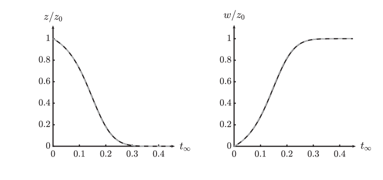
Figure 4: The sQSSA, (41a) and (41b), for the IAZA reaction mechanism (1) is valid when $\mathbf{E_{T}\ll K_{M}}$. In both panels, the solid black curve is the numerical solution to the mass action equations (7a)–(7c), and the dashed black curve (barely visible) is the numerical solution to (41a). The rate constants used to construct the numerical approximation are: $e_{0}=9$, $z0=1$, $k_{1}=2$, $k_{-1}=k_{2}=500$. Left: In this panel, the solid black curve is the numerical solution to $z(t)$, and the dashed black curve is the solution generated by (41a). Right: In this panel, the solid black curve is the numerical solution to $w(t)$, and the dashed black curve is the solution generated by (41b). For illustrative purposes, the units of all parameters and concentrations are arbitrary. Time has been mapped to the $t_{\infty}$ scale: $t_{\infty}(t)=1-1/\ln[t+\exp(1)]$.

Figure 5: The reductions (38) and (36) are valid for the IAZA reaction mechanism (1) when $\mathbf{k_{2}\ll k_{-1}}$. In all panels, the solid black curve is the numerical solutions to the mass action equations (7a)–(7c). In the upper and lower right panels, the dashed/dotted curve is the numerical solution to (36) with $z^{*}$ as the initial condition. In the top panels, the parameter values and initial conditions are $k_{1}=1.0$, $k_{-1}=5$, $k_{2}=0.01$ and $e_{0}=1$, $z_{0}=9$. In the bottom panels, the parameter values and initial conditions are $k_{1}=1.0$, $k_{-1}=5$, $k_{2}=0.01$ and $e_{0}=7$, $z_{0}=3$. For illustrative purposes, the units of all parameters and concentrations are arbitrary. In the upper and lower right panels, time has been mapped to the $t_{\infty}$-scale: $t_{\infty}(t)=1-1/\ln[t+\exp(1)]$. Top Left: This panel illustrates a typical trajectory in the $(w,c)$ phase plane when the tQSSA is valid. The dashed red curve is the $c$-nullcline $h^{-}(w)$, and by inspection it is easy to see that (38) is justified when $k_{2}\ll k_{-1}$. Top Right: In this panel, the numerical solutions to $z$ as well as (36) are compared on the $t_{\infty}$ scale. Clearly, (36) serves as a good approximation to $z(t)$. The lower left and lower right panels give analogous illustrations of the $(w,c)$ phase plane and temporal dynamics when $e_{0}\geq z_{0}$.

At this juncture, it is important to give the dimensionless parameters $\varepsilon_{1}$ and $\varepsilon_{2}$ a proper interpretation in the context of singular perturbation reduction and TFPV theory. Recall that the reduction (35) is valid — and justified from singular perturbation theory — as $k_{1}\to 0$. The question we set out to answer pertained to how small one must take $k_{1}$ in order to be confident that (35) accurately approximates the full system on the slow timescale. Let us now rephrase this question with more clarity: if all other parameters are fixed, or bounded below and above by positive constants, how small, in comparison to the other parameters, must we take $k_{1}$ to secure an accurate reduction in (35)? The answer is until $\varepsilon_{1}\ll 1$. If $E_{T}$, $k_{-1}$ and $k_{2}$ are held constant, then $k_{1}$ should be reduced in magnitude until $k_{1}$ is at least small enough that $\varepsilon_{1}\ll 1$. Loosely speaking, if one were to define a one-dimensional search direction in parameter space along $k_{1}$, with all other parameters constant, then $\varepsilon_{1}\ll 1$ can be interpreted as a stopping criterion. A similar interpretation holds for $k_{2}$, $\varepsilon_{2}$, and (36) and (42).

Note that $\varepsilon_{1}\to 0$ vanishes not only as $k_{1}\to 0$, but also as $E_{T}\to 0$. However, the latter does not result in a singular perturbation scenario, and thus one cannot attribute the accuracy of (16) to Fenichel theory. Nevertheless, Proposition 1 clearly indicates that (35) will improve as $E_{T}\to 0$, and this demands explanation. First, note that the normal form of a static transcritical bifurcation

$$\dot{x}=rx-x^{2},$$ (57)

is recovered from (35) by reparameterizing time, $\tau:=-k_{2}t/K_{M}$, and thus $E_{T}$ in (35) is equivalent to the bifurcation parameter “$r$” in the normal form (57). Moreover, setting $E_{T}=0$ in the rate equations results in the formation of a non-hyperbolic fixed point at the origin. Consequently, the origin is equipped with center manifold, $W^{c}(0)$, when $E_{T}=0$. For small $E_{T}$ and $z\in[0,z_{0}]$, the long-time dynamics can be approximated via projection onto the local center manifold, $W^{c}_{\text{loc.}}(0)$, defined in the extended phase space, $(z,c,E_{T})\in\mathbb{R}^{3}.$ To leading order, the dynamics of $z$ on the center manifold is

$$\dot{z}=-\cfrac{k_{2}}{K_{M}}(E_{T}-z)z,$$

which is equal to (35) (see Appendix for the detailed calculation). This example illustrates that the mathematical justification of the QSS reduction may be multifaceted. Ultimately, the justification depends on which path is taken in parameter space. For example, taking $k_{1}\to 0$ with all other parameters constant (and positive) results in justification from Fenichel theory. Center manifold reduction legitimizes the QSS reduction as $E_{T}\to 0$ with all other parameters positive and constant and $z\leq z_{0}<E_{T}$. Thus, while the reductions as $k_{1}\to 0$ and $E_{T}\to 0$ are the same, the origin is different.

The remaining dimensionless parameter, $\varepsilon_{\ddagger}$, vanishes when both $k_{-1}$ and $k_{2}$ vanish as long as $z_{0}<e_{0}$, which is consistent with $\pi^{\ddagger}$. However, $\pi^{\ddagger}$ is not a TFPV due to the lack of normal hyperbolicity. Nevertheless — and on an intuitive level — we expect $\varepsilon_{\ddagger}$ to tell us something about the efficacy of a QSS reduction near $\pi^{\ddagger}$. Such is the subject of Section 5.

5 The loss of normal hyperbolicity

5.1 The Layer Problem

In perturbation form, and in $(c,w)$ coordinates, the mass action system for small $k_{-1}$ and $k_{2}$ is

$$\begin{bmatrix}\dot{c}\\ \dot{w}\end{bmatrix}=\begin{bmatrix}k_{1}(e_{0}+w-c)(z_{0}-c-w)\\ 0\end{bmatrix}+\varepsilon\begin{bmatrix}-(k_{-1}^{\star}+k_{2}^{\star})\\ k_{2}^{\star}\end{bmatrix}c,$$ (58)

and is thus a fast/slow system in standard form. The layer problem corresponds to the singular limit with $\varepsilon=0$ in (58), but the critical set (45) of the layer problem is not a manifold. Moreover, normal hyperbolicity does not hold at $\mathcal{S}_{1}\cap\mathcal{S}_{2}$ located at $(w,c)=((z_{0}-e_{0})/2,E_{T}/2):=(w_{T},c_{T})$, since

$$\cfrac{\partial}{\partial c}\;k_{1}(e_{0}+w-c)(z_{0}-c-w)\bigg{|}_{(c,w)=(c_{T},w_{T})}=0.$$ (59)

However, apart from $\mathcal{S}_{1}\cap\mathcal{S}_{2}$, the stability of the additional equilibria that comprise $\mathcal{S}_{0}$ is straightforward to compute

$$\cfrac{\partial}{\partial c}\;k_{1}(e_{0}+w-c)(z_{0}-c-w)\bigg{|}_{c=z_{0}-w} =-k_{1}(e_{0}-z_{0}+2w):=\lambda_{1}(w),$$ (60a)

$$\cfrac{\partial}{\partial c}\;k_{1}(e_{0}+w-c)(z_{0}-c-w)\bigg{|}_{c=e_{0}+w} =\;\;k_{1}(e_{0}-z_{0}+2w):=\lambda_{2}(w),$$ (60b)

and from (60) a clear picture emerges:

Proposition 2.

With $\mathcal{S}_{1}:=\{(c,w)\in\mathbb{R}^{2}_{\geq 0}:c=z_{0}-w\}$, $\mathcal{S}_{2}:\{(c,w)\in\mathbb{R}^{2}_{\geq 0}:c=e_{0}+w\}$, and $\delta_{1},\delta_{2},\delta_{3},\delta_{4}>0$, the following holds:

1. If $z_{0}>e_{0}$ and $w>w_{T}$, then $\lambda_{2}(w)>0$ and $\mathcal{S}_{2}^{r}:=\{(c,w)\in\mathbb{R}_{\geq 0}^{2}\cap\mathcal{S}_{2}:w\geq w_{T}+\delta_{1}\}$ is comprised of repulsive fixed points w.r.t the layer problem given by the singular limit of (58).

2. If $z_{0}>e_{0}$ and $w>w_{T}$, then $\lambda_{1}(w)<0$ and $\mathcal{S}_{1}^{a}:=\{(c,w)\in\mathbb{R}_{\geq 0}^{2}\cap\mathcal{S}_{1}:w\geq w_{T}+\delta_{2}\}$ is comprised of attracting fixed points with respect to the layer problem given singular limit of (58).

3. If $z_{0}>e_{0}$ and $w<w_{T}$, then $\lambda_{2}(w)<0$ and $\mathcal{S}_{2}^{a}:=\{(c,w)\in\mathbb{R}_{\geq 0}^{2}\cap\mathcal{S}_{2}:w\leq w_{T}-\delta_{3}\}$ is comprised of attracting fixed points with respect to the layer problem given by the singular limit of (58).

4. If $z_{0}>e_{0}$ and $w<w_{T}$, then $\lambda_{1}(w)>0$ and $\mathcal{S}_{1}^{r}:=\{(c,w)\in\mathbb{R}_{\geq 0}^{2}\cap\mathcal{S}_{1}:w\leq w_{T}-\delta_{4}\}$ is comprised of repulsive fixed points with respect to the layer problem given by the singular limit of (58).

Thus, from Proposition 2 the geometric landscape of the layer problem is clear: the two submanifolds $\mathcal{S}_{1}$ and $\mathcal{S}_{2}$ exchange stability at their intersection (see Figure 6).

Figure 6: In the singular limit that occurs when $\mathbf{K_{M}=0}$, a dynamic transcritical bifurcation emerges in the vector field. When $k_{-1}=k_{2}=0$, the nullclines $c=h^{-}(w)$ and $c=h^{+}(w)$ coalesce with the curves $\mathcal{S}_{1}:=\{(c,w)\in\mathbb{R}^{2}_{\geq 0}:c=z_{0}-w\}$ and $\mathcal{S}_{2}:=\{(c,w)\in\mathbb{R}^{2}_{\geq 0}:c=w+e_{0}\}$. Each curve, $c=z_{0}-w$ and $c=w+e_{0}$, is comprised of stationary points. These curves intersect and exchange stability at the transcritical bifurcation point $(w,c)=((z_{0}-e_{0})/2,E_{T}/2)\equiv(w_{T},c_{T})$. Thus, $\mathcal{S}_{1}$ and $\mathcal{S}_{2}$ have stable (attracting) and unstable (repulsive) regions, $\mathcal{S}_{1}^{a},\mathcal{S}_{2}^{a}$ and $\mathcal{S}_{1}^{r},\mathcal{S}_{2}^{r}$, respectively. Dashed lines correspond to unstable equilibrium points, and solid lines correspond to stable equilibrium points.

The question that follows is: It is possible to construct a useful QSS reduction and, if so, how do we quantify its efficacy? If $e_{0}<z_{0}$, then physical solutions that originate in $\Lambda^{*}$ will follow $\mathcal{S}_{1}^{a}$ and $\mathcal{S}_{2}^{a}$, and the difficulty lies in gauging the accuracy of either the Fenichel reduction or the classical reduction (17) near the point of intersection, $\mathcal{S}_{1}\cap\mathcal{S}_{2}$ (see Figure 7).

Figure 7: Fenichel theory breaks down at $\mathcal{S}_{1}\cap\mathcal{S}_{2}$ and the accuracy of reduced models in the neighborhood of this point must be estimated. In both panels, the thick black curve is the numerical solution to the mass action system (7a)–(7c). The thick dashed red curves are $h^{\pm}(w)$. The thin dashed-dotted black line is $\mathcal{S}_{1}$, and the thin, dashed black line is $\mathcal{S}_{2}$. Parameters values (of arbitrary units) are: $e_{0}=5$, $z_{0}=10$, $k_{-1}=0.1$, $k_{2}=0.1$, and $k_{1}=10.0$.

One could resort to center manifold reduction but, the eigenspectrum at $\mathcal{S}_{1}\cap\mathcal{S}_{2}$ contains a zero eigenvalue with multiplicity two and, as noted in [26], center manifold reduction is not very useful in such scenarios. However, from a practical point of view, note that if $z_{0}<e_{0}$, then the layer problem has only one attracting branch ($\mathcal{S}_{1}$) contained entirely within the first quadrant. Thus, with $z_{0}<e_{0}$, the intersection $\mathcal{S}_{1}\cap\mathcal{S}_{2}$ lies in the second quadrant, and the reduced problem is

$$\dot{w}=k_{2}(z_{0}-w).$$ (61)

In enzyme kinetics, the linear QSS reduction (61) is the autocatalytic version of the reverse quasi-steady-state approximation (rQSSA) [45, 40, 10]. The experimental utility of the rQSSA is that the catalytic rate constant, $k_{2}$, can be estimated by fitting (through regression analysis) the exact solution of (61) to time course data [7]. Of course, one will normally want to refine experiments by taking different $z_{0}$ with fixed $e_{0}$ and compute an average over the range of $k_{2}$ estimates. Thus, to design a proper experimental protocol capable of estimating $k_{2}$, we must answer the twofold question: How small should $k_{-1}$ and $k_{2}$ be and, practically speaking, what ratios $z_{0}/e_{0}$ should be considered? As we illustrate in the subsection that follows, the answers to these questions are inexorably linked to Fenichel theory.

5.2 Investigating normal hyperbolicity in the irreversible IAZA reaction

To gain insight pertaining to the validity of (61), we will temporarily study the completely irreversible IAZA reaction, which is analogous to the Van Slyke-Cullen reaction mechanism:

$$\ce{Z+E->[k_{1}]C->[k_{2}]2E+W}.$$ (62)

In the singular limit that coincides with $k_{2}=0$, the geometry of the layer problem of (62) is unchanged (see Figure 6). Once the perturbation is “turned on” and $0<k_{2}$, a distinct invariant trajectory, $\mathcal{C}^{\varepsilon}$, emerges

$$\mathcal{C}^{\varepsilon}:=\mathcal{S}_{1}.$$ (63)

Thus, the set $\mathcal{S}_{1}$ remains invariant. Moreover, since the trajectory $\mathcal{C}^{\varepsilon}$ travels from the unstable ($\mathcal{S}_{1}^{r})$ to the stable ($\mathcal{S}_{1}^{a}$) sections of $\mathcal{S}_{1}$, one can refer to this distinguished trajectory as a faux Canard.

There are two cases we must consider in our assessment of reduced models obtained via projection onto normally hyperbolic and attracting subsets of $\mathcal{S}$: $z_{0}\leq e_{0}$ and $e_{0}<z_{0}$. We will begin with the latter. Linearizing about $x^{(1)}$ with $e_{0}=z_{0}$ yields

$$\begin{bmatrix}\dot{c}\\ \dot{w}\end{bmatrix}=DH(c,w)|_{(0,z_{0})}=\begin{bmatrix}-2e_{0}k_{1}-k_{2}&-2e_{0}k_{1}\\ k_{2}&0\end{bmatrix}\begin{bmatrix}c\\ w\end{bmatrix}.$$

The eigenvalues of $DH(0,z_{0})$ are $\lambda_{1}:=-k_{2}$ and $\lambda_{2}:=-2k_{1}e_{0}$, and the corresponding eigenvectors are

$$v_{1},v_{2}:=\begin{bmatrix}-1\\ \;\;\;1\end{bmatrix},\quad\begin{bmatrix}-2e_{0}k_{1}/k_{2}\\ 1\end{bmatrix}.$$

If $k_{2}\ll 2e_{0}k_{1}$, then $\text{span}\;v_{1}$ is the slow eigenspace. In the slow timescale, $T=k_{2}t$, the linear solution is

$$x=\beta_{1}v_{1}e^{-\displaystyle T}+\beta_{2}v_{2}e^{-\displaystyle T/\varepsilon},\qquad\varepsilon:=\lambda_{1}/\lambda_{2},\qquad x:=[c\;\;w-z_{0}]^{T},$$

where $\beta_{1}$, $\beta_{2}$ are constants. For initial conditions that are sufficiently close to $x^{(1)}$, the solution will lie almost entirely along the direction of $v_{1}$ after a time of order $T=-\varepsilon\ln\varepsilon$.

Certainly $\lambda_{1}/\lambda_{2}\ll 1$ is a necessary condition for the validity of (61). However, since the linearized solution is only valid in a small neighborhood surrounding $x^{(1)}$, it is unclear at this point if (61) holds after a timescale of order $T=-\varepsilon\ln\varepsilon$ for initial conditions that lie sufficiently far away from $x^{(1)}$. For a nonlinear fast/slow system of the form

$$x^{\prime} =f(x,y),$$ (64a)

$$\varepsilon y^{\prime} =g(x,y),$$ (64b)

with $\mathfrak{Re}(D_{y}g(x,y))<0\;\;\forall(x,y)\in M_{0}$, trajectories will reach an $\mathcal{O}(\varepsilon)$–neighborhood of the slow manifold once $T\sim-\varepsilon\ln\varepsilon$. However, due to the lack of normal hyperbolicity at $\mathcal{S}_{1}\cap\mathcal{S}_{2}$, a timescale estimate of $T\sim-\varepsilon\ln\varepsilon$ is possibly too short when $e_{0}=z_{0}$. Consequently, it is necessary to get a more global estimate on how quickly trajectories approach $\mathcal{C}^{\varepsilon}$ when $z_{0}=e_{0}$ if (61) is to be useful.

Proposition 3.

For all $(c,w)\in\Lambda$ with $z_{0}\leq e_{0}$ and $\varepsilon_{\ddagger}>0$, it holds that

$$\mathcal{Z}^{2}\leq\mathcal{Z}^{2}(0)e^{\displaystyle(\varepsilon_{\ddagger}-1)T/\varepsilon_{\ddagger}},$$

where $\mathcal{Z}^{2}:=[c-(z_{0}-w)]^{2}$ and $T=k_{2}t$.

Proof: For $z_{0}\leq e_{0}$, we have

$$\cfrac{\text{d}\mathcal{Z}^{2}}{\text{d}t} \leq-2k_{1}(e_{0}-\lambda_{Z})\mathcal{Z}^{2},$$

$$=-k_{1}(e_{0}-z_{0}+\sqrt{K^{2}+2E_{T}K}-K)\mathcal{Z}^{2},$$

$$\leq-k_{2}K^{-1}(\sqrt{K^{2}+2E_{T}K}-K)\mathcal{Z}^{2}.$$

As defined in the previous section, $K:=k_{2}/k_{1}$. Passing to the slow time, $T$, we obtain:

$$\cfrac{\text{d}\mathcal{Z}^{2}}{\text{d}T} \leq-K^{-1}(\sqrt{K^{2}+2E_{T}K}-K)\mathcal{Z}^{2},\quad T:=k_{2}t,$$

$$=(1-\varepsilon_{\ddagger}^{-1})\mathcal{Z}^{2},$$

$$=(\varepsilon_{\ddagger}-1)\varepsilon_{\ddagger}^{-1}\mathcal{Z}^{2},$$

and Grönwall’s lemma implies

$$\mathcal{Z}^{2}\leq\mathcal{Z}^{2}(0)e^{\displaystyle(\varepsilon_{\ddagger}-1)T/\varepsilon_{\ddagger}}\approx\mathcal{Z}^{2}(0)e^{\displaystyle-T/\varepsilon_{\ddagger}}\quad\text{for}\quad\varepsilon_{\ddagger}\ll 1.$$

Remark 4.

It is important to realize that $\varepsilon_{\ddagger}$ is in fact undefined when $e_{0}=z_{0}$ and $k_{-1}=k_{2}=0$. This is a result of the loss of normal hyperbolicity. However, with $k_{-1}=0$ and $k_{2}\to 0$, the limit from the right does exist (it is zero), and this is all that matters in applications since we are bounded away from the singular limit.

Proposition 3 confirms our intuition from Section 4 that $\varepsilon_{\ddagger}$ is the singular perturbation parameter that regulates the accuracy of the rQSSA when $z_{0}\leq e_{0}$. Moreover, it is important to emphasize that $\varepsilon_{\ddagger}$ is different, in an important way, from the singular perturbation parameter that emerges from scaling analysis. To see this, let $e_{0}=z_{0}$ and define $\bar{c}:=c/e_{0}$ and $\bar{w}:=w/e_{0}$. The dimensionless mass action system is

$$\varepsilon^{\star}\bar{c}^{\prime} =(1+\bar{w}-\bar{c})(1-\bar{c}-\bar{w})-\varepsilon^{\star}\bar{c},$$ (67a)

$$\bar{w}^{\prime} =\bar{c},$$ (67b)

where “$\phantom{x}{}^{\prime}$” denotes differentiation with respect to the slow time, $T$, and $\varepsilon^{\star}:=k_{2}/k_{1}e_{0}$. However, $\varepsilon^{\star}$ is not asymptotically equivalent to $\varepsilon_{\ddagger}$ when $z_{0}=e_{0}$. In fact, with $e_{0}=z_{0}$, and $E_{T}=2e_{0}$ we have

$$\varepsilon_{\ddagger}\approx\cfrac{1}{2}\sqrt{\varepsilon^{\star}}\sim\mathcal{O}(\sqrt{\varepsilon^{\star}})\quad\text{for}\quad k_{2}\ll k_{1}e_{0}.$$ (68)

The relationship between $\varepsilon^{\star}$ and $\varepsilon_{\ddagger}$ given by (68) allows us to better estimate the time it takes for a phase plane trajectory that starts at an $\mathcal{O}(1)$ distance from the slow manifold to reach an $\mathcal{O}(\varepsilon^{\star})$–neighborhood of the slow manifold:

$$|\bar{c}-(1-\bar{w})|\approx e^{\displaystyle-T/2\varepsilon_{\ddagger}}\approx e^{\displaystyle-T/\sqrt{\varepsilon^{\star}}}.$$ (69)

We see from (69) that the dimensionless system (67a) may require a time that is possibly closer to the order $T\sim-\sqrt{\varepsilon^{\star}}\ln\varepsilon^{\star}$ before the trajectory is $\mathcal{O}(\varepsilon^{\star})$ from the slow manifold. In addition, Proposition 3 indicates that after a time of roughly,

$$T\sim-\varepsilon_{\ddagger}\ln\varepsilon_{\ddagger},$$ (70)

the trajectory should be within an $\mathcal{O}(\varepsilon_{\ddagger})\sim\mathcal{O}(\sqrt{\varepsilon^{\star}})$–neighborhood of the slow manifold. Thus, we estimate

$$-\varepsilon^{\star}\ln\varepsilon^{\star}<T^{\varepsilon^{\star}}\leq-\sqrt{\varepsilon^{\star}}\ln\varepsilon^{\star}\quad\text{for}\quad z_{0}=e_{0}\quad\text{and}\;\;k_{2}\ll k_{1}e_{0},$$ (71)

where $T^{\varepsilon^{\star}}$ is dimensionless the time it takes before the trajectory is within an $\mathcal{O}(\varepsilon^{\star})$–neighborhood from the slow manifold. Numerical simulations confirm this estimate (see Figure 8).

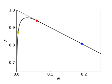
Figure 8: Near the bifurcation point, it takes longer than $T\sim-\varepsilon^{\star}\ln\varepsilon^{\star}$ to reach an $\mathcal{O}(\varepsilon^{\star})$–neighborhood of the slow manifold. In both panels, the thick black curve is the numerical solution to the dimensionless system (67) with $\varepsilon^{\star}=0.001$ and $\bar{c}(0)=\bar{w}(0)=0$. The thin, dash-dotted line is $\mathcal{S}_{1}$. The yellow square demarcates that position of the trajectory when $T=-\varepsilon^{\star}\ln\varepsilon^{\star}$. The red circle shows when $T=-\varepsilon_{\ddagger}\ln\varepsilon_{\ddagger}$ and the blue star at $T=-\sqrt{\varepsilon^{\star}}\ln\varepsilon^{\star}$. By inspection, it is clear that at $T=-\varepsilon^{\star}\ln\varepsilon^{\star}$, the trajectory is still not very close to $\mathcal{S}_{1}$. The right panel is a close-up of the left panel near the bifurcation point.

Now for the second scenario with $e_{0}<z_{0}$. Defining $\widehat{c}:=2c/E_{T}$, we recover the general dimensionless system:

$$\widehat{\varepsilon}\;\widehat{c}^{\prime} =(\sigma+\theta\bar{w}-\widehat{c})(\theta-\widehat{c}-\theta\bar{w})-\widehat{\varepsilon}\;\widehat{c},$$ (72a)

$$\bar{w}^{\prime} =\theta^{-1}\widehat{c},$$ (72b)

where $\widehat{\varepsilon}:=2k_{2}/k_{1}E_{T}$, $\sigma:=2e_{0}/E_{T}$ and $\theta:=2z_{0}/E_{T}$. If $\varepsilon_{\ddagger}\ll 1$ and $e_{0}<z_{0}$, the phase plane trajectory will rapidly approach $\mathcal{S}_{2}^{a}$, pass near the bifurcation point, and then follow $\mathcal{S}_{1}^{a}$ for the remainder of the reaction. Thus, the accuracy of the reduced problem is still limited to its accuracy in the neighborhood of the bifurcation point.

Proposition 4.

For any trajectory starting in $\Lambda^{*}$, the asymptotic validity of the reduced problem corresponding to (72) is limited by a term of $\mathcal{O}(\sqrt{\widehat{\varepsilon}}\;)$ in the neighborhood of the bifurcation point.

Proof: The distance, $d_{\mathcal{B}}$, from $\mathcal{S}_{1}\cap\mathcal{S}_{2}$ to $h^{-}(w_{T})$ is identically $\sqrt{K^{2}+2E_{T}K}-K$. Every trajectory starting in $\Lambda^{*}$ is bounded away from the bifurcation point by $d_{\mathcal{B}}$, which is bounded above by $\sqrt{2E_{T}K}$:

$$d_{\mathcal{B}}=\sqrt{K^{2}+2E_{T}K}-K\leq\sqrt{2E_{T}K}\sim\sqrt{K}.$$

Scaling this bound by $E_{T}/2$ (the maximal possible distance between $h^{-}(w_{T})$ and $\mathcal{S}_{1}\cap\mathcal{S}_{2}$) yields

$$\cfrac{2\sqrt{2E_{T}K}}{E_{T}}=2\sqrt{\cfrac{2K}{E_{T}}}\sim\mathcal{O}(\sqrt{\widehat{\varepsilon}}\;).$$ (73)

Our estimate (73) indicates that the scaling law of the dimensionless system (72) is proportional to the square root of the eigenvalue ratio is in agreement with established theoretical results. Trajectories of fast/slow systems in standard form (64) pass near dynamic transcritical bifurcation points at a distance that is of order $\sqrt{\varepsilon}$ (see [2] for a detailed overview of scaling laws near bifurcation points). The blow-up method [9, 31, 32] could possibly be utilized to rigorously explain the dynamics of the rQSSA (61) and the classical reduction (17) in neighborhoods containing $\mathcal{S}_{1}\cap\mathcal{S}_{2}$. However, such an analysis is beyond the scope of the paper, and will be the subject of a future work.

One practical challenge we face, both computationally and experimentally, is how to properly handle the switching undergone by the trajectory as it moves from one attracting submanifold to the other. To circumnavigate this difficulty, we utilize the classical reduction (17). From Proposition 1 we have

$$\varepsilon:=\bigg{(}\cfrac{k_{1}E_{T}}{k_{2}+k_{1}E_{T}}\bigg{)}\cdot\bigg{(}\cfrac{K}{\sqrt{K(K+2E_{T})}}\bigg{)},$$

which holds for all $e_{0}\leq z_{0}$. The upper bound

$$[\hat{c}-\hat{h}^{-}({w})]^{2} \leq[\hat{c}-\hat{h}^{-}({w})]^{2}(0)e^{\displaystyle-k_{1}\varphi t}+\varepsilon^{2},$$

$$=[\hat{c}-\hat{h}^{-}({w})]^{2}(0)e^{\displaystyle-k_{1}\varphi\cdot\cfrac{k_{2}}{k_{2}}\cdot t}+\varepsilon^{2},$$

$$=[\hat{c}-\hat{h}^{-}({w})]^{2}(0)e^{\displaystyle-T/\varepsilon}+\varepsilon^{2}$$

follows from Proposition 1, and with $k_{2}\ll k_{1}E_{T}$, $\varepsilon$ of Proposition 1 is approximately

$$\varepsilon\approx\cfrac{K}{\sqrt{K(K+2E_{T})}}\approx\sqrt{K/2E_{T}}\quad\text{for small}\;\;K.$$ (75)

We conclude from (75) that the classical reduction (17) is valid as long as $\sqrt{K/2E_{T}}\ll 1$.

5.3 A geometric interpretation of reversibility and the validity of the rQSSA

When reversibility is added to the binding step of the reaction mechanism (62) so that $k_{-1}\neq 0$ but $k_{2}=0$ in the singular limit, the layer problem consists of two disjoint critical manifolds, $c=h^{+}(w)$ and $c=h^{-}(w)$, and the set $\mathcal{C}^{\varepsilon}$ is no longer invariant. In this way, reversibility has an interpretation as a dynamic imperfection, since the bifurcation structure reported in figure 6 is broken (see figure 9).

Figure 9: Reversibility may be interpreted as an imperfection. Adding reversibility by setting $k_{-1}>0$ in the layer problem with $k_{2}=0$ yields two disjoint critical manifolds, $c=h^{-}(w)$ and $c=h^{+}(w)$. As indicated by the solid line, the critical manifold $c=h^{-}(w)$ is comprised of attracting fixed points. In contrast, the critical manifold $c=h^{+}(w)$ (dashed line) is comprised of repulsive stationary points. Note the bifurcation structure observed in Figure 6 is broken unless $k_{-1}=0$.

From Proposition 2, we see that the classical reduction’s accuracy improves with increasing $k_{-1}$. Moreover, the rQSSA (61) can still be successfully employed when $z_{0}\leq e_{0}$ provided $k_{-1}\ll k_{1}e_{0}$, and the validity of the rQSSA when $z_{0}=e_{0}$ is still regulated by a term that is proportional to $\sqrt{K_{M}/E_{T}}$. Again, the geometric interpretation is that $d_{\mathcal{B}}$ is

$$d_{\mathcal{B}}=\sqrt{K_{M}^{2}+2E_{T}K_{M}}-K_{M}$$ (76)

when $0<k_{-1}$, and thus the scaled distance is proportional to $\sqrt{K_{M}/E_{T}}$, while the total distance is ultimately proportional to $\sqrt{2E_{T}K_{M}}$. Since the distance from $h^{-}(w)$ to $\mathcal{S}_{1}$ decreases as $w\to z_{0}$ (i.e., because the stationary point $(c,w)=(0,z_{0})$ lies in the graphs of both $\mathcal{S}_{1}$ and $h^{-}(w)$), we expect the rQSSA (61) to improve as the ratio of $z_{0}$ to $e_{0}$ diminishes. Again, the blow-up method should be employed if one wishes to make more rigorous statements concerning the accuracy of the classical reduction and the rQSSA near the bifurcation point when $K_{M}\ll E_{T}.$

Remark 5.

To minimize the influence of the bifurcation point, an experiment should be prepared so that $z_{0}\ll e_{0}$ and $K_{M}\ll e_{0}$. Thus, the experimental qualifier, $K_{M}\ll E_{T},z_{0}\ll e_{0}$, is more restrictive than the mathematical qualifier, $K_{M}\ll E_{T},z_{0}\leq e_{0}$. Moreover, if in addition to $K_{M}\ll E_{T}$ it holds that $k_{2}\ll k_{-1}$, then the classical reduction (17) will yield the most accurate result; see Proposition 1.

6 Discussion

In this paper, we have found that the mass action equations of the IAZA reaction mechanism admit three possible QSS reductions: the standard QSSA (35), the reverse QSSA (61), and “total” QSSA (38). Furthermore, we have systematically derived the qualifiers (timescale ratios) that warrant the validity of a particular reduction (see, Table 1).

Parameter(s)	Qualifier	Approximation	Critical Set
$k_{1}$	$\varepsilon_{1}:=k_{1}E_{T}/(k_{-1}+k_{2})\leq tol.$	sQSSA (35)	$c_{1}=0$
$k_{2},k_{-1}$	$\widetilde{\varepsilon}\;\;:=\sqrt{(k_{-1}+k_{2})/k_{1}E_{T}}\leq tol.,\;\;\&\;\;z_{0}\leq e_{0}$	rQSSA (61)	$\mathcal{S}_{0}:=\mathcal{S}_{1}\cup\mathcal{S}_{2}$
$k_{2}$	$\varepsilon_{2}:=k_{2}/k_{-1}\leq tol.$	tQSSA (38)	$h^{-}(w;K_{S})$

Table 1: The parameters, qualifiers, and critical sets for the standard, reverse, and total QSSAs. The first column lists the dimensional parameters (rate constants) that, as a consequence of Fenichel theory, ensure the accuracy of the corresponding QSS reduction (third column) as they approach zero with all other parameters bounded away from zero. Of course, traditional Fenichel reduction does not apply to $\mathcal{S}_{0}$, but one can compute reductions that are valid along compact submanifolds of $\mathcal{S}_{0}$. The second column provides a metric (or stopping condition along the search direction defined by the parameter in the first column) that indicates how small one must make the parameter in the first column before the associated reduction (third column) is sufficiently accurate. The tolerance “$tol.$” in the second column can be used to define was is meant by sufficiently accurate. Mathematically, it is desirable that $tol.\ll 1$. However, there is limited resolution in laboratory measurements and, for experiments, a $tol.$ of $0.01$ is usually sufficient for an accurate QSS reduction [42]. The fourth column lists the critical set recovered in the singular limit that emerges when the parameter(s) in the first column is identically zero (with all other parameters bounded away from zero).

On the mathematical side, we have demonstrated that finding “$\varepsilon$,” can be a difficult task, as even planar systems can exhibit complicated phenomena, such as dynamic bifurcations where the classical results of GSPT are inapplicable. Additionally, the mathematical mechanism that warrants a QSS reduction may depend on the path one takes in parameter space. Here we have shown that the sQSSA is justifiable either from Fenichel reduction (as $k_{1}\to 0^{+}$), or from center manifold reduction (as $E_{T}\to 0^{+}$), and the mathematical justification depends on which parameter vanishes in the limit.

Our analysis of the IAZA reaction also alludes to a rather interesting research topic, which is the possible extension of TFPV theory to include dynamic bifurcation points. For example, it is understood that, due to the loss of normal hyperbolicity, asymptotic scaling laws change near bifurcation points [2]. The results of our analysis are consistent with the established scaling law near a transcritical bifurcation, as we demonstrated that the accuracy of the rQSSA when $z_{0}=e_{0}$ is proportional to $\sqrt{k_{2}}$ in the absence of reversibility. This suggests that if we define “$\varepsilon$” to be synonymous with $k_{2}$ via the mapping $k_{2}\mapsto\varepsilon k_{2}^{*}$, then the accuracy of the rQSSA for the irreversible mechanism should scale as $\sqrt{\varepsilon k_{2}^{*}}$ near $\mathcal{S}_{1}\cap\mathcal{S}_{2}$. While further investigation of this topic may appear moot or biochemically irrelevant with respect to experimental assay design, it should be noted that many in vivo reactions occur under conditions requiring stochastic fluctuations in the model equations. In such cases, it is necessary to resort to a Langevin equation or to the chemical master equation. Furthermore, QSS reductions of stochastic models are often adopted from the non-elementary rate equations generated from the deterministic QSS reduction and, interestingly, are frequently accurate under the same conditions that validate the deterministic QSS reduction [37, 27, 34]. QSS reductions of stochastic models are extremely useful in computational biology and computational medicine, as it is generally less expensive to simulate the reduced model [52]. Consequently, knowledge of both singular perturbation parameters, as well as scaling laws near bifurcation points, may help elucidate the validity of QSS approximations to stochastic models.

From the experimental perspective, we note that timescale separation is generally induced in laboratory experiments by preparing the reaction so that the ratio of initial enzyme concentration to reactant concentration is small (i.e., with $e_{0}\ll z_{0}$); see [14, 15, 59]. However, the condition $e_{0}\ll z_{0}$ does not ensure that the spectral gap of the Jacobian is wide enough to validate (16) or (17). This result differs from non-autocatalytic Michaelis Menten-type reactions, where a disparity in initial enzyme and substrate concentration is some times enough to ensure the validity of the standard QSS reduction [25, 45]. We also note that the IAZA reaction mechanism analyzed in the work was comparatively simple, and more complicated mechanisms have been proposed [14]. Moreover, most reactions can be controlled with inhibitors or activators. In the the presence of these modifiers, the determination of singular perturbation parameters for the reaction mechanism is much more difficult. This is because experimentally practical QSS reductions of three- and four-dimensional systems will generally result from projecting onto a one-dimensional slow manifold. Thus, while it may be that only one eigenvalue vanishes in the singular limit, the accuracy of the QSS reduction can require more than one dimensionless singular perturbation parameter to be small since there can be multiple fast timescales in higher dimensional systems; see [11] as an example. Understanding the qualifiers that ensure the accuracy of QSS reductions in higher-dimensional systems is critical if we are to make progress in metabolic engineering and drug development. And, as we have illustrated here, there is room for mathematics.

Appendix

6.1 Fenichel reduction in the small $k_{2}$ limit

In this appendix, we provide the full calculation for (36). To start, we define $k_{2}\mapsto\varepsilon k_{2}^{\star}$, and express the mass-action equations in perturbation form:

$$\begin{bmatrix}\dot{z}\\ \dot{c}\end{bmatrix}=\begin{bmatrix}-1\\ \;\;\;1\end{bmatrix}\bigg{(}k_{1}(E_{T}-z)z+(k_{-1}+2k_{1}z)c\bigg{)}+\varepsilon\begin{bmatrix}0\\ k_{2}^{\star}c\end{bmatrix}.$$

By inspection, we have

$$N(z,c):=\begin{bmatrix}-1\\ \;\;\;1\end{bmatrix},\quad f(z,c):=k_{1}(E_{T}-z)z+(k_{-1}+2k_{1}z)c,\quad\text{and}\quad G(z,c):=\begin{bmatrix}0\\ k_{2}^{\star}c\end{bmatrix}.$$

The derivative, $Df$ is the row vector

$$Df:=[\partial_{z}f\;\;\partial_{c}f],$$

where “$\partial_{x}$” denotes $\partial/\partial x$. Next, the term $NDf$ is an inner product and hence scalar-valued:

$$DfN:=\langle Df,N\rangle=-\cfrac{\partial}{\partial z}f(z,c)+\cfrac{\partial}{\partial c}f(z,c).$$

The projection operator, $\Pi^{M}$, is thus

$$\Pi^{M} =\mathbb{I}^{2\times 2}-N(DfN)^{-1}Df,$$

$$=\mathbb{I}^{2\times 2}-((DfN)^{-1})NDf,$$

and the QSS reduction (36) is

$$\dot{x}=\Pi^{M}G(z,c),\quad\text{evaluated at}\quad c=\cfrac{(E_{T}-z)z}{(2z+K_{S})},$$

with $x$ denoting $[z\;c]^{T}.$

6.2 Center manifold reduction in the small $E_{T}$ limit

Here we demonstrate that the QSS reduction, (35), is justified via center manifold reduction as $E_{T}\to 0^{+}$. First, we write the extended system

$$\begin{bmatrix}\dot{E}_{T}\\ \dot{z}\\ \dot{c}\end{bmatrix}=\begin{bmatrix}0&0&0\\ 0&0&k_{-1}\\ 0&0&-(k_{-1}+k_{2})\end{bmatrix}\begin{bmatrix}E_{T}\\ z\\ c\end{bmatrix}+\begin{bmatrix}\;\;\;0\\ \;\;\;1\\ -1\end{bmatrix}(2k_{1}zc-k_{1}(E_{T}-z)z),$$

which close enough to standard form. At lowest order, the local center manifold has the representation

$$c=h(z,E_{T})=\alpha z^{2}+\beta E_{T}z+\gamma E_{T}^{2}+\mathcal{O}(z^{3},E_{T}z^{2},E_{T}^{2}z,E_{T}^{3}).$$

To determine the coefficients $\alpha,\beta$ and $\gamma$, we substitute $h(z,E_{T})$ into the invariance equation,

$$D_{z}h(z,E_{T})\dot{z}(z,h(z,E_{T}))+D_{E_{T}}h(z,E_{T})\dot{E}_{T}=\dot{c}(z,h(z,E)),$$

and equate identical polynomial orders to zero. This yields $\alpha=-K_{M}^{-1},\beta=K_{M}^{-1}$ and $\gamma=0.$ Thus, $W_{\text{loc.}}^{c}(0)$ is given by

$$c\sim h(z,E_{T})=\cfrac{k_{1}(E_{T}-z)z}{k_{-1}+k_{2}},$$

and the dynamics of $z$ near the origin (and for small $E_{T}$) is given by

$$\dot{z}=-\cfrac{k_{2}}{K_{M}}(E_{T}-z)z+\mathcal{O}(z^{3},E_{T}z^{2}).$$

Consequently, we not only recover (35) in the small $E_{T}$ limit, we see that the vector field undergoes a transcritical bifurcation as $E_{T}$ moves from positive to negative.

References

- Al-Janabi et al. [1972] J. Al-Janabi, J. A. Hartsuck, and J. Tang. Kinetics and mechanism of pepsinogen activation. J. Biol. Chem., 247:4628–4632, 1972.
- Berglund and Gentz [2006] N. Berglund and B. Gentz. Noise-induced phenomena in slow-fast dynamical systems. Springer-Verlag London, Ltd., London, 2006.
- Bersani et al. [2015] A. M. Bersani, E. Bersani, G. Dell’Acqua, and M. G. Pedersen. New trends and perspectives in nonlinear intracellular dynamics: one century from michaelis–menten paper. Continuum Mech. Therm., 27:659–684, 2015.
- Bertram and Rubin [2017] R. Bertram and J. E. Rubin. Multi-timescale systems and fast-slow analysis. Math. Biosci., 287:105–121, 2017. 50th Anniversary Issue.
- Borghans et al. [1996] J. A. M. Borghans, R. J. De Boer, and L. A. Segel. Extending the quasi-steady state approximation by changing variables. Bull. Math. Biol., 58:43–63, 1996.
- Carr [1981] J. Carr. Applications of Centre Manifold Theory. New York: Springer-Verlag, 1981.
- Choi et al. [2017] B. Choi, G. A. Rempala, and J. K. Kim. Beyond the Michaelis–Menten equation: Accurate and efficient estimation of enzyme kinetic parameters. Sci. Rep., 7:17018, 2017.
- Desroches et al. [2012] M. Desroches, J. Guckenheimer, B. Krauskopf, C. Kuehn, H. M. Osinga, and M. Wechselberger. Mixed-mode oscillations with multiple time scales. SIAM Rev., 54(2):211–288, 2012. ISSN 0036-1445.
- Dumortier [1993] F. Dumortier. Techniques in the Theory of Local Bifurcations: Blow-Up, Normal Forms, Nilpotent Bifurcations, Singular Perturbations, pages 19–73. Springer Netherlands, 1993.
- Eilertsen and Schnell [2020] J. Eilertsen and S. Schnell. The quasi-steady-state approximations revisited: Timescales, small parameters, singularities, and normal forms in enzyme kinetics. Math. Biosci, 325:108339, 2020.
- Eilertsen et al. [2019] J. Eilertsen, W. Stroberg, and S. Schnell. Characteristic, completion or matching timescales? An analysis of temporary boundaries in enzyme kinetics. J. Theor. Biol., 481:28–43, 2019.
- Eilertsen et al. [2021] J. Eilertsen, M. Roussel, S. Schnell, and S. Walcher. On the quasi-steady-state approximation in an open Michaelis–Menten reaction mechanism. AIMS Math, 6, 2021.
- Fenichel [1979] N. Fenichel. Geometric singular perturbation theory for ordinary differential equations. J. Differ. Equations, 31:53–98, 1979.
- Fuentes et al. [2005] M. E. Fuentes, R. Varón, M. García-Moreno, and E. Valero. Kinetics of intra-and intermolecular zymogen activation with formation of an enzyme–zymogen complex. FEBS J., 272:85–96, 2005.
- García-Moreno et al. [1991] M. García-Moreno, B. H. Havsteen, R. Varón, and H. Rix-Matzen. Evaluation of the kinetic parameters of the activation of trypsinogen by trypsin. Biochim. Biophys. Acta, 1080:143–147, 1991.
- Goeke [2013] A. Goeke. Reduktion und asymptotische reduktion von reaktionsgleichungen. Doctoral Dissertation, RWTH Aachen, 2013.
- Goeke and Walcher [2014] A. Goeke and S. Walcher. A constructive approach to quasi-steady state reductions. J. Math. Chem., 52:2596–2626, 2014.
- Goeke et al. [2012] A. Goeke, C. Schilli, S. Walcher, and E. Zerz. Computing quasi-steady state reductions. J. Math. Chem., 50:1495–1513, 2012.
- Goeke et al. [2015] A. Goeke, S. Walcher, and E. Zerz. Determining “small parameters” for quasi-steady state. J. Differential Equations, 259:1149–1180, 2015.
- Goeke et al. [2017] A. Goeke, S. Walcher, and E. Zerz. Classical quasi-steady state reduction – A mathematical characterization. Physica D, 345:11–26, 2017.
- Goluskin [2010] D. Goluskin. Who ate whom: population dynamics with age-structured predation. Proceedings: WHOI GFD 2010 program of study: Swimming and swirling in turbulence, 2010.
- Guckenheimer and Holmes [1983] J. Guckenheimer and P. Holmes. Nonlinear Oscillations, Dynamical Systems, and Bifurcations of Vector Fields. New York: Springer-Verlag, 1983.
- Guckenheimer and Scheper [2011] J. Guckenheimer and C. Scheper. A geometric model for mixed-mode oscillations in a chemical system. SIAM J. Appl. Dyn. Sys., 10:92–128, 2011.
- Hanson and Schnell [2008] S. M. Hanson and S. Schnell. Reactant stationary approximation in enzyme kinetics. J. Phys. Chem. A, 112:8654–8658, 2008.
- Heineken et al. [1967] F. Heineken, H. Tsuchiya, and R. Aris. On the mathematical status of the pseudo-steady state hypothesis of biochemical kinetics. Math. Biosci., 1:95–113, 1967.
- Jardon-Kojakhmetov and Kuehn [2019] H. Jardon-Kojakhmetov and C. Kuehn. A survey on the blow-up method for fast-slow systems, 2019.
- Kang et al. [2019] H.-W. Kang, W. R. KhudaBukhsh, H. Koeppl, and G. A. Rempał a. Quasi-steady-state approximations derived from the stochastic model of enzyme kinetics. Bull. Math. Biol., 81:1303–1336, 2019.
- Kassell and Kay [1973] B. Kassell and J. Kay. Zymogens of proteolytic enzymes. Science, 180:1022–1027, 1973.
- Khan and James [1998] A. R. Khan and M. N. G. James. Molecular mechanisms for the conversion of zymogens to active proteolytic enzymes. Protein Sci., 7:815–836, 1998.
- Kimrey et al. [2020] J. Kimrey, T. Vo, and R. Bertram. Big ducks in the heart: Canard analysis can explain large early afterdepolarizations in cardiomyocytes. SIAM J. Appl. Dyn. Sys., 19(3):1701–1735, 2020.
- Krupa and Szmolyan [2001] M. Krupa and P. Szmolyan. Extending slow manifolds near transcritical and pitchfork singularities. Nonlinearity, 14:1473–1491, 2001.
- Kuehn [2015] C. Kuehn. Multiple Time Scale Dynamics, volume 191 of Applied Mathematical Sciences. Springer, 2015.
- Liu and Wang [2004] J. H. Liu and Z. X. Wang. Kinetic analysis of ligand-induced autocatalytic reactions. Biochem. J., 379(3):697–702, 2004.
- MacNamara et al. [2008] S. MacNamara, A. M. Bersani, K. Burrage, and R. B. Sidje. Stochastic chemical kinetics and the total quasi-steady-state assumption: Application to the stochastic simulation algorithm and chemical master equation. J. Chem. Phys., 129:095105, 2008.
- Noethen and Walcher [2009] L. Noethen and S. Walcher. Quasi-steady state and nearly invariant sets. SIAM J. Appl. Math, 70:1341–1363, 2009.
- Palsson and Lightfoot [1984] B. O. Palsson and E. N. Lightfoot. Mathematical modelling of dynamics and control in metabolic networks. I. On Michaelis-Menten kinetics. J. Theor. Biol., 111:273–302, 1984.
- Sanft et al. [2011] K. Sanft, D. T. Gillespie, and L. R. Petzold. The legitimacy of the stochastic Michaelis–Menten approximation. IET Syst. Biol., 5:58–69, 2011.
- Sanny et al. [1975] C. G. Sanny, J. A. Hartsuck, and J. Tang. Conversion of pepsinogen to pepsin. Further evidence for intramolecular and pepsin-catalyzed activation. J. Biol. Chem., 250:2635–2639, 1975.
- Schauer and Heinrich [1979] M. Schauer and R. Heinrich. Analysis of the quasi-steady-state approximation for an enzymatic one-substrate reaction. J. Theor. Biol., 79:425–442, 1979.
- Schnell and Maini [2000] S. Schnell and P. K. Maini. Enzyme kinetics at high enzyme concentration. Bull. Math. Biol., 62:483–499, 2000.
- Schnell and Maini [2002] S. Schnell and P. K. Maini. Enzyme kinetics far from the standard quasi-steady-state and equilibrium approximations. Math. Comput. Modelling, 35:137–144, 2002.
- Schnell and Maini [2003] S. Schnell and P. K. Maini. A century of enzyme kinetics. Reliability of the and estimates. Comments Theor. Biol., 8:169–187, 2003.
- Segel [1984] L. A. Segel. Modeling dynamic phenomena in molecular and cellular biology. Cambridge University Press, 1984.
- Segel [1988] L. A. Segel. On the validity of the steady state assumption of enzyme kinetics. Bull. Math. Biol., 50:579–593, 1988.
- Segel and Slemrod [1989] L. A. Segel and M. Slemrod. The Quasi-Steady-State Assumption: A case study in perturbation. SIAM Rev., 31:446–477, 1989.
- Shoffner and Schnell [2017] S. Shoffner and S. Schnell. Approaches for the estimation of timescales in nonlinear dynamical systems: Timescale separation in enzyme kinetics as a case study. Math. Biosci., 287:122–129, 2017.
- Stroberg and Schnell [2016] W. Stroberg and S. Schnell. On the estimation errors of and from time-course experiments using the Michaelis–-Menten equation. Biophys. Chem., 219:17–27, 2016.
- Tans et al. [1983] G. Tans, J. Rosing, and J. Griffin. Sulfatide-dependent autoactivation of human blood coagulation factor xii (hageman factor). J. Biol. Chem., 258:8215–22, 1983.
- Tans et al. [1987] G. Tans, J. Rosing, M. Berrettini, B. Lammie, and J. Griffin. Autoactivation of human plasma prekallikrein. J. Biol. Chem., 262:11308–14, 1987.
- Thrower et al. [2006] E. C. Thrower, A. P. E. Diaz de Villalvilla, T. R. Kolodecik, and F. S. Gorelick. Zymogen activation in a reconstituted pancreatic acinar cell system. Am. J. Physiol. Gastrointest. Liver Physiol., 290:G894–G902, 2006.
- Tikhonov [1952] A. Tikhonov. Systems of differential equations containing small parameters in their derivatives. Mat. Sb. (N.S.), 31:575–586, 1952.
- Turner et al. [2004] T. Turner, S. Schnell, and K. Burrage. Stochastic approaches for modelling in vivo reactions. Comput. Biol. Chem., 28:165–178, 2004.
- Tzafriri [2003] A. R. Tzafriri. Michaelis–menten kinetics at high enzyme concentrations. Bull. Math. Biol., 65:1111–1129, 2003.
- Varón et al. [2006a] R. Varón, M. García-Moreno, D. Valera-Ruiperez, F. Garcia-Molina, F. Garcia-Canovas, R. Ladron-de Guevara, J. Masia-Perez, and B. Havsteen. Kinetic analysis of a general model of activation of aspartic proteinase zymogens. J. Theor. Biol., 242:743–754, 2006a.
- Varón et al. [2006b] R. Varón, M. A. Minaya-Pacheco, F. García-Molina, E. Arribas, E. Arias, J. Masiá, and F. García-Sevilla. Competitive and uncompetitive inhibitors simultaneously acting on an autocatalytic zymogen activation reaction. J. Enzyme Inhib. Med. Chem., 21:635–645, 2006b.
- Vo et al. [2013] T. Vo, R. Bertram, and M. Wechselberger. Multiple geometric viewpoints of mixed mode dynamics associated with pseudo-plateau bursting. SIAM J. Appl. Dyn. Sys., 12(2):789–830, 2013.
- Wang et al. [2004] W.-N. Wang, X.-M. Pan, and Z.-X. Wang. Kinetic analysis of zymogen autoactivation in the presence of a reversible inhibitor. Eur. J. Biochem., 271:4638–4645, 2004.
- Wechselberger [2020] M. Wechselberger. Geometric Singular Perturbation Theory Beyond the Standard Forms. Springer, 2020.
- Wu et al. [2001] J.-W. Wu, Y. Wu, and Z.-X. Wang. Kinetic analysis of a simplified scheme of autocatalytic zymogen activation. Eur. J. Biochem., 268:1547–1553, 2001.