Optimizing timetable and network reopen plans for public transportation networks during a COVID19-like pandemic

Abstract

The recovery of the public transportation system is critical for both social re-engagement and economic rebooting after the shutdown during pandemic like COVID-19. In this study, we focus on the integrated optimization of service line reopening plan and timetable design. We model the transit system as a space-time network. In this network, the number of passengers on each vehicle at the same time can be represented by arc flow. We then apply a simplified spatial compartmental model of epidemic (SCME) to each vehicle and platform to model the spread of pandemic in the system as our objective, and calculate the optimal open plan and timetable. We demonstrate that this optimization problem can be decomposed into a simple integer programming and a linear multi-commodity network flow problem using Lagrangian relaxation techniques. Finally, we test the proposed model using real-world data from the Bay Area Rapid Transit (BART) and give some useful suggestions to system managers.

[table]capposition=top

1 Introduction

In response to the COVID-19 outbreak, the Center of Disease Control and Prevention (CDC) has promulgated guidance, including the practice of social distancing. The state of California also made intensive efforts and became the first state to issue a mandatory shelter-in-place order, which has largely mitigated the spread of the disease. Consequently, both the demand and supply for public transport decreased drastically from March to September.

As the situation evolves, regular activities will resume in the foreseeable future. Public transit, which is an integral part of personal lives, will become the first to face the sheer volume of crowds. Great concerns along with transmission relapse may be raised again when quantifying a crowded transportation system’s specific risk. It is worth noting that although many efforts have been made to model the spread of the disease and the public transportation network design problem has been thoroughly studied in the transportation literature, no clear guidance is available to public transit agencies during the recovery phase. In contrast, the infection risk of a pandemic like COVID-19 is not considered in the existing network planning and scheduling methods. Furthermore, safety measures such as social distancing and vehicle disinfection change the public transportation system’s working procedure. These factors need to be considered when drafting the recovery plan.

Therefore, a reopening design method considering the risk of new infection is needed for public transportation and becomes more urgent in the coming months. Taking the active social distancing order and the risk of new infection into consideration, we address the following problems simultaneously: (1) Network reopening design: how to re-gauge the network and determine which lines and stations to open in the given region. We need to decide if we can open each line or station at the beginning of the day; (2) Timetable design: how to design a timetable to satisfy all demands and control the risk of new cases. We need to decide when we should dispatch one train on line $l$, assuming a fixed travel time. We say one train on line $l$ is dispatched at time $t$ if one train of line $l$ leaves its first stop and start a new run. We call one train operation a ‘dispatch’ and we use term ‘run’ and ‘dispatch’ interchangeably in this paper.

1.1 Pandemic and travel

The COVID-19 pandemic has dramatically impacted the global economy in 2020, with 167K deaths and $>5$M confirmed cases in the US alone by September 2020 [28].

The transmission mechanism of COVID-19 and other similar epidemics have been studied by public health researchers from January to August, and new results are being consistently obtained. It is already known that COVID-19 can be transmitted directly from person to person through respiratory droplets [14], and it is likely that “a person can get COVID-19 by touching a surface or object that has the virus on it” [15]. The disease is highly contagious, with a reproduction rate of $R_{0}$ estimated to be $2.7$ to $5.7$ in Wuhan, China [42] in September 2019 and 6.4 in New York State [27] in March 2020.

To model the transmission of COVID-19 or other pandemic in a public transit network, the spatial nature of the pandemic’s spread should be captured explicitly. There are plenty of studies on modeling the spread of pandemics in the mathematical epidemiology literature (see books such as [3], [12], and [37]). Generally, the pandemic spread can be modeled using a network where each node represents one location (a city, province, or block). Inside each node, the pandemic spread according to differential or difference equations, similar to the Susceptible, Infectious, or Recovered (SIR) model.

During the COVID-19 pandemic, researchers have further developed these models to evaluate COVID-19 travel policies. Chinazzi [17] studied the impact of travel restrictions in China. They used the global epidemic and mobility model (GLEAM) and model regions as nodes in a metapopulation network based on air transportation data. Jia et al.[29] developed a spatiotemporal ‘risk source’ model to assess the risk of COVID-19 community transmission using the actual movement data of cell phone users. They modeled the infection based on a multiplicative exponential model and predicted the number of new infections in cities or provinces outside Wuhan. Li et al.[33] simulated the spatiotemporal dynamics of infection and inferred important parameters using an iterative filtering-ensemble adjustment Kalman filter framework. They concluded that the transmission rate $\beta$ in spatial compartmental models is $1.12$ ($95\%$ CI $[1.06,1.19]$). This parameter captures the rate at which an infected agent infects others and plays an important role in our model.

Based on these models, operations management and economics researchers have studied the optimal lockdown or reopen decision making aspects during the pandemic. Birge et al.[11] proposed a spatial compartmental model of epidemics (SCME) that was an extension of the works of [3][12][37].They optimized the neighborhood travel ban/reopen plan policy in New York City. [31] proposed a decision-making model implemented at Yale University. Alvarez et al.[4] attempted to find the optimal lockdown policy to minimize the loss. Other researchers such as [1][22][23] used heterogeneous Susceptible-Infectious-Removed (SIR) or Susceptible-Exposed-Infectious-Removed (SEIR) models to make critical decisions on the lockdown period or medical supply distribution during the pandemic.

1.2 Pandemic and public transit

The COVID-19 pandemic has heavily impacted public transit systems in the US. For example, in the bay area, Bay Area Rapid Transit (BART) implements social distancing procedures, and masks are mandatory. They use hospital-grade disinfectants to clean the carts multiple times a day [7]. AC transit, who provide bus services to the east San Francisco Bay Area, have modified the timetable and canceled some line services [2]. Ridership in New York dropped by 92% in mid-April, and night services are no longer available [20]. Similar measures have been implemented by different transit agencies across the US [6][16].

To date (May 2021), there is no confirmed evidence of COVID-19 transmission via public systems as long as proper precautions and necessary safety measures are in place [30][41][43]. However, the public transit system may play some role in the spread of the disease [15] which is supported by the early cases in Hunan and Zhejiang, China [36][44], and the risks must be considered when a reopening plan is drafted for the transit systems. Transportation researchers are now trying to model the pandemic within public transportation systems [38] [32] [35]. Mo et al.[38] modeled the pandemic using an public transportation encounter network (PTN) and an epidemic transmission model.

1.3 Space-time transit network design problem

The aim of this study is to integrate public transit network reopen plan and timetable optimization. The transit network reopen is a network design problem aiming to determine the network layout, frequencies, timetables, and ticket prices. Transportation network design has been studied for decades. The reader can refer to survey papers such as [19][24][26] and some of the latest papers on this topic [5][13][18].

The integrated transit network and timetable design problem can be formulated as a two-level network design problem. The upper level involves the design problem with integer design variables, while the lower-level problem is the traffic assignment problem with path or link flow variables. The formulation of the lower-level problem depends on the assumption of the user routing choice. One typical assumption is user equilibrium (UE), that is, Wardrop’s first principle. UE assumes that a Nash equilibrium will be achieved among all users once the network design is given. For example, in [21], the UE condition was formulated as variational inequalities. Their algorithm can determine a near-optimal network layout and frequency design of a transit system. However, the arc capacity constraints were not explicitly stated in their model. Verbas and Mahmassani[47] assumed an elasticity of travel demand and optimized the frequency allocation.

Another common assumption made when solving the integrated network and timetable design problem is the system optimal (SO), that is, Wardrop’s second principle. It assumes that the manager can control the route choice of all users. When the SO is assumed, the two-level problem becomes a one-level optimization problem because the decision-maker determines all the decision variables, so the problem is usually easier to solve than UE. For example, in Niu’s papers [39] and [40], the authors only considered a railway corridor, and there were no transfers so that the SO could be defined analytically. Although they only considered one simple corridor, they used a space-time network with a time dimension, so their nonlinear network UE was still complicated to solve. Szeto and Jiang [45] considered a capacitated static transit network with transfers, and as the lower-level problem became linear, the SO could be solved efficiently.

Besides the SO and UE, users can be assumed to be boundedly rational, where the users will comply with the system assigned path as long as the path does not cost much more than the current shortest path. Liu and Zhou [34] used this assumption and built an agent-based space-time network. Their model captured many subtle behaviors of the passengers, such as transfer and waiting time on platforms.

1.4 Potential contributions and structure of this paper

The contributions of this work can be summarized as follows: (1) Providing references to transportation managers. We will answer several important questions: How can the public transportation system look ahead to meet the challenge of demand during the pandemic? How can the existing transit network be reopened? How can we design an optimal schedule? (2) Novel formulation of a pandemic in public transit systems. We use a space-time dynamic transit network to capture complicated behaviors such as transfers and waiting at platforms, and we capture the risk of pandemic transmission using a simplified spatial compartmental model of epidemics (SCME) [11] (3) Efficient algorithms for similar problems. Although the full formulation is difficult to solve because of a huge number of variables and constraints, we show that with Lagrangian relaxation, the problem can be decomposed into two subproblems. One subproblem involves a multi-commodity network flow problem, while an off-the-shelf solver such as Gurobi [25] can be used to solve the other subproblem.

The remainder of this paper is organized as follows. In section 2, we present the assumptions of our model, and detail the formulation of our dynamic transit network considering the pandemic risk and social-distancing measures. A simple example is used to illustrate the major features of the dynamic network. In Section 3, we formulate the dynamic network design problem with pandemic risk as our objective function and social-distancing constraints, and the Lagrangian relaxation procedure used to solve this problem is presented in section 4. In section 5, we validate our model using real-world data from the BART system in the San Francisco Bay Area and provide an optimal timetable design. In section 6, the conclusions and potential future research questions are presented.

2 Space-time transit network with epidemic/pandemic

Consider a city planing to reopen public train/bus network under a pandemic similar to COVID-19. We will call this pandemic ‘the pandemic’ in the following sections. We will build a space-time passenger flow network in section 2.1, and we will integrate epidemic/pandemic model with this network in section 2.2.

2.1 Space-time transit network model

2.1.1 Physical network

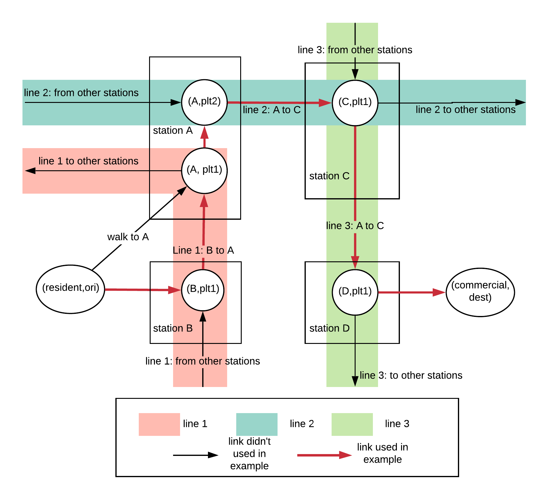
Figure 1: Physical network

Consider a city with three types of locations: $\mathcal{S}\cup\mathcal{O}\cup\mathcal{D}$, where $\mathcal{S}$ is the set of stations, $\mathcal{O}$ is the set of origin areas, and $\mathcal{D}$ is the set of destination areas. In each station $s$, there could be one or many platforms $plt_{j}\in PLT(s)$, where $PLT(s)$ is the set of platforms in station $s$. In many real-world systems, multiple lines can share one platform while it is also common that one station has many platforms for different lines.

Let the set of all candidate bus/train lines be $\mathcal{L}=\{0,1,...,|\mathcal{L}|\}$, and the set of lines passing station $s\in\mathcal{S}$ using platform $plt_{j}$ be $\mathcal{L}(s,plt_{j})$. One line consists several arcs connecting platforms from one station to another.

There are three types of nodes in our network: origin, destination, and platforms. We use tuple $(i,k)$ to index nodes in $\mathcal{N}^{0}$, where $i\in\mathcal{S}\cup\mathcal{O}\cup\mathcal{D}$ represent the physical location of the node, and $k\in\{ori,dest\}\cup\{plt_{j}\in PLT(s)\}$ represent the types of the nodes. $k$ can be any one of the following:

• $ori$: origin

• $dest$: destination

• $plt_{j}$: platform $plt_{j}$ for in station $s$

For example, node $(A,plt_{1})$ in figure 1 is the platform 1 at station A, and node $(resident,ori)$ is the origin node at the ‘resident’ area.

Using this index rule, the set of nodes $\mathcal{N}^{0}$ is the union of set of origin nodes $\{(o,ori):o\in\mathcal{O}\}$, the set of destinations $\{(d,dest):d\in\mathcal{D}\}$, and the set of all platforms $\{(s,plt_{j}):s\in\mathcal{S},plt_{j}\in PLT(s)\}$

$$\mathcal{N}^{0}:= \{(o,ori):o\in\mathcal{O}\}\cup\{(d,dest):d\in\mathcal{D}\}\cup\{(s,plt_{j}):s\in\mathcal{S},plt_{j}\in PLT(s)\}$$

There are also several types of arcs, as is illustrated in figure 1, including walking arcs between origins/destinations and stations, in-vehicle travel arcs between platforms of the same line at two different stations, and transfer arcs from one platform to another at the same station. Note that there are two types of transfers: transfers using the same platform, and transfers using different platforms. We use set $\mathcal{A}^{0}$ to represent all arcs described above. The physical network is defined as

$$(\mathcal{N}^{0},\mathcal{A}^{0})$$

We can illustrate the network using a simple example in figure 1. Given sets of physical locations $\mathcal{O}=\{resident,...\}$, $\mathcal{D}=\{commercial,...\}$, $\mathcal{S}=\{A,B,C,D...\}$ and set of lines $\mathcal{L}=\{1,2,3...\}$, where line 1 (red) connects station B to A, line 2 (blue) connects station A to C, and line 3 (green) connects station C to D. Consider one passenger travel from the ‘resident’ area to the ‘commercial’ area. He/she can take line 1 from station B to station A, transfers to line 2 at station A, transfers to line 3 at station C, takes line 3 from station A to station C, and walk to the commercial area. His/her trajectory is plotted in figure 1 using red arcs. Note that in station A, there are two platforms so that transfer passengers need to change their platforms, while in station C, all lines use the same platform.

2.1.2 Space-time network

During a pandemic like COVID-19, the capacity of each vehicle is strictly limited according to the social distancing rules. Therefore, we need to know the exact number of passengers on each vehicle and impose a strict social distancing capacity constraint, instead of just calculating the average number of passengers and compare it with the capacity. In addition, we need to track all passengers who stayed at the same vehicle or waited at the same platform with patients, since infection may happens on platforms or vehicles. Besides, we want to know the exact waiting time to optimize the timetable so that passengers can transfer between different lines smoothly.

We cannot answer these questions using the physical network in section 2.1.1, which can only give network flows averaged over time. We need to add an time dimension to the network and model the city as a space-time network similar to the models in [18][39][40]. The idea is to make many copies of the nodes physical network and connect them using different types of arcs representing in-vehicle travelling, waiting on the platforms, walking, and early/late departure/arrival.

Recall that the set of locations is $\mathcal{O}\cup\mathcal{S}\cup\mathcal{D}$, the set of lines is $\mathcal{L}$, and for each station $s\in\mathcal{S}$, $\mathcal{L}(s,plt_{j})\subset\mathcal{L}$ is the set of lines coming through station $s$ using platform $plt_{j}$. Consider a discrete time horizon $\mathcal{T}:=\{1,2,3,...\}$, we make $|\mathcal{T}|$ copies of $\mathcal{N}^{0}$ in the physical network and add a time index to each node. In this network, each node can be represented by a tuple $(i,k,t)$, where $i\in\mathcal{O}\cup\mathcal{S}\cup\mathcal{D}$ is the physical location, $k\in\{ori,dest\}\cup\{plt_{j}\in PLT(s)\}$ is the type of the node (defined in 2.1.1), and $t\in\mathcal{T}$ is the time step. Mathematically, the set of nodes is defined as:

$$\mathcal{N}:=\bigcup_{t\in\mathcal{T}}\mathcal{N}^{t}$$

Where we make $|\mathcal{T}|$ copies of the node set in physical network:

$$\mathcal{N}^{t}:= \{(o,ori,t):o\in\mathcal{O}\}\cup\{(d,dest,t):d\in\mathcal{D}\}$$

$$\cup\{(s,plt_{j},t):s\in\mathcal{S},plt_{j}\in PLT(s)\}$$

In words, node set $\mathcal{N}^{t}$ at each time step $t$ is the union of the set of origin nodes, the set of destinations, and the set of all platforms. $\mathcal{N}$ is the union of all $|\mathcal{T}|$ of $\mathcal{N}^{t}$s.

Using the nodes defined, let the platform for line $l$ at station $s$ be $plt(l,s)$, we can construct the whole space-time network using the following 6 types of arcs:

$$\mathcal{A}:=\mathcal{A}_{transfer}\cup\mathcal{A}_{travel}\cup\mathcal{A}_{wait}\cup\mathcal{A}_{os}\cup\mathcal{A}_{sd}\cup\mathcal{A}_{dd}$$

Where sets are defined:

• $\mathcal{A}_{transfer}:=\{(s,plt(l_{1},s),t)\rightarrow(s,plt(l_{2},s),t),\forall s\in\mathcal{S},l_{1},l_{2}\in\mathcal{L}(s),t\in\mathcal{T}\}$ contains arcs between two platforms the same station, where $\mathcal{L}(s)$ is the set of lines travelling through station $s$. Note that we ignore the walking time inside the stations.

• $\mathcal{A}_{travel}:=\{(s_{1},plt(l,s_{1}),t)\rightarrow(s_{2},plt(l,s_{2}),t+\Delta t_{s_{1},s_{2},l})|s_{1},s_{2}\in\mathcal{S},l\in\mathcal{L}(s_{1})\cap\mathcal{L}(s_{2})$, $t\in\mathcal{T}$, $s_{1},s_{2}$ are two consecutive stations on line $l\}$ contains arcs between platforms of the same line at different stations. These are in-vehicle travel arcs, where $\Delta t_{s_{1},s_{2},l}$ is the train running time from $s_{1}$ to $s_{2}$ on line $l$, $plt(l,s)$ is the platform that line $l$ used at platform $s$.

• $\mathcal{A}_{wait}:=\{(s,plt(l,s),t)\rightarrow(s,plt(l,s),t+1)|s\in\mathcal{S},l\in\mathcal{L}(s,plt_{i})$, $t\in\mathcal{T}\}$ contains arcs between the same platform at different time period. These are platform waiting arcs where passengers can wait until the next available train/bus arrival, $plt(l,s)$ is the platform that line $l$ used at platform $s$.

• $\mathcal{A}_{sd}:=\{(s,plt_{j},t)\rightarrow(d,dest,t+\Delta t_{s,d})|s\in\mathcal{S},d\in\mathcal{D},t\in\mathcal{T},plt_{j}\in PLT(s)\}$ contains walking arcs from stations to destinations, where $\Delta t_{s,d}$ is walking time from $s$ to $d$.

• $\mathcal{A}_{os}:=\{(o,ori,t)\rightarrow(s,plt_{j},t+\Delta t_{o,s})|s\in\mathcal{S},o\in\mathcal{O},t\in\mathcal{T},plt_{j}\in PLT(s),\Delta_{min}<\Delta t_{o,s}<\Delta_{max}\}$ contains walking arcs from origins to stations, where $\Delta t_{o,s}$ is walking time from $o$ to $s$ plus early/late departure time difference. We allow passengers to leave earlier or later than their desired departure time, but the time difference is bounded: the time difference between desired departure time and the time that passenger enters one station must lies in $\Delta_{min},\Delta_{max}$. In our numerical examples, we set $\Delta_{min}=-30$ min and $\Delta_{max}=30$ min.

• $\mathcal{A}_{dd}:=\{(d,dest,t_{1})\rightarrow(d,dest,t_{2}),\forall t_{1},t_{2}\in\mathcal{T}\}$. These arcs connects all destination nodes of the same location together, so as long as the passenger arrive in their destination, they can complete their journey.

We define the set of time dependent OD pairs:

$$\mathcal{W}:=\{((o,ori,t),(d,dest,t))|o\in\mathcal{O},d\in\mathcal{D},t\in\mathcal{T}\}$$

and for each $w\in\mathcal{W}$, the demand is $d_{w}$.

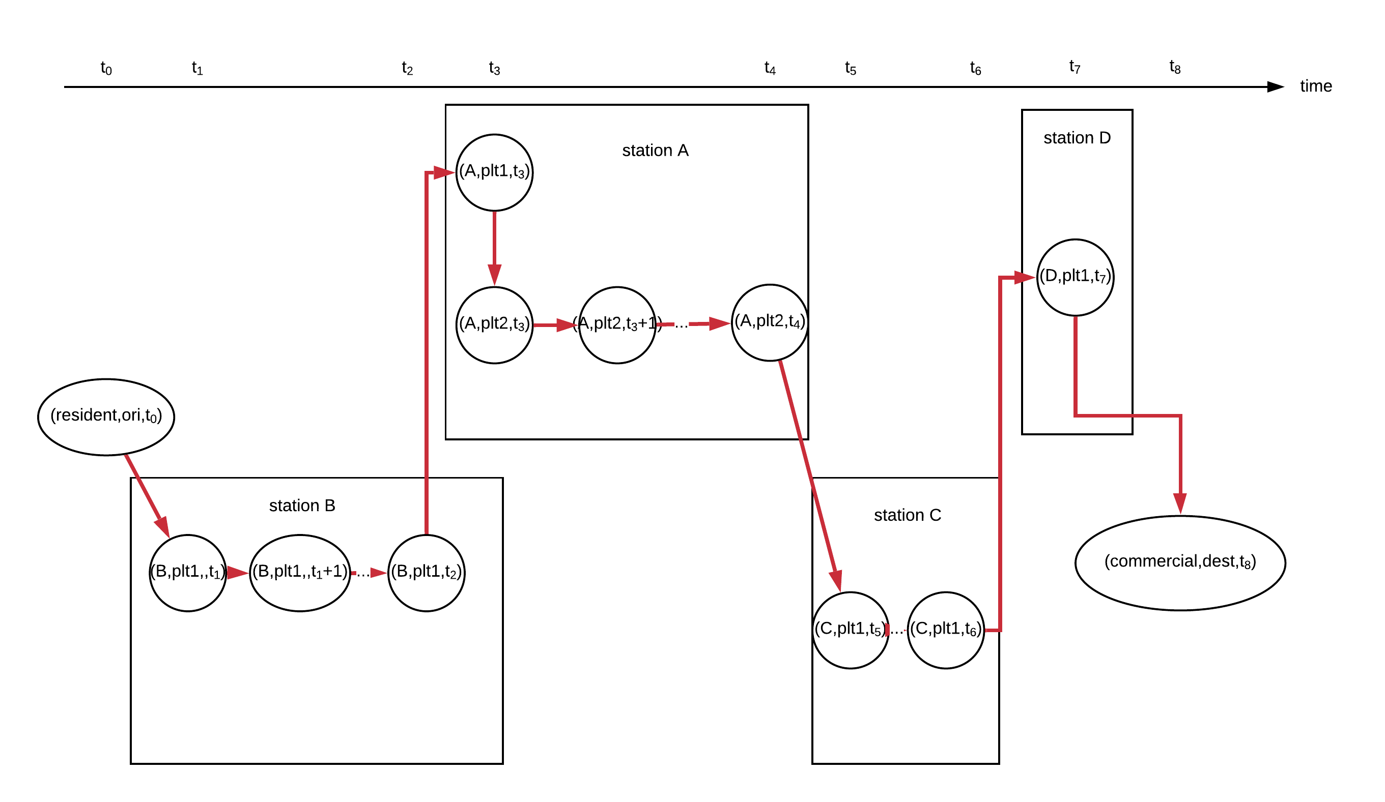
Figure 2: Trajectory on space-time network

Consider the previous example in figure 1, the passenger’s trajectory on the space-time graph is in figure 2. The whole process is:

1. Walking from resident to station B’s platform $plt_{1}$. This arc is in set $\mathcal{A}_{os}$.

   $$(resident,ori,t_{0})\rightarrow(B,plt_{1},t_{1})$$

2. Waiting at the platform until the next train from line 1 arrives at station B. These arcs are in set $\mathcal{A}_{wait}$

   $$(B,plt_{1},t_{1})\rightarrow(B,plt_{1},t_{1}+1)\rightarrow...\rightarrow(B,plt_{1},t_{2})$$

3. Riding a train/bus from B to A using line 1. $t_{3}-t_{2}$ is the in-vehicle travel time. This arc is from $\mathcal{A}_{travel}$

   $$(B,plt_{1},t_{2})\rightarrow(A,plt_{1},t_{3})$$

4. Making transfer from line 1 to line 2 at station A, assuming the transfer takes $t_{4}-t_{3}$. This arc is in set $\mathcal{A}_{transfer}$.

   $$(A,plt_{1},t_{3})\rightarrow(A,plt_{2},t_{3})$$

5. Waiting at station A. These arcs are in set $\mathcal{A}_{wait}$.

   $$(A,plt_{2},t_{3})\rightarrow(A,plt_{2},t_{3}+1)\rightarrow...\rightarrow(A,plt_{2},t_{4})$$

6. Riding line 2 to station C, assuming the travel time from station A to C on line 2 is $t_{5}-t_{4}$

   $$(A,plt_{2},t_{4})\rightarrow(C,plt_{1},t_{5})$$

7. Waiting for line 3 at the same platform, and travelling to station D

   $$(C,plt_{1},t_{5})\rightarrow(C,plt_{1},t_{6})\rightarrow(D,plt_{1},t_{7})$$

8. Walking to commercial area from station $C$, assuming it takes $t_{8}-t_{7}$ to walk from station C to ’commercial’ area.

   $$(D,plt_{1},t_{7})\rightarrow(commercial,dest,t_{8})$$

2.2 SCME model on the time-space network

According to pandemic models like SCME [11] models. We know that pandemic like COVID-19 transmission happens when susceptible passengers stay with patients in the same location for a certain period of time. In other words, a healthy person must spend some time with a patient together to get infected.

If we ignore the walking time inside stations (see assumption 4 in section 3.1), the pandemic transmission happens only when susceptible passengers stay with patients in the same vehicle or on the same platform for a period of time. Using the dynamics from SCME [11], we treat each origin node $o\in\mathcal{O}$ as the place where population lived, and each in-vehicle travel link and on-platform waiting link as place where transmission happens. We ignore the dead population since our time horizon is short. We consider people in three categories: healthy but not immune (susceptible), cured or vaccinated, and infected (exposed + clinical infected + subclinical infected). The daily new cases for population living in area $o\in\mathcal{O}$ is

$$\Delta IP_{o}=\beta\sum_{(i,j)\in\mathcal{A}_{travel}\cup\mathcal{A}_{wait}\cup\mathcal{A}_{transfer}}TT_{o,(i,j)}IR_{ij}$$ (1)

where $IP_{o}$ is the infected population in area $o$, $\Delta IP_{o}$ is the expected number of new cases, $TT_{o,(i,j)}$ is the total time that susceptible people from area $o$ spent on link $(i,j)$, and $IR_{ij}$ is the infection rate of all passengers on link $(i,j)$. $\beta$ is the transmission rate ($\approx 1.12$ for COVID-19 [33]). For example, if $5$ susceptible passengers from origin $o$ stay in the same train from $i$ to $j$ and the travel time is $6$ minutes, then $TT_{o,(i,j)}=5\times 6=30$ minutes. If there is one patients in a train from $i$ to $j$ with other 99 healthy (susceptible) passengers, then $IR_{ij}=0.01$.

Let the network flow of $w\in\mathcal{W}$ on link $(i,j)$ be $u_{ij}^{w}$, the travel time of link $(i,j)$ be $c_{ij}$, and the ratio of susceptible population be $q_{s}$ (healthy people who have never been infected and have not taken vaccine) we can calculate the total time that people from $o$ spent on link $(i,j)$:

$$TT_{o,(i,j)}=\sum_{w:\ origin\ is\ o}u_{ij}^{w}c_{ij}q_{s}$$ (2)

Let the probability that a person from OD pair $w$ is infected be $q_{w}$, we can calculate the infection rate on link $(i,j)$:

$$IR_{ij}=\frac{\sum_{w\in\mathcal{W}}u_{ij}^{w}q_{w}}{\sum_{w\in\mathcal{W}}u_{ij}^{w}}$$ (3)

Plug 2 and 3 into 1, we can estimate the new infections in our transit system among people from origin $o$,

$$\Delta IP_{o}=\beta q_{s}\sum_{(i,j)\in\mathcal{A}_{travel}\cup\mathcal{A}_{wait}\cup\mathcal{A}_{transfer}}\sum_{w_{o}:\ origin\ is\ o}u_{ij}^{w_{o}}c_{ij}\frac{\sum_{w\in\mathcal{W}}u_{ij}^{w}q_{w}}{\sum_{w\in\mathcal{W}}u_{ij}^{w}}$$ (4)

Therefore, we can simply sum all infections together to estimate the total number of new infections in our system:

$$\begin{split}\Delta IP&=\beta q_{s}\sum_{(i,j)\in\mathcal{A}_{travel}\cup\mathcal{A}_{wait}\cup\mathcal{A}_{transfer}}\sum_{w_{o}\in\mathcal{W}}u_{ij}^{w_{o}}c_{ij}\frac{\sum_{w\in\mathcal{W}}u_{ij}^{w}q_{w}}{\sum_{w\in\mathcal{W}}u_{ij}^{w}}\\ &=\beta q_{s}\sum_{(i,j)\in\mathcal{A}_{travel}\cup\mathcal{A}_{wait}\cup\mathcal{A}_{transfer}}c_{ij}\sum_{w\in\mathcal{W}}u_{ij}^{w}q_{w}\end{split}$$ (5)

3 Network and timetable design problem under the pandemic

3.1 Assumptions

We make these key assumptions:

1. Users are boundedly rational.

2. Buses/trains are capacitated.

3. The OD demand at each time step is deterministic, and the system will serve all the demand.

4. Walking time inside stations is ignored.

5. Bus/train travel time between two stations are fixed.

6. Buses/trains need to be cleaned and disinfected at the last station after one run.

7. The train dwell time is ignored, and passenger boarding takes no time.

8. Assumptions on the pandemic as in section 2.2.

In assumption 1, we assume users are boundedly rational, similar to model in [34], that the system manager can control the flow of passengers to some degree, but only when the users are deviated from the shortest path by limited amount of time. The manager can control the flo by changing the ticket price, enforcing capacity rules so that passengers are forced to change route when a cart reaches its capacity, or releasing real-time on-board crowd data so that passengers know the risk and they will avoid crowded areas for their own safety concerns.

When demand is small and capacity constraints are loose, our optimization problem 20 will give an all-pair shortest path solution, which is the only user equilibrium, because the objective function is linear. When demand is large, the optimization problem 19 gives one of the equilibrium: one user cannot improve his/her cost by changing route, because all better routes are congested. With the boundedly rational assumption, we know this equilibrium is similar to the actual equilibrium in real life, where people greedily look for the shortest path. Moreover, during the pandemic, some transit agencies got temporary power to manage passenger flow network by rejecting entrance to stations. In this case, agencies can manage the network flow and system optimal/boundedly rational can be achieved. For example, in mid-March, the government requires that every passenger submits application before using the bus system [46].

In assumption 2, we assume that bus/train is capacitated due to the social distancing order. Although in some public transportation system like SF BART, there is no supervisors in the stations and the limit-capacity social distancing rule seems not mandatory. However, BART provides real-time on-board crowd data to public [7] and people who are concerned may check these information and decide whether boarding the next train or not. According BART’s data, in most of the cases, the actual number of passengers are smaller than the requirement of social distancing capacity and the capacity constraints are valid.

In assumption 3, we assume that all time-dependent OD demand must be satisfied. Considering the fact that people who need public transportation system during a pandemic like COVID-19 usually don’t have access to other means of transportation like private cars, while carpool service suspends and taxis are expensive. In addition, during a pandemic like COVID-19, people are required to ‘go out only when necessary’ so travel demand are deemed ‘necessary’. Therefore, in our model, all demand must be satisfied, otherwise the problem is not feasible.

In assumption 4, we ignore the walking time inside the station so that we only need to consider the transmission on platforms and vehicles (see our SCME model in section 2.2). Noting that passengers spent most of their time waiting on platforms and staying in vehicles while using public transportation systems, and the time that passengers spend walking inside the stations (usually less than 1 min) can be ignored compared to waiting time and traveling time (can be $>10$ min), so this assumption is close to reality.

In assumption 5, we assume that the running time between two stations is constant. Because when train/bus follows the timetable, there is no congestion in most of the mass transit systems if no accident happens. The travel time from station to station can be deemed as fixed since there is little congestion for bus system during the pandemic, and the travel time is relatively stable in railway systems.

During the pandemic like COVID-19, we know trains/buses need to be disinfected after each run. We assume in assumption 6 that this happens only at the last station.

We also ignore the train/bus dwell time at stations as assumption 7, since vehicles in mass transit like BART spend most time travelling [9].

The last assumption is valid for public transportation systems: it is only possible that a healthy passenger to get the pandemic when an infected passenger stays within a certain distance.

3.2 Notations

We only list important notations used in our optimization model. You can find the definition of different sets of arcs and nodes in section 2.2.

Table 1: Notations

Sets
$\mathcal{O}$	set of origin nodes (physical)
$\mathcal{D}$	set of destination nodes (physical)
$\mathcal{S}$	set of station nodes (physical)
$\mathcal{S}_{0}$	set of the first/last station for each line, $\mathcal{S}_{0}\subset\mathcal{S}$
$\mathcal{L}$	set of bus/train lines
$\mathcal{T}$	set of time
$\mathcal{N}$	set of all nodes in space-time network
$\mathcal{A}$	set of all arcs in space-time network
$\mathcal{W}$	set of OD pairs
$\mathcal{L}^{in}(s)$	set of lines using $s$ as the last stop
$\mathcal{L}^{out}(s)$	set of lines using $s$ as the first stop
$\mathcal{P}_{w}$	set of all paths of OD pair $w$
$\mathcal{P}_{w}^{\prime}$	set of paths of OD pair $w$ satisfying boundedly rational condition
Continuous variables
$\pi_{lt}$, $\mu_{s}$	Lagrangian multipliers
$f_{w}^{p}$	flow on path $p$ in the path-flow formulation
$u_{ij}^{w}$	arc flow on $(i,j)$ of OD pair $w\in\mathcal{W}$
$v_{ij}$	arc flow on $(i,j)$
Integer variables
$x_{lt}$	binary, $=1$ if line $l$ is opened and one train is dispatched at time $t$
$y_{s}$	binary, $=1$ if station $s\in\mathcal{S}$ is opened
$z_{l}$	binary, $=1$ if line $l\in\mathcal{L}$ is opened
$M_{s}$	number of trains available at station $s\in\mathcal{S}_{0}$ at the beginning of the day
Parameters
$\alpha_{ij}^{p}$	$=1$ if path $p$ will use arc $(i,j)$
$\beta$	transmission rate
$B$	budget
$c_{i,j}$	link travel time of $(i,j)$
$c_{i,j}^{w}$	link cost with multipliers of $(i,j)$ for users from $w$
$C_{p}$	cost of path $w$ with multipliers
$c_{l,open}$	cost of opening a new line $l$
$c_{l,close}$	cost of closing an existing line $l$
$c_{s,open}$	cost of opening a new station $s$
$c_{s,close}$	cost of closing an existing station $s$
$c_{l,t}$	cost of dispatching one train at time $t$ of line $l$
$d_{w}$	demand of OD pair $w\in\mathcal{W}$
$M_{0}$	total number of available trains
$N_{ij}$	capacity of link $(i,j)$ under social distancing rules
$q_{w}$	infection rate of OD pair $w\in\mathcal{W}$
$q_{s}$	ratio of suseptiable people
$z_{l}^{0}$	$=1$ if line $l$ is already opened
$SP(w)$	one of the shortest paths for OD pair $w$, $SP(w)\in\mathcal{P}_{w}$
$T_{l}$	time for line $l$ to complete a run from the first stop to the last stop
$TL(w)$	tolerance limit for users from OD pair $w$ in boundedly rational condition
$y_{s}^{0}$	$=1$ if station $s$ is already opened

3.3 Budget constraints and agency cost

For the manager, we need to consider the cost when a new line is opened or closed, which will cost

$$\sum_{l\in\mathcal{L}}c_{l,open}(z_{l}-z_{l}^{0})^{+}+c_{l,close}(z_{l}-z_{l}^{0})^{-}$$

$$=\sum_{l\in\mathcal{L}}\bar{c}_{l}(z_{l}-z_{l}^{0})$$

where

$\bar{c}_{l}=c_{l,open}$ if $z_{l}^{0}=0$

$\bar{c}_{l}=-c_{l,close}$ if $z_{l}^{0}=1$

We also need to consider the cost of opening stations,

$$\sum_{s\in\mathcal{S}}c_{s,open}(y_{s}-y_{s}^{0})^{+}+c_{s,close}(y_{s}-y_{s}^{0})^{-}$$

$$=\sum_{s\in\mathcal{S}}\bar{c}_{s}(y_{s}-y_{s}^{0})$$

where

$\bar{c}_{s}=c_{s,open}$ if $y_{s}^{0}=0$

$\bar{c}_{s}=-c_{s,close}$ if $y_{s}^{0}=1$

For the cost of dispatching one train run, we have

$$\sum_{t\in\mathcal{T}}\sum_{l\in\mathcal{L}}c_{lt}x_{lt}$$

The cost of dinsinfection is included in this cost.

Sum all these costs together and consider our budeget, we have the following budget constraint:

$$\sum_{t\in\mathcal{T}}\sum_{l\in\mathcal{L}}c_{lt}x_{lt}+\sum_{l\in\mathcal{L}}\bar{c}_{l}(z_{l}-z_{l}^{0})+\sum_{s\in\mathcal{S}}\bar{c}_{s}(y_{s}-y_{s}^{0})\leq B$$ (6)

3.4 Fleet design constraints

Using the definition from table LABEL:tab:notation, we define binary variables $x_{lt}=1$ if we run one train on line $l$ at time $t$ from its first station, $z_{l}=1$ if line $l$ is opened, and $y_{s}=1$ if station $s$ is opened. We know the binary design variables must comply:

$$x_{lt}\leq z_{l},\forall l\in\mathcal{L},t\in\mathcal{T}$$ (7)

$$x_{lt},z_{l},y_{s}\in\{0,1\},\forall l,t,s$$ (8)

In addition, we must have enough bus at each first/last station through the time horizon.

$$M_{s}-\sum_{l\in\mathcal{L}^{out}(s)}\sum_{t\leq t_{1}}x_{lt}+\sum_{l\in\mathcal{L}^{in}(s)}\sum_{t\leq t_{1}-T_{l}}x_{lt}\geq 0,\forall t_{1}\in\mathcal{T},\forall s\in\mathcal{S}_{0}$$ (9)

$$\sum_{s\in\mathcal{S}_{0}}M_{s}\leq M_{0}$$ (10)

In 9, the LHS is the total number of vehicles at time $t_{1}$ at the station $s$, and we need to make sure that there are always non-negative number of vehicles at each station. We define $\mathcal{L}^{in}(s)$ the set of lines using station $s$ as the last station, $\mathcal{L}^{out}(s)$ the set of lines using $s$ as the first station, and $T_{l}$ is the time for $l$ to complete a run (from the first to the last station). In 10, the total number of vehicles at time $0$ must be less or equal than the total available vehicle number.

3.5 Network flow constraints

We use the path-flow formulation in our model, let $\mathcal{P}_{w}$ be the set of paths for OD pair $w$, and let $f_{w}^{p}$ be the flow on path $w$ for OD pair $w$. Since we consider deterministic OD demand, we have the network flow conservation:

$$\sum_{p\in\mathcal{P}_{w}}f_{w}^{p}=d_{w},\forall w\in\mathcal{W}$$ (11)

and

$$f_{w}^{p}\geq 0,\forall w\in\mathcal{W},p\in\mathcal{P}_{w}$$ (12)

We can calculate the flow on each arc using path flow, using the 0-1 indicator $\alpha^{p}_{ij}$: $\alpha^{p}_{ij}=1$ if path $p$ takes arc $(i,j)$, $=0$ otherwise.

$$u_{ij}^{w}=\sum_{p\in\mathcal{P}_{w}}\alpha_{ij}^{p}f_{w}^{p},\forall(i,j)\in\mathcal{A}$$ (13)

$$v_{ij}=\sum_{w\in\mathcal{W}}\sum_{p\in\mathcal{P}_{w}}\alpha_{ij}^{p}f_{w}^{p},\forall(i,j)\in\mathcal{A}$$ (14)

We also have the social-distancing capacity constraints for each vehicles:

$$v_{ij}\leq N_{ij},\forall(i,j)\in\mathcal{A}$$ (15)

Consider the design variables, no flows are allowed if there is no available line/station/train run, which are:

$$\sum_{(i,j)\in\mathcal{A}_{travel}(l,t)}v_{ij}\leq x_{lt}\sum_{(i,j)\in\mathcal{A}_{travel}(l,t)}N_{ij},\forall l\in\mathcal{L},t\in\mathcal{T}$$ (16)

where $\mathcal{A}_{travel}(l,t)\subset\mathcal{A}_{travel}$ is the set of arcs corresponding to train/bus of line $l$ departure at time $t$

$$\sum_{(i,j)\in\mathcal{A}_{os}(s)\cup\mathcal{A}_{sd}(s)}v_{ij}\leq y_{s}\sum_{(i,j)\in\mathcal{A}_{os}(s)\cup\mathcal{A}_{sd}(s)}N_{ij},\forall s\in\mathcal{S}$$ (17)

where $\mathcal{A}_{os}(s)\subset\mathcal{A}_{os}$, $\mathcal{A}_{sd}(s)\subset\mathcal{A}_{sd}$ are the sets of arcs correspond to station $s$.

3.6 Boundly rational constraints

For each OD pair $w$, there would be a shortest path solution $SP(w)$ on physical network, the travel cost of this path is $\sum_{(i,j)\in SP(w)}c_{ij}$. We have the boundedly rational constraint:

$$(\sum_{(i,j)\in p}c_{ij}-\sum_{(i,j)\in SP(w)}c_{ij}-TL(w))f_{w}^{p}\leq 0,\forall p\in\mathcal{P}_{w},w\in\mathcal{W}$$ (18)

This constraint means that the route that the users choose cannot be much worse from the shortest path. This set of constraints can also be written as $p\in\mathcal{P}_{w}^{\prime}$, where $\mathcal{P}_{w}^{\prime}$ is the set of paths satisfying boundedly rational conditions.

3.7 Objective function and the optimization problem

We are looking forward to control the total number of pandemic contraction within the system while all passengers are satisfied. Using the expression of total new infections from equation 5 in section 2.2 , the problem is

$$\min_{u,v,x,y,z,r,M_{s}}{\beta q_{s}\sum_{(i,j)\in\mathcal{A}_{travel}\cup\mathcal{A}_{wait}}c_{ij}\sum_{w\in\mathcal{W}}u_{ij}^{w}q_{w}}$$ (19)

such that 6, 7, 8, 9, 10, 11, 12,13, 14, 15, 16, 17, and 18 are satisfied.

Note that the goal to minimize the pandemic contraction coincide with the goal to minimize total passenger travel time since we have a linear objective function with positive coefficient proportional to link travel time.

To make the problem feasible when doing numerical iterations. We add arcs $\mathcal{A}_{od}:=\{(o,ori,t)\rightarrow(d,dest,t),o\in\mathcal{O},d\in\mathcal{D},t\in\mathcal{T}\}$ between origin and destination nodes with large penalty $c_{ij}=M$, and flow on this path doesn’t subject to rational bounded condition 18. The problem that we solved in numerical examples are:

$$\min_{u,v,x,y,z,r,M_{s}}{\beta q_{s}\sum_{(i,j)\in\mathcal{A}_{travel}\cup\mathcal{A}_{wait}}c_{ij}\sum_{w\in\mathcal{W}}u_{ij}^{w}q_{w}+\sum_{(i,j)\in\mathcal{A}_{od}}c_{ij}v_{ij}}$$ (20)

Here the second term is not the travel time, but a large penalty for unsatisfied demand. Arcs in $\mathcal{A}_{od}$ can be used only when this OD demand cannot be served and problem is infeasible. We cannot directly add the travel cost and the cost of new cases since the travel cost is in short term while the cost of new infection is in long term, and it’s difficult to estimate the net present value of pandemic cost, or the value of time for each passenger during the pandemic. Also, we know that minimizing the total pandemic contraction can help minimizing total travel time, therefore, We don’t need to add link travel cost to the objective function.

4 Solving the problem using Lagrangian relaxation

4.1 Problem relaxation and decomposition

To find the optimal design, we can use Lagrangian relaxation method by relaxing constraints 16 and 17. Let multipliers of 16 be $\pi_{lt}$ for each line $l$ at time $t$, and multipliers for 17 be $\mu_{s}$ for station $s$. We have the following dual function:

$$L(\pi,\mu):=\min_{u,v,x,y,z,r,M_{s}}\beta q_{s}\sum_{(i,j)\in\mathcal{A}_{travel}\cup\mathcal{A}_{wait}}c_{ij}\sum_{w\in\mathcal{W}}u_{ij}^{w}q_{w}+\sum_{(i,j)\in\mathcal{A}_{od}}c_{ij}v_{ij}\\ +\sum_{t\in\mathcal{T},l\in\mathcal{L}}\pi_{lt}(\sum_{(i,j)\in\mathcal{A}_{travel}(l,t)}v_{ij}-x_{lt}\sum_{(i,j)\in\mathcal{A}_{travel}(l,t)}N_{ij})\\ +\sum_{s\in\mathcal{S}}\mu_{s}(\sum_{(i,j)\in\mathcal{A}_{os}(s)\cup\mathcal{A}_{sd}(s)}v_{ij}-y_{s}\sum_{(i,j)\in\mathcal{A}_{os}(s)\cup\mathcal{A}_{sd}(s)}N_{ij})$$ (21)

such that 6, 7, 8, 9, 10, 11, 12, 13, 14, 15 and 18 are satisfied.

Therefore, we can decompose the problem into two sub problems,

$$L(\pi,\mu)=SUB_{1}(\pi,\mu)+SUB_{2}(\pi,\mu)$$ (22)

The first sub problem is:

$$\begin{split}SUB_{1}(\pi,\mu)&=\min_{u,v}\beta q_{s}\sum_{(i,j)\in\mathcal{A}_{travel}\cup\mathcal{A}_{wait}}c_{ij}\sum_{w\in\mathcal{W}}u_{ij}^{w}q_{w}\\ &+\sum_{(i,j)\in\mathcal{A}_{od}}c_{ij}v_{ij}+\sum_{(i,j)\in\mathcal{A}_{travel}}\pi_{lt(i,j)}v_{ij}+\sum_{(i,j)\in\mathcal{A}_{os}\cup\mathcal{A}_{sd}}\mu_{s(i,j)}v_{ij}\end{split}$$ (23)

such that 11, 12, 13, 14, 15, and 18

where $lt(i,j)$ is the line and time correspond to arc $(i,j)$ if $(i,j)\in\mathcal{A}_{travel}$, and $s(i,j)$ is the station that correspond to arc $(i,j)$ if $(i,j)\in\mathcal{A}_{os}\cup\mathcal{A}_{sd}$.

The second sub problem is

$$SUB_{2}(\pi,\mu)=\min_{x,y,z,r,M_{s}}-\sum_{l\in\mathcal{L},t\in\mathcal{T}}(\pi_{lt}x_{lt}\sum_{(i,j)\in\mathcal{A}_{travel}(l,t)}N_{ij}x_{lt})\\ -\sum_{s\in\mathcal{S}}(\mu_{s}y_{s}\sum_{(i,j)\in\in\mathcal{A}_{os}(s)\cup\mathcal{A}_{sd}(d)}N_{ij})$$ (24)

such that 6, 7, 8, 9, 10.

4.2 Solving the subproblems

For $SUB_{2}$, we have an integer programming with small number of integer variables, which can be solved efficiently using solvers like GUROBI [25]. If the manager don’t care about the fleet problem, constraints 9, 10 can be ignored and this problem become a bin packing problem.

$SUB_{1}$ is a linear min-cost multi-commodity network flow problem with boundedly rational route choice conditions. We have introduced the path flow variable in the last section, here we can rewrite all link flow variable using path flow variables, and then solve it using column generation. We can reformulate $SUB_{1}$ as

$$SUB_{1}^{\prime}:=\min_{f}\sum_{w\in\mathcal{W}}\sum_{p\in\mathcal{P}_{w}}\sum_{(i,j)\in p}c_{ij}^{w}f_{w}^{p}$$ (25)

such that 11, 12, 18 and

$$\sum_{w\in\mathcal{W}}\sum_{p\in\mathcal{P}_{w}}\alpha_{ij}^{p}f_{w}^{p}\leq N_{ij},\forall(i,j)\in\mathcal{A}$$ (26)

where $c_{ij}^{w}=\beta q_{s}c_{ij}q_{w}+\pi_{lt(i,j)}$ for all $(i,j)\in\mathcal{A}_{travel}$, $c_{ij}^{w}=\beta q_{s}c_{ij}q_{w}$ for all $(i,j)\in\mathcal{A}_{wait}$, $c_{ij}^{w}=\mu_{s(i,j)}\forall(i,j)\in\mathcal{A}_{os}\cup\mathcal{A}_{sd}$, $c_{ij}^{w}=c_{ij}$ if $(i,j)\in\mathcal{A}_{od}$, and $c_{ij}^{w}=0$ for all other arcs. We call $c_{ij}^{w}$ the link cost with multipliers. Note that 26 is equivalent to 15 and 14 combined.

Note that although $SUB_{1}^{\prime}$ has exponentially many variables, the number of constraints are significantly smaller. We can apply column generation techniques to $SUB_{1}^{\prime}$ with 11, 12, 26 and 18:

Given a set of paths, if the dual variables for each equation in flow conservation 11 is $\lambda_{w}$, and the dual variables for each capacity constraint in 26 is $\lambda_{ij}$, then the reduced cost for each path flow $f_{w}^{p}$ is $C_{p}-\lambda_{w}-\sum_{ij\in p}\lambda_{ij}$, where we define the total path cost

$$C_{p}=\sum_{(i,j)\in p}c_{ij}^{w}$$

To find the minimum reduced cost for one OD pair $w$, define all the set:

$$\mathcal{P}_{w}^{\prime}:=\{p\in\mathcal{P}_{w}|p\ satsisfies\ \ref{E:boundedly rational}\}\cup\{p=(w_{o},w_{d})\}$$ (27)

Here, $\mathcal{P}_{w}^{\prime}$ contains all paths for OD pair $w$ that satisfies boundedly rational condition and one path that directly connect origin to destination but with large link cost as penalty. We only need to solve the following problems to generate a path:

$$-\lambda_{w}+\min_{p\in\mathcal{P}_{w}^{\prime}}(C_{p}-\sum_{ij\in p}\lambda_{ij})$$ (28)

If $-\lambda_{w}+\min_{p\in\mathcal{P}_{w}^{\prime}}(C_{p}-\sum_{ij\in p}\lambda_{ij})<0$, we can generate a new path using the path with minimum $(C_{p}-\sum_{ij\in p}\lambda_{ij})$. Since $\lambda_{w}$ is a constant given $w$, $C_{p}>0$ and $\lambda_{ij}\leq 0$, this path can be found by solving a shortest path problem with non-negative link cost. If the minimum reduced cost is negative, we can add this path to basis and do one simplex iteration. Note that we only search paths in $\mathcal{P}_{w}^{\prime}$, if the shortest path (with respect to link cost $c_{ij}^{w}$) that we found doesn’t satisfy 18, and the reduced cost of this path is negative, we will try to find the second shortest path and so on, until the reduced cost in 28 become non-negative.

4.3 Updating multipliers

The upper bound can be found using the opening plan from $SUB_{2}$. We then apply the column generation algorithm on this network (with opened link only, and multipliers $\pi=0$ and $\mu=0$) to find the network flow solution. Note that this problem is always feasible using objective function in 20, but the cost will be extremely large if some demand cannot be satisfied by the public transportation system.

We know the dual function is concave, the subgradient for each $\pi_{lt}$ is $SG_{lt}:=\sum_{(i,j)\in\mathcal{A}_{travel}(l,t)}v_{ij}-x_{lt}\sum_{(i,j)\in\mathcal{A}_{travel}(l,t)}N_{ij}$, and the subgradient for each $\mu_{s}$ is $SG_{s}:=\sum_{(i,j)\in\mathcal{A}_{os}(s)\cup\mathcal{A}_{sd}(s)}v_{ij}-y_{s}\sum_{(i,j)\in\mathcal{A}_{os}(s)\cup\mathcal{A}_{sd}(s)}N_{ij}$. Our Lagrangian relaxation (LR) algorithm is summarized below:

LR Algorithm

1. Initialize multipliers, and solve $SUB_{1}$ with these multipliers using column generation.

2. Solve $SUB_{2}$ using solvers

3. Check if $|SUB_{2}-SUB_{1}|$ is small enough or we have done more than 1000 iterations.

4. Find an upper bound based on the result from $SUB_{2}$ using column generation algorithm for $SUB_{1}$, but only with opened links and 0 multipliers.

5. Calculate sub-gradient (i.e. constraint violation), update the multipliers and integer variables using Line search. Go to step 3.

The step length is chosen using the equation below and line search,

$$\gamma^{t}=\alpha^{t}\frac{UB-LB(\pi^{t},\mu^{t})}{\sum_{l,t}(SG_{lt})^{2}+\sum_{s}(SG_{s})^{2}}$$ (29)

where $UB$ is the best upper bound obtained so far and $LB(\pi^{t},\mu^{t})$ is the value of dual function at this iteration. We set $\alpha^{t}=0.1$ at first. At each LR iteration, we will do several steps of line search

Line search

1. Calculate $\gamma^{t}$ using 29, $k=1$

2. Calculate $UB^{\prime}=UB((\pi_{lt}+\gamma^{t}SG_{lt})^{+},(\mu_{s}+\gamma^{t}SG_{s})^{+})$ by solving $SUB_{1}((\pi_{lt}+\gamma^{t}SG_{lt})^{+},(\mu_{s}+\gamma^{t}SG_{s})^{+})$ using column generation and $SUB_{2}((\pi_{lt}+\gamma^{t}SG_{lt})^{+},(\mu_{s}+\gamma^{t}SG_{s})^{+})$ using MIP solver.

3. If $UB^{\prime}<UB$ and $k<max_{k}$, then $k=k+1,\gamma^{t}=\gamma^{t}/2$ and go to step 2, otherwise update $\pi_{lt}=(\pi_{lt}+\gamma^{t}SG_{lt})^{+},\mu_{s}=(\mu_{s}+\gamma^{t}SG_{s})^{+}$ and stop.

5 Numerical examples

5.1 A toy example

5.1.1 Parameters

Here, we evaluate the current open plan and optimize the network design. The following parameters need to be estimated:

• Fixed cost $c_{l}$, $c_{t}$

• Operation cost for one run $c_{lt}$

• Train and platform capacity under social distancing rules $N_{ij}$

• Pandemic infection rate at different locations $q_{w}$ and proportion of susceptible population $q_{s}$.

• Transmission rate of the pandemic $\beta$

In this model, the contingency of the pandemic represented by $\beta$. According to [33], $\beta=1.12person/day=\frac{1.12}{60\times 24}person/min$. The definition of this parameter can be shown using an example: if we have $1000$ susceptible people spent one day in a place where 5% of population is infected, then the expected number of new infection is $1000\times 0.05\times 1.12=56$ persons. We set the time tolerance for each user to be $TL=30$ min in the toy model.

The cost parameters estimated in the BART example in section 5.2 are used. In addition, the pandemic infection rates in different counties are extracted using the JHU data [28] on May 10, 2021. We assume that stations in this toy problem are located in different counties in SF bay area. We set the cost of opening one line to be twice the price of operating one train run.

The OD demand is generated randomly from a simulated Poisson distribution. At every minute, for every OD pair, the demand is $Poisson(Demand)$ distributed, where $Demand$ is the demand intensity. We set $Demand=5/6$ in this example ($50$ passengers per hour).

5.1.2 Validation of algorithm

Consider a $3\times 3$ grid city network in figure 3. We have 9 physical nodes $\mathcal{O}=\mathcal{D}=\mathcal{S}=\{A,B,...,I\}$ and 12 lines in our candidate set $\mathcal{L}=\{1,2,...,12\}$. Let in-vehicle travel time between two station be 5 min and walking time be 25 min. Let the train capacity be 600 and the total number of available trains be 50.

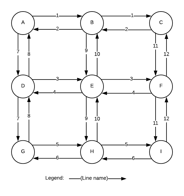
Figure 3: Toy train example

As this is an easy problem, it can be solved using GUROBI solver [25] and compared with the lower bound determined using the Lagrangian relaxation. The iteration process is shown in figure 4. The lower/upper bound after 1000 iterations is (1.4497, 1.4947), while the exact solution of the solver is 1.4947 in the toy problem. The proposed algorithm has a relatively tight bound ($<4\%$) for the toy problem, and the optimal solution is found when solving the upper bound. Therefore, our algorithm can correctly identify the optimal solution in this example.

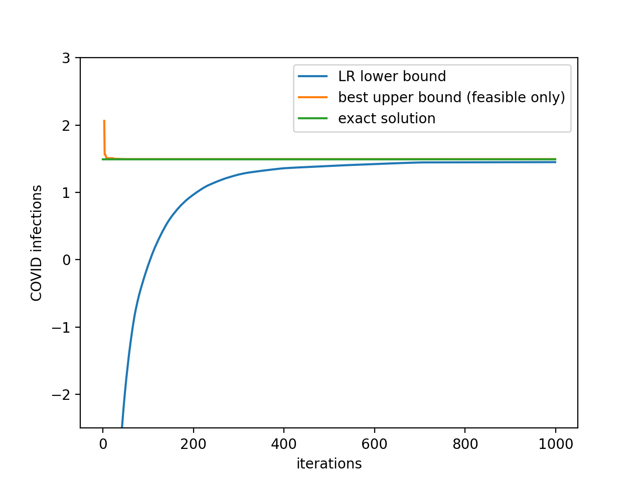
Figure 4: LR iteration of toy example

5.1.3 Sensitivity analysis on budget

When budget is limited, we cannot operate too many train/bus runs. The total number of pandemic infection will increase as we cut the budget (See 5). We can see there is a minimum budget where the model become infeasible, and both of the pandemic cases and the total travel time are more sensitive as the budget level gets closer to this minimum budget (transition point).

To show the impact of budget, we will use the best upper bound result after 1000 LR iterations for different parameters. We set the capacity to be 600. Note that our algorithm is just a heuristic and might not be the actual optimal solution, but just an upper bound.

In this example, when budget is greater than 70% of the total budget provided in the last example, we can see the optimal solution will not change since the budget constrain is loose. When budget is smaller than 70%, the pandemic infection (our objective function) will increase when we cut the budget further. When budget is smaller than 45% of the total budget, the problem could be infeasible, since we cannot find a feasible solution satisfying all demand after 1000 LR iterations. Therefore, the budget transition point is $<45\%$.

Note that the pandemic cases (objective function) is more sensitive when budget level gets smaller (see fig 5 (a)). This is because the LP relaxed lower bound

$F(b):=$ LP relaxed optimal objective function with budget $b$

is convex with respect to $b$. Although the actual optimal objective function is not convex with respect to budget since we have a lot of integer variables, the trend is similar: the new pandemic cases is not sensitive when budget is great, but will be sensitive when budget is small.

For total travel time, we can see in fig 5 (b) that the trend of total travel time is the same as the pandemic cases, even if we don’t have total travel time explicitly in our objective function. This is because the goal to minimize the pandemic contraction coincide with the goal to minimize total passenger travel time (see section 3.7).

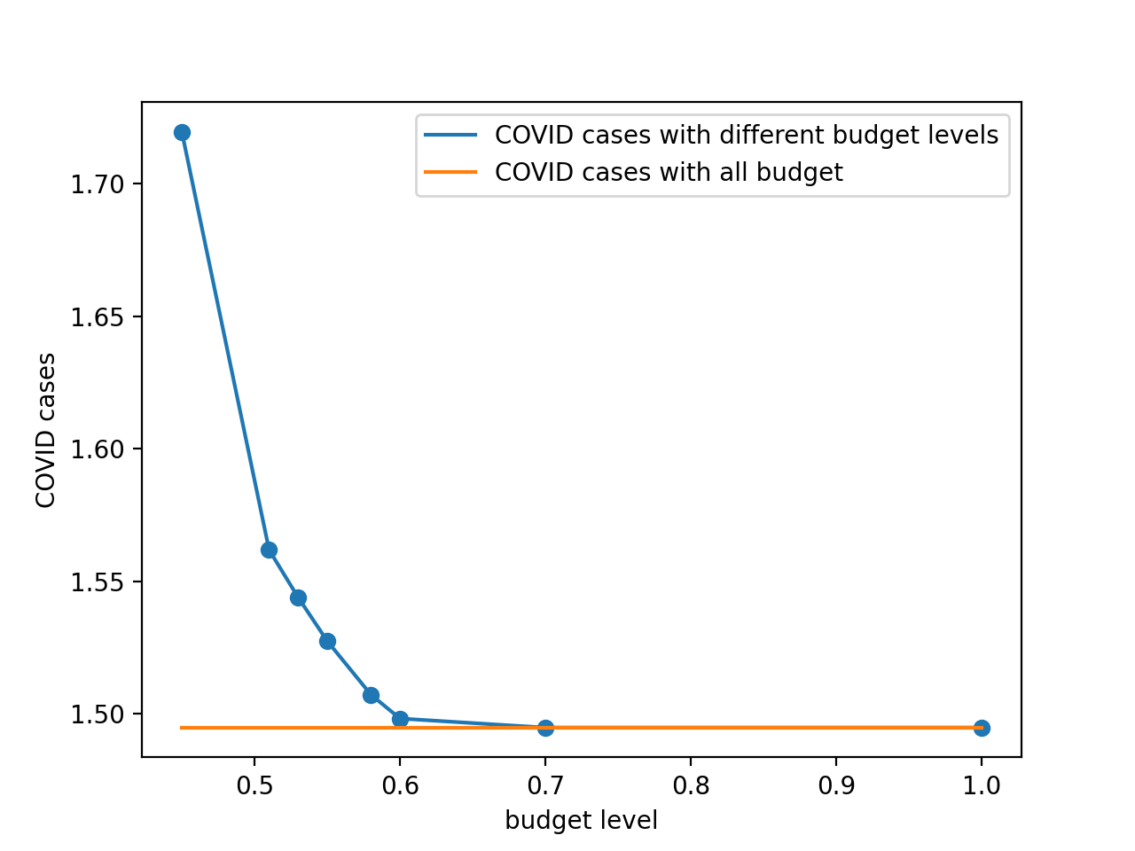
(a) COVID cases

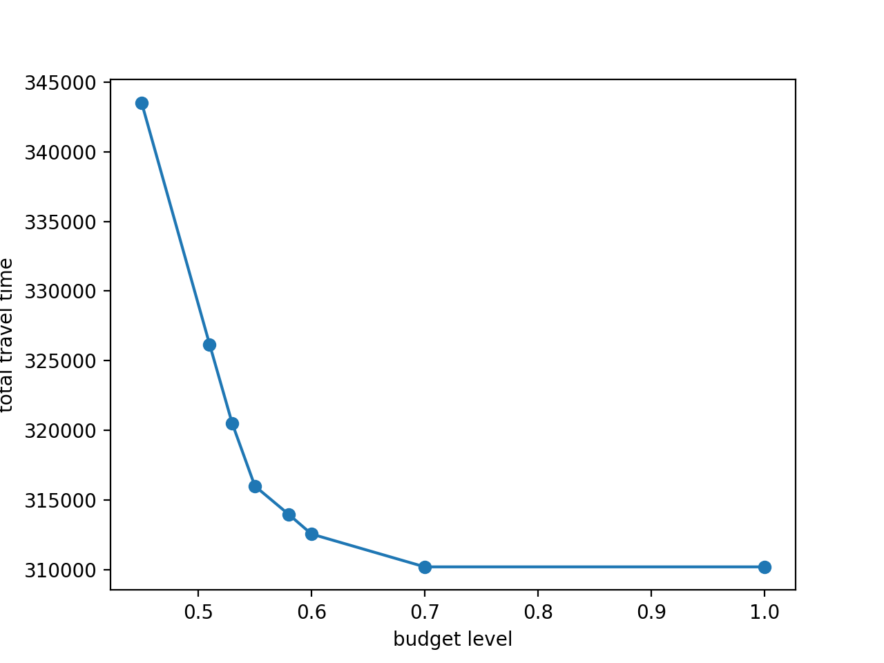
(b) total travel time

Figure 5: Sensitivity analysis on budget

5.1.4 Sensitivity analysis on capacity

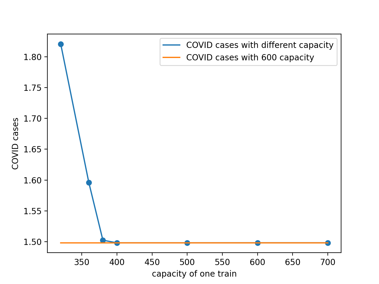
(a) COVID cases

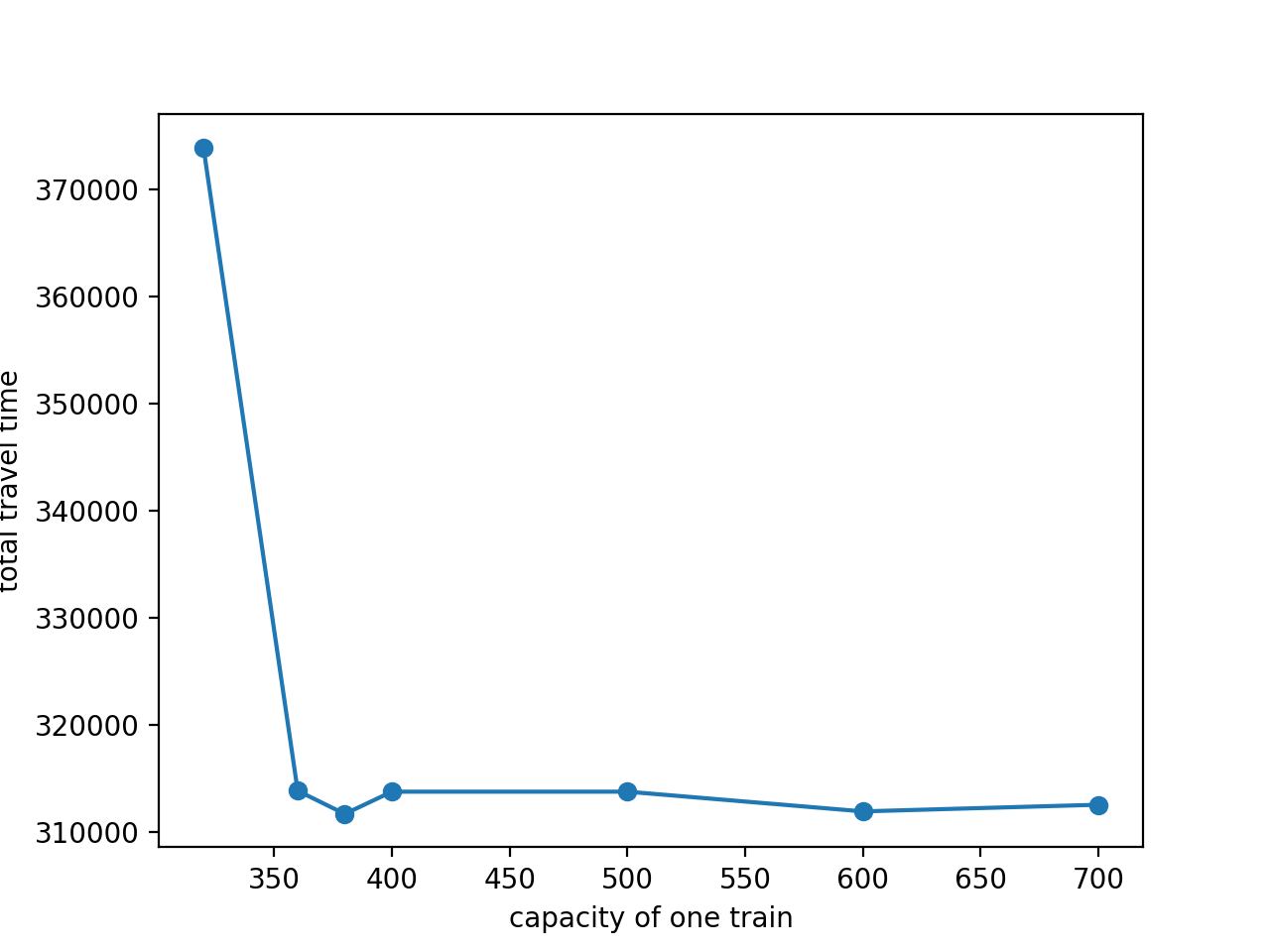
(b) total travel time

Figure 6: Sensitivity analysis on capacity

When the capacity of one train is limited, we need to assign more train runs to the system to satisfy all demand. However, with the budget constraint, the number of open lines and train runs are limited, and the objective function (the number of new cases) will increase when we have smaller capacity for each train.

The trend of the new cases and total travel time are similar to what happens when we change budget: there is a minimum capacity where this problem become infeasible, and both of the new cases and total passenger travel are more sensitive when the capacity gets closer to the minimum capacity.

We change the capacity of one train in this model to see how the new case will change when we have different level of capacity (see fig 6). For each different parameter, we set the budget level to be 60% and did 1000 iterations of our LR algorithm and use the best upper bound as the result. In our experiments, we can see that when capacity is greater or equal to 400, the objective function is the same. While when capacity become less than 320, there is still no feasible solution found after 1000 LR iterations, so the transition point is $<320$. The trend of total travel time is similar, but with some fluctuations since the total travel time is not our objective function but is just positively correlated to the objective (new cases), and we are only using approximated algorithms here.

Also note that the transition point for budget and capacity are correlated. If the budget is smaller then the transition point for capacity is greater. For example, we also did the sensitivity analysis when the budget level is 100%. In this case, the transition point for budget is less than 110, which is much smaller than 320.

5.2 A real world example: BART

5.2.1 Parameters

BART is a rapid transit system that serves the San Francisco Bay Area. It spans 121 miles of double track, consisting of 48 stations[10]. We consider the peak hours operation (7:00–10:00) as the time horizon.

The network is shown in figure [9]. The time horizon is discretized into 1-minute intervals. According to the timetable, it can be observed that the in-vehicle travel time is much longer than the dwell time at each station, so the assumptions are satisfied. There are many parallel links in BART, and transfers are prevalent in this system. The proposed space-time network model can capture all these network features.

The operation cost can be estimated from the BART budget report [9]. The total operating cost budget is 767.8M in 2020. As the operation time of each train dispatch for each line can be calculated, assuming that the operation cost is proportional to the operating time, the cost of one dispatch can be estimated, as shown in Table 2.

Since the demand originated at each station is non-zero, and the walking distance between two stations in BART system is long. We know that we have to open all the lines otherwise the system would be infeasible, since we have strict demand constraints. We set the time tolerance for each user to be $TL=45min$.

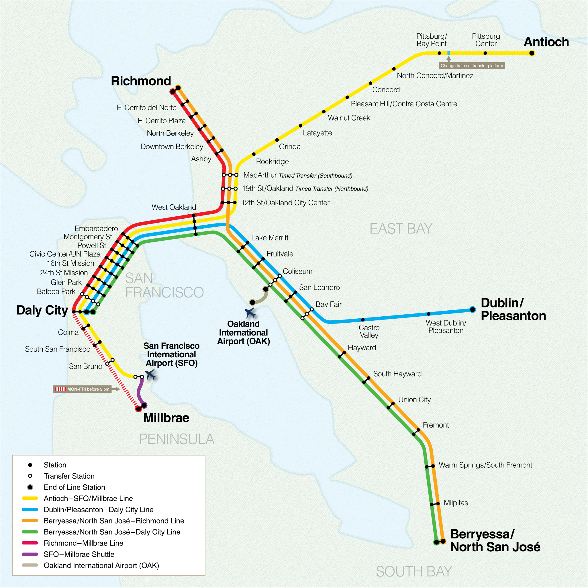
Figure 7: map of BART [9]

Line number	Color	Line name	Cost($)
0	gray	Oakland Airport to Coliseum	848
1	gray	Coliseum to Oakland Airport	848
2	blue	Daly City to Dublin/Pleasanton	4179
3	blue	Dublin/Pleasanton to Daly City	4118
4	green	Daly City to Berryessa/North San Jose	5390
5	green	Berryessa/North San Jose to Daly City	5330
6	orange	Berryessa/North San Jose to Richmond	4966
7	orange	Richmond to Berryessa/North San Jose	5330
8	purple	Millbrae to SFIA	545
9	purple	SFIA to Millbrae	545
10	red	Millbrae/Daly City to Richmond	4361
11	red	Richmond to Daly City/Millbrae	4542
12	yellow	Millbrae/SFIA to Antioch	6299
13	yellow	Antioch to SFIA/Millbrae	6481

Table 2: Line info and cost of one run for different lines

During the pandemic, BART reduced operation in 2020, and now the system is being reopened according to the guidelines [7]. Disinfectants are being sprayed on the surfaces of train cars and station platforms, and face coverings are required at all times for all riders aged 13 and above. According to BART, the capacity of each car is 30 people under the 6-feet social distancing rule. As long trains are in use during the pandemic, each train’s capacity is 600 people. As a platform’s capacity is approximately 1.5 times the train capacity, we use 900 as the platform capacity.

In the current timetable, lines 0 and 1 have high operation frequencies as these two lines are Oakland International Airport shuttles that current employ smaller carts called AirBART. Therefore, the operation pattern is different from the other line and we will ignore the these two lines from Oakland Airport and relocate the demand from Oakland Airport to Coliseum station instead.

Hourly OD demand data from the BART API [8] are used to estimate the intensity of the Poisson flow during the decision time horizon. The demand is aggregated every 20 minutes to reduce the dimensions of the problem. That is, the desired departure time in our time dependent OD matrix must be multiplies of 20 minute, like 0,20,40,60 etc. Here, we consider operation from 8:00AM to 11:00AM. Using the proposed algorithm, the following iteration process is executed. To further simplify the model, train dispatch is only allowed every 10 min, that is, dispatch occurs only at time 8:10, 8:20, and so on.

5.2.2 Optimal timetable design and performance of our algorithm

After plugging the BART network in our model and simplifying the problem by only considering a max frequency of 10 minutes and ignoring Oakland Airport line, we got $277$ 0-1 variables. The number of integer variable $x_{lt}$ is $12\times 6\times 3=216$ since we have 12 lines during a 3-hour time period. And we have one variable for each line and each station.

The number of continuous variables is exponentially many, but we only generate a few of them in our iteration. The network has $22630$ arcs: We have $3888$ links in $\mathcal{A}_{travel}$, and $2398$ links in $\mathcal{A}_{wait}$ using sparse storage of network by only considering time step where there could be an arrival/departure of a train at the platform. Most of the lines will share platforms except at station MacArthur, 19th St Oakland, Coliseum and Balboa Park, we have $71+53+107+125=356$ links in $\mathcal{A}_{transfer}$ where $71,53,107$ and $125$ corresponds to MacArthur, 19th St Oakland, Coliseum and Balboa Park respectively. In addition to these, we have $13000$ links in $\mathcal{A}_{os}$ and $2988$ links in $\mathcal{A}_{sd}$. Noting that a large number of links in $\mathcal{A}_{os}$ and $\mathcal{A}_{sd}$ will not make the algorithm much more difficult to solve since they will not add too much route choice, and we use the path-flow formulation and column generation, which only requires doing one shortest path for each OD pair.

The number of non-zero OD pair is $2800$ as we aggregate demand every $20min$ and most of the time dependent OD matrix is zero. When solving SUB1, we need to find shortest paths for $2800$ OD pairs. We will keep generate paths until all paths satisfying boundedly rational conditions with negative reduced cost is found, so that the number of basis expands quickly. When most of the capacity constraints are not tight, and the network structure is not too complicated like BART, we can find the optimal solution after less than 100 column generation steps. The typical number of columns needed is less than $15000$ in our iterations and we only have at most $|\mathcal{A}_{travel}|+|\mathcal{W}|<5000$ constraints (rows) while most of the capacity constraints are not tight.

We have to admit that if the demand level is high and most of the constraints are tight, this problem can be difficult to solve and we cannot find an feasible solution after many LR iteration steps. This is a limit of our problem. But luckily, for BART system, only some trains reaches their capacity like trains running on cross-bay link, where there is a large flow from east bay to the downtown SF every workday morning.

After 1000 LR iterations, the gap is approximately 5.4%. (LB: 0.470605, UB: 0.496054). The upper bound solution is better than the cost calculated using the current running timetable (cost: 0.500649), which is calculated based on timetable of BART weekday operation[7] using our column generation algorithm to find the optimal network flow and cost.

In the proposed optimal solution, all train lines and stations will be opened. The reason is that we need to cover all stations to have a feasible solution and we must open most of lines in BART system to make sure all stations are covered. Although passengers can walk directly from the origins to stations, the walking distance is great since the distance between two station is quite large in BART system. Therefore, passengers using the system must have access to a station nearby, and we need to open most of the lines to cover all stations. Another reason is given by experiments in section 5.2.3, the optimal design will open all lines once all stations are covered and the timetable become more flexible to reduce the number of new infections.

The optimal timetable is shown in table 3. For example if $x_{2,10}=1$ then we will have one train run dispatched for line 2 at $time=10min$ ($8:10$). It can be seen that most of the trains will have two to four runs per hour in our optimal plan, while the current timetable has only two runs. It can also be observed that lines 11 and 13 (Richmond to Millbrae, and Antioch to SFIA) has much more runs than lines 10 and 12 ( Millbrae to Richmond, and SFIA to Antioch). During the morning peak hour, people need to leave their homes in the East Bay for travel to the San Francisco CBD area, and our design captured this demand pattern.

Compared to the original timetable, our timetable has higher frequency in the first two hours (8:00AM-10:00AM) or (0-120 min). This is because the demand in the first two hours are much higher than the demand from 10:00AM to 11:00AM. In BART data, the total daily demand is 2200 in 8:00-9:00 AM, 1649 in 9:00-10:00AM and 1337 in 10:00-11:00AM.

Another major difference between our timetable and the existing timetable is that we have much fewer operations for line 8 and 9 (Millbrae to SFIA and SFIA to Millbrae). There are two reasons for this: (1). These lines serves only passengers between Millbrae and SFIA, and the number of passengers is small compared to the whole system ($\approx 0.1\%$, with 14.75 passengers from MLBR to SFIA and 15.57 passengers from SFIA to MLBR while the whole system has an average of 27677.38 daily users). (2). Our algorithm favors long distance lines since we assume all trains need to be cleaned after one operation, and the cleaned cost and time is fixed. Therefore, the per-mile cost is higher for short lines compared to other lines, and the algorithm tend to operate long distance lines.

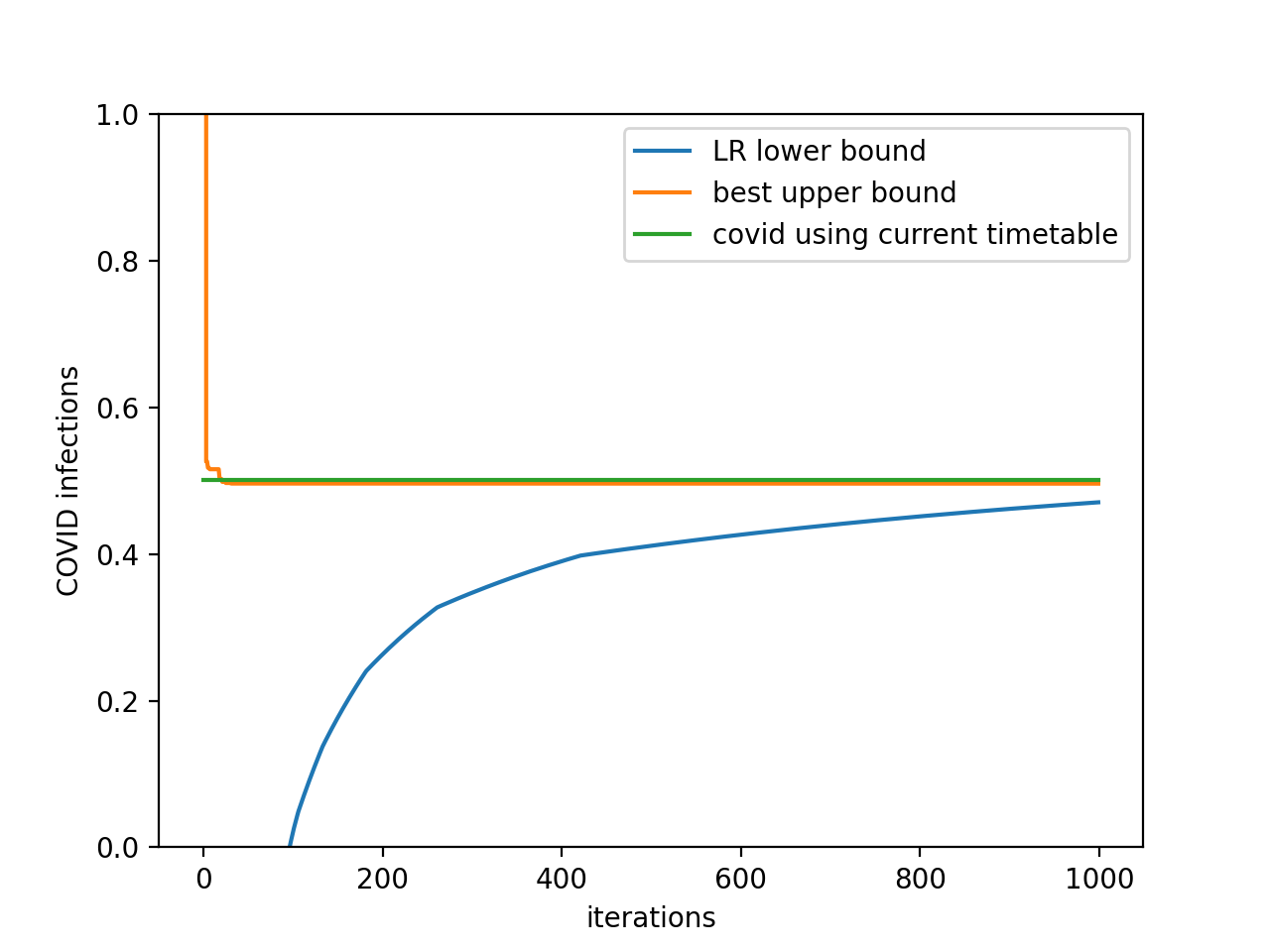
Figure 8: LR iteration of BART example

Line number	Line name	Optimal timetable	Current timetable
2	Daly City to Dublin/Pleasanton	0,40,60,70,80,110,120,150	21,51,81,111,141,171
3	Dublin/Pleasanton to Daly City	10,30,40,70,80,100,120,140	9,39,69,99,129,159
4	Daly City to Berryessa/North San Jose	10,30,40,60,90,110,130	12,42,72,102,132,162
5	Berryessa/North San Jose to Daly City	0,20,40,70,100	0,30,60,90,120,150
6	Berryessa/North San Jose to Richmond	20,40,60,70,90,100,170	12,42,72,102,132,162
7	Richmond to Berryessa/North San Jose	20,30,50,90,110,120,140,150	3,33,63,93,123,153
8	Millbrae to SFIA	40,110	27,57,87,117,147,177
9	SFIA to Millbrae	120,170	9,39,69,99,109,129,159
10	Millbrae/Daly City to Richmond	20,50,70,100	18,48,78,108,138,168
11	Richmond to Daly City/Millbrae	10,30,40,50,80,90,100,130,140,170	9,39,69,99,129,159
12	Millbrae/SFIA to Antioch	20,50,60,70,80,110,120,170	24,54,84,114,144,174
13	Antioch to SFIA/Millbrae	10,20,60,70,80,90,100,120,140,150,170	0,30,60,90,120,150

Table 3: Optimal timetable

5.2.3 What will happen if we close/open lines

From the previous example, we know with the boundedly rational constraints, the problem can be infeasible if we don’t cover all the stations, and given the stations are covered, we will open all lines in the optimal solution. To find out why it is the case and what will happen if we don’t open all the lines or stations. We assume in this experiment that passengers will go to the closest station from their origin and leave the system from the station closest to their destination using the shortest path in the physical network, so the total demand is the same. We open the lines one by one following table 4. The proposed algorithm is then executed for 1000 LR iterations to find the upper/lower bound of the COVID-19 cost, optimal timetable design, and network flow assignment for each experiment. The resulting objective function (new cases), total travel time inside and outside the transit system are shown in table 5.

Experiment number	Yellow	Blue	Green	Orange	Red	Purple
0	✓
1	✓	✓
2	✓	✓	✓
3	✓	✓	✓	✓
4	✓	✓	✓	✓	✓
5	✓	✓	✓	✓	✓	✓

Table 4: Line opened in each experiment

Experiment number	0	1	2	3	4	5
New cases	infeasible	0.42663942	0.46613135	0.61159565	0.5661387	0.49605433
Travel time in the system	infeasible	60734	66413	86091	80032	70073
Travel time outside the system	infeasible	14134	9057	336	216	0
Line 2 runs	infeasible	14	12	13	6	8
Line 3 runs	infeasible	15	12	13	2	9
Line 4 runs	infeasible	0	9	2	10	9
Line 5 runs	infeasible	0	12	3	13	5
Line 6 runs	infeasible	0	0	13	13	7
Line 7 runs	infeasible	0	0	3	10	8
Line 8 runs	infeasible	0	0	0	0	2
Line 9 runs	infeasible	0	0	0	0	2
Line 10 runs	infeasible	0	0	0	4	4
Line 11 runs	infeasible	0	0	0	4	11
Line 12 runs	infeasible	17	14	14	2	9
Line 13 runs	infeasible	17	17	7	15	11

Table 5: What happens when we close some lines

From table 5, we can see when we only open two lines, the demand is huge and we cannot satisfy all the demand in experiment 0. As we expand the number of lines, more stations are covered, the travel cost outside the system (time it takes for passengers to travel from origins to stations and from stations to destinations) will decrease, and the number of train runs needed for each line decreases since we don’t rely solely one these lines after opening new lines. Also, we notice that the new cases or travel cost inside the system is not monotone. It depends on the network structure.

1. When we only open a small fraction of lines, not all stations are covered and many people spend most of their time walking outside the system. Therefore, the number of new infection inside the system is small. At this time, opening a new line result in a increase in demand with respect to passenger distance traveled, and the objective function (new cases) will also increase.

2. When we have the most of the network opened, all the stations are covered and we have many parallel lines. These features enable us to make flexible timetables and the optimal new infection number is small. At this time, if we close some existing lines and stations, passengers will go to nearby opened stations and the number of queuing passengers waiting will increase, leading to more infections. In addition, if we close parallel lines in the system, the designed capacity between two stations are less flexible and leads to an increase in both total travel time and the waiting time on platforms, thus increasing the number of infections. This also explained why all lines are opened in the optimal design from section 5.2.2

6 Conclusions and future research

In this study, we combined a simplified SCME model and a space-time dynamic transit network to estimate the impact of the pandemic on the public transit system. The proposed model can predict new the pandemic cases in any transit system. We also developed an algorithm to find the optimal network reopening plan and timetable simultaneously, considering the risk of pandemic infection and social distancing rules. The proposed model and the Lagrangian relaxation frame can also be extended to other economics problems where reopening too quickly under pandemic conditions may result in a ’second wave’ of the pandemic.

Based on the numerical example, it can be observed that the proposed algorithm can provide a relatively good lower and upper bounds for the design problem. However, we also notice that this algorithm can only solve relative simple problem where not too many capacity constraints are tight, otherwise the column generation will take a long time and the number of variables explodes.

From the experiments, we know that the sensitivity of budget and capacity constraints are correlated. With capacity fixed, there is a transition point for budget where the problem become infeasible if budget is smaller than this point, and both new infection number and travel time are more sensitive as budget gets closer to this transition point. Similar phenomena holds for capacity with budget fixed. In addition, with more budget, the transition point of capacity become smaller and the number of new cases is less sensitive with respect to capacity.

We also know that if we assume people who need the public transportation system will go to the closest opened station and keep using the system. Then we should either (1) open as many lines as possible and operate parallel lines, so that the system has enough flexibility to deal with time and space dependent travel demand and control the spread of the disease, or (2) only operate a small number of lines so that people are forced outside the system to prevent infections. It is not wise to cover many stations with only small number of lines. In that case, we will keep most of the demand in the system while we cannot deal with this demand with many lines closed.

Our future research will consider the dynamics in stochastic demand modeling. In the current model, the OD demand is deterministic and must be given in constraints 11. This means that if one OD pair relies on one particular line, then this line must be opened with the optimal design. In contrast, some demand may be sacrificed to decrease the risk of the pandemic. Furthermore, the demand itself is a stochastic process (possibly Markovian) following specific transition models. It is possible to design a non-myopic network reopening plan for each period during the entire reopening phase.

References

- Acemoglu et al. [2020] Acemoglu, D., Chernozhukov, V., Werning, I., Whinston, M.D., 2020. A multi-risk SIR model with optimally targeted lockdown. Report 0898-2937. National Bureau of Economic Research.
- ACtransit [2020] ACtransit, 2020. URL: http://www.actransit.org/2020/04/17/ac-transit-service-updates-related-to-the-coronavirus-covid-19/.
- Allen et al. [2008] Allen, L.J., Brauer, F., Van den Driessche, P., Wu, J., 2008. Mathematical epidemiology. volume 1945. Springer.
- Alvarez et al. [2020] Alvarez, F.E., Argente, D., Lippi, F., 2020. A simple planning problem for covid-19 lockdown. Report 0898-2937. National Bureau of Economic Research.
- An and Lo [2016] An, K., Lo, H.K., 2016. Two-phase stochastic program for transit network design under demand uncertainty. Transportation Research Part B: Methodological 84, 157–181. doi:10.1016/j.trb.2015.12.009.
- APTA [2020] APTA, 2020. URL: https://www.apta.com/public-transit-response-to-coronavirus/.
- BART [2020a] BART, 2020a. URL: https://www.bart.gov/news/articles/2020/news20200526.
- BART [2020b] BART, 2020b. URL: https://www.bart.gov/about/reports/ridership.
- BART [2021] BART, 2021. URL: (http://api.bart.gov/.
- Bay Area Rapid Transit (2019) [BART] Bay Area Rapid Transit (BART), 2019. San Francisco Bay Area Rapid Transit District Adopted Budget Fiscal Year 2020. Report. BART. URL: https://www.bart.gov/sites/default/files/docs.
- Birge et al. [2020] Birge, J.R., Candogan, O., Feng, Y., 2020. Controlling epidemic spread: Reducing economic losses with targeted closures .
- Brauer et al. [2019] Brauer, F., Castillo-Chavez, C., Feng, Z., 2019. Mathematical models in epidemiology. Springer.
- Cancela et al. [2015] Cancela, H., Mauttone, A., Urquhart, M.E., 2015. Mathematical programming formulations for transit network design. Transportation Research Part B: Methodological 77, 17–37. doi:10.1016/j.trb.2015.03.006.
- CDC [2020a] CDC, 2020a. Covid-19: Frequently asked questions. URL: https://www.cdc.gov/coronavirus/2019-ncov/faq.html.
- CDC [2020b] CDC, 2020b. Covid-19: How it spreads. URL: https://www.cdc.gov/coronavirus/2019-ncov/faq.html.
- CDC [2020c] CDC, 2020c. Covid-19: using transportatoin: Public transit, rideshares and taxis, micro-mobility devices, and personal vehicles. URL: https://www.cdc.gov/coronavirus/2019-ncov/daily-life-coping/using-transportation.html.
- Chinazzi et al. [2020] Chinazzi, M., Davis, J.T., Ajelli, M., Gioannini, C., Litvinova, M., Merler, S., y Piontti, A.P., Mu, K., Rossi, L., Sun, K., 2020. The effect of travel restrictions on the spread of the 2019 novel coronavirus (covid-19) outbreak. Science 368, 395–400.
- Fan et al. [2018] Fan, W., Mei, Y., Gu, W., 2018. Optimal design of intersecting bimodal transit networks in a grid city. Transportation Research Part B: Methodological 111, 203–226. doi:10.1016/j.trb.2018.03.007.
- Farahani et al. [2013] Farahani, R.Z., Miandoabchi, E., Szeto, W.Y., Rashidi, H., 2013. A review of urban transportation network design problems. European Journal of Operational Research 229, 281–302. doi:10.1016/j.ejor.2013.01.001.
- Frost [2020] Frost, M., 2020. New york city subway ridership down 92 percent due to coronavirus. URL: https://brooklyneagle.com/articles/2020/04/08/new-york-city-subway-ridership-down-92-percent-due-to-coronavirus/.
- Gao et al. [2004] Gao, Z., Sun, H., Shan, L.L., 2004. A continuous equilibrium network design model and algorithm for transit systems. Transportation Research Part B: Methodological 38, 235–250. doi:10.1016/s0191-2615(03)00011-0.
- Gershon et al. [2020] Gershon, D., Lipton, A., Levine, H., 2020. Managing covid-19 pandemic without destructing the economy. arXiv 10324.
- Glover et al. [2020] Glover, A., Heathcote, J., Krueger, D., Ríos-Rull, J.V., 2020. Health versus wealth: On the distributional effects of controlling a pandemic. Report 0898-2937. National Bureau of Economic Research.
- Guihaire and Hao [2008] Guihaire, V., Hao, J.K., 2008. Transit network design and scheduling: A global review. Transportation Research Part A: Policy and Practice 42, 1251–1273. doi:10.1016/j.tra.2008.03.011.
- GUROBI [2020] GUROBI, 2020. URL: http://www.gurobi.com.
- Ibarra-Rojas et al. [2015] Ibarra-Rojas, O.J., Delgado, F., Giesen, R., Muñoz, J.C., 2015. Planning, operation, and control of bus transport systems: A literature review. Transportation Research Part B: Methodological 77, 38–75. doi:10.1016/j.trb.2015.03.002.
- Ives and Bozzuto [2020] Ives, A.R., Bozzuto, C., 2020. State-by-state estimates of r0 at the start of covid-19 outbreaks in the usa. medRxiv , 2020.05.17.20104653doi:10.1101/2020.05.17.20104653.
- JHU [2020] JHU, 2020. URL: https://coronavirus.jhu.edu/.
- Jia et al. [2020] Jia, J.S., Lu, X., Yuan, Y., Xu, G., Jia, J., Christakis, N.A., 2020. Population flow drives spatio-temporal distribution of covid-19 in china. Nature 582, 389–394. URL: https://doi.org/10.1038/s41586-020-2284-y, doi:10.1038/s41586-020-2284-y.
- Joselow [2020] Joselow, M., 2020. There is little evidence that mass transit poses a risk of coronavirus outbreaks. Scientific American .
- Kaplan [2020] Kaplan, E.H., 2020. Covid-19 scratch models to support local decisions. Manufacture and Service Operations Management 22, 645–655.
- Kumar et al. [2021] Kumar, P., Khani, A., Lind, E., Levin, J., 2021. Modeling epidemic spreading through public transit using time-varying encounter network. Transportation Research Record .
- Li et al. [2020] Li, R., Pei, S., Chen, B., Song, Y., Zhang, T., Yang, W., Shaman, J., 2020. Substantial undocumented infection facilitates the rapid dissemination of novel coronavirus (sars-cov-2). Science 368, 489–493.
- Liu and Zhou [2016] Liu, J., Zhou, X., 2016. Capacitated transit service network design with boundedly rational agents. Transportation Research Part B: Methodological 93, 225–250. doi:10.1016/j.trb.2016.07.015.
- Liu et al. [2020] Liu, K., Yin, L., Ma, Z., Zhang, F., Zhao, J., 2020. Investigating physical encounters of individuals in urban metro systems with large-scale smart card data. Physica A: Statistical Mechanics and its Applications 545.
- Luo et al. [2020] Luo, K., Lei, Z., Hai, Z., Xiao, S., Rui, J., Yang, H., Jing, X., Wang, H., Xie, Z., Luo, P., Li, W., Li, Q., Tan, H., Xu, Z., Yang, Y., Hu, S., Chen, T., 2020. Transmission of sars-cov-2 in public transportation vehicles: A case study in hunan province, china. Open Forum Infectious Diseases 7. URL: https://doi.org/10.1093/ofid/ofaa430, doi:10.1093/ofid/ofaa430, arXiv:https://academic.oup.com/ofid/article-pdf/7/10/ofaa430/34006085/ofaa430.pdf. ofaa430.
- Martcheva [2015] Martcheva, M., 2015. An introduction to mathematical epidemiology. volume 61. Springer.
- Mo et al. [2021] Mo, B., Feng, K., Shen, Y., Tam, C., Li, D., Yafeng, Y., Jinhua, Z., 2021. Modeling epidemic spreading through public transit using time-varying encounter network. Transportation Research Part C: Emerging Technologies 122.
- Niu and Zhou [2013] Niu, H., Zhou, X., 2013. Optimizing urban rail timetable under time-dependent demand and oversaturated conditions. Transportation Research Part C: Emerging Technologies 36, 212–230. doi:10.1016/j.trc.2013.08.016.
- Niu et al. [2015] Niu, H., Zhou, X., Gao, R., 2015. Train scheduling for minimizing passenger waiting time with time-dependent demand and skip-stop patterns: Nonlinear integer programming models with linear constraints. Transportation Research Part B: Methodological 76, 117–135. doi:10.1016/j.trb.2015.03.004.
- Sadik-Khan and Solomonow [2020] Sadik-Khan, J., Solomonow, S., 2020. Fear of public transit got ahead of the evidence. The Atlantic .
- Sanche et al. [2020] Sanche, S., Lin, Y.T., Xu, C., Romero-Severson, E., Hengartner, N., Ke, R., 2020. High contagiousness and rapid spread of severe acute respiratory syndrome coronavirus 2. Emerging Infectious Diseases 26, 1470–1477. doi:https://dx.doi.org/10.3201/eid2607.200282.
- Sante Publique France [2020] Sante Publique France, 2020. Covid-19 : point épidémiologique du 4 juin 2020. URL: https://www.santepubliquefrance.fr/maladies-et-traumatismes/maladies-et-infections-respiratoires/infection-a-coronavirus/documents/bulletin-national/covid-19-point-epidemiologique-du-4-juin-2020.
- Shen et al. [2020] Shen, Y., Li, C., Dong, H., Wang, Z., Martinez, L., Sun, Z., Handel, A., Chen, Z., Chen, E., Ebell, M.H., Wang, F., Yi, B., Wang, H., Wang, X., Wang, A., Chen, B., Qi, Y., Liang, L., Li, Y., Ling, F., Chen, J., Xu, G., 2020. Community Outbreak Investigation of SARS-CoV-2 Transmission Among Bus Riders in Eastern China. JAMA Internal Medicine 180, 1665–1671. URL: https://doi.org/10.1001/jamainternmed.2020.5225, doi:10.1001/jamainternmed.2020.5225, arXiv:https://jamanetwork.com/journals/jamainternalmedicine/articlepdf/2770172/jamainternal_shen_2020_oi_200076_1611345809.71283.pdf.
- Szeto and Jiang [2014] Szeto, W.Y., Jiang, Y., 2014. Transit route and frequency design: Bi-level modeling and hybrid artificial bee colony algorithm approach. Transportation Research Part B: Methodological 67, 235–263. doi:10.1016/j.trb.2014.05.008.
- The People’s Government of Hubei Province [2020] The People’s Government of Hubei Province, 2020. Wuhan public transport will officially provide commuter services from march 16. URL: https://www.hubei.gov.cn/zhuanti/2020/gzxxgzbd/sz/202003/t20200315_2182086.shtml.
- Verbas and Mahmassani [2015] Verbas, I.O., Mahmassani, H.S., 2015. Integrated frequency allocation and user assignment in multimodal transit networks. Transportation Research Board 2498, 37–45. URL: https://dx.doi.org/10.3141/2498-05, doi:10.3141/2498-05.