Spectral density of individual trajectories of an active Brownian particle

Abstract

We study analytically the single-trajectory spectral density (STSD) of an active Brownian motion as exhibited, for example, by the dynamics of a chemically-active Janus colloid. We evaluate the standardly-defined spectral density, i.e. the STSD averaged over a statistical ensemble of trajectories in the limit of an infinitely long observation time $T$, and also go beyond the standard analysis by considering the coefficient of variation $\gamma$ of the distribution of the STSD. Moreover, we analyse the finite-$T$ behaviour of the STSD and $\gamma$, determine the cross-correlations between spatial components of the STSD, and address the effects of translational diffusion on the functional forms of spectral densities. The exact expressions that we obtain unveil many distinctive features of active Brownian motion compared to its passive counterpart, which allow to distinguish between these two classes based solely on the spectral content of individual trajectories.

Keywords: Active Brownian particle, individual trajectories, spectral density

1 Introduction

Active matter encompasses a variety of systems that are driven locally out of equilibrium, at the scale of each constituents. Most commonly, these active particles consume energy to self-propel and are found across scales, from macroscopic animals forming, e.g., bird flocks [1] or fish schools [2] to the microscopic world where motile bacteria [3] or self-propelled colloids operate [4, 5]. The strong nonequilibrium driving is responsible for a host of collective behaviours with no equilibrium counterpart such as flocking [6], motility-induced phase separation [7] or the so-called bacterial turbulence [8] to name just a few prominent ones.

Active systems have received considerable attention from physicists in the last few decades for the theoretical and practical challenges that they pose [9, 10]. Even at the level of a single active particle, one encounters a rich phenomenology with non-Boltzmann stationary states [11, 12, 13], complex interactions with boundaries [14, 15] and the generic impossibility to define state functions such as pressure [16] or temperature [17].

Two main models have been used for the motion of an active particle. In a first one, run-and-tumble particles (RTPs) alternate periods of directional swimming with short-duration “tumbles” during which they randomise their direction of motion. That model accounts for the trajectories of bacteria like Escherichia coli [3, 18]. In the other class of models, particles self-propel in a direction that fluctuates because of rotational noise. These active Brownian particles (ABPs) [19] are appropriate to describe, for example, Janus colloidal particles decorated with a catalytic patch which prompts a chemical reaction in the surrounding solution [20, 21]. The reaction then generates gradients of product species across the surface of the particle leading to a non-zero self-propulsive force $F$ (see, e.g. Refs. [22, 23]). Within the last decade, various characteristics including the position probability density functions, the marginal distributions and the first-passage properties have been studied for both RTPs [24, 25, 26, 27, 28, 29, 30, 31, 32, 33] and ABPs [34, 35, 36, 37, 38, 39]. In addition, note that many other models of active particles have been proposed [40, 41, 42].

Here, we will focus on the dynamics of an active Brownian particle in the two-dimensional $(x,y)$-plane (see Fig. 2), which is realised experimentally, e.g., in a situation in which a Janus colloid has sedimented on a bottom plate or is trapped at the interface separating two distinct liquids [43, 44] and is therefore restricted to 2d motion. For simplicity, we assume that the rotational diffusion also takes place in the plane which may or may not be the case depending on the experimental setup. Finally, we neglect translational (passive) diffusion which is often very small compared to the active motion. Within these approximations, the system of equations describing the time-evolution of the components $x(t)$ and $y(t)$ of the position of an ABP can be written

$$\dot{x}(t) =v\cos\theta(t)\,,\quad x(0)=0\,,$$ (1)

$$\dot{y}(t) =v\sin\theta(t)\,,\quad y(0)=0\,,$$

where the dot denotes time derivative, $v$ is the constant self-propulsion velocity and $\theta(t)$ is the instantaneous polar angle defining the direction of motion, i.e. the angle between the velocity vector and the $x$-axis. For an ABP, $\theta$ changes due to rotational diffusion so that this process is a one-dimensional Brownian motion (BM) with zero mean and covariance

$$\langle\theta(t_{1})\theta(t_{2})\rangle=\frac{2}{\tau_{R}}\,{\rm min}\left(t_{1},t_{2}\right)\,,$$ (2)

with $\tau_{R}$ the persistence time of the particle, the characteristic time after which the initial orientation is forgotten. Here and in the rest of the paper, the angle brackets denote averaging with respect to different realisations of $\theta(t)$ and we choose the initial condition $\theta(t=0)=0$.

Note that two salient features of the model in Eqs.(1)-(2) are that a) the effective noise is a non-linear function of the random process $\theta(t)$ and b) the components of the instantaneous velocity ($v_{x}(t)=\dot{x}(t)$ and $v_{y}(t)=\dot{y}(t)$) obey

$$v^{2}_{x}(t)+v^{2}_{y}(t)\equiv v^{2}$$ (3)

at any moment in time $t$, which shows explicitly that the components are coupled. These two circumstances clearly entail departures from a standard BM behaviour at some transient stages (see, e.g., Refs. [35, 36, 46, 37, 38, 39] and below). However, as can be expected intuitively, on large time scales the ABP follows a standard two-dimensional BM with an effective diffusion coefficient $D_{e}=v^{2}\tau_{R}/2$ [47]. Note that it remains true even if the particle is placed in an external potential, provided the variations of the potential are small on the scale of the persistence length $l_{p}=v\tau_{R}$ [17].

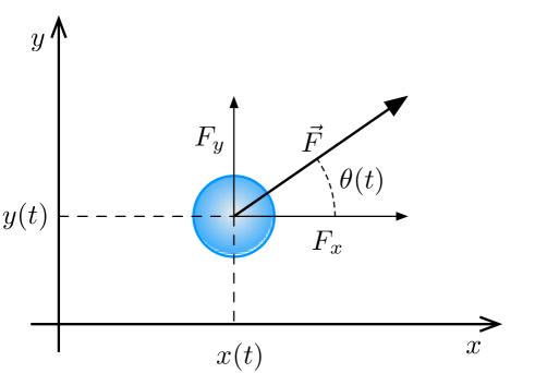
Figure 1: An active colloid on a two-dimensional $(x,y)$-plane. The vector $\vec{F}$ (with components $F_{x}$ and $F_{y}$) denotes the self-propulsion force emerging due to interactions with the environment. $x(t)$ and $y(t)$ are the coordinates of the instantaneous position of the centre of the colloid.

In this paper, we are interested in the power spectral density of an ABP, an aspect that has heretofore not been investigated. It is well-known that the power spectral density of any stochastic process embodies a wealth of information on its temporal evolution and correlations. As such, it is one of the most widely used characterisation tools, and nowadays a substantial knowledge about spectral densities of a variety of processes has been accumulated (see, e.g., Refs. [48, 49, 50, 51, 52, 53, 54, 55, 56, 57] and references therein).

According to the standard definition, the power spectral density $\mu_{x}(f)$ of the process $x(t)$ at frequency $f$ involves taking a statistical average over realisations of the process and the limit of an infinitely long trajectory. For a single trajectory of duration $T$, one defines the single trajectory spectral density (STSD)

$$S_{x}(f,T)=\frac{1}{T}\left|\int_{0}^{T}\textrm{d}t\,e^{ift}\,x(t)\right|^{2}\,,$$ (4)

which is a functional of the trajectory and itself a random process. We denote its average by $\mu_{x}(f,T)=\langle S_{x}(f,T)\rangle$ so that the spectral density is obtained as

$$\mu_{x}(f)=\lim_{T\to\infty}\mu_{x}(f,T)\,.$$ (5)

We note that a standard textbook analysis focuses precisely on $\mu_{x}(f)$ which is an ensemble-averaged property that can be understood as a suitable Fourier transform of the covariance function of the process $x(t)$. In some instances, however, the limit $T\to\infty$ does not exist (see, e.g., Refs. [48, 49, 50, 51, 52, 53, 55, 56, 57] for some examples) and one has to resort to either alternative definitions of the spectral density (e.g. the one due to Wigner and Ville, see Refs. [48, 56] and references therein), or operate directly with the finite-$T$ counterpart $\mu_{x}(f,T)$. Indeed, this quantity is well-defined for any finite $T$ and also gives access to useful information about the ageing properties ($T$-dependence) of spectral densities [58, 59, 60, 61, 62, 63]. In particular, $\mu_{x}(f,T)$ evaluated at zero frequency reads

$$\mu_{x}(f=0,T)=\frac{1}{T}\left\langle\left(\int^{T}_{0}\textrm{d}t\,x(t)\right)^{2}\right\rangle\,,$$ (6)

which is the averaged squared area under random curve $x(t)$ on the interval $t\in(0,T)$ divided by $T$. Observing the rate at which $\mu_{x}(f=0,T)$ diverges, when it does, as $T$ tends to infinity, tells us much about the process itself [55, 58, 59, 60, 61].

Going beyond the standard definition, recent works investigated the statistical properties of the STSD $S_{x}(f,T)$ and calculated its full probability density function for several Gaussian processes [58, 59, 60, 61]. It was realised that the coefficient of variation of this distribution, defined formally by

$$\gamma=\gamma(f,T)=\frac{\sqrt{\langle S^{2}_{x}(f,T)\rangle-\mu^{2}_{x}(f,T)}}{\mu_{x}(f,T)}\,,$$ (7)

is an important characteristic parameter. By definition, it measures the relative amplitude of fluctuations of the STSD at given $f$ and $T$ with respect to its mean value, and hence, shows how representative of the actual behaviour $\mu_{x}(f,T)$ is. It was shown in Refs. [58, 59, 60, 61] that for several known Gaussian processes the coefficient of variation obeys for any $f$ and $T$ a two-sided inequality: $1\leq\gamma\leq\sqrt{2}$, implying that fluctuations of the STSD are generically bigger than the mean value, and hence that large statistical samples are necessary to reliably evaluate $\mu_{x}(f,T)$ in practice. Next, even when the asymptotic behaviours of $\mu_{x}(f)$ are the same for distinctly different processes, it appears that the values of $\gamma$ may be very different, thus allowing to distinguish between different processes. In particular, for the so-called fractional BM (fBM) with Hurst index $H$ — a family of anomalous diffusions — $\mu_{x}(f)\sim 1/f^{2}$ in the limit $f\to\infty$ for standard BM $(H=1/2)$ as well as any super-diffusive fBm with $H>1/2$ [59]. On the contrary, $\gamma$ behaves differently in the two cases: as $f\to\infty$, it approaches a universal value $\sqrt{2}$ for super-diffusion and the value $\sqrt{5}/2$ for standard BM. For sub-diffusive fractional BM the behaviour is again different: $\gamma\to 1$ as $f\to\infty$ [59]. Correspondingly, the analysis of $\gamma$ (in addition to the more commonly used analysis of the mean-squared displacement), provides a robust criterion for anomalous diffusion.

At present, neither the form of the standard power spectral density $\mu_{x}(f)$, nor its ageing properties or the behaviour of the characteristic parameter $\gamma$ are known for the much popular ABP model. We bridge this gap by evaluating explicit expressions for these characteristic properties, discuss their similarity to those of standard BM and emphasise several distinctive features. We also address additional questions about the cross-correlations of the STSD for the $x$- and $y$-components, and about the effects of translational diffusion. The paper is organised as follows: in Sec. 2 we first evaluate the exact form of the standard textbook power spectral density of trajectories of an ABP in the limit of an infinite observation time before discussing some features of the finite-$T$ case. Sec. 3 is devoted to the analysis of the coefficient of variation $\gamma$ associated with the random functionals $S_{x}(f,T)$ and $S_{y}(f,T)$ both in the limit $T\to\infty$ and for finite $T$. We also analyse at the end of Sec. 3 the behaviour of the Pearson correlation coefficient for $S_{x}(f,T)$ and $S_{y}(f,T)$. In Sec. 4 we study the effects of translational diffusion on the STSD before concluding in Sec. 5 with a brief recapitulation of our results.

2 Power spectral density of trajectories of an active Brownian particle

2.1 Position correlation functions

Computing the standard power spectral density $\mu_{x}(f)$ and $\mu_{y}(f)$ necessitates only the knowledge of the two-time correlation functions $C_{xx}(t_{1},t_{2})=\langle x(t_{1})x(t_{2})\rangle$ and $C_{yy}(t_{1},t_{2})=\langle y(t_{1})y(t_{2})\rangle$. These can be determined directly from Eqs.(1)-(2), which we show explicitly here for $x(t)$.

We first differentiate $C_{xx}$ about $t_{1}$ and $t_{2}$ giving

$$\frac{\partial^{2}C_{xx}(t_{1},t_{2})}{\partial t_{1}\partial t_{2}}=v^{2}\langle\cos\theta(t_{1})\cos\theta(t_{2})\rangle\,.$$ (8)

Applying the Itō formula [64] to differentiate $\cos^{2}\theta(t)$ we obtain

$$\frac{d}{dt}\langle\cos^{2}\theta(t)\rangle=-\frac{\langle 2-4\cos^{2}\theta(t)\rangle}{\tau_{R}}$$ (9)

which integrates to

$$\langle\cos^{2}\theta(t)\rangle=\frac{1}{2}\left(1+e^{-4t/\tau_{R}}\right)\,.$$ (10)

Applying again the Itō formula to differentiate $\cos\theta(t_{1})\cos\theta(t_{2})$ with respect to $t_{1}$ and integrating gives for the correlator

$$\langle\cos\theta(t_{1})\cos\theta(t_{2})\rangle=\frac{1}{2}\left(1+e^{-4t/\tau_{R}}\right)e^{-(t_{1}-t_{2})/\tau_{R}}.$$ (11)

Finally, integrating Eq. (11) over $t_{1}$ and $t_{2}$ gives the correlation for $x$ (and similarly for $y$)

$$C_{xx}(t_{1},t_{2})=v^{2}\tau_{R}^{2}\biggl{[}\frac{t_{2}}{\tau_{R}}-\frac{1}{4}+\frac{1}{3}e^{-t_{1}/\tau_{R}}+\frac{1}{3}e^{-t_{2}/\tau_{R}}-\frac{1}{12}e^{-4t_{2}/\tau_{R}}$$ (12)

$$-\frac{1}{2}e^{-(t_{1}-t_{2})/\tau_{R}}+\frac{1}{6}e^{-(t_{1}+3t_{2})/\tau_{R}}\biggr{]}\,,$$

$$C_{yy}(t_{1},t_{2})=v^{2}\tau_{R}^{2}\biggl{[}\frac{t_{2}}{\tau_{R}}-\frac{3}{4}+\frac{2}{3}e^{-t_{1}/\tau_{R}}+\frac{2}{3}e^{-t_{2}/\tau_{R}}+\frac{1}{12}e^{-4t_{2}/\tau_{R}}$$

$$-\frac{1}{2}e^{-(t_{1}-t_{2})/\tau_{R}}-\frac{1}{6}e^{-(t_{1}+3t_{2})/\tau_{R}}\biggr{]}\,,$$

where we assumed without loss of generality that $t_{1}\geq t_{2}$. One can also directly read off from Eqs.(12) the exact expressions for the mean-squared displacements of the components at time $t$:

$$\langle x^{2}(t)\rangle =v^{2}\tau_{R}^{2}\biggl{[}\tau-\frac{3}{4}+\frac{2}{3}e^{-\tau}+\frac{1}{12}e^{-4\tau}\biggr{]}\,,$$ (13)

$$\langle y^{2}(t)\rangle =v^{2}\tau_{R}^{2}\biggl{[}\tau-\frac{5}{4}+\frac{4}{3}e^{-\tau}-\frac{1}{12}e^{-4\tau}\biggr{]}\,,$$

where we introduced the dimensionless time variable $\tau=t/\tau_{R}$.

From Eq. (13), we see that, at long times $t/\tau_{R}\to\infty$, the differences between $x$ and $y$ due to the initial condition are forgotten and both $\langle x^{2}(t)\rangle$ and $\langle y^{2}(t)\rangle$ grow linearly in time, indicating a diffusive motion with an effective diffusion coefficient

$$D_{e}=\frac{v^{2}\tau_{R}}{2}\,,$$ (14)

as derived previously in [47]. At short times, $x(t)$ and $y(t)$ behave differently: $\langle x^{2}(t)\rangle\simeq v^{2}t^{2}$, i.e. it exhibits a simple ballistic motion with the velocity $v$, while $\langle y^{2}(t)\rangle$ grows faster with time at this initial stage, $\langle y^{2}(t)\rangle\simeq 2v^{2}t^{3}/(3\tau_{R})$.

Plugging the expressions of the correlators Eq.(12) into Eq. (4) and performing the two-fold integral allows to compute $\mu_{x}(f,T)$ and $\mu_{y}(f,T)$ explicitly. We give this exact form in the infinite-trajectory limit in the next subsection. We omit the lengthy expression for arbitrary $T$ but discuss limiting situations at finite $T$ in Sec. 2.3.

2.2 Infinite-$T$ limit.

In the limit of an infinitely long observation time, we obtain the following exact expression for the power spectral density defined in Eq. (5)

$$\mu_{x}(f)=\mu_{y}(f)=\frac{2D_{e}}{f^{2}}+\frac{2D_{e}}{f^{2}}\frac{1}{1+\tau_{R}^{2}f^{2}}\,,\quad\left[\mu^{(BM)}(f)=\frac{4D}{f^{2}}\right]\,,$$ (15)

where inside the brackets we give for comparison the same quantity for a standard BM with diffusion coefficient $D$. Note that the difference in the evolution of $x(t)$ and $y(t)$ at short times does not play any role in the limit $T\to\infty$, so that, in this limit, the power spectral densities are equal for the two components for any $f$.

Unsurprisingly, the form of the power spectral density presented in Eq. (15) is more complicated for an ABP than for standard BM and consists of two terms. The first one $2D_{e}/f^{2}$ is such that it would be generated by BM with a diffusion coefficient $D_{e}/2$. The second one is a product of the standard Brownian result and a Lorentzian function, the latter being a generic feature of dynamics in presence of a constant restoring force, as observed with the Ornstein-Uhlenbeck process (see e.g. Ref. [54]) or for a BM with stochastic reset [55]. Our analysis adds to this list and shows that the Lorentzian form is rather universal for the power spectral density of active processes. In the asymptotic limit $f\to 0$ (which corresponds to the large-$t$ asymptotic behaviour of $x(t)$), the two terms equally contribute $2D_{e}/f^{2}$, to give the result expected for BM with a diffusion coefficient $D_{e}$. In the opposite limit $f\to\infty$, the second term in Eq.(15) vanishes at a faster rate ($\sim 1/f^{4}$) than the first one ($\sim 1/f^{2}$) which then dominates. The power spectral density in that limit is thus the same as for BM with a diffusion coefficient $D_{e}/2$.

2.3 $T$-dependent behaviour of $\mu_{x}(f,T)$ and $\mu_{y}(f,T)$.

Let us first consider the case $f=0$. It is of special interest because, in this limit, the STSD becomes the squared area under the random curve drawn by a realisation $x(t)$. Moments of areas under random curves, as well the moments of areas conditioned on some extreme events have recently received a lot of attention (see, e.g. Refs. [55, 59, 60, 65, 66, 67, 68] and references therein) but, to the best of our knowledge, these quantities have not been computed for active BM. In our case, while the areas themselves evidently average to zero, the variances of the areas, i.e. $\mu_{x}(f=0,T)$ and $\mu_{y}(f=0,T)$, are clearly positive-definite increasing functions of $T$. Note that the case $f=0$ is somewhat peculiar: since the spectral densities $\mu_{x}(f,\infty)$ and $\mu_{y}(f,\infty)$ diverge in this limit and thus are not defined. In fact, it is well-known that in the analysis of spectral properties of random processes the limits $f\to 0$ and $T\to\infty$ often cannot be interchanged, which renders the situation somewhat subtle [50, 51] (see also below).

We present here the exact result for the $x$-component and an arbitrary duration $T$, which reads

$$\mu_{x}(f=0,T) =\frac{1}{T}\left\langle\left(\int^{T}_{0}\textrm{d}t\,x(t)\right)^{2}\right\rangle=$$

$$=v^{2}\tau_{R}^{3}\biggl{[}\frac{{\cal T}^{2}}{3}-\frac{{\cal T}}{4}-\frac{3}{8}+\frac{35}{32{\cal T}}-\frac{2}{3}e^{-{\cal T}}-\frac{10}{9{\cal T}}\,e^{-{\cal T}}+\frac{5}{288{\cal T}}\,e^{-4{\cal T}}\biggr{]}\,,$$ (16)

where ${\cal T}=T/\tau_{R}$ is the dimensionless observation time. The corresponding expression for $\mu_{y}(f=0,T)$ has a similar ${\cal T}$-dependence and differs only by the values of numerical factors. From Eq. (2.3) we find that, in the limit $T\to\infty$, at leading order,

$$\left\langle\left(\int^{T}_{0}\textrm{d}t\,x(t)\right)^{2}\right\rangle=\frac{2D_{e}}{3}T^{3}+O\left(T^{2}\right)\,,$$ (17)

where the symbol $O\left(T^{2}\right)$ indicates that the omitted subdominant terms are of order $T^{2}$. The leading term in Eq. (17) coincides exactly with the behaviour of the averaged squared area under a standard BM with diffusion coefficient $D_{e}$. In contrast, the short-$T$ behaviour is different,

$$\left\langle\left(\int^{T}_{0}\textrm{d}t\,x(t)\right)^{2}\right\rangle=\frac{v^{2}}{4}T^{4}+O\left(T^{5}\right)\,,$$ (18)

and is associated with the transient ballistic regime.

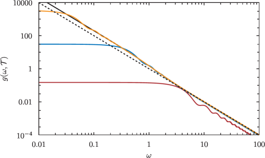
Figure 2: Scaled power spectrum $g(\omega,{\cal T})=\mu_{x}(f,T)/(v^{2}\tau_{R}^{3})$, Eq. (19), as function of the dimensionless frequency $\omega=\tau_{R}f$ for three values of the scaled observation time ${\cal T}=T/\tau_{R}$: ${\cal T}=1$ (red), ${\cal T}=10$ (blue) and ${\cal T}=100$ (orange). Solid (black) curve depicts the result in Eq.(15) (${\cal T}=\infty$). As a guide for an eye, the dashed line is the function $1/\omega^{2}$.

Further on, let us assume that $f$ is strictly positive and analyse how the infinite-$T$ form of Eq. (15) is approached when the observation time $T$ increases. To this end, we first note that $\mu_{x}(f,T)$ can be represented as

$$\mu_{x}(f,T)=v^{2}\tau_{R}^{3}\,g(\omega,{\cal T})\,,$$ (19)

where $\omega=\tau_{R}f$ is a dimensionless frequency and ${\cal T}=T/\tau_{R}$, as above, is a dimensionless observation time. $g(\omega,{\cal T})$ is then a scaled power spectral density. It can be computed explicitly but we omit here its lengthy expressions. In Fig. 2 we plot $g(\omega,{\cal T})$ for three values of ${\cal T}$, together with the limiting form in Eq. (15). We observe that, as a function of $\omega$, $g(\omega,{\cal T})$ generically shows a plateau at sufficiently small values of $\omega$, followed rather abruptly by a power-law decay $g(\omega,{\cal T})\sim 1/\omega^{2}$ at larger $\omega$. As ${\cal T}$ increases, the plateau appears at smaller values of $\omega$ and is shifted towards larger values. Even for a rather small value ${\cal T}=1$, the power-law decay of $g(\omega,{\cal T})$ appears very close to the ultimate infinite-${\cal T}$ form (15) (black solid line in Fig. 2), with a somewhat smaller amplitude. For larger observation times, (${\cal T}=10$ and ${\cal T}=100$), the agreement is nearly perfect and starts from smaller values of the scaled frequency. Unsurprisingly, the smaller $f$ is, the larger the observation time needs to be to approach the asymptotic result.

Lastly, we evaluate the total power as a function of the observation time. After straightforward calculations, we find

$$\int_{0}^{\infty}\textrm{d}f\,\mu_{x}(f,T) =\pi\frac{v^{2}\tau_{R}T}{2}\biggl{[}1-\frac{3}{2{\cal T}}+\frac{33}{24{\cal T}^{2}}-\frac{4}{3{\cal T}^{2}}e^{-{\cal T}}-\frac{1}{24{\cal T}^{2}}e^{-4{\cal T}}\biggr{]}\,,$$ (20)

$$\int_{0}^{\infty}\textrm{d}f\,\mu_{y}(f,T) =\pi\frac{v^{2}\tau_{R}T}{2}\biggl{[}1-\frac{5}{2{\cal T}}+\frac{63}{24{\cal T}^{2}}-\frac{8}{3{\cal T}^{2}}e^{-{\cal T}}+\frac{1}{24{\cal T}^{2}}e^{-4{\cal T}}\biggr{]}\,,$$

which shows that the total power diverges linearly with $T$ in the limit $T\to\infty$. We note that, in general, in order for the functional $S_{x}(f,T)$ in Eq.(4) to be meaningfully interpreted as the power spectral density of a non-stationary process $x(t)$, it has to verify some conditions. In particular, in the asymptotic limit $T\to\infty$, the total power as defined in the first line in Eqs.(20) must be equal, up to a factor $\pi$, to $\langle x^{2}(T)\rangle$ [51]. We observe that such a condition indeed holds.

3 Coefficient of variation and cross correlations

We now go beyond the standard spectral analysis to focus on two quantities that measure the level of fluctuations between realisations of the STSD $S_{x}(f,T)$ and $S_{y}(f,T)$. The first one is the coefficient of variation defined in Eq.(7) that quantifies the relative amplitude of fluctuations in either $S_{x}(f,T)$ or $S_{y}(f,T)$. The second is the Pearson coefficient $\rho_{S}$ that quantifies how correlated the values of $S_{x}(f,T)$ and $S_{y}(f,T)$ are. It is defined as

$$\rho_{S}=\dfrac{\left\langle S_{x}(f,T)S_{y}(f,T)\right\rangle-\mu_{x}(f,T)\mu_{y}(f,T)}{\sqrt{\left[\left\langle S^{2}_{x}(f,T)\right\rangle-\mu^{2}_{x}(f,T)\right]\left[\left\langle S^{2}_{y}(f,T)\right\rangle-\mu^{2}_{y}(f,T)\right]}}\,.$$ (21)

To this end, we need to calculate the second moments of $S_{x}(f,T)$ and $S_{y}(f,T)$, and the cross moment $\left\langle S_{x}(f,T)S_{y}(f,T)\right\rangle$. Once again, this can be done explicitly. The calculation itself is tedious but rather straightforward so that we skip the details and present the final results only.

3.1 Infinite-$T$ limit.

In the limit of an infinitely large observation time, the second moments obey

$$\left\langle S^{2}_{x}(f,\infty)\right\rangle=\left\langle S^{2}_{y}(f,\infty)\right\rangle=\tau_{R}^{2}v^{4}\,\frac{\left(9+10\tau_{R}^{2}f^{2}+3\tau_{R}^{4}f^{4}\right)}{f^{4}(1+\tau_{R}^{2}f^{2})^{2}}\,,$$ (22)

which yields the following compact result for the coefficient of variation :

$$\gamma(f,T=\infty)=\frac{\sqrt{5+6\tau_{R}^{2}f^{2}+2\tau_{R}^{4}f^{4}}}{2+\tau_{R}^{2}f^{2}}\,,\quad\left[\gamma^{(BM)}(f,T=\infty)=\frac{\sqrt{5}}{2}\,\,\,\text{for any $f>0$}\right]\,,$$ (23)

where the expression in the brackets is the same quantity computed for a standard BM (see, Ref. [58] for more details). We depict $\gamma$ as expressed in Eq.(23) in Fig. 3 as a function of the dimensionless frequency $\omega=\tau_{R}f$.

A few remarks are in order:

1. While $\gamma$ for standard BM is a constant independent of $f$ ($=\sqrt{5}/2$ for any $f>0$), for an ABP it is a monotonically increasing function of the frequency, when $T$ is infinitely large. It interpolates between $\sqrt{5}/2$, reached as expected in the limit $f\to 0$, and $\sqrt{2}$ achieved in the asymptotic limit $f\to\infty$. Hence, for any $f>0$ we have $\gamma(f,T=\infty)>\gamma^{(BM)}(f,T=\infty)$, which highlights the difference between the two random processes.

2. $S_{x}(f,\infty)$ and $S_{y}(f,\infty)$ are strongly fluctuating. Indeed, since $\gamma(f,\infty)>1$, the standard deviation of, say $S_{x}(f,\infty)$, is bigger than its mean value, $\mu_{x}(f,\infty)$, which implies that the latter is not representative of the actual behaviour.

3. The maximal value of $\gamma(f,\infty)$ is the same ($=\sqrt{2}$) as the one achieved in the limit $f\to\infty$ by the coefficient of variation of super-diffusive Gaussian processes (e.g. super-diffusive fractional BM [59] or super-diffusive scaled BM [60]). Such a coincidence is somewhat surprising, given the non-Gaussian nature of an ABP.

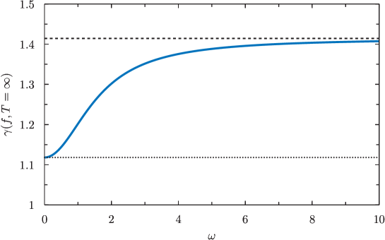
Figure 3: The coefficient of variation $\gamma$ for infinite observation time Eq.(23) as function of $\omega=\tau_{R}f$. The dashed line indicates the asymptotic value $\sqrt{2}$, achieved in the limit $f\to\infty$, while the dotted line corresponds to $\sqrt{5}/2$, the value of the coefficient of variation for a standard BM at any frequency.

3.2 Finite-$T$ behaviour of the coefficient of variation

Let us now consider the case of a finite observation time $T$, a more realistic situation if one is to compare with experiments or numerical simulations. In Fig. 4 we depict $\gamma(f,T)$ as function of the dimensionless frequency $\omega=\tau_{R}f$ for several values of the dimensionless observation time ${\cal T}=T/\tau_{R}$, together with the infinite-${\cal T}$ limit of Eq. (23) (solid black curve).

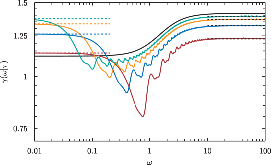
Figure 4: The coefficient of variation $\gamma(f,T)$ for finite $T$ as function of $\omega=\tau_{R}f$ for four values of the reduced observation time: ${\cal T}=10$ (red), ${\cal T}=20$ (blue), ${\cal T}=40$ (orange), and ${\cal T}=80$ (green). The solid (black) curve is the asymptotic form Eq. (23), which corresponds to ${\cal T}=\infty$. The horizontal dashed lines are the asymptotic results in Eqs. (24) and (25).

We observe, interestingly enough, the non-commutation of limits $T\to\infty$ and $f\to 0$ that we have mentioned previously so that one obtains a completely different behaviour for $\gamma$ depending on which of the limits is taken first. More precisely, the small-$f$ behaviour of $\gamma$ at finite $T$ does not approach $\gamma(f,T=\infty)$ as $T$ is increased. The latter approaches a constant value $\sqrt{5}/2$ as $f\to 0$ while the former tends to some $T$-dependent value which drifts away from $\sqrt{5}/2$ as $T$ increases. This is again very different from the behaviour of $\gamma^{(BM)}(f=0,T)$ for standard BM which also shows the non-commutativity of limits but equals $\sqrt{2}$ for any $T$ when $f=0$ [58].

The $T$-dependent expression $\gamma(f=0,T)$ is rather cumbersome. However, in the limit $T\to\infty$ it reduces to the following asymptotic expansion

$$\gamma(f=0,T) =\sqrt{2}-\frac{189}{40\sqrt{2}\,{\cal T}}+\frac{57369}{6400\sqrt{2}\,{\cal T}^{2}}+O\left(\frac{1}{{\cal T}^{3}}\right)\,.$$ (24)

Therefore, $\gamma(f=0,T)$ attains the limiting value $\sqrt{2}$ of standard BM but only in the limit $T\to\infty$ (whereas $\gamma^{(BM)}(f=0,T)=\sqrt{2}$ for any $T$). In the opposite limit $f\to\infty$, $\gamma(f,T)$ approaches a limiting $T$-dependent value, which is different from $\sqrt{2}$ attained at $T\to\infty$. For large $T$, the asymptote becomes

$$\gamma(f=\infty,T) =\sqrt{2}-\frac{21}{8\sqrt{2}\,{\cal T}}+\frac{55}{768\sqrt{2}\,{\cal T}^{2}}+O\left(\frac{1}{{\cal T}^{3}}\right)\,.$$ (25)

One thus finds that, this time, the limits commute and one does recover in the limit $T\to\infty$ the coefficient of variation $\gamma(f=\infty,T=\infty)$ computed in Eq. (23). The limits $f\to\infty$ and $T\to\infty$ can thus be taken in either order.

Further on, we present in Fig. 5 a more detailed comparison between the coefficients of variation for an ABP and a standard BM. We recall that the latter is function of the product $fT$ only [58] and hence, we plot $\gamma(f,T)$ and $\gamma^{(BM)}(f,T)$ as functions of $fT$. Since in the active case $\gamma$ depends also on $\tau_{R}$, we plot $\gamma(f,T)$ for four different values of the dimensionless observation time ${\cal T}=T/\tau_{R}$. We observe that at small $fT$, $\gamma(f,T)$ differs from its BM counterpart and attains a non-universal $\tau_{R}$-dependent value when $fT\to 0$. In this region, $\gamma(f,T)$ is smaller than $\gamma^{(BM)}(f,T)$ and the difference becomes more pronounced the smaller ${\cal T}$ is. After a minimum observed at some intermediate value of $fT$, which is only weakly dependent on ${\cal T}$ (while the minimum itself gets progressively deeper the larger ${\cal T}$ is), we observe a change in the behaviour at large $fT$ such that $\gamma(f,T)$ becomes larger than $\gamma^{(BM)}(f,T)$. There, as $fT\to\infty$, $\gamma(f,T)$ tends to a constant $\tau_{R}$-dependent value which exceeds $\sqrt{5}/2$, the limiting value reached by $\gamma^{(BM)}(f,T)$ [58]. Most strikingly, when ${\cal T}$ increases $\gamma(f,T)\to\sqrt{2}$, away from the standard BM result. Overall, Fig. 5 reveals pronounced differences between these two paradigmatic random processes. Although they both have a similar long-time behaviour if one looks at the mean-squared displacement only, the coefficient of variation $\gamma$ is one measurement that allows to distinguish between the two.

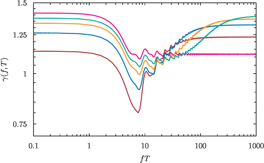
Figure 5: The coefficients of variation $\gamma(f,T)$ and $\gamma^{(BM)}(f,T)$ (magenta) as functions of $fT$. The results for an ABP are presented for ${\cal T}=T/\tau_{R}=80$ (green), ${\cal T}=40$ (orange), ${\cal T}=20$ (blue) and ${\cal T}=10$ (red).

3.3 Pearson correlation coefficient

Figure 6: Pearson correlation coefficient $\rho_{S}$ as function of $fT$ for ${\cal T}=T/\tau_{R}=10$ (red), $20$ (blue), $30$ (orange), and $40$ (green).

The evolution of both components of the ABP position (see Eqs. (1)) originates from the same random process $\theta(t)$ and are thus clearly coupled, which is also obvious from the requirement that the module of the velocity Eq. (3) be fixed. Clearly, this implies that $S_{x}(f,T)$ and $S_{y}(f,T)$ are statistically correlated. Below, we study the extent of such correlations by analysing the Pearson coefficient defined in Eq. (21). The behaviour of this coefficient as a function of $fT$ is depicted in Fig. 6 for four values of the dimensionless observation time ${\cal T}=T/\tau_{R}$. Physically, such a representation means that we fix the observation time $T$ and trace the $f$-dependence of $\rho_{S}$ for four different values of $\tau_{R}$ (going from green to red when increasing $\tau_{R}$).

We observe first that $S_{x}(f,T)$ and $S_{y}(f,T)$ are always positively correlated since the Pearson coefficient is always positive. Second, we see that $\rho_{S}$ is a decreasing function of the persistence time $\tau_{R}$. Such a behaviour seems rather counter-intuitive at first glance since decreasing $\tau_{R}$ is akin to increasing noise, thus bringing an ABP closer to standard BM. One could then expect a decorrelation of the components as $\tau_{R}$ is reduced. On the other hand, the correlations between $x$ and $y$ appear precisely because of the noise. In the extreme limit $\tau_{R}\to\infty$ the trajectories do not fluctuate, neither do the STSD and $\rho_{s}$ thus vanishes. This gives an argument as to why the Pearson coefficient increases when $\tau_{R}$ decreases. Even stronger, our analytical analysis (not shown here) indicates that $\rho_{s}$ reaches its maximal value $=1$ in the limit $T/\tau_{R}\rightarrow\infty$. The STSD of $x$ and $y$ are then perfectly correlated.

4 Effects of a translational diffusion

In writing the dynamics of an ABP Eq. (1), we have assumed that it moves in a solvent imposing a high friction such that it reaches a terminal velocity $v$. In principle, the solvent also imparts translational noise on the particle. Although the diffusion coefficient $D$ originating from such a standard mechanism of Brownian motion is typically much smaller than the effective diffusion $D_{e}$ due to self-propulsion [13], the presence of a translational diffusion may affect the functional form of the spectral density of trajectories. In this Section, we investigate how some of the results derived above, especially concerning the power spectral density and the coefficient of variation, are modified in presence of translational noise.

We generalise the model of Eqs. (1) in a standard way by adding to their right-hand-side independent uncorrelated Gaussian white-noises so that the trajectories $x_{\rm D}(t)$ and $y_{\rm D}(t)$ read

$$x_{\rm D}(t) =X_{t}+v\int_{0}^{t}\textrm{d}\tau\,\cos\theta(\tau)\,,\quad x_{\rm D}(0)=0\,,$$ (26)

$$y_{\rm D}(t) =Y_{t}+v\int_{0}^{t}\textrm{d}\tau\,\sin\theta(\tau)\,,\quad y_{\rm D}(0)=0\,,$$

where $X(t)$ and $Y(t)$ denote independent Brownian motions starting at the origin at $t=0$, which obey $\overline{X_{t}}=\overline{Y_{t}}=0$ and $\overline{X_{t}X_{t^{\prime}}}=\overline{Y_{t}Y_{t^{\prime}}}=2D\,{\rm min}\left(t,t^{\prime}\right)$, and the overbar denotes averaging over these additional Gaussian noises.

Adding translational noise, the mean-squared displacement for, say, the $x$-component becomes

$$\overline{\langle x_{\rm D}^{2}(t)\rangle}=2Dt+v^{2}\tau_{R}^{2}\biggl{[}\tau-\frac{3}{4}+\frac{2}{3}e^{-\tau}+\frac{1}{12}e^{-4\tau}\biggr{]}\,,\quad\tau=t/\tau_{R}\,.$$ (27)

The second term in this expression is identical to our previous result Eq. (13). The translational noise thus appears as a purely additive contribution. In the limit $t\to\infty$, one finds from Eq. (27) a standard Brownian behaviour of the form $\overline{\langle x_{\rm D}^{2}(t)\rangle}\simeq 2D_{tot}t$ with $D_{tot}=D_{e}+D$. An analogous result for the $y$-component is obtained by merely replacing the second term in Eq. (27) by the appropriate expression from Eq. (13). As a consequence, the power spectral densities for an infinitely long observation time $\mu^{\rm D}_{x}(f)$ and $\mu^{\rm D}_{y}(f)$ of the processes $x_{\rm D}(t)$ and $y_{\rm D}(t)$, respectively, after averaging over the additional white noises, are given by

$$\mu^{\rm D}_{x}(f,D)=\mu^{\rm D}_{y}(f,D)=\frac{2D_{e}+4D}{f^{2}}+\frac{2D_{e}}{f^{2}}\frac{1}{1+\tau_{R}^{2}f^{2}}\,.$$ (28)

Therefore, here again the translational diffusion enters additively with a contribution corresponding to standard BM with diffusion constant $D$.

Next, we consider how translational diffusion affects the coefficient of variation. To this end, let us first note that since the translational and rotational noises are uncorrelated, the variance ${\rm var}\left(S^{\rm D}_{x}(f,T,D)\right)$ of the process $x_{\rm D}(t)$ naturally decomposes into the variance of the process $x(t)$, which we have studied in the previous Sections, and the variance of the spectral density of a Brownian motion $X_{t}$, i.e.

$${\rm var}\left(S^{\rm D}_{x}(f,T,D)\right) ={\rm var}\left(S_{x}(f,T)\right)+{\rm var}\left(S_{X}(f,T,D)\right)$$

$$=\left\langle S^{2}_{x}(f,T)\right\rangle-\left\langle S_{x}(f,T)\right\rangle^{2}+\overline{S^{2}_{X}(f,T,D)}-\overline{S_{X}(f,T,D)}^{2}\,.$$ (29)

The second moment of the spectral density of individual trajectories $x(t)$ has been calculated in Sec. 3 (see Eq. (22) for its explicit form in the limit $T\to\infty$). The variance of the spectral density of individual trajectories of a standard Brownian motion $X_{t}$ can be found in an explicit form in Ref. [58] for arbitrary $T$ and $f$. Capitalising on these results, we define the coefficient $\Gamma(f,T,D)$ of the process $x_{\rm D}(t)$:

$$\Gamma(f,T,D)=\dfrac{\sqrt{{\rm var}\left(S^{\rm D}_{x}(f,T,D)\right)}}{\mu^{\rm D}_{x}(f,T,D)}\,.$$ (30)

Formally, $\Gamma(f,T,D)$ depends on $f$, $T$, $D$, $\tau_{R}$ and $v$. However, since $\Gamma$ is dimensionless, it must depend only on dimensionless combinations of these parameters. A straightforward scaling analysis shows that, indeed, $\Gamma(f,T,D)$ is a function of only ${\cal T}=T/\tau_{R}$, the product $fT$ and the dimensionless parameter

$$\alpha=\frac{v^{2}T}{D}\,.$$ (31)

The latter interpolates between two limits: $\alpha=0$ corresponding to a standard Brownian motion without any self-propulsion, in which case $\Gamma(f,T,D)$ reduces to the expression obtained in Ref. [58], and $\alpha=\infty$ – the case studied in the previous Sections, i.e. an active Brownian motion without a translational diffusion. The coefficient of variation $\Gamma(fT,\alpha,{\cal T})$ is plotted in Fig. 7 for several values of the parameter $\alpha$ as function of $fT$ including the two limiting cases of passive BM ($\alpha=0$) and ABP ($\alpha=\infty$). They exhibit somewhat different trends. For passive BM, $\gamma$ decreases (with superimposed small oscillations) when $fT$ increases from the value $\sqrt{2}$ to a smaller value $\sqrt{5}/2$. On the contrary, for the purely active motion, the coefficient of variation first decreases from $\sqrt{2}$ to a minimal value before rising again to the limiting value $\sqrt{2}$ in virtue of Eq. (25). As a consequence, upon a variation of the value of $\alpha$, we observe a change of the trend in the behaviour of $\Gamma(fT,\alpha,{\cal T})$ which appears to be rather non-trivial due to an interplay between rotational and translational diffusion.

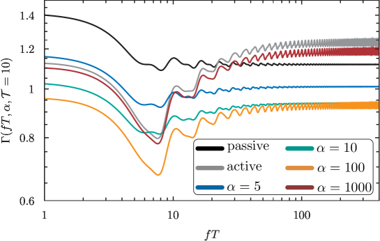
Figure 7: The coefficient $\Gamma(fT,\alpha,{\cal T})$ of variation in presence of translation diffusion as function of $fT$ for ${\cal T}=10$ and several values of the parameter $\alpha$ defined in Eq. (31). The passive case corresponds to $\alpha=0$ and the purely active case is reached when $\alpha\to\infty$.

More specifically, scaling analysis shows that $\Gamma(fT,\alpha,{\cal T})$ exhibits in the limit $\alpha\to\infty$ a behaviour of the form

$$\Gamma(fT,\alpha,{\cal T})=\gamma(f,T)\left(1-\frac{\beta(f,T)}{\alpha}+O\left(\frac{1}{\alpha^{2}}\right)\right)\,,$$ (32)

where $\gamma(f,T)$ is the coefficient of variation for an active Brownian motion and $\beta(f,T)$ is a computable function. Indeed, we see that for $\alpha=1000$ (see the magenta curve in Fig. 7) $\Gamma(fT,\alpha=1000,{\cal T})$ is only slightly shifted downwards with respect to the limiting curve $\Gamma(fT,\alpha=\infty,{\cal T})$. We remark that this case is the most relevant experimentally since we expect in practice the diffusion coefficient $D_{e}$ due to rotational motion and self-propulsion to be much bigger than the coefficient $D$ of translational diffusion. For $\alpha=100$, we have that $\Gamma(fT,\alpha,{\cal T})$ is still shifted downwards for any value of the parameter $fT$. However, upon a further decrease of $\alpha$ the opposite trend establishes – the curve $\Gamma(fT,\alpha,{\cal T})$ starts to move upwards (see the curves corresponding to $\alpha=10$ and $\alpha=5$ in Fig. 7) and ultimately approaches the black curve describing the behaviour in the purely Brownian case.

5 Conclusions

We analysed the spectral properties of individual trajectories of an active Brownian motion, as exemplified by the dynamics of a chemically-active Janus colloid confined to move on a fluid-fluid interface.

We evaluated the standardly defined power spectral density, which is an ensemble-averaged property taken in the limit of an infinite observation time $T$. The resulting expression Eq.(15) has a more complicated form than the power spectral density of a standard Brownian motion (passive case): in addition to a simple power law dependence on the frequency $f$, as established for a standard Brownian motion, Eq. (15) contains the Lorentzian function specific to dynamics in presence of a constant restoring force. This causes a departure from the standard Brownian behaviour for the intermediate values of $f$, while the large-$f$ and the small-$f$ asymptotic behaviours appear to be essentially the same. More pronounced differences between the active and the passive case are observed for finite observation times – the more realistic situation in experimental and numerical analyses. We have demonstrated that for finite $T$ the ensemble-averaged spectral density is characterised by a plateau-like region in the short-$f$ limit, which extends over several orders of magnitude of $f$ and is absent for the passive counterpart.

Going beyond the standard approach, we concentrated on fluctuations around the ensemble-averaged spectral density and determined the coefficient of variation of the distribution of a single-trajectory power spectral density. For this property, our analysis revealed substantial differences between active and passive Brownian motion. Here, the difference is striking not only for finite but also infinitely large $T$. On this basis, we discussed the similarities and the distinctive features showing that the spectral content of trajectories provides important information and allows to distinguish between the two processes.

Finally, we addressed as well the effect of translational diffusion on the power spectral density and the coefficient of variation of an active Brownian motion. We have shown that in the limit of small translational diffusion (compared to the diffusion induced by self-propulsion) no singular non-analytic behaviour emerges so that the translational diffusion only induced small quantitative changes. For larger values of $D$, however, interesting non-monotonic behaviours take place.

Our result constitutes a first step in analysing the spectral properties of the trajectories of active particles. Going further in that direction, it will be important to determine the spectral content of other types of active particles, in particular the other experimentally relevant class of run-and-tumble particles.

References

References

- [1] M. Ballerini et al., Interaction ruling animal collective behavior depends on topological rather than metric distance: Evidence from a field study, Proc. Natl. Acad. Sci. USA 105, 1232 (2008).
- [2] Y. Katz, K. Tunstrom, C. C. Ioannou, C. Huepe, and I. D. Couzin, Collective States, Multistability and Transitional Behavior in Schooling Fish, Proc. Natl. Acad. Sci. USA 108, 18720 (2011).
- [3] H. C. Berg, E. Coli Motion (Heidelberg: Springer, 2004)
- [4] W. F. Paxton, S. Sundararajan, T. E. Mallouk, and A. Sen, Chemical locomotion, Angew. Chem. Int. Ed. 45, 5420 (2006).
- [5] J. R. Howse, R. A. Jones, A. J. Ryan, T. Gough, R. Vafabakhsh, and R. Golestanian, Self-Motile Colloidal Particles: From Directed Propulsion to Random Walk, Physical Review Letters 99, 048102 (2007).
- [6] H. Chaté and B. Mahault, Dry Aligning Dilute Active Matter: A Synthetic and Self-Contained Overview, ArXiv Preprint ArXiv:1906.05542 (2019).
- [7] M. E. Cates and J. Tailleur, Motility-Induced Phase Separation, Annu. Rev. Condens. Matter Phys. 6, 219 (2015).
- [8] C. Dombrowski, L. Cisneros, S. Chatkaew, R. E. Goldstein, and J. O. Kessler, Self-Concentration and Large-Scale Coherence in Bacterial Dynamics, Physical Review Letters 93, 098103 (2004).
- [9] C. Bechinger et al., Active particles in complex and crowded environments, Rev. Mod. Phys. 88, 045006 (2016).
- [10] G. Gompper et al., The motile active matter roadmap, J. Phys. Condens. Matter 32, 193001 (2020).
- [11] G. Szamel, Self-Propelled Particle in an External Potential: Existence of an Effective Temperature, Physical Review E 90, 012111 (2014).
- [12] É. Fodor, C. Nardini, M. E. Cates, J. Tailleur, P. Visco, and F. van Wijland, How Far from Equilibrium Is Active Matter?, Phys. Rev. Lett. 117, 038103 (2016).
- [13] F. Ginot, A. Solon, Y. Kafri, C. Ybert, J. Tailleur, and C. Cottin-Bizonne, Sedimentation of Self-Propelled Janus Colloids: Polarization and Pressure, New Journal of Physics 20, 115001 (2018).
- [14] E. Lauga, W. R. DiLuzio, G. M. Whitesides, and H. A. Stone, Swimming in Circles: Motion of Bacteria near Solid Boundaries, Biophysical Journal 90, 400 (2006).
- [15] P. Bayati, M. N. Popescu, W. E. Uspal, S. Dietrich, and A. Najafi, Dynamics near planar walls for various model self-phoretic particles, Soft Matter 15, 5644 (2019).
- [16] A. P. Solon et al., Pressure is not a state function for generic active fluids, Nature Phys. 11, 673 (2015).
- [17] A. P. Solon, M. E. Cates, and J. Tailleur, Active brownian particles and run-and-tumble particles: A comparative study, Eur. Phys. J. Spec. Top. 224, 1231 (2015).
- [18] M. J. Schnitzer, Theory of Continuum Random Walks and Application to Chemotaxis, Physical Review E 48, 2553 (1993).
- [19] Y. Fily and M. C. Marchetti, Athermal Phase Separation of Self-Propelled Particles with No Alignment, Phys. Rev. Lett. 108, 235702 (2012).
- [20] J. Palacci, C. Cottin-Bizonne, C. Ybert, and L. Bocquet, Sedimentation and Effective Temperature of Active Colloidal Suspensions, Physical Review Letters 105, 088304 (2010).
- [21] I. Buttinoni, G. Volpe, F. Kümmel, G. Volpe, and C. Bechinger, Active Brownian Motion Tunable by Light, Journal of Physics: Condensed Matter 24, 284129 (2012).
- [22] S. Ebbens, M. H. Tu, J. R. Howse, and R. Golestanian, Size dependence of the propulsion velocity for catalytic Janus-sphere swimmers, Phys. Rev. E 85, 020401 (2012).
- [23] G. Oshanin, M. N. Popescu, and S. Dietrich, Active colloids in the context of chemical kinetics, J. Phys. A: Math. Theor. 50, 134001 (2017).
- [24] L. Angelani, R. Di Leonardo, and M. Paoluzzi, First-passage time of run-and-tumble particles, The European Physical Journal E 37, 59 (2014)
- [25] F. Detcheverry, Generalized run-and-turn motions: From bacteria to Lévy walks, Phys. Rev. E 96, 012415 (2017).
- [26] K. Malakar et al, Steady state, relaxation and first-passage properties of a run-and-tumble particle in one-dimension, JSTAT 043215 (2018).
- [27] T. Bertrand, Y. Zhao, O. Bénichou, J. Tailleur, and R. Voituriez, Optimized Diffusion of Run-and-Tumble Particles in Crowded Environments, Phys. Rev. Lett. 120, 198103 (2018).
- [28] A. Dhar, A. Kundu, S. N. Majumdar, S. Sabhapandit, and G. Schehr, Run-and-tumble particle in one-dimensional confining potentials: Steady-state, relaxation, and first-passage properties, Phys. Rev. E 99, 032132 (2019).
- [29] I. Santra, U. Basu, and S. Sabhapandit, Run-and-tumble particles in two dimensions: Marginal position distributions, Phys. Rev. E 101, 062120 (2020).
- [30] F. Mori, P. L. Doussal, S. N. Majumdar, and G. Schehr, Universal Survival Probability for a d-Dimensional Run-and-Tumble Particle, Phys. Rev. Lett. 124, 090603 (2020).
- [31] I. Santra, U. Basu, and S. Sabhapandit, Run-and-tumble particles in two dimensions under stochastic resetting conditions, J. Stat. Mech. 113206 (2020); https://iopscience.iop.org/article/10.1088/1742-5468/abc7b7
- [32] P. Singh and A. Kundu, Local time for run and tumble particle, Phys. Rev. E 103, 042119 (2021).
- [33] C. Reichhardt and C. J. O. Reichhardt, Clogging, dynamics, and reentrant fluid for active matter on periodic substrates, Phys. Rev. E 103, 062603 (2021).
- [34] C. Kurzthaler, S. Leitmann, and T. Franosch, Intermediate scattering function of an anisotropic active Brownian particle, Scientific Reports 6, 36702 (2016).
- [35] A. Pototsky and H. Stark, Active Brownian particles in two-dimensional traps, EPL 98, 50004 (2012).
- [36] F. J. Sevilla and L. A. G. Nava, Theory of diffusion of active particles that move at constant speed in two dimensions, Phys. Rev. E 90, 022130 (2014).
- [37] U. Basu, S. N. Majumdar, A. Rosso, and G. Schehr, Active Brownian motion in two dimensions, Phys. Rev. E 98, 062121 (2018).
- [38] S. N. Majumdar and B. Meerson, Toward the full short-time statistics of an active Brownian particle on the plane, Phys. Rev. E 102, 022113 (2020).
- [39] I. Santra, U. Basu, and S. Sabhapandit, Active Brownian Motion with Directional Reversals, Phys. Rev. E 104, L012601 (2021).
- [40] P. Romanczuk, M. Bär, W. Ebeling, B. Lindner, and L. Schimansky-Geier, Active Brownian particles. Eur. Phys. J. Special Topics 202, 1 (2012).
- [41] D. Martin, J. O’Byrne, M. E. Cates, E. Fodor, C. Nardini, J. Tailleur, and F. van Wijland, Statistical Mechanics of Active Ornstein-Uhlenbeck Particles, Physical Review E 103, 032607 (2021).
- [42] P. Kalinay, Reduced dynamics of a one-dimensional Janus particle, Phys. Rev. E 104, 014608 (2021).
- [43] P. Malgaretti, M. N. Popescu, and S. Dietrich, Active colloids at fluid interfaces, Soft Matter 12, 4007 (2016).
- [44] W. Fei, Y. Gu, and K. J. M. Bishop, Active colloidal particles at fluid-fluid interfaces, Curr. Opin. Colloid Interface Sci. 32, 57 (2017).
- [45] D. Mumford, Elastica and Computer Vision, in Algebraic Geometry and Its Applications (Springer, 1994), p. 491
- [46] R. Grossmann, F. Peruani, and M. Bär, Diffusion properties of active particles with directional reversal, New J. Phys. 18, 043009 (2016).
- [47] M. E. Cates and J. Tailleur, When Are Active Brownian Particles and Run-and-Tumble Particles Equivalent? Consequences for Motility-Induced Phase Separation, EPL (Europhysics Letters) 101, 20010 (2013).
- [48] P. Flandrin, On the spectrum of fractional Brownian motions, IEEE Trans. Inf. Theory 35, 197 (1989).
- [49] N. Niemann, H. Kantz, and E. Barkai, Fluctuations of Noise and the Low-Frequency Cutoff Paradox, Phys. Rev. Lett. 110, 140603 (2013).
- [50] N. Leibovitch and E. Barkai, Aging Wiener-Khinchin Theorem, Phys. Rev. Lett. 115, 080602 (2015).
- [51] N. Leibovich, A. Dechant, E. Lutz, and E. Barkai, Aging Wiener-Khinchin theorem and critical exponents of noise, Phys. Rev. E 94, 052130 (2016).
- [52] O. Bénichou, P. L. Krapivsky, C. Mejía-Monasterio, and G. Oshanin, Temporal correlations of the running maximum of a Brownian trajectory, Phys. Rev. Lett. 117, 080601 (2016).
- [53] D. S. Dean, A. Iorio, E. Marinari, and G. Oshanin, Sample-to-sample fluctuations of power spectrum of a random motion in a periodic Sinai model, Phys. Rev E 94, 032131 (2016).
- [54] K. Berg-Sørensen and H. Flyvbjerg, Power spectrum analysis for optical tweezers, Rev. Sci. Instrum. 75, 594 (2004).
- [55] S. N. Majumdar and G. Oshanin, Spectral content of fractional Brownian motion with stochastic reset, J. Phys. A: Math. Theor. 51, 435001 (2018).
- [56] A. Squarcini, E. Marinari, and G. Oshanin, Passive advection of fractional Brownian motion by random layered flows, New J. Phys. 22, 053052 (2020).
- [57] Z. R. Fox, E. Barkai, and D. Krapf, Aging power spectrum of membrane protein transport and other subordinated random walks; DOI:10.21203/rs.3.rs-286804/v1
- [58] D. Krapf et al., Power spectral density of a single Brownian trajectory: what one can and cannot learn from it, New J. Phys. 20, 023029 (2018).
- [59] D Krapf et al., Spectral content of a single non-Brownian trajectory, Phys. Rev. X 9, 011019 (2019).
- [60] V. Sposini, R. Metzler, and G. Oshanin, Single-trajectory spectral analysis of scaled Brownian motion, New J. Phys. 21, 073043 (2019).
- [61] V. Sposini, D. S. Grebenkov, R. Metzler, G. Oshanin, and F. Seno, Universal spectral features of different classes of random-diffusivity processes, New J. Phys. 22, 063056 (2020).
- [62] C. Mejía-Monasterio, S. Nechaev, G. Oshanin, and O. Vasilyev, Tracer diffusion on a crowded random Manhattan lattice, New J. Phys. 22, 033024 (2020).
- [63] S. Cerasoli, S. Ciliberto, E. Marinari, G. Oshanin, L. Peliti, and L. Rondoni, Spectral fingerprints of non-equilibrium dynamics: the case of a Brownian gyrator, in preparation
- [64] C. W. Gardiner, Handbook of stochastic methods (Vol. 3, pp. 2-20). Berlin: springer. (1985)
- [65] F. Den Hollander, S. N. Majumdar, J. M. Meylahn, and H. Touchette, Properties of additive functionals of Brownian motion with resetting J. Phys. A: Math. Theor. 52, 175001 (2019).
- [66] B. Meerson, Large fluctuations of the area under a constrained Brownian excursion, J. Stat. Mech. 013210 (2019).
- [67] T. Agranov, P. Zilber, N. R. Smith, T. Admon, Y. Roichman, and B. Meerson, Airy distribution: Experiment, large deviations and additional statistics, Phys. Rev. Res. 2, 013174 (2020).
- [68] B. Meerson, Area fluctuations on a sub-interval of Brownian excursion, J. Stat. Mech. 103208 (2020).