Initialization for Nonnegative Matrix Factorization: a Comprehensive Review

Abstract

Non-negative matrix factorization (NMF) has become a popular method for representing meaningful data by extracting a non-negative basis feature from an observed non-negative data matrix. Some of the unique features of this method in identifying hidden data put this method amongst the powerful methods in the machine learning area. The NMF is a known non-convex optimization problem and the initial point has a significant effect on finding an efficient local solution. In this paper, we investigate the most popular initialization procedures proposed for NMF so far. We describe each method and present some of their advantages and disadvantages. Finally, some numerical results to illustrate the performance of each algorithm are presented.

Keywords Non-negative matrix factorization $\cdot$ Initialization algorithms

1 Introduction

Over the last few years, the low-rank approximation, which is approximating a matrix by one whose rank is less than that of the original matrix has been an important technique and highly popular method in data science. Low-rank approximations are fundamental and widely used tools for data analysis, dimensionality reduction, and data compression. This method appears in many applications such as, image processing (Friedland et al., 2011), text data-latent semantic indexing, text mining (Eldén, 2003; Skillicorn, 2007), and machine-learning (Murphy, 2012; Lee et al., 2013). Low-rank approximations find two matrices of the much lower-rank that approximate a high-dimensional matrix $X$ such that:

$$X_{m\times n}\approx W_{m\times r}H_{r\times n},$$ (1)

where

$${r}<<\min(m,n)$$ (2)

in which $r$ is so called rank of the matrix. There are very widespread matrix decompositions that give a low-rank approximation, for example we can refer to singular value decompositions (SVD) (Golub and Van Loan, 1996; Alter et al., 2000; Wall et al., 2003). It can provides the optimal rank and gives the appropriate of low-rank approximation of a matrix (Datta, 2010; Sundarapandian, 2008; Trefethen and Bau III, 1997). Unfortunately, these approximations usually do not actualize eligible structural constraints such as element-wise non-negativity (Recht et al., 2010; Paruolo, 2000; Miller and de Callafon, 2012; Chu et al., 2003). For this reason, other concepts based on convex optimization have been developed such as URV, SDD, PCA, ICA, CUR, QR, and NMF (Drineas et al., 2006; Smilde et al., 2005; Meyer, 2000; Kolda and O’leary, 1998; Esposito et al., 2021; Meng et al., 2016; Sompairac et al., 2019). Each of these approaches is based on different constraints that characterize the final properties of the matrix factors, leading to different optimization problems and numerical algorithms that must be used.

Non-negative Matrix Factorization (NMF) is an unsupervised data decomposition technique, akin to latent variable analysis, that can be used for feature learning, topics recovery, clustering, temporal segmentation, filtering, and source separation coding as with vector quantization. As a matter of fact, this method obtains parts-based, compression, and discriminant representation of the original data as well as enhancing the interpretability by using decomposes the main matrix into additive parts (Lee and Seung, 1999). There have been some significant developments (Aggarwal and Reddy, 2014) in using NMF for computation of the linear part-based representation of non-negative data. Therefore, NMF can be considered as a method in the machine learning area which enhances the interpretability of the results. Therefore, interpretability can be considered as one of the advantages of NMF. In addition, robustness is another property of NMF that can be applied to handle noise and estimates the missing values. Suppose that $X$ is a real and non-negative $m\times n$ matrix. NMF finds two real and non-negative matrices $W\in\mathbb{R}^{m\times r}$ and $H\in\mathbb{R}^{r\times n}$, such that:

$$X\approx WH.$$

There are various approaches to find matrices $W$ and $H$. An efficient way for this purpose is to apply optimization tools. To use optimization algorithms, we need a criterion for measuring the difference between the original matrix, that is, $X$, and the results, i.e, the matrix $WH$. This measure is called objective function and can be considered as a measure for denoting an error. Here, we review two of the most common measures:

• Frobinous norm-based algorithm (SED): In this case, we use the Euclidean distance between origin matrix $X$ and its approximation $WH$ as the similarity measure to derive the following objective function, which is based on the Frobenius norm for matrices:

  $$\min_{W,H}f(W,H)=\frac{1}{2}\|X-WH\|^{2}_{F},~{}~{}\text{such that}~{}W\geq 0~{}\text{and}~{}H\geq 0.$$ (3)

• Divergence-based algorithm (GKLD): This case is the most popular in real applications, the corresponding objective function that characterizes the similarity between matrix $X$ and matrix $WH$ (called divergence) and is given by (Lee and Seung, ):

  $$\min_{W,H\geq 0}KL(X;WH)=\sum_{i,j}(X_{ij}\log\frac{X_{ij}}{(WH)_{ij}}-X_{ij}+(WH)_{ij}).$$ (4)

Note that objective functions given by (3) and (4) are non-convex in both $W$ and $H$. So, iterative approaches suggested for solving them guarantee to converge to some local minimum (more precisely, stationary points), but require initialization mechanisms that can greatly affect their convergence rate. “Good" initial values for NMF are defined as follows (Boutsidis and Gallopoulos, 2008):

• One that leads to rapid error reduction and faster convergence.

• One that leads to better overall error at convergence.

There have been numerous results devoted to the initialization approaches for the NMF (Casalino et al., 2014; Esposito, 2021). So, it seems that a systematic survey is of necessity and consequence. This review paper will summarize the most existing initialization strategies for NMF. We first present some common methods for solving NMF problem and then focus on the initialization approaches for this problem. We collect the most common initialization algorithms and investigate the advantages and disadvantages of them. Finally, we perform Lee’s algorithm to compare the efficiency of the initialization methods. We perform the algorithm on the ORL dataset consisting of face images and compare the results.

The rest of this paper is organized as follows. Section 2 briefly reviews the NMF problem and presents some common approaches for solving it and classifies the existing initialization methods. In Section 3 we have a comprehensive review of random initialization seeding methods and present their algorithm. We preset various clustering initialization strategies in Section 4. Heuristic schemes for initialization are invested in Section5. In Section 6, we review some low-rank approximation methods. In Section 7 we present some numerical results of performing Lee’s Algorithm on the ORL database to demonstrate the performance of each initialization strategy. We finally end up the paper by giving some concluding remarks in Section 8.

2 NMF methods

In this section, we review some common approaches for solving NMF. We start this section with recall multiplicative update rules, i.e., the SED-MU and GKLD-MU proposed by Lee and Seung (Lee and Seung, ). These methods have still been widely used as the baseline. The SED-MU update the matrices $W$ and $H$ by using the following strategy:

$$W^{k+1}_{ia} = W^{k}_{ia}\frac{(X{H^{k}}^{T})_{ia}}{(W^{k}H^{k}{H^{k}}^{T})_{ia}},\qquad\forall i,a;$$ (5)

$$H^{k+1}_{bj} = H^{k}_{bj}\frac{({W^{k+1}}^{T}X)_{bj}}{({W^{k+1}}^{T}W^{k+1}H^{k})_{bj}},\qquad\forall b,j.$$ (6)

Moreover, the GKLD-MU can be formulated as:

$$W_{ia}\leftarrow W_{ia}\sum_{j}\frac{X_{ij}}{(WH)_{ij}}H_{aj},$$

$$W_{ia}\leftarrow\frac{W_{ia}}{\sum_{j}W_{ja}},\qquad~{}~{}\text{and}~{}\quad H_{aj}\leftarrow H_{aj}\sum_{i}W_{ia}\frac{X_{ij}}{(WH)_{ij}}.$$

It is proven that the multiplicative update rules converge to a local minimum (Lee and Seung, ).

Another popular approach for solving NMF applying SED as the objective function is called Alternating Non-negative Least Squares (ANLS), which is alternating least squares (ALS) modified under the non-negativity constraint. This approach finds two matrices $W$ and $H$ by solving the following optimization problems:

$$W^{k+1}=\arg\min_{W\geq 0}f(W,H^{K})=\frac{1}{2}\|X-WH^{k}\|_{F}^{2},$$ (7)

$$H^{k+1}=\arg\min_{H\geq 0}f(W^{k+1},H)=\frac{1}{2}\|X-W^{k+1}H\|_{F}^{2}.$$ (8)

Although the original problem (3) is non-convex and NP-hard with respect to variables $W$ and $H$, the sub-problems (7) and (8) are convex problems. However, these subproblems may have multiple optimal solutions because they are not strictly convex (Gong and Zhang, 2012).

To accelerate the convergence rate, one popular method is to apply gradient descent algorithms with additive update rules. Other techniques such as conjugate gradient, projected gradient, interior point method, and more sophisticated second-order schemes like Newton and Quasi-Newton methods are also in consideration (Bonettini et al., 2008; Guan et al., 2012; Gong and Zhang, 2012; Huang et al., 2015; Fathi-Hafshejani and Moaberfard, 2020). To satisfy the non-negativity constraint, the updated matrices are brought back to the feasible region, namely the non-negative orthant, by additional projection, like simply setting all negative elements to zero.

Now, we present a general framework for solving NMF in Algorithm 1, which starts with the given non-negative matrix $X$ and the initial matrices, that is, $W^{0}$ and $H^{0}$. Then it tries to find two non-negative matrices $W$ and $H$ such that the value of $\|X-WH\|$ is minimized. To do so, first algorithm checks the stop condition. If the stop condition is not true, then two matrices $W$ and $H$ will be updated with some common roles. The algorithm repeats this same process until the stop condition is true. In this case, a appropriate solution, i.e., two matrix $W$ and $H$ for origin problem is obtained.

1

Input: $X,$ $W^{0},~{}H^{0},~{}\varepsilon$, and the rank of approximation $r$

Output: $W$ and $H$

Set: Objective function: $F=\|X-WH\|$

2 Checking Stop Condition(s)

3 if $\|x^{r}-x^{r+1}\|<\varepsilon$ or finish iterations, then

4       finish algorithm

5else

6       Trial step calculation: Update $W$ and $H$

Algorithm 1 The generic NMF Algorithm

Figure 1: Proposed scheme for initialization NMF.

As mentioned above, in iterative methods for solving NMF, the matrices $W$ and $H$ are obtained in such a way that the value of the objective function is minimized. Based on the non-convexity property for NMF, it generally does not guarantee a unique solution and its solution is dependent on choosing initialization for $W$ and $H$ demonstrated as $W^{0}$ and $H^{0}$ in this paper. A good choice for initializing can significantly affect the rate of convergence of the algorithm and considerably reduces the value of the cost function. Therefore, the goal of this paper is to investigate the initialization methods for NMF. The existing initialization approaches for NMF can be classified into four categories, as shown in Fig. 1. Random schemes, which only use the random strategy; Clustering schemes which profit the clustering strategy; Heuristic schemes, which are based on Population-Based Algorithms (PBAs); Low-rank Approximation-Based schemes, which works based on decreasing the matrix rank.

Random strategy can be categorized into five sub-classes

• Random, which suggests initial matrix by using random,

• Random Acol, which calculates initial matrix $W$ by getting an average of $q$ random columns of the matrix $X$

• Random C, which calculates initial matrix $W$ by getting an average of the chooses q columns randomly from the longest (in the 2-norm) columns of $X$ (Casalino et al., 2014; Albright et al., 2006).

• Co-Occurrence, which computes matrix $W$ by using $X^{T}X$ (Albright et al., 2006).

• Gabor-based, which calculates the matrix $W$ by using Gabor wavelet and it is suitable for image datasets (Zheng et al., 2007).

Correspondingly, Clustering strategy is categorized into three subclasses:

• K-means, which use the K-means algorithm for initialization matrix $W$ (Xue et al., 2008)

• Fuzzy C-means, which works based on the fuzzy roles (Zheng et al., 2007; Alshabrawy et al., 2012; Rezaei et al., 2011)

• Hierarchical Clustering, which groups similar objects into groups called clusters (Kim and Choi, 2007).

Besides, Heuristic Schemes is categorized into four subclasses:

• Genetic Algorithm (Stadlthanner et al., 2007; Snášel et al., 2008a; Price et al., 2006)

• Particle Swarm Optimization

• Differential Evolution

• Fish School Search

Finally, Low-rank Approximation-Based is categorized into four subclasses

• Singular Value Decomposition, which works based on SVD decomposition (Boutsidis and Gallopoulos, 2008)

• Nonnegative Singular Value Decomposition with Low-Rank Correction which generates a positive matrix (Atif et al., 2019).

• Non-negative PCA, which works based on PCA algorithm (Zheng et al., 2007; Zhao et al., 2008)

• Non-negative ICA, which works based on ICA algorithm (Kitamura and Ono, 2016; Oja and Plumbley, 2004; Benachir et al., 2013)

In the following sections, we will discuss in detail each of these methods.

3 Random Schemes

Random initialization is the benchmark used in the vast majority of NMF studies. Among several random initialization mechanisms, we selected five different random initialization strategies (which require low computational costs but have the drawback of generating poor informative initial matrices), namely Random, Random C, Random ACOL, Co-Occurrence, and Gabor-based initialization. We describe them in the rest of this section.

3.1 Random

Probabilistic concepts can be used as an effective method for initializing the NMF. Over the past two decades, probabilistic approaches have been established to compute matrix approximations, forming the field of randomized numerical linear algebra (Sandler, 2005). Random initialization is one of the common methods for the NMF algorithm that relies on a random selection of columns of the input matrix. However, the quality and reproducibility of the NMF result are rarely questioned when using random initialization. Different initialization of randomness and starting point will lead to different answers, so the algorithm should be run for several instances to select the best results of a local minimum. Random strategy can be used in many geometric initialization for NMF, in which the columns are selected in a more sophisticated way (Liu and Tan, 2018; Zdunek, 2012; Sauwen et al., 2017).

In general, the randomized algorithms have shown their advantages for solving the linear least squares problem and low-rank matrix approximation. These methods have a low computational cost, but for some cases, the convergence rate to local minima and the qualitative solution is not guaranteed. Although randomness does not deliver reproducible results and does not generally provide a good first estimate for NMF algorithms.

In the standard NMF algorithm, $W^{0}$ and $H^{0}$ are two non-negative matrices, where they have drawn from a uniform distribution, usually within the same range as the target matrices entries. This strategy is in-expensive and sometimes provides a good first estimation for the NMF algorithm. The first random initialization methods proposed by Lee and Soung (Lee and Seung, ). Later on, this approach has been applied for various NMF algorithms, such as classical matrix factorization (Mahoney, 2011; Drineas and Mahoney, 2016; Casalino et al., 2014). In (Wang and Li, 2010) Wang and Li proposed an algorithm working based on random projections to efficiently compute the NMF. Later, Tepper and Sapiro (Tepper and Sapiro, 2016) in 2016 suggested a method that compressed the NMF algorithms based on the idea of bilateral random projections. While these compressed algorithms reduced the computational load considerably. However, this strategy is used in most of the NMF algorithms but has a drawback, that is, the algorithm needs multiple runs and in any performing, a different starting point is selected. This significantly increases the computation time needed to obtain the desired factorization. To tackle this problem, several methods with different approaches for better seeking of NMF have been suggested, for example, computing a reasonable starting point from the target matrix itself. Their goal is to produce deterministic algorithms that need to run only once, still giving meaningful results (e.g. Clustering, SVD) that in the following we will discuss.

3.2 Random Acol

Random Acol forms an initialization of each column of the basis matrix $W^{0}$ by averaging $q$ random columns of matrix $X$ (Langville et al., 2006). Algorithm 2 presents a generic framework for initialization NMF based on Random Acol.

Input: $X,q,r$

Output: $W$

Set: $k=0$

1 while $k\leq r$ do

2       $k=k+1$

3       Select $q$ columns of matrix $X$ as random

4       $s$=mean of $q$ columns

5       $W_{:,k}=s$

Algorithm 2 Random ACOL Initialization algorithm

Random Acol initialization builds basis vectors from the given data matrix; hence, as observed in (Albright et al., 2006), when the matrix $X$ is sparse, this initialization scheme forms a sparse initial basis matrix $W^{0}$, which represents a more reasonable choice compared to the random initialization. However, the performance of NMF algorithms initialized by Random Acol scheme is comparable with those of random initialization (Casalino et al., 2014). Nevertheless, Random Acol has one clear advantage over random initialization and it is creating a very sparse $W^{0}$, but this method is also very inexpensive but easy to implement.

3.3 Random C

Random C initialization is similar to Random Acol initialization with only one main difference. In fact, it chooses q columns randomly from the longest (in the 2-norm) columns of the matrix $X$, which generally means the densest columns since our text matrices are so sparse. This method is also fairly inexpensive and easy to implement and is summarized in Algorithm 3.

Input: $X\in\mathbb{R}^{m\times n}$, $r$ and $q$

Output: $W$

Set: $k=0$

1 while $k\leq r$ do

2       $k=k+1$

3       Find q of the longest (in the 2-norm sense) columns of $X$

4       $s$=mean of $q$ columns

5       $W_{:,k}=s$

Algorithm 3 Random C Initialization

It is shown that Random C initialization yields better results than the Random Acol initialization for either the asymmetric or the symmetric formulations in NMF (Casalino et al., 2014; Albright et al., 2006). Thus, the Random C initialization is more suitable compared to the Random Acol. Despite having a low computational cost and providing a more realistic first estimate of the sources compared to random initialization, these methods suffer from a lack of reproducibility.

3.4 Co-Occurrence

Co-occurrence is a powerful tool for discovering the relationships between heterogeneous collections of attributes or events. Typically, if two such features frequently co-occur throughout a database, it is assumed that they correspond to traits of the same object, concept, or process. The co-occurrence scheme first forms a term co-occurrence matrix $XX^{T}$. Next, this method randomly chooses the k columns of the initial factor $W^{0}$ among the densest columns of the co-occurrence matrix and generates $H^{0}$ (when required) via the random initialization (Sandler, 2005). The co-occurrence scheme has the advantage of producing a basis matrix that includes some hidden information on the initial data (i.e., term-term similarities when a document clustering scenario is considered). However, it requires a higher computational cost than simple random initialization. The co-occurrence method is very expensive for two reasons. First, if $m\gg n$, which means $C=XX^{T}$ is very large and often very dense too. Second, the algorithm for finding $W^{0}$ is extremely expensive, making this method impractical. As evidenced by some authors the Random C and co-occurrence initializations suffer from lack of diversity (Albright et al., 2006).

3.5 Gabor-based initialization

Gabor wavelet is a powerful tools in image feature extraction defined by (Zheng et al., 2007):

$$\psi_{\mu,v}(z)=\frac{\|k_{\mu,v}\|^{2}}{\sigma^{2}}e^{(\frac{-\|k_{\mu,v}\|^{2}\|z\|^{2}}{2\sigma^{2}})}\left[e^{-ik_{\mu,v}z}-e^{-\frac{\sigma^{2}}{2}}\right]$$ (9)

in which $\mu$ and $v$ denote the orientation and scale of the Gabor kernels and the wave vector $k_{\mu,v}$ is given by:

$$k_{\mu,v}=k_{v}e^{-i\phi_{\mu}}$$ (10)

So, the Gabor feature representation of an image $I(z)$ is obtained by:

$$G_{\mu,v}(z)=I(z)*\psi_{\mu,v}(z)$$ (11)

where $z=(x,y)$ and $*$ is the convolution operator. When an image convolves with Gabor wavelets, the image is transformed into a set of image features at certain scales and orientations. Therefore, the image can be reconstructed from these image features. Motivated by this point, Zheng et al. (Zheng et al., 2007) applied the Gabor-based method to initialize NMF. The advantage of this method is that it is very suitable for image data sets.

4 Clustering Schemes

The clustering-based method is one of the common approaches in initialization for NMF. Since this method produces a summarized view of data helping the analyst to understand data by means of compact and informative representations of large collections of samples (Berthold et al., 2010). The NMF as a clustering method can be traced back to work by Lee and Seung (Lee and Seung, ). But, the first work that explicitly demonstrates that it was done by Xu et al. (Xu et al., 2003). Typically, clustering algorithms are initialized by random strategy. Moreover, these methods have good results in environmental research in public health (Chrétien et al., 2016), signal and image processing (Cichocki and Amari, 2002). If NMF method is considered as a clustering process, the initialization strategy can be obtained based on the results of clustering algorithms and fuzzy clustering. There are various types of clustering approaches, for example, supervised/unsupervised, hierarchical/partitional, hard/soft, and one-way/many-way (two-way clustering is known as co-clustering or bi-clustering) among others. Clustering-based initialization schemes will provide more realistic source estimates compared to low-rank approximation methods, but they can be computationally expensive. Furthermore, clustering methods usually require some initialization themselves. Most of the proposed initialization methods have been compared with random initialization in terms of convergence rate and/or quality of the solution. However, different random initializations will lead to different NMF results, making it a questionable reference. It is unclear how previous studies have dealt with the lack of reproducibility. In this case that prototype-based clustering is a convenient method for the problem at hand, NMF could be a valid tool. NMF has been widely used in clustering applications (Perronnin and Bouchard, 2017; Xu et al., 2003), where the factors $W$ and $H$ have been interpreted in terms of cluster centroid and cluster membership, respectively. On the other hand, the divergence-based NMF algorithm is not utilization (Wild et al., 2004, 2003). There are several initialization methods that work based on a clustering scheme. Most of these methods have used the Euclidean distance between the input matrix and the NMF approximation.

Many different clustering methods exist in the literature, such as hierarchical clustering, prototype-based clustering, and density-based clustering. Hierarchical clustering yields a collection of nests groups of data, while in prototype-based clustering groups are represented in a compressed form through a prototype, i.e., an element belonging to the same domain of data. In density-based clustering, groups are formed in regions of data space where data are more crowded. The choice of the most appropriate method is up to the data analyst. In the following, we will concentrate on three well-known clustering schemes i.e., K-means, Fuzzy C-means, and Hierarchical Clustering.

4.1 K-means

The K-mean method is a clustering technique used to grouped similar patterns in given features. The K-means (Grst introduced it in 1960 (Forgey, 1965)) is the most widely used clustering technique (Hartigan, 1975). This method represents points in the $k$-space that are the centers of clusters of nodes with the characteristic that they minimize the sum of squared distance deviations of the points in each cluster from the assigned cluster "centroid". The K-means algorithm is an iterative algorithm for minimizing the sum of distance between each data point and its cluster center (centroid) and tries to minimize the sum-squared-error criterion. Generally, K-means method seeks to partition the data set $X$ into $k$ disjoint clusters so that each point in the cluster is “closer” to the centroid associated with that cluster than it is to the other $k-1$ centroids in the Euclidean sense.

As the K-means factor is added to NMF, it gives prominent importance in clustering with extracted features.

The theoretical connection between factorization NMF with additional orthogonal constraints on its factors, K-means, and spectral clustering was demonstrated in (Din, ). While the mathematical equivalence between orthogonal NMF and a weighted variant of spherical K-means was proved together with some indications about the cases in which orthogonal NMF should be preferred over K-means and spherical K-means.

The objective functions for K-means is defined as:

$$M=\sum^{l}_{j=1}\sum^{n}_{i=1}\|x_{i}^{(j)}-c_{j}\|^{2},$$ (12)

where $x$ is the feature vector, $c_{j}$ denotes the center of the cluster and $j$ is the number of the cluster centers. The theoretical connection between K-means and NMF can be presented as:

$$\min\sum^{n}_{i=1}\|x_{i}-w_{\sigma_{i}}\|^{2}_{2}=\min\|X-WH\|^{2}_{F},$$ (13)

where $W$ and $H$ are two non-negative matrices. Moreover, $x_{1},...,x_{n}$ denote the columns of $X$ and $w_{1},...,w_{k}$ are the ${k}$ centroids and $\sigma_{i}=j$ when i-th point is assigned to ${j}$-th cluster ($j\in{1,...,k}$). Algorithms find minimum of $M$ often apply iterative gradient descent approaches. These algorithms usually converge to local minima.

There are several methods for initializing the NMF based K-mean. We point out some of them here.

• The initial basis matrix W is constructed by using the K-means clustering approach and the initial matrix H is considered as a random matrix.

• The initial basis matrix $W$ is constructed by using the K-means clustering strategy and the initial matrix $H$ is calculated by $H=W^{T}X$ and then the absolute value function is used for all elements in $H$ in order to satisfy the initial constraint of NMF.

• The initial basis matrix $W$ is obtained by using the cluster centroids obtained from K-means clustering. The initial matrix $H$ is obtained by $H=W^{T}X$ and then all negative elements in $H$ are transferred to zero in order to satisfy the initial the constraint of NMF.

• The initial basis matrix $W$ is obtained by using the cluster centroids obtained from K-means clustering. The value of the membership degrees of each data point is calculated by:

  $$h_{kq}=\frac{1}{\left(\sum_{k^{\prime}}^{k}(\frac{d(x_{q},c_{k^{\prime}})}{d(x_{q},c_{k})})\right)^{\frac{2}{1-m}}}$$

  where $d(.)$ denotes the Euclidean distance between the two points, $x_{q}$ represents the $q$-th data point and $c_{k}$ represents the $k$-th cluster centroid. Moreover, the fuzzification parameter is denoted by $m$. The initial matrix $H$ is then obtained by using the membership degrees above.

Many random initialization methods for the K-means algorithm have been proposed so far. Most classical methods are random seed (Forgey, 1965; Anderberg, 2014) and random partition (Anderberg, 2014). Random seeds randomly select k instances (seed points) and assign each of the other instances to the cluster with the nearest seed point. Random partition assigns each data instance into one of the k clusters randomly. To escape from getting stuck at a local minimum, one can apply r random starts.

To improve the performance of divergence-based NMF algorithm that works based on Xue’s idea (Xue et al., 2008), a new method using the K-means and combination of normalizing technique with set divergence as the similarity measure in clustering to find the base vectors for NMF initialization and search of the Centroids was first proposed by (Xue et al., 2008). The authors used the $L_{1}$ norm to normalize their algorithm. The proposed algorithm primary ones to utilize NMF and it stops when the number of clusters does not change.

4.2 Fuzzy C-means

The fuzzy set theory introduced by Zadeh 1965 provides a powerful analytical tool for the soft clustering method. The Fuzzy C-Means is the best-known approach for fuzzy clustering, based on optimizing an objective function. This concept has many applications as a convenient tool in clustering and has the most perfect algorithm theory. The FCM clustering algorithm can be considered as a variation and an extension for the traditional K-means clustering algorithm, in which for each data point a degree of membership or membership function of clusters is assigned. It is proven the fuzzy clustering is an adaptation to noisy data and classes that are not well separated. By considering this property of fuzzy clustering, some research papers were done in this area. For example, Zheng and et al. (Zheng et al., 2007) proposed the FCM concept. They used their strategy to initialization of NMF. Another work in this area was done by Alshabrawy et al. (Alshabrawy et al., 2012). They applied the FCM clustering technique to estimate the mixing matrix and to reduce the requirement for the sparsity of the Semi-NMF. In another work, Rezaei et al. (Rezaei et al., 2011) applied FCM to initialize NMF as an efficient method to enhance NMF performance.

4.3 Hierarchical Clustering

This method is motivated by common sense on “part", which is the smallest unit that has some perceptual meaning. For example, a face image consists of various parts, including eyes, nose, eyebrows, cheek, lip, and so on. Metaphorically, a pixel corresponds to an atom, and then, a part can be considered as a molecule. As atoms in a molecule perform a chemical reaction together, pixels that build a part should be grouped together. They introduced a “closeness to rank-one" (CRO) measure in order to investigate whether row vectors in the sub-matrix show similar patterns or not. The CRO measure is defined by:

$$CRO(X_{(i,j,...,k),:})=\frac{\sigma_{1}^{2}}{\sum_{i=1}^{r}\sigma_{i}^{2}}=\frac{\sigma_{1}^{2}}{\|X_{(i,j,...,k),:}\|_{F}^{2}},$$ (14)

where $\sigma_{1}\geq\sigma_{2}\geq...\geq\sigma_{r}\geq 0$ are singular values of the sub-matrix $X_{(i,j,...,k),:}$ and $r$ denotes the rank of the $X_{(i,j,...,k),:}$. Algorithm 4 presents a general framework for the CRO algorithms. It was first proposed in (Kim and Choi, 2007). They used this method to initialize the NMF algorithm. They compared their results with random initialization strategy and investigated how goodness-of-fit (GOF) and sparseness changes after the convergence of the standard NMF algorithm starting from these two different initialization methods.

Input: $X\in\mathbb{R}^{m\times n}$ with $X\geq 0$ and $r<<\min{(m,n)}$

1 Assign each row vector $X_{1,:},X_{2,:},...,X_{m,:}$ into each own clusters $C_{1},C_{2},...,C_{m}$

2 Calculate CRO in (14) between every pairs of clusters

3 while $n$ clusters remains do

4       Find a pair of clusters with the largest CRO

5       Merge them into a single cluster

6       Compute CRO between the newly-merged cluster and remaining clusters

Algorithm 4 CRO-based hierarchical clustering

5 Heuristic Schemes

An important aspect which has not been deeply investigated yet is a proper initialization of the NMF factors in order to achieve a faster error reduction (Dong et al., 2014). Thus, several heuristics algorithms have been proposed to solve NMF problem. However, only a few studies combined NMF and Population Based Algorithms (PBAs) and both of them are based on population-based optimization algorithms. (Goldberg and Holland, 1988) presented Genetic Algorithms (GA) which are global search heuristics that operate on a population of solutions using techniques encouraged from evolutionary processes such as mutation, crossover, and selection. (Stadlthanner et al., 2007) investigated the application of GAs on sparse NMF for microarray analysis, while (Snášel et al., 2008b) proposed GAs for Boolean matrix factorization, a variant of NMF for binary data based on Boolean algebra. The results in these two papers are promising but barely connected to the initialization techniques introduced in this paper. In particle Swarm Optimization (PSO) (Eberhart and Kennedy, 1995) each particle in the swarm adjusts its position in the search space based on the best position it has found so far as well as the position of the known best-fit particle of the entire swarm. In Differential Evolution (DE) (Price et al., 2006) a particle is moved around in the search-space using simple mathematical formulation if the new position is an improvement the position of the particle is updated, otherwise, the new position is discarded.

Algorithm 5 presents a pseudo code for NMF initialization using PBAs which was first proposed in (Janecek and Tan, 2011). They used their strategy to initialize the NMF and compared obtained results with some other algorithms such as random, NNDSVD and showed that their method has better results in term of convergence.

Input: $X\in\mathbb{R}^{m\times n}$ with $X\geq 0$ and $r<<\min{(m,n)}$

Output: $W$ and $H$

Set: $H^{0}=rand(r,n)$, $i=0$

1 while $i\leq m$ do

2       $i=i+1$

3       Use PBAs to find $w_{i}^{r}$ that minimizes $\|x_{i}^{r}-w_{i}^{r}H^{0}\|_{F}$

4       set $W(i,:)=w_{i}^{r}$

Set: $j=0$

5 while $j\leq n$ do

6       $j=j+1$

7       Use PBAs to find $h_{j}^{c}$ that minimizes $\|x_{j}^{c}-Wh_{j}^{c}\|_{F}$

8       set $H(:,j)=h_{j}^{c}$

9

Algorithm 5 Pseudo Code for NMF Initialization using PBAs

There are two other papers that combine NMF and PBAs. In fact, both of them are based on GAs. (Stadlthanner et al., 2007) have investigated the application of GAs on sparse NMF for microarray analysis, while (Snášel et al., 2008a) have applied GAs for boolean matrix factorization, a variant of NMF for binary data based on Boolean algebra.

6 Low-rank Approximation-Based

In this section, we focus on the most important the Low-Rank (LR) approximation algorithms. Initialization schemes based on LR decomposition strategies do not require a randomization stet. The LR methods include strategies using the Singular Value Decomposition (SVD), Nonnegative Singular Value Decomposition with Low-Rank Correction (NNDSVD-LRC), Non-negative Principal Component Analysis (NPCA), and Non-negative Independent Component Analysis (NICA).

6.1 Singular Value Decomposition

The potential impact of the NMF and its extensions on scientific advancements might be as great as the other popular matrix factorization technique such as SVD, that is based on low-rank approximations. LR approximation using SVD has many applications over a wide spectrum of disciplines. For example, image compression, similarly, text data latent semantic indexing (Deerwester et al., 1990), event detection in streaming data, visualization of a document corpus and etc. In particular, Boutsidis and Gallopoulos (Boutsidis and Gallopoulos, 2008), pointed out SVD-NMF has good properties under these two conditions:

$\bullet$

One that leads to rapid error reduction and faster convergence.

$\bullet$

One that leads to the overall error at convergence.

There exists a factorization with the following form:

$$X=W\Sigma H^{T}$$ (15)

Let us denote orthogonal matrices as $W=[w_{1},w_{2},...]$ and $H=[h_{1},h_{2},...]$ that include the left and right singular vectors of $X$, respectively. Moreover, the matrix $\Sigma=diag(\sigma_{1},\sigma_{2},...,\sigma_{r})$ is a diagonal matrix containing the first ${r}$ singular values of $X$ and $(\sigma_{1}\geq\sigma_{2}\geq....\geq\sigma_{r}>0)$. The truncated SVD is the best rank-${r}$ approximate of matrix $X$, in either spectral norm or Frobenius norm (Eckart and Young, 1936). In particular, the singular values decrease quickly as i increasing in most instances (Cao, 2006), which means that some of the first singular values can contain almost all singular information of input matrix.

1

Input: $X\in\mathbb{R}^{m\times n}$ with $X\geq 0,$ and the rank matrix $r$.

Output: $W$ and $H$

2 Calculate $[u~{}s~{}v~{}r]=truncated-SVD(X,r)$

3 Calculate $W=abs(u(:,1:r))$

4 Calculate $H=abs(s(1:r,:)*v)$

Algorithm 6 Singular Value Decomposition Initialization

This property allows us to use it to compress the matrix data by eliminating the small singular values or the higher ranks. From (15), the sum of all ${r}$ non-zero diagonal entries of the number of singular values are selected as:

$$\frac{sum_{i}}{sum_{k}}\geq 90\;\;\;and\;\;\;\frac{sum_{i}-1}{sum_{k}}<90$$ (16)

In (Boutsidis and Gallopoulos, 2008), the authors used an SVD-based initialization and showed anecdotical examples of speed up in the reduction of the cost function. We present a generic algorithm for initializing NMF based SVD in Algorithm 6. As mentioned before, SVD does not necessarily produce the non-negative matrices. So, some algorithms in this area change negative elements to positive or zero.

This method have some drawbacks as:

• The interpretability of the transformed features. The resulting orthogonal matrix factors generated by the approximation usually do not allow for direct interpretations in terms of the original features because they contain positive and negative coefficients (Zheng et al., 2007).

• This method suffers from the fact that the approximation error $\|X-WH\|_{F}^{2}$ of the initial factors $(W,H)$ increases as the rank increases which is not a desirable property for NMF initializations.

Non-negative Double Singular Value Decomposition (NNDSVD) (Boutsidis and Gallopoulos, 2008) is another method designed to enhance the initialization stage of the NMF. This method contains no randomization and is based on two SVD processes, one approximating the data matrix, the other approximating positive sections of the resulting partial SVD factors utilizing an algebraic property of unit rank matrices. NNDSVD can readily be combined with existing NMF algorithms. This property leads to the NNDSVD being considered as an efficient method for initializing the NMF.

6.2 Nonnegative Singular Value Decomposition with Low-Rank Correction

The Nonnegative Singular Value Decomposition with Low-Rank Correction (NNSVD-LRC) was first proposed in (Atif et al., 2019). This method works based on the SVD but it has some useful properties such as:

• This method generates sparse factors which not only provide storage efficiency but also provide better partbased representations and resilience to noise.

• It only requires a truncated SVD of rank $[\frac{r}{2}+1]$.

Here, we describe the NNSVD-LCR framework in Algorithm 7 which was first proposed in (Atif et al., 2019):

1

Input: $X\in\mathbb{R}^{m\times n}$ with $X\geq 0$ and $r<<\min{(m,n)}$

Output: $W$ and $H$

Set: $p=\lfloor\frac{r}{2}+1\rfloor$

2 $[U,\Sigma,V]$ = truncated-SVD$(X,p)$

3 $Y_{p}=U\Sigma^{\frac{1}{2}}$, $Z_{p}=\Sigma^{\frac{1}{2}}V^{T}$

4 $W(:,1)=|Y_{p}(:,1)|$, $H(1,:)=|Z_{p}(1,:)|$

5 $i=2$; $j=2$

6 while $i\leq r$ do

7       if $i$ is even then then

8             $W(:,i)=\max(Y_{p}(:,j),0)=\max(Z_{p}(:,j),0)$

9      else

10             j=j+1

11             $W(:,i)=\max(-Y_{p}(:,j),0)=\max(-Z_{p}(:,j),0)$

12      $i=i+1$

Algorithm 7 Nonnegative Singular Value Decomposition with Low-Rank Correction (NNSVD-LRC)

6.3 Non-negative PCA

Principal Component Analysis (PCA) is one of the best-known unsupervised feature extraction methods because of its conceptual simplicity and the existence of efficient algorithms that can implement it. Particularly in the face representation task, faces can be economically represented along with the eigenface coordinate space, and approximately reconstructed using just a small collection of eigenfaces and their corresponding projections (coefficients). It is an optimal representation in the sense of mean-square error. However, it presents some drawbacks (such as the presence of mixed sign values), and several research papers demonstrated that it outperforms NMF in many applications such as face recognition (Cichocki et al., 2009; Guillamet and Vitria, 2003).

Principal components sequentially capture the maximum variability of $Y$ thus guaranteeing minimal information loss, and they are mutually uncorrelated. To clarify, consider the problem of human face recognition, where PCA has been largely adopted to obtain a set of basic images the eigenfaces, that can be linearly combined to reconstruct images in the original dataset of face (Turk and Pentland, 1991). Here we describe this method. Given the $m\times n$ matrix $X$ as that of in NMF, we define the average vector $\psi$ as:

$$\psi=\frac{1}{n}\sum_{i=1}^{n}X_{i}$$

The centered matrix can be calculated as:

$$\bar{X}=(X_{1}-\psi,...,X_{n}-\psi).$$

Using SVD to compute the eigenvectors of the $\bar{X}^{T}\bar{X}$. The eigenvector matrix $W$ is constructed by keeping only $r$ eigenvectors (corresponding to the $r$ largest eigenvalues $\lambda_{i}$) as column vectors and $H$ is an $r\times n$ matrix containing the encoding coefficients. Moreover, the criterion of selecting $r$ is usually as follows

$$\frac{\sum_{i=1}^{r}\lambda_{i}}{\sum_{i=1}^{n}\lambda_{i}}\geq\alpha,$$

in which $\alpha=0.9$. As we know that the NMF seeks to finds two non-negative matrices for initialization. So, the following non-linear operator can be used to transfer negative elements to zero.

$$p(W)=p(W+)=\max(W_{ij},0)~{}\quad p(H)=p(H+)=\max(H_{ij},0).$$ (17)

There are several works in this area, for example, Zheng et al. (Zheng et al., 2007) proposed PCA-based initialization method and, after obtaining $W$ and $H$, all negative elements in these two matrices change to zero. In another work, Zhao et al. (Zhao et al., 2008) used the absolute value for all elements in the initial matrices $W$ and $H$ after PCA initialization. With these initialization methods, enhanced convergence rates as well as better accuracy were achieved. Geng et al. (Geng et al., 2016) pointed out the NMF is sensitive to noise (outliers), and used PCA to initialize the NMF.

Despite the popularity of PCA, this method has two key drawbacks:

• It lacks sparseness (i.e., factor loadings are linear combinations of all the input variables), yet sparse representations are generally desirable since they aid human understanding (e.g., with gene expression data), reduce computational costs and promote better generalization in learning algorithms (Shen and Huang, 2008; Zass and Shashua, 2007)

• PCA is computationally expensive, the size of the covariance matrix is proportional to the dimension of the data. As a result, the computation of the eigenvectors and eigenvalues might be impractical for high-dimensional data.

6.4 Non-negative ICA

Independent component analysis (ICA) is another mechanism that used to extract a set of statistically independent source variables from a collection of mixed signals without having information about the data source signals or the combination process. The initialization methods using PCA or SVD are based on the orthogonality between the bases representing the data matrix $X$. However, it has been shown that the optimal NMF bases are along the edges of a convex polyhedral cone, which is defined by the observed points in $X$, in an M-dimensional space (Bauckhage, 2014; Smaragdis et al., 2006). Therefore, PCA and SVD may not be the best methods for the initialization in NMF. To avoid of this situation, some researchers proposed the utilization of NICA bases and estimated independent sources as the initial values of the basis and weight matrices, respectively (Kitamura and Ono, 2016; Oja and Plumbley, 2004). The numerical results provided faster and deeper convergence of the NMF cost function than the conventional methods. Benachir et al in (Benachir et al., 2013) modified standard ICA taking into account the sum-to-one constraint and then eliminated some indeterminacies related to ICA using different strategies. Then, they used the outputs to initialize an NMF method.

7 Numerical results

In this section, we present some numerical experiments of performing Lee’s algorithm on the ORL dataset with some different initialization strategies. The goal of this section is to compare the accuracy of the algorithm based on different initialization approaches. In all experiments, we have used the stopping condition as:

$$\|W^{k}H^{k}-W^{k-1}H^{k-1}\|\leq\epsilon,$$

where $\epsilon=10^{-10}$.

7.1 Datasets and settings

All codes of the computer procedures are written in MATLAB 2017 environment and are carried out on a PC (CPU 2.60 GHz, 16G memory) with the Windows 10 operation system environment. We initialize the NMF by using Random, Co-Occurrence, Random C, SVD, K-means, and NPCA strategies. We perform the algorithm on the dataset ORL which has 400 images of 40 different classes that each of them has 10 images. As we know that the number of images for train and test is very important in machine learning area. So, we run the algorithm with three different cases in terms of the number of data for training and testing and we report the accuracy of the algorithm in each case. In fact, we perform the algorithm with number of training as $\{320,200,120\}$. The error for all experiments is calculated by:

$$Error:=\frac{\|X-WH\|_{F}}{\|X\|_{F}}.$$ (18)

For random strategies, we performed the algorithm 10 times and demonstrated the average results for each case. Fig. 2  shows approximation error for the case where the number of training data is $320$. As we see that, the NICA has the best result than the other algorithms. Moreover, the random strategy has the highest error. Fig. 3 shows the error for the case where the number of training data is $200$. Moreover, error for the case where the number of training data is $120$ is demonstrated in Fig. 4.

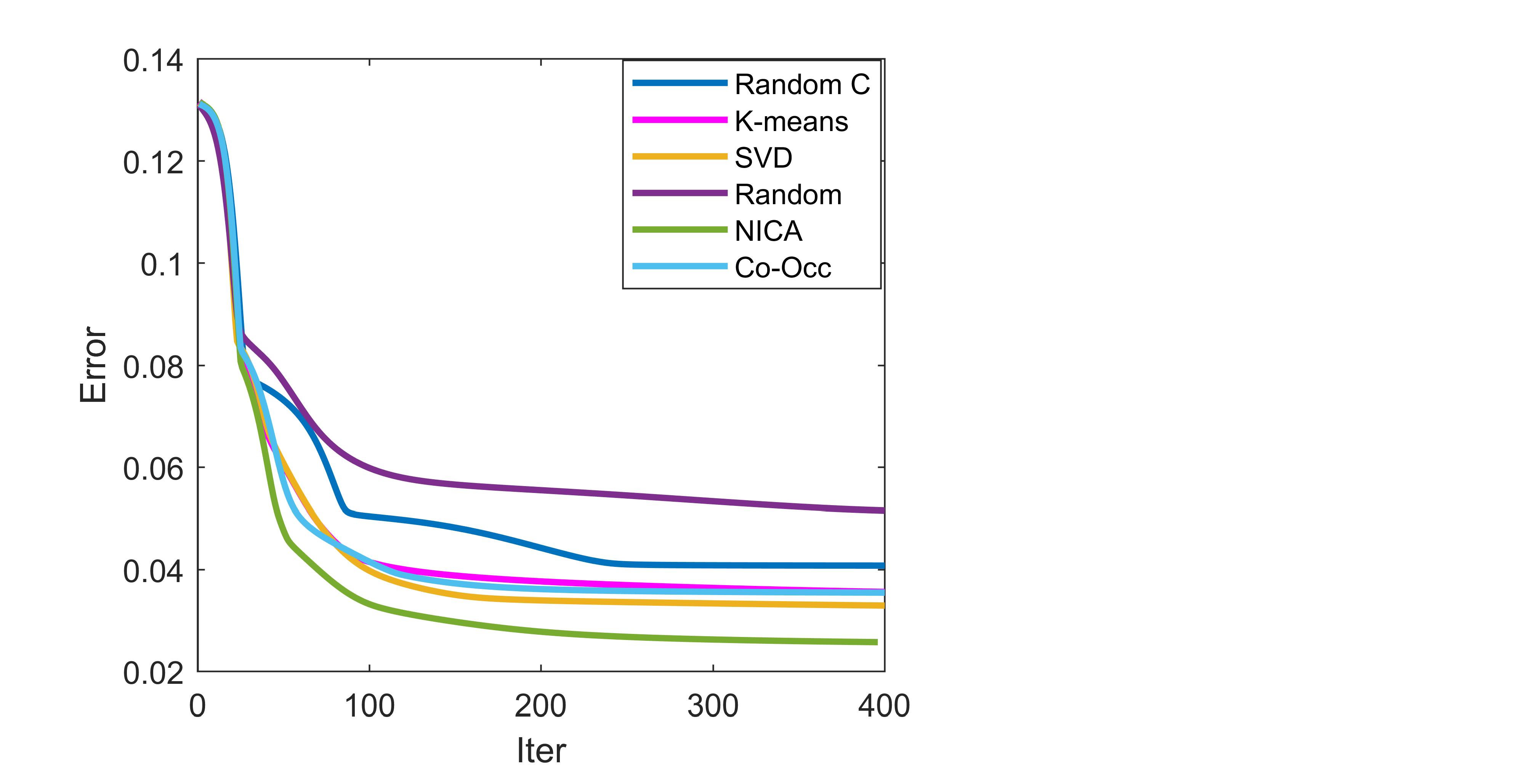
Figure 2: Number of training data is $320$.

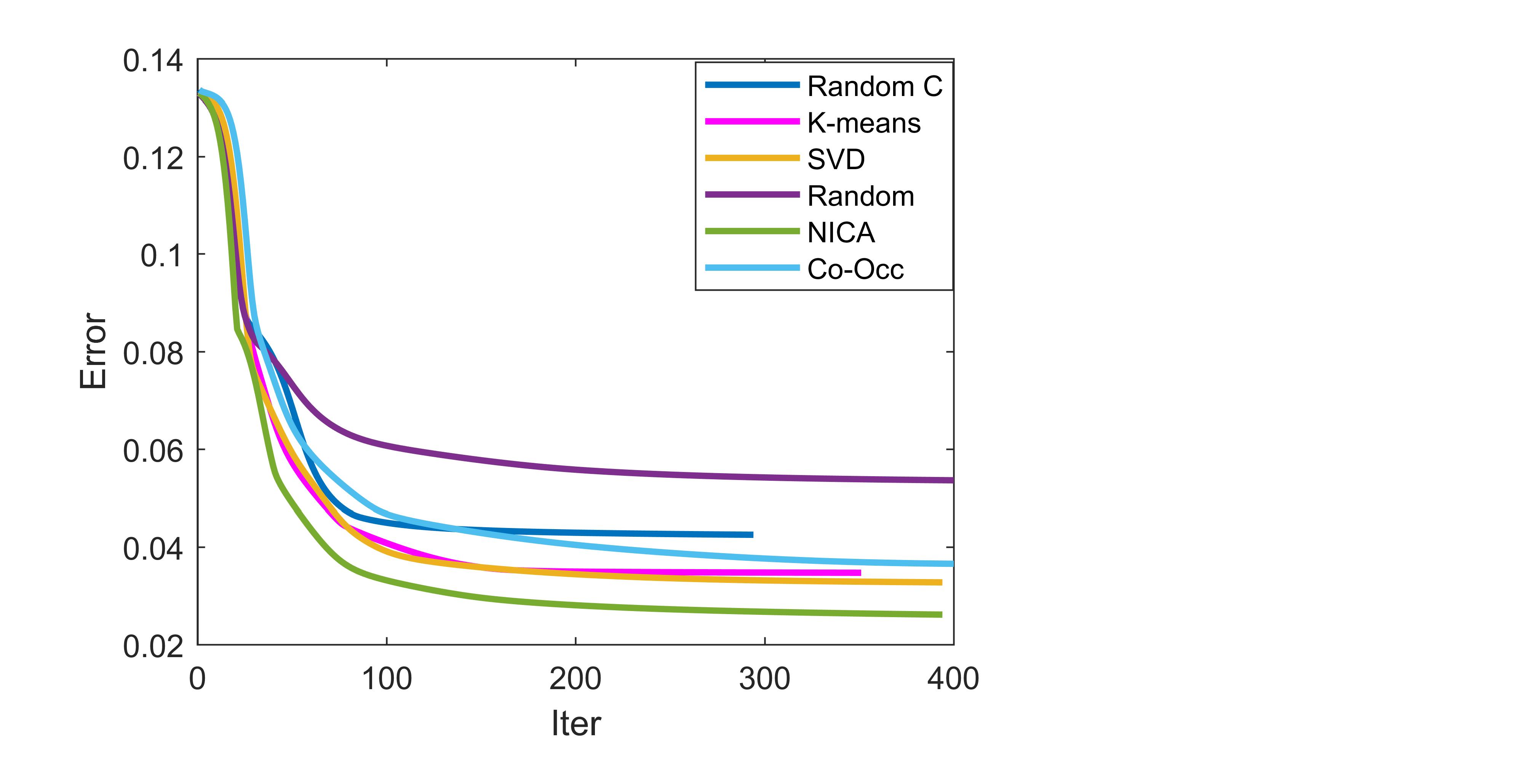
Figure 3: Number of training data is $200$.

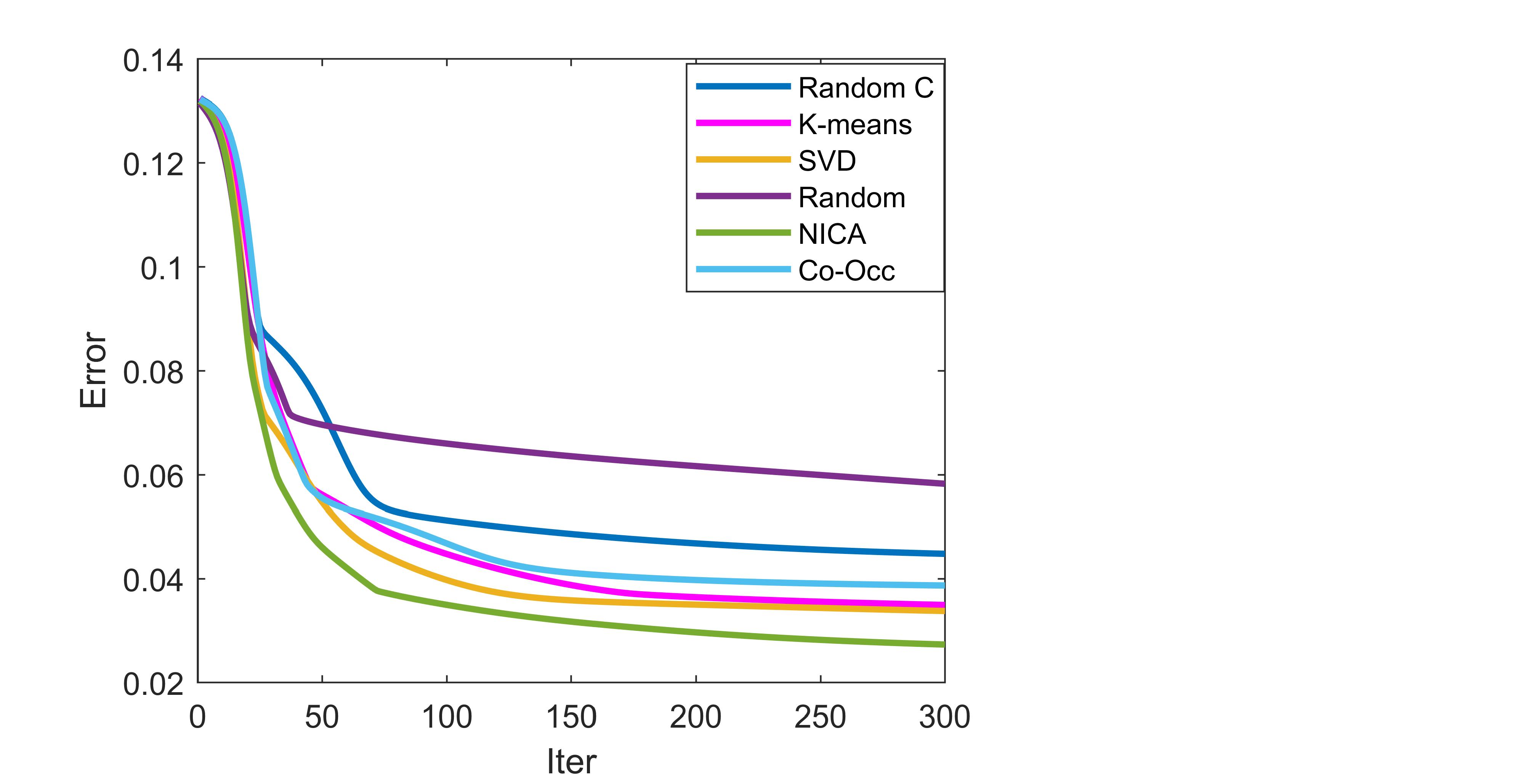
Figure 4: Number of training data is $120$.

As we see, the results of performing the algorithm with the NICA initialization approach are better than the other methods. In fact, this strategy improved the convergence results. This method has the best results for accuracy and the number of iterations. As shown in the figure, the NICA strategy has the best performance. In fact, the algorithm based on this method converges faster, and the value of error is the lowest. In fact, as mentioned before, the NICA method is not suitable for some datasets due to the production of orthogonal matrices. These results also show that although the random strategy is not expensive, its results are not as good as other methods.

8 Conclusion

In this paper, we studied various initialization strategies for NMF algorithms. In this direction, we first reviewed some common approaches for solving NMF. Then we calcified the initialization approaches for NMF. In fact, we divided these methods into four classes, that is, Random, Clastring, Heuristic, and Low-rank approximation methods. We summarize the advantages and disadvantages for some of them in Table 1. As we see that, the random strategies, that is, random, random Acol, and Random C are cheap are methods. On the other hand, NNDSVD, FC-Means, Co-occurrence, and k-means are expensive methods. The NNSVD-LRC is another method for initialization that is not expensive than SVD. NICA and NPCA are two other methods that have are not expensive as the K-means strategy but they have better results. Numerical results presented in this paper showed that NICA has better results than the other strategies in terms of error. In fact, we performed Lee’s Algorithm on ORL datasets with three different cases, that is, the number of training data is $\{120,200,320\}$. The NICA has the lowest error and this strategy leads the algorithm to converge faster than the other strategies.

Table 1: Advantages and disadvantages for initialization methods

$\begin{array}[]{ *{10}{c} }\hline\cr\hline\cr\text{name}&\text{Pros}&\text{Cons}\\ \hline\cr\pagecolor[gray]{0.8}\text{Random}&\text{easy}&\text{dense $(W^{0},H^{0})$}\\ \pagecolor[gray]{0.8}\hfil&\text{cheap to compute}&\text{with no intuitive meaning}&\\ \hline\cr\pagecolor[gray]{0.8}\text{Co-occurrence}&\text{uses term-term similarities}&\text{very expensive}\\ \hline\cr\hline\cr\pagecolor[gray]{0.8}\text{Random C }&\text{cheap }&\text{not very effective}\\ \hline\cr\hline\cr\pagecolor[gray]{0.8}\text{Random Aco}&\text{cheap }&\text{only slight decrease number of iterations}\\ \pagecolor[gray]{0.8}\hfil&\text{sparse matrices built from original data}&\\ \hline\cr\pagecolor[gray]{0.8}\text{k-means}&\text{reduces NMF iterations}&\text{dense}\\ \pagecolor[gray]{0.8}\hfil&\text{intuitive meaning of $W^{0}$}&\text{expensive}&\\ \hline\cr\pagecolor[gray]{0.8}\text{FC-means}&\text{intuitive meaning of $(W^{0},H^{0})$}&\text{dense $(W^{0},H^{0})$}&\\ \pagecolor[gray]{0.8}\hfil&&\text{expensive}\\ \hline\cr\pagecolor[gray]{0.8}\text{NNDSVD}&\text{no randomization;}&\text{expensive}\\ \hline\cr\hline\cr\pagecolor[gray]{0.8}\text{NNSVD-LRC}&\text{no randomization;}&\text{expensive}\\ \pagecolor[gray]{0.8}\hfil&\text{non-negative;}&\\ \hline\cr\hline\cr\hline\cr\hline\cr\end{array}$

Abbreviations

The following abbreviations are used in this paper:
NMF     Nonnegative matrix factorizations
LR        Low-rank
SVD     Singular Value Decomposition
PCA     Principal Component Analysis
KL        Kullback-Leiber
MU       Mutilplicative Update
NPCA     Non-negative PCA
ICA       Indipendent Component Analysis
NICA     non-negative ICA
NNDSVD     Non-negative Double SVD
NNSVD-LRC   Non-negative SVD LR Correction
FCM    Fuzzy C-means
DE       Differential Evolution
PSO     Particle Swarm Optimization

References

- Friedland et al. [2011] Shmuel Friedland, V Mehrmann, A Miedlar, and M Nkengla. Fast low rank approximations of matrices and tensors. The Electronic Journal of Linear Algebra, 22:1031–1048, 2011.
- Eldén [2003] Lars Eldén. Numerical linear algebra and applications in data mining and it. 2003.
- Skillicorn [2007] David Skillicorn. Understanding complex datasets: data mining with matrix decompositions. Chapman and Hall/CRC, 2007.
- Murphy [2012] Kevin P Murphy. Machine learning: a probabilistic perspective. MIT press, 2012.
- Lee et al. [2013] Joonseok Lee, Seungyeon Kim, Guy Lebanon, and Yoram Singer. Matrix approximation under local low-rank assumption. arXiv preprint arXiv:1301.3192, 2013.
- Golub and Van Loan [1996] Gene H Golub and Charles F Van Loan. Matrix computations 3rd edition. The John Hopkins University, Baltimore, 1996.
- Alter et al. [2000] Orly Alter, Patrick O Brown, and David Botstein. Singular value decomposition for genome-wide expression data processing and modeling. Proceedings of the National Academy of Sciences, 97(18):10101–10106, 2000.
- Wall et al. [2003] Michael E Wall, Andreas Rechtsteiner, and Luis M Rocha. Singular value decomposition and principal component analysis. In A practical approach to microarray data analysis, pages 91–109. Springer, 2003.
- Datta [2010] Biswa Nath Datta. Numerical linear algebra and applications, volume 116. Siam, 2010.
- Sundarapandian [2008] V Sundarapandian. Numerical linear algebra. PHI Learning Pvt. Ltd., 2008.
- Trefethen and Bau III [1997] Lloyd N Trefethen and David Bau III. Numerical linear algebra, volume 50. Siam, 1997.
- Recht et al. [2010] Benjamin Recht, Maryam Fazel, and Pablo A Parrilo. Guaranteed minimum-rank solutions of linear matrix equations via nuclear norm minimization. SIAM review, 52(3):471–501, 2010.
- Paruolo [2000] Paolo Paruolo. Multivariate reduced rank regression, theory and applications, 2000.
- Miller and de Callafon [2012] Daniel N Miller and Raymond A de Callafon. Identification of linear time-invariant systems via constrained step-based realization. IFAC Proceedings Volumes, 45(16):1155–1160, 2012.
- Chu et al. [2003] Moody T Chu, Robert E Funderlic, and Robert J Plemmons. Structured low rank approximation. Linear algebra and its applications, 366:157–172, 2003.
- Drineas et al. [2006] Petros Drineas, Ravi Kannan, and Michael W Mahoney. Fast monte carlo algorithms for matrices iii: Computing a compressed approximate matrix decomposition. SIAM Journal on Computing, 36(1):184–206, 2006.
- Smilde et al. [2005] Age Smilde, Rasmus Bro, and Paul Geladi. Multi-way analysis: applications in the chemical sciences. John Wiley & Sons, 2005.
- Meyer [2000] Carl D Meyer. Matrix analysis and applied linear algebra, volume 71. Siam, 2000.
- Kolda and O’leary [1998] Tamara G Kolda and Dianne P O’leary. A semidiscrete matrix decomposition for latent semantic indexing information retrieval. ACM Transactions on Information Systems (TOIS), 16(4):322–346, 1998.
- Esposito et al. [2021] Flavia Esposito, Nicoletta Del Buono, and Laura Selicato. Nonnegative matrix factorization models for knowledge extraction from biomedical and other real world data. PAMM, 20(1):e202000032, 2021.
- Meng et al. [2016] Chen Meng, Oana A Zeleznik, Gerhard G Thallinger, Bernhard Kuster, Amin M Gholami, and Aedín C Culhane. Dimension reduction techniques for the integrative analysis of multi-omics data. Briefings in bioinformatics, 17(4):628–641, 2016.
- Sompairac et al. [2019] Nicolas Sompairac, Petr V Nazarov, Urszula Czerwinska, Laura Cantini, Anne Biton, Askhat Molkenov, Zhaxybay Zhumadilov, Emmanuel Barillot, Francois Radvanyi, Alexander Gorban, et al. Independent component analysis for unraveling the complexity of cancer omics datasets. International Journal of molecular sciences, 20(18):4414, 2019.
- Lee and Seung [1999] Daniel D Lee and H Sebastian Seung. Learning the parts of objects by non-negative matrix factorization. Nature, 401(6755):788–791, 1999.
- Aggarwal and Reddy [2014] Charu C Aggarwal and Chandan K Reddy. Data clustering. Algorithms and applications. Chapman&Hall/CRC Data mining and Knowledge Discovery series, Londra, 2014.
- [25] DD Lee and HS Seung. Algorithms for non-negative matrix factorization. nips (2000). Google Scholar, pages 556–562.
- Boutsidis and Gallopoulos [2008] Christos Boutsidis and Efstratios Gallopoulos. Svd based initialization: A head start for nonnegative matrix factorization. Pattern recognition, 41(4):1350–1362, 2008.
- Casalino et al. [2014] Gabriella Casalino, Nicoletta Del Buono, and Corrado Mencar. Subtractive clustering for seeding non-negative matrix factorizations. Information Sciences, 257:369–387, 2014.
- Esposito [2021] Flavia Esposito. A review on initialization methods for nonnegative matrix factorization: Towards omics data experiments. Mathematics, 9(9):1006, 2021.
- Gong and Zhang [2012] Pinghua Gong and Changshui Zhang. Efficient nonnegative matrix factorization via projected newton method. Pattern Recognition, 45(9):3557–3565, 2012.
- Bonettini et al. [2008] Silvia Bonettini, Riccardo Zanella, and Luca Zanni. A scaled gradient projection method for constrained image deblurring. Inverse problems, 25(1):015002, 2008.
- Guan et al. [2012] Naiyang Guan, Dacheng Tao, Zhigang Luo, and Bo Yuan. Nenmf: An optimal gradient method for nonnegative matrix factorization. IEEE Transactions on Signal Processing, 60(6):2882–2898, 2012.
- Huang et al. [2015] Yakui Huang, Hongwei Liu, and Shuisheng Zhou. Quadratic regularization projected barzilai–borwein method for nonnegative matrix factorization. Data mining and knowledge discovery, 29(6):1665–1684, 2015.
- Fathi-Hafshejani and Moaberfard [2020] S Fathi-Hafshejani and Z Moaberfard. An interior-point algorithm for linearly constrained convex optimization based on kernel function and application in non-negative matrix factorization. Optimization and Engineering, 21(3):1019–1051, 2020.
- Albright et al. [2006] Russell Albright, James Cox, David Duling, Amy N Langville, and C Meyer. Algorithms, initializations, and convergence for the nonnegative matrix factorization. Technical report, Tech. rep. 919. NCSU Technical Report Math 81706. http://meyer. math. ncsu …, 2006.
- Zheng et al. [2007] Zhonglong Zheng, Jie Yang, and Yitan Zhu. Initialization enhancer for non-negative matrix factorization. Engineering Applications of Artificial Intelligence, 20(1):101–110, 2007.
- Xue et al. [2008] Yun Xue, Chong Sze Tong, Ying Chen, and Wen-Sheng Chen. Clustering-based initialization for non-negative matrix factorization. Applied Mathematics and Computation, 205(2):525–536, 2008.
- Alshabrawy et al. [2012] Ossama S Alshabrawy, ME Ghoneim, WA Awad, and Aboul Ella Hassanien. Underdetermined blind source separation based on fuzzy c-means and semi-nonnegative matrix factorization. In 2012 Federated Conference on Computer Science and Information Systems (FedCSIS), pages 695–700. IEEE, 2012.
- Rezaei et al. [2011] M Rezaei, R Boostani, and M Rezaei. An efficient initialization method for nonnegative matrix factorization. Journal of Applied Sciences, 11(2):354–359, 2011.
- Kim and Choi [2007] Yong-Deok Kim and Seungjin Choi. A method of initialization for nonnegative matrix factorization. In 2007 IEEE International Conference on Acoustics, Speech and Signal Processing-ICASSP’07, volume 2, pages II–537. IEEE, 2007.
- Stadlthanner et al. [2007] Kurt Stadlthanner, Dominik Lutter, Fabian J Theis, Elmar Wolfgang Lang, Ana Maria Tomé, Petia Georgieva, and Carlos García Puntonet. Sparse nonnegative matrix factorization with genetic algorithms for microarray analysis. In 2007 International Joint Conference on Neural Networks, pages 294–299. IEEE, 2007.
- Snášel et al. [2008a] Václav Snášel, Jan Platoš, and Pavel Krömer. Developing genetic algorithms for boolean matrix factorization. Databases, Texts, 61, 2008a.
- Price et al. [2006] Kenneth Price, Rainer M Storn, and Jouni A Lampinen. Differential evolution: a practical approach to global optimization. Springer Science & Business Media, 2006.
- Atif et al. [2019] Syed Muhammad Atif, Sameer Qazi, and Nicolas Gillis. Improved svd-based initialization for nonnegative matrix factorization using low-rank correction. Pattern Recognition Letters, 122:53–59, 2019.
- Zhao et al. [2008] Lihong Zhao, Guibin Zhuang, and Xinhe Xu. Facial expression recognition based on pca and nmf. In 2008 7th World Congress on Intelligent Control and Automation, pages 6826–6829. IEEE, 2008.
- Kitamura and Ono [2016] Daichi Kitamura and Nobutaka Ono. Efficient initialization for nonnegative matrix factorization based on nonnegative independent component analysis. In 2016 IEEE International Workshop on Acoustic Signal Enhancement (IWAENC), pages 1–5. IEEE, 2016.
- Oja and Plumbley [2004] Erkki Oja and Mark Plumbley. Blind separation of positive sources by globally convergent gradient search. Neural Computation, 16(9):1811–1825, 2004.
- Benachir et al. [2013] Djaouad Benachir, Shahram Hosseini, Yannick Deville, Moussa Sofiane Karoui, and Abdelkader Hameurlain. Modified independent component analysis for initializing non-negative matrix factorization: An approach to hyperspectral image unmixing. In 2013 IEEE 11th International Workshop of Electronics, Control, Measurement, Signals and their application to Mechatronics, pages 1–6. IEEE, 2013.
- Sandler [2005] Mark Sandler. On the use of linear programming for unsupervised text classification. In Proceedings of the eleventh ACM SIGKDD international conference on Knowledge discovery in data mining, pages 256–264, 2005.
- Liu and Tan [2018] Zhaoqiang Liu and Vincent YF Tan. Rank-one nmf-based initialization for nmf and relative error bounds under a geometric assumption. In 2018 Information Theory and Applications Workshop (ITA), pages 1–15. IEEE, 2018.
- Zdunek [2012] Rafal Zdunek. Initialization of nonnegative matrix factorization with vertices of convex polytope. In International Conference on Artificial Intelligence and Soft Computing, pages 448–455. Springer, 2012.
- Sauwen et al. [2017] Nicolas Sauwen, Marjan Acou, Halandur N Bharath, Diana M Sima, Jelle Veraart, Frederik Maes, Uwe Himmelreich, Eric Achten, and Sabine Van Huffel. The successive projection algorithm as an initialization method for brain tumor segmentation using non-negative matrix factorization. Plos one, 12(8):e0180268, 2017.
- Mahoney [2011] Michael W Mahoney. Randomized algorithms for matrices and data. arXiv preprint arXiv:1104.5557, 2011.
- Drineas and Mahoney [2016] Petros Drineas and Michael W Mahoney. Randnla: randomized numerical linear algebra. Communications of the ACM, 59(6):80–90, 2016.
- Wang and Li [2010] Fei Wang and Ping Li. Efficient nonnegative matrix factorization with random projections. In Proceedings of the 2010 SIAM International Conference on Data Mining, pages 281–292. SIAM, 2010.
- Tepper and Sapiro [2016] Mariano Tepper and Guillermo Sapiro. Compressed nonnegative matrix factorization is fast and accurate. IEEE Transactions on Signal Processing, 64(9):2269–2283, 2016.
- Langville et al. [2006] Amy N Langville, Carl D Meyer, Russell Albright, James Cox, and David Duling. Alternating least squares algorithms for the nonnegative matrix factorization, 2006.
- Berthold et al. [2010] Michael R Berthold, Christian Borgelt, Frank Höppner, and Frank Klawonn. Guide to intelligent data analysis: how to intelligently make sense of real data. Springer Science & Business Media, 2010.
- Xu et al. [2003] Wei Xu, Xin Liu, and Yihong Gong. Document clustering based on non-negative matrix factorization. In Proceedings of the 26th annual international ACM SIGIR conference on Research and development in informaion retrieval, pages 267–273, 2003.
- Chrétien et al. [2016] Stéphane Chrétien, Christophe Guyeux, Bastien Conesa, Régis Delage-Mouroux, Michèle Jouvenot, Philippe Huetz, and Françoise Descôtes. A bregman-proximal point algorithm for robust non-negative matrix factorization with possible missing values and outliers-application to gene expression analysis. BMC bioinformatics, 17(8):623–631, 2016.
- Cichocki and Amari [2002] Andrzej Cichocki and Shun-ichi Amari. Adaptive blind signal and image processing: learning algorithms and applications. John Wiley & Sons, 2002.
- Perronnin and Bouchard [2017] Florent Perronnin and Guillaume Bouchard. Clustering using non-negative matrix factorization on sparse graphs, August 8 2017. US Patent 9,727,532.
- Wild et al. [2004] Stefan Wild, James Curry, and Anne Dougherty. Improving non-negative matrix factorizations through structured initialization. Pattern recognition, 37(11):2217–2232, 2004.
- Wild et al. [2003] Stefan Wild, Written Stefan Wild, James Curry, Anne Dougherty, and Meredith Betterton. Seeding non-negative matrix factorizations with the spherical k-means clustering. PhD thesis, Citeseer, 2003.
- Forgey [1965] Edward Forgey. Cluster analysis of multivariate data: Efficiency vs. interpretability of classification. Biometrics, 21(3):768–769, 1965.
- Hartigan [1975] John A Hartigan. Clustering algorithms. John Wiley & Sons, Inc., 1975.
- [66]
- Anderberg [2014] Michael R Anderberg. Cluster analysis for applications: probability and mathematical statistics: a series of monographs and textbooks, volume 19. Academic press, 2014.
- Dong et al. [2014] Bo Dong, Matthew M Lin, and Moody T Chu. Nonnegative rank factorization—a heuristic approach via rank reduction. Numerical Algorithms, 65(2):251–274, 2014.
- Goldberg and Holland [1988] David E Goldberg and John Henry Holland. Genetic algorithms and machine learning. 1988.
- Snášel et al. [2008b] Václav Snášel, Jan Platoš, and Pavel Krömer. Developing genetic algorithms for boolean matrix factorization. Databases, Texts, 61, 2008b.
- Eberhart and Kennedy [1995] Russell Eberhart and James Kennedy. Particle swarm optimization. In Proceedings of the IEEE international conference on neural networks, volume 4, pages 1942–1948. Citeseer, 1995.
- Janecek and Tan [2011] Andreas Janecek and Ying Tan. Using population based algorithms for initializing nonnegative matrix factorization. In International Conference in Swarm Intelligence, pages 307–316. Springer, 2011.
- Deerwester et al. [1990] Scott Deerwester, Susan T Dumais, George W Furnas, Thomas K Landauer, and Richard Harshman. Indexing by latent semantic analysis. Journal of the American society for information science, 41(6):391–407, 1990.
- Eckart and Young [1936] Carl Eckart and Gale Young. The approximation of one matrix by another of lower rank. Psychometrika, 1(3):211–218, 1936.
- Cao [2006] Lijie Cao. Singular value decomposition applied to digital image processing. Division of Computing Studies, Arizona State University Polytechnic Campus, Mesa, Arizona State University polytechnic Campus, pages 1–15, 2006.
- Cichocki et al. [2009] Andrzej Cichocki, Rafal Zdunek, Anh Huy Phan, and Shun-ichi Amari. Nonnegative matrix and tensor factorizations: applications to exploratory multi-way data analysis and blind source separation. John Wiley & Sons, 2009.
- Guillamet and Vitria [2003] David Guillamet and Jordi Vitria. Evaluation of distance metrics for recognition based on non-negative matrix factorization. Pattern Recognition Letters, 24(9-10):1599–1605, 2003.
- Turk and Pentland [1991] Matthew Turk and Alex Pentland. Eigenfaces for recognition. Journal of cognitive neuroscience, 3(1):71–86, 1991.
- Geng et al. [2016] Xiu-rui Geng, Lu-yan Ji, and Kang Sun. Non-negative matrix factorization based unmixing for principal component transformed hyperspectral data. Frontiers of Information Technology & Electronic Engineering, 17(5):403–412, 2016.
- Shen and Huang [2008] Haipeng Shen and Jianhua Z Huang. Sparse principal component analysis via regularized low rank matrix approximation. Journal of multivariate analysis, 99(6):1015–1034, 2008.
- Zass and Shashua [2007] Ron Zass and Amnon Shashua. Nonnegative sparse pca. In Advances in neural information processing systems, pages 1561–1568. Citeseer, 2007.
- Bauckhage [2014] Christian Bauckhage. A purely geometric approach to non-negative matrix factorization. In LWA, pages 125–136. Citeseer, 2014.
- Smaragdis et al. [2006] Paris Smaragdis, Bhiksha Raj, and Madhusudana Shashanka. A probabilistic latent variable model for acoustic modeling. Advances in models for acoustic processing, NIPS, 148:8–1, 2006.