Recurrent Neural Network Controllers Synthesis with Stability Guarantees for Partially Observed Systems

Abstract

Neural network controllers have become popular in control tasks thanks to their flexibility and expressivity. Stability is a crucial property for safety-critical dynamical systems, while stabilization of partially observed systems, in many cases, requires controllers to retain and process long-term memories of the past. We consider the important class of recurrent neural networks (RNN) as dynamic controllers for nonlinear uncertain partially-observed systems, and derive convex stability conditions based on integral quadratic constraints, S-lemma and sequential convexification. To ensure stability during the learning and control process, we propose a projected policy gradient method that iteratively enforces the stability conditions in the reparametrized space taking advantage of mild additional information on system dynamics. Numerical experiments show that our method learns stabilizing controllers while using fewer samples and achieving higher final performance compared with policy gradient.

1 Introduction

Neural network decision making and control has seen a huge advancement recently accompanied by the success of reinforcement learning (RL) (Sutton and Barto 2018). In particular, deep reinforcement learning (DRL) has achieved super-human performance with neural network policies (also referred to as controllers in control tasks) in various domains (Mnih et al. 2015; Lillicrap et al. 2016; Silver et al. 2016).

Policy gradient (Sutton et al. 1999) is one of the most important approaches to DRL that synthesizes policies for continuous decision making problems. For control tasks, policy gradient method and its variants have successfully synthesized neural network controllers to accomplish complex control goals (Levine et al. 2018) without solving potentially non-linear planing problems at test time (Levine et al. 2016). However, most of these methods focus on maximizing the reward function which only indirectly enforce desirable properties. Specifically, global stability of the closed-loop system (Sastry 2013) guarantees convergence to the desired state of origin from any initial state and therefore is a very important property for safety critical systems (e.g.  aircraft control (Chakraborty, Seiler, and Balas 2011)) where not a single diverging trajectory is acceptable. However, the set of parameters corresponding to stabilizing controllers is in general nonconvex even in the simple setting of linear systems with linear controllers (Fazel et al. 2018), which poses significant computational challenges for neural network controllers under the general setting of nonlinear systems.

Thanks to recent robustness studies of deep learning, we have seen attempts on giving stability certificates and/or ensuring stability at test time for fully-observed systems controlled by neural networks. Yet stability problems for neural network controlled partially observed systems remain open. Unlike fully-observed control systems where the plant states are fully revealed to the controller, most real-world control systems are only partially observed due to modeling inaccuracy, sensing limitations, and physical constraints (Braziunas 2003). Here, sensible estimates of the full system state usually depend on historical observations (Callier and Desoer 2012). Some partially observed systems are modeled using partially observed Markov decision process (POMDP) (Monahan 1982) where an optimal solution is NP hard in general (Mundhenk et al. 2000).

Paper contributions. In the paper, we propose a method to synthesize recurrent neural network (RNN) controllers with exponential stability guarantees for partially observed systems. We derive a convex inner approximation to the non-convex set of stable RNN parameters based on integral quadratic constraints (Megretski and Rantzer 1997), loop transformation (Sastry 2013, Chap. 4) and a sequential semidefinite convexification technique, which guarantees exponential stability for both linear time invariant (LTI) systems and general nonlinear uncertain systems. A novel framework of projected policy gradient is proposed to maximize some unknown/complex reward function and ensure stability in the online setting where a guaranteed-stable RNN controller is synthesized and iteratively updated while interacting with and controlling the underlying system, which differentiates our works from most post-hoc validation methods. Finally, we carry out comprehensive comparisons with policy gradient, and demonstrate that our method effectively ensures the closed-loop stability and achieves higher reward on a variety of control tasks, including vehicle lateral control and power system frequency regulation.

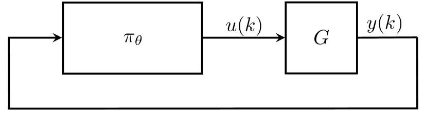
Figure 1: Feedback system of plant $G$ and RNN controller $\pi_{\theta}$

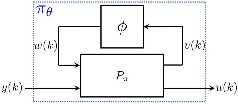
Figure 2: RNN as an interconnection of $P_{\pi}$ and $\phi$

Paper outline. In Section 2, we outline related works on addressing partial observability, and enforcing stability in reinforcement learning. Section 3 discusses our proposed method for synthesizing RNN controllers for LTI plants with stability guarantees, and Section 4 extends it to systems with uncertainties and nonlinearities. Section 5 compares the proposed projected policy gradient method with policy gradient through numerical experiments.

Notation. $\mathbb{S}^{n},\mathbb{S}^{n}_{+},\mathbb{S}^{n}_{++}$ denote the sets of $n$-by-$n$ symmetric, positive semidefinite and positive definite matrices, respectively. $\mathbb{D}^{n}_{+}$, $\mathbb{D}^{n}_{++}$ denote the set of $n$-by-$n$ diagonal positive semidefinite, and diagonal positive definite matrices. The notation $\|\cdot\|:\mathbb{R}^{n}\rightarrow\mathbb{R}$ denotes the standard 2-norm. We define $\ell_{2e}^{n}$ to be the set of all one-sided sequences $x:\mathbb{N}\rightarrow\mathbb{R}^{n}$. The subset $\ell_{2}^{n}\subset\ell_{2e}^{n}$ consists of all square-summable sequences. When applied to vectors, the orders $>,\leq$ are applied elementwise.

2 Related Work

Partially Observed Decision Making and Output Feedback Control. In many problems (Talpaert et al. 2019; Barto, Bradtke, and Singh 1995), only specific outputs but not the full system states are available for the decision maker. Therefore, memory in the controller is required to recover the full system states (Scherer, Gahinet, and Chilali 1997). Control of these partially observed systems is often referred to as output feedback control (Callier and Desoer 2012), and has been studied extensively from both control and optimization perspectives (Doyle 1978; Zheng, Tang, and Li 2021). Under the setting with convexifiable objectives (e.g., $H_{\infty}$ or $H_{2}$ performances), the optimal linear dynamic (i.e.  with memory) controller can be obtained by using a change of variables or solving algebraic Riccati equations (Gahinet and Apkarian 1994; Zhou et al. 1996). However, for more sophisticated settings with unknown and/or flexibly defined cost functions, the problems become intractable for the aforementioned traditional methods, and RL techniques are proposed to reduced the computation cost and improve overall performance at test time, including the ones (Levine and Koltun 2013; Levine et al. 2016) with static neural network controllers, and the ones (Zhang et al. 2016; Heess et al. 2015; Wierstra et al. 2007) with dynamic controllers, represented by RNNs/long short-term memory neural networks.

Stability Guarantees For Neural Network Controlled Systems. As neural networks become popular in control tasks, safety and robustness of neural networks and neural network controlled systems has been actively discussed (Morimoto and Doya 2005; Luo, Wu, and Huang 2014; Friedrich and Buss 2017; Berkenkamp et al. 2017; Chow et al. 2018; Matni et al. 2019; Han et al. 2019; Recht 2019; Choi et al. 2020; Zhang, Hu, and Basar 2020; Fazlyab, Morari, and Pappas 2020). Closely related to this work are recent papers on robustness analysis of memory-less neural networks controlled systems based on robust control ideas. Yin, Seiler, and Arcak (2021); Yin et al. (2021); Pauli et al. (2021); Jin and Lavaei (2020) conduct stability analysis of neural network controlled linear and nonlinear systems and propose verification methods by characterizing activation functions using quadratic constraints. Donti et al. (2020) adds additional projection layer on the controller to ensure stability for fully observed systems. (Revay, Wang, and Manchester 2020) studies the stability of RNN itself when fitted to data but does not consider any plant to control by such RNN. The most related works are those that study dynamic neural network controllers. Anderson et al. (2007); Knight and Anderson (2011) adapt RNN controllers through RL techniques to obtain stability guarantees. However, in these works, the reward function is assumed to be known, and conservative updates of controller parameters projected to a box neighborhood of the previous iterate are applied due to the non-convexity in their conditions. In contrast, our work enables much larger and more efficient updates thanks to jointly convex conditions derived through a novel sequential convexification and loop transformation approach unseen in these works.

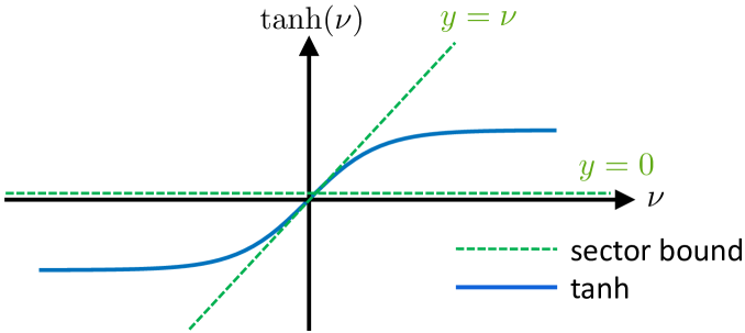
Figure 3: $\tanh\in$ sector $[0,1]$,
Leaky ReLU $\in$ sector $[a,1]$

Figure 4: Loop transformation. If $\phi\in$ sector $[\alpha_{\phi},\beta_{\phi}]$, then $\tilde{\phi}\in$ sector $[-1_{n_{\phi}\times 1},1_{n_{\phi}\times 1}]$.

3 Partially Observed Linear Systems

Problem Formulation

Consider the feedback system (shown in Fig. 2) consisting of a plant $G$ and an RNN controller $\pi_{\theta}$ which is expected to stabilize the system (i.e. steer the states of $G$ to the origin). To streamline the presentation, we consider a partially observed, linear, time-invariant (LTI) system $G$ defined by the following discrete-time model:

$$x(k+1) =A_{G}\ x(k)+B_{G}\ u(k)$$ (1a)

$$y(k) =C_{G}\ x(k)$$ (1b)

where $x(k)\in\mathbb{R}^{n_{G}}$ is the state, $u(k)\in\mathbb{R}^{n_{u}}$ is the control input, and $y(k)\in\mathbb{R}^{n_{y}}$ is the output. $A_{G}\in\mathbb{R}^{n_{G}\times n_{G}}$, $B_{G}\in\mathbb{R}^{n_{G}\times n_{u}}$, and $C_{G}\in\mathbb{R}^{n_{y}\times n_{G}}$. Since the plant $G$ is partially observed, the observation matrix $C_{G}$ may have a sparsity pattern or be column-rank deficient.

Assumption 1.

We assume that $(A_{G},B_{G})$ is stabilizable, and $(A_{G},C_{G})$ is detectable.

Assumption 2.

We assume $A_{G},B_{G},$ and $C_{G}$ are known.

Assumption 2 is partially lifted in Section 4 where we only assume partial information on the system dynamics.

Problem 1.

Our goal is to find a controller $\pi$ that maps the observation $y$ to an action $u$ to both maximize some unknown reward $R=\sum_{k=0}^{T}r_{k}(x(k),u(k))$ over finite horizon $T$ and stabilize the plant $G$.

The single step reward $r_{k}(x(k),u(k))$ is assumed to be unknown and potentially highly complex to capture the vast possibility of desired controller. e.g. In many cases, to ensure extra safety, the reward is set to $r_{k}(x(k),u(k))=0,\forall k\geq l$ if there is a state violation at step $l$. This cannot be captured by any simple negative quadratic functions.

Controllers Parameterization

Output feedback control with known and convexifiable reward has been studied extensively (Scherer, Gahinet, and Chilali 1997), and linear dynamic controllers suffice for this case. However, in our problem setting, since the reward is unknown and nonconvex, and systems dynamics will become uncertain and nonlinear in Section 4, we consider a dynamic controller in the form of an RNN, which makes a class of high-capacity flexible controllers.

We model the RNN controller $\pi_{\theta}$ as an interconnection of an LTI system $P_{\pi}$, and combined activation functions $\phi:\mathbb{R}^{n_{\phi}}\rightarrow\mathbb{R}^{n_{\phi}}$ as shown in Fig. 2. This parameterization is expressive, and contains many widely used model structures (Revay, Wang, and Manchester 2020). The RNN $\pi_{\theta}$ is defined as follows

$$P_{\pi}\left\{\begin{array}[]{ll}\xi(k+1)&=A_{K}\ \xi(k)\ +B_{K1}\ w(k)+B_{K2}\ y(k)\\ u(k)&=C_{K1}\ \xi(k)+D_{K1}\ w(k)+D_{K2}\ y(k)\\ v(k)&=C_{K2}\ \xi(k)+D_{K3}\ y(k)\end{array}\right.$$ (5)

$$\hskip 24.75375ptw(k)\hskip 24.18501pt=\phi(v(k))$$ (6)

where $\xi\in\mathbb{R}^{n_{\xi}}$ is the hidden state, $v,w\in\mathbb{R}^{n_{\phi}}$ are the input and output of $\phi$, and matrices $A_{K},\dots,D_{K3}$ are parameters to be learned. Define $\theta=\left[\begin{smallmatrix}A_{K}&B_{K1}&B_{K2}\\ C_{K1}&D_{K1}&D_{K2}\\ C_{K2}&0&D_{K3}\end{smallmatrix}\right]$ as the collection of the learnable parameters of $\pi_{\theta}$. We assume the initial condition of $\xi$ to be zero $\xi(0)=0_{n_{\xi}\times 1}$. The combined nonlinearity $\phi$ is applied element-wise, i.e., $\phi:=[\varphi_{1}(v_{1}),...,\varphi_{n_{\phi}}(v_{n_{\phi}})]^{\top}$, where $\varphi_{i}$ is the $i$-th scalar activation function. We assume that the activation has a fixed point at origin, i.e. $\phi(0)=0$.

Quadratic Constraints for Activation Functions

The stability condition relies on quadratic constraints (QCs) to bound the activation function. A typical QC is the sector bound as defined next.

Definition 3.1.

Let $\alpha\leq\beta$ be given. The function $\varphi:\mathbb{R}\rightarrow\mathbb{R}$ lies in the sector $[\alpha,\beta]$ if:

$$(\varphi(\nu)-\alpha\nu)\cdot(\beta\nu-\varphi(\nu))\geq 0\,\,\,\forall\nu\in\mathbb{R}.$$ (7)

The interpretation of the sector $[\alpha,\beta]$ is that $\varphi$ lies between lines passing through the origin with slope $\alpha$ and $\beta$. Many activations are sector bounded, e.g., leaky ReLU is sector bounded in $[a,1]$ with its parameter $a\in(0,1)$; ReLU and $\tanh$ are sector bounded in $[0,1]$ (denoted as $\tanh\in$ sector $[0,1]$). Fig. 4 illustrates different activations (blue solid) and their sector bounds (green dashed).

Sector constraints can also be defined for combined activations $\phi$. Assume the $i$-th scalar activation $\varphi_{i}$ in $\phi$ is sector bounded by $[\alpha_{i},\beta_{i}]$, $i=1,...,n_{\phi}$, then these sectors can be stacked into vectors $\alpha_{\phi},\beta_{\phi}\in\mathbb{R}^{n_{\phi}}$, where $\alpha_{\phi}=[\alpha_{1},...,\alpha_{n_{\phi}}]$ and $\beta_{\phi}=[\beta_{1},...,\beta_{n_{\phi}}]$, to provide QCs satisfied by $\phi$.

Lemma 3.1.

Let $\alpha_{\phi},\beta_{\phi}\in\mathbb{R}^{n_{\phi}}$ be given with $\alpha_{\phi}\leq\beta_{\phi}$. Suppose that $\phi$ satisfies the sector bound $[\alpha_{\phi},\beta_{\phi}]$ element-wise. For any $\Lambda\in\mathbb{D}_{+}^{n_{\phi}}$, and for all $v\in\mathbb{R}^{n_{\phi}}$ and $w=\phi(v)$, it holds that

$$\begin{bmatrix}v\\ w\end{bmatrix}^{\top}\begin{bmatrix}-2A_{\phi}B_{\phi}\Lambda&(A_{\phi}+B_{\phi})\Lambda\\ (A_{\phi}+B_{\phi})\Lambda&-2\Lambda\end{bmatrix}\begin{bmatrix}v\\ w\end{bmatrix}\geq 0,$$ (8)

where $A_{\phi}=diag(\alpha_{\phi})$, and $B_{\phi}=diag(\beta_{\phi})$.

A proof is available in (Fazlyab, Morari, and Pappas 2020).

Loop Transformation

To derive convex stability conditions for their efficient enforcement in the learning process, we first perform a loop transformation on the RNN as shown in Fig. 4. Through loop transformation, we obtain a new representation of the controller $\pi_{\tilde{\theta}}$, which is equivalent to the one shown in Fig. 2:

$$\begin{bmatrix}v\\ u\end{bmatrix} =\tilde{P}_{\pi}\begin{bmatrix}z\\ y\end{bmatrix}$$ (9a)

$$z(k) =\tilde{\phi}(v(k)).$$ (9b)

The newly obtained nonlinearity $\tilde{\phi}$, defined in Fig. 4, is sector bounded by $[-1_{n_{\phi}\times 1},1_{n_{\phi}\times 1}]$, and thus it satisfies a simplified QC: for any $\Lambda\in\mathbb{D}_{+}^{n_{\phi}}$, it holds that

$$\begin{bmatrix}v\\ z\end{bmatrix}^{\top}\begin{bmatrix}\Lambda&0\\ 0&-\Lambda\end{bmatrix}\begin{bmatrix}v\\ z\end{bmatrix}\geq 0,\ \forall v\in\mathbb{R}^{n_{\phi}}\ \text{and}\ z=\tilde{\phi}(v).$$ (10)

The transformed system $\tilde{P}_{\pi}$, defined in Fig. 4, is of the form:

$$\begin{array}[]{ll}\xi(k+1)&=\tilde{A}_{K}~{}~{}\xi(k)+B_{K1}\frac{B_{\phi}-A_{\phi}}{2}\ z(k)+\tilde{B}_{K2}\ y(k)\\ u(k)&=\tilde{C}_{K1}\ \xi(k)+D_{K1}\frac{B_{\phi}-A_{\phi}}{2}\ z(k)+\tilde{D}_{K2}\ y(k)\\ v(k)&=C_{K2}\ \xi(k)+D_{K3}\ y(k)\end{array}$$

where

$$\begin{array}[]{l}\hskip 3.41418pt\tilde{A}_{K}=A_{K}+B_{K1}S_{\phi}C_{K2},\hskip 8.5359pt\tilde{B}_{K2}=B_{K2}+B_{K1}S_{\phi}D_{K3},\\ \tilde{C}_{K1}=C_{K1}+D_{K1}S_{\phi}C_{K2},\hskip 4.26773pt\tilde{D}_{K2}=D_{K2}+D_{K1}S_{\phi}D_{K3},\end{array}$$ (13)

$$\hskip 85.35826ptS_{\phi}:=\textstyle\frac{A_{\phi}+B_{\phi}}{2}.$$ (14)

The derivation of $\tilde{P}_{\pi}$ can be found in Appendix A. We define the learnable parameters of $\pi_{\tilde{\theta}}$ as $\tilde{\theta}=\left[\begin{smallmatrix}\tilde{A}_{K}&B_{K1}&\tilde{B}_{K2}\\ \tilde{C}_{K1}&D_{K1}&\tilde{D}_{K2}\\ C_{K2}&0&D_{K3}\end{smallmatrix}\right]$. Since there is an one-to-one correspondence (14) between the transformed parameters $\tilde{\theta}$ and the original parameters $\theta$, we will learn in the reparameterized space and uniquely recover the original parameters accordingly.

Convex Lyapunov Condition

The feedback system of plant $G$ and RNN controller in $\pi_{\tilde{\theta}}$ (9) is defined by the following equations

$$\zeta(k+1) =\mathcal{A}\ \zeta(k)+\mathcal{B}\ z(k)$$ (15a)

$$v(k) =\ \mathcal{C}\ \zeta(k)+\mathcal{D}\ z(k)$$ (15b)

$$z(k) =\tilde{\phi}(v(k))$$ (15c)

where $\zeta=[x^{\top},\ \xi^{\top}]^{\top}$ gathers the states of $G$ and $\tilde{P}_{\pi}$, and

$$\mathcal{A} =\left[\begin{smallmatrix}A_{G}+B_{G}\tilde{D}_{K2}C_{G}&B_{G}\tilde{C}_{K1}\\ \tilde{B}_{K2}C_{G}&\tilde{A}_{K}\end{smallmatrix}\right],\mathcal{B}=\left[\begin{smallmatrix}B_{G}D_{K1}\frac{B_{\phi}-A_{\phi}}{2}\\ B_{K1}\frac{B_{\phi}-A_{\phi}}{2}\end{smallmatrix}\right],$$

$$\mathcal{C} =\left[\begin{smallmatrix}D_{K3}C_{G}&C_{K2}\end{smallmatrix}\right],\hskip 42.67912pt\mathcal{D}=0_{n_{\phi}\times n_{\phi}}.$$

Note that matrices $\mathcal{A},\mathcal{B},\mathcal{C},\mathcal{D}$ are affine in $\tilde{\theta}$. The following theorem incorporates the QC for $\tilde{\phi}$ in the Lyapunov condition to derive the exponential stability condition of the feedback system using the S-Lemma (Yakubovich 1971; Boyd et al. 1994)

Theorem 3.1 (Sequential Convexification).

Consider the feedback system of plant $G$ in (1), and RNN controller $\pi_{\tilde{\theta}}$ in (9). Given a rate $\rho$ with $0\leq\rho\leq 1$, and matrices $\bar{P}\in\mathbb{R}^{n_{\zeta}\times n_{\zeta}}$ and $\bar{\Lambda}\in\mathbb{R}^{n_{\phi}\times n_{\phi}}$, if there exist matrices $Q_{1}\in\mathbb{S}_{++}^{n_{\zeta}}$ and $Q_{2}\in\mathbb{D}_{++}^{n_{\phi}}$, and parameters $\tilde{\theta}$ such that the following condition holds

$$\begin{bmatrix}\rho^{2}(2\bar{P}-\bar{P}^{\top}Q_{1}\bar{P})&0&\mathcal{A}^{\top}&\mathcal{C}^{\top}\\ 0&2\bar{\Lambda}-\bar{\Lambda}^{\top}Q_{2}\bar{\Lambda}&\mathcal{B}^{\top}&\mathcal{D}^{\top}\\ \mathcal{A}&\mathcal{B}&Q_{1}&0\\ \mathcal{C}&\mathcal{D}&0&Q_{2}\end{bmatrix}\succeq 0,$$ (16)

then for any $x(0)$, we have $\|x(k)\|\leq\sqrt{\text{cond}(P)}\rho^{k}\|x(0)\|$ for all $k$, where cond$(P)$ is the condition number of $P$, and $P:=Q_{1}^{-1}$ i.e., the feedback system is exponentially stable with rate $\rho$.

The above convex relaxation of the non-convex condition (38) leverages a “linearizing” semi-definite inequality based on a previous guess of $Q_{1}^{-1}$ and $Q_{2}^{-1}$ (as $\bar{P}$ and $\bar{\Lambda}$). A complete proof is provided in Appendix A. The linear matrix inequality (LMI) condition (16) is jointly convex in the decision variables $\tilde{\theta}$, $Q_{1}$, $Q_{2}$, where $Q_{1}$ and $Q_{2}$ are the inverse matrices of the Lyapunov certificate and the multiplier in (38), and this allows for its efficient enforcement in the reinforcement learning process. Denote the LMI (16), $Q_{1}\in\mathbb{S}_{++}^{n_{\zeta}}$, and $Q_{2}\in\mathbb{D}_{++}^{n_{\phi}}$ altogether as LMI$(Q_{1},Q_{2},\tilde{\theta},\bar{P},\bar{\Lambda})$, which will later be incorporated in the policy gradient process to provide exponential stability guarantees.

Based on the stability condition (16), define the convex stability set $\mathcal{C}(\bar{P},\bar{\Lambda})$ as

$$\mathcal{C}(\bar{P},\bar{\Lambda}):=\left\{\tilde{\theta}:\ \exists\ Q_{1},Q_{2},\ \text{s.t. LMI}(Q_{1},Q_{2},\tilde{\theta},\bar{P},\bar{\Lambda})\right\}.$$ (17)

Given matrices $\bar{P}$ and $\bar{\Lambda}$, any parameter $\tilde{\theta}$ drawn from $\mathcal{C}(\bar{P},\bar{\Lambda})$ ensures the exponential stability of the feedback system (15). The set $\mathcal{C}(\bar{P},\bar{\Lambda})$ is a convex inner-approximation to the set of parameters that renders the feedback system stable, and the choice of $\bar{P}$ and $\bar{\Lambda}$ affects the conservatism in the approximation. One way of choosing $(\bar{P},\bar{\Lambda})$ is provided in Algorithm 1.

Remark 3.1.

Although only sector bounds (10) are used to describe the activation functions, we can further reduce the conservatism by using off-by-one integral quadratic constraints (Lessard, Recht, and Packard 2016) to also capture the slope information of activation functions as done in (Yin, Seiler, and Arcak 2021).

Remark 3.2.

Note that although we only consider LTI plant dynamics, the framework can be immediately extended to plant dynamics described by RNNs, or neural state space models provided in (Kim, Patrón, and Braatz 2018).

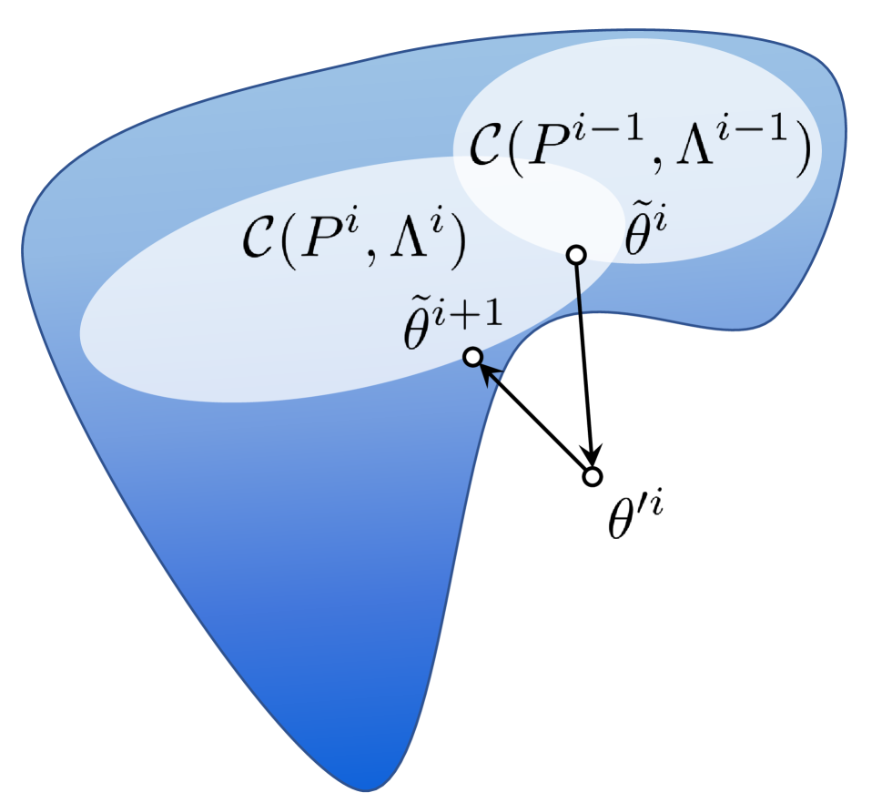
Figure 5: Illustration of Algorithm 1. The set of all the stabilizing $\tilde{\theta}$ is given in blue.

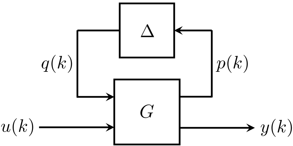
(a) uncertain plant $F_{u}(G,\Delta)$

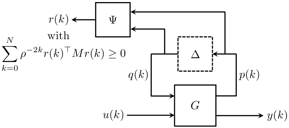
(b) extended system of $G$ and $\Psi$ with IQCs

Figure 6: Uncertain plant and its corresponding constrained extended system

Projected Policy Gradient

Policy gradient methods (Sutton et al. 1999; Williams 1992) enjoy convergence to optimality under the tabular setting and achieve good empirical performance for more challenging problems. However, with little assumption about the problem setting, they do not offer any stability guarantee for the closed loop system. We propose the projected policy gradient method that enforces the stability of the interconnected system while the policy is dynamically explored and updated.

Policy gradient approximates the gradient with respect to the parameters of a stochastic controller using samples of trajectories via (18) without any prior knowledge of plant parameters and the reward structures. Gradient ascent is then applied to refine the controller with the estimated gradients.

$$\nabla_{\tilde{\theta}}R(\pi_{\tilde{\theta}}) =\int_{\mathcal{X}}d^{\pi_{\tilde{\theta}}}(x)\int_{\mathcal{U}}\nabla_{\tilde{\theta}}\pi_{\tilde{\theta}}(u|x)Q^{\pi_{\tilde{\theta}}}(x,u)dudx$$

$$=\mathbb{E}_{\tilde{\theta},x\sim d^{\pi},u\sim\pi_{\tilde{\theta}}}[Q^{\pi}(x,u)\nabla_{\tilde{\theta}}\log\pi_{\tilde{\theta}}(u|x)].$$ (18)

In the above, $\tilde{\theta}$ represents the parameters of $\pi_{\tilde{\theta}}$. $R(\pi_{\tilde{\theta}})$ is the expected reward (negative cost) of the controller $\pi_{\tilde{\theta}}$. $d^{\pi}(x)$ is the distribution of states $x\in\mathcal{X}$ under $\pi_{\tilde{\theta}}$, where $\mathcal{X}$ is a set of states. $Q^{\pi}(x,u)$ is the reward-to-go after executing control $u\in\mathcal{U}$ at state $x$ under $\pi_{\tilde{\theta}}$, where $\mathcal{U}$ is a set of actions.

Like any gradient method, policy gradient does not ensure the controller is in some specific set of preference (the set of stabilizing controller in our setting). To that end, a projection to the stability set $\mathcal{C}(\bar{P},\bar{\Lambda})$, $(Q_{1},Q_{2},\tilde{\theta})\leftarrow\Pi_{\mathcal{C}(\bar{P},\bar{\Lambda})}(\theta^{\prime})$, is applied between gradient updates, where $\theta^{\prime}$ is the updated parameter, and the projection operator $\Pi_{\mathcal{C}(\bar{P},\bar{\Lambda})}(\theta^{\prime})$ is defined as the following convex program,

$$\Pi_{\mathcal{C}(\bar{P},\bar{\Lambda})}(\theta^{\prime})\in\arg\min_{\begin{subarray}{c}Q_{1},Q_{2},\tilde{\theta}\end{subarray}} \;\;{\left\|\begin{bmatrix}Q_{1}\\ Q_{2}\end{bmatrix}-\begin{bmatrix}\bar{P}^{-1}\\ \bar{\Lambda}^{-1}\end{bmatrix}\right\|_{F}^{2}+\|\tilde{\theta}-\theta^{\prime}\|_{F}^{2}}$$

s.t. $$\;\;\text{LMI}(Q_{1},Q_{2},\tilde{\theta},\bar{P},\bar{\Lambda}).$$ (19)

Through the recursively feasible projection step (i.e. the feasibility is inherited in subsequent steps, summarized in Theorem A.1 in Appendix A), we conclude with a projected policy gradient method to synthesize stabilizing RNN controllers as summarized in Algorithm 1 and illustrated in Fig. 5.

Algorithm 1 Projected Policy Gradient

1:Matrices $P^{0}$ and $\Lambda^{0}$ s.t. $\mathcal{C}(P^{0},\Lambda^{0})$ is not empty, learning rate $\sigma>0$.

2:$i\leftarrow 0$

3:while not converged do

4:     $\theta^{\prime i}\leftarrow\tilde{\theta}^{i}+\sigma\nabla_{\tilde{\theta}}R(\pi_{\tilde{\theta}^{i}})$ $\triangleright$ gradient step

5:     $(Q_{1}^{i+1},Q_{2}^{i+1},\tilde{\theta}^{i+1})\leftarrow\Pi_{\mathcal{C}(P^{i},\Lambda^{i})}(\theta^{\prime i})$ $\triangleright$ proj. step

6:     $P^{i+1}\leftarrow(Q_{1}^{i+1})^{-1}$,  $\Lambda^{i+1}\leftarrow(Q_{2}^{i+1})^{-1}$

7:     $i\leftarrow i+1$

8:end while

9:$\pi_{\tilde{\theta}}$

In the algorithm, the gradient step performs gradient ascent using the estimated gradient $\nabla_{\tilde{\theta}}R(\pi(\tilde{\theta}))$. The projection step projects the updated parameters $\theta^{\prime i}$ from the gradient step to the convex stability set $\mathcal{C}(P^{i},\Lambda^{i})$, where $P^{i}$ and $\Lambda^{i}$ are computed using $Q_{1}^{i}$ and $Q_{2}^{i}$ from the previous projection step. We choose $\Lambda^{0}=I_{n_{\phi}}$, and construct $P^{0}$ based on the method in (Scherer, Gahinet, and Chilali 1997).

Remark 3.3.

The projection step (19) is a semi-definite program (SDP) involving $O((n_{\xi}+n_{\phi})\times(n_{\xi}+n_{\phi}))$ variables. The complexity of interior point SDP solvers usually scales cubically with the number of variables, potentially bringing computational burden when $(n_{\xi}+n_{\phi})$ is large. Luckily, most high dimensional problems admit low dimension structures (Wright and Ma 2021) and such overhead is only paid at training without further operations at deployment.

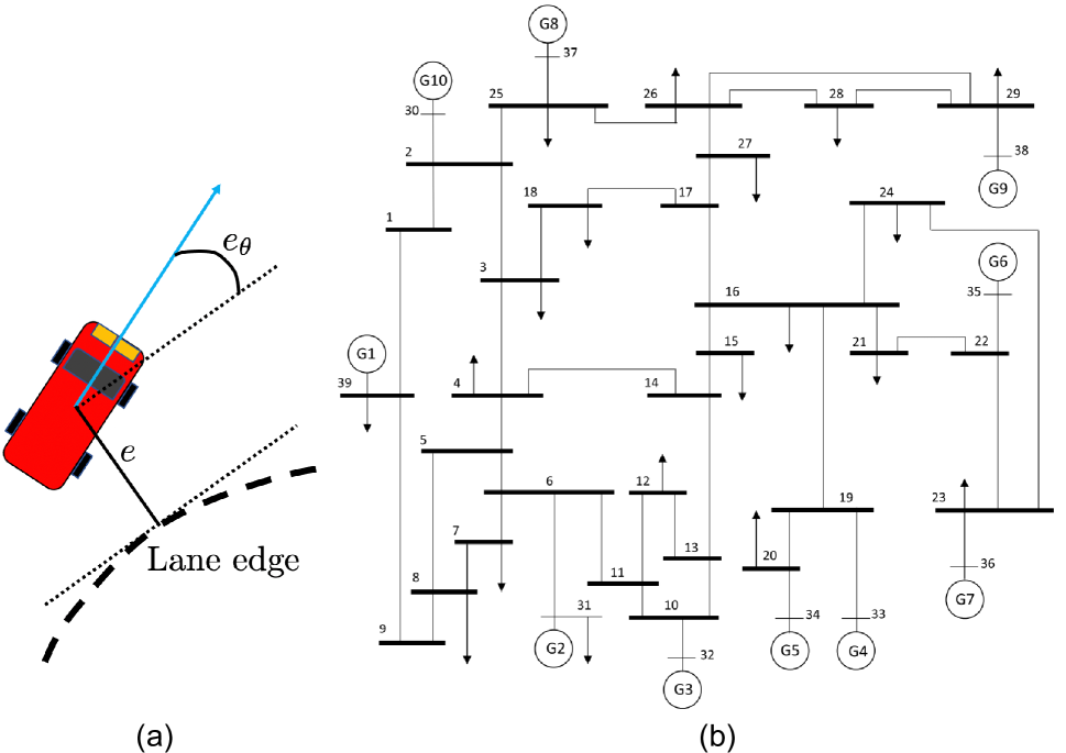
Figure 7: (a) Vehicle (Alleyne 1997); (b) Frequency Regulation on IEEE 39-bus New England Power System (Athay, Podmore, and Virmani 1979)

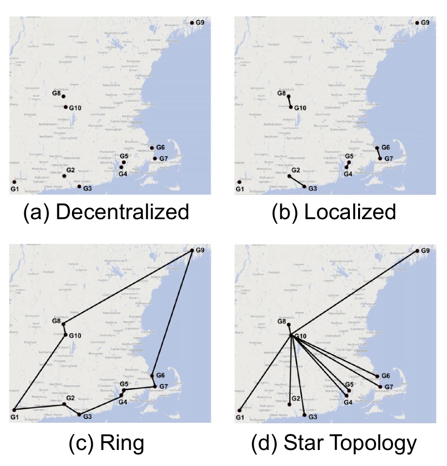
Figure 8: Four communication topologies for IEEE 39-bus power system (Fazelnia et al. 2016).

4 Partially Observed Nonlinear Systems with Uncertainty

In the context of RL, we often need to handle systems with nonlinear dynamics and/or unmodeled dynamics. Here we model such a nonlinear and uncertain plant $F_{u}(G,\Delta)$ (shown in Fig. 6(a)) as an interconnection of the nominal plant $G$, and the perturbation $\Delta$ representing the nonlinear, and uncertain part of the system. Therefore, in this new problem setting, we only require system dynamics to be partially known, and we use $\Delta$ to cover the difference between the original real system dynamics, and partially known dynamics $G$. The plant $F_{u}(G,\Delta)$ is defined by the following equations:

$$G\left\{\begin{array}[]{ll}x(k+1)&=A_{G}\ \ x(k)+B_{G1}\ q(k)+B_{G2}\ u(k)\\ p(k)&=C_{G1}\ x(k)+D_{G1}\ q(k)\\ y(k)&=C_{G2}\ x(k)\end{array}\right.$$ (23)

$$\hskip 22.76228ptq(\cdot)\hskip 26.17648pt=\Delta(p(\cdot))$$ (24)

where $x(k)\in\mathbb{R}^{n_{G}}$, $u(k)\in\mathbb{R}^{n_{u}}$, and $y(k)\in\mathbb{R}^{n_{y}}$ are the state, control input, and output of the nominal plant $G$, and $p(k)$ and $q(k)$ are the input and output of $\Delta$. The perturbation $\Delta:\ell_{2e}^{n_{p}}\rightarrow\ell_{2e}^{n_{q}}$ is a causal and bounded operator.

The perturbation $\Delta$ can represent various types of uncertainties and nonlinearities, including sector bounded nonlinearities, slope restricted nonlinearities, and unmodeled dynamics. Thus considering $\Delta$ extends our framework to the class of plants beyond LTI plants. The input-output relationship of $\Delta$ is characterized with an integral quadratic constraint (IQC) (Megretski and Rantzer 1997), which consists of a filter $\Psi$ applied to the input $p$ and output $q$ of $\Delta$, and a constraint on the output $r$ of $\Psi$. The filter $\Psi$ is an LTI system with the zero initial condition $\psi(0)=0_{n_{\psi\times 1}}$:

$$\begin{array}[]{ll}\psi(k+1)&=A_{\psi}\ \psi(k)+B_{\psi 1}\ p(k)+B_{\psi 2}\ q(k),\\ r(k)&=C_{\psi}\ \psi(k)+D_{\psi 1}\ p(k)+D_{\psi 2}\ q(k).\end{array}$$ (25c)

To enforce exponential stability of the feedback system, we characterize $\Delta$ using the time-domain $\rho$-hard IQC, which is introduced in (Lessard, Recht, and Packard 2016), and its definition is also provided below.

Definition 4.1.

Let $\Psi$ be an LTI system defined in (25), and $M\in\mathbb{S}^{n_{r}}$. Suppose $0\leq\rho\leq 1$. A bounded, causal operator $\Delta:\ell_{2e}^{n_{p}}\rightarrow\ell_{2e}^{n_{q}}$ satisfies the time-domain $\rho$-hard IQC defined by $\Psi$, $M$, and $\rho$, if the following condition holds for all $p\in\ell_{2e}^{n_{p}}$, $q=\Delta(p)$, and $N\geq 0$

$$\sum_{k=0}^{N}\rho^{-2k}r(k)^{\top}Mr(k)\geq 0.$$ (26)

where $r$ is the output of $\Psi$ driven by inputs $(p,q)$.

Remark 4.1.

For a particular perturbation $\Delta$, there is typically a class of valid $\rho$-hard IQCs defined by a fixed filter $\Psi$ and a matrix $M$ drawn from a convex set $\mathcal{M}$. Thus, in the stability condition derived later, $M\in\mathcal{M}$ will also be treated as a decision variable. A library of frequency-domain $\rho$-IQCs is provided in (Boczar et al. 2017) for various types of perturbations. As shown in (Schwenkel et al. 2021), a general class of frequency-domain $\rho$-IQCs can be translated into time-domain $\rho$-hard IQC by a multiplier factorization.

When deriving the stability condition, the perturbation $\Delta$ will be replaced by the time-domain $\rho$-hard IQC (26) that describes it, and the associated filter $\Psi$, as shown in Fig. 6(b). Therefore, the stabilizing controller will be designed for the extended system (an interconnection of $G$ and $\Psi$) subject to IQCs, instead of the original $F_{u}(G,\Delta)$. This controller will also be able to stabilize the original $F_{u}(G,\Delta)$. Define the extended state as $x_{e}=[x^{\top},\ \psi^{\top}]^{\top}$, and the dynamics of the extended system are given in Appendix A. Define $\zeta=[x_{e}^{\top},\ \ \xi^{\top}]^{\top}$ to gather the states of the extended system and the controller. The feedback system of the extended system and the controller has the dynamics

$$\begin{array}[]{ll}\zeta(k+1)&=\mathcal{A}\ \zeta(k)+\mathcal{B}_{1}\ q(k)+\ \mathcal{B}_{2}\ z(k),\\ v(k)&=\mathcal{C}_{1}\ \zeta(k)+\mathcal{D}_{1}\ q(k)+\mathcal{D}_{2}\ z(k),\\ r(k)&=\mathcal{C}_{2}\ \zeta(k)+\mathcal{D}_{3}\ q(k)+\mathcal{D}_{4}\ z(k),\end{array}$$ (30)

where

$$\begin{array}[]{ll}&\hskip 3.69899pt\mathcal{A}=\left[\begin{smallmatrix}A_{e}+B_{e2}\tilde{D}_{k2}C_{e2}&B_{e2}\tilde{C}_{k1}\\ \tilde{B}_{k2}C_{e2}&\tilde{A}_{k}\end{smallmatrix}\right],\hskip 24.18501pt\mathcal{B}_{1}=\left[\begin{smallmatrix}B_{e1}\\ 0_{n_{\xi}\times n_{q}}\end{smallmatrix}\right],\\ &\hskip 0.85355pt\mathcal{B}_{2}=\left[\begin{smallmatrix}B_{e2}D_{k1}\frac{B_{\phi}-A_{\phi}}{2}\\ B_{k1}\frac{B_{\phi}-A_{\phi}}{2}\end{smallmatrix}\right],\hskip 52.63777pt\mathcal{C}_{1}=\left[\begin{smallmatrix}D_{k3}C_{e2}&C_{k2}\end{smallmatrix}\right],\\ &\mathcal{D}_{1}=0_{n_{\phi}\times n_{q}},\hskip 18.49411pt\mathcal{D}_{2}=0_{n_{\phi}\times n_{\phi}},\hskip 17.07182pt\mathcal{C}_{2}=\left[\begin{smallmatrix}C_{e1}&0_{n_{r}\times n_{\xi}}\end{smallmatrix}\right],\\ &\mathcal{D}_{3}=D_{e1},\hskip 32.15175pt\mathcal{D}_{4}=0_{n_{r}\times n_{\phi}},\end{array}$$

and the state space matrices $(A_{e},B_{e1},...,D_{e1})$ of the extended system are defined in Appendix A. The next theorem merges the QC for $\tilde{\phi}$ and the time-domain $\rho$-hard IQC for $\Delta$ with the Lyapunov theorem to derive the exponential stability condition for the uncertain feedback system.

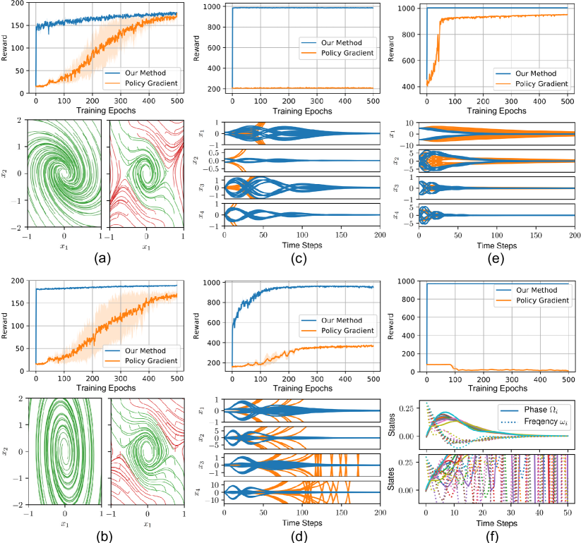
Figure 9: (a) Inverted Pendulum (linear); (b) Inverted Pendulum (nonlinear); (c) Cartpole; (d) Pendubot; (e) Vehicle lateral control; (f) IEEE 39-bus New England Power System frequency regulation. The error bars of reward plots characterize standard deviation across 3 runs with different seeds. For (a) and (b), the left figures are from our method and right figures from policy gradient. Converging trajectories are rendered in green while diverging ones in red. For (c), (d), (e), trajectories from our method are given in blue while those from policy gradient are in orange. For (f), top figure is given by our method and bottom one by policy gradient.

Theorem 4.1.

Consider the feedback system of uncertain plant $F_{u}(G,\Delta)$, and RNN controller $\pi_{\tilde{\theta}}$. Assume $\Delta$ satisfies the time-domain $\rho$-hard IQC defined by $\Psi$, $\mathcal{M}$, and $\rho$, with $0\leq\rho\leq 1$. Given $\bar{P}\in\mathbb{R}^{n_{\zeta}\times n_{\zeta}}$ and $\bar{\Lambda}\in\mathbb{R}^{n_{\phi}\times n_{\phi}}$. If there exist matrices $Q_{1}\in\mathbb{S}_{++}^{n_{\zeta}}$, $Q_{2}\in\mathbb{D}_{++}^{n_{\phi}}$, $M\in\mathcal{M}$, and parameters $\tilde{\theta}$ such that the following condition holds

$$\begin{bmatrix}R^{\top}\Gamma R~{}~{}~{}~{}~{}~{}~{}~{}~{}&\begin{bmatrix}\mathcal{A}&\mathcal{B}_{1}&\mathcal{B}_{2}\\ \mathcal{C}_{1}&\mathcal{D}_{1}&\mathcal{D}_{2}\end{bmatrix}^{\top}\\ \begin{bmatrix}\mathcal{A}&\mathcal{B}_{1}&\mathcal{B}_{2}\\ \mathcal{C}_{1}&\mathcal{D}_{1}&\mathcal{D}_{2}\end{bmatrix}&\begin{bmatrix}Q_{1}&0\\ 0&Q_{2}\end{bmatrix}\end{bmatrix}\succeq 0,$$ (33)

where $\Gamma=\mathop{\bf diag}(\rho^{2}(2\bar{P}-\bar{P}^{\top}Q_{1}\bar{P}),2\bar{\Lambda}-\bar{\Lambda}^{\top}Q_{2}\bar{\Lambda},-M)$ is a block diagonal matrix and $R=\left[\begin{smallmatrix}I&0&0\\ 0&0&I\\ \mathcal{C}_{2}&\mathcal{D}_{3}&\mathcal{D}_{4}\end{smallmatrix}\right]$. Then for any $x(0)$, we have $\|x(k)\|\leq\sqrt{\text{cond}(P)}\rho^{k}\|x(0)\|$ for all $k$, where $P:=Q_{1}^{-1}$, i.e., the feedback system is exponentially stable with rate $\rho$.

The complete proof is provided in Appendix A. This LMI (33) is jointly convex in $\tilde{\theta},Q_{1},Q_{2}$ and $M$ for any given $\bar{P}$ and $\bar{\Lambda}$. Based on this LMI, we define the convex robust stability set $\mathcal{C}_{R}(\bar{P},\bar{\Lambda})$:

$$\mathcal{C}_{R}(\bar{P},\bar{\Lambda}):=\left\{\tilde{\theta}:\ \exists\ Q_{1}\in\mathbb{S}_{++}^{n_{\zeta}},\ Q_{2}\in\mathbb{D}_{++}^{n_{\phi}},\ M\in\mathcal{M},\ \text{s.t.}\ \eqref{eq:convex_robust_stab}\right\}.$$

Any parameter $\tilde{\theta}$ drawn from $\mathcal{C}_{R}(\bar{P},\bar{\Lambda})$ ensures the exponential stability of the feedback system of $F_{u}(G,\Delta)$ and $\pi_{\tilde{\theta}}$, and this convex robust stability set can be used in the projection step.

Remark 4.2.

If we only require the feedback system to be stable ($\rho=1$ in (33)), a more general class of IQCs, the time-domain hard IQCs (Megretski and Rantzer 1997), can be used to describe $\Delta$.

5 Numerical Experiment

To compare our method against regular RNN controller trained without projection, we consider 6 different tasks involving control of partially observed dynamical systems, including a linearized inverted pendulum and its nonlinear variant, a cartpole, vehicle lateral dynamics, a pendubot, and a high dimensional power system. Fig. 8 gives a demonstrative visualization of tasks including vehicle lateral control and IEEE 39-bus power system frequency regulation, whose communication topologies are shown in Fig. 8. Experimental settings and tasks definitions are detailed in Appendix B.

The experimental results including rewards and sample trajectories at convergence are reported in Fig. 9. In all experiments, our method achieves high reward after the first few projection steps that ensures stability, greatly outperforming the regular method which suffers from instability even after converging. For pendubot and inverted pendulum tasks, our method keeps perfecting the performance after the first projection steps which already give high performance. While for cartpole, vehicle lateral control, and power system frequency regulation tasks, our method converges to optimal performance in one step. Our method gives converging trajectories for all tasks and achieves faster converging trajectories on the vehicle lateral control task. In comparison, policy gradient has been greatly impacted by the partial observability and converges to sub-optimal performance in cartpole, pendubot, and power system frequency regulation tasks and requires more steps to achieve optimal performance in inverted pendulum and vehicle lateral control tasks. Without stability guarantee, policy gradient fails to ensure converging trajectories from some initial conditions for all tasks excluding vehicle lateral control which is open-loop stable.

6 Conclusion

In this work, we present a method to synthesize stabilizing RNN controllers, which ensures the stability of the feedback systems both during learning and control process. We develop a convex set of stabilizing RNN parameters for nonlinear and partially observed systems. A novel projected policy gradient method is developed to synthesize a controller while enforcing stability by recursively projecting the parameters of the RNN controller to the convex set. By evaluating on a variety of control tasks, we demonstrate that our method learns stabilizing controllers with fewer samples, faster converging trajectories, and higher final performance than policy gradient. Future directions include extensions to implicit models (Bai, Kolter, and Koltun 2019; El Ghaoui et al. 2020), and model-free RL (Jiang and Jiang 2012).

Supplementary material

Appendix A Proofs and Illustrations

Derivation for the Transformed Plant $\tilde{P}_{\pi}$

The input to $P_{\pi}$ is transformed by the following equation:

$$w(k)=\frac{B_{\phi}-A_{\phi}}{2}z(k)+\frac{A_{\phi}+B_{\phi}}{2}v(k).$$ (34)

Substituting the expression of $v(k)$ from (6) into (34) yields

$$w(k)=\frac{B_{\phi}-A_{\phi}}{2}z(k)+\frac{A_{\phi}+B_{\phi}}{2}C_{K2}\ \xi(k)+\frac{A_{\phi}+B_{\phi}}{2}D_{K3}\ y(k).$$ (35)

Finally, the transformed plant $\tilde{P}_{\pi}$ can be obtained by substituting (35) into (6).

Proof of Theorem 3.1

Proof.

Assume there exist $Q_{1}\in\mathbb{S}_{++}^{n_{\zeta}}$, $Q_{2}\in\mathbb{D}_{++}^{n_{\phi}}$, and $\tilde{\theta}$, such that (16) holds. It follows from Schur complements that (16) is equivalent to

$$\begin{bmatrix}\mathcal{A}&\mathcal{B}\\ \mathcal{C}&\mathcal{D}\end{bmatrix}^{\top}\begin{bmatrix}Q_{1}^{-1}&0\\ 0&Q_{2}^{-1}\end{bmatrix}\begin{bmatrix}\mathcal{A}&\mathcal{B}\\ \mathcal{C}&\mathcal{D}\end{bmatrix}-\begin{bmatrix}\rho^{2}(2\bar{P}-\bar{P}^{\top}Q_{1}\bar{P})&0\\ 0&2\bar{\Lambda}-\bar{\Lambda}^{\top}Q_{2}\bar{\Lambda}\end{bmatrix}\preceq 0.$$ (36)

It follows from the inequalities $\bar{P}^{\top}Q_{1}\bar{P}-2\bar{P}\succeq-Q_{1}^{-1}$ and $\bar{\Lambda}^{\top}Q_{2}\bar{\Lambda}-2\bar{\Lambda}\succeq-Q_{2}^{-1}$ for any $\bar{P}\in\mathbb{R}^{n_{\zeta}\times n_{\zeta}}$ and $\bar{\Lambda}\in\mathbb{R}^{n_{\phi}\times n_{\phi}}$ (Tobenkin, Manchester, and Megretski 2017; Revay, Wang, and Manchester 2020) that (36) implies

$$\begin{bmatrix}\mathcal{A}&\mathcal{B}\\ \mathcal{C}&\mathcal{D}\end{bmatrix}^{\top}\begin{bmatrix}Q_{1}^{-1}&0\\ 0&Q_{2}^{-1}\end{bmatrix}\begin{bmatrix}\mathcal{A}&\mathcal{B}\\ \mathcal{C}&\mathcal{D}\end{bmatrix}-\begin{bmatrix}\rho^{2}Q_{1}^{-1}&0\\ 0&Q_{2}^{-1}\end{bmatrix}\preceq 0.$$ (37)

Defining $P=Q_{1}^{-1}$, and $\Lambda=Q_{2}^{-1}$, and rearranging (37), we have that $P,\Lambda$, and $\tilde{\theta}$ satisfy the following condition

$$\begin{bmatrix}\mathcal{A}^{\top}P\mathcal{A}-\rho^{2}P&\mathcal{A}^{\top}P\mathcal{B}\\ \mathcal{B}^{\top}P\mathcal{A}&\mathcal{B}^{\top}P\mathcal{B}\end{bmatrix}+\begin{bmatrix}\mathcal{C}&\mathcal{D}\\ 0&I\end{bmatrix}^{\top}\begin{bmatrix}\Lambda&0\\ 0&-\Lambda\end{bmatrix}\begin{bmatrix}\mathcal{C}&\mathcal{D}\\ 0&I\end{bmatrix}\preceq 0,$$ (38)

Define the Lyapunov function $V(\zeta):=\zeta^{\top}P\zeta$. Multiplying (38) on the left and right by $[\zeta(k)^{\top},\ z(k)^{\top}]$ and its transpose yields

$$V(\zeta(k+1))-\rho^{2}V(\zeta(k))+\begin{bmatrix}v(k)\\ z(k)\end{bmatrix}^{\top}\begin{bmatrix}\Lambda&0\\ 0&-\Lambda\end{bmatrix}\begin{bmatrix}v(k)\\ z(k)\end{bmatrix}\leq 0.$$ (39)

It follows from $\tilde{\phi}\in$ sector $[-1_{n_{\phi}\times 1},1_{n_{\phi}\times 1}]$ that the last term in (39) is nonnegative, and thus $V(\zeta(k+1))\leq\rho^{2}V(\zeta(k))$. Iterate it down to $k=0$, we have $V(\zeta(k))\leq\rho^{2k}V(\zeta(0))$, which implies $\|\zeta(k)\|\leq\sqrt{\text{cond}(P)}\rho^{k}\|\zeta(0)\|$. Recall $\xi(0)=0$. Therefore

$$\|x(k)\|\leq\|\zeta(k)\|\leq\sqrt{\text{cond}(P)}\rho^{k}\|\zeta(0)\|=\sqrt{\text{cond}(P)}\rho^{k}\|x(0)\|,$$

and this completes the proof.    

Recursive Feasibility of the Projection Steps

Theorem A.1 (Recursive Feasibility).

If LMI$(Q_{1},Q_{2},\tilde{\theta},P^{i-1},\Lambda^{i-1})$ is feasible (i.e.  LMI$(Q_{1},Q_{2},\tilde{\theta},P^{i-1},\Lambda^{i-1})$ holds for some $Q_{1}$, $Q_{2}$, and $\tilde{\theta}$), then LMI$(Q_{1},Q_{2},\tilde{\theta},P^{i},\Lambda^{i})$ is also feasible, where $P^{i}=(Q_{1}^{i})^{-1}$ and $\Lambda^{i}=(Q_{2}^{i})^{-1}$ are from the $i$-th step of projected policy gradient, for $i=1,2,\ldots$

Proof.

The main idea is to show that $(Q_{1}^{i},Q_{2}^{i},\tilde{\theta}^{i})$ is already a feasible point for LMI$(Q_{1},Q_{2},\tilde{\theta},P^{i},\Lambda^{i})$. Since LMI$(Q_{1},Q_{2},\tilde{\theta},P^{i-1},\Lambda^{i-1})$ is feasible, at optimum of the projection step, we obtain the minimizer $(Q_{1}^{i},Q_{2}^{i},\tilde{\theta}^{i})$ and LMI$(Q_{1}^{i},Q_{2}^{i},\tilde{\theta}^{i},P^{i-1},\Lambda^{i-1})$ holds. It follows from inequalities $2P^{i-1}-P^{i-1}{}^{\top}Q_{1}^{i}P^{i-1}\preceq(Q_{1}^{i})^{-1}$ and $2\Lambda^{i-1}-\Lambda^{i-1}{}^{\top}Q_{2}^{i}\Lambda^{i-1}\preceq(Q_{2}^{i})^{-1}$ that

$$\begin{bmatrix}\rho^{2}(Q_{1}^{i})^{-1}&0&\mathcal{A}^{\top}&\mathcal{C}^{\top}\\ 0&(Q_{2}^{i})^{-1}&\mathcal{B}^{\top}&\mathcal{D}^{\top}\\ \mathcal{A}&\mathcal{B}&Q_{1}^{i}&0\\ \mathcal{C}&\mathcal{D}&0&Q_{2}^{i}\end{bmatrix}\succeq 0,$$ (40)

which renders LMI$(Q_{1}^{i},Q_{2}^{i},\tilde{\theta}^{i},P^{i},\Lambda^{i})$ true at a feasible point of $(Q_{1}^{i},Q_{2}^{i},\tilde{\theta}^{i})$.    

Dynamics of the Extended System

The extended system (shwon in Fig. 6(b)) is of the form

$$x_{e}(k+1) =A_{e}\ x_{e}(k)+B_{e1}\ q(k)+B_{e2}\ u(k)$$ (41a)

$$r(k) =C_{e1}\ x_{e}(k)+D_{e1}\ q(k)$$ (41b)

$$y(k) =C_{e2}\ x_{e}(k)$$ (41c)

where

$$A_{e} =\begin{bmatrix}A_{G}&0\\ B_{\psi 1}C_{G1}&A_{\psi}\end{bmatrix},\ B_{e1}=\begin{bmatrix}B_{G1}\\ B_{\psi 1}D_{G1}+B_{\psi 2}\end{bmatrix},\ B_{e2}=\begin{bmatrix}B_{G2}\\ 0\end{bmatrix}$$

$$C_{e1} =\begin{bmatrix}D_{\psi 1}C_{G1}&C_{\psi}\end{bmatrix},\ \ \ D_{e1}=\begin{bmatrix}D_{\psi 1}D_{G1}+D_{\psi 2}\end{bmatrix},\ \ C_{e2}=\begin{bmatrix}C_{G2}&0\end{bmatrix}.$$ (42a)

Proof of Theorem 4.1

Proof.

Assume there exist $Q_{1}\in\mathbb{S}_{++}^{n_{\zeta}}$, $Q_{2}\in\mathbb{D}_{++}^{n_{\phi}}$, $M\in\mathcal{M}$, and $\tilde{\theta}$ such that (33) holds. It follows from Schur complements that (33) is equivalent to

$${\begin{bmatrix}\mathcal{A}&\mathcal{B}_{1}&\mathcal{B}_{2}\\ \mathcal{C}_{1}&\mathcal{D}_{1}&\mathcal{D}_{2}\end{bmatrix}^{\top}\begin{bmatrix}Q_{1}^{-1}&0\\ 0&Q_{2}^{-1}\end{bmatrix}\begin{bmatrix}\mathcal{A}&\mathcal{B}_{1}&\mathcal{B}_{2}\\ \mathcal{C}_{1}&\mathcal{D}_{1}&\mathcal{D}_{2}\end{bmatrix}-R^{\top}\begin{bmatrix}\rho^{2}(2\bar{P}-\bar{P}^{\top}Q_{1}\bar{P})&0&0\\ 0&2\bar{\Lambda}-\bar{\Lambda}^{\top}Q_{2}\bar{\Lambda}&0\\ 0&0&-M\end{bmatrix}R}\preceq 0.$$ (43)

By inequalities $\bar{P}^{\top}Q_{1}\bar{P}-2\bar{P}\succeq-Q_{1}^{-1}$ and $\bar{\Lambda}^{\top}Q_{2}\bar{\Lambda}-2\bar{\Lambda}\succeq-Q_{2}^{-1}$ for any $\bar{P}\in\mathbb{R}^{n_{\zeta}\times n_{\zeta}}$ and $\bar{\Lambda}\in\mathbb{R}^{n_{\phi}\times n_{\phi}}$, we have that (43) implies

$$\begin{bmatrix}\mathcal{A}&\mathcal{B}_{1}&\mathcal{B}_{2}\\ \mathcal{C}_{1}&\mathcal{D}_{1}&\mathcal{D}_{2}\end{bmatrix}^{\top}\begin{bmatrix}Q_{1}^{-1}&0\\ 0&Q_{2}^{-1}\end{bmatrix}\begin{bmatrix}\mathcal{A}&\mathcal{B}_{1}&\mathcal{B}_{2}\\ \mathcal{C}_{1}&\mathcal{D}_{1}&\mathcal{D}_{2}\end{bmatrix}-R^{\top}\begin{bmatrix}\rho^{2}Q_{1}^{-1}&0&0\\ 0&Q_{2}^{-1}&0\\ 0&0&-M\end{bmatrix}R\preceq 0.$$ (44)

Defining $P=Q_{1}^{-1}$ and $\Lambda=Q_{2}^{-1}$, and rearranging (44), we have $P,\Lambda,M$, and $\tilde{\theta}$ satisfy the following condition

$$\begin{bmatrix}\mathcal{A}&\mathcal{B}_{1}&\mathcal{B}_{2}\\ I&0&0\end{bmatrix}^{\top}\begin{bmatrix}P&0\\ 0&-\rho^{2}P\end{bmatrix}\begin{bmatrix}\mathcal{A}&\mathcal{B}_{1}&\mathcal{B}_{2}\\ I&0&0\end{bmatrix}+\begin{bmatrix}\mathcal{C}_{1}&\mathcal{D}_{1}&\mathcal{D}_{2}\\ 0&0&I\end{bmatrix}^{\top}\begin{bmatrix}\Lambda&0\\ 0&-\Lambda\end{bmatrix}\begin{bmatrix}\mathcal{C}_{1}&\mathcal{D}_{1}&\mathcal{D}_{2}\\ 0&0&I\end{bmatrix}$$

$$\hskip 17.07182pt+\begin{bmatrix}\mathcal{C}_{2}&\mathcal{D}_{3}&\mathcal{D}_{4}\end{bmatrix}^{\top}M\begin{bmatrix}\mathcal{C}_{2}&\mathcal{D}_{3}&\mathcal{D}_{4}\end{bmatrix}\preceq 0.$$ (45)

Define the Lyapunov function $V(\zeta):=\zeta^{\top}P\zeta$. Multiplying (A) on the left and right by $\begin{bmatrix}\zeta(k)^{\top},\ q(k)^{\top},\ z(k)^{\top}\end{bmatrix}$ and its transpose yields

$$V(\zeta(k+1))-\rho^{2}V(\zeta(k))+\begin{bmatrix}v(k)\\ z(k)\end{bmatrix}^{\top}\begin{bmatrix}\Lambda&0\\ 0&-\Lambda\end{bmatrix}\begin{bmatrix}v(k)\\ z(k)\end{bmatrix}+r(k)^{\top}Mr(k)\leq 0.$$ (46)

It follows from $\tilde{\phi}\in$ sector $[-1_{n_{\phi}\times 1},1_{n_{\phi}\times 1}]$ that the third term is nonnegative. This yields

$$V(\zeta(k+1))-\rho^{2}V(\zeta(k))+r(k)^{\top}Mr(k)\leq 0..$$ (47)

Multiply (47) by $\rho^{-2k}$ for each $k$ and sum over $k$ to obtain

$$\rho^{-2(k-1)}V(\zeta(k))-\rho^{2}V(\zeta(0))+\sum_{t=0}^{k-1}\rho^{-2t}r(t)Mr(t)\leq 0.$$ (48)

By the assumption that $\Delta$ satisfies the $\rho$-hard IQC, the last term is nonnegative, and thus $V(\zeta(k))\leq\rho^{2k}V(\zeta(0))$ for all $k$, which implies $\|\zeta(k)\|\leq\sqrt{\text{cond}(P)}\rho^{k}\|\zeta(0)\|$. Recall $\xi(0)=0_{n_{\xi}\times 1}$ and $\psi(0)=0_{n_{\psi}\times 1}$. Therefore

$$\|x(k)\|\leq\|\zeta(k)\|\leq\sqrt{\text{cond}(P)}\rho^{k}\|\zeta(0)\|=\sqrt{\text{cond}(P)}\rho^{k}\|x(0)\|,$$

and this completes the proof.    

Appendix B More on Experiments

In this section, we give detailed information about the experiments. All experiments are conducted on a custom built machine with 36-core Intel Broadwell Xeon CPUs with 64 GB of RAM and are terminated in tens of minutes. In all tasks, both our method and policy gradient are trained to convergence and are capped at 1000 epochs. For each epoch, the gradient is estimated from a batch of 6000 step data sampled from the controller interacting with the plant and is applied to update the parameters. The trajectory length is capped at $200$. The average reward from the sample of trajectories from the 6000 steps are reported. We show 500 epoch plots in Fig. 9 for clearer capture of the convergence process. The experiments and models are coded in Python (Van Rossum and Drake 2009) with Tensorflow (Abadi et al. 2015), CVXPY (Diamond and Boyd 2016) and MOSEK. We choose the learning rate of 1e-3, picked from grid search from 1e-1, 1e-2, 1e-3, 1e-4 to give best reward at convergence for policy gradient on the inverted pendulum task. We use ADAM optimizer (Kingma and Ba 2014) and gradient clipping to a maximum magnitude of $10$ for each parameter. We use $\tanh$ activation for all our neural network controllers. The implementation of policy gradient is consistent with Levine (2021). And our method adds the projection updates on the same code base. The initial guess for the Lyapunov matrix $P^{0}$ of Algorithm 1 is constructed using the method introduced in (Scherer, Gahinet, and Chilali 1997), which computes the Lyapunov matrix for output feedback control problem through LMIs. The initial guess for $\Lambda^{0}$ is an identity matrix.

Inverted Pendulum

We consider both a linearized inverted pendulum system and a full nonlinear version whose dynamics are given below. Both examples have two states $x_{1}$, $x_{2}$, representing the angular position (rad) and velocity (rad/s). Only the plant output, $y=x_{1}$, is observed. Our methods as described in Section 3 and 4 are applied for the linear, and nonlinear variants, with the goal of balancing the inverted pendulum around the upright position.

Consider an inverted pendulum with mass $m=0.15$ kg, length $l=0.5$ m, and friction coefficient $\mu=0.5$ Nms$/$rad. The discretized and linearized dynamics are:

$$\begin{bmatrix}x_{1}(k+1)\\ x_{2}(k+1)\end{bmatrix} =\begin{bmatrix}1&\delta\\ \frac{g\delta}{l}&1-\frac{\mu\delta}{ml^{2}}\end{bmatrix}\begin{bmatrix}x_{1}(k)\\ x_{2}(k)\end{bmatrix}+\begin{bmatrix}0\\ \frac{\delta}{ml^{2}}\end{bmatrix}u(k),$$

$$y(k) =\begin{bmatrix}1&0\end{bmatrix}\begin{bmatrix}x_{1}(k)\\ x_{2}(k)\end{bmatrix},$$ (49)

where $u$ is the control input (1/10 Nm), and $\delta=0.02$ s is the sampling time.

The discretized nonlinear dynamics of the inverted pendulum are

$$\begin{bmatrix}x_{1}(k+1)\\ x_{2}(k+1)\end{bmatrix} =\begin{bmatrix}1&\delta\\ \frac{g\delta}{l}&1-\frac{\mu\delta}{ml^{2}}\end{bmatrix}\begin{bmatrix}x_{1}(k)\\ x_{2}(k)\end{bmatrix}+\begin{bmatrix}0\\ \frac{-g\delta}{l}\end{bmatrix}q(k)+\begin{bmatrix}0\\ \frac{\delta}{ml^{2}}\end{bmatrix}u(k),$$

$$y(k) =\begin{bmatrix}1&0\end{bmatrix}\begin{bmatrix}x_{1}(k)\\ x_{2}(k)\end{bmatrix},$$

$$q(k) =\Delta(x_{1}(k))=x_{1}(k)-\sin(x_{1}(k)).$$

The nonlinearity $\Delta(x_{1})=x_{1}-\sin(x_{1})$ lies in the sector $[0,0.41]$ for $x_{1}\in[-1.4\ \text{rad},1.4\ \text{rad}]$. The time domian $\rho$-hard IQC for describing the nonlinearity $\Delta$ is defined by the static filter $\Psi=\left[\begin{smallmatrix}0.41&-1\\ 0&1\end{smallmatrix}\right]$, the matrix $M=\left[\begin{smallmatrix}0&\lambda\\ \lambda&0\end{smallmatrix}\right]$ for all $\lambda\geq 0$, and any $\rho\geq 0$.

At training, we pick $\rho=1$ for both tasks. The observation of output is limited to $[-0.15,0.15]$ and is normalized (i.e.  devided by $0.15$) before feeding into the controller. The trajectory terminates when the limit is violated or the length arrives 200. The hyperparameters are set to $n_{\phi}=16,n_{\xi}=16$. The following reward is used,

$$R=\sum_{k=0}^{T}\left[1.0-100x_{1}(k)^{2}-10x_{2}(k)^{2}+100u(k)^{2}\right],$$

where $(x_{1}(k),x_{2}(k))$ is state and $u(k)$ is control at step $k$.

Cartpole

A linearized cartpole system is considered, the goal of which is to balance the pendulum around the upright position while keeping the position of the cart close to the origin. The discretized and linearized dynamics of the cartpole are

$$\begin{bmatrix}x_{1}(k+1)\\ x_{2}(k+1)\\ x_{3}(k+1)\\ x_{4}(k+1)\end{bmatrix} =\begin{bmatrix}1&-0.001&0.02&0\\ 0&1.005&0&0.02\\ 0&-0.079&1&-0.001\\ 0&0.55&0&1.005\end{bmatrix}\begin{bmatrix}x_{1}(k)\\ x_{2}(k)\\ x_{3}(k)\\ x_{4}(k)\end{bmatrix}+\begin{bmatrix}0\\ 0\\ 0.04\\ -0.04\end{bmatrix}u(k),$$

$$y(k) =\begin{bmatrix}1&0&0&0\\ 0&1&0&0\end{bmatrix}\begin{bmatrix}x_{1}(k)\\ x_{2}(k)\\ x_{3}(k)\\ x_{4}(k)\end{bmatrix},$$

where $x_{1}$ and $x_{2}$ represent the cart position (m) and the angular position (rad) of the pendulum, $x_{3}$ and $x_{4}$ are the corresponding cart velocities (m/s) and angular velocity (rad/s) of the pendulum, $u$ is the horizontal force (N) exerting on the cart, and $y$ is the plant output.

At training, we pick $\rho=0.98$. The observation of output is limited to $x_{1}:[-1,1],x_{2}:[-\pi/2,\pi/2]$ and is normalized before feeding into the controller. The trajectory terminates when the limit is violated or the length arrives 200. The hyperparameters are set to $n_{\phi}=16,n_{\xi}=16$. The following reward is used,

$$R=\sum_{k=0}^{T}\left[5.0-x_{1}(k)^{2}-x_{2}(k)^{2}-0.04x_{3}(k)^{2}-0.1x_{4}(k)^{2}-0.2u(k)^{2}\right],$$

where $(x_{1}(k),x_{2}(k),x_{3}(k),x_{4}(k))$ is state and $u(k)$ is control at step $k$.

Pendubot

A linearized pendubot is considered. The main goal is to balance the pendubot around the upright position. The linearized and discretiezed dynamics (sampling time $\delta=0.01$ s) of the pendubot are

$$\begin{bmatrix}x_{1}(k+1)\\ x_{2}(k+1)\\ x_{3}(k+1)\\ x_{4}(k+1)\end{bmatrix} =\begin{bmatrix}1&0.01&0&0\\ 0.6738&1&-0.2483&0\\ 0&0&1&0.01\\ -0.6953&0&1.0532&1\end{bmatrix}\begin{bmatrix}x_{1}(k)\\ x_{2}(k)\\ x_{3}(k)\\ x_{4}(k)\end{bmatrix}+\begin{bmatrix}0\\ 0.4487\\ 0\\ -0.8509\end{bmatrix}u(k),$$

$$y(k) =\begin{bmatrix}1&0&0&0\\ 0&0&1&0\end{bmatrix}\begin{bmatrix}x_{1}(k)\\ x_{2}(k)\\ x_{3}(k)\\ x_{4}(k)\end{bmatrix},$$

where $x_{1}$ and $x_{3}$ represent the angular positions (rad) of the first link and the second link (relative to the first link), $x_{2}$ and $x_{4}$ are the corresponding angular velocities (rad/s), $u$ represents the torque (Nm) applied on the first link, and $y$ is the plant output.

At training, we pick $\rho=0.98$. The observation of output is limited to $x_{1}:[-1,1],x_{3}:[-1,1]$. The hyperparameters are set to $n_{\phi}=16,n_{\xi}=16$. The following reward is used,

$$R=\sum_{k=0}^{T}\left[5.0-x_{1}(k)^{2}-0.05x_{2}(k)^{2}-x_{3}(k)^{2}-0.05x_{4}(k)^{2}-0.2u(k)^{2}\right],$$

where $(x_{1}(k),x_{2}(k),x_{3}(k),x_{4}(k))$ is state and $u(k)$ is control at step $k$.

Vehicle Lateral Control

In this setting, we consider the vehicle lateral control problem from (Alleyne 1997; Yin, Seiler, and Arcak 2021). The goal is for the vehicle to track the lane edge while avoiding strong control inputs. The continuous-time linear vehicle lateral dynamics are

$${\begin{bmatrix}\dot{e}\\ \ddot{e}\\ \dot{e}_{\theta}\\ \ddot{e}_{\theta}\end{bmatrix}=\begin{bmatrix}0&1&0&0\\ 0&\frac{C_{\alpha f}+C_{\alpha r}}{mU}&-\frac{C_{\alpha f}+C_{\alpha r}}{m}&\frac{aC_{\alpha f}-bC_{\alpha r}}{mU}\\ 0&0&0&1\\ 0&\frac{aC_{\alpha f}-bC_{\alpha r}}{I_{z}U}&-\frac{aC_{\alpha f}-bC_{\alpha r}}{I_{z}}&\frac{a^{2}C_{\alpha f}+b^{2}C_{\alpha r}}{I_{z}U}\end{bmatrix}\begin{bmatrix}e\\ \dot{e}\\ e_{\theta}\\ \dot{e}_{\theta}\end{bmatrix}+\begin{bmatrix}0\\ -\frac{C_{\alpha f}}{m}\\ 0\\ -\frac{aC_{\alpha f}}{I_{z}}\end{bmatrix}u+\begin{bmatrix}0\\ \frac{aC_{\alpha f}-bC_{\alpha r}-mU^{2}}{m}\\ 0\\ \frac{a^{2}C_{\alpha f}+b^{2}C_{\alpha r}}{I_{z}}\end{bmatrix}c}$$

where $e$ is the perpendicular distance to the lane edge (m), and $e_{\theta}$ is the angle between the tangent to the straight section of the road and the projection of the vehicle’s longitudinal axis (rad). Let $x=[e,\dot{e},e_{\theta},\dot{e}_{\theta}]^{\top}$ denote the plant state. The control $u$ is the steering angle of the front wheel (rad). The plant output is $y=[e,\ e_{\theta}]^{\top}$. The disturbance $c$ is the road curvature ($1/$m). In this task, we consider a constant curvature $c\equiv 0$. The values for the rest of the parameters are given in (Yin, Seiler, and Arcak 2021). The controller is synthesized for the discretized dynamics with the sampling time $\delta=0.02$ s.

At training, we pick $\rho=0.98$. The observation of output is limited to $e:[-10,10],e_{\theta}:[-1,1]$ and is normalized before feeding into the controller. The trajectory terminates when the limit is violated or the length arrives 200. The hyperparameters are set to $n_{\phi}=16,n_{\xi}=16$. The following reward is used,

$$R=\sum_{k=0}^{T}\left[5.0-0.01e(k)^{2}-0.04\dot{e}(k)^{2}-e_{\theta}(k)^{2}-0.04\dot{e}_{\theta}(k)^{2}-\frac{72}{\pi^{2}}u(k)^{2}\right],$$

where $(e(k),\dot{e}(k),e_{\theta}(k),\dot{e}_{\theta}(k))$ is state and $u(k)$ is control at step $k$.

Power System Frequency Regulation

In this task, we address the distributed control problem for IEEE 39-Bus New England Power System frequency regulation (Fazelnia et al. 2016; Jin and Lavaei 2020) with the decentralized communication topology shown in Fig. 8 (a). The main goal is to optimally adjust the mechanical power input to each generator such that the phase and frequency at each bus can be restored to their nominal values after a possible perturbation. The linearized and discretized (sampling time $\delta=0.2$ s) dynamics of the power system are

$$\begin{bmatrix}\Omega(k+1)\\ \omega(k+1)\end{bmatrix} =\begin{bmatrix}I_{n}&\delta I_{n}\\ -\delta M_{p}^{-1}L&-\delta M_{p}^{-1}D+I_{n}\end{bmatrix}\begin{bmatrix}\Omega(k)\\ \omega(k)\end{bmatrix}+\begin{bmatrix}0_{n\times n}\\ \delta M_{p}^{-1}\end{bmatrix}u(k),$$

$$y(k) =\begin{bmatrix}I_{n},0_{n\times n}\end{bmatrix}\begin{bmatrix}\Omega(k)\\ \omega(k)\end{bmatrix},$$

where $n$ is the number of rotors ($n=10$ in this example), the states $\Omega,\omega\in\mathbb{R}^{n}$ represent the phases and frequencies of the rotors, $u\in\mathbb{R}^{n}$ represents the generator mechanical power injections, values for inertia coefficient matrix $M_{p}$, damping coefficient matrix $D$, and Laplacian matrix $L$ are specified in (Fazelnia et al. 2016, Section IV).

Designing an optimal controller for these systems is challenging, because they consist of interconnected subsystems that have limited information sharing. For the case of distributed control, which requires the resulting controller to follow a sparsity pattern, it has been long known that finding the optimal solution amounts to an NP-hard optimization problem in general (even if the underlying system is linear). End-to-end reinforcement learning comes in handy, because it does not require model information by simply interacting with the environment while collecting rewards.

At training, we pick $\rho=0.98$. The observation of output is limited to $\Omega_{i}:[-0.5,0.5]$ and is normalized before feeding into the controller. The trajectory terminates when the limit is violated or the length arrives 200. The hyperparameters are set to $n_{\phi}=20,n_{\xi}=20$. The following reward is used,

$$R=\sum_{k=0}^{T}\left[5.0-\|\Omega(k)\|^{2}-\|\omega(k)\|^{2}-0.2\|u(k)\|^{2}\right],$$

where $(\Omega(k),\omega(k))$ is state and $u(k)$ is control at step $k$.

Wall-clock Performance: Inverted Pendulum

In Section 5, we compare our method against policy gradient by giving a plot of reward versus the number of epochs. The idea is to compare the performance of the methods given that the same number of observations are obtained. Another aspect is to compare the performance given the same amount of computation time. We conduct the experiment for the linear inverted pendulum experiment and the result is given in Fig. 10.

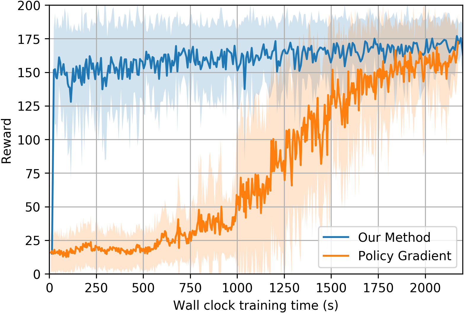
Figure 10: Wall-clock performance for pendulum

Although our method is adding a fraction of time for each epoch to conduct the projection step, the overall trend remains the same and the benefits from the ensured stability strictly out-weights the overhead.

References

- Abadi et al. (2015) Abadi, M.; Agarwal, A.; Barham, P.; Brevdo, E.; Chen, Z.; Citro, C.; Corrado, G. S.; Davis, A.; Dean, J.; Devin, M.; Ghemawat, S.; Goodfellow, I.; Harp, A.; Irving, G.; Isard, M.; Jia, Y.; Jozefowicz, R.; Kaiser, L.; Kudlur, M.; Levenberg, J.; Mané, D.; Monga, R.; Moore, S.; Murray, D.; Olah, C.; Schuster, M.; Shlens, J.; Steiner, B.; Sutskever, I.; Talwar, K.; Tucker, P.; Vanhoucke, V.; Vasudevan, V.; Viégas, F.; Vinyals, O.; Warden, P.; Wattenberg, M.; Wicke, M.; Yu, Y.; and Zheng, X. 2015. TensorFlow: Large-Scale Machine Learning on Heterogeneous Systems. Software available from tensorflow.org.
- Alleyne (1997) Alleyne, A. 1997. A comparison of alternative intervention strategies for unintended roadway departure (URD) control. Vehicle System Dynamics, 27(3): 157–186.
- Anderson et al. (2007) Anderson, C. W.; Young, P. M.; Buehner, M. R.; Knight, J. N.; Bush, K. A.; and Hittle, D. C. 2007. Robust reinforcement learning control using integral quadratic constraints for recurrent neural networks. IEEE Transactions on Neural Networks, 18(4): 993–1002.
- Athay, Podmore, and Virmani (1979) Athay, T.; Podmore, R.; and Virmani, S. 1979. A practical method for the direct analysis of transient stability. IEEE Transactions on Power Apparatus and Systems, (2): 573–584.
- Bai, Kolter, and Koltun (2019) Bai, S.; Kolter, J. Z.; and Koltun, V. 2019. Deep equilibrium models. In Advances in Neural Information Processing Systems, 688–699.
- Barto, Bradtke, and Singh (1995) Barto, A. G.; Bradtke, S. J.; and Singh, S. P. 1995. Learning to act using real-time dynamic programming. Artificial intelligence, 72(1-2): 81–138.
- Berkenkamp et al. (2017) Berkenkamp, F.; Turchetta, M.; Schoellig, A. P.; and Krause, A. 2017. Safe model-based reinforcement learning with stability guarantees. arXiv preprint arXiv:1705.08551.
- Boczar et al. (2017) Boczar, R.; Lessard, L.; Packard, A.; and Recht, B. 2017. Exponential stability analysis via integral quadratic constraints. arXiv preprint arXiv:1706.01337.
- Boyd et al. (1994) Boyd, S.; El Ghaoui, L.; Feron, E.; and Balakrishnan, V. 1994. Linear matrix inequalities in system and control theory. SIAM.
- Braziunas (2003) Braziunas, D. 2003. POMDP solution methods. University of Toronto.
- Callier and Desoer (2012) Callier, F. M.; and Desoer, C. A. 2012. Linear system theory. Springer Science & Business Media.
- Chakraborty, Seiler, and Balas (2011) Chakraborty, A.; Seiler, P.; and Balas, G. J. 2011. Susceptibility of F/A-18 flight controllers to the falling-leaf mode: Nonlinear analysis. Journal of guidance, control, and dynamics, 34(1): 73–85.
- Choi et al. (2020) Choi, J.; Castaneda, F.; Tomlin, C. J.; and Sreenath, K. 2020. Reinforcement learning for safety-critical control under model uncertainty, using control lyapunov functions and control barrier functions. arXiv preprint arXiv:2004.07584.
- Chow et al. (2018) Chow, Y.; Nachum, O.; Duenez-Guzman, E.; and Ghavamzadeh, M. 2018. A Lyapunov-based approach to safe reinforcement learning. arXiv preprint arXiv:1805.07708.
- Diamond and Boyd (2016) Diamond, S.; and Boyd, S. 2016. CVXPY: A Python-embedded modeling language for convex optimization. Journal of Machine Learning Research, 17(83): 1–5.
- Donti et al. (2020) Donti, P. L.; Roderick, M.; Fazlyab, M.; and Kolter, J. Z. 2020. Enforcing robust control guarantees within neural network policies. arXiv preprint arXiv:2011.08105.
- Doyle (1978) Doyle, J. C. 1978. Guaranteed margins for LQG regulators. IEEE Transactions on automatic Control, 23(4): 756–757.
- El Ghaoui et al. (2020) El Ghaoui, L.; Travacca, B.; Gu, F.; Tsai, A. Y.-T.; and Askari, A. 2020. Implicit Deep Learning. arXiv preprint arXiv:1908.06315.
- Fazel et al. (2018) Fazel, M.; Ge, R.; Kakade, S.; and Mesbahi, M. 2018. Global convergence of policy gradient methods for the linear quadratic regulator. In International Conference on Machine Learning, 1467–1476. PMLR.
- Fazelnia et al. (2016) Fazelnia, G.; Madani, R.; Kalbat, A.; and Lavaei, J. 2016. Convex relaxation for optimal distributed control problems. IEEE Transactions on Automatic Control, 62(1): 206–221.
- Fazlyab, Morari, and Pappas (2020) Fazlyab, M.; Morari, M.; and Pappas, G. J. 2020. Safety verification and robustness analysis of neural networks via quadratic constraints and semidefinite programming. IEEE Transactions on Automatic Control.
- Friedrich and Buss (2017) Friedrich, S. R.; and Buss, M. 2017. A robust stability approach to robot reinforcement learning based on a parameterization of stabilizing controllers. In 2017 IEEE International Conference on Robotics and Automation (ICRA), 3365–3372. IEEE.
- Gahinet and Apkarian (1994) Gahinet, P.; and Apkarian, P. 1994. A linear matrix inequality approach to control. International journal of robust and nonlinear control, 4(4): 421–448.
- Han et al. (2019) Han, M.; Tian, Y.; Zhang, L.; Wang, J.; and Pan, W. 2019. model-free reinforcement learning with robust stability guarantee. arXiv preprint arXiv:1911.02875.
- Heess et al. (2015) Heess, N.; Hunt, J. J.; Lillicrap, T. P.; and Silver, D. 2015. Memory-based control with recurrent neural networks. arXiv preprint arXiv:1512.04455.
- Jiang and Jiang (2012) Jiang, Y.; and Jiang, Z.-P. 2012. Computational adaptive optimal control for continuous-time linear systems with completely unknown dynamics. Automatica, 48(10): 2699–2704.
- Jin and Lavaei (2020) Jin, M.; and Lavaei, J. 2020. Stability-certified reinforcement learning: A control-theoretic perspective. IEEE Access.
- Kim, Patrón, and Braatz (2018) Kim, K. K.; Patrón, E. R.; and Braatz, R. D. 2018. Standard representation and unified stability analysis for dynamic artificial neural network models. Neural Networks, 98: 251–262.
- Kingma and Ba (2014) Kingma, D. P.; and Ba, J. 2014. Adam: A method for stochastic optimization. arXiv preprint arXiv:1412.6980.
- Knight and Anderson (2011) Knight, J. N.; and Anderson, C. 2011. Stable reinforcement learning with recurrent neural networks. Journal of Control Theory and Applications, 9(3): 410–420.
- Lessard, Recht, and Packard (2016) Lessard, L.; Recht, B.; and Packard, A. 2016. Analysis and design of optimization algorithms via integral quadratic constraints. SIAM Journal on Optimization, 26(1): 57–95.
- Levine (2021) Levine, S. 2021. CS285: Deep Reinforcement Learning. http://rail.eecs.berkeley.edu/deeprlcourse/. Course previously known as CS294: Deep Reinforcement Learning. Accessed: 2021-05-24.
- Levine et al. (2016) Levine, S.; Finn, C.; Darrell, T.; and Abbeel, P. 2016. End-to-end training of deep visuomotor policies. The Journal of Machine Learning Research, 17(1): 1334–1373.
- Levine and Koltun (2013) Levine, S.; and Koltun, V. 2013. Guided policy search. In International conference on machine learning, 1–9. PMLR.
- Levine et al. (2018) Levine, S.; Pastor, P.; Krizhevsky, A.; Ibarz, J.; and Quillen, D. 2018. Learning hand-eye coordination for robotic grasping with deep learning and large-scale data collection. The International Journal of Robotics Research, 37(4-5): 421–436.
- Lillicrap et al. (2016) Lillicrap, T. P.; Hunt, J. J.; Pritzel, A.; Heess, N.; Erez, T.; Tassa, Y.; Silver, D.; and Wierstra, D. 2016. Continuous control with deep reinforcement learning. In ICLR (Poster).
- Luo, Wu, and Huang (2014) Luo, B.; Wu, H.-N.; and Huang, T. 2014. Off-policy reinforcement learning for control design. IEEE transactions on cybernetics, 45(1): 65–76.
- Matni et al. (2019) Matni, N.; Proutiere, A.; Rantzer, A.; and Tu, S. 2019. From self-tuning regulators to reinforcement learning and back again. In 2019 IEEE 58th Conference on Decision and Control (CDC), 3724–3740. IEEE.
- Megretski and Rantzer (1997) Megretski, A.; and Rantzer, A. 1997. System analysis via integral quadratic constraints. IEEE Transactions on Automatic Control, 42(6): 819–830.
- Mnih et al. (2015) Mnih, V.; Kavukcuoglu, K.; Silver, D.; Rusu, A. A.; Veness, J.; Bellemare, M. G.; Graves, A.; Riedmiller, M.; Fidjeland, A. K.; Ostrovski, G.; et al. 2015. Human-level control through deep reinforcement learning. nature, 518(7540): 529–533.
- Monahan (1982) Monahan, G. E. 1982. State of the art—a survey of partially observable Markov decision processes: theory, models, and algorithms. Management science, 28(1): 1–16.
- Morimoto and Doya (2005) Morimoto, J.; and Doya, K. 2005. Robust reinforcement learning. Neural computation, 17(2): 335–359.
- Mundhenk et al. (2000) Mundhenk, M.; Goldsmith, J.; Lusena, C.; and Allender, E. 2000. Complexity of finite-horizon Markov decision process problems. Journal of the ACM (JACM), 47(4): 681–720.
- Pauli et al. (2021) Pauli, P.; Gramlich, D.; Berberich, J.; and Allgöwer, F. 2021. Linear systems with neural network nonlinearities: Improved stability analysis via acausal Zames-Falb multipliers. arXiv preprint arXiv:2103.17106.
- Recht (2019) Recht, B. 2019. A tour of reinforcement learning: The view from continuous control. Annual Review of Control, Robotics, and Autonomous Systems, 2: 253–279.
- Revay, Wang, and Manchester (2020) Revay, M.; Wang, R.; and Manchester, I. R. 2020. A Convex Parameterization of Robust Recurrent Neural Networks. IEEE Control Systems Letters, 5(4): 1363–1368.
- Sastry (2013) Sastry, S. 2013. Nonlinear systems: analysis, stability, and control, volume 10. Springer Science & Business Media.
- Scherer, Gahinet, and Chilali (1997) Scherer, C.; Gahinet, P.; and Chilali, M. 1997. Multiobjective output-feedback control via LMI optimization. IEEE Transactions on automatic control, 42(7): 896–911.
- Schwenkel et al. (2021) Schwenkel, L.; Köhler, J.; Müller, M. A.; and Allgöwer, F. 2021. Model predictive control for linear uncertain systems using integral quadratic constraints. arXiv preprint arXiv:2104.05444.
- Silver et al. (2016) Silver, D.; Huang, A.; Maddison, C. J.; Guez, A.; Sifre, L.; Van Den Driessche, G.; Schrittwieser, J.; Antonoglou, I.; Panneershelvam, V.; Lanctot, M.; et al. 2016. Mastering the game of Go with deep neural networks and tree search. nature, 529(7587): 484–489.
- Sutton and Barto (2018) Sutton, R. S.; and Barto, A. G. 2018. Reinforcement learning: An introduction. MIT press.
- Sutton et al. (1999) Sutton, R. S.; McAllester, D. A.; Singh, S. P.; Mansour, Y.; et al. 1999. Policy gradient methods for reinforcement learning with function approximation. In NIPs, volume 99, 1057–1063. Citeseer.
- Talpaert et al. (2019) Talpaert, V.; Sobh, I.; Kiran, B. R.; Mannion, P.; Yogamani, S.; El-Sallab, A.; and Perez, P. 2019. Exploring applications of deep reinforcement learning for real-world autonomous driving systems. arXiv preprint arXiv:1901.01536.
- Tobenkin, Manchester, and Megretski (2017) Tobenkin, M. M.; Manchester, I. R.; and Megretski, A. 2017. Convex parameterizations and fidelity bounds for nonlinear identification and reduced-order modelling. IEEE Transactions on Automatic Control, 62(7): 3679–3686.
- Van Rossum and Drake (2009) Van Rossum, G.; and Drake, F. L. 2009. Python 3 Reference Manual. Scotts Valley, CA: CreateSpace. ISBN 1441412697.
- Wierstra et al. (2007) Wierstra, D.; Foerster, A.; Peters, J.; and Schmidhuber, J. 2007. Solving deep memory POMDPs with recurrent policy gradients. In International conference on artificial neural networks, 697–706. Springer.
- Williams (1992) Williams, R. J. 1992. Simple statistical gradient-following algorithms for connectionist reinforcement learning. Machine learning, 8(3-4): 229–256.
- Wright and Ma (2021) Wright, J.; and Ma, Y. 2021. High-Dimensional Data Analysis with Low-Dimensional Models: Principles, Computation, and Applications. Cambridge University Press.
- Yakubovich (1971) Yakubovich, V. 1971. S-procedure in nonlinear control theory (in Russian). In Vestnik Leningrad. Univ.
- Yin, Seiler, and Arcak (2021) Yin, H.; Seiler, P.; and Arcak, M. 2021. Stability analysis using quadratic constraints for systems with neural network controllers. IEEE Transactions on Automatic Control.
- Yin et al. (2021) Yin, H.; Seiler, P.; Jin, M.; and Arcak, M. 2021. Imitation learning with stability and safety guarantees. IEEE Control Systems Letters.
- Zhang, Hu, and Basar (2020) Zhang, K.; Hu, B.; and Basar, T. 2020. Policy Optimization for Linear Control with Robustness Guarantee: Implicit Regularization and Global Convergence. In Learning for Dynamics and Control, 179–190. PMLR.
- Zhang et al. (2016) Zhang, M.; McCarthy, Z.; Finn, C.; Levine, S.; and Abbeel, P. 2016. Learning deep neural network policies with continuous memory states. In 2016 IEEE international conference on robotics and automation (ICRA), 520–527. IEEE.
- Zheng, Tang, and Li (2021) Zheng, Y.; Tang, Y.; and Li, N. 2021. Analysis of the Optimization Landscape of Linear Quadratic Gaussian (LQG) Control. arXiv preprint arXiv:2102.04393.
- Zhou et al. (1996) Zhou, K.; Doyle, J. C.; Glover, K.; et al. 1996. Robust and optimal control, volume 40. Prentice hall New Jersey.