The MOSDEF Survey: The Dependence of H$\alpha$-to-UV SFR Ratios on SFR and Size at $z\sim 2$

Abstract

We perform an aperture-matched analysis of dust-corrected H$\alpha$ and UV SFRs using 303 star-forming galaxies with spectroscopic redshifts $1.36<z_{\text{spec}}<2.66$ from the MOSFIRE Deep Evolution Field (MOSDEF) survey. By combining H$\alpha$ and H$\beta$ emission line measurements with multi-waveband resolved CANDELS/3D-HST imaging, we directly compare dust-corrected H$\alpha$ and UV SFRs, inferred assuming a fixed attenuation curve shape and constant SFHs, within the spectroscopic aperture. Previous studies have found that H$\alpha$ and UV SFRs inferred with these assumptions generally agree for typical star-forming galaxies, but become increasingly discrepant for galaxies with higher SFRs ($\gtrsim$100 $M_{\odot}$ yr^-1), with H$\alpha$-to-UV SFR ratios being larger for these galaxies. Our analysis shows that this trend persists even after carefully accounting for the apertures over which H$\alpha$ and UV-based SFRs (and the nebular and stellar continuum reddening) are derived. Furthermore, our results imply that H$\alpha$ SFRs may be higher in the centers of large galaxies (i.e., where there is coverage by the spectroscopic aperture) compared to their outskirts, which could be indicative of inside-out galaxy growth. Overall, we suggest that the persistent difference between nebular and stellar continuum reddening and high H$\alpha$-to-UV SFR ratios at the centers of large galaxies may be indicative of a patchier distribution of dust in galaxies with high SFRs.

1 Introduction

Galaxies were rapidly assembling their stellar mass at $z\sim 2$ when cosmic star-formation activity was at its peak (see Madau & Dickinson, 2014). An important measure of how galaxies build their stellar mass is their star-formation rate (SFR). The SFR of galaxies in the local universe has been probed by observations of the ultraviolet (UV) continuum, nebular emission lines (e.g., H$\alpha$, H$\beta$, Br$\gamma$), mid- and far-infrared (IR) continuum, radio continuum, X-ray emission, and combinations of these tracers (e.g., Kennicutt, 1998; Kennicutt & Evans, 2012; Hao et al., 2011). SFR measurements for higher redshift galaxies, however, typically rely on a limited set of tracers. For example, at higher redshifts, the longer-wavelength tracers are of limited use as typical unlensed galaxies are not directly detected at these wavelengths. As such, we must rely on SFR indicators that can be accessed for individual high-redshift galaxies (e.g., UV continuum, H$\alpha$, H$\beta$), but which may require corrections for the obscuring effects of dust.

Dust obscuration can be directly probed by comparing the measured Balmer decrement (H$\alpha$/H$\beta$) to the intrinsic Balmer decrement expected from typical conditions in the interstellar medium (ISM; Osterbrock, 1989). This method is sensitive to the reddening towards the youngest stellar populations that host the most massive stars. An alternative method for estimating dust obscuration is to measure the slope of the UV continuum (Calzetti et al., 1994; Meurer et al., 1999), which is sensitive to stars over a broader range of stellar mass compared to the Balmer decrement. In general, these two measures for obscuration cannot be used interchangeably. Several studies of high-redshift galaxies have noted higher reddening towards the most massive stars ($E(B-V)_{\text{gas}}$) compared to the stellar continuum ($E(B-V)_{\text{stars}}$) by a constant factor (e.g., Meurer et al., 1999; Calzetti et al., 2000; Kashino et al., 2013; Price et al., 2014; Tacchella et al., 2018) or as a function of SFR (Yoshikawa et al., 2010; Kreckel et al., 2013; Reddy et al., 2015), specific SFR (Wild et al., 2011; Price et al., 2014; Boquien et al., 2015; Reddy et al., 2015; Hemmati et al., 2015), SFR surface density (Boquien et al., 2015), and gas-phase metallicity (Shivaei et al., 2020).

Once appropriate dust corrections have been applied, H$\alpha$ and UV SFRs have been found to generally agree for most typical star-forming galaxies at high redshifts (e.g., Erb et al., 2006; Reddy et al., 2010; Wuyts et al., 2013; Steidel et al., 2014; Reddy et al., 2015; Shivaei et al., 2015a, 2020; Theios et al., 2019; Shivaei et al., 2020). However, some authors have found that SFRs derived from nebular emission lines are systematically higher than those inferred from the UV continuum in high-redshift galaxies with high SFRs ($\gtrsim$100 $M_{\odot}$ yr^-1; Hao et al., 2011; Reddy et al., 2015; Katsianis et al., 2017). Variations in SFRs derived using different tracers may result from their sensitivity to star formation on different timescales (Reddy et al., 2012b; Price et al., 2014), which could provide useful information about the initial mass function (IMF) or star-formation history (SFH) of galaxies (Madau & Dickinson, 2014), or could alternatively be caused by incorrect assumptions regarding dust corrections.

A non-uniform distribution of dust and stars has been invoked to explain the observed differences between nebular and stellar continuum reddening (Calzetti et al., 1994; Wild et al., 2011; Price et al., 2014; Reddy et al., 2020), and could also potentially explain the observed differences between SFRs inferred from H$\alpha$ and UV data (Boquien et al., 2009, 2015; Hao et al., 2011; Reddy et al., 2015; Katsianis et al., 2017). The young massive stars that dominate the nebular line emission ($\gtrsim$15 $M_{\odot}$; Kennicutt & Evans, 2012) may be enshrouded in their parent birth clouds, while the UV continuum is dominated by stars over a larger range of main sequence lifetimes (10–200 Myr; Kennicutt & Evans, 2012). However, some of the less massive O and B stars will survive the dissipation of their birth clouds (Calzetti et al., 1994; Boquien et al., 2015; Faisst et al., 2017; Narayanan et al., 2018) and will disproportionally add to the UV continuum light compared to more obscured OB associations. Furthermore, the nebular emission coming from the OB associations that have escaped their heavily obscured birth clouds will be overall less dust reddened—with reddening that is more similar to that which is typical of the UV continuum—compared to younger OB associations. Therefore, the dust that is reddening the nebular emission could also originate from the ionized or neutral gas phase of the ISM, such that the differences between the nebular and stellar continuum reddening may not necessarily be exclusively connected to the dust proximate to the youngest OB associations (Reddy et al., 2020).

In addition to causing inconsistent SFR and reddening estimates, if geometrical effects within galaxies are at play, then the assumptions that are used to correct spectroscopic emission line measurements for light falling outside of the slit aperture may not be robust (Brinchmann et al., 2004; Kewley et al., 2005; Salim et al., 2007; Richards et al., 2016; Green et al., 2017). Putting aside the dust corrections, if the spectroscopic emission line measurements are not corrected for slit-loss, then H$\alpha$ SFRs, which are typically determined from spectroscopic observations, would lie systematically lower than UV SFRs, which are typically inferred from broadband photometry. Additionally, total H$\alpha$ SFRs could also be over or underestimated if inappropriate assumptions are made about the Balmer decrement or if one assumes a flat H$\alpha$ light profile, in contrast to the centrally-peaked H$\alpha$ profiles observed in $z\sim 2$ galaxies where H$\alpha$ surface brightness decreases with increasing galactocentric distance (e.g., Nelson et al., 2013, 2016; Hemmati et al., 2015; Tacchella et al., 2018). Furthermore, the average Balmer decrement measured across the spectroscopic slit may not necessarily be indicative of the globally-averaged Balmer decrement and could contribute to any discrepancies between $E(B-V)_{\text{gas}}$ and the globally-measured $E(B-V)_{\text{stars}}$. Therefore, it is important to identify the significance of any “aperture” biases when comparing spectroscopic measurements of nebular emission lines with measurements of the UV continuum, the latter of which is typically performed on the whole galaxy.

In this study, we investigate how aperture effects influence the interpretation of reddening and SFRs derived from the UV continuum and nebular emission line observations. We pair rest-frame optical spectra from the MOSFIRE Deep Evolution Field survey (MOSDEF; Kriek et al., 2015) with multi-waveband resolved imaging from the Cosmic Assembly Near-infrared Deep Extragalactic Legacy Survey (CANDELS; Grogin et al., 2011; Koekemoer et al., 2011) and the broadband photometric catalog compiled by the 3D-HST survey (Brammer et al., 2012; Skelton et al., 2014). The MOSDEF survey obtained rest-frame optical spectra for $\sim$1500 star-forming and AGN galaxies at $1.4\lesssim z\lesssim 3.8$. Here we take advantage of the statistically large MOSDEF spectroscopic survey by analyzing a sample of 303 star-forming galaxies with detected H$\alpha$ and H$\beta$ emission at $z\sim 2$.

The data and sample selection are presented in Section 2. In Section 3, we describe our methodology for measuring dust-corrected H$\alpha$ and UV SFRs directly within the MOSFIRE spectroscopic slit region. We then compare the globally measured dust-corrected SFRs to those measured inside the spectroscopic aperture in Section 4 and discuss our findings in Section 5. Finally, our results are summarized in Section 6.

Throughout this paper, we assume a cosmology with $H_{0}=70$ km s^-1 Mpc^-1, ${\Omega_{\Lambda}=0.7}$, and ${\Omega_{m}=0.3}$. All line wavelengths are in vacuum and all magnitudes are expressed in the AB system (Oke & Gunn, 1983). For clarity, we refer to all reddening and SFR measurements made over the entire galaxy area as “global” measurements.

2 Data and Sample Selection

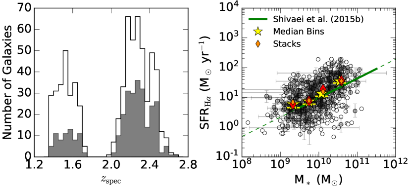
Figure 1: Left: The distribution of spectroscopic redshifts for the sample covering two redshift bins: $1.24<z<1.74$ and $1.99<z<2.66$. The spectroscopic redshifts of the initial sample (675 galaxies) are shown by the white histogram. The final sample (303 galaxies), where all galaxies are detected with a $S/N\geq 3$ in H$\alpha$ and H$\beta$ emission, is denoted by the gray histogram. Right: The sample relative to the star-forming H$\alpha$ SFR–$M_{*}$ relation. H$\alpha$ emission is corrected for dust reddening by using the Balmer decrement and assuming the Cardelli et al. (1989) extinction curve. A Chabrier (2003) IMF and 20% solar metallicity is also also assumed when calculating H$\alpha$ SFRs (see Section 3.3). The linear relation that is best-fit to the star-forming SFR–$M_{*}$ relation using the first two years of data from the MOSDEF survey (Shivaei et al., 2015b) is shown by the solid green line and is extended with a dashed line for visual clarity. The MOSDEF spectra are stacked in four equal bins of stellar mass for both the initial (large red diamonds) and final (small orange diamonds) samples, respectively, showing that the sample is not biased against the dustiest galaxies where H$\beta$ is not detected. The galaxies in the initial (675) and final (303) samples are shown by the empty and filled circles, respectively. The sample is also divided equally into four bins of stellar mass to show the medians of the individual measurements for the 303 galaxies in the sample (yellow stars).

2.1 CANDELS/3D-HST Photometry

CANDELS observed $\sim$900 arcmin² of the sky and achieved 90% completeness at $H_{160}\sim 25$ mag covering five well-studied extragalactic fields: AEGIS, COSMOS, GOODS-N, GOODS-S, and UDS (Grogin et al., 2011; Koekemoer et al., 2011). We use the multi-wavelength HST/WFC3 (F125W, F140W, and F160W filters, hereafter $J_{125}$, $JH_{140}$, and $H_{160}$) and HST/ACS (F435W, F606W, F775W, F814W, and F850LP filters, hereafter $B_{435}$, $V_{606}$, $i_{775}$, $I_{814}$, and $z_{850}$) resolved CANDELS imaging that has been processed by the 3D-HST grism survey team (Brammer et al., 2012; Skelton et al., 2014; Momcheva et al., 2016). The publicly-available processed CANDELS images have been drizzled to a 0$\aas@@fstack{\prime\prime}$06 pix^-1 scale and PSF-convolved to the spatial resolution of the $H_{160}$ imaging (0$\aas@@fstack{\prime\prime}$18). We also use the broadband photometric catalogs provided by the 3D-HST team, which cover 0.3 to 8.0 $\mu$m in the five extragalactic CANDELS fields.

2.2 MOSDEF Spectroscopy

Targets were selected for the MOSDEF survey in three redshift bins ($1.37<z<1.70$, $2.09<z<2.61$, and $2.95<z<3.80$) using the 3D-HST photometric and spectroscopic catalogs. In order to reach a stellar mass limit of $\sim$10⁹ $M_{\odot}$ for all three redshift bins, an $H_{160}$-band limit of 24.0, 24.5, and 25.0 mag was used for the $z\sim 1.5$, $z\sim 2.3$, and $z\sim 3$ bins, respectively. These redshift bins were selected such that the following strong rest-frame optical emission lines fall in near-IR windows of atmospheric transmission: [OII]$\lambda 3727,3730$, H$\beta$, [OIII]$\lambda\lambda 4960,5008$, H$\alpha$, [NII]$\lambda\lambda 6550,6585$, and [SII]$\lambda 6718,6733$.

Observations for the MOSDEF survey were taken over 48.5 nights in 2012–2016 on the 10 m Keck I telescope using the MOSFIRE multi-object spectrograph (McLean et al., 2010, 2012) in the $Y$, $J$, $H$, and $K$ bands ($R=3400$, 3000, 3650, and 3600 using 0$\aas@@fstack{\prime\prime}$7 slit widths). Rest-frame optical spectra were obtained for $\sim$1500 galaxies at $1.4\lesssim z\lesssim 3.8$. Every slit mask included at least one slit star, which is used, in part, for the absolute flux calibration of the spectra and to correct for slit losses. The procedures for correcting for slit loss and measuring line fluxes are described in Section 2.2.1 and Section 2.2.2, respectively. See Kriek et al. (2015) for further details on the MOSDEF survey, including the observation strategy and data reduction.

2.2.1 Slit-loss Corrections

The slit loss estimated from the slit star is dependent on seeing conditions. Therefore, emission lines that are measured from different bandpasses (such as H$\alpha$ and H$\beta$) for a given galaxy will have different slit-loss corrections. Given that the typical seeing during the observations is comparable to the slit width of 0$\aas@@fstack{\prime\prime}$7, using a point source slit star is insufficient to correct the spatially-resolved MOSDEF galaxy targets for light lost outside of the spectroscopic slit. Therefore, to best account for additional slit loss, a secondary correction is applied to the spectrum of each galaxy in each near-IR filter. This correction is based on a 2D rotated elliptical Gaussian that is fit to the 3D-HST $H_{160}$ image of the galaxy that has been convolved to the typical seeing during the observation through the relevant filter (Reddy et al., 2015).

2.2.2 Line Flux Measurements

Line fluxes are measured by fitting a linear function to the continuum and a Gaussian function to each emission line, with double and triple Gaussians fit to the [OII]$\lambda\lambda 3727,3730$ doublet and H$\alpha$+[NII]$\lambda\lambda 6550,6585$ lines, respectively. H$\alpha$ and H$\beta$ line fluxes are corrected for underlying Balmer absorption using the stellar population model that best fits the observed 3D-HST broadband photometry (Section 3.2). Flux errors are obtained by perturbing the 1D spectra by their error spectra 1000 times, remeasuring the line fluxes, and taking the 68th-percentile width of the distribution. Finally, the observed wavelength of the highest signal-to-noise ($S/N$) line, which is usually H$\alpha$ or [OIII]$\lambda 5008$, is used to measure the spectroscopic redshift. For more details on the emission line flux measurements, see Reddy et al. (2015).

2.3 Sample Selection

The sample is derived from the MOSDEF parent sample in the $z\sim 1.5$ and $z\sim 2.3$ redshift bins, where both the H$\alpha$ and H$\beta$ emission lines are covered by the ground-based spectroscopy. In order to optimally measure Balmer decrements and correct for slit loss, both H$\alpha$ and H$\beta$ are required to be detected with a $S/N\geq 3$. However, we also consider an “initial” sample where H$\beta$ is undetected ($S/N<3$), but still covered by the observations, to investigate a possible bias against the dustiest galaxies. AGNs are identified through their X-ray luminosities, optical emission lines ($\log{(\text{[NII]/H}\alpha)}>-0.3$), and/or mid-IR luminosities (Coil et al., 2015; Azadi et al., 2017, 2018; Leung et al., 2019), then removed from the sample.

With these requirements, the initial and primary samples include 675 and 449 star-forming galaxies, respectively, at $1.24<z<2.66$. The primary sample includes 19 galaxies that fall outside of the targeted MOSDEF redshift bins, as these targets were serendipitously detected. When the CANDELS HST images are smoothed to the seeing of the MOSFIRE observations (see Section 3.1), 25 galaxies are undetected in the segmentation maps based on the smoothed images and are removed from the sample. After modeling the stellar populations globally and within the slit area (see Section 3.2), we find that the SED-derived SFRs (i.e., UV SFRs) of 112 galaxies are measured to be higher inside the slit than across the entire galaxy—which is unphysical and primarily caused by key features of the SED being unconstrained (e.g., UV slope, Balmer/4000 Å breaks; see Section 3.2). Therefore, these galaxies are removed from the sample along with an additional 9 galaxies that have poorly constrained photometry, resulting in a final sample size of 303 star-forming galaxies at $1.36<z<2.66$.

Figure 1 shows the spectroscopic redshift distribution and SFR–$M_{*}$ relation for the galaxies in the primary sample (303 galaxies; filled gray circles) compared to the initial sample (675 galaxies; empty circles). As a visual aid, the sample is divided into four equally sized bins and their medians in SFR and stellar mass are shown (yellow stars). The values for the median bins are on average 0.14 dex above the Shivaei et al. (2015b) SFR–$M_{*}$ relation, which was defined by the star-forming galaxies observed during the first two years of the MOSDEF survey. To ensure that we are not biasing the sample against the dustiest galaxies by removing all of those where H$\beta$ is undetected, stacks of the spectra are constructed using specline (Shivaei et al., 2018) in four bins of stellar mass for the galaxies in the initial (675 galaxies; large red diamonds) and the final (303 galaxies; small orange diamonds) samples. If our sample was biased against the dustiest galaxies, the stacks of the final sample (small orange diamonds) would be systematically higher than the stacks of the initial sample (large red diamonds) since $E(B-V)_{\text{gas}}$ is used to correct SFR${}_{\text{H}\alpha}$ (see dust-corrected SFR${}_{\text{H}\alpha}$ in Section 3.3). The right panel of Figure 1 shows that the two sets of stacked bins are comparable within their uncertainties, are within the intrinsic scatter of the Shivaei et al. (2015b) SFR–$M_{*}$ relation, and the final sample (small orange diamonds) is not systematically biased towards higher SFR${}_{\text{H}\alpha}$. Furthermore, stacking all of the H$\beta$ non-detections (226 galaxies) into a single bin reveals a Balmer Decrement measurement (H$\alpha$/H$\beta$ $=4.13\pm 0.74$) that is within $1\sigma$ of the average Balmer Decrement for the galaxies in our final sample (H$\alpha$/H$\beta$ $=3.47\pm 0.19$). Visual inspection of the spectra reveals that H$\beta$ non-detections for MOSDEF targets are often due to contamination from skylines rather than H$\beta$ falling below the detection threshold (Reddy et al., 2015; Shivaei et al., 2015b; Sanders et al., 2018). Thus, the sample is not significantly biased against the dustiest galaxies when H$\beta$ non-detections are excluded from the sample.

3 Methodology and Measurements

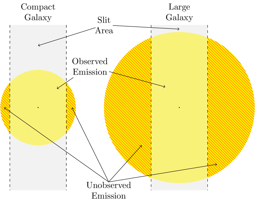
Figure 2: Visualization of how the spectroscopic slit covers compact versus large galaxies. The gray region between the dashed vertical lines represents the spectroscopic slit area, which is centered (black dot) on the light distribution of each galaxy (yellow circles) measured from the photometry. Only the emission within the slit area is directly observed in the spectroscopy, whereas any emission that lies outside of the slit area (red hatched regions) is not directly observed.

In this section, we outline our procedure for calculating dust-corrected SFRs measured from H$\alpha$ emission and the UV stellar continuum. H$\alpha$ and H$\beta$ emission measured from slit spectroscopy (and other observed spectroscopic measurements) do not include information about the regions of the galaxy lying outside of the slit area, as is illustrated in Figure 2. The slit-loss corrections applied to the MOSDEF spectroscopic observations assume a certain light profile for the galaxy based on a single filter (see Section 2.2.1). This simple light profile may not be sufficiently accurate for large galaxies where a significant fraction of their light falls outside the slit area or which may have light profiles that vary significantly from band-to-band. Furthermore, the position of the slit is randomly oriented relative to the physical structure of individual galaxies in order to optimize their placement on the MOSFIRE mask for multi-object spectroscopy. The UV light, however, is typically measured over an area larger than the spectroscopic slit, usually a circular or isophotal aperture in the imaging. Thus, to make a truly fair comparison between H$\alpha$ and UV SFRs, we must measure them over the same spatial area, or aperture.

First, we describe the image smoothing and flux measurements accounting for resolution and area in Section 3.1. In Section 3.2, we present the SED fitting procedure that is used to obtain both the global and slit-measured stellar population properties, from which $E(B-V)_{\text{stars}}$ is directly inferred. Finally, in Section 3.3, we detail our methods for obtaining $E(B-V)_{\text{gas}}$, H$\alpha$ SFRs, and UV SFRs.

3.1 Image Smoothing

The seeing of the MOSFIRE observations was typically $\sim$0$\aas@@fstack{\prime\prime}$7. For comparison, the FWHM of the HST $H_{160}$ PSF is $\sim$0$\aas@@fstack{\prime\prime}$18. Therefore, in order to directly compare measurements made from the resolved imaging with the spectroscopic measurements, the HST images are first smoothed to match the typical seeing of the MOSFIRE observations. The astropy.convolution python package (Astropy Collaboration et al., 2013, 2018) is used to convolve the HST images with a 2D gaussian kernel with FWHM $\sigma_{\text{kernel}}=\sqrt{\sigma_{\text{MOSFIRE}}^{2}-\sigma_{\text{HST}}^{2}}$, where $\sigma_{\text{HST}}$ is the FWHM of the HST PSF equal to 0$\aas@@fstack{\prime\prime}$18, and $\sigma_{\text{MOSFIRE}}$ is the FWHM of the seeing from the MOSFIRE observations. This smoothing procedure is repeated assuming $\sigma_{\text{MOSFIRE}}$ is 0$\aas@@fstack{\prime\prime}$5–0$\aas@@fstack{\prime\prime}$9 in 0$\aas@@fstack{\prime\prime}$1 increments, to account for variations in the seeing during the MOSFIRE observations. The smoothed images that are selected for an individual galaxy depends on the average seeing during the respective MOSFIRE observations ($\sigma_{\text{MOSFIRE}}$). RMS maps corresponding to the smoothed HST images are constructed by scaling the original RMS maps such that the S/N is preserved in each pixel (see Fetherolf et al., 2020).

A segmentation map based on the smoothed images is generated by using a noise-equalized $J_{125}$+$JH_{140}$+$H_{160}$ smoothed image for source detection and following the same input parameters for Source Extractor (Bertin & Arnouts, 1996) as Skelton et al. (2014). There are 25 galaxies from the sample that are undetected in the segmentation map of the smoothed images and, thus, are removed from the sample. The smoothed images that assume a $\sigma_{\text{MOSFIRE}}$ that best matches the MOSFIRE seeing from the observations of each galaxy are used to measure fluxes and perform SED fitting (see Section 3.2).

Pixels that fall inside the slit area are identified using the source centroid, mask position angle, and slit width. The counts from the smoothed images for the pixels inside the slit are summed and converted to AB magnitude and the magnitude error is determined similarly (except summed in quadrature) from the noise maps. In order to avoid any single photometric point from skewing the SED fit, the minimum magnitude error is restricted to be no smaller than 0.05 mag.

To better constrain the shape of the SED at longer wavelengths, the resolved CANDELS imaging are supplemented with unresolved Spitzer/IRAC photometry at 3.6 $\mu$m, 4.5 $\mu$m, 5.8 $\mu$m, and 8.0 $\mu$m available from the 3D-HST broadband photometry catalog (Skelton et al., 2014). The Spitzer/IRAC photometry has been corrected for contamination by neighboring sources using models of the HST images that have been PSF-smoothed to the lower resolution IRAC photometry. Source pixels were identified from the segmentation maps. In order to include the IRAC photometry with the photometric slit measurements for SED fitting, the total IRAC fluxes from the 3D-HST broadband photometric catalog, $F_{\text{IRAC,tot}}$, are normalized using the $H_{160}$ flux measured inside the slit area from the smoothed imaging, $H_{160,\text{slit}}$, as follows:

$$F_{\text{IRAC,slit}}=F_{\text{IRAC,tot}}\frac{H_{160,\text{slit}}}{H_{160,\text{tot}}}\text{,}$$ (1)

where $H_{160,\text{tot}}$ is the total $H_{160}$ flux measured from the 3D-HST broadband photometry and $F_{\text{IRAC,slit}}$ is the resultant normalized IRAC flux. On scales smaller than the slit width Fetherolf et al. (2020) showed that incorporating the IRAC photometry into the SED fitting using Equation 1 does not significantly affect the derived stellar population properties.

3.2 SED Fitting

The total and slit-measured fluxes are modeled, as follows, to obtain SED-derived $E(B-V)_{\text{stars}}$, stellar population ages, SFRs, and stellar masses. First, the contribution of the strongest emission lines measured in the MOSFIRE spectra (i.e., [OII]$\lambda\lambda 3727,3730$, H$\beta$, [OIII]$\lambda\lambda 4960,5008$, and H$\alpha$) is removed from the broadband photometry. We use $\chi^{2}$ minimization to select the Bruzual & Charlot (2003) stellar population synthesis model that best fits the photometry assuming a Chabrier (2003) IMF, SMC extinction curve (Fitzpatrick & Massa, 1990; Gordon et al., 2003), and sub-solar metallicity (0.2 $Z_{\odot}$). Reddening is allowed to vary in the range $0.0\leq\mbox{$E(B-V)_{\text{stars}}$}\ \leq 0.4$. Only constant SFHs and stellar ages between 50 Myr and the age of the Universe at the redshift of each galaxy are considered. Finally, the measured photometric fluxes are perturbed 100 times by the flux errors and the $1\sigma$ SED parameter uncertainties are determined by the range of parameters inferred for the 68 models with the lowest $\chi^{2}$.

There are 112 galaxies that exhibit SED-derived SFRs that are unphysically larger when measured inside the slit area than across the entire galaxy. We consider the SFRs measured inside the slit to be inaccurate in these cases considering that they are based on significantly fewer and less precise photometric measurements. Fetherolf et al. (2020) showed that if the photometry does not constrain key features of the SED (e.g., UV slope, Balmer/4000 Å break) either by wavelength coverage or sufficient S/N, then the SED-derived parameters may be biased towards redder $E(B-V)_{\text{stars}}$ and younger stellar population ages while stellar masses remain robust. Overestimated reddening and underestimated stellar ages (at constant stellar mass and SFH) can, in turn, lead to underestimated SFRs. All 112 galaxies that exhibit overestimated SED-derived SFRs inside the slit exhibit $E(B-V)_{\text{stars}}$ and stellar ages that are both redder and younger than the globally averaged $E(B-V)_{\text{stars}}$ and stellar ages. On the other hand, the average differences between global and slit-measured $E(B-V)_{\text{stars}}$ and $\log(\text{Age/yr})$ for the other 312 galaxies are only 0.03 mag and 0.09 dex, respectively. Furthermore, 98 of the 112 galaxies with overestimated slit-measured SED SFRs have less than two photometric points with a $S/N\geq 1$ covering the UV slope (1250–2500 Å), and thus this region of the SED is not well-constrained for these galaxies. There are also an additional 9 galaxies that do not have well-constrained photometric measurements from the resolved imaging. For these reasons, we remove from the sample a total of 121 galaxies that do not have robust constraints on the UV slope.

3.3 $E(B-V)_{\text{gas}}$ and SFR Calculations

 

 

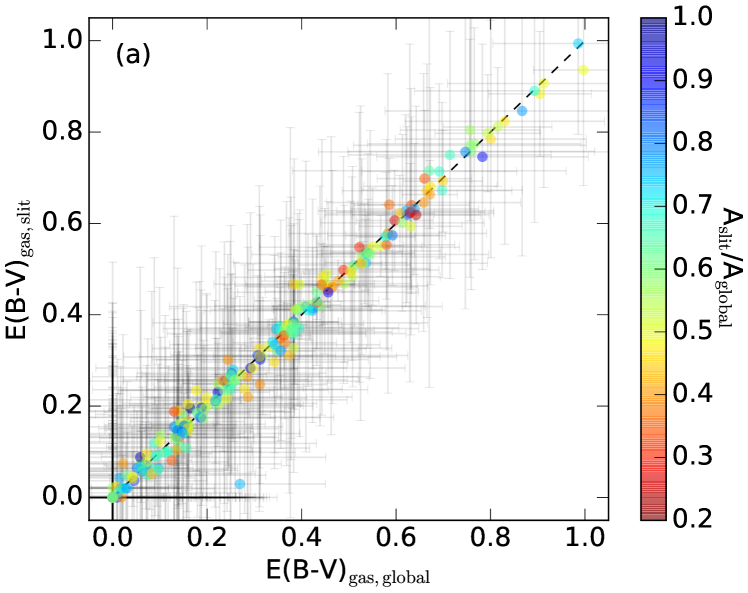
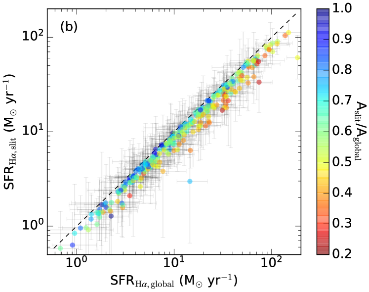
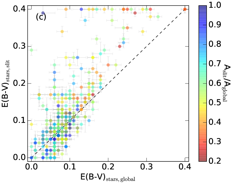
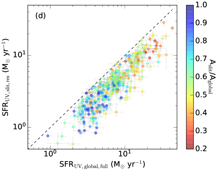
Figure 3: Left: Nebular (panel a) and stellar continuum (panel c) reddening obtained from the spectroscopic slit area compared to the inferred global reddening. Right: SFR${}_{\text{H}\alpha}$ (panel b) and SFR${}_{\text{UV}}$ (panel d) derived from the slit area versus the global SFRs. The points are colored by the fraction of the galaxy that falls within the slit area (see Figure 2). The black dashed lines show where the global and slit-derived reddening and SFRs are equal.

 

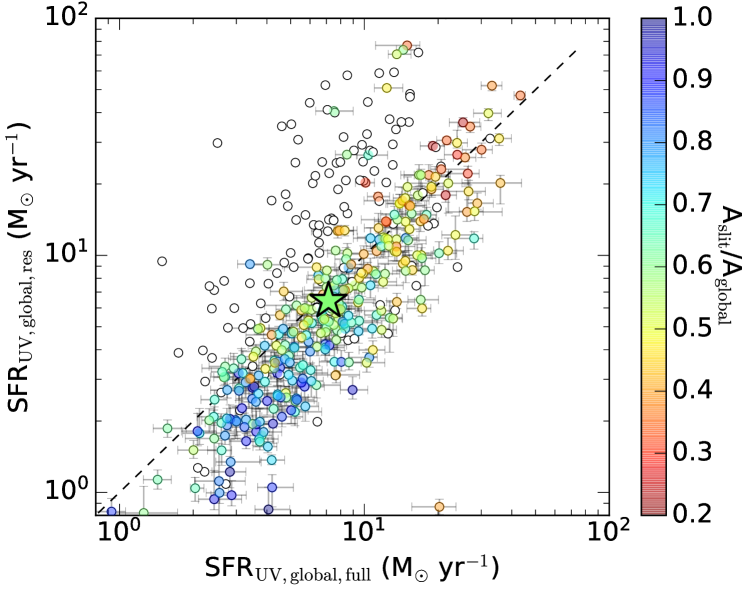
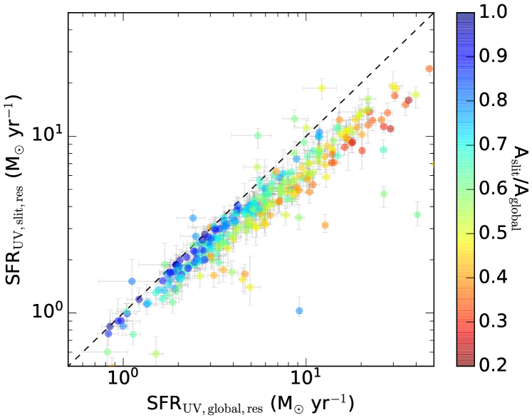
Figure 4: Left: SFR${}_{\text{UV,global}}$ derived from an SED fit to 3D-HST photometric catalog, which has extended wavelength coverage, compared to those derived from the summed flux of only the resolved CANDELS/3D-HST imaging. The dashed line shows where the two SFR${}_{\text{UV}}$ measurements are equal. The points are colored by the fraction of the galaxy that falls within the slit area (see Figure 2). The white empty points show the 121 galaxies that were removed from the sample due to the SFR${}_{\text{UV,slit}}$ being larger than the SFR${}_{\text{UV,global}}$ or from having poorly constrained resolved photometry (see Section 3.2). Right: Same as Figure 3d, except that the SFR${}_{\text{UV,global}}$ is derived from an SED that is fit only to the resolved CANDELS/3D-HST imaging and normalized IRAC photometry, which is comparable to how the SFR${}_{\text{UV,slit}}$ is derived exclusively within the slit area (see Section 3.1).

The globally-measured nebular reddening, $E(B-V)_{\text{gas}}$, is calculated by using the measured Balmer decrement (H$\alpha$/H$\beta$) of each galaxy and assuming the Cardelli et al. (1989) Galactic extinction curve:

$$\mbox{$E(B-V)$}_{\text{gas}}=\frac{2.5}{k(\mbox{H$\beta$})-k(\mbox{H$\alpha$})}\log_{10}\left(\frac{\mbox{H$\alpha$}/\mbox{H$\beta$}}{2.86}\right)\text{,}$$ (2)

where $k(\mbox{H$\alpha$})$ and $k(\mbox{H$\beta$})$ are extinction coefficients at H$\alpha$ and H$\beta$ (2.53 and 3.61, respectively, assuming Cardelli et al. 1989 extinction). Equation 2 assumes typical ISM conditions, namely Case B recombination, $T=10000$ K, and $n_{e}=10^{2}$ cm^-3, where the intrinsic ratio $\mbox{H$\alpha$}/\mbox{H$\beta$}=2.86$ (Osterbrock, 1989). The globally-measured dust-corrected H$\alpha$ luminosity is then obtained using $k(\mbox{H$\alpha$})$ from the Cardelli et al. (1989) Galactic extinction curve and the $E(B-V)_{\text{gas}}$ derived in Equation 2.

In this study, we are interested in directly comparing UV (i.e., SED-derived) SFRs with spectroscopic dust-corrected H$\alpha$ SFRs. Typically, H$\alpha$ luminosities are converted to SFRs using the Kennicutt (1998) relation. However, the Kennicutt (1998) relation assumes solar metallicities, whereas we assume 20% solar metallicities in the SED fitting (see Section 3.2). To ensure that the H$\alpha$ SFRs are consistent with the assumptions used to infer the SED-derived SFRs, we obtain an appropriate H$\alpha$ luminosity-to-SFR conversion for each galaxy directly from the Bruzual & Charlot (2003) SED model templates. For each individual galaxy, the best-fit stellar population age derived from the broadband photometry is used to select the appropriate SED model template. From the template, the rate of ionizing photons is measured by integrating the spectrum in the range $90\leq\lambda\leq 912$ Å. The conversion from luminosity to SFR is derived using the effective recombination rate of Hydrogen atoms and the probability of H$\alpha$ photons being emitted during recombination. Typical ISM conditions are again assumed for Case B recombination, $T=10000$ K, and $n_{e}=10^{2}$ cm^-3 (Osterbrock, 1989). Deriving H$\alpha$ SFRs using the SED model templates results in SFRs that are $\sim$24% ($\sim$0.11 dex) lower than those derived using the typically-assumed Kennicutt (1998) relation. All H$\alpha$ SFRs throughout this paper, including those used to establish the Shivaei et al. (2015b) SFR–$M_{*}$ relation in Figure 1, have been corrected to assume the appropriate luminosity-to-SFR conversion derived here. Finally, the $E(B-V)_{\text{gas}}$ and H$\alpha$ SFRs corresponding to the slit aperture are computed by reversing the slit-loss corrections applied to H$\alpha$ and H$\beta$ (see Section 2.2.1) and repeating the above procedure.

For consistency with the way in which H$\alpha$ SFRs are calculated, UV SFRs are also calculated directly from the best-fit Bruzual & Charlot (2003) SED model template by taking the 1600 Å luminosity measured from the template and correcting it for dust assuming the SMC extinction curve (Fitzpatrick & Massa, 1990; Gordon et al., 2003) and the SED-derived $E(B-V)_{\text{stars}}$. UV SFRs that are derived in this way are on average $\sim$3% lower ($\sim$0.012 dex) than the SED-derived SFRs.

4 Photometric vs. Spectroscopic Properties

The SFR is fundamental to understanding how galaxies assemble their stellar mass. An important question is whether SFRs measured at different wavelengths agree as discrepancies may give clues about their sensitivity to star formation on different timescales (Reddy et al., 2012b; Price et al., 2014), provide useful information about the IMF and SFH of galaxies (Madau & Dickinson, 2014), or reveal how dust is distributed amongst various stellar populations (Boquien et al., 2009, 2015; Hao et al., 2011; Reddy et al., 2015; Katsianis et al., 2017). Alternatively, the assumptions made when correcting spectroscopic observations for light lost outside of the slit area may cause spectroscopic SFR measurements to disagree with photometric ones (Brinchmann et al., 2004; Kewley et al., 2005; Salim et al., 2007; Richards et al., 2016; Green et al., 2017). In this section, we investigate whether discrepancies between H$\alpha$ and UV SFRs persist when accounting for the different apertures over which the two are measured.

First, in Section 4.1 we directly compare measurements made within the slit area with those inferred globally for $E(B-V)_{\text{gas}}$, $E(B-V)_{\text{stars}}$, SFR${}_{\text{H}\alpha}$, and SFR${}_{\text{UV}}$. We investigate how the difference between nebular and stellar continuum reddening varies as a function of SFR when all measurements are made directly within the slit in Section 4.2. Similarly, in Section 4.3, we examine how the slit-measured H$\alpha$-to-UV SFR ratio varies as a function of slit-measured SFR. Finally, we consider the role of galaxy size in shaping the aforementioned relationships in Section 4.4.

4.1 Global vs. Slit Properties

 

 

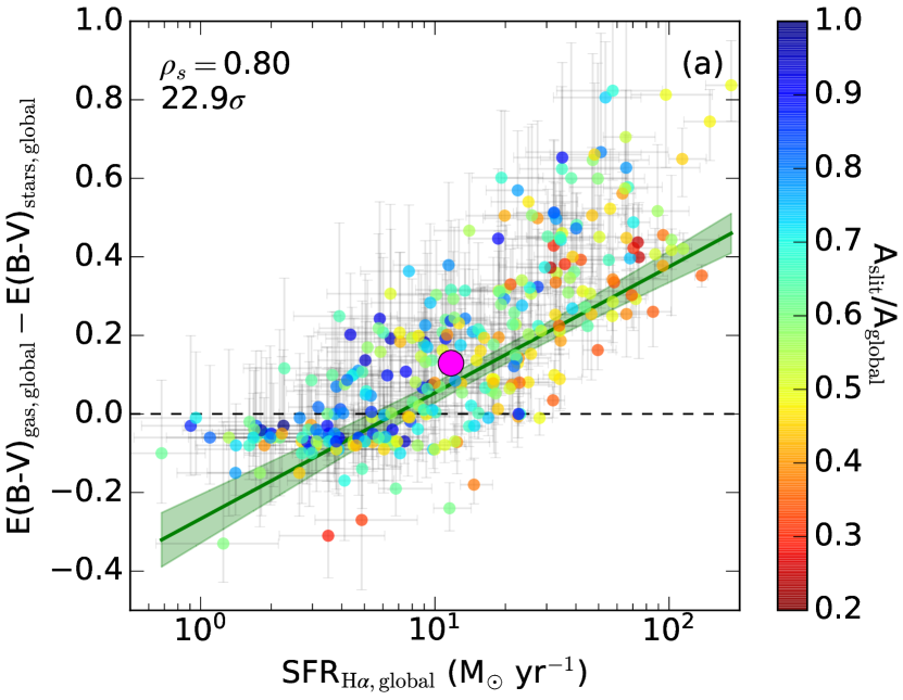
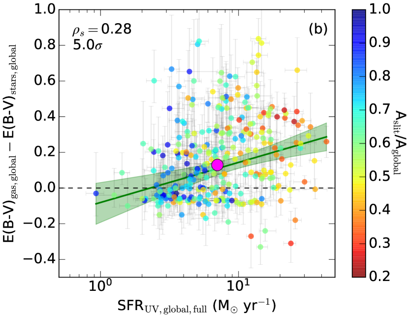
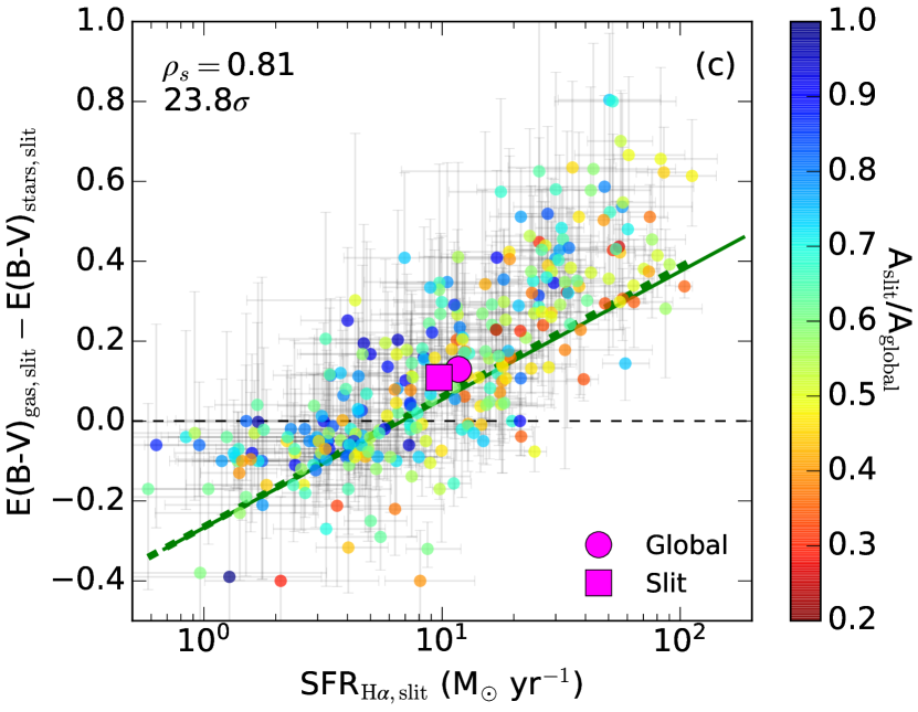
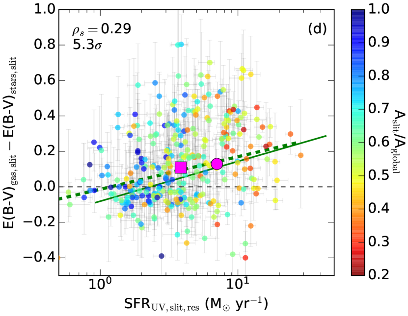
Figure 5: Differences between nebular and stellar continuum $E(B-V)$ versus SFR${}_{\text{H}\alpha}$ (left) and SFR${}_{\text{UV}}$ (right) for when all measurements are made globally (top) or exclusively within the spectroscopic slit area (bottom) for the 303 galaxies in the sample. The points are colored by the fraction of the galaxy that falls within the slit area (see Figure 2). The purple symbols show the median difference between $E(B-V)_{\text{gas}}$ and $E(B-V)_{\text{stars}}$ and the median SFR${}_{\text{H}\alpha}$ or SFR${}_{\text{UV}}$ for when measurements are made globally (circles) or directly within the slit area (squares). The horizontal black dashed lines shows where $E(B-V)_{\text{gas}}$ and $E(B-V)_{\text{stars}}$ are equal. The solid green lines show the best-fit linear relationship when all measurements are made globally and the dashed green lines show the best-fit linear relationship when all measurements are made directly within the slit region. The green shaded regions show the 3$\sigma$ confidence intervals of the best-fit linear relationships for the global measurements. The Spearman rank correlation coefficient and its significance are listed in the top left corner of each panel.

In Figure 3, the globally inferred nebular and stellar continuum reddening (left panels) and H$\alpha$ and UV SFRs (right panels) are compared to those derived exclusively from the flux in the spectroscopic slit area. The points are color-coded by the fraction of the galaxy falling in the slit, A${}_{\text{slit}}$/A${}_{\text{global}}$, where A${}_{\text{global}}$ is the are subsumed by the pixels that cover the surface area of the galaxy as identified by the segmentation map provided with the 3D-HST imaging, and A${}_{\text{slit}}$ is the area of the subset of pixels that cover the same area as the MOSFIRE spectroscopic slit. Therefore, small values of A${}_{\text{slit}}$/A${}_{\text{global}}$ represent physically large galaxies (red in color) and larger values of A${}_{\text{slit}}$/A${}_{\text{global}}$ approaching unity represent compact galaxies (blue in color). Panels (a) and (b) of Figure 3 compare the spectroscopic slit-based measurements with the global measurements, where the latter is inferred based on applying the slit-loss corrections discussed in Section 2.2.1. The $E(B-V)_{\text{gas}}$ determined from H$\alpha$ and H$\beta$ emission is assumed to apply over the entire galaxy, and the slit-loss corrections assume that the H$\alpha$ emission profile has the same shape as the optical light profile (i.e., $H_{160}$ image; see Section 2.2.1). As a result, the slit-measured nebular reddening, $E(B-V)_{\text{gas,slit}}$, is essentially identical to the global value, $E(B-V)_{\text{gas,global}}$ (panel a), with only small deviations being attributed to minor differences between the slit-loss corrections for H$\alpha$ and H$\beta$ caused by differences in seeing conditions of the observations of the relevant bands (see Section 2.2.1). Naturally, SFR${}_{\text{H}\alpha}$ measurements within the slit, SFR${}_{\text{H}\alpha\text{,slit}}$, are lower those measured globally, SFR${}_{\text{H}\alpha\text{,global}}$ (0.10 dex lower on average), where the difference depends on the fraction of the galaxy falling in the slit (A${}_{\text{slit}}$/A${}_{\text{global}}$; panel b). Panel (c) shows that the reddening of the stellar continuum measured from the 3D-HST photometry, $E(B-V)_{\text{stars,global}}$, is similar to that measured when only considering flux that falls in the slit, $E(B-V)_{\text{stars,slit}}$, for most galaxies. There are 29 galaxies with $E(B-V)_{\text{stars,slit}}$ that are $>$2$\sigma$ ($\sim$0.12 mag) redder (higher) than $E(B-V)_{\text{stars,global}}$, which can be attributed to the UV slope being poorly constrained by the resolved photometry (see Fetherolf et al., 2020). As discussed in Section 2.3, we required SFR${}_{\text{UV}}$ measured within the slit, SFR${}_{\text{UV,slit}}$, to be lower than SFR${}_{\text{UV}}$ measured globally, SFR${}_{\text{UV,global}}$, in order to be included in the sample. Panel (d) shows that SFR${}_{\text{UV,slit}}$ is on average 0.27 dex lower than SFR${}_{\text{UV,global}}$, and the size of the galaxy (i.e., A${}_{\text{slit}}$/A${}_{\text{global}}$) correlates more significantly with SFR${}_{\text{UV,global}}$ than the difference between slit and global SFR${}_{\text{UV}}$ measurements (see Section 4.4 for further discussion).

The SFR${}_{\text{UV,global}}$ shown in Figure 3d is derived using the extended wavelength coverage available through the photometry provided by the 3D-HST photometric catalog, and includes unresolved photometry from other ground- and space-based facilities. The SFR${}_{\text{UV,slit}}$, on the other hand, only utilizes the photometry with resolved CANDELS/3D-HST imaging and normalized IRAC photometry (see Section 3.1). In the left panel of Figure 4, these two methods for measuring SFR${}_{\text{UV,global}}$ are compared. The 121 galaxies with poorly constrained resolved photometry or with SFR${}_{\text{UV,slit}}$ measurements that are higher than SFR${}_{\text{UV,global}}$ (white empty points; see Section 3.2) are included to demonstrate that these “unphysical” measurements lie on the higher SFR side of the resultant scatter when SFR${}_{\text{UV}}$ are measured from fewer photometric points. It can be seen that SFR${}_{\text{UV}}$ measured from the 3D-HST photometric catalog agrees on average with those derived from only the resolved photometry (colored star symbol).

The right panel of Figure 4 is similar to Figure 3d, except that both SFR${}_{\text{UV,global}}$ and SFR${}_{\text{UV,slit}}$ are derived only using the resolved CANDELS/3D-HST and normalized IRAC photometry. The right panel of Figure 4 more clearly shows how the difference between SFR${}_{\text{UV,global}}$ and SFR${}_{\text{UV,slit}}$ changes with galaxy size (i.e., A${}_{\text{slit}}$/A${}_{\text{global}}$) and that SFR${}_{\text{UV,slit}}$ is 0.10 dex lower on average than SFR${}_{\text{UV,global}}$. As previously stated in Section 3.2, Fetherolf et al. (2020) showed that limited photometric coverage of the UV slope and other critical SED features (e.g., Balmer/4000 Å break) leads to redder $E(B-V)_{\text{stars}}$ and younger ages. While measurements for SFR${}_{\text{UV,slit}}$ can only utilize the wavebands with resolved imaging available (and normalized IRAC photometry), SFR${}_{\text{UV,global}}$ can be measured more robustly by using the data from several unresolved filters that is available in the 3D-HST photometric catalog. Furthermore, alternatively using the SFR${}_{\text{UV,global}}$ derived only from the resolved photometry—rather than all unresolved filters available through the 3D-HST photometric catalog—in the subsequent analysis does not significantly alter the primary conclusions of this paper. Therefore, for the remainder of the analysis we use the more reliable SFR${}_{\text{UV,global}}$ derived from the 3D-HST photometric catalog, which also has the benefit of being more comparable to other studies.

4.2 Difference in $E(B-V)$ vs. SFR

 

 

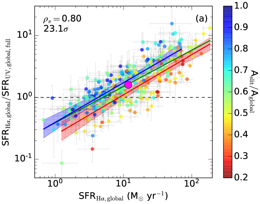
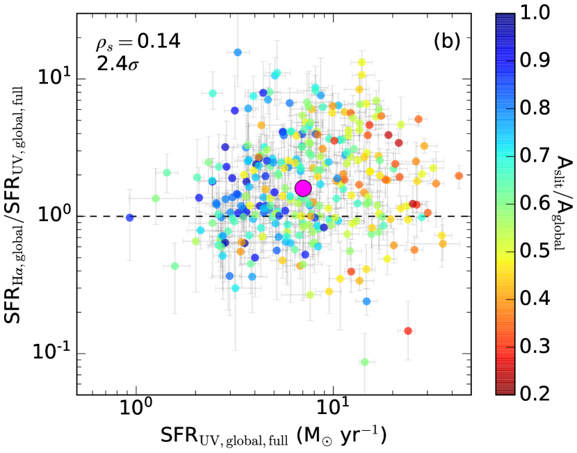
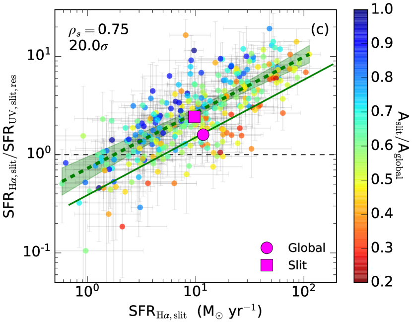
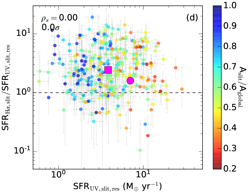
Figure 6: Top: Globally measured dust-corrected H$\alpha$-to-UV SFR ratios versus dust-corrected SFR${}_{\text{H}\alpha}$ (left) and SFR${}_{\text{UV}}$ (right) for the 303 galaxies in the sample. The black horizontal dashed line indicates where the SFR${}_{\text{H}\alpha}$ would equal SFR${}_{\text{UV}}$ and the points are colored by the fraction of the galaxy that falls within the slit area (see Figure 2). The solid lines show the best-fit relationships for the full sample (green), compact galaxies with $\mbox{A${}_{\text{slit}}$/A${}_{\text{global}}$}>0.6$ (blue), and large galaxies with $\mbox{A${}_{\text{slit}}$/A${}_{\text{global}}$}<0.6$ (red). The blue and red shaded regions show the 3$\sigma$ confidence intervals of the best-fit relationships of the compact and large galaxies, respectively, thus emphasizing how the offset from the relationship between H$\alpha$-to-UV SFR ratios and SFR${}_{\text{H}\alpha}$ is dependent on galaxy size. Bottom: Same as the top panels, except that all of the dust-corrected SFRs (and their respective inferred reddening) are measured exclusively within the spectroscopic slit area. The purple symbols show the median H$\alpha$-to-UV SFR ratio, SFR${}_{\text{H}\alpha}$, and SFR${}_{\text{UV}}$ for when measurements are made globally (circles) or directly within the slit area (squares). The dashed green lines shows the best-fit relationship to the full sample for the slit-measured SFRs and, for reference, the solid green lines show the best-fit relationship to the global measurements of the full sample from the top panels. The green shaded regions show the 3$\sigma$ confidence interval of the slit-measured best-fit relationships for all galaxies, thus emphasizing the significance of the shift in normalization between SFR measurements made exclusively within the slit area (bottom panels) compared to those made across the entire galaxy (top panels). The Spearman rank correlation coefficient and its significance are listed in the top left corner of each panel.

Figure 5 shows how the difference between nebular and stellar continuum reddening varies as a function of SFR, both when all properties are inferred from global flux measurements and when they are inferred from flux measurements restricted to the spectroscopic aperture. The Spearman rank correlation coefficient and the significance of the correlation is listed in the top left corner of each panel. The top panels show the difference between $E(B-V)_{\text{gas,global}}$ and $E(B-V)_{\text{stars,global}}$ versus SFR${}_{\text{H}\alpha\text{,global}}$ (panel a) and SFR${}_{\text{UV,global}}$ (panel b) when slit-loss corrections are applied to the emission line measurements and the SED is fit to the 3D-HST photometry covering the entire galaxy. The scipy.odr package is used to perform orthogonal distance regression linear fits and obtain 3$\sigma$ confidence intervals on the relationship between differences in reddening and SFR for the top panels of Figure 5 (solid green lines and shaded regions). The observed correlations are partially caused by the SFR being dust-corrected using $E(B-V)$. Specifically, the dust corrections cause SFR${}_{\text{H}\alpha}$ to be dependent on $E(B-V)_{\text{gas}}$ (see Section 3.3) and SFR${}_{\text{UV}}$ to be dependent on $E(B-V)_{\text{stars}}$. However, the reddening and SFR derived from the nebular emission ($E(B-V)_{\text{gas}}$ and SFR${}_{\text{H}\alpha}$) are independent from those derived from the UV continuum ($E(B-V)_{\text{stars}}$ and SFR${}_{\text{UV}}$) since they are measured separately from the spectroscopy and photometry, respectively. The bottom panels of Figure 5 show how the difference in $E(B-V)_{\text{gas,slit}}$ and $E(B-V)_{\text{stars,slit}}$ varies with SFR${}_{\text{H}\alpha\text{,slit}}$ (panel c) and SFR${}_{\text{UV,slit}}$ (panel d) when slit-loss corrections are not applied and the SED is only fit to the photometric flux with spectroscopic slit coverage (see Section 3.1). The best-fit linear relationships based on the reddening and SFRs derived globally (solid green lines) and exclusively within the slit (dashed green lines) are both shown in the bottom panels in order to demonstrate the changes between the top (global) and bottom (slit) panels. Figure 5 shows that the general relationship between the difference in reddening probes and SFR is statistically significant (23$\sigma$ for SFR${}_{\text{H}\alpha}$ and 5$\sigma$ for SFR${}_{\text{UV}}$) and persists regardless of whether measurements are made directly within the slit or inferred globally, suggesting that aperture effects have little impact on the significance of the correlation (see Section 5 for an in-depth discussion). In both cases $E(B-V)_{\text{gas}}$ is on average higher than $E(B-V)_{\text{stars}}$ (0.16 mag globally and 0.13 mag in the slit), with agreement at lower SFRs and a larger discrepancy at higher SFRs.

4.3 H$\alpha$-to-UV SFR Ratios

Figure 6 shows the relationship between H$\alpha$-to-UV SFR ratios versus SFR${}_{\text{H}\alpha}$ (left panels) and SFR${}_{\text{UV}}$ (right panels) when SFRs are either derived from the entire galaxy area (top panels) or exclusively within the spectroscopic slit area (bottom panels). As can be seen by the median H$\alpha$-to-UV SFR ratio (purple symbols), SFR${}_{\text{H}\alpha}$ is typically higher than SFR${}_{\text{UV}}$ (0.22 dex for global measurements and 0.39 dex within the slit). Furthermore, Figure 6 shows that SFR${}_{\text{H}\alpha}$ and SFR${}_{\text{UV}}$ tend to generally agree in galaxies with lower SFR${}_{\text{H}\alpha}$ and deviate more significantly as SFR${}_{\text{H}\alpha}$ increases. The persistence of the correlation between H$\alpha$-to-UV SFR ratios and SFR${}_{\text{H}\alpha}$ when all SFRs are measured inside the slit further implies that the trend is not induced by aperture effects. The solid and dashed lines in Figure 6 show the best-fit linear relationships between H$\alpha$-to-UV SFR ratios and SFR${}_{\text{H}\alpha}$ for the full sample (green), compact galaxies with $\mbox{A${}_{\text{slit}}$/A${}_{\text{global}}$}>0.6$ (blue), and large galaxies with $\mbox{A${}_{\text{slit}}$/A${}_{\text{global}}$}<0.6$ (red), where 0.6 is the average area fraction covered by the slit of all galaxies in the sample. To show how the relationship changes between the global and slit measurements, the best-fit relationship to the full sample from Figure 6a is also shown as a solid green line in panel (c). We find that the slope (panel c) and scatter between H$\alpha$-to-UV SFR ratios and either probe of SFR are approximately the same regardless of the area over which SFRs are measured (the scatter is 0.22 dex for global and 0.25 dex within the slit). The primary difference between global (top panels) and slit-measured (bottom panels) SFRs is the shift between the median points (purple) and, in particular, the shift in the normalization of the trend between H$\alpha$-to-UV SFR ratios and SFR${}_{\text{H}\alpha}$ (panel c; dashed green line compared to the solid green line). The shift in normalization is partly due to lower SFR within the slit region, but there is also an additional shift in the H$\alpha$-to-UV SFR ratio, which we further discuss in Section 5. Alternatively investigating the difference between nebular and stellar continuum reddening and H$\alpha$-to-UV SFR ratio versus stellar mass, $E(B-V)_{\text{gas}}$, or $E(B-V)_{\text{stars}}$ produces similar results due to the well-known SFR–$M_{*}$ relationship (see Figure 1) and since the dust-corrected SFR is dependent on $E(B-V)$ by definition, but with additional uncertainty for galaxies with low reddening when $E(B-V)$ is consistent with (and assumed to be) zero.

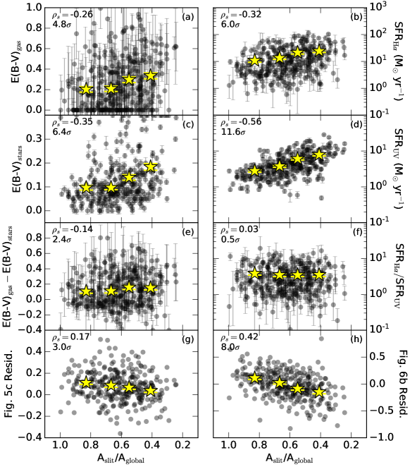
Figure 7: Correlations between the fraction of the galaxy within the slit area (i.e., galaxy size) and the following measurements that were all made directly within the slit area: nebular reddening (panel a), SFR${}_{\text{H}\alpha}$ (panel b), stellar continuum reddening (panel c), SFR${}_{\text{UV}}$ (panel d), the difference between nebular and stellar continuum reddening (panel e), H$\alpha$-to-UV SFR ratio (panel f), the residuals from the best-fit linear relation (dashed green line) shown in Figure 5c (panel g), and the residuals from the best-fit linear relation (dashed green line) shown in Figure 6b (panel h). Since compact galaxies have larger fractional slit areas (A${}_{\text{slit}}$/A${}_{\text{global}}$ $\approx 1$) than physically large galaxies, the x-axis labels have been reversed. The yellow stars are the averages from individual measurements equally divided into four bins of the fractional slit area (A${}_{\text{slit}}$/A${}_{\text{global}}$). The Spearman rank correlation coefficient and its significance are listed in the top left corner of each panel.

4.4 $E(B-V)$ and SFR vs. Size

In Figures 3 through 6, it can be seen that A${}_{\text{slit}}$/A${}_{\text{global}}$ (color-coded points; i.e., galaxy size) is correlated with various plotted quantities. In particular, the best-fit linear relationships shown in Figure 6a indicate that the normalization of the trend between H$\alpha$-to-UV SFR ratios and H$\alpha$ SFRs is dependent on size, where the blue and red linear fits represent compact and large galaxies, respectively. In this section we analyze the significance of galaxy size on the relationships discussed in Section 4.2 and Section 4.3 using the Spearman rank correlation test.

Figure 7 shows how A${}_{\text{slit}}$/A${}_{\text{global}}$ (i.e., galaxy size) correlates with $E(B-V)_{\text{gas,slit}}$ (panel a), SFR${}_{\text{H}\alpha\text{,slit}}$ (panel b), $E(B-V)_{\text{stars,slit}}$ (panel c), SFR${}_{\text{UV,slit}}$ (panel d), the difference between $E(B-V)_{\text{gas,slit}}$ and $E(B-V)_{\text{stars,slit}}$ (panel e), slit-measured H$\alpha$-to-UV SFR ratios (panel f), and the residuals from the best-fit linear relationships (dashed green lines) shown in Figure 5c and Figure 6c (panels g and h). All measurements in Figure 7 are made directly within the slit in order to avoid the added complexity to the interpretation when slit-loss correction assumptions are applied.

We find that light is more dust reddened in larger galaxies (lower A${}_{\text{slit}}$/A${}_{\text{global}}$; 5$\sigma$ for $E(B-V)_{\text{gas}}$ and 6$\sigma$ for $E(B-V)_{\text{stars}}$; panels a and c) and that larger galaxies have higher SFRs (6$\sigma$ for SFR${}_{\text{H}\alpha}$ and 12$\sigma$ for SFR${}_{\text{UV}}$; panels b and d) compared to compact galaxies. The two probes of dust reddening also tend to be more discrepant in larger galaxies, with nebular reddening being higher than that of the stellar continuum (2.4$\sigma$; panel e). At a fixed SFR${}_{\text{H}\alpha}$, on the other hand, compact galaxies tend to exhibit a more significant difference between nebular and stellar continuum reddening than large galaxies (3$\sigma$; panel g). However, the trend observed in panel (g) may be exaggerated since SFR${}_{\text{H}\alpha}$ depends on $E(B-V)_{\text{gas}}$ (see Section 5 for an in-depth discussion). Similarly, when considering that H$\alpha$-to-UV SFR ratios are generally insensitive to galaxy size (0.5$\sigma$; panel f) and that SFR${}_{\text{H}\alpha}$ is fixed for a range of H$\alpha$-to-UV SFR ratios in Figure 6b, it follows that the trend between galaxy sizes and the residuals between H$\alpha$-to-UV SFR ratios and SFR${}_{\text{H}\alpha}$ (8$\sigma$; panel h) is likely caused by the strong correlation between SFR${}_{\text{UV}}$ and galaxy size (12$\sigma$; panel d). Finally, we note that all of these correlations persist and become more significant when all measurements are alternatively made globally across the galaxy, again suggesting that these relationships are not caused by aperture effects.

5 Discussion

5.1 Aperture Effects

To interpret the results of our analysis, we first need to assess how the coverage of the spectroscopic slit with respect to the surface area of the galaxies influences the results. We consider A${}_{\text{slit}}$/A${}_{\text{global}}$ as a proxy for physical size of the galaxies in our sample since a given angular size corresponds to an approximately fixed physical size over the redshift range covered by our sample ($1.36<z<2.66$) and all galaxies are observed using a fixed 0$\aas@@fstack{\prime\prime}$7 slit width. To remind the reader, Figure 2 shows the observed and unobserved emission from a compact and large galaxy relative to the spectroscopic slit boundaries. Galaxies that are nearly entirely contained within the slit boundaries (i.e., the compact galaxies) have a A${}_{\text{slit}}$/A${}_{\text{global}}$ near unity, and thus the slit-measured $E(B-V)_{\text{gas}}$ and SFR${}_{\text{H}\alpha}$ of compact galaxies will be close to those that would be measured globally—if such measurements existed. Large galaxies with lower A${}_{\text{slit}}$/A${}_{\text{global}}$, on the other hand, require larger corrections for light lost outside of the slit area. The changes between slit-measured and globally inferred quantities for $E(B-V)_{\text{gas}}$ (Figure 3a) and SFR${}_{\text{H}\alpha}$ (Figure 3b) are influenced by the assumptions made when correcting for slit-loss. The usual assumptions when correcting for spectroscopic slit-loss is that the measured Balmer decrement (H$\alpha$/H$\beta$) is representative of the average nebular reddening across the galaxy and that the fraction of H$\alpha$ light lost outside the slit is equal to the fraction of $H_{160}$ light lost outside the slit. On the other hand, both the slit and global quantities for $E(B-V)_{\text{stars}}$ (Figure 3c) and SFR${}_{\text{UV}}$ (Figure 3d) can be directly measured from the resolved CANDELS/3D-HST photometry.

The top panels of Figure 5 show that $E(B-V)_{\text{gas,global}}$ and $E(B-V)_{\text{stars,global}}$ become more discrepant as the global SFR increases, and the top panels of Figure 6 show that SFR${}_{\text{H}\alpha\text{,global}}$ is higher than SFR${}_{\text{UV,global}}$, particularly in galaxies with higher SFR${}_{\text{H}\alpha\text{,global}}$ (panel a). These observations could be explained if the globally averaged $E(B-V)_{\text{gas}}$ or the total H$\alpha$ light is overestimated by the slit-loss corrections in galaxies with high SFRs. If the slit-loss corrections lead to overestimated $E(B-V)_{\text{gas}}$ and/or SFR${}_{\text{H}\alpha}$, then the trends observed in the top panels of Figure 5 and Figure 6a would not be present when the slit-loss corrections are not incorporated into the spectroscopic measurements. However, the slit-measured quantities shown in the bottom panels of Figure 5 and Figure 6 show that there is no significant change in the significance or slope of these relationships. The $E(B-V)_{\text{gas}}$ is larger than $E(B-V)_{\text{stars}}$ at high SFRs, and SFR${}_{\text{H}\alpha}$ remains higher than SFR${}_{\text{UV}}$ at high SFR${}_{\text{H}\alpha}$. Furthermore, at a fixed SFR${}_{\text{H}\alpha}$ we found a systematic shift towards lower differences between $E(B-V)_{\text{gas}}$ and $E(B-V)_{\text{stars}}$, and lower H$\alpha$-to-UV SFR ratios for larger galaxies. Therefore, we conclude that these relationships must reflect the physical properties of the galaxies in our sample.

The best-fit linear relationships included in the bottom panels of Figure 5 and Figure 6c are used to compare the changes between when all quantities are either inferred globally (solid green lines) or measured directly within the slit area (dashed green lines). If $E(B-V)_{\text{gas}}$, $E(B-V)_{\text{stars}}$, and the H$\alpha$-to-UV SFR ratio are equivalent within the slit area and globally across the entire galaxy—which is the assumed behavior when estimating the slit-loss corrections that are described in Section 2.2.1—then in all cases these best-fit linear relationships are expected to shift towards lower H$\alpha$ and UV SFR by definition when the slit-loss corrections are reversed ($\mbox{SFR${}_{\text{slit}}$}<\mbox{SFR${}_{\text{global}}$}$; solid to dashed green lines; also see right panels of Figure 3). By comparing the solid and dashed green lines in the bottom panels of Figure 5, it can be seen that there is no significant change in the slope or normalization of the relationship between the difference in reddening probes versus SFR. By comparing the median of the sample when all measurements are made globally (purple circles) versus exclusively inside the slit (purple squares), it can be seen that there is a shift towards lower SFR${}_{\text{H}\alpha}$ (as expected) and lower $\mbox{$E(B-V)_{\text{gas}}$}-\mbox{$E(B-V)_{\text{stars}}$}$ that causes the two relationships to exhibit a similar slope and normalization. The shift towards lower $\mbox{$E(B-V)_{\text{gas}}$}-\mbox{$E(B-V)_{\text{stars}}$}$ is caused by the 29 galaxies that are $>$2$\sigma$ redder (higher) in $E(B-V)_{\text{stars,slit}}$ than their $E(B-V)_{\text{stars,global}}$ (Figure 3c), which essentially cancels the shift towards lower SFRs. Figure 6c shows no significant change in the slope of the relationship between H$\alpha$-to-UV SFR ratios and SFR${}_{\text{H}\alpha}$, but there is a significant shift in the normalization of the best-fit linear relationship towards lower SFRs and higher H$\alpha$-to-UV SFR ratios when all measurements are made within the slit compared to those measured globally. In this case, in addition to the leftwards shift caused by SFR${}_{\text{H}\alpha\text{,slit}}$ being less than SFR${}_{\text{H}\alpha\text{,global}}$, the median points also show a significant shift towards higher H$\alpha$-to-UV SFR ratios. This significant normalization shift towards higher H$\alpha$-to-UV SFR ratios is caused by the relative change between global and slit-measured SFRs not being equivalent between SFR${}_{\text{H}\alpha}$ and SFR${}_{\text{UV}}$ (0.10 dex and 0.27 dex, respectively; see right panels of Figure 3), as is assumed for constant H$\alpha$-to-UV SFR ratios in the slit-loss corrections, and could possibly be indicative of differences between the H$\alpha$ and UV light profiles in these galaxies (see Section 5.3 for further discussion). The observed normalization shift in Figure 6c is less significant when SFR${}_{\text{UV,global}}$ is alternatively derived exclusively from the resolved CANDELS/3D-HST photometry (Figure 4) since these measurements are typically only 0.10 dex higher than SFR${}_{\text{UV,slit}}$, but the observed normalization offset towards higher H$\alpha$-to-UV SFR ratios is still significant by $>$3$\sigma$ for $\mbox{SFR${}_{\text{H}\alpha}$}\gtrsim 2$ $M_{\odot}$ yr^-1 (see right panel of Figure 4).

5.2 Differences between $E(B-V)_{\text{gas}}$ and $E(B-V)_{\text{stars}}$

The bottom panels of Figure 5 show that the observed differences between $E(B-V)_{\text{gas}}$ and $E(B-V)_{\text{stars}}$ persist in galaxies with higher SFR${}_{\text{H}\alpha}$ (panel c) and SFR${}_{\text{UV}}$ (panel d), even when all measurements are made exclusively within the spectroscopic slit area. The increasing difference between nebular and stellar continuum $E(B-V)$ with SFR may imply that the dust distribution is patchier in galaxies with higher SFRs (which are also inherently dustier; Calzetti et al., 1994; Boquien et al., 2009; Price et al., 2014; Reddy et al., 2015), such that the nebular emission becomes dominated by the most obscured massive stars. However, SFR${}_{\text{H}\alpha}$ and SFR${}_{\text{UV}}$ are not independent from $E(B-V)_{\text{gas}}$ or $E(B-V)_{\text{stars}}$, in that they are each used to correct these SFR indicators for the effects of dust. Therefore, the observed trends between the $E(B-V)$ difference and SFR in Figure 5, and similarly the trends observed in panels (e) and (g) of Figure 7 (due to the significant correlation between A${}_{\text{slit}}$/A${}_{\text{global}}$ and SFR${}_{\text{UV}}$ shown in panel d), may be exaggerated rather than being caused by the intrinsic characteristics of these galaxies. Furthermore, Shivaei et al. (2020) found that the relationship between the differences in $E(B-V)$ versus SFR (H$\alpha$ and UV) for $z\sim 2$ star-forming galaxies in the MOSDEF sample is less significant when the UV light is corrected using a metallicity-dependent dust attenuation curve. Therefore, understanding the nature of the difference between nebular and stellar continuum reddening would be best addressed using a SFR indicator that is independent from $E(B-V)_{\text{gas}}$ and $E(B-V)_{\text{stars}}$, such as total SFRs computed by combining unobscured UV and IR continuum measurements.

5.3 Variations in H$\alpha$-to-UV SFR Ratios

Figure 6c shows that the relationship between H$\alpha$-to-UV SFR ratios and SFR${}_{\text{H}\alpha}$ persists when all reddening and dust-corrected SFRs measurements are made directly inside the spectroscopic slit area, implying that the trend between H$\alpha$-to-UV SFR ratios and SFR${}_{\text{H}\alpha}$ is not driven by the slit-loss corrections. Furthermore, the offset of individual galaxies from the best-fit linear relation between H$\alpha$-to-UV SFR ratios and SFR${}_{\text{H}\alpha}$ (green lines) is significantly correlated with the fraction of the galaxy that is directly observed within the spectroscopic slit area (i.e., galaxy size; see Figure 2 and Figure 7h). By separately identifying the significance of the correlations between galaxy size and slit-measured SFR${}_{\text{H}\alpha}$, SFR${}_{\text{UV}}$, H$\alpha$-to-UV SFR, and the residuals from the best-fit relationship between H$\alpha$-to-UV SFR ratios versus SFR${}_{\text{H}\alpha}$ (right panels of Figure 7), we find that SFR${}_{\text{UV}}$ is most significantly correlated with galaxy size (panel d) and that H$\alpha$-to-UV SFR ratios are generally constant with galaxy size but with large scatter (panel f). It is well-known that larger galaxies tend to have higher SFRs on average compared to compact galaxies (panels b and d of Figure 7; Toft et al., 2007; Trujillo et al., 2007; van der Wel et al., 2014; Scott et al., 2017; van de Sande et al., 2018). However, further taking into account that the correlation between galaxy size and SFR is stronger in the UV than H$\alpha$, then it is expected by definition that, at a fixed size (or SFR${}_{\text{UV}}$) the H$\alpha$-to-UV SFR ratio will be higher for galaxies with higher SFR${}_{\text{H}\alpha}$ relative to galaxies with lower SFR${}_{\text{H}\alpha}$ at the same size (blue, green, and red lines in Figure 6a). Therefore, we reiterate how understanding the differences between H$\alpha$ and UV SFRs would be best addressed using independently derived galaxy properties, such as SFRs measured from the far-IR continuum.

Generally, the H$\alpha$-to-UV SFR ratio may reflect variations in the SFHs of galaxies (Reddy et al., 2012b; Price et al., 2014; Madau & Dickinson, 2014). High H$\alpha$-to-UV SFR ratios, which we observe in galaxies with SFRs $\gtrsim$2 $M_{\odot}$ yr^-1, could be indicative of SFRs that change on timescales $<$100 Myr. However, a single rapid burst, or galaxies with complex SFHs, may not sufficiently affect the H$\alpha$-to-UV luminosities in order to explain the observed SFR discrepancies (e.g., Emami et al., 2019). Furthermore, observations of local galaxies have found that bursty star formation is more typical of low-mass dwarf galaxies ($<$10⁹ $M_{\odot}$; Weisz et al., 2012; Guo et al., 2016; Emami et al., 2019), which are lower in mass than the majority of the galaxies in our sample. We find better agreement between SFR${}_{\text{H}\alpha}$ and SFR${}_{\text{UV}}$ for galaxies with lower SFRs, which corresponds with the lowest mass galaxies in our sample (Figure 1). Figure 7f suggests that H$\alpha$-to-UV SFR ratios measured from compact galaxies are consistent with those measured from the centers of large galaxies, such that H$\alpha$-to-UV SFR ratios may not be correlated with the physical sizes of galaxies. On the other hand, H$\alpha$ and UV light profiles may not necessarily follow each other in the outskirts of large galaxies, which are beyond the capability of the MOSDEF observations used in the current study (without making assumptions for spectroscopic slit-loss). Centrally peaked H$\alpha$ and Balmer decrement radial profiles have been observed in galaxies at $1<z<3$ using resolved emission line maps (e.g., Nelson et al., 2013; Hemmati et al., 2015; Tacchella et al., 2018). Furthermore, massive star-forming galaxies, which are well-known to be larger (e.g., Toft et al., 2007; Trujillo et al., 2007; van der Wel et al., 2014; Tacchella et al., 2015; Scott et al., 2017; Isobe et al., 2020), dustier (e.g., Reddy et al., 2006, 2010; Pannella et al., 2009; Price et al., 2014; Shivaei et al., 2020), and have higher SFRs (e.g., Noeske et al., 2007; Daddi et al., 2007; Pannella et al., 2009; Wuyts et al., 2011; Reddy et al., 2012b; Whitaker et al., 2012; Whitaker et al., 2014; Shivaei et al., 2015b) than low-mass galaxies on average, exhibit stronger centrally peaked H$\alpha$ and Balmer decrement radial profiles than low-mass galaxies (Nelson et al., 2016). If the H$\alpha$ emission is centrally peaked in a galaxy relative to its $H_{160}$ light profile, then the typical assumptions when correcting for slit loss may result in overestimated SFR${}_{\text{H}\alpha}$. In the MOSDEF survey, we can only observe a small fraction of the surface area of large galaxies spectroscopically (see Figure 2). However, it is possible that these large galaxies have higher SFR${}_{\text{H}\alpha}$ in their centers compared to their unobserved outskirts (normalization shift between the green lines in Figure 6c), which could be indicative of inside-out galaxy growth (e.g., Patel et al., 2013; Gomes et al., 2016; Nelson et al., 2016; Jafariyazani et al., 2019). Similarly, if Balmer decrements are typically higher in the centers of large galaxies compared to their outskirts, then the assumed average reddening based on the slit measurements will overestimate the globally-averaged reddening.

Deviations in the attenuation curve relative to the one assumed can cause large systematic uncertainties such that derivations of certain stellar population properties may require more realistic attenuation curves for high-redshift galaxies, such as a mass or metallicity dependent attenuation curve (e.g., Reddy et al., 2006, 2010, 2012a, 2018; Noll et al., 2009; Siana et al., 2009; Kriek & Conroy, 2013; Shivaei et al., 2018, 2020). Reddy et al. (2018) found that alternatively assuming a Calzetti et al. (2000) attenuation curve over an SMC extinction curve (Fitzpatrick & Massa, 1990; Gordon et al., 2003) causes a systematic shift in absolute masses—but not their relative order—and that assuming an SMC attenuation curve and sub-Solar metallicities is generally more appropriate for young, high-redshift galaxies, such as those in our sample (see Section 3.2). We consider variations in the dust-to-star geometry relative to that which is already assumed by the choice of attenuation curve that could explain the observed discrepancies between inferred $E(B-V)$ and dust-corrected SFRs. The increase in H$\alpha$-to-UV SFR ratios with SFR, for example, may be a result of a patchier distribution of dust in galaxies with higher SFRs. In this scenario, stars of all masses are obscured by roughly the same columns of dust at low SFR, while the younger stellar populations will generally be more obscured in higher SFR galaxies (e.g., Reddy et al., 2015). However, a patchy dust distribution could also cause some sightlines towards older OB associations that contribute to the nebular emission to be less obscured than those still enshrouded by their birth clouds. Galaxies with patchier dust distributions (or centrally peaked SFR${}_{\text{H}\alpha}$ and/or Balmer decrements) may also exhibit H$\alpha$ and UV light profiles that do not match at all radii in large galaxies. Inappropriate assumptions about the shape of the H$\alpha$ and UV light profiles relative to each other may explain: 1) the normalization shift between H$\alpha$-to-UV SFR ratios that is observed inside the slit compared to global measurements (Figure 6c), and 2) the correlation between the size of a galaxy and the scatter in the relationship between H$\alpha$-to-UV SFR ratios and SFR${}_{\text{H}\alpha}$ (Figure 7h). We will further explore the distribution of dust and its relationship to globally measured properties of the $z\sim 2$ MOSDEF galaxies in a future work by performing an in-depth analysis of the reddening maps created through the procedures described in Fetherolf et al. (2020).

6 Summary

In this study, we used a sample of 303 star-forming galaxies drawn from the MOSDEF survey at spectroscopic redshifts $1.36<z<2.66$ in order to directly compare nebular and stellar continuum dust reddening, and dust-corrected SFRs measured from H$\alpha$ emission and the UV continuum light. We used the CANDELS/3D-HST high-resolution, multi-band imaging to measure the stellar population and dust properties both globally and within the MOSFIRE slit region. By combining the slit-measured stellar population and dust properties from the resolved imaging with the MOSDEF H$\alpha$ and H$\beta$ emission line measurements, we were able to directly obtain measurements of $E(B-V)_{\text{gas}}$, $E(B-V)_{\text{stars}}$, SFR${}_{\text{H}\alpha}$, and SFR${}_{\text{UV}}$ exclusively inside the MOSFIRE spectroscopic slit area.

In order to directly compare photometric and spectroscopic measurements over the same area, the HST imaging was PSF-smoothed to match the spatial resolution (i.e., seeing) of the MOSFIRE spectroscopic observations (Section 3.1). By directly comparing $E(B-V)$ and SFR measurements within the spectroscopic slit area, we found that aperture corrections alone cannot explain the observed differences between H$\alpha$ and UV probes of reddening and SFR that are most discrepant in galaxies with high SFR (Figure 5 and Figure 6). We also found that the offset from the best-fit linear relationship between H$\alpha$-to-UV SFR ratios and SFR${}_{\text{H}\alpha}$ is significantly correlated with galaxy size (Figure 6a and Figure 7h), but could be attributed to a stronger correlation between galaxy size and SFR${}_{\text{UV}}$ compared to SFR${}_{\text{H}\alpha}$ (panels b and d of Figure 7). Furthermore, the shift in normalization in the relationship between H$\alpha$-to-UV SFR ratios and SFR${}_{\text{H}\alpha}$ when all measurements are made directly within the slit compared to those made globally (Figure 6c) suggests that SFR${}_{\text{H}\alpha}$ may be higher in the centers of large galaxies compared to their outskirts. Assuming that the slit-loss corrections are adequate, higher SFR${}_{\text{H}\alpha}$ in the centers of large galaxies (where there is spectroscopic slit coverage) compared to their outskirts could be suggestive of inside-out galaxy growth.

To explain the observations presented in Section 4, we reiterate the physical scenario depicted by Reddy et al. (2015) where the dust distribution gets patchier as a function of increasing SFR. In this scenario the optical depth is on average higher in high-SFR galaxies, but the emitted light is dominated by young, massive stellar populations that may be less obscured than what is implied by the average measured reddening—thus leading to the discrepancy between H$\alpha$ and UV SFRs. Furthermore, large galaxies with higher SFRs may exhibit centrally peaked H$\alpha$ or Balmer decrement profiles (e.g., Nelson et al., 2013; Hemmati et al., 2015; Tacchella et al., 2018) such that their relative H$\alpha$ and UV light profiles are not necessarily equivalent at all radii.

Due to the nature of the MOSFIRE spectrograph, we can only draw direct conclusions based on the observations that fall within the slit area. Even with our limited spectroscopic capabilities, we see evidence that the observed discrepancies in $E(B-V)$ and SFRs measured from the nebular emission and the stellar continuum are caused by some physical driver—such as centrally peaked or patchy dust distributions—rather than systematic errors in the aperture corrections. These results can be improved upon with independent confirmation of the slit-loss corrections through IFU observations, high spatial resolution spectroscopy that could be used to compare H$\alpha$ and UV emission on smaller scales and out to larger radii, and pairing this analysis with a third independent SFR indicator (e.g., measured from the far-IR continuum). In direct follow-up to this work, we will investigate how the distribution of dust influences the observed SFRs and other globally measured physical properties of high-redshift galaxies.

Data Availability

Resolved CANDELS/3D-HST photometry is available at https://3dhst.research.yale.edu/Data.php. Spectroscopic redshifts, 1D spectra, and 2D spectra from the MOSDEF survey are available at http://mosdef.astro.berkeley.edu/for-scientists/data-releases/.

References

- Astropy Collaboration et al. (2013) Astropy Collaboration et al., 2013, A&A, 558, A33
- Astropy Collaboration et al. (2018) Astropy Collaboration et al., 2018, AJ, 156, 123
- Azadi et al. (2017) Azadi M., et al., 2017, ApJ, 835, 27
- Azadi et al. (2018) Azadi M., et al., 2018, ApJ, 866, 63
- Bertin & Arnouts (1996) Bertin E., Arnouts S., 1996, A&AS, 117, 393
- Boquien et al. (2009) Boquien M., et al., 2009, ApJ, 706, 553
- Boquien et al. (2015) Boquien M., et al., 2015, A&A, 578, A8
- Brammer et al. (2012) Brammer G. B., et al., 2012, ApJS, 200, 13
- Brinchmann et al. (2004) Brinchmann J., Charlot S., White S. D. M., Tremonti C., Kauffmann G., Heckman T., Brinkmann J., 2004, MNRAS, 351, 1151
- Bruzual & Charlot (2003) Bruzual G., Charlot S., 2003, MNRAS, 344, 1000
- Calzetti et al. (1994) Calzetti D., Kinney A. L., Storchi-Bergmann T., 1994, ApJ, 429, 582
- Calzetti et al. (2000) Calzetti D., Armus L., Bohlin R. C., Kinney A. L., Koornneef J., Storchi-Bergmann T., 2000, ApJ, 533, 682
- Cardelli et al. (1989) Cardelli J. A., Clayton G. C., Mathis J. S., 1989, ApJ, 345, 245
- Chabrier (2003) Chabrier G., 2003, PASP, 115, 763
- Coil et al. (2015) Coil A. L., et al., 2015, ApJ, 801, 35
- Daddi et al. (2007) Daddi E., et al., 2007, ApJ, 670, 156
- Emami et al. (2019) Emami N., Siana B., Weisz D. R., Johnson B. D., Ma X., El-Badry K., 2019, ApJ, 881, 71
- Erb et al. (2006) Erb D. K., Shapley A. E., Pettini M., Steidel C. C., Reddy N. A., Adelberger K. L., 2006, ApJ, 644, 813
- Faisst et al. (2017) Faisst A. L., et al., 2017, ApJ, 847, 21
- Fetherolf et al. (2020) Fetherolf T., et al., 2020, MNRAS, 498, 5009
- Fitzpatrick & Massa (1990) Fitzpatrick E. L., Massa D., 1990, ApJS, 72, 163
- Gomes et al. (2016) Gomes J. M., et al., 2016, A&A, 586, A22
- Gordon et al. (2003) Gordon K. D., Clayton G. C., Misselt K. A., Landolt A. U., Wolff M. J., 2003, ApJ, 594, 279
- Green et al. (2017) Green A. W., Glazebrook K., Gilbank D. G., McGregor P. J., Damjanov I., Abraham R. G., Sharp R., 2017, MNRAS, 470, 639
- Grogin et al. (2011) Grogin N. A., et al., 2011, ApJS, 197, 35
- Guo et al. (2016) Guo Y., et al., 2016, ApJ, 833, 37
- Hao et al. (2011) Hao C.-N., Kennicutt R. C., Johnson B. D., Calzetti D., Dale D. A., Moustakas J., 2011, ApJ, 741, 124
- Hemmati et al. (2015) Hemmati S., Mobasher B., Darvish B., Nayyeri H., Sobral D., Miller S., 2015, ApJ, 814, 46
- Hunter (2007) Hunter J. D., 2007, Computing in Science & Engineering, 9, 90
- Isobe et al. (2020) Isobe Y., et al., 2020, arXiv e-prints, p. arXiv:2004.11444
- Jafariyazani et al. (2019) Jafariyazani M., Mobasher B., Hemmati S., Fetherolf T., Khostovan A. A., Chartab N., 2019, ApJ, 887, 204
- Kashino et al. (2013) Kashino D., et al., 2013, ApJ, 777, L8
- Katsianis et al. (2017) Katsianis A., et al., 2017, MNRAS, 472, 919
- Kennicutt (1998) Kennicutt Jr. R. C., 1998, ARA&A, 36, 189
- Kennicutt & Evans (2012) Kennicutt R. C., Evans N. J., 2012, ARA&A, 50, 531
- Kewley et al. (2005) Kewley L. J., Jansen R. A., Geller M. J., 2005, PASP, 117, 227
- Koekemoer et al. (2011) Koekemoer A. M., et al., 2011, ApJS, 197, 36
- Kreckel et al. (2013) Kreckel K., et al., 2013, ApJ, 771, 62
- Kriek & Conroy (2013) Kriek M., Conroy C., 2013, ApJ, 775, L16
- Kriek et al. (2015) Kriek M., et al., 2015, ApJS, 218, 15
- Leung et al. (2019) Leung G. C. K., et al., 2019, ApJ, 886, 11
- Madau & Dickinson (2014) Madau P., Dickinson M., 2014, ARA&A, 52, 415
- McLean et al. (2010) McLean I. S., et al., 2010, in Ground-based and Airborne Instrumentation for Astronomy III. Proceedings of the SPIE, p. 77351E, doi:10.1117/12.856715, http://adsabs.harvard.edu/abs/2010SPIE.7735E..1EM
- McLean et al. (2012) McLean I. S., et al., 2012, in Ground-based and Airborne Instrumentation for Astronomy IV. p. 84460J, doi:10.1117/12.924794, http://adsabs.harvard.edu/abs/2012SPIE.8446E..0JM
- Meurer et al. (1999) Meurer G. R., Heckman T. M., Calzetti D., 1999, ApJ, 521, 64
- Momcheva et al. (2016) Momcheva I. G., et al., 2016, ApJS, 225, 27
- Narayanan et al. (2018) Narayanan D., Davé R., Johnson B. D., Thompson R., Conroy C., Geach J., 2018, MNRAS, 474, 1718
- Nelson et al. (2013) Nelson E. J., et al., 2013, ApJ, 763, L16
- Nelson et al. (2016) Nelson E. J., et al., 2016, ApJ, 817, L9
- Noeske et al. (2007) Noeske K. G., et al., 2007, ApJL, 660, L43
- Noll et al. (2009) Noll S., et al., 2009, A&A, 499, 69
- Oke & Gunn (1983) Oke J. B., Gunn J. E., 1983, ApJ, 266, 713
- Oliphant (2007) Oliphant T. E., 2007, Computing in Science & Engineering, 9, 10
- Osterbrock (1989) Osterbrock D. E., 1989, Astrophysics of gaseous nebulae and active galactic nuclei. John Simon Guggenheim Memorial Foundation, University of Minnesota, et al. Mill Valley, CA, University Science Books
- Pannella et al. (2009) Pannella M., et al., 2009, ApJL, 698, L116
- Patel et al. (2013) Patel S. G., et al., 2013, ApJ, 766, 15
- Price et al. (2014) Price S. H., et al., 2014, ApJ, 788, 86
- Reddy et al. (2006) Reddy N. A., Steidel C. C., Fadda D., Yan L., Pettini M., Shapley A. E., Erb D. K., Adelberger K. L., 2006, ApJ, 644, 792
- Reddy et al. (2010) Reddy N. A., Erb D. K., Pettini M., Steidel C. C., Shapley A. E., 2010, ApJ, 712, 1070
- Reddy et al. (2012a) Reddy N., et al., 2012a, ApJ, 744, 154
- Reddy et al. (2012b) Reddy N. A., Pettini M., Steidel C. C., Shapley A. E., Erb D. K., Law D. R., 2012b, ApJ, 754, 25
- Reddy et al. (2015) Reddy N. A., et al., 2015, ApJ, 806, 259
- Reddy et al. (2018) Reddy N. A., et al., 2018, ApJ, 853, 56
- Reddy et al. (2020) Reddy N. A., et al., 2020, ApJ, 902, 123
- Richards et al. (2016) Richards S. N., et al., 2016, MNRAS, 455, 2826
- Salim et al. (2007) Salim S., et al., 2007, ApJS, 173, 267
- Sanders et al. (2018) Sanders R. L., et al., 2018, ApJ, 858, 99
- Scott et al. (2017) Scott N., et al., 2017, MNRAS, 472, 2833
- Shivaei et al. (2015a) Shivaei I., Reddy N. A., Steidel C. C., Shapley A. E., 2015a, ApJ, 804, 149
- Shivaei et al. (2015b) Shivaei I., et al., 2015b, ApJ, 815, 98
- Shivaei et al. (2018) Shivaei I., et al., 2018, ApJ, 855, 42
- Shivaei et al. (2020) Shivaei I., et al., 2020, ApJ, 899, 117
- Siana et al. (2009) Siana B., et al., 2009, ApJ, 698, 1273
- Skelton et al. (2014) Skelton R. E., et al., 2014, ApJS, 214, 24
- Steidel et al. (2014) Steidel C. C., et al., 2014, ApJ, 795, 165
- Tacchella et al. (2015) Tacchella S., et al., 2015, ApJ, 802, 101
- Tacchella et al. (2018) Tacchella S., et al., 2018, ApJ, 859, 56
- Theios et al. (2019) Theios R. L., Steidel C. C., Strom A. L., Rudie G. C., Trainor R. F., Reddy N. A., 2019, ApJ, 871, 128
- Toft et al. (2007) Toft S., et al., 2007, ApJ, 671, 285
- Trujillo et al. (2007) Trujillo I., Conselice C. J., Bundy K., Cooper M. C., Eisenhardt P., Ellis R. S., 2007, MNRAS, 382, 109
- Weisz et al. (2012) Weisz D. R., et al., 2012, ApJ, 744, 44
- Whitaker et al. (2012) Whitaker K. E., van Dokkum P. G., Brammer G., Franx M., 2012, ApJL, 754, L29
- Whitaker et al. (2014) Whitaker K. E., et al., 2014, ApJ, 795, 104
- Wild et al. (2011) Wild V., Charlot S., Brinchmann J., Heckman T., Vince O., Pacifici C., Chevallard J., 2011, MNRAS, 417, 1760
- Wuyts et al. (2011) Wuyts S., et al., 2011, ApJ, 738, 106
- Wuyts et al. (2013) Wuyts S., et al., 2013, ApJ, 779, 135
- Yoshikawa et al. (2010) Yoshikawa T., et al., 2010, ApJ, 718, 112
- van de Sande et al. (2018) van de Sande J., et al., 2018, Nature Astronomy, 2, 483
- van der Wel et al. (2014) van der Wel A., et al., 2014, ApJ, 788, 28