Abstract

We propose an algebraic construction of the operator-state correspondence in non-relativistic conformal field theories by explicitly constructing an automorphism of the Schrödinger algebra relating generators in different frames. It is shown that the construction follows closely that of relativistic conformal field theories.

1 Introduction

The non-relativistic conformal group is the symmetry group of the free Schrödinger equation. On top of the Galilei subgroup, it includes non-relativistic dilatations and one special conformal transformation. Theories invariant under the (centrally extended) Schrödinger group are called non-relativistic conformal field theories (NRCFTs). Examples of those are non-relativistic particles with an $r^{-2}$ potential interaction and fermions at unitarity [1, 2, 3].

The name NRCFT can be somewhat misleading, for it evokes conformal field theory (CFT) suggesting that the former is a special case of the latter. However, NRCFT is only (if at all) a distant cousin of CFT. The Schrödinger group cannot be obtained (at least in the same number of dimensions [3]) from the conformal group by considering the non-relativistic limit. In other words, the relation between the two groups is not the same as between the Poincaré and Galilei groups, where the latter is the Inönü-Wigner contraction of the former.

Even putting aside the central charge $Q$ corresponding to the particle number in non-relativistic theory, the number of generators for the two groups is different: CFT has as many special conformal generators as the number of space-time dimensions, while in NRCFT there is only one analogue of the special conformal transformation, irrespectively of the spacetime dimensionality. Dilatations are also different in the two theories, since in CFT these do not distinguish between space and time, while in NRCFT time and spatial coordinates scale differently; this in turn allows to have dimensionful parameters, such as mass, clearly forbidden in CFT.

From an effective field theory perspective, the symmetry group of NRCFT is an accident of the non-relativistic limit. Considering higher order (in inverse powers of the speed of light) operators would bring in symmetry-breaking terms revealing that NRCFT originates from a Poincaré invariant theory rather than from a theory with an enhanced symmetry like a CFT.

Despite all the differences there are common features of conformal field theories and their non-relativistic counterparts, allowing to draw general conclusions about the two types of theories. For instance, the operators in both theories are organized into primaries and descendants and the operator product expansions (OPE) are determined by the corresponding contributions from primary operators. It can be shown [5, 6] that in both theories OPE has a finite radius of convergence and, which is intimately related to this fact, that both types of theories posses what is called an operator-state correspondence. The latter establishes a one-to-one map between states in the Hilbert space and the operators of a theory. In particular, the scaling dimensions of the operators are given by the energies of the corresponding states. One of the consequences of the operator-state correspondence is the presence of unitarity bounds on the scaling dimensions.

The fact that OPE converges also implies that higher order correlators can be expressed in terms of two point functions by applying the OPE repeatedly, in the same manner as in CFTs. However, developing a bootstrap program for NRCFT is complicated by the fact that three point functions are not fixed completely by kinematics only, as opposed to CFT (see [6] for more details).

Our main objective in this paper is to put forward an algebraic construction of the operator-state correspondence for NRCFTs, which parallels the procedure used when studying CFTs. Specifically, we discuss how the Hilbert space structure is introduced on the space of Euclidean fields. This is achieved by finding an automorphism relating the Minkowski and Euclidean generators of the conformal group. This way, the operator-state map is a natural aftermath of the proposed construction.

This work is organized as follows. In Sec. 2 we set the stage by rephrasing some well known results of CFTs in a language which can be used almost verbatim in the NRCFTs. We first give a brief overview of some basics about the conformal algebra and its unitary representations. Then, we turn to the operator-state correspondence and how this emerges as a consequence of the mapping between the Minkowski and Euclidean generators of the conformal algebra and the operator algebra. Sec. 3 is devoted to NRCFTs. Namely, we introduce the Schrödinger group and discuss the algebra’s representations and action on operators. Then, we construct the appropriate map between the generators of the algebra by finding the corresponding coordinate transformation. Finally, we explicitly demonstrate that in the non-relativistic considerations, confining the theory in a harmonic trap is completely analogous to putting a CFT on the cylinder. We conclude in Sec. 4. Various technical details can be found in the Appendices.

2 CFTs

2.1 The conformal algebra

We start our discussion by considering the conformal algebra in a $d$-dimensional Minkowski spacetime. The commutation relations between the generators of translations $P_{\mu}$, Lorentz transformations $J_{\mu\nu}$, dilatations $D$, and special conformal transformations $K_{\mu}$, read

$$\left[D,P_{\mu}\right] =-iP_{\mu}\ ,$$ (2.1)

$$\left[J_{\mu\nu},P_{\rho}\right] =i\left(\eta_{\nu\rho}P_{\mu}-\eta_{\mu\rho}P_{\nu}\right)\ ,$$

$$\left[K_{\mu},P_{\nu}\right] =-2i\left(\eta_{\mu\nu}D+J_{\mu\nu}\right)\ ,$$

$$\left[D,K_{\mu}\right] =iK_{\mu}\ ,$$

$$\left[J_{\mu\nu},J_{\rho\sigma}\right] =i\left(J_{\mu\sigma}\eta_{\nu\rho}+J_{\nu\rho}\eta_{\mu\sigma}-J_{\nu\sigma}\eta_{\mu\rho}-J_{\mu\rho}\eta_{\nu\sigma}\right)\ ,$$

$$\left[J_{\mu\nu},K_{\rho}\right] =i\left(\eta_{\nu\rho}K_{\mu}-\eta_{\mu\rho}K_{\nu}\right)\ ,$$

where

$$\eta_{\mu\nu}=\mathrm{diag}(+,-,\dots,-,-)\ ,~{}~{}~{}\mu,\nu=0,\ldots,d-1\ ,$$ (2.2)

is the (mostly minus) $d$–dimensional Minkowski metric.

It is well known that the conformal algebra is equivalent to the algebra of $SO(2,d)$ acting in a $d+2$ dimensional space endowed with metric

$$\eta_{AB}=\mathrm{diag}(+,-,\dots,-,+)\ ,~{}~{}~{}A,B=0,\ldots,d+1\ .$$ (2.3)

To see this explicitly, it is convenient to introduce the following linear combinations of generators 

$$M_{AB}=\begin{pmatrix}J_{\mu\nu}&-\frac{1}{2}\left(P_{\mu}-K_{\mu}\right)&-\frac{1}{2}\left(P_{\mu}+K_{\mu}\right)\\ \frac{1}{2}\left(P_{\mu}-K_{\mu}\right)&0&-D\\ \frac{1}{2}\left(P_{\mu}+K_{\mu}\right)&D&0\end{pmatrix}\ ,$$ (2.4)

or in other words

$$M_{\mu\nu}=J_{\mu\nu}\ ,~{}~{}~{}M_{d,\mu}=\frac{1}{2}\left(P_{\mu}-K_{\mu}\right)\ ,~{}~{}~{}M_{d+1,\mu}=\frac{1}{2}\left(P_{\mu}+K_{\mu}\right)\ ,~{}~{}~{}M_{d+1,d}=D\ .$$ (2.5)

Using the commutation relations (2.1) it is straightforward to show that the $M_{AB}$’s indeed satisfy a Lorentz algebra

$$\left[M_{AB},M_{CD}\right]=i\left(M_{AD}\eta_{BC}+M_{BC}\eta_{AD}-M_{BD}\eta_{AC}-M_{AC}\eta_{BD}\right)\ .$$ (2.6)

2.2 Unitary representations of the conformal algebra

The unitary representations of $SO(2,d)$ (for which $M_{AB}^{\dagger}=M_{AB}$) are built by considering its largest compact subgroup which is $SO(2)\times SO(d)$. These correspond to rotations in the $(0,d+1)$– and $(a,b)$– planes, respectively; here, $a,b=1,\dots,d$. The Cartan generators of $SO(d)$ and $M_{d+1,0}$ can be diagonalized simultaneously, therefore, any state in the Hilbert space can be labelled by their eigenvalues. For instance in $d=3$, every vector $|h,l,m\rangle$ has the following properties [7] 

$$M_{d+1,0}|h,l,m\rangle = h|h,l,m\rangle\ ,$$

$$M_{12}|h,l,m\rangle = m|h,l,m\rangle\ ,$$ (2.7)

$$M_{ab}M_{ab}|h,l,m\rangle = l(l+1)|h,l,m\rangle\ .$$

Let us introduce

$$M^{\pm}_{a}=M_{d+1,a}\pm iM_{a,0}\ ,~{}~{}~{}\left(M^{\pm}_{a}\right)^{\dagger}=M^{\mp}_{a}\ .$$ (2.8)

It is straightforward to show that

$$[M_{d+1,0},M_{a}^{\pm}]=\pm M_{a}^{\pm}\ ,$$ (2.9)

meaning that the generators $M_{a}^{\pm}$ act as raising and lowering operators for $M_{d+1,0}$

$$M_{d+1,0}M_{a}^{\pm}|h,l,m\rangle=\left(h\pm 1\right)M_{a}^{\pm}|h,l,m\rangle\ .$$ (2.10)

Introducing the lowest weight vector $|h_{0},l_{0},m\rangle$, for which

$$M^{-}_{a}|h_{0},l_{0},m\rangle=0\ ,$$ (2.11)

allows to define a representation generated by the raising operators $M_{a}^{+}$.

2.3 Operator-state correspondence and OPE

States in the so-constructed Hilbert space are in one-to-one correspondence with fields in the theory. To make this point clear, let us consider a field, say $\phi(x)$, that is inert under special conformal transformations at the origin $x=0$, i.e. a primary field. We also take it to belong to an irreducible representation of the Lorentz group. Then, the action of the conformal algebra on $\phi(x)$ can be constructed as a representation induced from that of the stability subalgebra generated by $J_{\mu\nu}$, $D$ and $K_{\mu}$. It is straightforward to show that [9, 10] (see also [11, 12])

$$\left[P_{\mu},\phi(x)\right] = -i\partial_{\mu}\phi(x)\ ,$$

$$\left[M_{\mu\nu},\phi(x)\right] = i\left(\Sigma_{\mu\nu}-x_{\mu}\partial_{\nu}+x_{\nu}\partial_{\mu}\right)\phi(x)\ ,$$ (2.12)

$$\left[D,\phi(x)\right] = -i\left(\Delta+x^{\mu}\partial_{\mu}\right)\phi(x)\ ,$$

$$\left[K_{\mu},\phi(x)\right] = -i\left(2x_{\mu}x^{\nu}-\delta^{\nu}_{\mu}x^{2}\right)\partial_{\nu}\phi(x)-2i\left(x_{\mu}\Delta-x^{\nu}\Sigma_{\mu\nu}\right)\phi(x)\ ,$$

where $\Sigma_{\mu\nu}$ corresponds to a finite dimensional (therefore, non-unitary) representation of the Lorentz $SO(d-1,1)$ group and $\Delta$ is the scaling dimension. In the above, summation over repeated indices is assumed. It follows that at $x=0$ the conformal algebra acts on primary fields as

$$\left[P_{\mu},\phi(0)\right]=-i\partial_{\mu}\phi(0)\ ,~{}~{}~{}\left[M_{\mu\nu},\phi(0)\right]=i\Sigma_{\mu\nu}\phi(0)\ ,~{}~{}~{}\left[D,\phi(0)\right]=-i\Delta\phi(0)\ ,~{}~{}~{}\left[K_{\mu},\phi(0)\right]=0\ ,$$

implying an analogy between the sets of generators $\left\{M_{a}^{+}\right.$, $M_{\mu\nu}$, $M_{d+1,0}$, $\left.M_{a}^{-}\right\}$ acting on the Hilbert space (see Sec. 2.2) and $\left\{P_{\mu}\right.$, $J_{\mu\nu}$, $D$, $\left.K_{\mu}\right\}$ acting on fields. Therefore, given an automorphism (modulo an analytic continuation) mapping one set of generators onto the other, the unitary representation discussed above can be viewed as the action of the conformal algebra on fields, where the lowest weight vectors are nothing else but primary operators.

Since we are interested in finite-dimensional representations of $SO(d)$ generated by $M_{ab}$, the action on fields will be consistent with unitarity only if we consider the Euclidean conformal algebra. Indeed, for the Euclidean version, the corresponding matrix $\Sigma$ need not be infinite-dimensional without contradicting unitarity. Similarly, it is clear that the new generator of dilatations should be identified with $-iM_{d+1,0}$, so it is an anti-Hermitian operator.

To put differently, we are looking for a new set of generators $\left\{\bar{P}_{a}\right.$, $\bar{J}_{ab}$, $\bar{D}$ and $\left.\bar{K}_{a}\right\}$,  whose commutation relations correspond to that of the Euclidean conformal algebra, viz

$$\left[\bar{D},\bar{P}_{a}\right] =-i\bar{P}_{a}\ ,$$ (2.13)

$$\left[\bar{J}_{ab},\bar{P}_{c}\right] =i\left(\delta_{ac}\bar{P}_{b}-\delta_{bc}\bar{P}_{a}\right)\ ,$$

$$\left[\bar{K}_{a},\bar{P}_{b}\right] =2i\left(\delta_{ab}\bar{D}-\bar{J}_{ab}\right)\ ,$$

$$\left[\bar{D},\bar{K}_{a}\right] =i\bar{K}_{a}\ ,$$

$$\left[\bar{J}_{ab},\bar{J}_{cd}\right] =i\left(\delta_{ac}\bar{J}_{bd}+\delta_{bd}\bar{J}_{ac}-\delta_{bc}\bar{J}_{ad}-\delta_{ad}\bar{J}_{bc}\right)\ ,$$

$$\left[\bar{J}_{ab},\bar{K}_{c}\right] =i\left(\delta_{ac}\bar{K}_{b}-\delta_{bc}\bar{K}_{a}\right),$$

and whose action on primary (Euclidean) fields $\bar{\phi}(z)$ is given by

$$\left[\bar{P}_{a},\bar{\phi}(z)\right] = -i\partial_{a}\bar{\phi}(z)\ ,$$

$$\left[\bar{D},\bar{\phi}(z)\right] = -i\left(\Delta+z^{a}\partial_{a}\right)\bar{\phi}(z)\ ,$$ (2.14)

$$\left[\bar{J}_{ab},\bar{\phi}(z)\right] = i\left(\Sigma_{ab}+z_{a}\partial_{b}-z_{b}\partial_{a}\right)\bar{\phi}(z)\ ,$$

$$\left[\bar{K}_{a},\bar{\phi}(z)\right] = i\left(2z_{a}z^{b}-\delta_{a}^{b}z^{2}\right)\partial_{b}\bar{\phi}(z)+2i\left(z_{a}\Delta+z^{b}\Sigma_{ab}\right)\bar{\phi}(z)\ ,$$

with the matrices $\Sigma_{ab}$ now corresponding to representations of $SO(d)$ 

$$[\Sigma_{ab},\Sigma_{cd}]=\delta_{bc}\Sigma_{ad}+\delta_{ad}\Sigma_{bc}-\delta_{ac}\Sigma_{bd}-\delta_{bd}\Sigma_{ac}\ .$$ (2.16)

Note that the automorphism we are after cannot simply correspond to a Wick rotation. It should be followed by an additional rotation in the $(0,d)$–plane. Namely, it is clear that the generators defined according to

$$\widetilde{M}_{AB}=i^{\left(\delta_{A0}+\delta_{B0}\right)}M_{AB}\ ,$$ (2.17)

have commutation relations identical to that of $M_{AB}$, i.e.

$$\left[\widetilde{M}_{AB},\widetilde{M}_{CD}\right]=i\left(\widetilde{M}_{AD}\hbox to0.0pt{\hskip 0.06422pt\leavevmode\hbox{\set@color$\overline{\hbox{}}$}\hss}{\leavevmode\hbox{\set@color$g$}}_{BC}+\widetilde{M}_{BC}\hbox to0.0pt{\hskip 0.06422pt\leavevmode\hbox{\set@color$\overline{\hbox{}}$}\hss}{\leavevmode\hbox{\set@color$g$}}_{AD}-\widetilde{M}_{BD}\hbox to0.0pt{\hskip 0.06422pt\leavevmode\hbox{\set@color$\overline{\hbox{}}$}\hss}{\leavevmode\hbox{\set@color$g$}}_{AC}-\widetilde{M}_{AC}\hbox to0.0pt{\hskip 0.06422pt\leavevmode\hbox{\set@color$\overline{\hbox{}}$}\hss}{\leavevmode\hbox{\set@color$g$}}_{BD}\right)\ ,$$ (2.18)

but with a different metric

$$\hskip 0.01735pt\hbox to0.0pt{\leavevmode\hbox{\set@color$\eta$}\hss}{\hskip-0.01735pt\leavevmode\hbox{\set@color$\overline{\hbox{}}$}}_{AB}=\mathrm{diag}(-,-,\dots,-,+)\ ,$$ (2.19)

and, at the same time, modified behavior under Hermitian conjugation

$$\widetilde{M}_{AB}^{\dagger}=\widetilde{M}_{AB}\ ,~{}\text{for}~{}A,B\neq 0\ ,~{}~{}~{}\text{and}~{}~{}~{}\widetilde{M}_{0B}^{\dagger}=-\widetilde{M}_{0B}\ .$$ (2.20)

In other words, the generators $\widetilde{M}_{AB}$ form a non-unitary representation of the Euclidean conformal group $SO(d+1,1)$. Performing a $\pi/2$ rotation in the $(0,d)$ plane, which is achieved by

$$\hbox to0.0pt{\hskip 2.89581pt\leavevmode\hbox{\set@color$\overline{\hbox{}}$}\hss}{\leavevmode\hbox{\set@color$M$}}_{AB}=e^{-i\frac{\pi}{2}\widetilde{M}_{0d}}\widetilde{M}_{AB}e^{i\frac{\pi}{2}\widetilde{M}_{0d}}\ ,$$ (2.21)

and using a relation analogous to (2.5) to define 

$$\hbox to0.0pt{\hskip 2.89581pt\leavevmode\hbox{\set@color$\overline{\hbox{}}$}\hss}{\leavevmode\hbox{\set@color$M$}}_{ij}=\bar{J}_{ij}\ ,~{}~{}~{}\hbox to0.0pt{\hskip 2.89581pt\leavevmode\hbox{\set@color$\overline{\hbox{}}$}\hss}{\leavevmode\hbox{\set@color$M$}}_{0i}=\bar{J}_{di}\ ,~{}~{}~{}\hbox to0.0pt{\hskip 2.89581pt\leavevmode\hbox{\set@color$\overline{\hbox{}}$}\hss}{\leavevmode\hbox{\set@color$M$}}_{d,0}=\frac{1}{2}\left(\bar{P}_{d}-\bar{K}_{d}\right)\ ,~{}~{}~{}\hbox to0.0pt{\hskip 2.89581pt\leavevmode\hbox{\set@color$\overline{\hbox{}}$}\hss}{\leavevmode\hbox{\set@color$M$}}_{d,i}=\frac{1}{2}\left(\bar{P}_{i}-\bar{K}_{i}\right)\ ,$$

$$\hbox to0.0pt{\hskip 2.89581pt\leavevmode\hbox{\set@color$\overline{\hbox{}}$}\hss}{\leavevmode\hbox{\set@color$M$}}_{d+1,d}=\bar{D}\ ,~{}~{}~{}\hbox to0.0pt{\hskip 2.89581pt\leavevmode\hbox{\set@color$\overline{\hbox{}}$}\hss}{\leavevmode\hbox{\set@color$M$}}_{d+1,i}=\frac{1}{2}\left(\bar{P}_{i}+\bar{K}_{i}\right)\ ,~{}~{}~{}\hbox to0.0pt{\hskip 2.89581pt\leavevmode\hbox{\set@color$\overline{\hbox{}}$}\hss}{\leavevmode\hbox{\set@color$M$}}_{d+1,0}=\frac{1}{2}\left(\bar{P}_{d}+\bar{K}_{d}\right)\ ,$$ (2.22)

we get the following map between the Minkowski and Euclidean conformal generators

$$\bar{D}=-\frac{i}{2}\left(P_{0}+K_{0}\right)\ ,~{}~{}~{}\bar{J}_{ij}=J_{ij}\ ,~{}~{}~{}\bar{J}_{d,i}=\frac{1}{2}\left(P_{i}-K_{i}\right)\ ,$$

$$\bar{P}_{i}=\frac{1}{2}\left(P_{i}+K_{i}\right)-iJ_{0i}\ ,~{}~{}~{}\bar{K}_{i}=\frac{1}{2}\left(P_{i}+K_{i}\right)+iJ_{0i}\ ,$$ (2.23)

$$\bar{P}_{d}=D+\frac{i}{2}\left(P_{0}-K_{0}\right)\ ,~{}~{}~{}\bar{K}_{d}=D-\frac{i}{2}\left(P_{0}-K_{0}\right)\ ,$$

with $i,j=1,\ldots,d-1$. It is easy to verify that as anticipated (see Appendix A for an alternative automorphism in $d=3$)

$$\bar{J}_{ab}=M_{ab}\ ,~{}~{}~{}\bar{D}=-iM_{d+1,0}\ ,~{}~{}~{}\bar{P}_{a}=M^{+}_{a},~{}~{}~{}\bar{K}_{a}=M^{-}_{a}\ .$$ (2.24)

These newly defined generators have the following properties under Hermitian conjugation

$$\bar{J}_{ab}^{\dagger}=\bar{J}_{ab}\ ,~{}~{}~{}\bar{D}^{\dagger}=-\bar{D}\ ,~{}~{}~{}\bar{P}_{a}^{\dagger}=\bar{K}_{a}\ ,~{}~{}~{}\bar{K}_{a}^{\dagger}=\bar{P}_{a}\ ,$$ (2.25)

meaning that such an action defines a non-unitary representation of $SO(1,d+1)$. At the same time, the fields $\bar{\phi}(0)$ furnish a unitary representation of the Minkowski conformal algebra $SO(2,d)$; in particular, the scaling dimensions $\Delta$ are in one-to-one correspondence with the spectrum of the “conformal Hamiltonian” $M_{d+1,0}$. Every field should be viewed as an element of the Hilbert space, or to put differently, we have the correspondence

$$\bar{\phi}(0)\leftrightarrow|\phi\rangle\ .$$ (2.26)

We note that the scalar product can be defined by specifying it for primary operators 

$$\langle\phi_{\alpha}|\phi_{\beta}\rangle=\delta_{\alpha\beta}\ ,~{}~{}~{}\langle\phi_{\alpha}|P_{a}\phi_{\beta}\rangle=0\ .$$ (2.27)

The states corresponding to $\bar{\phi}(z)$ can be naturally defined as

$$|\phi(z)\rangle=e^{iPz}|\phi\rangle\ .$$ (2.28)

The form of the Operator Product Expansion, which is convergent in CFT [13, 14] (see also [15]), is heavily restricted by the conformal symmetry; as an example, for two primary operators it reads

$$\bar{\phi}_{2}(z)\bar{\phi}_{1}(0)=\sum_{\Delta}C_{\phi_{2}\phi_{1}\phi_{\Delta}}(z,\partial)\bar{\phi}_{\Delta}(0)\ ,$$ (2.29)

with the sum running over primary fields only and at the same time the functions $C_{\phi_{2}\phi_{1}\phi_{\Delta}}(z,\partial)$ are fixed up to several structure constants (for more see Appendix B).

The OPE endows the space of all fields with an operator algebra, allowing us to define the action of the operators $\bar{\phi}(z)$ on the Hilbert space. Namely, the expression (2.29) can be also understood as

$$\bar{\phi}(z)|\phi_{1}\rangle=\sum_{\Delta}C_{\phi\phi_{1}\phi_{\Delta}}(z,iP)|\phi_{\Delta}\rangle\ .$$ (2.30)

This construction also enables us to view the states $|\phi\rangle$ as obtained by acting with the corresponding field $\bar{\phi}$ on the vacuum $|0\rangle$ (which in turn corresponds to the identity operator), i.e.

$$|\phi\rangle=\lim_{z\to 0}\bar{\phi}(z)|0\rangle\ .$$ (2.31)

2.4 Hermitian conjugation

We should also demonstrate how the Hermitian conjugation of the primary operators constructed this way works. It is obvious from (2.3) that even for real scalar fields $\bar{\phi}^{\dagger}(z)\neq\bar{\phi}(z)$. Instead, in order to preserve the action of the conformal algebra on the fields, we require that scalars transform as

$$\bar{\phi}^{\dagger}(z)=z^{-2\Delta}\bar{\phi}\left(Iz\right)\ ,$$ (2.32)

vectors as

$$\bar{\phi}^{\dagger}_{a}(z)=z^{-2\Delta}I_{a}^{b}(z)\bar{\phi}_{b}(Iz)\ ,$$ (2.33)

and rank-$l$ tensors as

$$\bar{\phi}^{\dagger}_{a_{1}\ldots a_{l}}(z)=z^{-2\Delta}I_{a_{1}}^{b_{1}}(z)\ldots I_{a_{l}}^{b_{l}}(z)\bar{\phi}_{b_{1}\ldots b_{l}}(Iz)\ .$$ (2.34)

The matrix appearing in the above reads 

$$I_{ab}(z)=\left(\delta_{ab}-\frac{2z_{a}z_{b}}{z^{2}}\right)\ ,$$ (2.36)

and inversion acts on the coordinates as

$$(Iz)_{a}=\frac{z_{a}}{z^{2}}\ .$$ (2.37)

2.5 Explicit coordinate transformations

Since (2.3) is an automorphism of the conformal algebra, c.f. (2.21), it is clear that (modulo the analytic continuation) it should be given by a conformal transformation of the coordinates

$$x^{\mu}\to z^{a}\ ,$$ (2.38)

which can be found in different ways, for instance, using embedding coordinates. However, bearing in mind that later we will turn to NRCFTs, where we cannot avail ourselves of embedding coordinates, it is instructive to find the transformation by comparing the explicit representations of the conformal generators in terms of differential operators in different reference frames. Let us illustrate how that works with an explicit example.

2.5.1 One-dimensional “spacetime”

The embedding coordinates in this case [16] correspond to the coordinates $(\xi^{0},\xi^{1},\xi^{2})$ in $\mathbb{R}^{2,1}$ (where the action of $SO(2,1)$ is naturally defined) constrained to a cone

$$(\xi^{0})^{2}-(\xi^{1})^{2}+(\xi^{2})^{2}=0\ .$$ (2.39)

Their relation to the coordinate $x$ parametrizing the initial one-dimensional “spacetime” is given by

$$x=\frac{\xi^{0}}{\xi^{2}+\xi^{1}}\ .$$ (2.40)

Performing a Wick rotation (see (2.17)), followed by another $\pi/2$ rotation in the $(0,1)$–plane (see (2.21)), we get

$$\left(\xi^{0},\xi^{1},\xi^{2}\right)\to\left(\bar{\xi}^{0},\bar{\xi}^{1},\bar{\xi}^{2}\right)=\left(-\xi^{1},i\xi^{0},\xi^{2}\right)\ ,$$ (2.41)

translating into

$$x\to z=\frac{\bar{\xi}^{0}}{\bar{\xi}^{2}+\bar{\xi}^{1}}=\frac{ix+1}{ix-1}\ .$$ (2.42)

We will now derive the same result but in a different way, which can be employed in NRCFTs too. In (2.3), we found the relation between the generators of the Minkowski and Euclidean conformal algebras. Particularizing to the situation under consideration here, we obtain

$$\bar{D} = -\frac{i}{2}\left(P+K\right)\ ,$$

$$\bar{P} = D+\frac{i}{2}\left(P-K\right)\ ,$$ (2.43)

$$\bar{K} = D-\frac{i}{2}\left(P-K\right)\ .$$

Expressing the above as differential operators, acting on the functions $f(x)$ and $\bar{f}(z)$, namely

$$P=i\partial_{x}\ ,~{}~{}~{}D=ix\partial_{x}\ ,~{}~{}~{}K=ix^{2}\partial_{x}\ ,$$ (2.44)

and

$$\bar{P}=i\partial_{z}\ ,~{}~{}~{}\bar{D}=iz\partial_{z}\ ,~{}~{}~{}\bar{K}=-iz^{2}\partial_{z}\ ,$$ (2.45)

we rewrite (2.5.1) as

$$z\partial_{z} = -\frac{i}{2}(1+x^{2})\partial_{x}\ ,$$

$$\partial_{z} = \frac{i}{2}(1-ix)^{2}\partial_{x}\ ,$$ (2.46)

$$z^{2}\partial_{z} = \frac{i}{2}(1+ix)^{2}\partial_{x}\ .$$

This leads to the following relation between $x$ and $z$

$$z=\frac{ix+1}{ix-1}\ ,$$ (2.47)

which is identical to (2.42), as it should.

The action of the two sets of generators on fields is consistent, provided the following identification between the Minkowski and Euclidean fields is made 

$$\bar{\phi}(z)=(z-1)^{-2\Delta}\phi\left(i\frac{1+z}{1-z}\right)\ .$$ (2.49)

It follows from the above that

$$\bar{\phi}^{\dagger}(z)=(z-1)^{-2\Delta}\phi\left(-i\frac{1+z}{1-z}\right)=z^{-2\Delta}\left(\frac{1}{z}-1\right)^{-2\Delta}\phi\left(i\frac{1+\frac{1}{z}}{1-\frac{1}{z}}\right)=z^{-2\Delta}\phi\left(\frac{1}{z}\right)\ ,$$ (2.50)

which is precisely (2.32).

2.5.2 Generalization to higher dimensions

In general, the coordinate transformation corresponding to the map (2.3) can be found [17] from (2.17) as follows (see Fig. 1). First, the Minkowski plane is mapped to the $\mathbb{R}\times\mathbb{S}^{d-1}$ cylinder by the following change of coordinates (see e.g. [18]) 

$$x^{0}=\frac{1}{2}\left(\tan\frac{\tau+\theta}{2}+\tan\frac{\tau-\theta}{2}\right)\ ,~{}~{}~{}|\vec{x}|=\frac{1}{2}\left(\tan\frac{\tau+\theta}{2}-\tan\frac{\tau-\theta}{2}\right)\ ,~{}~{}~{}\frac{\vec{x}}{|\vec{x}|}=\vec{n}\ ,$$ (2.51)

where $\vec{n}$ is a unit vector parametrizing the points on a $(d-2)$-dimensional sphere. Then, the Euclidean counterpart of the Minkowski cylinder is obtained by Wick rotating, i.e. for $i\tau=\eta$. Finally, the Euclidean cylinder is mapped to the Euclidean plane by introducing

$$z_{a}=e^{\eta}(\vec{n}\sin\theta,\cos\theta)\ .$$ (2.52)

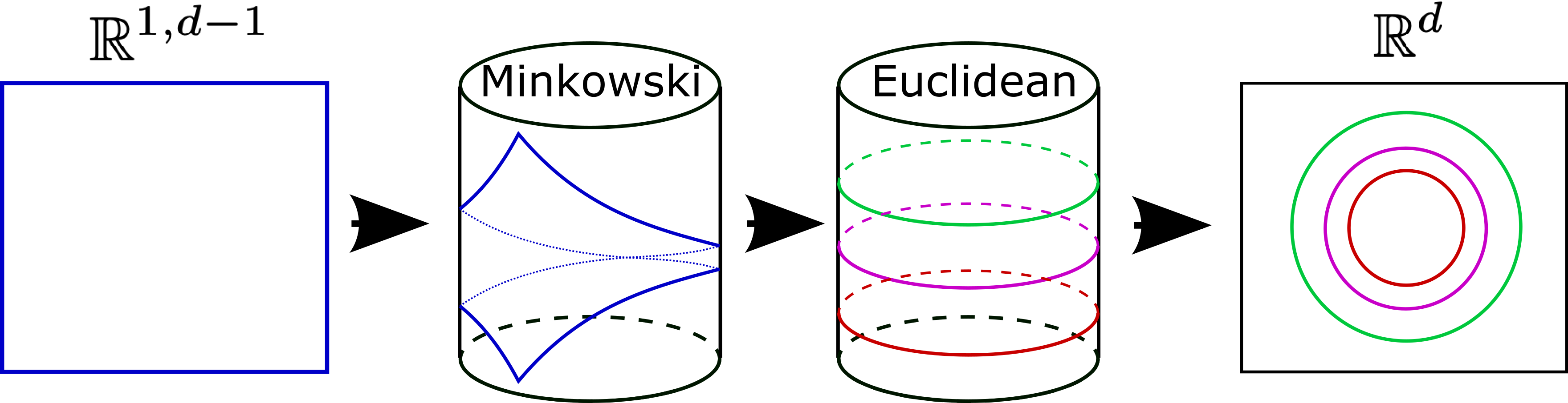
Figure 1: Minkowski plane to cylinder to Euclidean plane.

For completeness, the line element written in terms of the different coordinates reads

$$ds_{\mathbb{R}^{1,d-1}}^{2} = \frac{1}{4\cos^{2}\frac{\tau+\theta}{2}\cos^{2}\frac{\tau-\theta}{2}}\underbrace{\left(d\tau^{2}-d\theta^{2}-\sin^{2}\theta d\vec{n}^{2}\right)}_{\text{Minkowski cylinder}}$$

$$= -\frac{1}{4\cos^{2}\frac{\tau+\theta}{2}\cos^{2}\frac{\tau-\theta}{2}}\underbrace{\left(d\eta^{2}+d\theta^{2}+\sin^{2}\theta d\vec{n}^{2}\right)}_{\text{Euclidean cylinder}}$$

$$= -\frac{e^{-2\eta}}{4\cos^{2}\frac{\tau+\theta}{2}\cos^{2}\frac{\tau-\theta}{2}}ds^{2}_{\mathbb{R}^{d}}\ .$$

2.6 Radial quantization

We finish the lightning review by commenting on the radial quantization (2.52). Assuming that all the correlators are obtained from a path integral with a conformally invariant action $S_{0}[\bar{\phi}]$ it is straightforward to derive the operator-state correspondence [19, 12]. It is usually the case that a conformally invariant, unitary, theory can be put on a curved manifold in a Weyl invariant way (for examples of non-unitary theories defying this assumption see [20]). In other words, the action $S_{0}[\bar{\phi}]$ capturing the dynamics of a CFT can be generalized to $S[\bar{\phi},g_{ab}]$ that also depends on the background metric

$$S_{0}[\bar{\phi}]=S[\bar{\phi},\delta_{ab}]\to S[\bar{\phi},g_{ab}]\ ,$$ (2.54)

such that

$$S[e^{-\Delta_{W}\sigma}\bar{\phi},e^{2\sigma}g_{ab}]=S[\bar{\phi},g_{ab}]\ ,$$ (2.55)

where $\Delta_{W}$ is the Weyl weight of the field $\bar{\phi}$; if a field with scaling dimension $\Delta$ has $n_{L}$ lower and $n_{U}$ upper indices, then its Weyl weight is given by

$$\Delta_{W}=\Delta+n_{U}-n_{L}\ .$$ (2.56)

Considering a diffeomorphism corresponding to the coordinate transformation (2.52), i.e.

$$S_{0}\left[\bar{\phi}^{a\dots}_{b\dots}(z)\right]=S\left[\bar{\phi}^{{}^{\prime}a\dots}_{b\dots}(\eta,\vec{n}),e^{2\eta}(d\eta^{2}+d\Omega_{d-1}^{2})\right]\ ,$$ (2.57)

followed by a Weyl rescaling with $\sigma=\eta$, leads to

$$S\left[\bar{\phi}^{{}^{\prime}a\dots}_{b\dots}(\eta,\vec{n}),e^{2\eta}(d\eta^{2}+d\Omega_{d-1}^{2})\right]=S\left[e^{\Delta_{W}\eta}\bar{\phi}^{{}^{\prime}a\dots}_{b\dots}(\eta,\vec{n}),d\eta^{2}+d\Omega_{d-1}^{2}\right]\ .$$ (2.58)

The fact that the theory is Weyl invariant, c.f. (2.55), translates into

$$S\left[e^{\Delta_{W}\eta}\bar{\phi}^{{}^{\prime}a\dots}_{b\dots}(\eta,\vec{n}),d\eta^{2}+d\Omega_{d-1}^{2}\right]=S\left[\hat{\phi}^{a\dots}_{b\dots}(\eta,\vec{n}),d\eta^{2}+d\Omega_{d-1}^{2}\right]\ ,$$ (2.59)

implying of course the equivalence of the system on the plane and on the cylinder, i.e.

$$S_{0}\left[\bar{\phi}^{a\dots}_{b\dots}(z)\right]=S\left[\hat{\phi}^{a\dots}_{b\dots}(\eta,\vec{n}),d\eta^{2}+d\Omega_{d-1}^{2}\right]\ ,$$ (2.60)

provided we define

$$\hat{\phi}^{a\dots}_{b\dots}(\eta,\vec{n})\equiv e^{\Delta_{W}\tau}\frac{\partial z^{{}^{\prime}a}}{\partial z^{c}}\dots\frac{\partial z^{b}}{\partial z^{{}^{\prime}d}}\dots\bar{\phi}^{c\dots}_{d\dots}(z)\ ,$$ (2.61)

and $z^{\prime}$ stands for the cylinder coordinates parametrized by $\eta$ and $\vec{n}$.

It follows from (2.52) that the generator controlling translations in the cylinder’s “time” $\eta$ is identical to dilatations $\bar{D}$ on the Euclidean plane. Indeed, on the cylinder we have

$$\left[\bar{D},\hat{\phi}^{a\dots}_{b\dots}(\eta,\vec{n})\right] = e^{\Delta_{W}\eta}\frac{\partial z^{{}^{\prime}a}}{\partial z^{c}}\dots\frac{\partial z^{b}}{\partial z^{{}^{\prime}d}}\dots\left[\bar{D},\bar{\phi}^{c\dots}_{d\dots}(z)\right]$$ (2.62)

$$= -ie^{\Delta_{W}\eta}\frac{\partial z^{{}^{\prime}a}}{\partial z^{c}}\dots\frac{\partial z^{b}}{\partial z^{{}^{\prime}d}}\dots(\Delta_{W}+\partial_{\eta})\bar{\phi}^{c\dots}_{d\dots}(z)=-i\partial_{\eta}\hat{\phi}^{a\dots}_{b\dots}(\eta,\vec{n})\ ,$$

which means that the eigenstates of the Hamiltonian (controlling the evolution in real time) on the cylinder are in one-to-one with the dimensions of the fields. There are other manifolds where Hamiltonians are related to different generators of the Euclidean conformal algebra. For instance, in [21] it was shown that for $AdS_{d-1}\times\mathbb{S}^{1}$, the eigenstates of the Hamiltonian are given by the twists of the corresponding operators.

3 Non-Relativistic CFTs

In this section we present a similar construction for non-relativistic conformal field theories.

3.1 The Schrödinger algebra

The Schrödinger algebra comprises the generators of temporal and spatial translations $H$ and $P_{i}$, respectively, spatial rotations $J_{ij}$, Galilean boosts $K_{i}$, dilatations $D$ and special conformal transformations $S$. As usual, the algebra is also centrally extended by adding the particle number operator $Q$ commuting with the rest of the generators.

The standard commutation relations for the Galilei algebra

$$\left[J_{ij},J_{kl}\right] = i\left(J_{jl}\delta_{ik}+J_{ik}\delta_{jl}-J_{il}\delta_{jk}-J_{jk}\delta_{il}\right)\ ,$$

$$\left[J_{ij},P_{k}\right] = i\left(\delta_{ik}P_{j}-\delta_{jk}P_{i}\right)\ ,$$ (3.1)

$$\left[J_{ij},K_{k}\right] = i\left(\delta_{ik}K_{j}-\delta_{jk}K_{i}\right)\ ,$$

should be supplemented by the way the momenta and Hamiltonian are transformed under boosts,

$$\left[K_{i},P_{j}\right]=-i\delta_{ij}Q\ ,~{}~{}~{}\left[K_{i},H\right]=-iP_{i}\ ,\\$$ (3.2)

as well as the nonvanishing commutators involving dilation and special conformal transformations

$$\begin{array}[]{lll}\left[D,H\right]=-2iH\ ,&\left[D,P_{i}\right]=-iP_{i}\ ,\\ \left[D,K_{i}\right]=iK_{i}\ ,&\left[D,S\right]=2iS\ ,\\ \left[S,H\right]=iD\ ,&\left[S,P_{i}\right]=iK_{i}\ .\end{array}$$ (3.3)

Several comments are in order here. From (3.1), we notice that $P_{i}$ and $K_{i}$ (we are in $\mathbb{R}\times\mathbb{R}^{d}$, and the indices $i,j,\dots$ run from $1$ to $d-1$) are vectors of $SO(d-1)$. Meanwhile, inspection of (3.3) reveal that the scaling dimensions of $H$, $P_{i}$, $K_{i}$ and $S$ are $2$, $1$, $-1$ and $-2$, respectively.

3.2 Representations

The representations of the Schrödinger algebra can be build in the following way. We can choose the subalgebra spanned by $Q$, $E\equiv H-S$ and $J_{ij}$ to label any state with the eigenvalues $m$, $\varepsilon$, $j$ and $\sigma$ of $Q$, $E$ and the spins corresponding to $SO(d-1)$. For instance, in $d=4$ we have

$$E|m,\varepsilon,j,\sigma\rangle = \varepsilon|m,\varepsilon,j,\sigma\rangle\ ,$$

$$J_{ij}J_{ij}|m,\varepsilon,j,\sigma\rangle = j(j+1)|m,\varepsilon,j,\sigma\rangle\ ,$$ (3.4)

$$J_{3}|m,\varepsilon,j,\sigma\rangle = \sigma|m,\varepsilon,j,\sigma\rangle\ ,$$

$$Q|m,\varepsilon,j,\sigma\rangle = m|m,\varepsilon,j,\sigma\rangle\ .$$

It is straightforward to show that for the following linear combinations

$$F_{i}^{\pm}\equiv\frac{K_{i}\pm iP_{i}}{\sqrt{2}}\ ,~{}~{}~{}G^{\pm}=\frac{1}{2}\left[D\pm i\left(H+S\right)\right]\ ,$$ (3.5)

we have

$$\left[E,F^{\pm}_{i}\right]=F^{\pm}_{i}\ ,~{}~{}~{}\left[E,G^{\pm}\right]=2G^{\pm}\ ,$$ (3.6)

therefore these operators act as raising and lowering operators for the eigenvalues of $E$. Noting also that $(G^{-},F_{i}^{-})$ and $(G^{+},F_{i}^{+})$ form two Abelian subalgebras, we can define a lowest weight state as

$$F_{i}^{-}|m,\varepsilon,j,\sigma\rangle=G^{-}|m,\varepsilon,j,\sigma\rangle=0\ ,$$ (3.7)

and generate the whole Hilbert space by acting on it repeatedly with $(G^{+},F_{i}^{+})$. It may be advantageous to introduce spin eigenstates $F^{+}_{\alpha}$ with $\alpha=(+,0,-)$

$$F^{+}_{\pm}\equiv\frac{1}{\sqrt{2}}\left(F_{1}\pm F_{2}\right)\ ,~{}~{}~{}F_{0}^{+}\equiv F^{+}_{3}\ ,$$ (3.8)

such that

$$\left[J_{3},F^{+}_{\alpha}\right]=\alpha F^{+}_{\alpha}\ .$$ (3.9)

As a result the Hilbert space is given by a span of vectors of the form

$$|m,\varepsilon,j,\sigma;n_{+},n_{0},n_{-},k\rangle=\left(F^{+}_{+}\right)^{n_{+}}\left(F^{+}_{0}\right)^{n_{0}}\left(F^{+}_{-}\right)^{n_{-}}\left(G^{+}\right)^{k}|m,\varepsilon,j,\sigma\rangle\ ,$$ (3.10)

with $n_{+}$, $n_{0}$, $n_{-}$ and $k$ integers; the corresponding eigenvalues of $E$ and $J_{3}$ are

$$E|m,\varepsilon,j,\sigma;n_{+},n_{0},n_{-},k\rangle = (\varepsilon+n_{+}+n_{0}+n_{-}+2k)|m,\varepsilon,j,\sigma;n_{+},n_{0},n_{-},k\rangle\ ,$$

$$J_{3}|m,\varepsilon,j,\sigma;n_{+},n_{0},n_{-},k\rangle = (j+n_{+}-n_{-})|m,\varepsilon,j,\sigma;n_{+},n_{0},n_{-},k\rangle\ .$$ (3.11)

We note in passing that the four-dimensional Schrödinger algebra possesses three Casimir operators [22, 23]. One of them is obviously $Q$, while the others are quadratic and quartic in the generators of the algebra.

3.3 Action of the algebra on fields

The way the algebra acts on fields is derived in the standard way by constructing a representation induced from that of a subalgebra generated by $(Q,J,D,K,S)$—this obviously leaves the origin $(t=0,\vec{x}=0)$ invariant, therefore, we can define its action on fields there. Namely, since the generators $Q,J,D$ commute with each other, we have

$$\left[D,\phi(0)\right] = -i\Delta\phi(0)\ ,$$

$$\left[Q,\phi(0)\right] = -m\phi(0)\ ,$$ (3.12)

$$\left[J_{ij},\phi(0)\right] = i\Sigma_{ij}\phi(0)\ ,$$

where $\Delta,m$ are numbers and $\Sigma_{ij}$ is a finite-dimensional matrix corresponding to an irreducible representation of the $SO(d-1)$ spatial rotations. Assuming that a subset of fields is closed under the action of $K_{i}$ and $S$, in other words

$$\left[S,\phi(0)\right]=is\phi(0)\ ,~{}~{}~{}\left[K_{i},\phi(0)\right]=i\kappa_{i}\phi(0)\ ,$$ (3.13)

with $s$ and $\kappa_{i}$ matrices, it follows that

$$\left[\Delta,\kappa_{i}\right]=\kappa_{i}\ ,~{}~{}~{}\left[\Delta,s\right]=2s\ ,$$ (3.14)

which means that $s=\kappa=0$ and operators $S$ and $K_{i}$ are realized trivially

$$\left[S,\phi(0)\right]=0\ ,~{}~{}~{}\left[K_{i},\phi(0)\right]=0\ .$$ (3.15)

Now from

$$\left[H,\phi(t,\vec{x})\right]=-i\partial_{t}\phi(t,\vec{x})\ ,~{}~{}\left[P_{i},\phi(t,\vec{x})\right]=i\partial_{i}\phi(t,\vec{x})\ ,$$ (3.16)

equivalently,

$$\phi(t,x_{i})=e^{iHt-iP_{i}x_{i}}\phi(0)e^{-iHt+iP_{i}x_{i}}\ ,$$ (3.17)

we get 

$$\left[D,\phi(t,\vec{x})\right] = -i\left(\Delta+2t\partial_{t}+x_{i}\partial_{i}\right)\phi(t,\vec{x})\ ,$$

$$\left[Q,\phi(t,\vec{x})\right] = -m\phi(t,\vec{x})\ ,$$

$$\left[J_{ij},\phi(t,\vec{x})\right] = i\left(\Sigma_{ij}\phi(x)+x_{i}\partial_{j}-x_{j}\partial_{i}\right)\phi(x)\ ,$$ (3.18)

$$\left[S,\phi(t,\vec{x})\right] = i\left(t\Delta+t^{2}\partial_{t}+x_{i}t\partial_{i}-\frac{i}{2}mx_{i}^{2}\right)\phi(t,\vec{x})\ ,$$

$$\left[K_{i},\phi(t,\vec{x})\right] = i\left(t\partial_{i}-imx_{i}\right)\phi(t,\vec{x})\ .$$

3.4 Automorphism

To be able to construct the Hilbert space from fields the way it was done for the case of relativistic CFTs, we need to find an automorphism (up to an analytic continuation) of the Schrödinger generators

$$H,P_{i},J_{ij},D,K_{i},S~{}~{}~{}\to~{}~{}~{}\bar{H},\bar{P},\bar{J}_{ij},\bar{D},\bar{K}_{i},\bar{S},$$ (3.19)

such that the new, barred, ones have the appropriate conjugation properties.

The commutation relations involving the new generators, as well as their action on (barred) fields are of course similar to the ones we presented above. From the “barred counterpart” of (3.3), we notice that $\bar{J}$ and $\bar{Q}$ should be Hermitian while $\bar{D}$ should be anti-Hermitian

$$\bar{J}_{ij}^{\dagger}=J_{ij}\ ,~{}~{}~{}\bar{Q}^{\dagger}=\bar{Q}\ ,~{}~{}~{}\bar{D}^{\dagger}=-\bar{D}\ .$$ (3.20)

As $Q$ is just the central charge we can immediately fix $\bar{Q}=Q$. To preserve the structure of the commutation relations (3.2) and (3.3), one should impose specific conjugation properties for the rest of the operators. For instance,

$$\left[\bar{D},\bar{H}^{\dagger}\right]=-\left[\bar{D}^{\dagger},\bar{H}^{\dagger}\right]=\left[\bar{D},\bar{H}\right]^{\dagger}=(-2i\bar{H})^{\dagger}=2i\bar{H}^{\dagger}\ ,$$ (3.21)

which can be satisfied, provided we identify

$$\bar{H}^{\dagger}=\bar{S}\ .$$ (3.22)

This automatically implies

$$\left[\bar{S},\bar{H}\right]=-\left[\bar{H},\bar{S}\right]=-\left[\bar{S}^{\dagger},\bar{H}^{\dagger}\right]=\left[\bar{S},\bar{H}\right]^{\dagger}=(i\bar{D})^{\dagger}=i\bar{D}\ ,$$ (3.23)

which is essentially the same as for the relativistic conformal group (2.25). The difference comes for $P_{i}$ and $K_{i}$. Indeed, we have

$$\left[\bar{D},\bar{P}_{i}^{\dagger}\right]=-\left[\bar{D}^{\dagger},\bar{P}_{i}^{\dagger}\right]=\left[\bar{D},\bar{P}_{i}\right]^{\dagger}=(-i\bar{P}_{i})^{\dagger}=i\bar{P}_{i}^{\dagger}\ ,$$ (3.24)

which is clearly satisfied for

$$\bar{P}_{i}^{\dagger}=\alpha_{1}\bar{K}_{i}\ ,$$ (3.25)

with $\alpha_{1}$ a complex number. Similarly,

$$\left[\bar{D},\bar{K}_{i}^{\dagger}\right]=-\left[\bar{D}^{\dagger},\bar{K}_{i}^{\dagger}\right]=\left[\bar{D},\bar{K}_{i}\right]^{\dagger}=(i\bar{K}_{i})^{\dagger}=-i\bar{K}_{i}^{\dagger}\ ,$$ (3.26)

for which

$$\bar{K}_{i}^{\dagger}=\alpha_{2}\bar{P}_{i}\ ,$$ (3.27)

where $\alpha_{2}$ is also a complex number. Note that for operators with $\bar{Q}\neq 0$, the constants $\alpha_{1}$ and $\alpha_{2}$ are constrained as 

$$\alpha_{1}\alpha_{2}=-1\ ,$$ (3.29)

since

$$[\bar{K}_{i},\bar{P}_{j}]^{\dagger}=\alpha_{1}\alpha_{2}\left[\bar{K}_{j},\bar{P}_{i}\right]=i\delta_{ij}\bar{Q}\ ,$$ (3.30)

and

$$[\bar{K}_{i},\bar{P}_{j}]=-i\delta_{ij}\bar{Q}\ .$$ (3.31)

Taking also into account that

$$\bar{P}_{i}=(\bar{P}_{i}^{\dagger})^{\dagger}\ ,~{}~{}~{}\bar{K}_{i}=(\bar{K}_{i}^{\dagger})^{\dagger}\ ,$$ (3.32)

leads to

$$\alpha^{*}_{1,2}=-\alpha_{1,2}\ ,$$ (3.33)

so we choose $\alpha_{1}=\alpha_{2}=i$, i.e.

$$\bar{P}_{i}^{\dagger}=i\bar{K}_{i}\ ,~{}~{}~{}\bar{K}_{i}^{\dagger}=i\bar{P}_{i}\ .$$ (3.34)

Now we move to finding the needed automorphism. Noting that the subalgebra generated by $H$, $S$ and $D$ is identical (modulo the sign of $S$) to that generated by $P_{0}$, $K_{0}$ and $D$, we can guess immediately the appropriate transformation. Namely (compare with (2.21)) we consider an automorphism of the Schrödinger algebra generated by a linear combination of $H$ and $S$

$$\exp\left[\frac{\pi}{4}(H+S)\right]\ .$$ (3.35)

Using the results of Appendix E we obtain ($\bar{Q}=Q$ and $\bar{J}_{ij}=J_{ij}$)

$$\bar{P}_{i} = \frac{1}{\sqrt{2}}\left(P_{i}-iK_{i}\right)\ ,$$

$$\bar{K}_{i} = \frac{1}{\sqrt{2}}\left(-iP_{i}+K_{i}\right)\ ,$$

$$\bar{S} = \frac{1}{2}\left(H+S+iD\right)\ ,$$ (3.36)

$$\bar{H} = \frac{1}{2}\left(H+S-iD\right)\ ,$$

$$\bar{D} = -i\left(H-S\right)\ .$$

Comparing with (3.5) we see that, as we wanted, the newly constructed generators are in one to one correspondence with those used in Section 3.2 to construct the representations of the Schrödinger algebra

$$\bar{P}_{i}=-iF_{i}^{+}\ ,~{}~{}~{}\bar{K}_{i}=F_{i}^{-}\ ,~{}~{}~{}\bar{S}=iG^{-}\ ,~{}~{}~{}\bar{H}=-iG^{+}\ ,~{}~{}~{}\bar{D}=-iE\ .$$ (3.37)

Using expressions completely analogous to the ones presented in Eqs. (2.28)-(2.31) for the non-relativistic case finalizes the construction of the Hilbert space in terms of local operators.

3.5 Coordinate transformations

We will now identify the coordinate transformation that actually corresponds to the automorphism of the Schrödinger algebra discussed above. Let us denote the new coordinates by $(s,\vec{z})$. As in Sec. (2.5.1), we shall use the explicit representation of the generators in the two coordinate systems in terms of differential operators, i.e.

$$P_{i}=-i\partial^{x}_{i},~{}H=i\partial_{t}\ , D=i(2t\partial_{t}+x_{i}\partial^{x}_{i})\ ,~{}~{}~{}K_{i}=-it\partial^{x}_{i}\ ,$$

$$S=-i(t^{2}\partial_{t}+x_{i}t\partial^{x}_{i})\ , J_{ij}=-i(x_{i}\partial^{x}_{j}-x_{j}\partial^{x}_{i})\ ,$$ (3.38)

and

$$\bar{P}_{i}=-i\partial^{z}_{i}\ ,~{}~{}~{}\bar{H}=i\partial_{s}\ , \bar{D}=i(2s\partial_{s}+z_{i}\partial^{z}_{i})\ ,~{}~{}~{}\bar{K}_{i}=-is\partial^{z}_{i}\ ,$$

$$\bar{S}=-i(s^{2}\partial_{t}+z_{i}s\partial^{z}_{i})\ , \bar{J}_{ij}=-i(z_{i}\partial^{z}_{j}-z_{j}\partial^{z}_{i})\ .$$ (3.39)

From the above expressions we obtain

$$is=\frac{1+it}{1-it}\ ,~{}~{}~{}z_{i}=\sqrt{2}\frac{x_{i}}{1-it}\ .$$ (3.40)

The corresponding transformation of a scalar primary field can be deduced from (F.18) (see Appendix F for the explicit derivation) and reads 

$$\phi(t,\vec{x})=\frac{2^{\Delta/2}}{(1-it)^{\Delta}}\exp\left({\frac{m\vec{x}^{2}}{2(1-it)}}\right)\bar{\phi}\left(-i\frac{1+it}{1-it},\frac{\vec{x}\sqrt{2}}{1-it}\right)\ .$$ (3.41)

Given the relation between fields in different frames we can find how $\bar{\phi}$ transforms under Hermitian conjugation 

$$\bar{\phi}^{\dagger}(s,\vec{z})=(-is)^{-\Delta}\exp\left(i{\frac{m\vec{z}^{2}}{2s}\frac{1+is}{1-is}}\right)\bar{\phi}^{*}\left(\frac{1}{s},\frac{i\vec{z}}{s}\right)\ .$$ (3.44)

One can check that the so-defined Hermitian conjugation preserves the action of the Schrödinger algebra on fields (3.3) and at the same time is consistent with the conjugation properties (3.22) and (3.34).

3.6 NRCFT and geometric data

It is well-known [1, 24, 3, 25, 26] that coupling a non-relativistic system to a non-trivial gravitational background (geometry) can be achieved by introducing appropriate gauge fields (analogues of metric and connection in general relativity, see Appendix G). Namely, the needed geometric data are the temporal and spatial parts of a vielbein—$n_{\mu}$, $e^{i}_{\mu}$, respectively—and a gauge field $A_{\mu}$ corresponding to the $U(1)$ transformations generated by the particle number operator.

The non-relativistic conformal transformations can be defined similarly to the relativistic ones. Starting form a trivial (flat) background, corresponding to

$$n_{\mu}(t,\vec{x})=\delta_{\mu}^{0}\ ,~{}~{}~{}e_{\mu}^{i}(t,\vec{x})=\delta_{\mu}^{i}\ ,~{}~{}~{}A_{\mu}(t,\vec{x})=0\ ,$$ (3.45)

we call conformal those coordinate transformations that lead to a change of the geometric data by a conformal factor

$$n^{\prime}_{\mu}(t^{\prime},\vec{x}^{\prime}) \simeq f^{2}(t,\vec{x})\delta_{\mu}^{0}\ ,$$ (3.46)

$$e^{{}^{\prime}i}_{\mu}(t^{\prime},\vec{x}^{\prime}) \simeq f(t,\vec{x})\delta_{\mu}^{i}\ ,$$ (3.47)

$$A^{\prime}_{\mu}(t^{\prime},\vec{x}^{\prime}) \simeq 0\ .$$ (3.48)

Here “$\simeq$” is understood as an equality modulo possible gauge transformations listed in Table G.11. Introducing the infinitesimal change of coordinates

$$t^{\prime}=t+\xi_{t}\ ,~{}~{}x_{i}^{\prime}=x_{i}+\xi_{i}\ ,$$ (3.49)

and denoting $f=1+\psi$, we see from (3.46) that $\xi_{t}=\xi_{t}(t)$ and

$$\psi(t)=-\frac{1}{2}\partial_{t}\xi_{t}\ .$$ (3.50)

The temporal ($\mu=t$) component of (3.47) can be satisfied by using a boost transformation with parameter $v_{i}=-\partial_{t}\xi_{i}$. For the spatial ($\mu=j$) components of (3.47) we get

$$(1+\psi)\delta_{ij}=\delta_{ij}-\partial_{j}\xi_{i}+r_{ij}\ ,$$ (3.51)

where $r_{ij}$ is an antisymmetric matrix corresponding to gauge rotations of the vielbein (see Table G.11). Symmetrizing the above and using (3.50) we obtain

$$\partial_{i}\xi_{j}+\partial_{j}\xi_{i}=\delta_{ij}\partial_{t}\xi_{t}\ ,$$ (3.52)

whose solution is clearly at most linear in $x_{i}$

$$\xi_{i}=\frac{1}{2}\partial_{t}\xi_{t}x_{i}+b_{ij}(t)x_{j}+c_{i}(t)\ ,~{}~{}~{}b_{ij}(t)=-b_{ji}(t)\ .$$ (3.53)

Bearing in mind that the $U(1)$ gauge field produced by the boost transformation with parameter $v_{i}=-\partial_{t}\xi_{i}$

$$A_{t}=0\ ,~{}~{}~{}A_{i}=-\partial_{t}\xi_{i}=-\left(\frac{1}{2}\partial^{2}_{t}\xi_{t}x_{i}+\partial_{t}b_{ij}(t)x_{j}+\partial_{t}c_{i}(t)\right)\ ,$$ (3.54)

can be eliminated by a $U(1)$ transformation only if $\partial^{2}_{t}\xi_{t}=\mathrm{const}$, $\partial_{t}b_{ij}(t)=0$, and $\partial_{t}c_{i}(t)=\mathrm{const}$, we find the following expression for the infinitesimal transformations

$$\xi_{t}=c_{t}+2\lambda t+\mu t^{2}\ ,~{}~{}\xi_{i}=c_{i}+d_{i}t+b_{ij}x_{j}+\lambda x_{i}+\mu tx_{i}\ .$$ (3.55)

The above correspond to time and space translations, rotations, boosts, dilations and special conformal transformations.

3.7 The analogue of radial quantization

In order to have complete analogy with the relativistic case, we will show here what happens if one considers dilatations generated by $\bar{D}$ as the corresponding Hamiltonian. It was shown in [26] that with minor assumptions an NRCFT can be coupled to a non-trivial background (geometric data) in a Weyl invariant manner, i.e. one constructs the curved-spacetime counterpart of a Schrödinger-symmetric action

$$S_{0}[\phi]=S[\phi,0,\delta_{\mu}^{0},\delta_{\mu}^{i}]\to S[\phi,A_{\mu},n_{\mu},e_{\mu}^{i}]\ ,$$ (3.56)

such that it is manifestly invariant under Weyl rescalings

$$S[\phi\Omega^{-\Delta},A_{\mu},n_{\mu}\Omega^{2\Delta},e_{\mu}^{i}\Omega^{\Delta}]=S[\phi,A_{\mu},n_{\mu},e_{\mu}^{i}]\ ,$$ (3.57)

with $\Omega$ the conformal factor.

For the case at hand we start from flat space and consider the following change of coordinates 

$$is=e^{2i\tau}\ ,~{}~{}~{}z_{i}=\sqrt{2}y_{i}e^{i\tau}\ ,$$ (3.59)

which amounts to replacing the temporal and spatial Kronecker symbols by the corresponding vielbeins (the relevant transformation properties for the geometrical quantities can be derived using the Table G.11)

$$n_{\mu}=2e^{2i\tau}(1,\vec{0}),~{}~{}e^{i}_{\mu}=\sqrt{2}e^{i\tau}\left(i\vec{y},\mathbb{1}\right)\ .$$ (3.60)

We find that the action becomes

$$S\left[\bar{\phi}(s,\vec{z}),0,\delta_{\mu}^{s},\delta_{\mu}^{i}\right]=S\left[\bar{\phi}^{\prime}(\tau,\vec{y}),0,n_{\mu},e_{\mu}^{i}\right]\ ,$$ (3.61)

with $\bar{\phi}^{\prime}(\tau,\vec{y})=\bar{\phi}(s,\vec{z})$. Then, we perform a Weyl rescaling with $\Omega=\sqrt{2}e^{i\tau}$, yielding

$$S\left[\bar{\phi}(s,\vec{z}),0,n_{\mu},e_{\mu}^{i}\right]=S\left[2^{\Delta/2}e^{i\Delta\tau}\bar{\phi}^{\prime}(\tau,\vec{y}),0,\delta_{\mu}^{\tau},\left(i\vec{y},\mathbb{1}\right)\right]\ .$$ (3.62)

Next, in order to bring the vielbein to its original form, we consider a boost with parameter $v_{i}=-iy_{i}$, such that

$$S\left[2^{\Delta/2}e^{i\Delta\tau}\bar{\phi}^{\prime}(\tau,\vec{y}),0,\delta_{\mu}^{\tau},\left(i\vec{y},\mathbb{1}\right)\right]=S\left[2^{\Delta/2}e^{i\Delta\tau}\bar{\phi}^{\prime}(\tau,\vec{y}),A_{\mu},\delta_{\mu}^{\tau},\delta_{\mu}^{i}\right]\ ,$$ (3.63)

which results also in the generation of the following $U(1)$ gauge field

$$A_{s}=\frac{\vec{y}^{2}}{2}\ ,~{}~{}~{}A_{i}=-iy_{i}\ .$$ (3.64)

Lastly, performing a $U(1)$ gauge transformation with parameter $\alpha=i\frac{\vec{y}^{2}}{2}$ we can eliminate the spatial part $A_{i}$, to obtain

$$S_{0}[\bar{\phi}(s,\vec{z})]=S\left[\hat{\phi}(\tau,\vec{y})\ ,\hat{A}_{\mu}(\tau,\vec{y}),\delta_{\mu}^{\tau},\delta_{\mu}^{i}\right]\ ,$$ (3.65)

with

$$\hat{\phi}(\tau,\vec{y})=2^{\frac{\Delta}{2}}e^{i\Delta\tau}e^{\frac{m\vec{y}^{2}}{2}}\bar{\phi}(s,\vec{z})\ ,~{}~{}~{}\hat{A}_{\tau}=\frac{\vec{y}^{2}}{2}\ .$$ (3.66)

Note that the form of the transformed field $\hat{\phi}$ is consistent with (F.18). Equation (3.65) is the analogue of putting a CFT on the cylinder. It tells us that the systems with and without harmonic potential are equivalent.

A straightforward computation – completely analogous to the one we explicitly carried out in Sec. 2.6, see Eq. (2.62) – reveals that in this frame, dilatation $\bar{D}$ acts on operators $\hat{\phi}$ as time translations, i.d. it plays the role of a Hamiltonian

$$\left[i\bar{D},\hat{\phi}(\tau,\vec{y})\right] = 2^{\frac{\Delta}{2}}e^{i\Delta\tau}e^{\frac{m\vec{y}^{2}}{2}}\left[i\bar{D},\bar{\phi}(s,\vec{z})\right]$$ (3.67)

$$= \,2^{\frac{\Delta}{2}}e^{i\Delta\tau}e^{\frac{m\vec{y}^{2}}{2}}\left(\Delta+2s\partial_{s}+z_{i}\partial_{i}^{z}\right)\bar{\phi}(s,\vec{z})=-i\partial_{\tau}\hat{\phi}(\tau,\vec{y})\ .$$

Clearly, this means that the spectrum of the Hamiltonian in the harmonic frame is in one to one correspondence with the spectrum of scaling dimensions of operators.

4 Conclusions

A powerful tool when it comes to studying relativistic and nonrelativistic conformal field theories is the operator-state map, in particular, the correspondence between the scaling dimensions of operators and the “energy spectrum” of the associated states.

In this paper we introduced an algebraic in nature perspective on the aforementioned correspondence. The crucial observation is that the Hilbert space associated with the conformal algebra may be constructed by Euclidean fields. This implies that the operator-state map is obtained by establishing the appropriate relation (automorphism) between the generators of the Minkowski-space conformal algebra and their Euclidean-space counterparts together with the OPE.

Using the derivation in CFT as a guide, we extended the construction to NRCFTs, for which we recover the well-known correspondence between the operators in the theory and states of the system supplemented by an oscillator potential.

Appendix A An alternative automorphism in $d=3$ dimensions

In this appendix we discuss an alternative to the automorphism discussed in the main text. For clarity, we confine ourselves to $d=3$. As before, we denote with $M_{AB}$ the generators of $SO(2,3)$ that satisfy the commutation relations (2.6), i.e.

$$\left[M_{AB},M_{CD}\right]=i\left(M_{AD}\eta_{BC}+M_{BC}\eta_{AD}-M_{BD}\eta_{AC}-M_{AC}\eta_{BD}\right)\ ,$$ (A.1)

with the five-dimensional metric

$$\eta_{AB}=\left(+,-,-,-,+\right)\ .$$ (A.2)

The automorphism we are after corresponds to introducing the rotated, “barred generators” $\bar{M}_{AB}$, which are related to the original ones via successive $\pi/2$ rotations in the $(0,3)$-, $(4,1)$-, and $(0,2)$- planes:

$$\bar{M}_{AB}=e^{-i\frac{\pi}{2}M_{02}}e^{i\frac{\pi}{2}M_{41}}e^{i\frac{\pi}{2}M_{03}}M_{AB}e^{-i\frac{\pi}{2}M_{03}}e^{-i\frac{\pi}{2}M_{41}}e^{i\frac{\pi}{2}M_{02}}\ .$$ (A.3)

Explicitly, the above yields

$$\bar{M}_{01}=M_{43}\ ,~{}~{}~{}\bar{M}_{02}=M_{30}\ ,~{}~{}~{}\bar{M}_{12}=M_{40}\ ,$$

$$\bar{M}_{30}=-iM_{32}\ ,~{}~{}~{}\bar{M}_{31}=-iM_{42}\ ,~{}~{}~{}\bar{M}_{32}=iM_{02}\ ,$$

$$\bar{M}_{40}=M_{31}\ ,~{}~{}~{}\bar{M}_{41}=M_{41}\ ,~{}~{}~{}\bar{M}_{42}=-M_{01}\ ,~{}~{}~{}\bar{M}_{43}=iM_{12}\ .$$ (A.4)

which in turn results into the following map

$$\bar{D}=iJ_{12}\ ,~{}~{}~{}\bar{J}_{01}=D\ ,~{}~{}~{}\bar{J}_{02}=\frac{1}{2}\left(P_{0}-K_{0}\right)\ ,~{}~{}~{}\bar{J}_{12}=\frac{1}{2}\left(P_{0}+K_{0}\right)\ ,$$

$$\bar{P}_{0}=\frac{1}{2}\left[P_{1}-K_{1}-i\left(P_{2}-K_{2}\right)\right]\ ,~{}~{}~{}\bar{K}_{0}=\frac{1}{2}\left[P_{1}-K_{1}+i\left(P_{2}-K_{2}\right)\right]\ ,$$

$$\bar{P}_{1}=\frac{1}{2}\left[P_{1}+K_{1}-i\left(P_{2}+K_{2}\right)\right]\ ,~{}~{}~{}\bar{K}_{1}=\frac{1}{2}\left[P_{1}+K_{1}+i\left(P_{2}+K_{2}\right)\right]\ ,$$

$$\bar{P}_{2}=-\left(J_{01}-iJ_{02}\right)\ ,~{}~{}~{}\bar{K}_{2}=-\left(J_{01}+iJ_{02}\right)\ .$$ (A.5)

The first thing to note here is that the generators $\bar{J}_{\mu\nu}$ are Hermitian. Therefore, if we want to realize the Hilbert space on the space of fields, or in other words

$$|\Phi\rangle=\Phi(0)|0\rangle\ ,$$ (A.6)

the equation

$$\left[\bar{J}_{\mu\nu},\Phi(0)\right]=i\Sigma_{\mu\nu}\Phi(0),$$ (A.7)

necessitates that $\Phi(0)$ be an infinite-component field [27, 28, 29, 30]. From Eqs. (2.2) we find that its spin is $h$, therefore not bound to be half-integer, and at the same time

$$\left[\bar{D},\Phi(0)\right]=im\Phi(0)\ .$$ (A.8)

The corresponding expressions for the lowering generators (2.8) are given by

$$M_{1}^{-}=\frac{1}{2}\left[\bar{P}_{1}-i\bar{P}_{2}+\bar{K}_{1}-i\bar{K}_{2}\right]\ ,$$

$$M_{2}^{-}=\frac{i}{2}\left[\bar{P}_{1}-i\bar{P}_{2}-\left(\bar{K}_{1}-i\bar{K}_{2}\right)\right]\ ,$$

$$M_{3}^{-}=\bar{J}_{01}-i\bar{J}_{02}\ .$$ (A.9)

Clearly, in this frame the states in the Hilbert space are not given by primary fields at zero. Instead, the fields should satisfy the following constraints

$$\left(\partial_{1}-i\partial_{2}\right)\Phi(0)=0\ ,~{}~{}~{}\left[\bar{K}_{1}-i\bar{K}_{2},\Phi(0)\right]=0\ ,~{}~{}~{}(\Sigma_{01}-i\Sigma_{02})\Phi(0)=0\ .$$ (A.10)

Appendix B Conformal OPE

Here we discuss the constraints conformal invariance imposes on the OPE. We start from the general expression

$$\bar{\phi}_{2}(z_{2})\bar{\phi}_{1}(z_{1})=\sum_{\mathcal{O}}c_{12\mathcal{O}}(z_{2},z_{1})\bar{\mathcal{O}}(z_{1})\ ,$$ (B.1)

without assuming that the sum runs only over primary fields.

Let us start with translations. Acting with $\bar{P}_{a}$ on both sides of the above, we immediately find

$$\partial_{a}^{z_{1}}c_{12\mathcal{O}}(z_{2},z_{1})+\partial_{a}^{z_{2}}c_{12\mathcal{O}}(z_{2},z_{1})=0\ ,$$ (B.2)

meaning that

$$c_{12\mathcal{O}}(z_{2},z_{1})=c_{12\mathcal{O}}(z_{2}-z_{1})\ .$$ (B.3)

For the Lorentz transformations—generated by $\bar{J}_{ab}$—the expansion (B.1) gives 

$$\Sigma^{1}_{ab,\{c\}\{p\}}c_{12\mathcal{O}}^{\{p\}\{d\}\{f\}}(z)+\Sigma^{2}_{ab,\{d\}\{p\}}c_{12\mathcal{O}}^{\{c\}\{p\}\{f\}}(z)$$

$$\hskip 71.13188pt+\Sigma^{\mathcal{O}}_{ab,\{f\}\{p\}}c_{12\mathcal{O}}^{\{c\}\{d\}\{p\}}(z)+(z_{a}\partial_{b}-z_{b}\partial_{a})c_{12\mathcal{O}}^{\{c\}\{d\}\{f\}}(z)=0\ ,$$ (B.4)

where $\{\cdot\}$ stands for (possibly multiple) indices corresponding to the $SO(d)$ representation of the operators. This relation implies that if $\bar{\phi}_{1}$, $\bar{\phi}_{2}$ and $\bar{\mathcal{O}}$ are traceless symmetric tensors of ranks $l$, $m$ and $n$, respectively, we get for the function $c_{12\mathcal{O}}$

$$c_{12\mathcal{O}}^{\{c\}\{d\}\{f\}}(z) = z_{c_{1}}\dots z_{c_{l}}z_{d_{1}}\dots z_{d_{m}}z_{f_{1}}\dots z_{f_{n}}A_{l+m+n}(z^{2})$$ (B.5)

$$+\delta_{c_{1}d_{1}}z_{c_{2}}\dots z_{c_{l}}z_{d_{2}}\dots z_{d_{m}}z_{f_{1}}\dots z_{f_{n}}A^{12}_{l+m+n-2}(z^{2})$$

$$+\delta_{c_{1}f_{1}}z_{c_{2}}\dots z_{c_{l}}z_{d_{1}}\dots z_{d_{m}}z_{f_{2}}\dots z_{f_{n}}A^{13}_{l+m+n-2}(z^{2})$$

$$+\delta_{d_{1}f_{1}}z_{c_{1}}\dots z_{c_{l}}z_{d_{2}}\dots z_{d_{m}}z_{f_{2}}\dots z_{f_{n}}A^{23}_{l+m+n-2}(z^{2})+\dots\ ,$$

where $\dots$ stand for all other terms that can be obtained from contracting indices belonging to the different sets $\{c\}$, $\{d\}$ and $\{f\}$.

Similarly, acting with $\bar{D}$ on the OPE, we obtain

$$\left(\Delta_{1}+\Delta_{2}-\Delta\right)c_{12\mathcal{O}}(z)+z^{a}\partial_{a}c_{12\mathcal{O}}(z)=0\ .$$ (B.6)

In other words, dilatations fix the coefficient functions to be of the following form

$$c_{12\mathcal{O}}(z)=|z|^{\Delta-\Delta_{1}-\Delta_{2}}F\left(n_{a}\right),~{}~{}~{}n_{a}=\frac{z_{a}}{|z|}\ ,~{}~{}~{}|z|=\sqrt{z_{a}z^{a}}\ .$$ (B.7)

Using all the constraints we got so far, we can write down the OPE of two primary fields with spins $l_{1}$ and $l_{2}$ (i.e. two traceless symmetric tensors of ranks $l_{1}$ and $l_{2}$, respectively); this reads

$$\bar{\phi}^{\{a\}_{l_{2}}}_{2}(z)\bar{\phi}^{\{b\}_{l_{1}}}_{1}(0) = \sum_{\mathcal{O}}|z|^{\Delta_{\mathcal{O}}-\Delta_{1}-\Delta_{2}}\left[\lambda^{(l_{1}+l_{2}+l_{\mathcal{O}})}_{\mathcal{O}}n^{a_{1}}\dots n^{a_{l_{2}}}n^{b_{1}}\dots n^{b_{l_{1}}}n^{c_{1}}\dots n^{c_{l_{\mathcal{O}}}}\right.$$

$$+ \left.\lambda^{(l_{1}+l_{2}+l_{\mathcal{O}}-2)}_{\mathcal{O}}\delta^{a_{1}b_{1}}n^{a_{2}}\dots n^{a_{l_{1}}}n^{b_{2}}\dots n^{b_{l_{2}}}n^{c_{1}}\dots n^{c_{l_{\mathcal{O}}}}+\dots\right]\mathcal{O}^{\{c\}_{l_{\mathcal{O}}}}(0)\ ,$$

where the sum still runs over all possible operators.

What remains to be understood is what new information on the OPE we extract once we require that it be consistent with special conformal transformations. It turns out that the contributions of descendants are intrinsically linked to those of the corresponding primaries. Schematically, for every $\lambda$ (their number can be found in [31]), we get

$$\bar{\phi}^{\{a\}_{l_{2}}}_{2}(z)\bar{\phi}^{\{b\}_{l_{1}}}_{1}(0)=\sum_{\bar{\phi}}|z|^{\Delta_{\mathcal{O}}-\Delta_{1}-\Delta_{2}}\times$$

$$\hskip 14.22636pt\times\left\{\lambda^{(l_{1}+l_{2}+l)}_{12\bar{\phi}}n^{a_{1}}\dots n^{b_{1}}\dots n^{c_{1}}\dots\left[\phi^{c_{1}\dots c_{l}}(0)+a^{(l_{1}+l_{2}+l)}z_{c}\partial_{c}\phi^{c_{1}\dots c_{l}}(0)+\dots\right]+\dots\right\}\ .$$

Note that owing to conformal symmetry, all the coefficients appearing in front of the descendants are fixed. For the OPE of scalar operators those can be found in [32]. On the other hand, for operators with non-zero spin we get

$$a^{(l_{1}+l_{2}+l)}=\frac{\Delta_{21}+\Delta+l_{21}+l}{2(\Delta+l)}\ ,~{}~{}~{}\Delta_{21}=\Delta_{2}-\Delta_{1}\ ,~{}~{}~{}l_{21}=l_{2}-l_{1}\ .$$ (B.8)

Appendix C Hermitian conjugation & compatibility with the conformal algebra

It is instructive to explicitly show that the way we defined Hermitian conjugation, see Eqs. (2.32)-(2.34), does not spoil the action of the conformal algebra on fields. In what follows we work with vectors, for which

$$\bar{\phi}^{\dagger}_{a}(z)=z^{-2\Delta}I_{a}^{b}(z)\bar{\phi}_{b}(Iz)\ .$$ (C.1)

Before moving on, let us present some useful formulas. We note that

$$\partial_{a}^{Iz}=z^{2}I_{a}^{b}(z)\partial_{b}^{z}\ ,$$ (C.2)

and

$$\partial_{c}I_{ab}(z)=\frac{2}{z^{2}}\left(\frac{2z_{a}z_{b}z_{c}}{z^{2}}-\delta_{ac}z_{b}-\delta_{bc}z_{a}\right)\ ,$$ (C.3)

which imply

$$I_{a}^{d}(z)\partial_{c}I_{bd}(z)=\frac{2}{z^{2}}\left(z_{a}\delta_{bc}-z_{b}\delta_{ac}\right)\ ,$$ (C.4)

and

$$z^{-2\Delta}I_{a}^{b}(z)\partial_{c}^{z}\bar{\phi}_{b}(Iz)=\partial_{c}\bar{\phi}_{a}^{\dagger}(z)+2\Delta\frac{z_{c}}{z^{2}}\bar{\phi}^{\dagger}_{a}(z)+\frac{2}{z^{2}}\left(z_{a}\delta_{bc}-z_{b}\delta_{ac}\right)\bar{\phi}^{\dagger}_{b}(z)\ .$$ (C.5)

Using the above, we now turn to the action of the generators on the vector field; the computations are straightforward but a bit long.

We start from translations, for which

$$\left[\bar{P}_{a},\bar{\phi}_{b}(z)\right]^{\dagger} \overset{(\ref{eq:HermCFT})}{=}-\left[\bar{K}_{a},\bar{\phi}^{\dagger}_{b}(z)\right]$$ (C.6)

$$\overset{(\ref{eq:GeneratorsFieldsEuclideanAction})}{\underset{(\ref{eq:app_field})}{=}}-i\left[\left(2\frac{z_{a}z^{c}}{z^{2}}-\delta^{c}_{a}\right)\frac{z^{-2\Delta}}{z^{2}}I_{b}^{d}(z)\partial_{c}^{Iz}\bar{\phi}_{d}(Iz)+\frac{2}{z^{2}}\left(z_{a}\Delta_{\phi}\delta^{d}_{b}+z^{c}\Sigma_{ab,c}^{~{}~{}~{}d}\right)\bar{\phi}^{\dagger}_{d}(z)\right]$$

$$\overset{(\ref{eq:derivativezIz})}{=}-i\left[\left(2\frac{z_{a}z^{c}}{z^{2}}-\delta^{c}_{a}\right)I_{c}^{e}(z)z^{-2\Delta}I_{b}^{d}(z)\partial_{e}^{z}\bar{\phi}_{d}(Iz)+\frac{2}{z^{2}}\left(z_{a}\Delta_{\phi}\delta^{d}_{b}+z^{c}\Sigma_{ab,c}^{~{}~{}~{}d}\right)\bar{\phi}^{\dagger}_{d}(z)\right]$$

$$\overset{(\ref{eq:derivativephidagger})}{=}i\partial_{a}\bar{\phi}^{\dagger}_{b}(z)\ .$$

Moving to Lorentz transformations, it is easy to see that

$$\left[\bar{J}_{ab},\bar{\phi}_{c}(z)\right]^{\dagger} \overset{(\ref{eq:HermCFT})}{=}-\left[\bar{J}_{ab},\bar{\phi}^{\dagger}_{c}(z)\right]$$ (C.7)

$$\overset{(\ref{eq:GeneratorsFieldsEuclideanAction})}{\underset{(\ref{eq:app_field})}{=}}-i\Sigma_{ab,c}^{~{}~{}~{}d}\bar{\phi}^{\dagger}_{d}(z)-i\frac{z^{-2\Delta}}{z^{2}}\left(z_{a}I_{b}^{d}(z)-z_{b}I_{a}^{d}(z)\right)\partial_{d}^{Iz}\bar{\phi}_{c}(Iz)$$

$$\overset{(\ref{eq:derivativezIz})}{=}-i\Sigma_{ab,c}^{~{}~{}~{}d}\bar{\phi}^{\dagger}_{d}(z)-iz^{-2\Delta}\left(z_{a}I_{b}^{d}(z)-z_{b}I_{a}^{d}(z)\right)I_{c}^{e}(z)\partial_{e}^{z}\bar{\phi}_{c}(Iz)$$

$$\overset{(\ref{eq:derivativephidagger})}{=}-i\left(\Sigma_{ab,c}^{~{}~{}~{}d}+\left(z_{a}\partial_{b}-z_{b}\partial_{a}\right)\delta^{d}_{c}\right)\bar{\phi}^{\dagger}_{d}(z)\ ,$$

where the spin matrices $\Sigma_{ab,cd}$ for vectors are defined in (2.15).

For dilatations, a completely analogous computation shows that

$$\left[\bar{D},\bar{\phi}_{b}(z)\right]^{\dagger} \overset{(\ref{eq:HermCFT})}{=}\left[\bar{D},\bar{\phi}^{\dagger}_{b}(z)\right]$$ (C.8)

$$\overset{(\ref{eq:GeneratorsFieldsEuclideanAction})}{\underset{(\ref{eq:app_field})}{=}}-i\Delta\bar{\phi}^{\dagger}_{b}(z)-i\frac{z^{a}}{z^{2}}z^{-2\Delta}I^{c}_{b}(z)\partial_{a}^{Iz}\bar{\phi}_{c}(Iz)$$

$$\overset{(\ref{eq:derivativezIz})}{=}-i\Delta\bar{\phi}^{\dagger}_{b}(z)-iz^{a}z^{-2\Delta}I^{c}_{b}(z)I^{d}_{a}(z)\partial_{d}^{z}\bar{\phi}^{\dagger}_{c}(z)$$

$$\overset{(\ref{eq:derivativephidagger})}{=}i\left(\Delta+z^{a}\partial_{a}\right)\bar{\phi}^{\dagger}_{b}(z)\ .$$

Finally, the action of special conformal transformations reads

$$\left[K_{a},\bar{\phi}_{b}(z)\right]^{\dagger} \overset{(\ref{eq:HermCFT})}{=}-\left[P_{a},\bar{\phi}^{\dagger}_{b}(z)\right]$$ (C.9)

$$\overset{(\ref{eq:GeneratorsFieldsEuclideanAction})}{\underset{(\ref{eq:app_field})}{=}}iz^{-2\Delta}I_{bc}(z)\partial_{a}^{Iz}\bar{\phi}_{c}(Iz)$$

$$\overset{(\ref{eq:derivativezIz})}{=}iz^{2}I_{ad}(z)z^{-2\Delta}I_{bc}(z)\partial_{d}^{z}\bar{\phi}_{c}(Iz)$$

$$\overset{(\ref{eq:derivativephidagger})}{=}-i\Big{[}\left(2z_{a}z^{c}-z^{2}\delta_{a}^{c}\right)\delta^{d}_{b}\partial_{c}+2\left(z_{a}\Delta\delta_{b}^{d}+z^{c}\Sigma_{ac,b}^{~{}~{}~{}d}\right)\Big{]}\bar{\phi}^{\dagger}_{d}(z)\ .$$

Inspection of the commutators (C.6)-(C.9) reveals that they are indeed consistent with (2.3).

Appendix D Schrödinger algebra

In a $d$ dimensional spacetime the Schrödinger algebra satisfies the following commutation relations 

$$\left[J_{ij},J_{kl}\right] = i\left(J_{jl}\delta_{ik}+J_{ik}\delta_{jl}-J_{il}\delta_{jk}-J_{jk}\delta_{il}\right)\ ,$$

$$\left[J_{ij},P_{k}\right] = i\left(\delta_{ik}P_{j}-\delta_{jk}P_{i}\right)\ ,$$

$$\left[J_{ij},K_{k}\right] = i\left(\delta_{ik}K_{j}-\delta_{jk}K_{i}\right)\ ,$$

$$\left[K_{i},P_{j}\right] = -i\delta_{ij}Q\ ,$$

$$\left[K_{i},H\right] = -iP_{i}\ ,$$

$$\left[D,H\right] = -2iH\ ,$$

$$\left[D,P_{i}\right] = -iP_{i}\ ,$$

$$\left[D,K_{i}\right] = iK_{i}\ ,$$

$$\left[D,S\right] = 2iS\ ,$$

$$\left[S,H\right] = iD\ ,$$

$$\left[S,P_{i}\right] = iK_{i}\ .$$ (D.1)

In what follows we present the expressions for the generators of the Schrödinger group away from the origin. These are useful for obtaining the action of the algebra on fields, see (3.3). In deriving them, we used the commutation relations presented above and Baker-Campbell-Hausdorff formula for two operators $A$ and $B$

$$e^{-A}Be^{A}=B+[B,A]+\frac{1}{2!}[[B,A],A]+\ldots\ .$$ (D.2)

• Translations (we denote $Py=Hy_{0}-y_{i}P_{i}$)

  $$e^{-iPy}J_{ij}e^{iPy} = J_{ij}+y_{i}P_{j}-y_{j}P_{i}\ ,$$

  $$e^{-iPy}K_{i}e^{iPy} = K_{i}+y_{0}P_{i}-y_{i}Q\ ,$$

  $$e^{-iPy}De^{iPy} = D+2y_{0}H-y_{i}P_{i}\ ,$$

  $$e^{-iPy}Se^{iPy} = S-y_{0}D+y_{i}K_{i}-y_{0}^{2}H+y_{0}y_{i}P_{i}-\frac{1}{2}y_{i}^{2}Q\ .$$ (D.3)

• Angular momentum 

  $$e^{-iJ_{kl}\alpha_{kl}/2}P_{i}e^{iJ_{kl}\alpha_{kl}/2} = P_{j}R_{ji}\ ,$$

  $$e^{-iJ_{kl}\alpha_{kl}/2}J_{ij}e^{iJ_{kl}\alpha_{kl}/2} = J_{kl}R_{ki}R_{lj}\ ,$$

  $$e^{-iJ_{kl}\alpha_{kl}/2}K_{i}e^{iJ_{kl}\alpha_{kl}/2} = K_{j}R_{ji}\ .$$ (D.5)

• Boosts ($\vec{K}\vec{a}=K_{i}a_{i}$)

  $$e^{-i\vec{K}\vec{a}}He^{i\vec{K}\vec{a}} = H-a_{i}P_{i}+\frac{1}{2}a_{i}^{2}Q\ ,$$

  $$e^{-i\vec{K}\vec{a}}P_{i}e^{i\vec{K}\vec{a}} = P_{i}-a_{i}Q\ ,$$

  $$e^{-i\vec{K}\vec{a}}J_{ij}e^{i\vec{K}\vec{a}} = J_{ij}+K_{i}a_{j}-K_{j}a_{i}\ ,$$

  $$e^{-i\vec{K}\vec{a}}De^{i\vec{K}\vec{a}} = D-a_{i}K_{i}\ .$$ (D.6)

• Dilatations

  $$e^{-iD\alpha}He^{iD\alpha} = He^{-2\alpha}\ ,$$

  $$e^{-iD\alpha}P_{i}e^{iD\alpha} = P_{i}e^{-\alpha}\ ,$$

  $$e^{-iD\alpha}K_{i}e^{iD\alpha} = K_{i}e^{\alpha}\ ,$$

  $$e^{-iD\alpha}Se^{iD\alpha} = Se^{2\alpha}\ ,$$ (D.7)

• Special conformal transformations

  $$e^{-iS\alpha}He^{iS\alpha} = H+\alpha D-\alpha^{2}S\ ,$$

  $$e^{-iS\alpha}P_{i}e^{iS\alpha} = P_{i}+\alpha K_{i}\ ,$$

  $$e^{-iS\alpha}De^{iS\alpha} = D-2\alpha S\ .$$ (D.8)

Appendix E Coordinate transformation

To derive the automorphism relating the two frames, we used

$$e^{-i(H-S)\alpha}P_{i}e^{i(H-S)\alpha} = P_{i}\cos\alpha-K_{i}\sin\alpha\ ,$$

$$e^{-i(H-S)\alpha}K_{i}e^{i(H-S)\alpha} = P_{i}\sin\alpha+K_{i}\cos\alpha\ ,$$

$$e^{-i(H-S)\alpha}Se^{i(H-S)\alpha} = S\cos^{2}\alpha-H\sin^{2}\alpha-\frac{1}{2}\sin 2\alpha D\ ,$$

$$e^{-i(H-S)\alpha}He^{i(H-S)\alpha} = H\cos^{2}\alpha-S\sin^{2}\alpha-\frac{1}{2}\sin 2\alpha D\ ,$$

$$e^{-i(H-S)\alpha}De^{i(H-S)\alpha} = D\cos 2\alpha+(H+S)\sin 2\alpha\ .$$ (E.1)

Appendix F NRCFT field transformations

Here we discuss how a primary field behaves under an arbitrary Schrödinger transformation

$$\phi(t,\vec{x})\equiv\bar{g}\phi^{\prime}(t,\vec{x})\bar{g}^{-1}\ ,$$ (F.1)

with $\bar{g}$ belonging to the Schrödinger group. We note that we can always write

$$\bar{g}=ge^{i\omega J/2}\ .$$ (F.2)

Since the action of rotations is obvious, we can focus on transformations that do not involve $J$.

As usual, in order to find an explicit expression for (F.1), we first consider the action of the element $g$ on the coordinates, namely

$$\Omega\equiv ge^{iHt}e^{-i\vec{P}\vec{x}}\ ,$$ (F.3)

and rewrite it as the action on the coset space

$$\Omega=e^{iHt^{\prime}}e^{-i\vec{P}\vec{x}^{\prime}}e^{-i\sigma D}e^{-i\vec{\beta}\vec{K}}e^{i\rho S}e^{i\psi Q}\ ,$$ (F.4)

with new coordinates $\left(t^{\prime}=t^{\prime}(t,\vec{x}),~{}\vec{x}^{\prime}=\vec{x}^{\prime}(t,\vec{x})\right)$ and the yet to be derived parameters $\sigma=\sigma(t,\vec{x})$, $\vec{\beta}=\vec{\beta}(t,\vec{x})$, $\rho=\rho(t,\vec{x})$ and $\psi=\psi(t,\vec{x})$. Equating the Maurer-Cartan forms $\Omega^{-1}\partial_{\mu}\Omega$ for both (F.3) and (F.4), we get

$$H\delta_{\mu t}-P_{i}\delta_{\mu i} = He^{2\sigma}\partial_{\mu}t^{\prime}-P_{i}\left(e^{\sigma}\partial_{\mu}x_{i}^{\prime}-e^{2\sigma}\partial_{\mu}t^{\prime}\beta_{i}\right)-D\left(\partial_{\mu}\sigma-e^{2\sigma}\partial_{\mu}t^{\prime}\rho\right)$$

$$-K_{i}\left[\partial_{\mu}\beta_{i}+\beta_{i}\partial_{\mu}\sigma+\rho\left(e^{\sigma}\partial_{\mu}x_{i}^{\prime}-e^{2\sigma}\partial_{\mu}t^{\prime}\beta_{i}\right)\right]$$

$$+S\left(\partial_{\mu}\rho-\rho^{2}e^{2\sigma}\partial_{\mu}t^{\prime}+2\rho\partial_{\mu}\sigma\right)+Q\left(\partial_{\mu}\psi+\frac{1}{2}\vec{\beta}^{2}e^{2\sigma}\partial_{\mu}t^{\prime}-e^{\sigma}\partial_{\mu}x_{i}^{\prime}\beta_{i}\right)\ .$$

Comparing the coefficients of the various generators in the above allows to express the parameters $\sigma$, $\vec{\beta}$, $\rho$ and $\psi$ in terms of transformed coordinates.

We start from $H$, for which we first observe that $\partial_{i}t^{\prime}=0$, and also

$$\sigma=-\frac{1}{2}\log\partial_{t}t^{\prime}\ .$$ (F.6)

Moving to $P_{i}$, for the spatial derivative we find

$$e^{\sigma}\partial_{j}x_{i}^{\prime}=\delta_{ij}\ ,$$ (F.7)

which implies that

$$x_{i}^{\prime}=x_{i}\sqrt{\partial_{t}t^{\prime}}+g_{i}(t)\ ,$$ (F.8)

with $g_{i}(t)$ being an arbitrary function of $t$. For the time derivative we obtain

$$\beta_{i}=\frac{x_{i}}{2}\frac{\partial_{t}^{2}t^{\prime}}{\partial_{t}t^{\prime}}+\frac{\partial_{t}g_{i}}{\sqrt{\partial_{t}t^{\prime}}}\ .$$ (F.9)

Similarly, from the coefficients of $D$ and $Q$ we respectively get

$$\rho=-\frac{1}{2}\frac{\partial_{t}^{2}t^{\prime}}{\partial_{t}t^{\prime}}\ ,$$ (F.10)

and

$$\partial_{i}\psi=\beta_{i}=\frac{x_{i}}{2}\frac{\partial_{t}^{2}t^{\prime}}{\partial_{t}t^{\prime}}+\frac{\partial_{t}g_{i}}{\sqrt{\partial_{t}t^{\prime}}}\ ,~{}~{}~{}\partial_{t}\psi=\frac{\beta_{i}^{2}}{2}=\frac{1}{2}\left(\frac{x_{i}}{2}\frac{\partial_{t}^{2}t^{\prime}}{\partial_{t}t^{\prime}}+\frac{\partial_{t}g_{i}}{\sqrt{\partial_{t}t^{\prime}}}\right)^{2}\ .$$ (F.11)

The latter two relations are consistent provided that

$$\partial_{t}\beta_{i}=\beta_{j}\partial_{i}\beta_{j}\ ,$$ (F.12)

which translates into the Schwarzian derivative of $t^{\prime}$ vanishing

$$(St^{\prime})(t)\equiv\frac{\partial^{3}_{t}t^{\prime}}{\partial_{t}t^{\prime}}-\frac{3}{2}\left(\frac{\partial^{2}_{t}t^{\prime}}{\partial_{t}t^{\prime}}\right)^{2}=0\ ,$$ (F.13)

and at the same time $g_{i}(t)$ being subject to

$$\partial_{t}^{2}g_{i}=\partial_{t}g_{i}\frac{\partial_{t}^{2}t^{\prime}}{\partial_{t}t^{\prime}}\ .$$ (F.14)

The solution to (F.13) is an arbitrary Möbius transformation

$$t^{\prime}=\frac{at+b}{ct+d}\ ,$$ (F.15)

while (F.14) fixes $g_{i}$ to be a linear function of $t^{\prime}$

$$g_{i}(t)=v_{i}t^{\prime}(t)+a_{i}\ ,$$ (F.16)

with $v_{i}$ and $a_{i}$ arbitrary constants.

Knowing that, Eq. (F.11) can be integrated to produce

$$\psi=\frac{x_{i}^{2}}{4}\frac{\partial_{t}^{2}t^{\prime}}{\partial_{t}t^{\prime}}+v_{i}x_{i}\sqrt{\partial_{t}t^{\prime}}+\frac{v_{i}^{2}t^{\prime}}{2}+\alpha\ ,~{}~{}\alpha=\mathrm{const}\ .$$ (F.17)

Collecting everything together, we conclude that

$$\phi(t,\vec{x}) = \Omega\phi^{\prime}(0)\Omega^{-1}=e^{iHt^{\prime}}e^{-i\vec{P}\vec{x}^{\prime}}e^{-i\sigma D}e^{i\psi Q}\phi^{\prime}(0)e^{-i\psi Q}e^{i\sigma D}e^{i\vec{P}\vec{x}^{\prime}}e^{-iHt^{\prime}}$$ (F.18)

$$= e^{-im\psi}e^{-\Delta\sigma}e^{iHt^{\prime}}e^{-i\vec{P}\vec{x}^{\prime}}\phi^{\prime}(0)e^{i\vec{P}\vec{x}^{\prime}}e^{-iHt^{\prime}}=e^{-im\psi}e^{-\Delta\sigma}\phi^{\prime}(t^{\prime},\vec{x}^{\prime})$$

$$= \left(\partial_{t}t^{\prime}\right)^{\Delta/2}\exp\left[-im\left(\frac{x_{i}^{2}}{4}\frac{\partial_{t}^{2}t^{\prime}}{\partial_{t}t^{\prime}}+v_{i}x_{i}\sqrt{\partial_{t}t^{\prime}}+\frac{v_{i}^{2}t^{\prime}}{2}+\alpha\right)\right]\phi^{\prime}(t^{\prime},\vec{x}^{\prime})\ .$$

Appendix G Non-trivial geometry

In this section we quickly recap how non-relativistic systems can be coupled to a non-trivial background geometry. This can be done using the so-called coset construction [33, 26]. Considering the Galilei group $\mathrm{Gal}$, we introduce the following coset representative

$$\Omega=e^{iHw_{0}(x)}e^{-iP_{i}w^{i}(x)}\ .$$ (G.1)

The Maurer-Cartan form is given by

$$\Theta_{\mu}=-i\Omega^{-1}\tilde{D}_{\mu}\Omega\equiv\Omega^{-1}\left(\partial_{\mu}+i\tilde{n}_{\mu}H-i\tilde{e}^{i}_{\mu}P_{i}+i\omega_{\mu}^{i}K_{i}+\frac{i}{2}\theta^{ij}_{\mu}J_{ij}+i\tilde{A}_{\mu}Q\right)\Omega\ ,$$ (G.2)

where $\tilde{n}_{\mu}$, $\tilde{e}^{i}_{\mu}$, $\omega^{i}_{\mu}$, $\theta^{ij}_{\mu}$ and $\tilde{A}_{\mu}$ are gauge fields corresponding to time and space translations, boosts, spatial and $U(1)$ phase rotations, respectively. Their transformation properties are meant precisely for canceling the left action of the group, i.e. for $g\in\mathrm{Gal}$ we demand that 

$$\Omega^{-1}g^{-1}\left(\partial_{\mu}+iX^{\prime}_{\mu}\right)g\Omega=\Omega^{-1}\left(\partial_{\mu}+iX_{\mu}\right)\Omega\ ,$$ (G.3)

leading to

$$X_{\mu}^{\prime}=gX_{\mu}g^{-1}+i\partial_{\mu}gg^{-1}\ .$$ (G.4)

Note that neither $\tilde{n}_{\mu}$ or $\tilde{e}^{i}_{\mu}$ transform as vielbeins. In order to get the latter, the auxiliary fields $w_{0}(x)$ and $\vec{w}(x)$ should be absorbed into the new definitions of $n_{\mu}$, $e^{i}_{\mu}$ and $A_{\mu}$. Simplifying (G.2) we get

$$\Theta_{\mu}=n_{\mu}H-e^{i}_{\mu}P_{i}+Z_{\mu}\ ,$$ (G.5)

with

$$Z_{\mu}=\omega_{\mu}^{i}K_{i}+\frac{1}{2}\theta^{ij}_{\mu}J_{ij}+A_{\mu}Q\ .$$ (G.6)

The fields $n_{\mu}$ and $e_{\mu}^{i}$ transform as temporal and spatial vielbeins, while the transformation of $Z_{\mu}$ is that of a gauge field. Explicitly, we can deduce the transformations of all fields from the standard transformations of the coset. Namely, for

$$g\Omega=\Omega^{\prime}h\ ,$$ (G.7)

with $h$ being an element of a subgroup of $\mathrm{Gal}$ generated by rotations, boosts and $U(1)$ transformations, which we denote by $\mathrm{Gal}\backslash\{H,\vec{P}\}$, we get

$$\Theta_{\mu}^{\prime}\equiv-i(\Omega^{\prime})^{-1}D^{\prime}_{\mu}\Omega^{\prime}=h\Theta h^{-1}+i\partial_{\mu}hh^{-1}\ ,$$ (G.8)

while for matter fields $\phi(t,\vec{x})$ belonging to a representation $\rho$ of $\mathrm{Gal}\backslash\{H,\vec{P}\}$ (which can be read off the commutation relations $\rho(X)\phi(0)=-\left[X,\phi(0)\right]$), we obtain

$$\phi^{\prime}(x)=\rho(h)\phi(x)\ .$$ (G.9)

The covariant derivatives of matter fields are given by

$$D_{\mu}\phi=\partial_{\mu}\phi+i\rho(Z_{\mu})\phi\ .$$ (G.10)

In Table G.11 we present the transformations of the geometric data and matter fields under rotations, boosts and $U(1)$ phase rotations with parameters $\alpha_{ij}$, $v_{i}$ and $\alpha$, respectively:

$$e^{-iJ_{ij}\alpha_{ij}/2}$$

(G.11)

It should be noted [26] that under boosts the actual transformation of the matter and gauge fields $\phi$ and $A_{\mu}$ contains an additional $U(1)$ rotation, which is a pure gauge transformation, therefore, it was dropped.