LFU violations in leptonic $\tau$ decays and $B$-physics anomalies

Abstract

We present a complete analysis of Lepton Flavor Universality (LFU) violations in leptonic $\tau$ decays in motivated models addressing the $B$-physics anomalies, based on the $SU(4)\times SU(3)\times SU(2)\times U(1)$ gauge group. We show that the inclusion of vector-like fermions, required by $B$-physics data, leads to sizable modifications of the leading-log results derived within an Effective Field Theory approach. In the motivated parameter-space region relevant to the $B$-physics anomalies, the models predict a few per-mil decrease of the effective $W$-boson coupling to $\tau$, within the reach of future experiments.

I Introduction

The per-mil level tests of Lepton Flavor Universality in $\tau$ decays Pich:2013lsa are among the most stringent constraints on physics beyond the Standard Model (SM) close to the electroweak scale. These tests are particularly interesting and challenging in view of the hints of LFU violations reported in semileptonic $B$ decays, the so-called $B$-physics anomalies, whose evidence has been rising over the years LHCb:2021trn ; deSimone:2020kwi . Already in the early attempts to address the $B$ anomalies, these constraints provided serious limitations on the proposed new physics (NP) explanations (see e.g. Ref. Greljo:2015mma ). In this context, a key observation was made in Ref. Feruglio:2016gvd ; Feruglio:2017rjo : even if $\tau$ decays are not affected at the tree level by NP models addressing the $B$ anomalies, the latter necessarily affect $\tau$ decays at the one-loop level. More precisely, NP models addressing $b\to c\tau\bar{\nu}$ anomalies via a modification of the left-handed (semileptonic) $b$-decay amplitudes, lead to sizable one-loop corrections in $\tau$ decays. The leading-log contribution is model independent, and is determined by the RG evolution of the semileptonic operators in SM Effective Field Theory (SMEFT) Jenkins:2013wua . The size of the discrepancy between data and theory in $b\to c\tau\bar{\nu}$ transitions naturally implies LFU violations in purely leptonic $\tau$ decays at the few per-mil level.

So far, all analyses of these effects have been based on leading-log Effective Field Theory (EFT) results. However, finite one-loop corrections arising from matching conditions at the NP scale might be relevant, both given the large values of the effective couplings in the most motivated NP models and the small separation between electroweak and NP scales. This is particularly true in ultraviolet (UV) complete models which predict a non-trivial spectrum for the heavy states.

In this paper we analyse such finite corrections in the so-called 4321 models, i.e. models based on the gauge group $SU(4)\times SU(3)\times SU(2)\times U(1)$ DiLuzio:2017vat ; Bordone:2017bld ; Greljo:2018tuh ; DiLuzio:2018zxy ; Fuentes-Martin:2020bnh ; Fuentes-Martin:2020hvc ; Fuentes-Martin:2020pww , where the color group, $SU(3)_{c}$, is the diagonal (unbroken) subgroup of $SU(4)\times SU(3)$. The spontaneous symmetry breaking $4321\to{\rm SM}$ leads to a massive vector leptoquark (LQ), $U_{1}$, which is a very effective tree-level mediator for the $B$ anomalies Barbieri:2015yvd ; Buttazzo:2017ixm . We focus in particular on flavor non-universal 4321 models Bordone:2017bld ; Greljo:2018tuh ; Fuentes-Martin:2020bnh ; Fuentes-Martin:2020pww ; Fuentes-Martin:2020hvc , where only third-generation fermions are charged under $SU(4)$, providing a natural justification for the flavor structure of the $U_{1}$ couplings Barbieri:2015yvd .

The one-loop structure of 4321 models, which naturally include also vector-like fermions and scalar fields, has been investigated in Fuentes-Martin:2019ign ; Fuentes-Martin:2020luw ; Fuentes-Martin:2020hvc . Recent phenomenological analyses Cornella:2021sby suggest a non-trivial hierarchy in the spectrum of the different NP states, with heavy vectors and relatively light vector-like fermions. As we shall see, the latter can play a relevant role in the LFU breaking effects in $\tau$ decays.

II EFT expressions for the LFU ratios

The observables we are interested in are the purely leptonic LFU ratios

$$\left|g^{(\tau)}_{e}/g^{(\mu)}_{e}\right|^{2} \equiv \frac{\Gamma(\tau\to e\nu\bar{\nu})}{\Gamma(\mu\to e\nu\bar{\nu})}\left[\frac{\Gamma_{\rm SM}(\tau\to e\nu\bar{\nu})}{\Gamma_{\rm SM}(\mu\to e\nu\bar{\nu})}\right]^{-1},\quad$$ (1)

with $|g^{(\tau)}_{\mu}/g^{(\mu)}_{e}|^{2}$ and $|g^{(\tau)}_{\mu}/g^{(\tau)}_{e}|^{2}$ defined in complete analogy. By construction, these ratios are expected to be equal to one within the SM. Their current experimental world averages can be found in Ref. Pich:2013lsa .

We work under the assumption that the new degrees of freedom modifying $\tau$ (and $\mu$) decays occur above the electroweak scale. Under this assumption, we can describe the relevant NP contributions via the so-called low-energy EFT (LEFT) Lagrangian, obtained by integrating out new degrees of freedom and heavy SM fields ($W$, $Z$, $t$, and $H$):

$$\mathcal{L}_{\rm LEFT}=-\frac{2}{v^{2}}\sum_{k}\,\mathcal{C}_{k}\mathcal{O}_{k}\,.$$ (2)

Using the notation of Ref. Jenkins:2017jig , where the RG structure of $\mathcal{L}^{\rm LEFT}$ can also be found, the operators contributing at the tree level to pure leptonic decays are

$$[\mathcal{O}_{\nu e}^{V,LL}]_{\alpha\beta\gamma\delta} =(\bar{\nu}_{L}^{\alpha}\gamma_{\mu}\nu_{L}^{\beta})(\bar{e}_{L}^{\gamma}\gamma^{\mu}e_{R}^{\delta})\,,$$ (3)

$$[\mathcal{O}_{\nu e}^{V,LR}]_{\alpha\beta\gamma\delta} =(\bar{\nu}_{L}^{\alpha}\gamma_{\mu}\nu_{L}^{\beta})(\bar{e}_{R}^{\gamma}\gamma^{\mu}e_{R}^{\delta})\,.$$ (4)

Since the SM decay amplitude is purely left-handed (LH) and we work under the hypothesis of small NP corrections, quadratic NP effects and the contributions of the right-handed (RH) operators can be safely neglected. To a very good accuracy, we can write

$$R_{\beta\alpha} \equiv \frac{\Gamma(\ell_{\beta}\to\ell_{\alpha}\nu\bar{\nu})}{\Gamma_{\rm SM}(\ell_{\beta}\to\ell_{\alpha}\nu\bar{\nu})}\equiv 1+\delta R_{\beta\alpha}$$ (5)

$$\approx 1+2\,{\rm Re}[\mathcal{C}_{\nu e}^{V,LL}]^{\rm NP}_{\alpha\beta\beta\alpha}\,,$$ (6)

where we have used $[\mathcal{C}_{\nu e}^{V,LL}]^{\rm SM}_{\alpha\beta\beta\alpha}=1$, up to tiny scale-independent electroweak corrections that we can safely neglect.

The evaluation of the leptonic LFU ratios thus reduces to the evaluation of the NP contributions to $\mathcal{C}_{\nu e}^{V,LL}$, at the electroweak scale. To achieve this goal we need to match the explicit NP model onto the SMEFT Lagrangian at the heavy scale, which we normalise as

$$\mathcal{L}_{\rm SMEFT}=-\frac{2}{v^{2}}\sum_{k}\,C_{k}O_{k}\,,$$ (7)

run down to the electroweak scale, and finally match the SMEFT onto the LEFT. Starting from the leading SMEFT semileptonic operators relevant to the $B$-physics anomalies, namely

$$[O_{\ell q}^{(1)}]_{\alpha\beta ij} = (\bar{\ell}_{L}^{\alpha}\gamma_{\mu}\ell_{L}^{\beta})(\bar{q}_{L}^{i}\gamma^{\mu}q_{L}^{j})\,,$$

$${}[O_{\ell q}^{(3)}]_{\alpha\beta ij} = (\bar{\ell}_{L}^{\alpha}\sigma^{I}\gamma_{\mu}\ell_{L}^{\beta})(\bar{q}_{L}^{i}\sigma^{I}\gamma^{\mu}q_{L}^{j})\,,$$ (8)

performing a tree-level matching, and considering the leading-log contribution in the RG evolution of the SMEFT operators, leads to Feruglio:2016gvd ; Feruglio:2017rjo

$$[\mathcal{C}_{\nu e}^{V,LL}]^{\rm NP-LL}_{\alpha\beta\beta\alpha}=-\frac{m_{t}^{2}N_{\rm c}}{4\pi^{2}v^{2}}\log\frac{\mu^{2}}{m_{t}^{2}}\sum_{\gamma=\alpha,\beta}[C_{\ell q}^{(3)}]_{\gamma\gamma 33}~{}.$$ (9)

where $N_{\rm c}=3$ is the number of colors and $\mu$ denotes the UV matching scale.

In this paper we go one step forward in precision, both using one-loop SMEFT-LEFT matching conditions at the low scale, and taking into account the high-scale one-loop matching of the 4321 model onto the SMEFT. This way we systematically control not only the leading-log corrections but also all the relevant finite terms (at the same order in the perturbative expansion in terms of the LQ coupling $g_{U}$). Proceeding this way, Eq. (9) gets modified as follows

$$[\mathcal{C}_{\nu e}^{V,LL}]^{\rm NP-full}_{\alpha\beta\beta\alpha}=-2\sum_{\gamma=\alpha,\beta}[C_{H\ell}^{(3)}]_{\gamma\gamma}(\mu)+$$

$$\quad+[C_{\ell\ell}]_{\alpha\beta\beta\alpha}+[C_{\ell\ell}]_{\beta\alpha\alpha\beta}+$$

$$\quad-\frac{m_{t}^{2}N_{\rm c}}{8\pi^{2}v^{2}}\sum_{\gamma=\alpha,\beta}[C_{\ell q}^{(3)}]_{\gamma\gamma 33}\left(1+2\log\frac{\mu^{2}}{m_{t}^{2}}\right)~{}.$$ (10)

Here $C_{H\ell}^{(3)}$, $C_{\ell\ell}$ are the coefficients of the operators

$$[O_{H\ell}^{(3)}]_{\alpha\beta} = (\bar{\ell}^{\alpha}\gamma_{\mu}\sigma^{I}\ell^{\beta})(H^{\dagger}i\overleftrightarrow{D^{\mu}}\sigma^{I}H)\,,$$ (11)

$${}[O_{\ell\ell}]_{\alpha\beta\gamma\delta} = (\bar{\ell}_{L}^{\alpha}\gamma_{\mu}\ell_{L}^{\beta})(\bar{\ell}_{L}^{\gamma}\gamma^{\mu}\ell_{L}^{\delta})~{},$$ (12)

obtained by the one-loop matching of the NP model onto the SMEFT. In section IV we derive the explicit expressions of these coefficients in terms of masses and couplings of the heavy fields in the 4321 model.

III The model

III.1 Simplified version: SM fermions only

It is convenient to consider first a simplified version of the model with minimal fermion content. In this limit only three chiral fermions are charged under $SU(4)$: they can be identified with the third generation of SM fermions supplemented by a RH neutrino ($\nu_{R}^{3}$). The transformation properties of these chiral fields under the complete 4321 gauge group is Fuentes-Martin:2020hvc

$$\psi_{L} =(q_{L}^{3}\ \ell^{3}_{L})^{T} \sim(\textbf{4, 1, 2})_{0}\,,$$ (13)

$$\psi^{+}_{R} =(t_{R}\ \nu_{R}^{3})^{T} \sim(\textbf{4, 1, 1})_{1/2}\,,$$ (14)

$$\psi^{-}_{R} =(b_{R}\ \tau_{R})^{T} \sim(\textbf{4, 1, 1})_{-1/2}\,,$$ (15)

where $t_{R}$, $b_{R}$, and $\tau_{R}$ have been identified with the corresponding mass-eigenstates, while $q_{L}^{3}$ and $\ell_{L}^{3}$ denote the quark and lepton doublets. For the sake of concreteness, we assume $q_{L}^{3}$ and $\ell_{L}^{3}$ are aligned to the down-quark and charged-lepton mass basis, respectively (hence $\ell_{L}^{3}\equiv\ell_{L}^{\tau}$). We comment on the impact of this assumption at the end of Section IV.4. These quantum-number assignments give rise to the following interaction between SM fermions and the vector LQ:

$$\Delta\mathcal{L}_{U} = \frac{g_{U}}{\sqrt{2}}U_{1}^{\mu}J^{U}_{\mu}+\mathrm{h.c.}~{},\qquad$$

$$J^{U}_{\mu} = \bar{q}_{L}^{\,3}\gamma_{\mu}\ell^{3}_{L}+\bar{b}_{R}\gamma_{\mu}\tau_{R}+\bar{t}_{R}\gamma_{\mu}\nu^{3}_{R}\,.$$ (16)

The tree-level exchange of the $U_{1}$ field leads to

$$[C_{\ell q}^{(3)}]_{\tau\tau 33}=\frac{1}{2}C_{U}\,,\qquad C_{U}=\frac{g_{U}^{2}v^{2}}{4m_{U}^{2}}~{}.$$ (17)

In this simplified version of the model, the SM fermions of the first and second generation, which are singlets under $SU(4)$, do not couple to the $U_{1}$.

III.2 Inclusion of vector-like fermions

In order to generate a non-vanishing coupling of the $U_{1}$ to second generation fermions, the field content is enlarged including an additional $SU(4)$-charged left-handed fermion

$$\chi_{L} =(Q_{L}^{\prime}\ L_{L}^{\prime})^{T} \sim(\textbf{4, 1, 2})_{0}\,,$$ (18)

and a corresponding RH partner ($\chi_{R}$) with the same SM quantum numbers.

After the $4321\to{\rm SM}$ symmetry breaking, the effective mass terms in the Lagrangian lead to two vector-like (VL) states ($Q$ and $L$, with different masses), whose LH components mix with the LH chiral fermions. The inclusion of the new $SU(4)$-charged fields modifies the LH current in Eq. (16) into

$$\bar{q}_{L}^{\,3}\gamma_{\mu}\ell^{3}_{L}\ \to\ \left(\bar{q}_{L}^{\,3}\ \bar{Q}^{\prime}_{L}\right)W\gamma_{\mu}\left(\begin{array}[]{c}\ell^{3}_{L}\\ L^{\prime}_{L}\end{array}\right)\,,$$ (19)

where $W$ is a $2\times 2$ unitary matrix with a potentially large mixing angle controlling the mixing of the exotic fermions and third-generation chiral fermions. The states $Q_{L}^{\prime}$ and $L_{L}^{\prime}$ are not mass eigenstates due to the additional (small) mixing with second-generation chiral fermions. Expressing them in terms of the the mass-eigenstates leads to

$$Q_{L}^{\prime} = c_{Q}Q_{L}-s_{Q}q_{L}^{2}\,,$$

$$L_{L}^{\prime} = c_{L}L_{L}-s_{L}\ell_{L}^{2}\,,$$ (20)

with $s_{L,Q}\ll 1$ and $c_{L,Q}=\sqrt{1-s^{2}_{L,Q}}\approx 1$. The states orthogonal to those in Eq. (20) are the would be second-generation chiral fermions in absence of mixing that, by construction, do not interact with the $U_{1}$ field (see Ref. Fuentes-Martin:2020hvc for more details).

In principle, the model could be modified adding also heavy fermions which could mix with the $SU(2)_{L}$-singlet chiral fermions $\psi^{\pm}_{R}$. This addition, which implies a modification of the RH current in Eq. (16), has no direct impact on the amplitudes we are interested in. However, it might have an indirect impact changing the best-fit value of $C_{U}$ resulting from the global fit of the $B$ anomalies Cornella:2021sby . After the inclusion of both sets of heavy fermions, the LQ current in Eq. (16), expressed in terms of mass-eigenstates, assumes the generic form

$$J^{U}_{\mu}=\sum_{\{\psi^{i}_{L}\}}\beta_{L}^{\psi^{i}\psi^{j}}\bar{\psi}^{i}_{L}\gamma_{\mu}\psi^{j}_{L}+\sum_{\{\psi^{i}_{R}\}}\beta_{R}^{\psi^{i}\psi^{j}}\bar{\psi}^{i}_{R}\gamma_{\mu}\psi^{j}_{R}~{}.$$ (21)

In addition to modifying the LQ current, the field $\chi_{L}$ couples to the right-handed SM fermions and the SM Higgs field via a (4321 invariant) Yukawa interaction

$$\Delta\mathcal{L}_{Y}=Y^{\prime}_{-}\bar{\chi}_{L}\psi^{-}_{R}H+Y^{\prime}_{+}\bar{\chi}_{L}\psi^{+}_{R}\tilde{H}+{\rm h.c.}\,,$$ (22)

where $\tilde{H}=i\sigma_{2}H^{\dagger}$. Expressing the latter in term of mass-eigenstates, leads to the following interactions between $u_{R}$, $d_{R}$, and the heavy fermions

$$\Delta\mathcal{L}_{Y}\supset c_{Q}Y_{-}\bar{Q}_{L}d_{R}^{3}H+c_{Q}Y_{+}\bar{Q}_{L}u^{3}_{R}\tilde{H}+\rm h.c.\,,$$ (23)

where the difference between $Y^{\prime}_{\pm}$ and $Y_{\pm}$ takes into account the possible mixing in the RH sector. Note that $\Delta\mathcal{L}_{Y}$ induces also a contribution to the effective SM Yukawa interaction:

$$\Delta\mathcal{L}_{Y}\supset-s_{Q}Y_{-}\bar{q}^{2}_{L}d_{R}^{3}H-s_{Q}Y_{+}\bar{q}^{2}_{L}u^{3}_{R}\tilde{H}+\rm h.c.\,.$$ (24)

This implies $|Y_{+}|\sim y_{t}|V_{cb}|/s_{Q}\gg|Y_{-}|$, where $y_{t}$ is the top-quark Yukawa coupling and $V_{ij}$ denote the matrix elements of the Cabibbo-Kobayashi-Maskawa matrix.

IV One-loop matching conditions

IV.1 $U_{1}$ + SM fields

We first derive the matching condition to $C_{H\ell}^{(3)}$ in the simplified model with only SM fermions. To this purpose, we consider the off-shell Green’s function

$$\braket{\ell_{\beta}^{b}(0)\bar{\ell}_{\alpha}^{a}(0)H^{c}(q)H^{\dagger d}(-q)},$$ (25)

where $a,b,c,d$ are $SU(2)_{L}$ indices, and all momenta are taken incoming. The one-loop diagrams in the UV theory contributing to this correlation function are shown in Fig. 1. In this case $\psi_{A,B}$ is identified with $q^{3}_{L}$ and, since we neglect the bottom Yukawa coupling, only the diagram on the left contributes.

Figure 1: One-loop diagrams in the full theory contributing to the correlation function $\braket{\ell\bar{\ell}HH^{\dagger}}$. $\psi_{A,B}$ generically denote left-handed fermions charged under $SU(4)$.

Since we are interested only in the $SU(2)_{L}$-triplet component of the correlation function, we concentrate on the part of the amplitude proportional to the factor $(\sigma^{I})^{a}_{b}(\sigma^{I})_{c}^{d}$ (which is omitted in the amplitudes reported below). Computing the amplitude in the full theory in the limit $m^{2}_{t}\ll|q^{2}|\ll m^{2}_{U}$ leads to

$$\left[\mathcal{A}_{\rm UV,0}\right]_{\tau\tau} = -\frac{4iN_{\rm c}}{16\pi^{2}v^{2}}\ |y_{t}|^{2}[C_{\ell q}^{(3)}]_{\tau\tau 33}\times$$ (26)

$$\times\log\left(\frac{m_{U}^{2}}{-q^{2}}\right)\ \bar{v}(0)\not{q}P_{L}u(0)\,,$$

where $P_{L}=(1-\gamma_{5})/2$, with $C_{\ell q}^{(3)}$ given in Eq. (17). As can be seen, the amplitude exhibits an infrared singularity, which is regularized by $q^{2}\not=0$.

Figure 2: Tree-level and one-loop diagrams in the SMEFT contributing to the correlation function $\braket{\ell\bar{\ell}HH^{\dagger}}$.

In order to perform the matching we need to compute the same correlation function in the SMEFT. At the one-loop level, the relevant diagrams are shown in Fig. 2. The amplitude corresponding to the diagram in Fig. 2a is simply

$$\left[\mathcal{A}_{\rm EFT,a}\right]_{\tau\tau}=-\frac{4i}{v^{2}}[C_{H\ell}^{(3)}]_{\tau\tau}\bar{v}(0)\not{q}P_{L}u(0)\,,$$ (27)

while the amplitude generated by the diagram in Fig. 2b, in the limit $m^{2}_{t}\ll|q^{2}|$, reads

$$\left[\mathcal{A}_{\rm EFT,b}\right]_{\tau\tau} =-\frac{4iN_{\rm c}}{16\pi^{2}v^{2}}|y_{t}|^{2}[C_{\ell q}^{(3)}]_{\tau\tau 33}\times$$ (28)

$$\times\left(1+\log\frac{\mu^{2}}{-q^{2}}\right)\ \bar{v}(0)\not{q}P_{L}u(0)\,.$$

As expected, $\mathcal{A}_{\rm EFT,b}$ exhibits the same infrared structure of $\mathcal{A}_{\rm UV}$. By imposing the relation

$$\mathcal{A}_{\rm EFT,a}(\mu)=\mathcal{A}_{\rm UV}-\mathcal{A}_{\rm EFT,b}(\mu)$$ (29)

with $\mathcal{A}_{\rm UV}=\mathcal{A}_{\rm UV,0}$ we determine the matching condition

$$[C_{H\ell}^{(3)}]_{\tau\tau}=-\frac{1}{16\pi^{2}}N_{\rm c}|y_{t}|^{2}[C_{\ell q}^{(3)}]_{\tau\tau 33}\left(1+\log\frac{\mu^{2}}{m_{U}^{2}}\right)\,.$$ (30)

As a consistency check, from this result we deduce that the running of $C_{H\ell}^{(3)}$ due to $C_{\ell q}$ is

$$16\pi^{2}\mu\frac{\partial}{\partial\mu}[C_{H\ell}^{(3)}]_{\tau\tau}=-2N_{\rm c}|y_{t}|^{2}[C_{\ell q}^{(3)}]_{\tau\tau 33}\,,$$ (31)

which matches the known result in Jenkins:2013wua .

IV.2 UV amplitude in the complete model

We now proceed evaluating the contributions to the UV amplitude from the additional heavy states present in the complete model. In this case the contribution of the SM fermions proceeds as above, but the tree-level expression for $C_{\ell q}^{(3)}$ changes because of the modified LQ current in Eq. (19). In particular, one gets

$$[C_{\ell q}^{(3)}]_{\tau\tau 33}=\frac{1}{2}|W_{11}|^{2}C_{U}\,,\quad[C_{\ell q}^{(3)}]_{\mu\mu 33}=\frac{1}{2}|W_{12}|^{2}s_{L}^{2}C_{U}\,.$$ (32)

The VL fermions lead to two additional terms. The diagrams in Fig. 1 where both $\psi_{A}$ and $\psi_{B}$ are identified with VL fermions, and those where only one of them is a VL fermion, the other being $q_{L}^{3}$. In the first case both diagrams are non vanishing and yield

$$\left[\mathcal{A}_{\rm VL,1}\right]_{\tau\tau}=\frac{2iN_{\rm c}}{16\pi^{2}}\frac{g_{U}^{2}|W_{21}|^{2}c_{Q}^{4}}{4m_{U}^{2}}\times$$

$$\qquad\times(|Y_{+}|^{2}+|Y_{-}|^{2})B_{1}(x_{Q})\ \bar{v}(0)\not{q}P_{L}u(0)\,,$$ (33)

where $x_{Q}=m_{Q}^{2}/m_{U}^{2}$, with $m_{Q}$ being the VL quark mass, and

$$B_{1}(x_{Q})=\frac{1-x_{Q}+\log x_{Q}}{(1-x_{Q})^{2}}\,.$$ (34)

In the second case, neglecting all the SM Yukawa couplings except for $y_{t}$, the result is

$$\left[\mathcal{A}_{\rm VL,2}\right]_{\tau\tau} =\frac{2iN_{\rm c}}{16\pi^{2}}\frac{g_{U}^{2}c_{Q}^{2}}{4m_{U}^{2}}2{\rm Re}(W_{11}^{*}W_{21}Y_{+}^{*}y_{t})\times$$ (35)

$$\times B_{0}(x_{Q})\ \bar{v}(0)\not{q}P_{L}u(0)\,,$$

with $B_{0}(x_{Q})=\log x_{Q}/(1-x_{Q})$.

The above results hold in the Feynman gauge. In this gauge we need to take into account also the contributions from diagrams of the type in Fig. 1, with the $U_{1}$ replaced by the corresponding Goldstone boson (GB). The GB amplitudes with one or two SM fermions are vanishing, while the one with two VL fermions yields

$$\left[\mathcal{A}_{\rm GB}\right]_{\tau\tau}=-\frac{2iN_{\rm c}}{16\pi^{2}}\frac{g_{U}^{2}|W_{21}|^{2}c_{Q}^{4}}{4m_{U}^{2}}\times$$

$$\qquad\times(|Y_{+}|^{2}+|Y_{-}|^{2})B_{2}(x_{Q})\ \bar{v}(0)\not{q}P_{L}u(0)\,,$$ (36)

where

$$B_{2}(x_{Q})=\frac{x_{Q}-x_{Q}^{2}+x_{Q}^{2}\log x_{Q}}{4(1-x_{Q})^{2}}\,.$$ (37)

Finally, the contributions where the $U_{1}$ is replaced by the corresponding radial excitation (Higgs mode, with mass $m_{h_{U}}$) should also taken into account. In this case we find

$$\left[\mathcal{A}_{\rm R}\right]_{\tau\tau}=-\frac{2iN_{\rm c}}{16\pi^{2}}\frac{g_{U}^{2}|W_{21}|^{2}c_{Q}^{4}\tan^{2}\beta}{4m_{U}^{2}}\times$$

$$\qquad\times(|Y_{+}|^{2}+|Y_{-}|^{2})B_{2}(x_{Q}^{R})\ \bar{v}(0)\not{q}P_{L}u(0)\,,$$ (38)

with $x_{Q}^{R}=m_{Q}^{2}/m_{h_{U}}^{2}$ and $\tan\beta=\omega_{1}/\omega_{3}$, where $\omega_{1}$ and $\omega_{3}$ are the vacuum expectation values of the scalar fields mediating the 4321 $\to$ SM breaking Fuentes-Martin:2020hvc . We neglect model-dependent contributions involving quartic scalar couplings of the radial modes.

IV.3 Complete matching for $C_{H\ell}^{(3)}$

We are now in the position to sum all the contributions and obtain the matching conditions for both $[C_{H\ell}^{(3)}]_{\tau\tau}$ and $[C_{H\ell}^{(3)}]_{\mu\mu}$ in the complete model. Proceeding as in Eq. (29) with

$$\mathcal{A}_{\rm UV}=\mathcal{A}_{\rm UV,0}+\mathcal{A}_{\rm VL,1}+\mathcal{A}_{\rm VL,2}+\mathcal{A}_{\rm GB}+\mathcal{A}_{\rm R}\,,$$ (39)

we obtain

$$[C_{H\ell}^{(3)}]_{\tau\tau}(\mu)=-\frac{1}{16\pi^{2}}\frac{N_{\rm c}C_{U}}{2}\Big{[}|W_{11}|^{2}|y_{t}|^{2}\left(1+\log\frac{\mu^{2}}{m_{U}^{2}}\right)$$

$$\qquad+c_{Q}^{2}2\text{Re}(W_{11}^{*}W_{21}Y_{+}^{*}y_{t})B_{0}(x_{Q})$$

$$\qquad+c_{Q}^{4}|W_{21}|^{2}(|Y_{+}|^{2}+|Y_{-}|^{2})F(x_{Q},x_{Q}^{R})\Big{]}\,,$$ (40)

and

$$[C_{H\ell}^{(3)}]_{\mu\mu}(\mu)=-\frac{1}{16\pi^{2}}\frac{N_{\rm c}C_{U}}{2}s_{L}^{2}\Big{[}|W_{12}|^{2}|y_{t}|^{2}\left(1+\log\frac{\mu^{2}}{m_{U}^{2}}\right)$$

$$\qquad+c_{Q}^{2}2\text{Re}(W_{12}^{*}W_{22}Y_{+}^{*}y_{t})B_{0}(x_{Q})$$

$$\qquad+c_{Q}^{4}|W_{22}|^{2}(|Y_{+}|^{2}+|Y_{-}|^{2})F(x_{Q},x_{Q}^{R})\Big{]}\,,$$ (41)

where $F(x_{Q},x_{Q}^{R})=B_{1}(x_{Q})-B_{2}(x_{Q})-\tan^{2}\beta B_{2}(x_{Q}^{R})$. Having introduced a single VL fermion, the first generation leptons do not couple to the new dynamics and $[C_{H\ell}^{(3)}]_{ee}=0$.

IV.4 Matching to $C_{\ell\ell}$

The one-loop (LQ-box) contributions to the SMEFT operator $[O_{\ell\ell}]_{\alpha\beta\gamma\delta}$ have been calculated in Ref. Fuentes-Martin:2020hvc . The coefficients relevant to our analysis are

$$[C_{\ell\ell}]_{\tau\mu\mu\tau}=[C_{\ell\ell}]_{\mu\tau\tau\mu}=C_{U}\frac{g_{U}^{2}}{16\pi^{2}}s_{L}^{2}B_{\ell\ell}^{1212}\,,$$ (42)

where the explicit expression for the functions $B_{\ell\ell}^{ijkl}$ can be found in Ref. Fuentes-Martin:2020hvc . Also in this case, Wilson coefficients involving first generation fermions have vanishing contributions.

So far, we assumed that the third-generation lepton doublet charged under $SU(4)$, namely $\ell_{L}^{3}$, can be identified with the $\ell_{L}^{\tau}$ doublet, defined by the $\tau$ mass-eigenstate. In general, a small misalignment is possible. If the RH current of the $U_{1}$ is close to its expectation in the minimal setup (i.e. if $\beta_{R}^{b\tau}\approx 1$), bounds from $\tau\to\mu\gamma$ and $B_{s}\to\mu^{+}\mu^{-}$ allow a mixing of at most $O(10^{-2})$ between $\ell_{L}^{3}$ and the mass-eigenstate $\ell_{L}^{\mu}$ Fuentes-Martin:2019mun . These bounds are less stringent if $|\beta_{R}^{b\tau}|\ll 1$: in this case the $\ell_{L}^{3}$–$\ell_{L}^{\mu}$ mixing, that we parameterize via the angle $s_{\tau}$ defined as in Fuentes-Martin:2019mun , could be as large as $O(10^{-1})$. A non-vanishing $s_{\tau}$, up to $O(10^{-1})$, has a negligible impact in all the amplitudes evaluated so far. However, it leads to an additional non-vanishing contribution to $[C_{\ell\ell}]_{\tau\mu\mu\tau}$ via the tree-level $Z^{\prime}$-exchange amplitude (which involves only $\ell_{L}^{3}$). Neglecting the subleading terms of $\mathcal{O}(g_{\rm SM}^{2})$ Fuentes-Martin:2020hvc , this contribution yields

$$[C_{\ell\ell}]_{\tau\mu\mu\tau}=[C_{\ell\ell}]_{\mu\tau\tau\mu}=\frac{3g_{U}^{2}v^{2}}{16m_{Z^{\prime}}^{2}}s_{\tau}^{2}~{}.$$ (43)

V Numerics

We have now all the ingredients to estimate the complete impact of 4321 dynamics on the leptonic LFU ratios. Putting all the pieces together, the corrections to the leptonic decay widths defined in Eq. (5) assume the following form

$$\delta R_{\mu e}=\frac{N_{\rm c}}{16\pi^{2}}C_{U}\Big{[}|\beta_{L}^{b\mu}|^{2}|y_{t}|^{2}\left(1+2L_{U}\right)$$

$$\qquad+4c_{Q}\text{Re}(\beta_{L}^{b\mu^{*}}\beta_{L}^{Q\mu\,}Y_{+}^{*}y_{t})B_{0}(x_{Q})$$

$$\qquad+2c_{Q}^{2}|\beta_{L}^{Q\mu}|^{2}(|Y_{+}|^{2}+|Y_{-}|^{2})F(x_{Q},x_{Q}^{R})\Big{]}\,,$$ (44)

$$\delta R_{\tau e}=\frac{N_{\rm c}}{16\pi^{2}}C_{U}\Big{[}|\beta_{L}^{b\tau}|^{2}|y_{t}|^{2}\left(1+2L_{U}\right)$$

$$\qquad+4c_{Q}\text{Re}(\beta_{L}^{b\tau^{*}}\beta_{L}^{Q\tau\,}Y_{+}^{*}y_{t})B_{0}(x_{Q})$$

$$\qquad+2c_{Q}^{2}|\beta_{L}^{Q\tau}|^{2}(|Y_{+}|^{2}+|Y_{-}|^{2})F(x_{Q},x_{Q}^{R})\Big{]}\,,$$ (45)

$$\delta R_{\tau\mu}=\frac{N_{\rm c}}{16\pi^{2}}C_{U}\Big{\{}(|\beta_{L}^{b\tau}|^{2}+|\beta_{L}^{b\mu}|^{2})|y_{t}|^{2}\left(1+2L_{U}\right)$$

$$\qquad+4c_{Q}\text{Re}\left[\left(\beta_{L}^{b\tau^{*}}\beta_{L}^{Q\tau}+\beta_{L}^{b\mu^{*}}\beta_{L}^{Q\mu}\right)Y_{+}^{*}y_{t}\right]B_{0}(x_{Q})$$

$$\qquad+2c_{Q}^{2}(|\beta_{L}^{Q\tau}|^{2}+|\beta_{L}^{Q\mu}|^{2})(|Y_{+}|^{2}+|Y_{-}|^{2})F(x_{Q},x_{Q}^{R})\Big{\}}$$

$$\qquad+C_{U}\frac{g_{U}^{2}}{4\pi^{2}}s_{L}^{2}B_{\ell\ell}^{1212}+\frac{3g_{U}^{2}v^{2}}{4x_{Z^{\prime}}m_{U}^{2}}s^{2}_{\tau}\,,$$ (46)

where $L_{U}=\log(m_{t}^{2}/m_{U}^{2})$ and $x_{Z^{\prime}}=m_{Z^{\prime}}^{2}/m_{U}^{2}$. In the above expressions we have replaced the dependence from the $W_{ij}$ matrix elements via the effective $U_{1}$ couplings defined as in Eq. (21):

$$\begin{aligned} \beta_{L}^{b\tau}&=W_{11}\,,&\beta_{L}^{b\mu}&=-s_{L}W_{12}\,,\\ \beta_{L}^{Q\tau}&=c_{Q}W_{21}\,,&\beta_{L}^{Q\mu}&=-c_{Q}s_{L}W_{22}\,.\end{aligned}$$ (47)

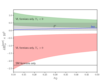
Figure 3: Separate contributions to $\delta R_{\tau\mu}$ in the 4321 model, using the benchmark values in Eqs. (48)–(51), as a function of $x_{Q}$: 1) modified $W$-boson vertex from $U_{1}$+SM fermions (black line), 2) modified $W$-boson vertex from box with one and two VL fermions, for $Y_{+}>0$ (red) or $Y_{+}<0$ (green), 3) $Z^{\prime}$-exchange amplitude (grey band); 4) four-lepton box amplitude (blue line).

To estimate the size of the different contributions to the LFU ratios we choose the following benchmark values for the LQ couplings

$$C_{U}=\frac{g_{U}^{2}v^{2}}{4m_{U}^{2}} =0.01\,,\quad m_{U}=4\ \rm TeV\,,\,$$

$$\beta_{L}^{b\tau} =1,\quad \beta_{L}^{b\mu}=-0.2\,.\quad$$ (48)

These values are representative of the best-fit point obtained in Ref. Cornella:2021sby when fitting present data, in the limit of small RH couplings ($|\beta_{R}^{b\tau}|\ll 1$), and are consistent with the model expectation $W_{ij}=O(1)$ and $|s_{L}|\ll 1$. For the latter reason we further set

$$c_{Q}=1\,,\quad\beta_{L}^{Q\tau}=1,\quad\ \beta^{Q\mu}=-0.2\,.$$ (49)

Given the discussion in Section III.2, we neglect $Y_{-}$ and vary $Y_{+}$ in the interval

$$0.2<|Y_{+}|<1.0~{},$$ (50)

corresponding to $|V_{cb}|<|s_{Q}|<|V_{us}|$. In principle, the signs of $c_{Q}$, $\beta_{L}^{Q\tau}$, and $\beta^{Q\mu}$ could be varied; however, only the relative sign of these couplings and $Y_{+}$ is relevant in $\delta R_{\alpha\beta}$. Therefore we effectively explore all relevant options varying the sign of $Y_{+}$.

Concerning the $Z^{\prime}$ contribution, at fixed $C_{U}$ the result in Eq. (43) depends only on the combination $s_{\tau}^{2}/x_{Z^{\prime}}$. For the sake of simplicity, we set $x_{Z^{\prime}}=3/5$ and vary $s_{\tau}$ in the interval

$$0<s_{\tau}<0.1~{}.$$ (51)

We finally consider the limit of heavy radial excitation, setting $x_{Q}^{R}=x_{Q}/(4\pi)^{2}$.

In Fig. 3 we show all contributions separately in the case of $\delta R_{\tau\mu}$, which is sensitive to all types of amplitudes. As expected, the contribution from $U_{1}$+SM fermions, which includes the LL result, is dominant. However, the contribution from VL fermions represents a significant correction. On the other hand, the $Z^{\prime}$-exchange and the four-lepton box amplitudes are clearly subleading and safely negligible in most of the parameter space.

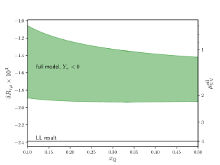
Figure 4: Comparison of the full calculation for $\delta R_{\tau\mu}$ (green band) in the case $Y_{+}<0$, with the LL result obtained using $m_{U}=4$ TeV as UV matching scale (black line). The vertical scale on the right indicates the effective UV matching scale necessary for the LL result to produce a value of $\delta R_{\tau\mu}$ as indicated by the vertical scale on the left.

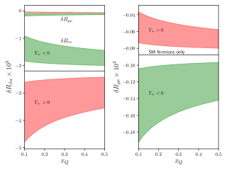
Figure 5: Predictions for $\delta R_{\tau e}$ and $\delta R_{\mu e}$ in the 4321 model, using the benchmark values in Eqs. (48)–(50), as a function of $x_{Q}$. The bands correspond to the full model results. The right plot is a zoom on the upper part of the left plot in order to illustrate the different contributions to $\delta R_{\mu e}$.

In Fig. 4 we compare the LL result for $\delta R_{\tau\mu}$ with the full calculation in the case of $Y_{+}<0$ (and $s_{\tau}=0$), where VL fermions decrease the effect induced by SM fermions only. As expected, in this case the effect is equivalent to that of decreasing the UV matching scale of the the LL result, from its natural value (namely $m_{U}$). The correction is sizable, corresponding to an effective decrease of the matching scale from 4 TeV to about 2 TeV or less. This effect is very relevant in decreasing the present tension with data when fitting the $B$ anomalies Cornella:2021sby .

In Fig. 5 we show the results for both $\delta R_{\tau e}$ and $\delta R_{\mu e}$. As expected, the result for $\delta R_{\tau e}$ is almost identical to that of $\delta R_{\tau\mu}$, whereas the breaking of universality in $\delta R_{\mu e}$ is one order of magnitude smaller, reaching $\mathcal{O}(10^{-4})$ at most. Note that in both cases, the unambiguous predictions following from $B$ anomalies is a reduction of the LFU ratios from one.

VI The effective $W$- and $Z$-boson couplings.

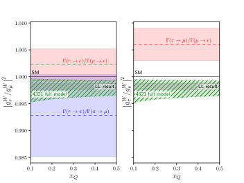
Figure 6: Comparison between data and model predictions for the effective $W$-boson couplings to leptons ($g^{W}_{\ell}$). The hatched green areas indicate the predictions of 4321 models (full model) in the region relevant to the $B$-physics anomalies. The corresponding LL results are highlighted in gray. The red bands are the experimental results obtained using purely leptonic decays Pich:2013lsa . The blue band is the value of $|g^{W}_{\tau}/g^{W}_{\mu}|^{2}$ determined in Ref. Arroyo-Urena:2021nil from $\Gamma(\tau\to\pi\nu)/\Gamma(\pi\to\mu\bar{\nu})$.

The smallness of the $Z^{\prime}$-exchange and the four-lepton box amplitudes allow us to describe the breaking of universality in leptonic $\tau$ decays occurring in 4321 models as modifications of the effective $W$-boson couplings to leptons ($g^{W}_{\ell}$). Defining the latter as

$${\cal{L}}^{(\ell,W)}_{\rm eff}=-{g_{\ell}^{W}\over\sqrt{2}}~{}\overline{\nu}_{\ell}\gamma^{\mu}P_{L}\ell~{}W^{+}_{\mu}+{\rm h.c.},$$ (52)

the ratios introduced in Eq. (1) can be expressed as

$$\left|\frac{g^{(\tau)}_{e}}{g^{(\mu)}_{e}}\right|^{2}\approx\left|\frac{g_{\tau}^{W}}{g_{\mu}^{W}}\right|^{2}~{}.$$ (53)

The smallness of NP effects for one-particle irreducible amplitudes involving the first generation of quarks, implies the same effective $W$-boson couplings can also be extracted from $\Gamma(\tau\to\pi\nu)$ and $\Gamma(\pi\to\mu\bar{\nu})$.

In Fig. 6 we compare our results with the extraction of $|g^{W}_{\tau}/{g^{W}_{\mu}}|$ using both leptonic and pion decays:

$$\left|g_{\tau}^{W}/g_{\mu}^{W}\right|^{2}_{\tau-\rm decays} = 1.0022\pm 0.0030~{}\text{\cite[cite]{\@@bibref{Authors Phrase1YearPhrase2}{Pich:2013lsa}{\@@citephrase{(}}{\@@citephrase{)}}}}\,,$$ (54)

$$\left|g_{\tau}^{W}/g_{\mu}^{W}\right|^{2}_{\pi-\rm decays} = 0.9928\pm 0.0076~{}\text{\cite[cite]{\@@bibref{Authors Phrase1YearPhrase2}{Arroyo-Urena:2021nil}{\@@citephrase{(}}{\@@citephrase{)}}}}\,.$$ (55)

We also compare the model prediction for $|g^{W}_{\tau}/{g^{W}_{e}}|$ with

$$\left|g_{\tau}^{W}/g_{e}^{W}\right|^{2}_{\tau-\rm decays} = 1.0060\pm 0.0030~{}\text{\cite[cite]{\@@bibref{Authors Phrase1YearPhrase2}{Pich:2013lsa}{\@@citephrase{(}}{\@@citephrase{)}}}}\,.$$ (56)

In order to obtain robust estimates, we vary $C_{U}$ in the interval $0.005<C_{U}<0.01$ (with fixed $m_{U}=4$ TeV) and consider both $Y_{+}>0$ and $Y_{+}<0$ (with $s_{\tau}=0$). As can be seen, in the $|g^{W}_{\tau}/{g^{W}_{\mu}}|$ case present data are not precise enough to distinguish the SM from the 4321 model (in the region relevant to the $B$-physics anomalies). In the $|g^{W}_{\tau}/{g^{W}_{e}}|$ case, the inclusion of the contributions from VL fermions decreases the tension with present data, which is reduced to about $2\sigma$ for $Y_{+}<0$. In both cases, a reduction of the present error by a factor 2-3 on the $\tau$ decay widths, which might be accessible at Belle-II, could allow to perform very stringent test of 4321 models in the motivated parameter-space region.

For completeness, we note that in this framework also the left-handed couplings of the $Z$ boson to charged leptons and neutrinos are modified. The calculation proceeds very similarly to the one presented in Section IV for the $W$-boson couplings, the only relevant difference being the presence of the singlet operator $O_{H\ell}^{(1)}$. The corresponding matching conditions reads

$$[C_{H\ell}^{(1)}]_{\tau\tau}(\mu)=\frac{1}{16\pi^{2}}\frac{N_{\rm c}C_{U}}{2}\Big{[}|W_{11}|^{2}|y_{t}|^{2}\left(1+\log\frac{\mu^{2}}{m_{U}^{2}}\right)$$

$$\qquad+c_{Q}^{2}2\text{Re}(W_{11}^{*}W_{21}Y_{+}^{*}y_{t})B_{0}(x_{Q})$$

$$\qquad+c_{Q}^{4}|W_{21}|^{2}(|Y_{+}|^{2}-|Y_{-}|^{2})F(x_{Q},x_{Q}^{R})\Big{]}\,,$$ (57)

$$[C_{H\ell}^{(1)}]_{\mu\mu}(\mu)=\frac{1}{16\pi^{2}}\frac{N_{\rm c}C_{U}}{2}s_{L}^{2}\Big{[}|W_{12}|^{2}|y_{t}|^{2}\left(1+\log\frac{\mu^{2}}{m_{U}^{2}}\right)$$

$$\qquad+c_{Q}^{2}2\text{Re}(W_{12}^{*}W_{22}Y_{+}^{*}y_{t})B_{0}(x_{Q})$$

$$\qquad+c_{Q}^{4}|W_{22}|^{2}(|Y_{+}|^{2}-|Y_{-}|^{2})F(x_{Q},x_{Q}^{R})\Big{]}\,,$$ (58)

while $[C_{H\ell}^{(1)}]_{ee}\approx 0$. Defining the effective left-handed $Z$-boson couplings as

$$\mathcal{L}_{\text{eff}}^{(\ell,Z)}=-\frac{g_{2}}{c_{W}}\left[g_{\ell_{L}}^{Z}(\bar{\ell}\gamma^{\mu}P_{L}\ell)+g_{\nu_{\ell}}^{Z}(\bar{\nu}_{\ell}\gamma^{\mu}P_{L}\nu_{\ell})\right]Z_{\mu}\,,$$ (59)

where $g_{2}$ is the $SU(2)_{L}$ gauge coupling, $c_{W}$ denotes the cosine of the weak angle, and $g^{Z,\text{SM}}_{\nu_{\ell}}=-g^{Z,\text{SM}}_{\ell_{L}}=1/2$, the modified couplings ($g^{Z}_{i}=g^{Z,\text{SM}}_{i}+\delta g^{Z}_{i}$) are

$$\delta g^{Z}_{\nu_{\ell}}(\mu) = -\frac{v^{2}}{2}\left\{[C_{H\ell}^{(1)}]_{\ell\ell}(\mu)-[C_{H\ell}^{(3)}]_{\ell\ell}(\mu)\right\}\,,$$ (60)

$$\delta g^{Z}_{\ell_{L}}(\mu) = -\frac{v^{2}}{2}\left\{[C_{H\ell}^{(1)}]_{\ell\ell}(\mu)+[C_{H\ell}^{(3)}]_{\ell\ell}(\mu)\right\}\,.$$ (61)

Since the leading contributions controlled by $y_{t}$ and $Y_{+}$ are equal and opposite in $C_{H\ell}^{(1)}$ and $C_{H\ell}^{(3)}$, Eqs. (60)–(61) imply a sizable modification of $g^{Z}_{\nu_{\tau}}$ and negligible corrections to all the $g^{Z}_{\ell_{L}}$. Neglecting the subleading contribution proportional to $|Y_{-}|^{2}$ we get

$$\left.\delta g^{Z}_{\ell_{L}}\right|_{Y_{-}=0}=0\,,\quad\left.\frac{\delta g^{Z}_{\nu_{\ell}}}{g^{Z,{\rm SM}}_{\nu_{\ell}}}\right|_{Y_{-}=0}=\left.\frac{\delta g^{W}_{\ell}}{g^{W,{\rm SM}}_{\ell}}\right|_{Y_{-}=0}.$$ (62)

According to this result, the most significant constraint on the model from $Z$-pole observables arises by the invisible decay width of the $Z$-boson, or the effective number of LH neutrinos ($N_{\nu}^{\rm eff}$) determined by this observable ALEPH:2005ab . Assuming that only $\delta g^{Z}_{\nu_{\tau}}$ receives a sizable correction (as expected in our model), we find

$$\left|\frac{g^{Z}_{\nu_{\tau}}}{g^{Z,\rm SM}_{\nu_{\tau}}}\right|^{2}_{N_{\nu}^{\rm eff}}=N_{\nu}^{\rm eff}-2=0.9840\pm 0.0082~{},$$ (63)

which is slightly less stringent than the constraints from the effective $W$ couplings in Eqs. (54)–(56).

VII Conclusion

The recent $B$-physics anomalies have strengthened the importance of precise tests of LFU in all accessible processes involving charged leptons. In this paper we have presented the first complete analysis of LFU violations in leptonic $\tau$ decays, within the motivated class of 4321 models addressing the $B$-physics anomalies DiLuzio:2017vat ; Bordone:2017bld ; Greljo:2018tuh ; DiLuzio:2018zxy ; Fuentes-Martin:2020bnh ; Fuentes-Martin:2020hvc ; Fuentes-Martin:2020pww . As originally pointed out in Ref. Feruglio:2016gvd ; Feruglio:2017rjo via a general EFT approach, the $b\to c\tau\nu$ anomaly implies a decrease of the effective $W$-boson coupling to $\tau$ leptons in the few per-mil range. While confirming this general conclusion, we have shown that the inclusion of vector-like fermions, which is motivated by $B$-physics data in this context, can lead to sizable modifications of the EFT results. In particular, the inclusion of vector-like fermions can partially decrease the present tension of 4321 models with data on leptonic decays. Most importantly, the results presented in this work could lead to very stringent tests for this class of models, in the region favored by $B$-physics data, with the help of future precision measurements of leptonic $\tau$ decay widths.

Acknowledgments

We thank Claudia Cornella and Javier Fuentes-Martín for useful discussions. This project has received funding from the European Research Council (ERC) under the European Union’s Horizon 2020 research and innovation programme under grant agreement 833280 (FLAY), and by the Swiss National Science Foundation (SNF) under contract 200021-175940.

References

- (1) A. Pich, Precision Tau Physics, Prog. Part. Nucl. Phys. 75 (2014) 41 [1310.7922].
- (2) LHCb collaboration, R. Aaij et al., Test of lepton universality in beauty-quark decays, [2103.11769].
- (3) LHCb collaboration, P. de Simone, Experimental Review on Lepton Universality and Lepton Flavour Violation tests in decays, EPJ Web Conf. 234 (2020) 01004.
- (4) A. Greljo, G. Isidori and D. Marzocca, On the breaking of Lepton Flavor Universality in B decays, JHEP 07 (2015) 142 [1506.01705].
- (5) F. Feruglio, P. Paradisi and A. Pattori, Revisiting Lepton Flavor Universality in B Decays, Phys. Rev. Lett. 118 (2017) 011801 [1606.00524].
- (6) F. Feruglio, P. Paradisi and A. Pattori, On the Importance of Electroweak Corrections for B Anomalies, JHEP 09 (2017) 061 [1705.00929].
- (7) E. E. Jenkins, A. V. Manohar and M. Trott, Renormalization Group Evolution of the Standard Model Dimension Six Operators II: Yukawa Dependence, JHEP 01 (2014) 035 [1310.4838].
- (8) L. Di Luzio, A. Greljo and M. Nardecchia, Gauge leptoquark as the origin of B-physics anomalies, Phys. Rev. D 96 (2017) 115011 [1708.08450].
- (9) M. Bordone, C. Cornella, J. Fuentes-Martin and G. Isidori, A three-site gauge model for flavor hierarchies and flavor anomalies, Phys. Lett. B 779 (2018) 317 [1712.01368].
- (10) A. Greljo and B. A. Stefanek, Third family quark–lepton unification at the TeV scale, Phys. Lett. B 782 (2018) 131 [1802.04274].
- (11) L. Di Luzio, J. Fuentes-Martin, A. Greljo, M. Nardecchia and S. Renner, Maximal Flavour Violation: a Cabibbo mechanism for leptoquarks, JHEP 11 (2018) 081 [1808.00942].
- (12) J. Fuentes-Martín and P. Stangl, Third-family quark-lepton unification with a fundamental composite Higgs, Phys. Lett. B 811 (2020) 135953 [2004.11376].
- (13) J. Fuentes-Martín, G. Isidori, M. König and N. Selimović, Vector Leptoquarks Beyond Tree Level III: Vector-like Fermions and Flavor-Changing Transitions, Phys. Rev. D 102 (2020) 115015 [2009.11296].
- (14) J. Fuentes-Martin, G. Isidori, J. Pagès and B. A. Stefanek, Flavor non-universal Pati-Salam unification and neutrino masses, Phys. Lett. B 820 (2021) 136484 [2012.10492].
- (15) R. Barbieri, G. Isidori, A. Pattori and F. Senia, Anomalies in -decays and flavour symmetry, Eur. Phys. J. C 76 (2016) 67 [1512.01560].
- (16) D. Buttazzo, A. Greljo, G. Isidori and D. Marzocca, B-physics anomalies: a guide to combined explanations, JHEP 11 (2017) 044 [1706.07808].
- (17) J. Fuentes-Martín, G. Isidori, M. König and N. Selimović, Vector Leptoquarks Beyond Tree Level, Phys. Rev. D 101 (2020) 035024 [1910.13474].
- (18) J. Fuentes-Martín, G. Isidori, M. König and N. Selimović, Vector leptoquarks beyond tree level. II. corrections and radial modes, Phys. Rev. D 102 (2020) 035021 [2006.16250].
- (19) C. Cornella, D. A. Faroughy, J. Fuentes-Martín, G. Isidori and M. Neubert, Reading the footprints of the B-meson flavor anomalies, [2103.16558].
- (20) E. E. Jenkins, A. V. Manohar and P. Stoffer, Low-Energy Effective Field Theory below the Electroweak Scale: Operators and Matching, JHEP 03 (2018) 016 [1709.04486].
- (21) J. Fuentes-Martín, G. Isidori, J. Pagès and K. Yamamoto, With or without U(2)? Probing non-standard flavor and helicity structures in semileptonic B decays, Phys. Lett. B 800 (2020) 135080 [1909.02519].
- (22) M. A. Arroyo-Ureña, G. Hernández-Tomé, G. López-Castro, P. Roig and I. Rosell, Radiative corrections to : a reliable new physics test, [2107.04603].
- (23) ALEPH, DELPHI, L3, OPAL, SLD, LEP Electroweak Working Group, SLD Electroweak Group, SLD Heavy Flavour Group collaboration, S. Schael et al., Precision electroweak measurements on the resonance, Phys. Rept. 427 (2006) 257 [hep-ex/0509008].