A Three Function Variational Principle for Stationary Non-Barotropic Magnetohydrodynamics

Abstract

Variational principles for magnetohydrodynamics (MHD) were introduced by previous authors both in Lagrangian and Eulerian form. In this paper we introduce simpler Eulerian variational principles from which all the relevant equations of non-barotropic stationary magnetohydrodynamics can be derived for certain field topologies. The variational principle is given in terms of three independent functions for stationary non-barotropic flows. This is a smaller number of variables than the eight variables which appear in the standard equations of non-barotropic magnetohydrodynamics which are the magnetic field $\vec{B}$ the velocity field $\vec{v}$, the entropy $s$ and the density $\rho$. We further investigate the case in the flow along magnetic lines is not ideal.

Keywords: Magnetohydrodynamics, Variational Principles, Reduction of Variables

1 Introduction

Variational principles for magnetohydrodynamics were introduced by previous authors both in Lagrangian and Eulerian form. Sturrock [1] has discussed in his book a Lagrangian variational formalism for magnetohydrodynamics. Vladimirov and Moffatt [2] in a series of papers have discussed an Eulerian variational principle for incompressible magnetohydrodynamics. However, their variational principle contained three more functions in addition to the seven variables which appear in the standard equations of incompressible magnetohydrodynamics which are the magnetic field $\vec{B}$ the velocity field $\vec{v}$ and the pressure $P$. Kats [3] has generalized Moffatt’s work for compressible non barotropic flows but without reducing the number of functions and the computational load. Moreover, Kats has shown that the variables he suggested can be utilized to describe the motion of arbitrary discontinuity surfaces [4, 5]. Sakurai [6] has introduced a two function Eulerian variational principle for force-free magnetohydrodynamics and used it as a basis of a numerical scheme, his method is discussed in a book by Sturrock [1]. A method of solving the equations for those two variables was introduced by Yang, Sturrock & Antiochos [8]. Yahalom & Lynden-Bell [9] combined the Lagrangian of Sturrock [1] with the Lagrangian of Sakurai [6] to obtain an Eulerian Lagrangian principle for barotropic magnetohydrodynamics which will depend on only six functions. The variational derivative of this Lagrangian produced all the equations needed to describe barotropic magnetohydrodynamics without any additional constraints. The equations obtained resembled the equations of Frenkel, Levich & Stilman [12] (see also [13]). Yahalom [10] have shown that for the barotropic case four functions will suffice. Moreover, it was shown that the cuts of some of those functions [11] are topological local conserved quantities.

Previous work was concerned only with barotropic magnetohydrodynamics. Variational principles of non barotropic magnetohydrodynamics can be found in the work of Bekenstein & Oron [14] in terms of 15 functions and V.A. Kats [3] in terms of 20 functions. The author of this paper suspect that this number can be somewhat reduced. Moreover, A. V. Kats in a remarkable paper [15] (section IV,E) has shown that there is a large symmetry group (gauge freedom) associated with the choice of those functions, this implies that the number of degrees of freedom can be reduced. Yahalom [16, 17] have shown that only five functions will suffice to describe non barotropic magnetohydrodynamics in the case that we enforce a Sakurai [6] representation for the magnetic field. Morrison [7] has suggested a Hamiltonian approach but this also depends on 8 canonical variables (see table 2 [7]). The work of Yahalom [16] was concerned with general non-stationary flows. In a separate work [18] was concerned with stationary flows and introduced a 8 variable stationary variational principle, here we shall attempt to improve on this and obtain a 3 variable stationary variational principle for non-barotropic MHD. This will be done for a general case in which the magnetic field lines need not lie on entropy surfaces, for the restricted case in which the magnetic field lines lie on entropy surfaces see [19].

We anticipate applications of this study both to linear and non-linear stability analysis of known non barotropic magnetohydrodynamic configurations [26, 28] and for designing efficient numerical schemes for integrating the equations of fluid dynamics and magnetohydrodynamics [34, 35, 37]. Another possible application is connected to obtaining new analytic solutions in terms of the variational variables [38].

The plan of this paper is as follows: First we introduce the standard notations and equations of non-barotropic magnetohydrodynamics for the stationary and non-stationary cases. Then we introduce the concepts of load and metage. The variational principle follows.

2 Standard formulation of non-barotropic magnetohydrodynamics

The standard set of equations solved for non-barotropic magnetohydrodynamics are given below:

$$\frac{\partial{\vec{B}}}{\partial t}=\vec{\nabla}\times(\vec{v}\times\vec{B}),$$ (1)

$$\vec{\nabla}\cdot\vec{B}=0,$$ (2)

$$\frac{\partial{\rho}}{\partial t}+\vec{\nabla}\cdot(\rho\vec{v})=0,$$ (3)

$$\rho\frac{d\vec{v}}{dt}=\rho(\frac{\partial\vec{v}}{\partial t}+(\vec{v}\cdot\vec{\nabla})\vec{v})=-\vec{\nabla}p(\rho,s)+\frac{(\vec{\nabla}\times\vec{B})\times\vec{B}}{4\pi}.$$ (4)

$$\frac{ds}{dt}=0.$$ (5)

The following notations are utilized: $\frac{\partial}{\partial t}$ is the temporal derivative, $\frac{d}{dt}$ is the temporal material derivative and $\vec{\nabla}$ has its standard meaning in vector calculus. $\vec{B}$ is the magnetic field vector, $\vec{v}$ is the velocity field vector, $\rho$ is the fluid density and $s$ is the specific entropy. Finally $p(\rho,s)$ is the pressure which depends on the density and entropy (the non-barotropic case).

The justification for those equations and the conditions under which they apply can be found in standard books on magnetohydrodynamics (see for example [1]). The above applies to a collision-dominated plasma in local thermodynamic equilibrium. Such conditions are seldom satisfied by physical plasmas, certainly not in astrophysics or in fusion-relevant magnetic confinement experiments. Never the less it is believed that the fastest macroscopic instabilities in those systems obey the above equations [11], while instabilities associated with viscous or finite conductivity terms are slower. It should be noted that due to a theorem by Bateman [39] every physical system can be described by a variational principle (including viscous plasma) the trick is to find an elegant variational principle usually depending on a small amount of variational variables. The current work will discuss only ideal magnetohydrodynamics while viscous magnetohydrodynamics will be left for future endeavors.

Equation (1) describes the fact that the magnetic field lines are moving with the fluid elements (”frozen” magnetic field lines), equation (2) describes the fact that the magnetic field is solenoidal, equation (3) describes the conservation of mass and equation (4) is the Euler equation for a fluid in which both pressure and Lorentz magnetic forces apply. The term:

$$\vec{J}=\frac{\vec{\nabla}\times\vec{B}}{4\pi},$$ (6)

is the electric current density which is not connected to any mass flow. Equation (5) describes the fact that heat is not created (zero viscosity, zero resistivity) in ideal non-barotropic magnetohydrodynamics and is not conducted, thus only convection occurs. The number of independent variables for which one needs to solve is eight ($\vec{v},\vec{B},\rho,s$) and the number of equations (1,3,4,5) is also eight. Notice that equation (2) is a condition on the initial $\vec{B}$ field and is satisfied automatically for any other time due to equation (1). For the stationary case in which the physical fields do not depend on time we obtain the following set of stationary equations:

$$\vec{\nabla}\times(\vec{v}\times\vec{B})=0,$$ (7)

$$\vec{\nabla}\cdot\vec{B}=0,$$ (8)

$$\vec{\nabla}\cdot(\rho\vec{v})=0,$$ (9)

$$\rho(\vec{v}\cdot\vec{\nabla})\vec{v}=-\vec{\nabla}p(\rho,s)+\frac{(\vec{\nabla}\times\vec{B})\times\vec{B}}{4\pi}.$$ (10)

$$\vec{v}\cdot\vec{\nabla}s=0.$$ (11)

3 Variational principle of non-barotropic magnetohydrodynamics

In the following section we will generalize the approach of [9] for the non-barotropic case. Consider the action:

$$A \equiv \int{\cal L}d^{3}xdt,$$

$${\cal L} \equiv {\cal L}_{1}+{\cal L}_{2},$$

$${\cal L}_{1} \equiv \rho(\frac{1}{2}\vec{v}^{2}-\varepsilon(\rho,s))+\frac{\vec{B}^{2}}{8\pi},$$

$${\cal L}_{2} \equiv \nu[\frac{\partial{\rho}}{\partial t}+\vec{\nabla}\cdot(\rho\vec{v})]-\rho\alpha\frac{d\chi}{dt}-\rho\beta\frac{d\eta}{dt}-\rho\sigma\frac{ds}{dt}$$ (12)

$$- \frac{\vec{B}}{4\pi}\cdot\vec{\nabla}\chi\times\vec{\nabla}\eta.$$

In the above $\varepsilon$ is the specific internal energy (internal energy per unit of mass). The reader is reminded of the following thermodynamic relations which will become useful later:

$$d\varepsilon = Tds-Pd\frac{1}{\rho}=Tds+\frac{P}{\rho^{2}}d\rho$$

$$\frac{\partial\varepsilon}{\partial s}=T,\qquad\frac{\partial\varepsilon}{\partial\rho}=\frac{P}{\rho^{2}}$$

$$w = \varepsilon+\frac{P}{\rho}=\varepsilon+\frac{\partial\varepsilon}{\partial\rho}\rho=\frac{\partial(\rho\varepsilon)}{\partial\rho}$$

$$dw = d\varepsilon+d(\frac{P}{\rho})=Tds+\frac{1}{\rho}dP$$ (13)

in the above $T$ is the temperature and $w$ is the specific enthalpy. in the above: $\varepsilon$ is the specific internal energy, $T$ is the temperature and $w$ is the specific enthalpy. A special case of equation of state is the polytropic equation of state [42]:

$$p=K\rho^{\gamma}$$ (14)

$K$ and $\gamma$ may depend on the specific entropy $s$. Hence:

$$\frac{\partial\varepsilon}{\partial\rho}=K\rho^{\gamma-2}\Rightarrow\varepsilon=\frac{K}{\gamma-1}\rho^{\gamma-1}=\frac{p}{\rho(\gamma-1)}\Rightarrow\rho\varepsilon=\frac{p}{\gamma-1}$$ (15)

the last identity is up to a function dependent on $s$. Obviously $\nu,\alpha,\beta,\sigma$ are Lagrange multipliers which were inserted in such a way that the variational principle will yield the following equations:

$$\frac{\partial{\rho}}{\partial t}+\vec{\nabla}\cdot(\rho\vec{v})=0,$$

$$\rho\frac{d\chi}{dt}=0,$$

$$\rho\frac{d\eta}{dt}=0.$$

$$\rho\frac{ds}{dt}=0.$$ (16)

It is not assumed that $\nu,\alpha,\beta,\sigma$ are single valued. Provided $\rho$ is not null those are just the continuity equation (3), entropy conservation and the conditions that Sakurai’s functions are comoving. Taking the variational derivative with respect to $\vec{B}$ we see that

$$\vec{B}=\hat{\vec{B}}\equiv\vec{\nabla}\chi\times\vec{\nabla}\eta.$$ (17)

Hence $\vec{B}$ is in Sakurai’s form and satisfies equation (2). It can be easily shown that provided that $\vec{B}$ is in the form given in equation (17), and equations (16) are satisfied, then also equation (1) is satisfied.

For the time being we have showed that all the equations of non-barotropic magnetohydrodynamics can be obtained from the above variational principle except Euler’s equations. We will now show that Euler’s equations can be derived from the above variational principle as well. Let us take an arbitrary variational derivative of the above action with respect to $\vec{v}$, this will result in:

$$\delta_{\vec{v}}A = \int dt\{\int d^{3}xdt\rho\delta\vec{v}\cdot[\vec{v}-\vec{\nabla}\nu-\alpha\vec{\nabla}\chi-\beta\vec{\nabla}\eta-\sigma\vec{\nabla}s]$$ (18)

$$+ \oint d\vec{S}\cdot\delta\vec{v}\rho\nu+\int d\vec{\Sigma}\cdot\delta\vec{v}\rho[\nu]\}.$$

The integral $\oint d\vec{S}\cdot\delta\vec{v}\rho\nu$ vanishes in many physical scenarios. In the case of astrophysical flows this integral will vanish since $\rho=0$ on the flow boundary, in the case of a fluid contained in a vessel no flux boundary conditions $\delta\vec{v}\cdot\hat{n}=0$ are induced ($\hat{n}$ is a unit vector normal to the boundary). The surface integral $\int d\vec{\Sigma}$ on the cut of $\nu$ vanishes in the case that $\nu$ is single valued and $[\nu]=0$ as is the case for some flow topologies. In the case that $\nu$ is not single valued only a Kutta type velocity perturbation [36] in which the velocity perturbation is parallel to the cut will cause the cut integral to vanish. An arbitrary velocity perturbation on the cut will indicate that $\rho=0$ on this surface which is contradictory to the fact that a cut surface is to some degree arbitrary as is the case for the zero line of an azimuthal angle. We will show later that the ”cut” surface is co-moving with the flow hence it may become quite complicated. This uneasy situation may be somewhat be less restrictive when the flow has some symmetry properties.

Provided that the surface integrals do vanish and that $\delta_{\vec{v}}A=0$ for an arbitrary velocity perturbation we see that $\vec{v}$ must have the following form:

$$\vec{v}=\hat{\vec{v}}\equiv\vec{\nabla}\nu+\alpha\vec{\nabla}\chi+\beta\vec{\nabla}\eta+\sigma\vec{\nabla}s.$$ (19)

The above equation is reminiscent of Clebsch representation in non magnetic fluids [43, 44]. Let us now take the variational derivative with respect to the density $\rho$ we obtain:

$$\delta_{\rho}A = \int d^{3}xdt\delta\rho[\frac{1}{2}\vec{v}^{2}-w-\frac{\partial{\nu}}{\partial t}-\vec{v}\cdot\vec{\nabla}\nu]$$ (20)

$$+ \int dt\oint d\vec{S}\cdot\vec{v}\delta\rho\nu+\int dt\int d\vec{\Sigma}\cdot\vec{v}\delta\rho[\nu]$$

$$+ \int d^{3}x\nu\delta\rho|^{t_{1}}_{t_{0}}.$$

In which $w=\frac{\partial(\varepsilon\rho)}{\partial\rho}$ is the specific enthalpy. Hence provided that $\oint d\vec{S}\cdot\vec{v}\delta\rho\nu$ vanishes on the boundary of the domain and $\int d\vec{\Sigma}\cdot\vec{v}\delta\rho[\nu]$ vanishes on the cut of $\nu$ in the case that $\nu$ is not single valued and in initial and final times the following equation must be satisfied:

$$\frac{d\nu}{dt}=\frac{1}{2}\vec{v}^{2}-w,\qquad$$ (21)

Since the right hand side of the above equation is single valued as it is made of physical quantities, we conclude that:

$$\frac{d[\nu]}{dt}=0.$$ (22)

Hence the cut value is co-moving with the flow and thus the cut surface may become arbitrary complicated. This uneasy situation may be somewhat be less restrictive when the flow has some symmetry properties.

Finally we have to calculate the variation with respect to both $\chi$ and $\eta$ this will lead us to the following results:

$$\delta_{\chi}A = \int d^{3}xdt\delta\chi[\frac{\partial{(\rho\alpha)}}{\partial t}+\vec{\nabla}\cdot(\rho\alpha\vec{v})-\vec{\nabla}\eta\cdot\vec{J}]$$ (23)

$$+ \int dt\oint d\vec{S}\cdot[\frac{\vec{B}}{4\pi}\times\vec{\nabla}\eta-\vec{v}\rho\alpha]\delta\chi$$

$$+ \int dt\int d\vec{\Sigma}\cdot[\frac{\vec{B}}{4\pi}\times\vec{\nabla}\eta-\vec{v}\rho\alpha][\delta\chi]$$

$$- \int d^{3}x\rho\alpha\delta\chi|^{t_{1}}_{t_{0}},$$

$$\delta_{\eta}A = \int d^{3}xdt\delta\eta[\frac{\partial{(\rho\beta)}}{\partial t}+\vec{\nabla}\cdot(\rho\beta\vec{v})+\vec{\nabla}\chi\cdot\vec{J}]$$ (24)

$$+ \int dt\oint d\vec{S}\cdot[\vec{\nabla}\chi\times\frac{\vec{B}}{4\pi}-\vec{v}\rho\beta]\delta\eta$$

$$+ \int dt\int d\vec{\Sigma}\cdot[\vec{\nabla}\chi\times\frac{\vec{B}}{4\pi}-\vec{v}\rho\beta][\delta\eta]$$

$$- \int d^{3}x\rho\beta\delta\eta|^{t_{1}}_{t_{0}}.$$

Provided that the correct temporal and boundary conditions are met with respect to the variations $\delta\chi$ and $\delta\eta$ on the domain boundary and on the cuts in the case that some (or all) of the relevant functions are non single valued. we obtain the following set of equations:

$$\frac{d\alpha}{dt}=\frac{\vec{\nabla}\eta\cdot\vec{J}}{\rho},\qquad\frac{d\beta}{dt}=-\frac{\vec{\nabla}\chi\cdot\vec{J}}{\rho},$$ (25)

in which the continuity equation (3) was taken into account. By correct temporal conditions we mean that both $\delta\eta$ and $\delta\chi$ vanish at initial and final times. As for boundary conditions which are sufficient to make the boundary term vanish on can consider the case that the boundary is at infinity and both $\vec{B}$ and $\rho$ vanish. Another possibility is that the boundary is impermeable and perfectly conducting. A sufficient condition for the integral over the ”cuts” to vanish is to use variations $\delta\eta$ and $\delta\chi$ which are single valued. It can be shown that $\chi$ can always be taken to be single valued, hence taking $\delta\chi$ to be single valued is no restriction at all. In some topologies $\eta$ is not single valued and in those cases a single valued restriction on $\delta\eta$ is sufficient to make the cut term null.

Finally we take a variational derivative with respect to the entropy $s$:

$$\delta_{s}A = \int d^{3}xdt\delta s[\frac{\partial{(\rho\sigma)}}{\partial t}+\vec{\nabla}\cdot(\rho\sigma\vec{v})-\rho T]$$ (26)

$$+ \int dt\oint d\vec{S}\cdot\rho\sigma\vec{v}\delta s-\int d^{3}x\rho\sigma\delta s|^{t_{1}}_{t_{0}},$$

in which the temperature is $T=\frac{\partial\varepsilon}{\partial s}$. We notice that according to equation (19) $\sigma$ is single valued and hence no cuts are needed. Taking into account the continuity equation (3) we obtain for locations in which the density $\rho$ is not null the result:

$$\frac{d\sigma}{dt}=T,$$ (27)

provided that $\delta_{s}A$ vanished for an arbitrary $\delta s$.

4 Euler’s equations

We shall now show that a velocity field given by equation (19), such that the equations for $\alpha,\beta,\chi,\eta,\nu,\sigma,s$ satisfy the corresponding equations (16,21,25,27) must satisfy Euler’s equations. Let us calculate the material derivative of $\vec{v}$:

$$\frac{d\vec{v}}{dt} = \frac{d\vec{\nabla}\nu}{dt}+\frac{d\alpha}{dt}\vec{\nabla}\chi+\alpha\frac{d\vec{\nabla}\chi}{dt}+\frac{d\beta}{dt}\vec{\nabla}\eta+\beta\frac{d\vec{\nabla}\eta}{dt}$$ (28)

$$+ \frac{d\sigma}{dt}\vec{\nabla}s+\sigma\frac{d\vec{\nabla}s}{dt}.$$

It can be easily shown that:

$$\frac{d\vec{\nabla}\nu}{dt} = \vec{\nabla}\frac{d\nu}{dt}-\vec{\nabla}v_{k}\frac{\partial\nu}{\partial x_{k}}=\vec{\nabla}(\frac{1}{2}\vec{v}^{2}-w)-\vec{\nabla}v_{k}\frac{\partial\nu}{\partial x_{k}},$$

$$\frac{d\vec{\nabla}\eta}{dt} = \vec{\nabla}\frac{d\eta}{dt}-\vec{\nabla}v_{k}\frac{\partial\eta}{\partial x_{k}}=-\vec{\nabla}v_{k}\frac{\partial\eta}{\partial x_{k}},$$

$$\frac{d\vec{\nabla}\chi}{dt} = \vec{\nabla}\frac{d\chi}{dt}-\vec{\nabla}v_{k}\frac{\partial\chi}{\partial x_{k}}=-\vec{\nabla}v_{k}\frac{\partial\chi}{\partial x_{k}},$$

$$\frac{d\vec{\nabla}s}{dt} = \vec{\nabla}\frac{ds}{dt}-\vec{\nabla}v_{k}\frac{\partial s}{\partial x_{k}}=-\vec{\nabla}v_{k}\frac{\partial s}{\partial x_{k}}.$$ (29)

In which $x_{k}$ is a Cartesian coordinate and a summation convention is assumed. Inserting the result from equations (29,16) into equation (28) yields:

$$\frac{d\vec{v}}{dt} = -\vec{\nabla}v_{k}(\frac{\partial\nu}{\partial x_{k}}+\alpha\frac{\partial\chi}{\partial x_{k}}+\beta\frac{\partial\eta}{\partial x_{k}}+\sigma\frac{\partial s}{\partial x_{k}})$$ (30)

$$+ \vec{\nabla}(\frac{1}{2}\vec{v}^{2}-w)+T\vec{\nabla}s$$

$$+ \frac{1}{\rho}((\vec{\nabla}\eta\cdot\vec{J})\vec{\nabla}\chi-(\vec{\nabla}\chi\cdot\vec{J})\vec{\nabla}\eta)$$

$$= -\vec{\nabla}v_{k}v_{k}+\vec{\nabla}(\frac{1}{2}\vec{v}^{2}-w)+T\vec{\nabla}s$$

$$+ \frac{1}{\rho}\vec{J}\times(\vec{\nabla}\chi\times\vec{\nabla}\eta)$$

$$= -\frac{\vec{\nabla}p}{\rho}+\frac{1}{\rho}\vec{J}\times\vec{B}.$$

In which we have used both equation (19) and equation (17) in the above derivation. This of course proves that the non-barotropic Euler equations can be derived from the action given in equation (12) and hence all the equations of non-barotropic magnetohydrodynamics can be derived from the above action without restricting the variations in any way except on the relevant boundaries and cuts.

5 Simplified action

The reader of this paper might argue here that the paper is misleading. The author has declared that he is going to present a simplified action for non-barotropic magnetohydrodynamics instead he added six more functions $\alpha,\beta,\chi,\-\eta,\nu,\sigma$ to the standard set $\vec{B},\vec{v},\rho,s$. In the following I will show that this is not so and the action given in equation (12) in a form suitable for a pedagogic presentation can indeed be simplified. It is easy to show that the Lagrangian density appearing in equation (12) can be written in the form:

$${\cal L} = -\rho[\frac{\partial{\nu}}{\partial t}+\alpha\frac{\partial{\chi}}{\partial t}+\beta\frac{\partial{\eta}}{\partial t}+\sigma\frac{\partial{s}}{\partial t}+\varepsilon(\rho,s)]$$ (31)

$$+ \frac{1}{2}\rho[(\vec{v}-\hat{\vec{v}})^{2}-(\hat{\vec{v}})^{2}]$$

$$+ \frac{1}{8\pi}[(\vec{B}-\hat{\vec{B}})^{2}-(\hat{\vec{B}})^{2}]+\frac{\partial{(\nu\rho)}}{\partial t}+\vec{\nabla}\cdot(\nu\rho\vec{v}).$$

In which $\hat{\vec{v}}$ is a shorthand notation for $\vec{\nabla}\nu+\alpha\vec{\nabla}\chi+\beta\vec{\nabla}\eta+\sigma\vec{\nabla}s$ (see equation (19)) and $\hat{\vec{B}}$ is a shorthand notation for $\vec{\nabla}\chi\times\vec{\nabla}\eta$ (see equation (17)). Thus ${\cal L}$ has four contributions:

$${\cal L} = \hat{\cal L}+{\cal L}_{\vec{v}}+{\cal L}_{\vec{B}}+{\cal L}_{boundary},$$

$$\hat{\cal L} \equiv -\rho\left[\frac{\partial{\nu}}{\partial t}+\alpha\frac{\partial{\chi}}{\partial t}+\beta\frac{\partial{\eta}}{\partial t}+\sigma\frac{\partial{s}}{\partial t}\right.$$

$$+ \left.\varepsilon(\rho,s)+\frac{1}{2}(\vec{\nabla}\nu+\alpha\vec{\nabla}\chi+\beta\vec{\nabla}\eta+\sigma\vec{\nabla}s)^{2}\right]$$

$$- \frac{1}{8\pi}(\vec{\nabla}\chi\times\vec{\nabla}\eta)^{2}$$

$${\cal L}_{\vec{v}} \equiv \frac{1}{2}\rho(\vec{v}-\hat{\vec{v}})^{2},$$

$${\cal L}_{\vec{B}} \equiv \frac{1}{8\pi}(\vec{B}-\hat{\vec{B}})^{2},$$

$${\cal L}_{boundary} \equiv \frac{\partial{(\nu\rho)}}{\partial t}+\vec{\nabla}\cdot(\nu\rho\vec{v}).$$ (32)

The only term containing $\vec{v}$ is ${\cal L}_{\vec{v}}$, it can easily be seen that this term will lead, after we nullify the variational derivative with respect to $\vec{v}$, to equation (19) but will otherwise have no contribution to other variational derivatives. Similarly the only term containing $\vec{B}$ is ${\cal L}_{\vec{B}}$ and it can easily be seen that this term will lead, after we nullify the variational derivative, to equation (17) but will have no contribution to other variational derivatives. Also notice that the term ${\cal L}_{boundary}$ contains only complete partial derivatives and thus can not contribute to the equations although it can change the boundary conditions. Hence we see that equations (16), equation (21), equations (25) and equation (27) can be derived using the Lagrangian density:

$$\hat{\cal L}[\alpha,\beta,\chi,\eta,\nu,\rho,\sigma,s]=-\rho[\frac{\partial{\nu}}{\partial t}+\alpha\frac{\partial{\chi}}{\partial t}+\beta\frac{\partial{\eta}}{\partial t}+\sigma\frac{\partial{s}}{\partial t}$$ (33)

$$+ \varepsilon(\rho,s)+\frac{1}{2}(\vec{\nabla}\nu+\alpha\vec{\nabla}\chi+\beta\vec{\nabla}\eta+\sigma\vec{\nabla}s)^{2}]$$

$$- \frac{1}{8\pi}(\vec{\nabla}\chi\times\vec{\nabla}\eta)^{2}$$

in which $\hat{\vec{v}}$ replaces $\vec{v}$ and $\hat{\vec{B}}$ replaces $\vec{B}$ in the relevant equations. Furthermore, after integrating the eight equations (16,21,25,27) we can insert the potentials $\alpha,\beta,\chi,\eta,\nu,\sigma,s$ into equations (19) and (17) to obtain the physical quantities $\vec{v}$ and $\vec{B}$. Hence, the general non-barotropic magnetohydrodynamic problem is reduced from eight equations (1,3,4,5) and the additional constraint (2) to a problem of eight first order (in the temporal derivative) unconstrained equations. Moreover, the entire set of equations can be derived from the Lagrangian density $\hat{\cal L}$.

6 Stationary non-barotropic MHD

Stationary flows are a unique phenomena of Eulerian fluid dynamics which has no counter part in Lagrangian fluid dynamics. The stationary flow is defined by the fact that the physical fields $\vec{v},\vec{B},\rho,s$ do not depend on the temporal coordinate. This, however, does not imply that the corresponding potentials $\alpha,\beta,\chi,\eta,\nu,\sigma$ are all functions of spatial coordinates alone. Moreover, it can be shown that choosing the potentials in such a way will lead to erroneous results in the sense that the stationary equations of motion can not be derived from the Lagrangian density $\hat{\cal L}$ given in equation (32). However, this problem can be amended easily as follows. Let us choose $\alpha,\beta,\chi,\nu,\sigma$ to depend on the spatial coordinates alone. Let us choose $\eta$ such that:

$$\eta=\bar{\eta}-t,$$ (34)

in which $\bar{\eta}$ is a function of the spatial coordinates. The Lagrangian density $\hat{\cal L}$ given in equation (32) will take the form:

$$\hat{\cal L} = \rho(\beta-\varepsilon(\rho,s))-\frac{1}{2}\rho(\vec{\nabla}\nu+\alpha\vec{\nabla}\chi+\beta\vec{\nabla}\bar{\eta}+\sigma\vec{\nabla}s)^{2}$$ (35)

$$- \frac{1}{8\pi}(\vec{\nabla}\chi\times\vec{\nabla}\bar{\eta})^{2}.$$

The above functional can be compared with Vladimirov and Moffatt [2] equation 6.12 for incompressible flows in which their $I$ is analogue to our $\beta$. Notice however, that while $\beta$ is not a conserved quantity $I$ is.

Varying the Lagrangian $\hat{L}=\int\hat{\cal L}d^{3}x$ with respect to $\nu,\alpha,\beta,\chi,\eta,\rho,\sigma,s$ leads to the following equations:

$$\vec{\nabla}\cdot(\rho\hat{\vec{v}})=0,$$

$$\rho\hat{\vec{v}}\cdot\vec{\nabla}\chi=0,$$

$$\rho(\hat{\vec{v}}\cdot\vec{\nabla}\bar{\eta}-1)=0,$$

$$\hat{\vec{v}}\cdot\vec{\nabla}\alpha=\frac{\vec{\nabla}\bar{\eta}\cdot\hat{\vec{J}}}{\rho},\qquad$$

$$\hat{\vec{v}}\cdot\vec{\nabla}\beta=-\frac{\vec{\nabla}\chi\cdot\hat{\vec{J}}}{\rho},$$

$$\beta=\frac{1}{2}\hat{\vec{v}}^{2}+w,$$

$$\rho\hat{\vec{v}}\cdot\vec{\nabla}s=0,$$

$$\rho\hat{\vec{v}}\cdot\vec{\nabla}\sigma=\rho T.$$ (36)

Calculations similar to the ones done in previous subsections will show that those equations lead to the stationary non-barotropic magnetohydrodynamic equations:

$$\vec{\nabla}\times(\hat{\vec{v}}\times\hat{\vec{B}})=0,$$ (37)

$$\rho(\hat{\vec{v}}\cdot\vec{\nabla})\hat{\vec{v}}=-\vec{\nabla}p(\rho,s)+\frac{(\vec{\nabla}\times\hat{\vec{B}})\times\hat{\vec{B}}}{4\pi}.$$ (38)

In what follows we will attempt to reduce the number of variational variables from eight to four.

7 Load and Metage

The following section follows closely a similar section in [9]. Consider a thin tube surrounding a magnetic field line as described in figure 1,

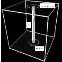
Figure 1: A thin tube surrounding a magnetic field line

the magnetic flux contained within the tube is:

$$\Delta\Phi=\int\vec{B}\cdot d\vec{S}$$ (39)

and the mass contained with the tube is:

$$\Delta M=\int\rho d\vec{l}\cdot d\vec{S},$$ (40)

in which $dl$ is a length element along the tube. Since the magnetic field lines move with the flow by virtue of equation (1) and equation (3) both the quantities $\Delta\Phi$ and $\Delta M$ are conserved and since the tube is thin we may define the conserved magnetic load:

$$\lambda=\frac{\Delta M}{\Delta\Phi}=\oint\frac{\rho}{B}dl,$$ (41)

in which the above integral is performed along the field line. Obviously the parts of the line which go out of the flow to regions in which $\rho=0$ have a null contribution to the integral. Notice that $\lambda$ is a single valued function that can be measured in principle. Since $\lambda$ is conserved it satisfies the equation:

$$\frac{d\lambda}{dt}=0.$$ (42)

By construction surfaces of constant magnetic load move with the flow and contain magnetic field lines. Hence the gradient to such surfaces must be orthogonal to the field line:

$$\vec{\nabla}\lambda\cdot\vec{B}=0.$$ (43)

Now consider an arbitrary comoving point on the magnetic field line and denote it by $i$, and consider an additional comoving point on the magnetic field line and denote it by $r$. The integral:

$$\mu(r)=\int_{i}^{r}\frac{\rho}{B}dl+\mu(i),$$ (44)

is also a conserved quantity which we may denote following Lynden-Bell & Katz [20] as the magnetic metage. $\mu(i)$ is an arbitrary number which can be chosen differently for each magnetic line. By construction:

$$\frac{d\mu}{dt}=0.$$ (45)

Also it is easy to see that by differentiating along the magnetic field line we obtain:

$$\vec{\nabla}\mu\cdot\vec{B}=\rho.$$ (46)

Notice that $\mu$ will be generally a non single valued function, we will show later in this paper that symmetry to translations in $\mu$ will generate through the Noether theorem the conservation of the magnetic cross helicity.

At this point we have two comoving coordinates of flow, namely $\lambda,\mu$ obviously in a three dimensional flow we also have a third coordinate. However, before defining the third coordinate we will find it useful to work not directly with $\lambda$ but with a function of $\lambda$. Now consider the magnetic flux within a surface of constant load $\Phi(\lambda)$ as described in figure 2

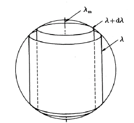
Figure 2: Surfaces of constant load

(the figure was given by Lynden-Bell & Katz [20]). The magnetic flux is a conserved quantity and depends only on the load $\lambda$ of the surrounding surface. Now we define the quantity:

$$\chi=\frac{\Phi(\lambda)}{2\pi}.$$ (47)

Obviously $\chi$ satisfies the equations:

$$\frac{d\chi}{dt}=0,\qquad\vec{B}\cdot\vec{\nabla}\chi=0.$$ (48)

Let us now define an additional comoving coordinate $\eta^{*}$ since $\vec{\nabla}\mu$ is not orthogonal to the $\vec{B}$ lines we can choose $\vec{\nabla}\eta^{*}$ to be orthogonal to the $\vec{B}$ lines and not be in the direction of the $\vec{\nabla}\chi$ lines, that is we choose $\eta^{*}$ not to depend only on $\chi$. Since both $\vec{\nabla}\eta^{*}$ and $\vec{\nabla}\chi$ are orthogonal to $\vec{B}$, $\vec{B}$ must take the form:

$$\vec{B}=A\vec{\nabla}\chi\times\vec{\nabla}\eta^{*}.$$ (49)

However, using equation (2) we have:

$$\vec{\nabla}\cdot\vec{B}=\vec{\nabla}A\cdot(\vec{\nabla}\chi\times\vec{\nabla}\eta^{*})=0.$$ (50)

Which implies that $A$ is a function of $\chi,\eta^{*}$. Now we can define a new comoving function $\eta$ such that:

$$\eta=\int_{0}^{\eta^{*}}A(\chi,\eta^{{}^{\prime}*})d\eta^{{}^{\prime}*},\qquad\frac{d\eta}{dt}=0.$$ (51)

In terms of this function we obtain the Sakurai (Euler potentials) presentation:

$$\vec{B}=\vec{\nabla}\chi\times\vec{\nabla}\eta.$$ (52)

Hence we have shown how $\chi,\eta$ can be constructed for a known $\vec{B},\rho$. Notice however, that $\eta$ is defined in a non unique way since one can redefine $\eta$ for example by performing the following transformation: $\eta\rightarrow\eta+f(\chi)$ in which $f(\chi)$ is an arbitrary function. The comoving coordinates $\chi,\eta$ serve as labels of the magnetic field lines. Moreover the magnetic flux can be calculated as:

$$\Phi=\int\vec{B}\cdot d\vec{S}=\int d\chi d\eta.$$ (53)

In the case that the surface integral is performed inside a load contour we obtain:

$$\Phi(\lambda)=\int_{\lambda}d\chi d\eta=\chi\int_{\lambda}d\eta=\left\{\begin{array}[]{c}\chi[\eta]\\ \chi(\eta_{max}-\eta_{min})\\ \end{array}\right.$$ (54)

There are two cases involved; in one case the load surfaces are topological cylinders, in this case $\eta$ is not single valued and hence we obtain the upper value for $\Phi(\lambda)$. In a second case the load surfaces are topological spheres, in this case $\eta$ is single valued and has minimal $\eta_{min}$ and maximal $\eta_{max}$ values. Hence the lower value of $\Phi(\lambda)$ is obtained. For example in some cases $\eta$ is identical to twice the latitude angle $\theta$. In those cases $\eta_{min}=0$ (value at the ”north pole”) and $\eta_{max}=2\pi$ (value at the ”south pole”).

Comparing the above equation with equation (47) we derive that $\eta$ can be either single valued or not single valued and that its discontinuity across its cut in the non single valued case is $[\eta]=2\pi$.

So far the discussion did not differentiate the cases of stationary and non-stationary flows. It should be noted that even for stationary flows one can have a non-stationary $\eta$ coordinates as the magnetic field depends only on the gradient of $\eta$ (see equation (52)), in particular if $\eta$ is stationary than $\eta+g(t)$ which is clearly not stationary will produce according to equation (52) a stationary magnetic field. In what follows we find it advantageous to use the form of $\eta$ given in equation (34) in which $\bar{\eta}$ is stationary.

The triplet $\chi,\eta,\mu$ will suffice to label any fluid element in three dimensions. But for a non-barotropic flow there is also another possible label $s$ which is comoving according to equation (5). The question then arises of the relation of this label to the previous three. As one needs to make a choice regarding the preferred set of labels it seems that the physical ones are $\chi,\eta,s$ in which we use the surfaces on which the magnetic fields lie and the entropy, each label has an obvious physical interpretation. In this case we must look at $\mu$ as a function of $\chi,\eta,s$. If the magnetic field lines lie on entropy surface then $\mu$ regains its status as an independent label. The density can now be written as:

$$\rho=\frac{\partial\mu}{\partial s}\frac{\partial(\chi,\eta,s)}{\partial(x,y,z)}.$$ (55)

Now as $\mu$ can be defined for each magnetic field line separately according to equation (44) it is obvious that such a choice exist in which $\mu$ is a function of $s$ only. One may also think of the entropy $s$ as a functions $\chi,\eta,\mu$. However, if one change $\mu$ in this case this generally entails a change in $s$ and the symmetry described in equation (44) is lost in the Action. In what follows we shall ignore the status of $s$ as a label and consider it as a variational variable which only attains a status of a label at the variational extremum.

8 A Simpler variational principle of stationary
non-barotropic magnetohydrodynamics

In a previous paper [18] we have shown that stationary non-barotropic magnetohydrodynamics can be described in terms of eight first order differential equations and by an action principle from which those equations can be derived. Below we will show that one can do better for the case in which the magnetic field lines lie on an entropy surface, in this case three functions will suffice to describe stationary non-barotropic magnetohydrodynamics.

Consider equation (48), for a stationary flow it takes the form:

$$\vec{v}\cdot\vec{\nabla}\chi=0.$$ (56)

Hence $\vec{v}$ can take the form:

$$\vec{v}=\frac{\vec{\nabla}\chi\times\vec{K}}{\rho}.$$ (57)

However, the velocity field must satisfy the stationary mass conservation equation (3):

$$\vec{\nabla}\cdot(\rho\vec{v})=0.$$ (58)

We see that a sufficient condition (although not necessary) for $\vec{v}$ to solve equation (58) is that $\vec{K}$ takes the form $\vec{K}=\vec{\nabla}N$, where $N$ is an arbitrary function. Thus, $\vec{v}$ may take the form:

$$\vec{v}=\frac{\vec{\nabla}\chi\times\vec{\nabla}N}{\rho}.$$ (59)

Let us now calculate $\vec{v}\times\vec{B}$ in which $\vec{B}$ is given by Sakurai’s presentation equation (52):

$$\vec{v}\times\vec{B} = (\frac{\vec{\nabla}\chi\times\vec{\nabla}N}{\rho})\times(\vec{\nabla}\chi\times\vec{\nabla}\eta)$$ (60)

$$= \frac{1}{\rho}\vec{\nabla}\chi(\vec{\nabla}\chi\times\vec{\nabla}N)\cdot\vec{\nabla}\eta.$$

Since the flow is stationary $N$ can be at most a function of the three comoving coordinates $\chi,\mu,\bar{\eta}$ defined in section 7, hence:

$$\vec{\nabla}N=\frac{\partial N}{\partial\chi}\vec{\nabla}\chi+\frac{\partial N}{\partial\mu}\vec{\nabla}\mu+\frac{\partial N}{\partial\bar{\eta}}\vec{\nabla}\bar{\eta}.$$ (61)

Inserting equation (61) into equation (60) will yield:

$$\vec{v}\times\vec{B}=\frac{1}{\rho}\vec{\nabla}\chi\frac{\partial N}{\partial\mu}(\vec{\nabla}\chi\times\vec{\nabla}\mu)\cdot\vec{\nabla}\bar{\eta}.$$ (62)

Rearranging terms and using Sakurai’s presentation equation (52) we can simplify the above equation and obtain:

$$\vec{v}\times\vec{B}=-\frac{1}{\rho}\vec{\nabla}\chi\frac{\partial N}{\partial\mu}(\vec{\nabla}\mu\cdot\vec{B}).$$ (63)

However, using equation (46) this will simplify to the form:

$$\vec{v}\times\vec{B}=-\vec{\nabla}\chi\frac{\partial N}{\partial\mu}.$$ (64)

Inserting equation (64) into equation (7) will lead to the equation:

$$\vec{\nabla}(\frac{\partial N}{\partial\mu})\times\vec{\nabla}\chi=0.$$ (65)

However, since $N$ is at most a function of $\chi,\mu,\bar{\eta}$ it follows that $\frac{\partial N}{\partial\mu}$ is some function of $\chi$:

$$\frac{\partial N}{\partial\mu}=-F(\chi).$$ (66)

This can be easily integrated to yield:

$$N=-\mu F(\chi)+G(\chi,\bar{\eta}).$$ (67)

Inserting this back into equation (59) will yield:

$$\vec{v}=\frac{\vec{\nabla}\chi\times(-F(\chi)\vec{\nabla}\mu+\frac{\partial G}{\partial\bar{\eta}}\vec{\nabla}\bar{\eta})}{\rho}.$$ (68)

Let us now replace the set of variables $\chi,\bar{\eta}$ with a new set $\chi^{\prime},\bar{\eta}^{\prime}$ such that:

$$\chi^{\prime}=\int F(\chi)d\chi,\qquad\bar{\eta}^{\prime}=\frac{\bar{\eta}}{F(\chi)}.$$ (69)

This will not have any effect on the Sakurai representation given in equation (52) since:

$$\vec{B}=\vec{\nabla}\chi\times\vec{\nabla}\eta=\vec{\nabla}\chi\times\vec{\nabla}\bar{\eta}=\vec{\nabla}\chi^{\prime}\times\vec{\nabla}\bar{\eta}^{\prime}.$$ (70)

However, the velocity will have a simpler representation and will take the form:

$$\vec{v}=\frac{\vec{\nabla}\chi^{\prime}\times\vec{\nabla}(-\mu+G^{\prime}(\chi^{\prime},\bar{\eta}^{\prime}))}{\rho},$$ (71)

in which $G^{\prime}=\frac{G}{F}$. At this point one should remember that $\mu$ was defined in equation (44) up to an arbitrary constant which can vary between magnetic field lines. Since the lines are labelled by their $\chi^{\prime},\bar{\eta}^{\prime}$ values it follows that we can add an arbitrary function of $\chi^{\prime},\bar{\eta}^{\prime}$ to $\mu$ without effecting its properties. Hence we can define a new $\mu^{\prime}$ such that:

$$\mu^{\prime}=\mu-G^{\prime}(\chi^{\prime},\bar{\eta}^{\prime}).$$ (72)

Notice that $\mu^{\prime}$ can be multi-valued. Inserting equation (72) into equation (71) will lead to a simplified equation for $\vec{v}$:

$$\vec{v}=\frac{\vec{\nabla}\mu^{\prime}\times\vec{\nabla}\chi^{\prime}}{\rho}.$$ (73)

In the following the primes on $\chi,\mu,\bar{\eta}$ will be ignored. The above equation is analogues to Vladimirov and Moffatt’s [2] equation 7.11 for incompressible flows, in which our $\mu$ and $\chi$ play the part of their $A$ and $\Psi$. It is obvious that $\vec{v}$ satisfies the following set of equations:

$$\vec{v}\cdot\vec{\nabla}\mu=0,\qquad\vec{v}\cdot\vec{\nabla}\chi=0,\qquad\vec{v}\cdot\vec{\nabla}\bar{\eta}=1,$$ (74)

to derive the right hand equation we have used both equation (45) and equation (52). Hence $\mu,\chi$ are both comoving and stationary. As for $\bar{\eta}$ it satisfies the same equation as $\bar{\eta}$ defined in equation (34). It can be easily seen that if:

$$basis=(\vec{\nabla}\chi,\vec{\nabla}\bar{\eta},\vec{\nabla}\mu),$$ (75)

is a local vector basis at any point in space than their exists a dual basis:

$$dual\ basis=\frac{1}{\rho}(\vec{\nabla}\bar{\eta}\times\vec{\nabla}\mu,\vec{\nabla}\mu\times\vec{\nabla}\chi,\vec{\nabla}\chi\times\vec{\nabla}\bar{\eta})=(\frac{\vec{\nabla}\bar{\eta}\times\vec{\nabla}\mu}{\rho},\vec{v},\frac{\vec{B}}{\rho}).$$ (76)

Such that:

$$basis_{i}\cdot dual\ basis_{j}=\delta_{ij},\qquad i,j\in[1,2,3],$$ (77)

in which $\delta_{ij}$ is Kronecker’s delta. Hence while the surfaces $\chi,\mu,\bar{\eta}$ generate a local vector basis for space, the physical fields of interest $\vec{v},\vec{B}$ are part of the dual basis. By vector multiplying $\vec{v}$ and $\vec{B}$ and using equations (73,52) we obtain:

$$\vec{v}\times\vec{B}=\vec{\nabla}\chi,$$ (78)

this means that both $\vec{v}$ and $\vec{B}$ lie on $\chi$ surfaces and provide a vector basis for this two dimensional surface. The above equation can be compared with Vladimirov and Moffatt [2] equation 5.6 for incompressible flows in which their $J$ is analogue to our $\chi$.

9 The three function action principle for stationary flows

In the previous subsection we have shown that if the velocity field $\vec{v}$ is given by equation (73) and the magnetic field $\vec{B}$ is given by the Sakurai representation equation (52) than equations (7,8,9) are satisfied automatically for stationary flows. To complete the set of equations we will show how the Euler equations (4) can be derived from the action:

$$A \equiv \int{\cal L}d^{3}xdt,$$

$${\cal L} \equiv \rho(\frac{1}{2}\vec{v}^{2}-\varepsilon(\rho,s))-\frac{\vec{B}^{2}}{8\pi},$$ (79)

in which both $\vec{v}$ and $\vec{B}$ are given by equation (73) and equation (52) respectively and the density $\rho$ is given by equation (45):

$$\rho=\vec{\nabla}\mu\cdot\vec{B}=\vec{\nabla}\mu\cdot(\vec{\nabla}\chi\times\vec{\nabla}\eta)=\frac{\partial(\chi,\eta,\mu)}{\partial(x,y,z)}.$$ (80)

The Lagrangian density of equation (79) takes the more explicit form:

$${\cal L}[\chi,\eta,\mu]=\rho\left(\frac{1}{2}(\frac{\vec{\nabla}\mu\times\vec{\nabla}\chi}{\rho})^{2}-\varepsilon(\rho,s(\chi,\eta,\mu))\right)-\frac{(\vec{\nabla}\chi\times\vec{\nabla}\eta)^{2}}{8\pi}$$ (81)

and can be seen explicitly to depend on only three functions. We underline that if the magnetic field lines lie on entropy surfaces. $s$ must be a function of $\chi,\eta$ only and does not depend on $\mu$. Let us make arbitrary small variations $\delta\alpha_{i}=(\delta\chi,\delta\eta,\delta\mu)$ of the functions $\alpha_{i}=(\chi,\eta,\mu)$. Let us define a $\Delta$ variation that does not modify the $\alpha_{i}$’s, such that:

$$\Delta\alpha_{i}=\delta\alpha_{i}+(\vec{\xi}\cdot\vec{\nabla})\alpha_{i}=0,$$ (82)

in which $\vec{\xi}$ is the Lagrangian displacement, thus:

$$\delta\alpha_{i}=-\vec{\nabla}\alpha_{i}\cdot\vec{\xi}.$$ (83)

Which will lead to the equation:

$$\vec{\xi}\equiv-\frac{\partial\vec{r}}{\partial\alpha_{i}}\delta\alpha_{i}.$$ (84)

Making a variation of $\rho$ given in equation (80) with respect to $\alpha_{i}$ will yield:

$$\delta\rho=-\vec{\nabla}\cdot(\rho\vec{\xi}).$$ (85)

Making a variation of $s$ will result in:

$$\delta s=\frac{\partial s}{\partial\alpha_{i}}\delta\alpha_{i}=-\frac{\partial s}{\partial\alpha_{i}}\vec{\nabla}\alpha_{i}\cdot\vec{\xi}=-\vec{\nabla}s\cdot\vec{\xi}.$$ (86)

Furthermore, taking the variation of $\vec{B}$ given by Sakurai’s representation (52) with respect to $\alpha_{i}$ will yield:

$$\delta\vec{B}=\vec{\nabla}\times(\vec{\xi}\times\vec{B}).$$ (87)

It remains to calculate $\delta\vec{v}$ by varying equation (73) this will yield:

$$\delta\vec{v}=-\frac{\delta\rho}{\rho}\vec{v}+\frac{1}{\rho}\vec{\nabla}\times(\rho\vec{\xi}\times\vec{v}).$$ (88)

Varying the action will result in:

$$\delta A = \int\delta{\cal L}d^{3}xdt,$$

$$\delta{\cal L} = \delta\rho(\frac{1}{2}\vec{v}^{2}-w(\rho,s))-\rho T\delta s+\rho\vec{v}\cdot\delta\vec{v}-\frac{\vec{B}\cdot\delta\vec{B}}{4\pi},$$ (89)

Inserting equations (85,87,88) into equation (89) will yield:

$$\delta{\cal L} = \vec{v}\cdot\vec{\nabla}\times(\rho\vec{\xi}\times\vec{v})-\frac{\vec{B}\cdot\vec{\nabla}\times(\vec{\xi}\times\vec{B})}{4\pi}-\delta\rho(\frac{1}{2}\vec{v}^{2}+w)+\rho T\vec{\nabla}s\cdot\vec{\xi}$$ (90)

$$= \vec{v}\cdot\vec{\nabla}\times(\rho\vec{\xi}\times\vec{v})-\frac{\vec{B}\cdot\vec{\nabla}\times(\vec{\xi}\times\vec{B})}{4\pi}+\vec{\nabla}\cdot(\rho\vec{\xi})(\frac{1}{2}\vec{v}^{2}+w)$$

$$+ \rho T\vec{\nabla}s\cdot\vec{\xi}.$$

Using the well known vector identity:

$$\vec{A}\cdot\vec{\nabla}\times(\vec{C}\times\vec{A})=\vec{\nabla}\cdot((\vec{C}\times\vec{A})\times\vec{A})+(\vec{C}\times\vec{A})\cdot\vec{\nabla}\times\vec{A}$$ (91)

and the theorem of Gauss we can write now equation (89) in the form:

$$\delta A = \int dt\{\oint d\vec{S}\cdot[\rho(\vec{\xi}\times\vec{v})\times\vec{v}-\frac{(\vec{\xi}\times\vec{B})\times\vec{B}}{4\pi}+(\frac{1}{2}\vec{v}^{2}+w)\rho\vec{\xi}]$$ (92)

$$+ \int d^{3}x\vec{\xi}\cdot[\rho\vec{v}\times\vec{\omega}+\vec{J}\times\vec{B}-\rho\vec{\nabla}(\frac{1}{2}\vec{v}^{2}+w)+\rho T\vec{\nabla}s]\}.$$

The time integration is of course redundant in the above expression. Also notice that we have used the current definition equation (6) and the vorticity definition $\vec{\omega}=\vec{\nabla}\times\vec{v}$. Suppose now that $\delta A=0$ for a $\vec{\xi}$ such that the boundary term in the above equation is null but that $\vec{\xi}$ is otherwise arbitrary, then it entails the equation:

$$\rho\vec{v}\times\vec{\omega}+\vec{J}\times\vec{B}-\rho\vec{\nabla}(\frac{1}{2}\vec{v}^{2}+w)+\rho T\vec{\nabla}s=0.$$ (93)

Using the well known vector identity:

$$\frac{1}{2}\vec{\nabla}(\vec{v}^{2})=(\vec{v}\cdot\vec{\nabla})\vec{v}+\vec{v}\times(\vec{\nabla}\times\vec{v})$$ (94)

and rearranging terms we recover the stationary Euler equation:

$$\rho(\vec{v}\cdot\vec{\nabla})\vec{v}=-\vec{\nabla}p+\vec{J}\times\vec{B}.$$ (95)

10 The three function action principle for a static configuration

The static configuration is a stationary flow such that $\vec{v}=0$ . In this case the mass conservation equation (7) and magnetic field equation (9) are satisfied trivially. To complete the set of equations we will show how the static Euler equations (4) can be derived from the action:

$$A \equiv -\int{\cal L}d^{3}xdt,$$

$${\cal L} \equiv \rho\varepsilon(\rho,s)+\frac{\vec{B}^{2}}{8\pi},$$ (96)

in which $\vec{B}$ is given by equation (52) and the density $\rho$ is given by equation (80). The Lagrangian density of equation (96) can be put in the more explicit form:

$${\cal L}[\chi,\eta,\mu]=\rho\varepsilon(\rho,s(\chi,\eta,\mu))+\frac{(\vec{\nabla}\chi\times\vec{\nabla}\eta)^{2}}{8\pi}$$ (97)

Varying the action will result in:

$$\delta A = -\int\delta{\cal L}d^{3}xdt,$$

$$\delta{\cal L} = \delta\rho(w(\rho,s))+\rho T\delta s+\frac{\vec{B}\cdot\delta\vec{B}}{4\pi},$$ (98)

Inserting equations (85,87) into equation (98) will yield:

$$\delta{\cal L} = \frac{\vec{B}\cdot\vec{\nabla}\times(\vec{\xi}\times\vec{B})}{4\pi}+\delta\rho w+\rho T\vec{\nabla}s\cdot\vec{\xi}$$ (99)

$$= \frac{\vec{B}\cdot\vec{\nabla}\times(\vec{\xi}\times\vec{B})}{4\pi}-\vec{\nabla}\cdot(\rho\vec{\xi})w+\rho T\vec{\nabla}s\cdot\vec{\xi}.$$

Using the well known vector identity (91), and the theorem of Gauss we can write now equation (98) in the form:

$$\delta A = \int dt\{\oint d\vec{S}\cdot[-\frac{(\vec{\xi}\times\vec{B})\times\vec{B}}{4\pi}+w\rho\vec{\xi}]$$ (100)

$$+ \int d^{3}x\vec{\xi}\cdot[\vec{J}\times\vec{B}-\rho\vec{\nabla}w+\rho T\vec{\nabla}s]\}.$$

The time integration is of course redundant in the above expression. Also notice that we have used the current definition equation (6). Suppose now that $\delta A=0$ for a $\vec{\xi}$ such that the boundary term in the above equation is null but that $\vec{\xi}$ is otherwise arbitrary, then it entails the equation:

$$\vec{J}\times\vec{B}-\rho\vec{\nabla}w+\rho T\vec{\nabla}s=0.$$ (101)

and rearranging terms we recover the stationary Euler equation:

$$\vec{J}\times\vec{B}-\vec{\nabla}p=0.$$ (102)

11 Transport phenomena

In many plasmas including static configurations heat is transferred preferably along magnetic field lines:

$$\vec{J}_{H}=-\hat{k}\vec{\nabla}T.$$ (103)

in which $\hat{k}$ is a tensor of heat conductivity. This tensor is usually larger in the magnetic field direction and thus can be written as:

$$\hat{k}=k_{\bot}(I-\hat{b}\otimes\hat{b})+k_{\|}\hat{b}\otimes\hat{b}.$$ (104)

in the above $\hat{b}\equiv\frac{\vec{B}}{B}$ is a unit vector in the magnetic field direction, $\otimes$ is the tensor product, $I$ is the unit matrix, $k_{\bot}$ is the heat conductivity in directions perpendicular to magnetic field lines and $k_{\|}$ is the larger heat conductivity in the direction parallel to magnetic field lines. The equation for a stationary heat flux configuration is:

$$\vec{\nabla}\cdot\vec{J}_{H}=0\Rightarrow\vec{\nabla}\cdot(\hat{k}\vec{\nabla}T)=0.$$ (105)

This equation can be derived from the heat Lagrangian & Lagrangian density:

$$L_{H}\equiv\int{\cal L}_{H}d^{3}x,\qquad{\cal L}_{H}\equiv\frac{1}{2}(\vec{\nabla}T)^{t}\hat{k}\vec{\nabla}T=\frac{1}{2}\partial_{i}T\hat{k}_{ij}\partial_{j}T,$$ (106)

in the above $(\vec{\nabla}T)^{t}$ is the transpose of the $\vec{\nabla}T$, $\partial_{i}\equiv\frac{\partial}{\partial x_{i}}$ and Einstein summation convention is assumed. Taking the variation with respect to the temperature $T$ yields:

$$\delta{\cal L}_{H}=(\vec{\nabla}T)^{t}\hat{k}\vec{\nabla}\delta T,$$ (107)

hence:

$$\delta L_{H}=\int d^{3}x\left[\vec{\nabla}\cdot(\hat{k}\vec{\nabla}T\delta T)-\delta T\vec{\nabla}\cdot(\hat{k}\vec{\nabla}T)\right],$$ (108)

and using the theorem of Gauss:

$$\delta L_{H}=\int d\vec{S}\cdot(\hat{k}\vec{\nabla}T)\delta T-\int d^{3}x\delta T\vec{\nabla}\cdot(\hat{k}\vec{\nabla}T),$$ (109)

thus for appropriate boundary conditions we derive equation (105). We notice that heat conduction is not taken into account in ideal MHD which only assumes convection of heat. However, provided that conduction is seen as a secondary process with respect to convection we may obtain using the ideal variational principle a stationary or static magnetic field configuration using the appropriate variational expression given in previous sections. And then using the known magnetic field configuration we derive the appropriate heat flux transport using $L_{H}$.

12 Conclusion

It is shown that stationary non-barotropic magnetohydrodynamics can be derived from a variational principle of three functions. We have shown this for both the stationary and static cases.

Possible applications include stability analysis of stationary magnetohydrodynamic configurations and its possible utilization for developing efficient numerical schemes for integrating the magnetohydrodynamic equations. It may be more efficient to incorporate the developed formalism in the frame work of an existing code instead of developing a new code from scratch. Possible existing codes are described in [21, 22, 23, 24, 25]. We anticipate applications of this study both to linear and non-linear stability analysis of known barotropic magnetohydrodynamic configurations [26, 27, 28]. We suspect that for achieving this we will need to add additional constants of motion constraints to the action as was done by [29, 30] see also [31, 32, 33]. As for designing efficient numerical schemes for integrating the equations of fluid dynamics and magnetohydrodynamics one may follow the approach described in [34, 35, 36, 37].

Another possible application of the variational method is in deducing new analytic solutions for the magnetohydrodynamic equations. Although the equations are notoriously difficult to solve being both partial differential equations and nonlinear, possible solutions can be found in terms of variational variables. An example for this approach is the self gravitating torus described in [38].

One can use continuous symmetries which appear in the variational Lagrangian to derive through Noether theorem new conservation laws. An example for such derivation which still lacks physical interpretation can be found in [40]. It may be that the Lagrangian derived in [10] has a larger symmetry group. And of course one anticipates a different symmetry structure for the non-barotropic case.

Topological invariants have always been informative, and there are such invariants in MHD flows. For example the two helicities have long been useful in research into the problem of hydrogen fusion, and in various astrophysical scenarios. In previous works [9, 11, 45] connections between helicities with symmetries of the barotropic fluid equations were made. The variables of the current variational principles are helpful for identifying and characterizing new topological invariants in MHD [46, 47, 48].

Although ideal MHD does not describe fully real plasmas, we show here how processes such as heat conduction can be also described using variational analysis provided that the magnetic field configuration is given approximately by ideal variational analysis.

References

- [1] P. A. Sturrock, Plasma Physics (Cambridge University Press, Cambridge, 1994)
- [2] V. A. Vladimirov and H. K. Moffatt, J. Fluid. Mech. 283 125-139 (1995)
- [3] A. V. Kats, Los Alamos Archives physics-0212023 (2002), JETP Lett. 77, 657 (2003)
- [4] A. V. Kats and V. M. Kontorovich, Low Temp. Phys. 23, 89 (1997)
- [5] A. V. Kats, Physica D 152-153, 459 (2001)
- [6] T. Sakurai, Pub. Ast. Soc. Japan 31 209 (1979)
- [7] P.J. Morrison, Poisson Brackets for Fluids and Plasmas, AIP Conference proceedings, Vol. 88, Table 2.
- [8] W. H. Yang, P. A. Sturrock and S. Antiochos, Ap. J., 309 383 (1986)
-
[9]
A. Yahalom and D. Lynden-Bell, ”Simplified Variational Principles for Barotropic Magnetohydrodynamics,”
(Los-Alamos Archives physics/0603128) Journal of Fluid Mechanics, Vol. 607, 235-265, 2008. - [10] Yahalom A., ”A Four Function Variational Principle for Barotropic Magnetohydrodynamics” EPL 89 (2010) 34005, doi: 10.1209/0295-5075/89/34005 [Los - Alamos Archives - arXiv: 0811.2309]
- [11] Asher Yahalom ”Aharonov - Bohm Effects in Magnetohydrodynamics” Physics Letters A. Volume 377, Issues 31-33, 30 October 2013, Pages 1898-1904.
- [12] A. Frenkel, E. Levich and L. Stilman Phys. Lett. A 88, p. 461 (1982)
- [13] V. E. Zakharov and E. A. Kuznetsov, Usp. Fiz. Nauk 40, 1087 (1997)
- [14] J. D. Bekenstein and A. Oron, Physical Review E Volume 62, Number 4, 5594-5602 (2000)
- [15] A. V. Kats, Phys. Rev E 69, 046303 (2004)
- [16] A. Yahalom ”Simplified Variational Principles for non-Barotropic Magnetohydrodynamics”. (arXiv: 1510.00637 [Plasma Physics]) J. Plasma Phys. (2016), vol. 82, 905820204. doi:10.1017/S0022377816000222.
- [17] Asher Yahalom ”Non-Barotropic Magnetohydrodynamics as a Five Function Field Theory”. International Journal of Geometric Methods in Modern Physics, No. 10 (November 2016). Vol. 13 1650130 (13 pages) ©World Scientific Publishing Company.
- [18] A. Yahalom ”Simplified Variational Principles for Stationary non-Barotropic Magnetohydrodynamics” International Journal of Mechanics, Volume 10, 2016, p. 336-341. ISSN: 1998-4448.
- [19] Asher Yahalom ”A Simpler Variational Principle for Stationary non-Barotropic Ideal Magnetohydrodynamics”. Chaotic Modeling and Simulation (CMSIM), 1: 19-33, 2018. Received: 15 October 2017 / Accepted: 28 December 2017.
- [20] D. Lynden-Bell and J. Katz ”Isocirculational Flows and their Lagrangian and Energy principles”, Proceedings of the Royal Society of London. Series A, Mathematical and Physical Sciences, Vol. 378, No. 1773, 179-205 (Oct. 8, 1981).
- [21] Mignone, A., Rossi, P., Bodo, G., Ferrari, A., & Massaglia, S. (2010). High-resolution 3D relativistic MHD simulations of jets. Monthly Notices of the Royal Astronomical Society, 402(1), 7-12.
- [22] Miyoshi, T., & Kusano, K. (2005). A multi-state HLL approximate Riemann solver for ideal magnetohydrodynamics. Journal of Computational Physics, 208(1), 315-344.
- [23] Igumenshchev, I. V., Narayan, R., & Abramowicz, M. A. (2003). Three-dimensional magnetohydrodynamic simulations of radiatively inefficient accretion flows. The Astrophysical Journal, 592(2), 1042.
- [24] Faber, J. A., Baumgarte, T. W., Shapiro, S. L., & Taniguchi, K. (2006). General relativistic binary merger simulations and short gamma-ray bursts. The Astrophysical Journal Letters, 641(2), L93.
- [25] Hoyos, J., Reisenegger, A., & Valdivia, J. A. (2007). Simulation of the Magnetic Field Evolution in Neutron Stars. In VI Reunion Anual Sociedad Chilena de Astronomia (SOCHIAS) (Vol. 1, p. 20).
- [26] V. A. Vladimirov, H. K. Moffatt and K. I. Ilin, J. Fluid Mech. 329, 187 (1996); J. Plasma Phys. 57, 89 (1997); J. Fluid Mech. 390, 127 (1999)
- [27] Bernstein, I. B., Frieman, E. A., Kruskal, M. D., & Kulsrud, R. M. (1958). An energy principle for hydromagnetic stability problems. Proceedings of the Royal Society of London. Series A. Mathematical and Physical Sciences, 244(1236), 17-40.
- [28] J. A. Almaguer, E. Hameiri, J. Herrera, D. D. Holm, Phys. Fluids, 31, 1930 (1988)
- [29] V. I. Arnold, Appl. Math. Mech. 29, 5, 154-163.
- [30] V. I. Arnold, Dokl. Acad. Nauk SSSR 162 no. 5.
- [31] J. Katz, S. Inagaki, and A. Yahalom, ”Energy Principles for Self-Gravitating Barotropic Flows: I. General Theory”, Pub. Astro. Soc. Japan 45, 421-430 (1993).
- [32] Yahalom A., Katz J. & Inagaki K. 1994, Mon. Not. R. Astron. Soc. 268 506-516.
- [33] A. Yahalom, ”Stability in the Weak Variational Principle of Barotropic Flows and Implications for Self-Gravitating Discs”. Monthly Notices of the Royal Astronomical Society 418, 401-426 (2011).
- [34] A. Yahalom, ”Method and System for Numerical Simulation of Fluid Flow”, US patent 6,516,292 (2003).
- [35] A. Yahalom, & G. A. Pinhasi, ”Simulating Fluid Dynamics using a Variational Principle”, proceedings of the AIAA Conference, Reno, USA (2003).
- [36] A. Yahalom, G. A. Pinhasi and M. Kopylenko, ”A Numerical Model Based on Variational Principle for Airfoil and Wing Aerodynamics”, proceedings of the AIAA Conference, Reno, USA (2005).
- [37] D. Ophir, A. Yahalom, G.A. Pinhasi and M. Kopylenko ”A Combined Variational and Multi-Grid Approach for Fluid Dynamics Simulation” Proceedings of the ICE - Engineering and Computational Mechanics, Volume 165, Issue 1, 01 March 2012, pages 3 -14 , ISSN: 1755-0777, E-ISSN: 1755-0785.
- [38] Asher Yahalom ”Using fluid variational variables to obtain new analytic solutions of self-gravitating flows with nonzero helicity” Procedia IUTAM 7 (2013) 223 - 232.
- [39] H. Bateman ”On Dissipative Systems and Related Variational Principles” Phys. Rev. 38, 815 Published 15 August 1931.
- [40] Asher Yahalom, ”A New Diffeomorphism Symmetry Group of Magnetohydrodynamics” V. Dobrev (ed.), Lie Theory and Its Applications in Physics: IX International Workshop, Springer Proceedings in Mathematics & Statistics 36, p. 461-468, 2013.
- [41] Katz, J. & Lynden-Bell, D. Geophysical & Astrophysical Fluid Dynamics 33,1 (1985).
- [42] Binney J. & Tremaine S., 1987, Galactic Dynamics, Princeton University Press
- [43] Clebsch, A., Uber eine allgemeine Transformation der hydro-dynamischen Gleichungen. J. reine angew. Math. 1857, 54, 293–312.
- [44] Clebsch, A., Uber die Integration der hydrodynamischen Gleichungen. J. reine angew. Math. 1859, 56, 1–10.
- [45] A. Yahalom, ”Helicity Conservation via the Noether Theorem” J. Math. Phys. 36, 1324-1327 (1995). [Los-Alamos Archives solv-int/9407001]
- [46] Asher Yahalom ”A Conserved Local Cross Helicity for Non-Barotropic MHD” (ArXiv 1605.02537). Pages 1-7, Journal of Geophysical & Astrophysical Fluid Dynamics. Published online: 25 Jan 2017. Vol. 111, No. 2, 131-137.
- [47] Asher Yahalom ”Non-Barotropic Cross-helicity Conservation Applications in Magnetohydrodynamics and the Aharanov - Bohm effect” (arXiv:1703.08072 [physics.plasm-ph]). Fluid Dynamics Research, Volume 50, Number 1, 011406. https://doi.org/10.1088/1873-7005/aa6fc7 . Received 11 December 2016, Accepted Manuscript online 27 April 2017, Published 30 November 2017.
- [48] Asher Yahalom & Hong Qin ”Noether Currents for Eulerian Variational Principles in Non-Barotropic Magnetohydrodynamics and Topological Conservations Laws” Journal of Fluid Mechanics, 908, A4. doi:10.1017/jfm.2020.856, 2021.