Parameterizing and Simulating from Causal Models

Abstract

Many statistical problems in causal inference involve a probability distribution other than the one from which data are actually observed; as an additional complication, the object of interest is often a marginal quantity of this other probability distribution. This creates many practical complications for statistical inference, even where the problem is non-parametrically identified. In particular, it is difficult to perform likelihood-based inference, or even to simulate from the model in a general way.

We introduce the ‘frugal parameterization’, which places the causal effect of interest at its centre, and then builds the rest of the model around it. We do this in a way that provides a recipe for constructing a regular, non-redundant parameterization using causal quantities of interest. In the case of discrete variables we can use odds ratios to complete the parameterization, while in the continuous case copulas are the natural choice; other possibilities are also discussed.

Our methods allow us to construct and simulate from models with parametrically specified causal distributions, and fit them using likelihood-based methods, including fully Bayesian approaches. Our proposal includes parameterizations for the average causal effect and effect of treatment on the treated, as well as other causal quantities of interest.

1 Introduction

In many multivariate statistical problems, inferential interest lies in properties of specific functionals of the joint distribution, such as marginal or conditional distributions; this means it is generally desirable to specify a model for these functionals directly, with other parts of the distribution often being regarded as nuisance parameters. In causal inference problems, the target of inference may be a probability distribution other than the one that generates the observed data, but one which corresponds to some sort of experimental intervention on that system.

Example 1.1.

Consider the causal system represented by the graph in Figure 1(a), and suppose we are interested in the causal effect of $X$ on $Y$. For example, in a cohort of children $X$ might be a measure of their diet, $Y$ their BMI, and $Z$ an indicator of the education level of their parents. Alternatively, $Z$ could be an unobserved genetic factor.

This can be formulated as a prediction problem: “what would happen if we performed an experiment in which we set $X=x$ by external intervention?” Let the variables be distributed according to $P$ with some density $p$. Under the causal DAG assumptions of Spirtes et al. (2000) and Pearl (2009), the conditional distribution of $Y$ and $Z$ after an experiment to fix $X=x$ is

$$P^{*}(Z=z,Y=y\mid X=x)\equiv P(Z=z)\cdot P(Y=y\mid Z=z,X=x).$$

Note that the idealized intervention on $X$ removes any dependence of $X$ on the confounder $Z$, but preserves the marginal distribution of $Z$, and the conditional distribution of $Y$ given $X,Z$. This distribution is Markov with respect to the graph in Figure 1(b). Interest may then lie in the marginal effect on just $Y$,

$$P^{*}(Y=y\mid X=x)=\sum_{z}P(Z=z)\cdot P(Y=y\mid Z=z,X=x),$$ (1)

sometimes denoted $P(Y=y\mid\mathit{do}(X=x))$, or as the distribution of the potential outcome $Y_{x}$. Models of this quantity are known as marginal structural models (or MSMs, Robins, 2000).

Figure 1: (a) A causal model with three variables; (b) the same model after intervening on $X$.

For the purposes of simulation and likelihood-based inference it is often necessary to work with the joint distribution $P(X=x,Y=y,Z=z)$ directly, and it may be difficult to specify it so that it remains compatible with a particular marginal model on (1). Indeed, providing a model for the joint distribution parametrically may lead to a situation in which (1) cannot logically be independent of the value of $x$, unless we impose the much stronger condition that $Y\mathchoice{\mathrel{\hbox to0.0pt{$\displaystyle\perp$\hss}\mkern 2.0mu{\displaystyle\perp}}}{\mathrel{\hbox to0.0pt{$\textstyle\perp$\hss}\mkern 2.0mu{\textstyle\perp}}}{\mathrel{\hbox to0.0pt{$\scriptstyle\perp$\hss}\mkern 2.0mu{\scriptstyle\perp}}}{\mathrel{\hbox to0.0pt{$\scriptscriptstyle\perp$\hss}\mkern 2.0mu{\scriptscriptstyle\perp}}}X\mid Z$. More generally, specifying separate models for joint and marginal quantities—and ignoring the information that is shared between them—can lead to incompatible or incoherent models, non-regular estimators, and severe misspecification problems.

1.1 Contribution of this Paper

We will show that one can break down a joint distribution into three pieces: the distribution of ‘the past’, $p_{{ZX}}(z,x):=P(Z=z,X=x)$; the causal quantity of interest, $p_{{Y|X}}^{*}(y\,|\,x):=P^{*}(Y=y\,|\,X=x)$; and a conditional odds ratio, copula or other dependence measure $\phi_{{YZ|X}}^{*}$ between $Y$ and $Z$ given $X$. Suppose that the respective parameterizations for these quantities are called $\theta_{{ZX}}$, $\theta_{{Y|X}}^{*}$ and (with some abuse of notation) $\phi_{{YZ|X}}^{*}$; we call $(\theta_{{ZX}},\theta_{{Y|X}}^{*},\phi_{{YZ|X}}^{*})$ a frugal parameterization. The terminology is chosen because it is a direct parameterization of the causal quantity of interest, such that there is no redundancy and any distribution with a positive joint density can be decomposed in this manner. If we use smooth and regular parameterizations of the three pieces then the resulting parameterization of the joint model is also smooth and regular. We use a star (e.g. $p^{*}$ or $\phi^{*}$) to denote that the distribution or parameter is from the causal or interventional distribution, and omit the star if the distribution or parameter is from the observational regime. Note that the causal quantity $p_{{Y|X}}^{*}$ may be more general than just $p_{{Y|X}}(y\,|\,\mathit{do}(x))$; see Section 2.

Note that, in addition to providing a parameterization, the quantities $\theta_{{ZX}}$ and $\theta_{{Y|X}}^{*}$ will always be variation independent; we can also always choose $\phi_{{YZ|X}}^{*}$ to be variation independent of the other two parameters, unless we prefer to use (e.g.) a risk difference or risk ratio for interpretability. As an example of the benefits of this property, we add a dependence for $Y$ on covariates $C$ via a link function:

$$\operatorname{logit}P^{*}(Y=1\,|\,X=x,C=c) =\mu+\alpha x+\bm{\beta}c+\bm{\gamma}xc, \text{for all }c.$$

Now we can be certain that—regardless of the values of $P(X=x,Z=z,C=c)$ and $\phi_{{YZ|XC}}^{*}(y,z\,|\,x,c)$—there is a coherent joint distribution which possesses the required functionals. This could allow us, for example, to model the causal effect of alcohol ($X$) on blood pressure ($Y$) conditional on a person’s genes ($C$), but marginally over factors such as socio-economic status ($Z$).

We start with a very simple example, to illustrate exactly what we propose to do.

Example 1.2.

Suppose that $(Z,X,Y)^{T}$ follow a multivariate Gaussian distribution with zero mean, and that we wish to specify that $Y\,|\,\mathit{do}(X=x)$ is normal with mean $\beta x$ and variance $\sigma^{2}$. To complete the frugal parameterization we must specify ‘the past’ (i.e. $p_{{ZX}}$) and a dependence measure between $Y$ and $Z$ conditional upon $X$ ($\phi_{{YZ|X}}^{*}$). We therefore take $Z$ and $X$ to be normal with mean 0 and variances $\tau^{2},\upsilon^{2}$ respectively and correlation $\rho$, and assume the regression parameter for $Y$ on $Z$ (in the regression that includes $X$) is $\alpha$; note that we could alternatively specify the covariance or partial correlation between $Z$ and $Y$. Hence we have $\theta_{ZX}=(\tau^{2},\upsilon^{2},\rho)$, $\theta_{{Y|X}}=(\beta,\sigma^{2})$ and $\phi_{{YZ|X}}^{*}=\alpha$. Using this information, one can directly compute the distribution of $(Z,Y)^{T}$ after the intervention

$$\left(\begin{matrix}Z\\ Y\end{matrix}\middle)\right|\mathit{do}(X=x)\sim N_{2}\left(\left(\begin{matrix}0\\ \beta x\end{matrix}\right),\;\left(\begin{matrix}\tau^{2}&\alpha\tau^{2}\\ \alpha\tau^{2}&\sigma^{2}\end{matrix}\right)\right),$$

and consequently the observational joint distribution of $(Z,X,Y)^{T}$ is:

$$\left(\begin{matrix}Z\\ X\\ Y\end{matrix}\right)\sim N_{3}\left(0,\;\left(\begin{matrix}\tau^{2}&\rho\tau\upsilon&\alpha\tau^{2}+\beta\rho\tau\upsilon\\ \rho\tau\upsilon&\upsilon^{2}&\beta\upsilon^{2}+\alpha\rho\tau\upsilon\\ \alpha\tau^{2}+\beta\rho\tau\upsilon&\beta\upsilon^{2}+\alpha\rho\tau\upsilon&\sigma^{2}+\beta^{2}\upsilon^{2}+2\rho\tau\upsilon\alpha\beta\end{matrix}\right)\right).$$

We may do this for any value of $\rho\in(-1,1),\alpha,\beta$, and $\sigma^{2},\tau^{2},\upsilon^{2}>0$ provided that $\sigma^{2}>\alpha^{2}\tau^{2}$, and indeed we can obtain any trivariate Gaussian distribution from these parameters. Note that, though the last inequality implies there is variation dependence in this case, we could easily choose $\phi_{{YZ|X}}^{*}$ to be (for example) the partial correlation between $Z$ and $Y$ given $X$, and then there would be no such constraint.

Once we are able to construct the joint distribution, simulation is trivial. We take the Cholesky decomposition of the covariance matrix and apply the lower triangular part to independent standard normals. Likelihood-based inference is also straightforward once the covariance is known.

In this example we took our three pieces, $p_{{ZX}}$ (a bivariate normal), $p_{{Y|X}}^{*}$ (a linear regression) and $\phi_{{YZ|X}}^{*}$ (a regression parameter), and used them to obtain $p_{{ZXY}}$. Note that our parameterization was chosen so that every quantity of interest is specified precisely once, and the overall model is saturated (i.e. any multivariate Gaussian distribution can be deconstructed in this manner, just by varying the parameters). This contrasts with the alternative of specifying $\Sigma$ directly, as this does not give a simple explicit model for the causal effect.

The above example may seem somewhat trivial, but the main contribution of this paper is that we will do this in a much more general fashion, enabling simulation from a wide range of causal models.

Example 1.3.

Now suppose that $Z$ and $Y$ are binary with $X$ still continuous, and we continue to work with the model in Figure 1(a). This time we specify that

$$\operatorname{logit}\mathbb{E}[Y\,|\,\mathit{do}(X=x)]=\beta_{0}+\beta_{1}x;$$

in addition suppose $\mathbb{E}Z=q$, that $X\mid Z=z\sim N(\gamma z,\sigma^{2})$, and that the log odds ratio between $Y$ and $Z$ conditional on $X=x$ is $\phi$ (we could also allow $\phi$ to vary with $x$).

The joint distribution in this example is considerably more difficult to write in a closed form than the one in Example 1.2. However, in this paper we will show that we may: (i) specify this model using the parameters just given; (ii) simulate samples from the distribution described; and (iii) give a map to numerically evaluate the joint density and fit such a model to data using likelihood-based methods. Furthermore, we can do all this (almost) as easily as with the multivariate Gaussian distribution. Note that because logistic regression is not collapsible, this model illustrates why we should not just provide $p_{{Y|XZ}}$ to compute the joint distribution: doing so could lead to a very different marginal model for $Y\,|\,\mathit{do}(X)$ than the one we chose.

As we show, the method is particularly applicable to survival models and dynamic treatment models where we marginalize over the time-varying confounders; both of these are widely used but are difficult to simulate from (Havercroft and Didelez, 2012; Young and Tchetgen Tchetgen, 2014). In addition, it allows Bayesian and other likelihood-based methods to be applied coherently to marginal causal models (Saarela et al., 2015).

Though Examples 1.1–1.3 are presented for univariate Gaussian or discrete variables, in fact the results are entirely general and can be adapted to vectors of arbitrary cardinality and general continuous or mixed variables; implementation does become more complicated in such situations, however. As noted by Robins (2000), calculation of the likelihood becomes a ‘computational nightmare’ for marginal structural models with continuous variables, but we show that copulas can be used to overcome this problem. In the sequel we denote the observational joint density by $p$ with, for example, $p_{{Y|X}}(y\,|\,x)$ meaning the conditional density of $Y$ given $X$. In the discrete case, this is just the probability mass function.

1.2 Existing Work

A commonly used alternative to likelihood-based approaches are generalized estimating equations (GEEs) or semiparametric methods, as these do not require full specification of the joint distribution (Diggle et al., 2002). However, neither method allows for simulation from the model, and they may be less powerful than likelihood-based methods.

Robins (1992) provides an algorithm for simulating from a Structural Nested Accelerated Failure Time Model (SNAFTM), a survival model in which one models survival time as an exponential variable whose parameter varies with treatment. This is adapted by Young et al. (2008) to simulate from a Cox MSM model. Young et al. (2009) consider a special case of a Cox MSM that approximates a SNAFTM and also a SNCFTM (special cases of the structural nested model—see Section 7). Keogh et al. (2021) give a method for simulating from Cox MSMs using an additive hazard model. Havercroft and Didelez (2012) consider the problem of specifying (and thus characterizing) models such that, for simulation and educational purposes, bias due to selection effects and blocking mediation effects will be strong if a naïve approach is used.

Richardson et al. (2017) give a variation independent parameterization for structural equation models by using the odds product; this also allows for fully-likelihood based methods. This is extended by Wang et al. (2022) to the Structural Nested Mean Model, which we will meet in Section 7. The main difference between this work and ours is that it is not obvious how to extend their approach to other models and to continuous variables.

Indeed, much of the trend in causal inference is towards structural equations models (SEMs) in which each variable is modelled as a function of all previous variables and a stochastic noise term (Peters et al., 2017). In Example 1.3 this would have meant specifying $p_{{Y|ZX}}$, which would not have allowed us to directly model $p_{{Y|X}}(y\,|\,\mathit{do}(x))$. In particular, the work of Pearl generally assumes that causal distributions should be conditional on all previous variables, while allowing for some conditional independence constraints (see, for example, Peters et al., 2017, and large sections of Pearl, 2009). We certainly do not wish to single these authors out for criticism (indeed the authors of this paper have often considered such approaches), but they do seem to be less useful in epidemiological or other medical contexts, in which conditional independences are often—though not always—implausible assumptions. In such a context, one has to specify distributions conditional on the entire past, which may be very difficult if there are a large number of relevant variables.

We view our approach as complementary to the structural equation perspective, since each has advantages in terms of what assumptions can be expressed and the causal questions that can be easily answered within the framework. SEMs and the theory around them have received much attention; this work starts to fill in the gaps relating to marginal models.

1.3 Causal Models

Throughout the paper we will have a running example based on Figure 2; each of these examples is labelled with a prefix ‘R’.

Example R1. The model in Figure 2 arises in dynamic treatment models and is studied in Havercroft and Didelez (2012). The variables $A$ and $B$ represent two treatments and so play the role of $X$ from Example 1.1; the second treatment $B$ depends on both the first ($A$) and an intermediate outcome $L$. The variable $U$ is ‘hidden’ or latent, and therefore identifiable quantities are functions of $p_{{ALBY}}$. A typical quantity of interest is the distribution of the outcome $Y$ after interventions on the two treatments $A$ and $B$. Under the assumption of positivity and the causal structure implied by the graph, this is identified by the g-formula of Robins (1986) as

$$p_{{Y|AB}}(y\,|\,\mathit{do}(a,b)) :=\int p_{{Y|ALB}}(y\,|\,a,\ell,b)\cdot p_{L|A}(\ell\,|\,a)\,d\ell.$$ (2)

Havercroft and Didelez note that after specifying a model for $p_{{Y|AB}}(y\,|\,\mathit{do}(a,b))$, it is difficult to parameterize and simulate from the full joint distribution, partly because of the complexity of the relationship (2). They are only able to simulate from the special case of Figure 2 in which $L$ has no direct effect on $Y$, so any dependence is entirely due to the latent variable. We remark that we could replace instances of $\ell$ in (2) with $(u,\ell)$ and obtain the same result, which means that the role of $Z$ could be taken by either $L$ alone or the pair $(U,L)$.

Figure 2: The causal model from Havercroft and Didelez (2012).

For related reasons, the model in Figure 2 is also the subject of the so-called g-null paradox (Robins and Wasserman, 1997) when testing the hypothesis of whether $p_{{Y|AB}}(y\,|\,\mathit{do}(a,b))$ depends upon $A$. This arises because seemingly innocuous parameterizations of the conditional distributions $p_{{Y|ALB}}(y\,|\,a,\ell,b)$ and $p_{L|A}(\ell\,|\,a)$ (e.g. a linear and a logistic regression) lead to situations where the null hypothesis can almost never hold: that is, it is impossible for $p_{{Y|AB}}(y\,|\,\mathit{do}(a,b))$ not to depend upon $A$ unless either $L$ or $Y$ is completely independent of $A$. The reason for the ‘paradox’ can be understood as a problem of attempting to specify the relationship between $Y$ and $A$ in two different and potentially incompatible ways.

Note that the g-null paradox is not the same as the presence of singularities or non-collapsibility, but rather it is a result of non-collapsibility over a marginal model that possibly leads to singularities.

Example R2. Considering Figure 2 again, suppose that we choose $Y$ to depend linearly on $A$, $L$ and $B$ (including any interactions we wish), and that $L$ is binary and we use a logistic parameterization for its dependence upon $A$. Then, if $A$ takes four or more distinct values, it is essentially impossible for $H_{0}:Y\mathchoice{\mathrel{\hbox to0.0pt{$\displaystyle\perp$\hss}\mkern 2.0mu{\displaystyle\perp}}}{\mathrel{\hbox to0.0pt{$\textstyle\perp$\hss}\mkern 2.0mu{\textstyle\perp}}}{\mathrel{\hbox to0.0pt{$\scriptstyle\perp$\hss}\mkern 2.0mu{\scriptstyle\perp}}}{\mathrel{\hbox to0.0pt{$\scriptscriptstyle\perp$\hss}\mkern 2.0mu{\scriptscriptstyle\perp}}}A\mid\mathit{do}(B)$ to hold in such a distribution, even if $Y$ does not depend directly upon $A$, $L$ or $B$. This is because

$$\mathbb{E}[Y\,|\,\mathit{do}(a,b)] =\sum_{\ell=0}^{1}p_{L|A}(\ell\mid a)\cdot\mathbb{E}[Y\mid a,\ell,b]$$

$$=\beta_{0}+\beta_{1}a+\beta_{3}b+\operatorname{expit}(\theta_{0}+\theta_{1}a)\beta_{2},$$

so the only way for this quantity to be independent of a variable $A$ with at least four levels is for $\beta_{1}=0$ and either $\theta_{1}=0$ or $\beta_{2}=0$. This ‘union’ model is singular (i.e. not regular) at $\theta_{1}=\beta_{1}=\beta_{2}=0$, and being in it implies a much stronger null hypothesis (that either $Y\mathchoice{\mathrel{\hbox to0.0pt{$\displaystyle\perp$\hss}\mkern 2.0mu{\displaystyle\perp}}}{\mathrel{\hbox to0.0pt{$\textstyle\perp$\hss}\mkern 2.0mu{\textstyle\perp}}}{\mathrel{\hbox to0.0pt{$\scriptstyle\perp$\hss}\mkern 2.0mu{\scriptstyle\perp}}}{\mathrel{\hbox to0.0pt{$\scriptscriptstyle\perp$\hss}\mkern 2.0mu{\scriptscriptstyle\perp}}}A,L\mid B$ or $L\mathchoice{\mathrel{\hbox to0.0pt{$\displaystyle\perp$\hss}\mkern 2.0mu{\displaystyle\perp}}}{\mathrel{\hbox to0.0pt{$\textstyle\perp$\hss}\mkern 2.0mu{\textstyle\perp}}}{\mathrel{\hbox to0.0pt{$\scriptstyle\perp$\hss}\mkern 2.0mu{\scriptstyle\perp}}}{\mathrel{\hbox to0.0pt{$\scriptscriptstyle\perp$\hss}\mkern 2.0mu{\scriptscriptstyle\perp}}}A$ in addition to the causal independence) than the one we are interested in investigating.

Generally speaking, if we try to state a model for $p_{{Y|ALB}}$ as well as requiring that $p_{{Y|AB}}(y\,|\,\mathit{do}(a,b))$ does not depend on $A$, we effectively try to specify the $A$-$Y$ and $B$-$Y$ relationships in two different margins; in the case above these margins are incompatible, leading to the singularity. This is avoided by constructing a smooth, regular and variation independent parameterization, without any redundancy. We show that, in fact, a frugal parameterization of the joint distribution exists that separates into variation independent parameterizations of the quantities

$$p_{{ALB}}(a,\ell,b), p_{{Y|AB}}(y\,|\,\mathit{do}(a,b)), \text{and }\quad\phi^{*}_{L{Y|AB}}(\ell,y\,|\,a,b).$$

This entirely avoids the g-null paradox when considering hypotheses about $p_{{Y|AB}}(y\,|\,\mathit{do}(a,b))$, since variation independence means that it may be freely specified. In addition this parameterization is such that one can logically specify any distribution with a joint density in this manner.

Note that the example above does not give a separate specification of the dependence of $Y$ on $L$ that is causal, and the spurious dependence due to the latent parent $U$: both kinds of dependence are tied up in the association parameter $\phi^{*}_{L{Y|AB}}$. An alternative is to explicitly include $U$ in the model, leaving us with

$$p_{U\!ALB}(u,a,\ell,b), p_{{Y|AB}}(y\,|\,\mathit{do}(a,b)), \text{and }\quad\phi^{*}_{U\!L,Y|AB}(u,\ell;y\,|\,a,b),$$

where $\phi^{*}_{U\!L,{Y|AB}}$ has to model the dependence between $Y$ and $(U,L)$, after intervention on $A,B$. Of course, some of these quantities will be unidentifiable, but we will want to be able to simulate how well the effects of $A$ and $B$ on $Y$ are estimated in the presence of unobserved confounding of various strengths.

Remark 1.4.

Statistical causality is represented using a number of different overlapping frameworks, including potential outcomes (Rubin, 1974), causal directed graphs (e.g. Spirtes et al., 2000), decision theory (Dawid and Didelez, 2010), non-parametric structural equation models (e.g. Pearl, 2009), Finest Fully Randomized Causally Interpretable Structured Tree Graphs (Robins, 1986) and their implementation as Single World Intervention Graphs (Richardson and Robins, 2013). The discussions in this paper are broadly applicable to any of these frameworks. For notational purposes we choose to use Pearl’s ‘$\mathit{do}(\cdot)$’ operator to indicate interventions. For example, $P(Y=y\,|\,A=a;\mathit{do}(B=b))$ refers to the conditional distribution of $Y$ given $A=a$ under an experiment where $B$ is fixed by intervention to the value $b$. We generally abbreviate this to $p_{{Y|AB}}(y\,|\,a;\mathit{do}(b))$. The same quantity in the potential outcomes framework would generally be denoted by $P(Y_{b}=y\,|\,A_{b}=a)$.

Though slightly more verbose, the $\mathit{do}(\cdot)$ notation has the advantage that the quantity is more immediately seen to be a conditional distribution indexed by both $a$ and $b$, which is critical to our method. We will exploit the fact that a $do(X=x)$-intervention can be obtained by conditioning on $X=x$ after randomizing $X$, i.e. randomly generating it from an arbitrary (but not trivial) distribution $p_{X}^{*}(x)$. Note also that it is ambiguous from notation alone whether $p_{{Y|X}}(y\,|\,\mathit{do}(x))$ is identifiable or not, since it depends upon both the causal model being postulated and the available data; this problem also arises with the other frameworks.

Remark 1.5.

In applications, when causal models are to be fitted on actual data, conditions for identifiability must be met. These are well-known for all models we consider: they essentially consist of the appropriate (possibly sequential) versions of causal consistency, positivity and conditional exchangeability (or no unmeasured confounding) given the measured covariates (Hernán and Robins, 2020). As we are here interested in properties of causal models and how to simulate from them, we will take identification as given.

The remainder of the paper is structured as follows: in Section 2 we provide our main assumptions and discuss issues such as how we might choose a dependence measure. Section 3 contains the main result outlined in the introduction. In Section 4 we describe how to simulate from our models and give a series of examples, and in Section 5 we show how to fit these models using maximum likelihood estimation. Section 5.2 contains an analysis of real data on the relationship between fibre intake, a polygenic risk score for obesity and children’s BMI. Section 6 discusses an application of the frugal parameterization to survival models, and Section 7 contains an extension to models in which the causal parameter is different for distinct levels of the treatment. We note that Sections 6 and 7 are more technical, and not necessary for the reader to gain insight into the main ideas of the paper. We conclude with a discussion in Section 8.

2 The Frugal Parameterization

Here we present a formalization of the ideas in the introduction. Suppose we have three random vectors $(Z,X,Y)\in\mathcal{Z}\times\mathcal{X}\times\mathcal{Y}$, where $Y$ is an outcome (or set of outcomes) of interest, and $X,Z$ consist of relevant variables that are considered to be causally prior to $Y$; this may be because they are temporally prior to $Y$, but that is not strictly necessary. There is no restriction on the state-spaces of these variables provided that they admit a joint density $p:=p_{{ZXY}}$ with respect to a product measure $\mu_{Z}\cdot\mu_{X}\cdot\mu_{Y}$, and satisfy standard statistical regularity conditions. In particular, each of $X$, $Y$ and $Z$ may be finite-dimensional vector valued, and either continuous, discrete or a mixture of the two. The fact that each of these variables may be vector valued, and that there is no fixed ordering on variables in $X$ and $Z$ means the method is considerably more flexible than it might at first appear.

Throughout this paper we use the notation $p_{X}$ to denote the marginal density of the random variable $X$, and $\theta_{X}$ to denote the parameter in a model for this distribution; similarly $p_{{Y|X}}$ and $\theta_{{Y|X}}$ relate to the distribution of $Y$ conditional upon $X$. We will need to consider marginal and conditional distributions that are not obtained by the usual operations; for example, a marginal distribution taken by averaging over a population with a different distribution of covariates. We will typically denote such non-standard distributions by indexing with a star: e.g. $p_{{Y|X}}^{*}$ or $\theta_{{Y|X}}^{*}$.

We use $\phi_{YZ}$ to denote parameters that describe the dependence structure of a joint distribution; specifically, such that when combined with the relevant marginal distributions they allow us to recover an entire joint distribution. Examples include odds ratios or the parameters of a particular copula. We also consider quantities that provide such a dependence structure conditional on a third variable, and denote this as $\phi_{{YZ|X}}$. Again, if the dependence is in $p_{{ZXY}}^{*}$ (defined in the next subsection) then we will write this quantity as $\phi_{{YZ|X}}^{*}$.

We will assume that we have three separate, smooth and regular parametric models for $p_{{ZX}}$, $p_{{Y|X}}$ and $\phi_{YZ|X}$, with corresponding parameters $\theta_{{ZX}}$, $\theta_{Y|X}$ and $\phi_{YZ|X}$. In this sense our model can be equated with $\theta:=(\theta_{{ZX}},\theta_{Y|X},\phi_{YZ|X})$, and for this reason we will often refer to $\theta$ as ‘the model’. For convenience, we will refer to $p_{{ZXY}}$ as the observational distribution, and $p_{{ZXY}}^{*}$ as the causal distribution; we do this even though in other possible contexts $p_{{ZXY}}^{*}$ might not correspond to a standard causal intervention on $p_{{ZXY}}$.

2.1 Cognate Distributions and the Frugal Parameterization

A parameterization is said to be frugal if it consists of at least three parts: the distribution of ‘the past’; a (possibly) reweighted quantity relating to the distribution of the outcome; and then a conditional association measure that, combined with the first two pieces, smoothly parameterizes the joint distribution.

To be explicit, we require that the frugal parameterization includes a parameter $\theta_{{Y|X}}^{*}$ that models a conditional distribution of the form

$$p_{{Y|X}}^{*}(y\,|\,x) =\int_{\mathcal{Z}}p_{{Y|ZX}}(y\,|\,z,x)\cdot w(z\,|\,x)\,dz, x\in\mathcal{X},y\in\mathcal{Y},$$ (3)

for some kernel (i.e. conditional density) $w(z\,|\,x)$. We call a conditional distribution that can be written in the form (3) a cognate distribution (to $p_{{Y|X}}$). Note that cognate distributions include the ordinary conditional as a special case, since setting $w=p_{{Z|X}}$ we obtain

$$\int_{\mathcal{Z}}p_{{Y|ZX}}(y\,|\,z,x)\cdot p_{{Z|X}}(z\,|\,x)\,dz=p_{{Y|X}}(y\,|\,x).$$

Common causal quantities obtained by reweighting also satisfy the definition; for example, given the causal model implied by Figure 1(a) we have

$$p_{{Y|X}}(y\,|\,\mathit{do}(x))\equiv\int_{\mathcal{Z}}p_{{Y|ZX}}(y\,|\,z,x)\cdot p_{Z}(z)\,dz.$$

In other words, this formulation allows for adjustment by a subset of the previous variables. Terms to derive the effect of treatment on the treated (ETT) also satisfy the definition by using the kernel $w(z)=p_{{Z|X}}(z\,|\,1)$; the ETT considers the difference between $\mathbb{E}[Y\,|\,X=1;\mathit{do}(X=x)]$ for $x=1,0$, and these can be written as

$$\mathbb{E}[Y\,|\,X=1;\mathit{do}(X=x)] =\iint y\cdot p_{{Y|ZX}}(y\,|\,z,x)\cdot p_{{Z|X}}(z\,|\,1)\,dy\,dz.$$

The effect of treatment on the control individuals (ETC) is analogously defined using $p_{{Z|X}}(z\,|\,0)$.

It is straightforward to check that $p_{{Y|X}}^{*}$ is itself a kernel for $Y$ given $X$. One may think of $p_{{Y|X}}^{*}$ as being a conditional distribution taken from the larger distribution $p_{{ZXY}}^{*}$, where

$$p_{{ZXY}}^{*}(z,x,y) =p_{{ZXY}}(z,x,y)\cdot\frac{p_{{ZX}}^{*}(z,x)}{p_{{ZX}}(z,x)}$$

$$=p_{{ZXY}}(z,x,y)\cdot\frac{p_{X}^{*}(x)\cdot w(z\,|\,x)}{p_{{ZX}}(z,x)}$$

$$=p_{X}^{*}(x)\cdot w(z\,|\,x)\cdot p_{{Y|ZX}}(y\,|\,z,x).$$

Note that $p_{{ZXY}}$ and $p_{{ZXY}}^{*}$ share a conditional distribution for $Y$ given $X,Z$—only the marginal distribution of $Z$ and $X$ has been altered. As noted in Remark 1.4 the marginal distribution $p_{X}^{*}$ is essentially arbitrary, though later we may need it to satisfy some of Assumptions A2–A5 in order to apply our main results.

Definition 2.1.

A smooth, regular parameterization of random variables $(Z,X,Y)$ is said to be frugal with respect to some kernel $p_{{Y|X}}^{*}$ of the form (3), if it consists of separate parameterizations of: (i) the marginal distribution of $Z,X$; (ii) the kernel $p_{{Y|X}}^{*}$; and (iii) a conditional association measure $\phi_{{YZ|X}}^{*}$ for $Y$ and $Z$ given $X$.

Recall that the formal definitions of ‘smooth’ and ‘regular’ parameterizations are given in Appendix A.

2.2 Variation Independence

Take a set $\Theta$ and two functions defined on it $\phi,\psi$. We say that $\phi$ and $\psi$ are variation independent if $(\phi\times\psi)(\Theta)=\phi(\Theta)\times\psi(\Theta)$; i.e. the range of the pair of functions together is equal to the Cartesian product of the range of them individually. A variation independent parameterization helps to ensure that the parameters characterize separate, non-overlapping aspects of the the joint distribution. Note that we may sometimes refer to sets of distributions being variation independent, and in this case we are really referring to their respective parameterizations.

The parameterizations of $p_{{ZX}}$ and $p_{{Y|X}}^{*}$ are guaranteed to be variation independent, since there is always a parameter cut between marginal and conditional pieces of this form (we discuss this in Section 5). The following assumption will not actually be required for any of our results, but we note that, if satisfied, it makes interpretation and prediction somewhat easier.

1. Given a frugal parameterization $\theta=(\theta_{{ZX}},\theta_{{Y|X}},\phi_{{YZ|X}})$, the parameter $\phi_{YZ|X}$ is jointly variation independent of $\theta_{{ZX}}$ and $\theta_{{Y|X}}$.

We will see that this assumption is satisfied by both conditional odds ratios and copulas.

2.3 Choices of the Association Parameter

Now that we have formally defined the parameterization, let us return to the original problem. We want to be able to (i) construct, (ii) simulate from, and (iii) fit a model using the frugal parameterization. In order to do this we have to make some choices. We take the form of $w$ and a model for $p_{{Y|X}}^{*}$ as given, because they are chosen by the analyst using subject matter considerations; this leaves us to select a parametric family $p_{{ZX}}$ for $(Z,X)$, and a conditional association parameter within the causal model, $\phi_{{YZ|X}}^{*}$.

This raises the question of how one should choose the association parameter. In general there are many possibilities: a risk difference or ratio, an odds ratio, or something else. However, some of these objects have nicer properties than others. In the case of binary $Y$ and $Z$ the natural choice for such an object is the conditional odds ratio

$$\phi_{{YZ|X}}^{*}(x)\equiv\frac{p_{{YZ|X}}^{*}(1,1\,|\,x)\cdot p_{{YZ|X}}^{*}(0,0\,|\,x)}{p_{{YZ|X}}^{*}(1,0\,|\,x)\cdot p_{{YZ|X}}^{*}(0,1\,|\,x)},$$

which is known to be variation independent of the margins $p_{{Y|X}}^{*}$ and $p_{{Z|X}}^{*}$, and also has the property that if $p_{{ZXY}}^{*}$ is multiplied by any function of $(x,z)$ or $(x,y)$ it does not change. More specifically, note that $p_{{ZXY}}^{*}=p_{{ZXY}}\cdot p_{{ZX}}^{*}/p_{{ZX}}$, and hence

$$\phi_{{YZ|X}}^{*}(x)=\frac{p_{{YZ|X}}^{*}(1,1\,|\,x)\cdot p_{{YZ|X}}^{*}(0,0\,|\,x)}{p_{{YZ|X}}^{*}(1,0\,|\,x)\cdot p_{{YZ|X}}^{*}(0,1\,|\,x)}=\frac{p_{{YZ|X}}(1,1\,|\,x)\cdot p_{{YZ|X}}(0,0\,|\,x)}{p_{{YZ|X}}(1,0\,|\,x)\cdot p_{{YZ|X}}(0,1\,|\,x)}=\phi_{{YZ|X}}(x).$$ (4)

In other words, the conditional odds ratio for the causal and observational distributions are the same, and this does not hold for other conditional association parameters (Edwards, 1963).

This definition and the invariance result (4) extends to distributions over any statespace under mild conditions (Osius, 2009), and—in theory—the joint distribution can be recovered from the odds ratio and marginal distributions using the iterative proportional fitting (IPF) algorithm (Bishop, 1967; Darroch and Ratcliff, 1972; Csiszár, 1975; Rüschendorf, 1995). Other fitting approaches are discussed by Tchetgen Tchetgen et al. (2010). Note that, for general continuous distributions, it is not possible to implement the algorithm in practice in most cases, because the intermediate distributions will not have a closed form; an obvious exception to this is the multivariate Gaussian distribution.

Alternative possibilities include the risk difference and risk ratio, though these lack the variation independence in A1 possessed by the odds ratio, unless combined with the odds product as in Richardson et al. (2017). We will use these difference and ratio contrasts in Section 7, to parameterize the ‘blip’ functions in a structural nested mean model.

Proposition 2.2.

If $X$, $Y$ and $Z$ are finite categorical variables and have strictly positive conditional distribution $p_{{YZ|X}}>0$, then using smooth parameterizations of the marginal distributions $p_{{ZX}}$ and $p_{{Y|X}}$, together with the conditional odds ratio $\phi_{{YZ|X}}$ is a frugal parameterization that satisfies assumption A1. Indeed, $X$ can also be a continuous or mixed variable (c.f. Example 1.3).

Proof.

This follows from the results of Bergsma and Rudas (2002). ∎

Example 2.3.

For multivariate Gaussian random variables, or other distributions that are defined by their first two moments, the partial correlation $\rho_{{YZ|X}}\equiv\operatorname{Cor}(Y,Z\,|\,X)$ satisfies the conditions for being a conditional association parameter $\phi_{{YZ|X}}$, in the sense that when combined with the marginal distributions for each of $Y$ and $Z$ given $X$, one can recover the joint conditional distribution $p_{YZ|X}$.

Example 2.4.

An alternative to the odds ratio for general continuous variables is to use a copula, which separates out the dependence structure from the margins by rescaling the variables via their univariate cumulative distribution functions. A multivariate copula is a cumulative distribution function with uniform marginals; i.e. a function $C:[0,1]^{d}\rightarrow[0,1]$ which is increasing and right-continuous in each argument, and such that $C(1,\ldots,1,u_{i},1,\ldots,1)=u_{i}$ for all $u_{i}\in[0,1]$ and $i\in\{1,\ldots,d\}$.

Recall that, for a continuous real-valued random variable $Y$ with CDF $F_{Y}$, the random variable $U\equiv F_{Y}(Y)$ is uniform on $(0,1)$. The bivariate copula model for $Y$ and $Z\in\mathbb{R}$ is then

$$C_{Y\!Z}(u,v)\equiv P(F_{Y}(Y)\leq u,F_{Z}(Z)\leq v), u,v\in[0,1].$$

There is a one-to-one correspondence between copulas and multivariate continuous CDFs with uniform marginals. By Sklar’s Theorem (Sklar, 1959, see also Sklar, 1973), any copula can be combined with any collection of continuous margins to give a joint distribution, via (in our bivariate example)

$$F_{Y\!Z}(y,z)\equiv C(F^{-1}_{Y}(y),F^{-1}_{Z}(z)), y,z\in\mathbb{R}.$$

We will assume that the copula is parametric, and then $\phi_{{YZ|X}}$ represents the parameters of the particular family of copulas.

Proposition 2.5.

If $Y$ and $Z$ are continuous with a positive conditional distribution for each $x\in\mathcal{X}$, then any smooth and regular parameterization of their marginals $p_{{ZX}}$ and $p_{{Y|X}}$ together with a smooth and regular conditional copula $C_{{YZ|X}}$ is a frugal parameterization that satisfies assumption A1.

Proof.

This follows from the results of Sklar (1973). ∎

Note that the copula is only used to model the interaction, thus allowing us to retain the simple interpretation of the marginal model $p_{{Y|X}}^{*}$ in terms of an interventional distribution. In contrast to the odds ratio note that conditional copulas do not satisfy (4), because the copula also depends upon the cumulative distribution function of the corresponding margins; this is a slight disadvantage in comparison to the odds ratio. We will return to these examples in Section 4.

Example 2.6.

We can also use copulas to model variables in a more flexible way by including categorical variables. Suppose that we have a mixture of continuous and binary variables among the elements of $Z$ and $Y$. Then we might choose to model them using an approach analogous to that of Fan et al. (2017), who propose a Gaussian copula model that is dichotomized for the binary components. Their estimation methods show that the resulting joint distribution is a smooth function of the parameters. This model, combined with smooth marginal models will also be frugal and satisfy A1. We use this approach in our data analysis example in Section 5.2.

More general versions of the frugal parameterization are given in Sections 6 and 7, though again we note that the rest of the paper can be read without reference to those sections.

3 Main Result

We now give the main result outlined in the introduction: given a weight function $w$, a parameterization $\theta=(\theta_{{ZX}},\theta_{{Y|X}},\phi_{{YZ|X}})$ of $p_{{ZXY}}$ induces a corresponding frugal parameterization $\theta^{*}=(\theta_{{ZX}},\theta_{Y|X}^{*},\phi_{YZ|X}^{*})$, also of $p_{{ZXY}}$. In particular, we can choose any parametric model for any cognate distribution $p_{{Y|X}}^{*}$, and use it to construct a smooth parameterization of the joint density. In other words, in terms of parameterization there is no essential difference between choosing a model for $p_{{Y|X}}^{*}$ or for the ordinary conditional distribution $p_{{Y|X}}$. When we do this, the smoothness and regularity of the parameterization of the observational model ($\theta_{Y|X}$) as well as its variation independence to $\theta_{{ZX}}$ and—possibly—the association parameters, is preserved in the new parameterization of $p_{{ZXY}}$. The Theorem 3.1 below formalizes this.

We first need to introduce a couple of additional assumptions. Recall that the functionals $\theta_{{Y|X}}$ and $\phi_{{YZ|X}}$ for $p_{{ZXY}}$ have an identical form to the functionals $\theta_{{Y|X}}^{*}$ and $\phi_{{YZ|X}}^{*}$ for $p_{{ZXY}}^{*}$. We will assume that $p_{{ZX}}^{*}=p_{X}^{*}\cdot w$ is smoothly and regularly parameterized by a function of $\theta_{ZX}$, and a relative positivity of the observational distribution. Recall also that the analyst chooses $p_{{Y|X}}^{*}$ and $w$ based on subject matter considerations.

1. The product $p_{{ZX}}^{*}=p_{X}^{*}\cdot w$ has a smooth and regular parameterization $\eta_{ZX}:=\eta_{ZX}(\theta_{{ZX}})$, where $\eta_{ZX}$ is a twice differentiable function with a Jacobian of constant rank.

2. $p_{{ZX}}$ is absolutely continuous with respect to $p_{{ZX}}^{*}$ at the true distribution $p_{{ZXY}}$.

To clarify, we have two separate parameterizations of $p_{{ZXY}}$. The first, $\theta$, corresponds to using the ordinary conditional distribution $p_{{Y|X}}$ in our frugal parameterization and ‘default’ weight function $w_{0}(z\,|\,x)=p_{{Z|X}}(z\,|\,x)$, whereas the second $\theta^{*}$ uses a cognate distribution $p_{{Y|X}}^{*}$ for some other weight $w$. As a note of caution, the two models for $p_{{ZXY}}$ induced by $\theta$ and $\theta^{*}$ are not generally the same, because they apply to different functionals of $p_{{ZXY}}$; if the models are both saturated then the sets of distributions themselves will be the same, but the parameters have different interpretations, and their values are therefore generally different.

Theorem 3.1.

Let $p_{{ZXY}}$ be a distribution parameterized by $\theta:=(\theta_{{ZX}},\theta_{{Y|X}},\phi_{{YZ|X}})$ with weight function $p_{{Z|X}}$, and $w$ a kernel satisfying A2; we also assume that A3 holds.

Then $\theta$ is frugal w.r.t. $p_{{Y|X}}$ if and only if $\theta^{*}:=(\theta_{{ZX}},\theta_{{Y|X}}^{*},\phi_{{YZ|X}}^{*})$ is also frugal w.r.t. $p_{{Y|X}}^{*}$. In addition, if $\phi_{{YZ|X}}$ satisfies A1 and $\eta_{ZX}(\Theta_{ZX})\subseteq\Theta_{ZX}$, then $\phi_{{YZ|X}}^{*}$ also does.

Proof.

First, note that by definition, either parameterization can use $\theta_{{ZX}}$ to obtain $p_{{ZX}}$. Then combining with A2 we can obtain $w\cdot p_{X}^{*}$ as a smooth function of $\eta_{ZX}(\theta_{{ZX}})$. Then note that by A3 we have

$$p_{{ZXY}}^{*}=p_{{ZXY}}\frac{p_{{ZX}}^{*}}{p_{{ZX}}}=p_{{ZXY}}\frac{w\cdot p_{X}^{*}}{p_{{ZX}}},$$ (5)

so given that the fraction here is a smooth function of $\theta_{{ZX}}$ from either parameterization, it is clear that we can obtain $p_{{ZXY}}^{*}$ smoothly from $\theta^{*}$ if and only if we can obtain $p_{{ZXY}}$ smoothly from $\theta$. This proves that $\theta$ is a smooth and regular parameterization if and only if $\theta^{*}$ is.

For A1, note that if $\phi_{{YZ|X}}$ is variation independent of $\theta_{{ZX}}$ and $\theta_{{Y|X}}$, then we also have that $\phi_{{YZ|X}}^{*}$ is variation independent of $\eta_{ZX}(\theta_{{ZX}})$ and $\theta_{{Y|X}}^{*}$, because this is just A1 applied to the (possibly) smaller set of distributions $p_{{ZXY}}^{*}$. Then notice that modifying the value of $\theta_{{ZX}}$ in such a way that keeps the value of $\eta_{ZX}$ the same will have no effect on the possible values of $\phi_{{YZ|X}}^{*}$, and hence A1 holds for $\theta^{*}$. ∎

Remark 3.2.

The previous result tells us that, given a suitable dependence measure $\phi$, we can propose almost arbitrary (i.e. provided that they satisfy the assumptions indicated in the Theorem) separate parametric models for each of the three quantities $p_{{ZX}}(z,x)$, $p_{{Y|X}}^{*}(y\,|\,x)$ and $\phi_{{YZ|X}}^{*}(y,z\,|\,x)$, and be sure that there exists a (unique) joint distribution $p_{{ZXY}}(z,x,y)$ compatible with that collection of models. Of course, this leaves open the question of how we should compute that joint distribution.

The requirement that the image of $\eta_{ZX}$ is contained within the set of possible distributions $p_{{ZX}}$ is a very mild condition. In addition, if we use a copula or odds ratio as the conditional association measure the implication always holds, regardless of this assumption.

Example R3. Picking up Example R1.3 again and, for now, consider only the observed variables (though see Example RC in Appendix C for details on how to simulate from all the variables). Take $Z=L$ and $X=(A,B)$, then Theorem 3.1 says that we can parameterize the model using parametric models of the three pieces

$$p_{{ALB}}(a,\ell,b) p_{{Y|AB}}(y\,|\,\mathit{do}(a,b)) \phi_{L{Y|AB}}^{*}(\ell,y\,|\,a,b).$$ (6)

For convenience, we choose to factorize $p_{{ALB}}$ according to the ordering $A,L,B$. Set $A\sim\operatorname{Bernoulli}(\theta_{a})$, $L$ is conditionally exponentially distributed with mean $\mathbb{E}[L\mid A=a]=\exp(-(\alpha_{0}+\alpha_{a}a))$, and

$$B\mid A=a,L=\ell\sim\operatorname{Bernoulli}(\operatorname{expit}(\gamma_{0}+\gamma_{a}a+\gamma_{\ell}\ell+\gamma_{a\ell}a\ell)).$$

Let us suppose that $Y$ is normally distributed under the intervention on $A,B$, with mean

$$\mathbb{E}[Y\mid\mathit{do}(A=a,B=b)] =\beta_{0}+\beta_{a}a+\beta_{b}b+\beta_{ab}ab$$

and variance $\sigma^{2}$. Let $\phi_{L{Y|AB}}^{*}$ be a conditionally bivariate Gaussian copula, with correlation parameter given by some function $\rho_{ab}$ of $a$ and $b$. This parameterization is frugal and satisfies A1.

In addition, note that this approach entirely circumvents the g-null paradox discussed in Example R2, because the marginal dependence of $Y$ on $A$ (after intervention on $A$ and $B$) is uniquely and explicitly encoded by the parameters $\beta_{a},\beta_{ab}$.

4 Sampling from a marginal causal model

In this section we will consider how to sample from $p_{{ZXY}}$ using a frugal parameterization $\theta^{*}$, sometimes analytically, but more commonly via the method of rejection sampling. Note that, now we have constructed a valid parameterization, we will no longer need to refer to the model on $p_{{ZXY}}$ defined by $\theta$. From this point on, we only discuss the model on $p_{{ZXY}}$ parameterized by $\theta^{*}$, and the corresponding model on $p_{{ZXY}}^{*}$ that replaces $\theta_{{ZX}}$ with $\eta_{ZX}(\theta_{{ZX}})$.

We first review how one should go about choosing such a parameterization.

1. Choose the quantity $p_{{Y|X}}^{*}$ which you wish to model, or of which you wish to model a function, and select a parameterization $\theta_{{Y|X}}^{*}$ (this should include the quantity of interest).

2. Determine the kernel $w$ over which we need to integrate $p_{{Y|ZX}}$ in order to obtain $p_{{Y|X}}^{*}$, and a dummy marginal distribution $p_{X}^{*}$ over $X$. This should not be degenerate, and for efficient sampling should be similar in form to the observational margin $p_{X}$.

3. Introduce a parameterization $\theta_{{ZX}}$ of $p_{{ZX}}$, such that $p_{{ZX}}^{*}=w\cdot p_{X}^{*}$ is smoothly and regularly parameterized by a twice differentiable function $\eta_{ZX}$ of $\theta_{{ZX}}$.

4. Choose a ‘suitable’ parameterization $\phi_{{YZ|X}}^{*}$ of the dependence in $Z$-$Y$ conditional upon $X$ in the causal distribution $p^{*}$.

The three pieces $\theta_{{ZX}}$, $\theta_{{Y|X}}^{*}$ and $\phi_{{YZ|X}}^{*}$ will make up the frugal parameterization. To make point 3 more concrete, in Example 1.3 we can set $\theta_{{ZX}}$ to be the combination $(q,\gamma,\sigma^{2})$, and then take $p_{X}^{*}\sim N(0,2\sigma^{2})$; this ensures it will have heavier tails than $p_{X|Z}\sim N(\gamma z,\sigma^{2})$ which, as we will see in Section 4.2, is crucial for sampling.

For point 4, the question of suitability of the dependence measure, we would wish to consider: (i) whether the relevant variables can be modelled with the particular dependence measure selected (e.g. odds ratios are suitable for discrete variables, but not so useful in practice for continuous ones); (ii) the computational cost of constructing the joint distribution; (iii) whether we want the dependence measure to be variation independent of its baseline measure; if so that would rule out risk ratios and differences. For a larger model with a vector valued $X$, we might wish to fit different dependence measures for each treatment variable; see Section 7 for an example of this with a Structural Nested Mean Model.

4.1 Direct Sampling

For fully discrete or multivariate Gaussian models, it is possible to compute $p_{{ZXY}}^{*}$ and then ‘reweight’ by $p_{{ZX}}/p_{{ZX}}^{*}$ to obtain the distribution $p_{{ZXY}}$ in closed form. As noted in Proposition 2.2, in the discrete case this is straightforward using (conditional) log odds ratios to obtain a frugal parameterization of the distributions. For example, if $Y$ and $Z$ are both binary, taking values in $\{0,1\}$, we can use

$$\log\phi_{{YZ|X}}(x):=\log\frac{p_{{YZ|X}}(1,1\,|\,x)\cdot p_{{YZ|X}}(0,0\,|\,x)}{p_{{YZ|X}}(1,0\,|\,x)\cdot p_{{YZ|X}}(0,1\,|\,x)}.$$

For further details, including what happens if there are more than two levels to $Y$ or $Z$, see Bergsma and Rudas (2002). As noted in (4), a nice property of the odds ratios as the association parameter is that their values in the observational and causal distributions are always the same.

Example R4. Let us apply this to a discrete version of Example R3.2 from Havercroft and Didelez (2012); we know that the objects in (6) are sufficient to define the model of interest. If all the variables are binary, then we start with a parameterization of $p_{{ALB}}$ and $p^{*}_{{Y|AB}}$ using (conditional) probabilities, and $\phi^{*}_{L{Y|AB}}(=\phi_{L{Y|AB}})$ using conditional odds ratios.

Assume, for example, that

$$Y\mid\mathit{do}(A=a,B=b)\sim\operatorname{Bernoulli}(\operatorname{expit}(-1+a+ab)),$$

with $L\mid A=a\sim\operatorname{Bernoulli}(\operatorname{expit}(2a-1))$, and $\log\phi_{L{Y|AB}}(a,b)=1+a-2b+ab$. Then specifying, for instance, $B\mid A=a,L=\ell\sim\operatorname{Bernoulli}(\operatorname{expit}(1-a-2\ell+a\ell))$ implies that the ordinary conditional $p_{{Y|AB}}$ is, by a direct calculation,

$$Y\mid A=a,B=b\sim\operatorname{Bernoulli}(\operatorname{expit}(-0.245+0.432a-0.500b+0.846ab)).$$

Note that the ‘observational’ conditional parameters are quite different from their causal counterparts.

4.2 Sampling By Rejection

In most realistic situations the data cannot be modelled as entirely discrete or multivariate Gaussian. In such cases we suggest simulating from a distribution constructed analogously to the causal model, and then using rejection sampling to modify the marginal distribution of $X$ and $Z$ and obtain data from the corresponding observational distribution. The idea of rejection sampling is very simple. Suppose we have two distributions: a target $p$ that is difficult to sample from, and a proposal $q$ that is both easy to sample and dominates $p$, in the sense that there is some $M$ such that $p/q\leq M$ in a $p$-almost sure sense; then we can obtain independent samples from $q$ and reject only those samples $X$ for which $p(X)/q(X)>M\cdot U$, where $U$ is an independent uniform random variable on $(0,1)$. The samples that are not rejected are then distributed independently from $p$ (see, for example, Robert and Casella, 2004, Chapter 2).

We might hope that, since $p_{{ZXY}}^{*}$ is relatively easy to sample from, then we would find that $p_{{ZX}}^{*}=w\cdot p_{X}^{*}$ dominates $p_{{ZX}}$; unfortunately this is generally not the case and is extremely implausible unless $Z$ is discrete. However, a weaker assumption is sufficient.

1. The set $\mathcal{Z}$ can be partitioned into a countable number of bins $\mathcal{B}=\{B_{i}\}$ such that, for each $i$, there $p_{ZX}$-almost surely exists $M_{i}$ with $p_{{ZX}}(z,x)/p_{{ZX}}^{*}(z,x)\leq M_{i}$ for all $x\in\mathcal{X},z\in B_{i}$.

The significance of this assumption is that given $n$ i.i.d. realizations from $p_{Z}$ we can then partition them into $\mathcal{B}$, and target obtaining the same number of observations via a local rejection sampling scheme in each bin. Note that this original sample of $Z$s is never used after determining the number of observations within each bin.

Of course, to use this assumption we must be able to sample from $p_{{ZXY}}^{*}$, and the feasibility of this depends upon the particular model; however it is generally a much easier condition to satisfy than being able to sample from $p_{{ZXY}}$ directly given that $p_{{Y|X}}^{*}$ is already specified. With a copula, it is essentially trivial: we can just sample directly from the copula, and then use inversion to ensure the margins are correct (Clifford, 1994).

We note that if the weighting is sometimes particularly heavy or the model is high-dimensional, then some of bounding constants $M_{i}$ will be large and/or some of the bins for $Z$ have very low probability of being proposed, so the rejection method becomes very inefficient. However, since we can evaluate the joint distribution exactly if we use a copula, other more advanced simulation methods can be used instead of rejection sampling. A disadvantage is that the samples would generally only be approximately distributed correctly, but the level of error could easily be chosen to be statistically undetectable. We leave this to future work.

4.3 Copulas

As previously discussed, copulas may provide an approach to a frugal parameterization of models with continuous $Y$ and $Z$. In this section we describe how copulas may be used to simulate from and fit causal models with particular marginal specifications.

In the simplest case, we can start by simulating values for $X$ using some $p_{X}^{*}$, and then use the copula to simulate from the causal distribution on the scale of quantiles. We then apply the inverse CDF of $p_{{Y|X}}^{*}(y\,|\,X=x_{i})$ and $p_{Z}(z)$ to the uniform margins to obtain the actual observations. The parameters for the copula itself (i.e. $\phi_{{YZ|X}}^{*}$) may or may not depend upon $X$. To obtain samples from the observational distribution, we can use rejection sampling, provided that A4 is satisfied.

Example R5. Continuing our running example from Havercroft and Didelez (2012), suppose we now wish to simulate some data from the model specified in Example R3.2 by rejection sampling. We first select some values for the parameters:

$$\theta_{a} =0.5 (\gamma_{0},\gamma_{a},\gamma_{\ell},\gamma_{a\ell}) =(-0.3,0.4,0.3,0)$$

$$(\alpha_{0},\alpha_{1}) =(0.3,-0.2) (\beta_{0},\beta_{a},\beta_{b},\beta_{ab}) =(-0.5,0.2,0.3,0)$$

and $\rho_{ab}=2\operatorname{expit}(1+a/2)-1$. Taking a large sample size of $10^{6}$, we indeed find (empirically, using goodness-of-fit tests) that $\mathbb{E}A=0.5$, that $L$ appears to be exponentially distributed with the specified mean, and that $\mathbb{E}[B\mid A=a,L=\ell]$ has the correct form. In addition, if we fit an inverse probability weighted (IPW) linear model for $Y$ (using the fitted value we obtain from the regression for $B$, see Hernán and Robins 2020, Chapter 12) the parameters for the interventional distribution of $Y$ under $\mathit{do}(A=a,B=b)$ are also as expected:

$$\hat{\beta}_{0} =-0.4985\,(0.0022) \hat{\beta}_{a} =0.1999\,(0.0033) \hat{\beta}_{b} =0.3002\,(0.0030) \hat{\beta}_{ab} =-0.0030\,(0.0042).$$

Code to replicate this analysis can be found in the vignette Comparison of the R package causl (Evans, 2021).

Copulas lack many of the attractive properties of odds ratios, such as the invariance in (4), and their interpretation is different because it is in terms of the quantiles of the margins rather than their actual value. However, they can be extremely flexible if one has a multivariate outcome, because one can make use of vine copulas to model them. See Appendix C for more details.

5 Fitting Methods

We start this subsection with a result telling us how to fit marginal structural models using maximum likelihood (ML) estimation. In fact, it turns out that if we have a marginal structural model and our full model parameterized by $\theta^{*}$ is correctly specified for the observational data from $p_{{ZXY}}$, then the MLE for $p_{{Y|X}}^{*}$ is obtained by maximizing the likelihood for the causal model (i.e. with $X$ and $Z$ assumed to be independent) with respect to the observational data from $p_{{ZXY}}$ (so $X$ and $Z$ are in fact not independent). This is the content of Theorem 5.1 below.

Note also that, although this result will not generally hold if part of the model is misspecified, if the propensity score model $p_{{X|Z}}$ is incorrect then this will not affect inference about the remainder of the model when $w(z)=p_{Z}(z)$. This is because there is a parameter cut between $p_{Z}\cdot p_{{Y|ZX}}$ and $p_{{X|Z}}$ (see, e.g. Barndorff Nielsen, 1978), and the parameters $\theta_{{Y|X}}^{*}$ and $\phi_{{YZ|X}}^{*}$ are (for MSMs) functions of this first quantity.

For results connected with fitting, we will assume that all our parameters are identifiable from the available data (cf. Remark 1.5). In particular, we will also make use of A3 again, since we cannot hope to recover a distribution that does not satisfy a positivity assumption. Since the result concerns maximum likelihood estimation, we will make the very slightly stronger assumption that the Kullback-Leibler divergence between $p$ and $p^{*}$ is finite. (Note that this is a strictly weaker assumption than A4.)

1. $\mathrm{KL}(p_{{ZX}}\operatorname{\|}p_{{ZX}}^{*}):=\mathbb{E}_{p_{{ZX}}}\log\frac{p_{{ZX}}(Z,X)}{p_{{ZX}}^{*}(Z,X)}<\infty$.

We refer to the parameters of the causal parameterization of the observational distribution as $\theta^{*}=(\theta_{{ZX}},\theta_{{Y|X}}^{*},\phi_{{YZ|X}}^{*})$, and of the causal distribution as $\eta(\theta^{*}):=(\eta_{ZX}(\theta_{{ZX}}),\theta_{{Y|X}}^{*},\phi_{{YZ|X}}^{*})$.

Theorem 5.1.

Suppose that $\theta^{*}$ is a frugal parameterization with weight function $w(z)=p_{Z}(z)$, so the model we are interested in is the marginal structural model; suppose also that A5 holds. The maximum likelihood estimator $\hat{\eta}$ of $\eta(\theta^{*})$ obtained with the observed data (i.e. data generated using the distribution $p_{{ZXY}}$ with parameters $\theta^{*}=(\theta_{{ZX}},\theta_{{Y|X}}^{*},\phi_{{YZ|X}}^{*})$) will be consistent for the distribution in the causal model with parameters $\eta=(\eta_{ZX},\theta_{{Y|X}}^{*},\phi_{YZ|X}^{*})$.

In addition, for the estimates obtained in this way, we have

$$\sqrt{n}\left\{\left(\begin{matrix}\hat{\theta}_{Y|X}^{*}\\ \hat{\phi}_{YZ|X}^{*}\end{matrix}\right)-\left(\begin{matrix}{\theta}_{Y|X}^{*}\\ {\phi}_{YZ|X}^{*}\end{matrix}\right)\right\}\stackrel{{\scriptstyle d}}{{\longrightarrow}}\;N\!\left(0,\,I(\theta^{*})_{\theta_{{Y|X}}^{*},\phi_{{YZ|X}}^{*}}^{-1}\right),$$

where $I(\theta^{*})$ is the Fisher information under $p_{{ZXY}}$ and $I(\theta^{*})_{\theta_{{Y|X}}^{*},\phi_{{YZ|X}}^{*}}^{-1}$ is the submatrix of its inverse relating to $\theta_{{Y|X}}^{*}$ and $\phi_{{YZ|X}}^{*}$.

Proof.

van der Vaart (1998, Lemma 5.35) shows that if the target distribution is identifiable, then maximum likelihood estimation converges to the KL-minimizing distribution. Consider the density for the causal model:

$$p_{{ZXY}}^{*}(z,x,y) =p_{X}^{*}(x)\,w(z)\,p_{{Y|ZX}}(y\,|\,z,x),$$

where we suppress dependence upon parameters. For a comparison with the density of the data, note that

$$\frac{p_{{ZXY}}(z,x,y)}{p_{{ZXY}}^{*}(z,x,y)}=\frac{p_{{ZX}}(z,x)}{p_{X}^{*}(x)\cdot w(z)}=\frac{p_{{ZX}}(z,x)}{p_{{ZX}}^{*}(z,x)},$$

and hence the KL-divergence is finite by A5. Then,

$$\mathrm{KL}(p_{{ZXY}}\operatorname{\|}p_{{ZXY}}^{*}) =\int_{\mathcal{Z}\mathcal{X}\mathcal{Y}}p_{{ZXY}}(z,x,y)\log\frac{p_{{ZX}}(z,x)}{p_{{ZX}}^{*}(z,x)}\,dz\,dx\,dy$$

$$=\int_{\mathcal{Z}\mathcal{X}}p_{{ZX}}(z,x)\log\frac{p_{{ZX}}(z,x)}{p_{{ZX}}^{*}(z,x)}\,dz\,dx$$

$$=\mathrm{KL}(p_{{ZX}}\operatorname{\|}p_{{ZX}}^{*}).$$

Now, in general the result of minimizing this expression will depend upon the precise parameterization of $p_{{ZX}}^{*}$, but the minimization will pick out the distribution that is ‘closest’ to $p_{{ZX}}$ within the causal model. The result for marginal structural models is a consequence of the fact that the minimizing distribution in this case is $p_{X}\cdot p_{Z}$.

For the asymptotic distribution of the estimators $\hat{\theta}_{Y|X}^{*}$ and $\hat{\phi}_{YZ|X}^{*}$, notice that for a marginal structural model we have $p_{Z}=p_{Z}^{*}$ (and of course we always have $p_{Y|XZ}=p_{Y|XZ}^{*}$) so the parameter cut mentioned above applies to both models. Hence, there is no asymptotic correlation between $(\hat{\theta}_{Y|X}^{*},\hat{\phi}_{YZ|X}^{*})$ and $\hat{\theta}_{ZX}$ (or $\hat{\eta}_{ZX}$). Then the asymptotic variance is just a standard result for MLEs (see, e.g. Ferguson, 1996, Chapter 18). ∎

Note that we must apply the Fisher information under $p_{{ZXY}}$ in order to obtain the correct variance, since this is the distribution of the data being used to approximate the expectation. While the proof above is stated only for the single time-point exposure model, it extends to a longitudinal case with multiple treatments, similar to the obvious extension of the model in our running example.

When computing standard errors in practice we use the observed information (i.e. an empirical approximation to the Fisher Information), rather than its theoretical mean. In principle we could also use a ‘sandwich estimate’ to obtain more robust standard errors; because we know that our models are correct we do not do this, but for other users of this method on real data we would always recommend using sandwich errors. In our case these would be the square-roots of the diagonal entries of

$$B(\theta^{*})^{-1}A(\theta^{*})B(\theta^{*})^{-1},$$

where

$$A(\theta^{*}) =\mathbb{E}_{\theta^{*}}\frac{\partial\ell}{\partial\eta}\frac{\partial\ell}{\partial\eta}^{T} B(\theta^{*}) =\mathbb{E}_{\theta^{*}}\frac{\partial^{2}\ell}{\partial\eta^{2}}.$$ and

Note that although this result shows that we can fit models via maximum likelihood estimation, if the model is misspecified there is no guarantee that the estimator will be consistent or even close to the true value. Other less sensitive estimators, such as doubly robust approaches (see Remark 5.4 below), may therefore be more useful in practice than the MLE.

Remark 5.2.

Note that the same result (i.e. convergence of the estimator to the KL closest distribution to $p_{Z}$) will hold for the ETT estimator with kernel $w(z)=p_{Z|X}(z\,|\,1)$, since this is also independent of the value of $X$. In order to estimate the parameters for this kernel, we would have to consider the subset of data for which $X$ takes the particular value 1. We could then obtain an MLE for the whole model by combining the complete data estimator with the separate estimate for $w$ obtained from the treated patients.

Remark 5.3.

Given maximum likelihood estimates for the parameterization of $p_{{ZXY}}$, we can of course use the invariance properties of MLEs together with the delta method for the standard errors, to obtain an estimate for any (differentiable) function of the parameters that we choose.

Remark 5.4.

Taking a doubly robust approach to estimating the causal parameters, we see that if $\phi_{{YZ|X}}(y,z\,|\,x):=c_{UV|X}(F_{{Y|X}}(y\,|\,x),F_{{Z|X}}(z\,|\,x)\,|\,x)$ is a copula density, then

$$p_{Z}(z)\cdot p_{{Y|ZX}}(y\,|\,z,x) =p_{Z}(z)\cdot p_{{Y|X}}^{*}(y\,|\,x)\cdot\phi_{{YZ|X}}^{*}(y,z\,|\,x)$$

$$\text{and therefore}\hskip 62.59596ptp_{{Y|ZX}}(y\,|\,z,x) =p_{{Y|X}}^{*}(y\,|\,x)\cdot\phi_{{YZ|X}}^{*}(y,z\,|\,x),$$

so $\hat{Q}(z,x)=\mathbb{E}[Y\,|\,Z=z,X=x]$ can fairly easily be computed numerically; indeed, if $Y$ and the copula are both Gaussian, we obtain it in closed form. We then fit a model, say $\hat{\pi}(x\,|\,z)$, for the propensity score $p_{X|Z}(x\,|\,z)$.

A doubly robust estimator uses $\hat{Q}$ and $\hat{\pi}$ to construct an estimating equation, and will give a consistent estimate for the causal parameter if either model is correctly specified. If they are both correct, then this estimator is also semiparametric efficient (Scharfstein et al., 1999). Using a doubly robust approach to compare with the MLE will help to protect us against possible misspecification of $\phi_{{YZ|X}}^{*}$; this is useful given that choosing the association parameter is not particularly intuitive.

5.1 Simulation

We now run a simulation to compare four methods: outcome regression, inverse probability weighting, our maximum likelihood estimation, and standard doubly robust estimation (i.e. just using an ordinary regression model, not as described in Remark 5.4).

We use the setup described in Examples R3.2 and R4.3 (Sections 3 and 4.3 respectively) to generate our data, so again $Y$ (after intervening to set $\{A=a,B=b\}$) is normally distributed with mean $-0.5+0.2a+0.3b$ and variance 1. We then performed $N=1\,000$ runs of the analysis above with sample size $n=250$. The results are shown in Table 1, with boxplots of the biases in Figure 3. The table contains the average bias, the empirical coverage of a 90% interval, and the standard error calibration, which we define as:

$$\operatorname{sec}=\left(\frac{1}{N}\sum_{i=1}^{N}\frac{\operatorname{bias}(\hat{\theta}_{i}-\theta)^{2}}{\operatorname{se}(\hat{\theta}_{i})^{2}}\right)^{1/2}.$$

If this value is less than one it suggests that the standard errors are conservative, if larger than one it suggest they are too small.

Outcome regression performs poorly, although this is to be expected as the model is misspecified. We see that the other three methods all have very comparable performance and efficiencies, and are mostly well calibrated: the MLE and DR methods give slight under coverage for the first two parameters, though the double robust method gives conservative standard errors for the interaction parameter. An example on a larger simulated dataset is given in Appendix D.

	Outcome Reg.			IP Weighting
coef	bias	cover90	se calib	bias	cover90	se calib
1	$-$0.0769	0.837	1.21	0.0038	0.905	0.99
a	$-$0.0303	0.880	1.03	$-$0.0096	0.932	0.93
b	0.1538	0.755	1.33	$-$0.0018	0.935	0.91
a.b	0.0220	0.901	1.00	0.0038	0.942	0.85
	Double Robust			MLE
coef	bias	cover90	se calib	bias	cover90	se calib
1	0.0046	0.879	1.06	0.0046	0.882	1.06
a	$-$0.0098	0.876	1.08	$-$0.0071	0.891	1.03
b	$-$0.0014	0.919	0.97	$-$0.0026	0.898	1.02
a.b	0.0054	0.982	0.69	0.0040	0.893	1.01

Table 1: Table giving the average bias, coverage of a 90% confidence interval, and standard error calibration (the ratio of absolute bias to standard error) of four methods: outcome regression; inverse probability (IP) weighting; a doubly robust estimator; and maximum likelihood estimation (MLE).

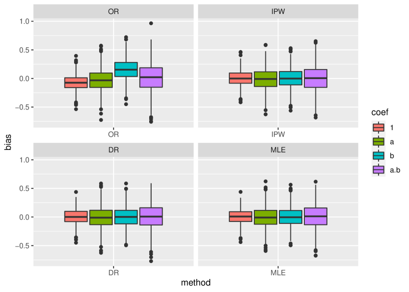
Figure 3: Boxplots of the bias for each coefficient by four methods: outcome regression (OR), inverse probability weighting (IPW), doubly robust estimation (DR), and maximum likelihood estimation (MLE).

5.2 Data Analysis

To illustrate our method, we apply the maximum likelihood fitting procedure to data from the IDEFICS study (Ahrens et al., 2011). The subset of data we use consists of measurements of 531 German children aged between 2 and 9, including their sex, physical activity, screen time, parental education, a ‘vegetable score’, fibre intake, and a polygenic risk score (PRS) for BMI. The study also records the child’s BMI and their parents’ BMIs. Preliminary analyses suggest that increased fibre intake can reduce BMI, especially for those children who have a strong genetic predisposition for obesity (Hüls et al., 2021). Our aim is to study the effect modification of PRS on the relationship between fibre intake and actual BMI, whilst adjusting for confounding due to other covariates.

We replicate the setting in Nöhren (2021), which considers how the causal effect of a dichotomized indicator of fibre intake ($X$) on age and sex standardized BMI ($Y$, a z-score) interacts with the dichotomized polygenic risk score ($C$); like Nöhren we also use a marginal structural model:

$$\mathbb{E}[Y\,|\,C=c;\mathit{do}(X=x)]=\beta_{0}+\beta_{1}x+\beta_{2}c+\beta_{3}cx.$$

We assume that all other variables are causally prior to $X$, so that $\mathbb{E}[Y\,|\,C=c;\mathit{do}(X=x)]$ is our causal distribution of interest, where $\bm{Z}$ consists of other confounders; these include sex, age, physical activity, screen time, vegetable score and a dichotomized version of parental education level.

We choose an ordinary Gaussian linear model for the MSM, and also the other models used for variables in $\bm{Z}$. The copula was also Gaussian. Note that in order to accommodate sex and parental education as binary variables it was necessary to integrate over the copula, effectively making it a probit model (see also Example 2.6).

The relevant coefficients from the model fit are shown in Table 2. Under our modelling assumptions, these results do not suggest that increased fibre intake reduces BMI and thus we cannot confirm previous results obtained on a larger dataset of 2,688 children from seven countries (Nöhren, 2021); the estimates from that study are within our (rather wide) confidence intervals, though. Furthermore, the analysis of Nöhren for the marginal structural model using inverse probability weighting on only the German data yields slightly different parameter estimates, and larger standard errors (see Appendix E for details). This illustrates—in a practical analysis—the differences between, on the one hand, modelling the $C$-$Y$-$\bm{Z}$ association directly or, on the other hand, modelling the propensity score for the inverse probability weights.

param.	coefficient	est.	s.e.	95% conf. int.
$\beta_{1}$	fibre	0.049	0.092	$-$0.132	0.230
$\beta_{2}$	PRS	0.374	0.198	$-$0.015	0.762
$\beta_{3}$	PRS:fibre	0.011	0.359	$-$0.693	0.715

Table 2: Table giving estimated coefficients in the marginal structural model for effect modification of the PRS on BMI by fibre intake.

6 Survival Models

Another application of the frugal parameterization is to causal longitudinal models, and in particular to survival models. Note that with sequences of treatment variables, the sequential versions of identifying assumptions must be met (cf. Remark 1.5) known as sequential conditional exchangeability; we continue to take these as given in Sections 6 and 7.

The following corollary of Theorem 3.1 allows us to ‘build up’ a frugal parameterization of the joint distribution using several different cognate quantities. Given a collection of variables $Y_{1},\ldots,Y_{d}$ under some natural ordering (typically a temporal ordering), let $[i-1]=\{1,\ldots,i-1\}$ denote the predecessors of each $i=1,\ldots,d$.

Corollary 6.1.

Let $Y_{1},\ldots,Y_{d}$ have joint density $p$, and let $X_{i}:=Y_{A_{i}}=\{Y_{j}:j\in A_{i}\}$ for some $A_{i}\subseteq[i-1]$. Also let $p_{Y_{i}|X_{i}}^{*}(y_{i}\,|\,x_{i})$ be defined by applying (3) with $Z_{i}:=Y_{L_{i}}$ where $L_{i}:=[i-1]\setminus A_{i}$.

Then there is a smooth and regular parameterization of the joint distribution, which can be chosen to be variation independent, containing each $p_{Y_{i}|X_{i}}^{*}(y_{i}\,|\,x_{i})$.

Proof.

We proceed by induction. For $i=1$ we just have a smooth and regular parameterization of $p_{Y_{1}}(y_{1})$. For a general $i$, assume we have a smooth parameterization of the joint density for $Y_{1},\ldots,Y_{i-1}$ and of $p_{Y_{i}|X_{i}}^{*}(y_{i}\,|\,x_{i})$. Then using some appropriate $\phi_{Y_{i}Z_{i}\mid X_{i}}^{*}$ to make up a frugal parameterization (and A1 if required), by Theorem 3.1 we obtain a smooth and regular parameterization of the joint density for $Y_{1},\ldots,Y_{i}$, and—if A1 holds—the quantities used are all variation independent of one another. ∎

We refer to this approach as a recursive or nested frugal parameterization, because in each case ‘the past’ (i.e. $p_{{ZX}}$) is itself parameterized in a frugal manner.

Example 6.2.

Young and Tchetgen Tchetgen (2014) consider survival models with time-varying covariates and treatments. Let $Y_{t}=0$ be an indicator of survival up to time $t$ (with $Y_{t}=1$ indicating failure). Let $L_{t},A_{t}$ be respectively covariates and treatment at time $t=0,\ldots,T$. Young and Tchetgen Tchetgen model the quantities

$$P(Y_{t}=0\,|\,Y_{t-1}=0;\mathit{do}(a_{1},\ldots,a_{t-1})), t=1,\ldots,T;$$

i.e. probability of survival to the next time point given treatment history and survival so far. Under their assumptions these quantities are identifiable via the g-formula as

$$p(y_{t}\,|\,y_{t-1};\mathit{do}(\overline{a}_{t-1}))=\sum_{\overline{\ell}_{t}}p(y_{t}\,|\,y_{t-1},\overline{a}_{t-1},\overline{\ell}_{t})\prod_{s=1}^{t}p(\ell_{s}\,|\,\overline{a}_{s-1},\overline{\ell}_{s-1});$$ (7)

note that we omit some subscripts on densities for brevity. Corollary 6.1 tells us that, setting $X_{t}=\overline{A}_{t}$ and $Z_{t}=\overline{L}_{t}$, a parameterization exists of the joint distribution that uses these quantities for each $t=1,\ldots,T$. Given the distribution of $p(\overline{a}_{t-1},\overline{\ell}_{t-1},\overline{y}_{t-1})$, the quantities

$$p(y_{t}\,|\,y_{t-1};\mathit{do}(\overline{a}_{t-1})) \phi^{*}_{Y_{t}\overline{L}_{t-1}|\overline{A}_{t-1}\overline{Y}_{t-1}}(y_{t},\overline{\ell}_{t-1}\,|\,\overline{a}_{t-1},\overline{y}_{t-1})$$

may be used to recover $p(\overline{a}_{t-1},\overline{\ell}_{t-1},\overline{y}_{t})$.

Young and Tchetgen Tchetgen (2014) note that simulation from this model is difficult for certain parametric choices, because some parameters from the joint model and the marginal model are tied together in complicated ways. They derive results that allow them to compute particular causal parameters as functions of the joint distribution, and hence to evaluate the performance of simulation methods exactly. Our approach overcomes this problem by allowing causal quantities of interest to be specified explicitly, and then have the rest of the distribution constructed around them.

The model is parameterized so that failure is a rare outcome, which allows approximation of the expit function by an exponential function. The parameters of interest are then those of the Cox Marginal Structural Model:

$$\frac{p_{Y_{t}|\overline{A}_{t}Y_{t-1}}^{*}(1\,|\,\mathit{do}(\overline{a}_{t}),Y_{t-1}=0)}{p_{Y_{t}|\overline{A}_{t}Y_{t-1}}^{*}(1\,|\,\mathit{do}(\overline{0}_{t}),Y_{t-1}=0)} =e^{\gamma(t,\overline{a}_{t})}=\exp\left(\psi_{0}a_{t}+\psi_{1}a_{t-1}+\psi_{01}a_{t}a_{t-1}\right),$$

which, as we see above, the authors assume to depend only upon the previous two treatments. These parameters $\psi$ are estimated by fitting an inverse weighted GLM to the data.

The authors also state that: ‘[we] therefore, may be limited to simulation scenarios with the proposed algorithm to particularly unrealistic settings if we wish simultaneously to generate data under the null.’ Our results demonstrate that if one uses our algorithms this is not the case. The null in this example corresponds to $\psi_{0}=\psi_{1}=\psi_{01}=0$; since the model is discrete we are free to choose arbitrary regression models for the treatment on the observed past, for the covariates on their past values and treatments (and even unobserved quantities), and any arbitrary dependence structure between survival and the covariates, conditional on all previous treatments and covariates. This will allow us to simulate from any distribution under which treatment has no (marginal) causal effect upon survival. In Appendix F we perform some simulations on this model.

7 Structural Nested Model Parameterizations

Not all causal parameterizations involve modelling the entire conditional distribution for every level of the conditioning variable; i.e. quantities of the form $p_{{Y|X}}^{*}(y\,|\,x)$ for every value of $x\in\mathcal{X}$. The structural nested models of Robins and Tsiatis (1991) are an example of this. These allow for interactions between time-varying covariates and time-varying treatments, but they are always marginal over future covariates; this makes them considerably more flexible than marginal structural models, because they allow for dependence in treatment decisions on all observed data. We again continue to make the necessary assumptions for identifiability; see Robins and Tsiatis (1991) for more detail.

Example 7.1 (Structural Nested Models).

Suppose we have a sequence of binary treatments $A_{1},\ldots,A_{T}$ and time-varying covariates $L_{1},\ldots,L_{T}$, together with an outcome $Y$. Let $\overline{L}_{t}\equiv(L_{1},\ldots,L_{t})$ and $\underline{L}_{t}\equiv(L_{t},\ldots,L_{T})$, and similarly for $\overline{A}_{t}$, $\underline{A}_{t}$. The structural nested model (Robins and Tsiatis, 1991) involves contrasts between $a_{t}=0,1$ of the form:

$$p_{Y|\overline{L}_{t}\overline{A}_{T}}(y\,|\,\overline{\ell}_{t},\overline{a}_{t-1};\mathit{do}(a_{t},\underline{a}_{t+1}=0)), \forall\,\overline{\ell}_{t},\overline{a}_{t-1},t=0,\ldots,T.$$

The parameterization divides the effect of the treatments into pieces corresponding to ‘blips’ of effect at each time point: that is, at each time $t$, we consider the effect of receiving treatment at that time but no further treatment, versus never receiving any treatment from time $t$ onwards. The contrast may be in the form of a risk difference, risk ratio or other suitable quantity.

We represent such a generic contrast by introducing a tilde above the variable being contrasted; in the above example we would write:

$$p_{Y|\overline{L}_{t}\overline{A}_{T}}(y\,|\,\overline{\ell}_{t},\overline{a}_{t-1};\mathit{do}(\widetilde{a}_{t},\underline{a}_{t+1}=0)), \forall\,\overline{\ell}_{t},\overline{a}_{t-1},t=0,\ldots,T.$$ (8)

See the more formal Definition 7.2 below.

We define two additional kinds of parameter to generalize these ideas.

Definition 7.2.

Let $q_{{Y|XZ}}(y\,|\,x,z)$ be a conditional distribution. We denote by $q_{Y|XZ}(y\,|\,x^{0},z)$ a baseline parameter, which can smoothly recover the relevant conditional distribution at a particular baseline value $X=x^{0}$.

We will denote by $q_{Y|XZ}(y\,|\,\widetilde{x},z)$ a contrast parameter (over $X$). We define the pair of baseline and contrast parameters to be a full parameterization if, when we combine them, we can smoothly recover all of $q_{Y|XZ}(y\,|\,x,z)$.

In the appendix we give Lemma B.1, showing we can use risk differences, risk ratios or odds ratios as contrast parameters, if $p>0$ and each $X_{t}$ is binary. Examples of a set of baseline parameters might be $(\beta_{0},\beta_{z},\sigma^{2})$ for some regression model $y=\beta_{0}+\beta_{x}x+\beta_{z}z+\varepsilon$, where $\operatorname{Var}\varepsilon=\sigma^{2}$; the natural contrast parameter would then be $\beta_{x}$. Alternatively it might be the density $p_{{Y|XZ}}(y\,|\,x^{0},z)$, $y\in\mathcal{Y},z\in Z$, for some value $x^{0}\in\mathcal{X}$; the contrast parameter could then be a risk ratio:

$$p_{{Y|XZ}}(y\,|\,\tilde{x},z)\equiv\frac{p_{{Y|XZ}}(y\,|\,x,z)}{p_{{Y|XZ}}(y\,|\,x^{0},z)}\quad\text{for all }x\in\mathcal{X},y\in\mathcal{Y},z\in\mathcal{Z}.$$

7.1 Iterated Frugal Parameterization

How can we use the frugal parameterization to obtain the structural nested model? We now introduce the iterated frugal parameterization to allow us to do just that.

Consider a sequence of random variables $L_{1},A_{1},L_{2},\ldots,L_{T},A_{T}$ and an outcome of interest $Y$. Assume also that there is a natural ‘baseline’ treatment level $A_{i}=a_{i}^{0}$. Then the iterated frugal parameterization consists of a parameterization of ‘the past’ (i.e. $p_{{ZX}}$), of $p^{*}_{Y|L_{1}\overline{A}_{T}}(y\,|\,\ell_{1},\overline{a}^{0}_{T})$, and the following quantities:

$$\left.\begin{array}[]{l}p^{*}_{Y|\overline{L}_{t}\overline{A}_{T}}(y\,|\,\overline{\ell}_{t},\overline{a}_{t-1},\widetilde{a}_{t},\underline{a}^{0}_{t+1})\\[6.0pt] \phi_{Y\!L_{t+1}|\overline{L}_{t}\overline{A}_{t}}^{*}(y,\ell_{t+1}\,|\,\overline{\ell}_{t},\overline{a}_{t})\end{array}\right\}\qquad\begin{array}[]{l}\forall y,\overline{\ell}_{T},\overline{a}_{T}\\ t=1,\ldots,T,\end{array}$$

where the parameters can be used to obtain $p^{*}_{Y|\overline{L}_{t}\overline{A}_{T}}(y\,|\,\overline{\ell}_{t},\overline{a}_{t-1},a^{0}_{t},\underline{a}^{0}_{t+1})$ such that combined with $p^{*}_{Y|\overline{L}_{t}\overline{A}_{T}}(y\,|\,\overline{\ell}_{t},\overline{a}_{t-1},\widetilde{a}_{t},\underline{a}^{0}_{t+1})$ we obtain a ‘full’ parameterization (for $p^{*}_{Y|\overline{L}_{t}\overline{A}_{T}}(y\,|\,\overline{\ell}_{t},\overline{a}_{t},\underline{a}^{0}_{t+1})$). Note that if we consider the contrast parameter to be all the possible values other than the baseline value, then each state of $\overline{a}_{T}$ will appear on the right-hand side of a quantity $p^{*}_{Y|\overline{L}_{t}\overline{A}_{T}}$ exactly once.

7.2 The Structural Nested Model

How can we use a parameterization that incorporates all the quantities (8)? Based on the temporal ordering, and given $p_{Y|\overline{L}_{t}\overline{A}_{T}}(y\,|\,\overline{\ell}_{t},\overline{a}_{t-1};\mathit{do}(a_{t},\underline{a}_{t+1}=0))$ and

$$p_{L_{t+1}|\overline{L}_{t}\overline{A}_{T}}(\ell_{t+1}\,|\,\overline{\ell}_{t},\overline{a}_{t-1};\mathit{do}(a_{t},\underline{a}_{t+1}=0))=p_{L_{t+1}|\overline{L}_{t}\overline{A}_{t}}(\ell_{t+1}\,|\,\overline{\ell}_{t},\overline{a}_{t}),$$

we need $\phi^{*}_{Y\!L_{t+1}|\overline{L}_{t}\overline{A}_{t}}(y,\ell_{t+1}\,|\,\overline{\ell}_{t},\overline{a}_{t})$ to recover the joint $p_{Y\!L_{t+1}|\overline{L}_{t}\overline{A}_{T}}(y,\ell_{t+1}\,|\,\overline{\ell}_{t},\overline{a}_{t};\mathit{do}(\underline{a}_{t+1}=0))$. Then notice

$$p(y,\overline{\ell}_{T}\,|\,\overline{a}_{t};\mathit{do}(\underline{a}_{t+1}))=p(y,\overline{\ell}_{T}\,|\,\overline{a}_{t+1};\mathit{do}(\underline{a}_{t+2}))\cdot\frac{p(a_{t+1}\,|\,\overline{a}_{t})}{p(a_{t+1}\,|\,\overline{\ell}_{t},\overline{a}_{t})},$$

so we can ‘change worlds’ and obtain probabilities with the same settings from a reweighting that is identifiable from the previous variables. The following proposition gives the general result, proved and illustrated by examples in Appendix B.

Proposition 7.3.

We can parameterize $p_{\overline{L}_{T}\overline{A}_{T}Y}(\overline{\ell}_{T},\overline{a}_{T},y)$ using smooth and regular parameterizations for $p^{*}_{Y|L_{1}\overline{A}_{T}}(y\,|\,\ell_{1},\overline{a}^{0}_{T})$ and

$$\left.\begin{array}[]{l}p_{L_{t}A_{t}|\overline{L}_{t-1}\overline{A}_{t-1}}(\ell_{t},a_{t}\,|\,\overline{\ell}_{t-1},\overline{a}_{t-1})\\[6.0pt] p^{*}_{Y|\overline{L}_{t}\overline{A}_{T}}(y\,|\,\overline{\ell}_{t},\overline{a}_{t-1},\widetilde{a}_{t},\underline{a}^{0}_{t+1})\\[6.0pt] \phi_{Y\!L_{t+1}|\overline{L}_{t}\overline{A}_{t}}^{*}(y,\ell_{t+1}\,|\,\overline{\ell}_{t},\overline{a}_{t})\end{array}\right\}\qquad\begin{array}[]{l}\forall y,\overline{\ell}_{T},\overline{a}_{T}\\ t=1,\ldots,T,\end{array}$$

where each $p^{*}_{Y|\overline{L}_{t}\overline{A}_{T}}$ is cognate for the particular baseline $\underline{a}^{0}_{t+1}$. In particular, our parameterization can include ‘blips’ such as those in (8). If either the contrast parameter is the odds ratio, or the risk ratio and the outcome is positive and unbounded, then these pieces are also variation independent.

The proof for the special case of binary treatment variables is given in Appendix B. With this general formulation we do not require $p^{*}_{Y|\overline{L}_{t}\overline{A}_{T}}$ to be of the same form for each $t=1,\ldots,T$; this flexibility may be useful for many settings. However, we do need the baseline level $\underline{a}_{t+1}^{0}$ to be consistent over all $t$, since otherwise the inductive argument we use will not work. Note also that $\phi^{*}_{Y\!L_{T+1}|\overline{L}_{T}\overline{A}_{T}}$ is trivial, since $L_{T+1}$ is assumed constant.

Two numerical examples are given as RB.1 and B.2 in Appendix B.

Remark 7.4.

The History-Adjusted Marginal Structural Models (HAMSMs) introduced by van der Laan et al. (2005) model (the mean of) the distributions

$$p_{Y|\overline{L}_{t}\overline{A}_{T}}(y\,|\,\overline{a}_{t-1},\overline{\ell}_{t};\mathit{do}(\underline{a}_{t})),\qquad t=1,\ldots,T.$$

This is similar to the form of a structural nested mean model, but in this case we attempt to model all future treatment regimes simultaneously, not just at a baseline $\underline{a}_{t}=0$. This effectively requires us to model the association between $Y$ and each $A_{t}$ multiple times in different margins, and hence we will be using parameters that are redundant; it therefore does not fall within our frugal framework. This was pointed out by Robins et al. (2007), who showed that it is a non-congenial parameterization, and may lead to incompatible distributions.

8 Discussion and Conclusion

As we have demonstrated, the principle of a frugal parameterization is widely applicable and useful in many marginal modelling contexts, especially causal models. We begin this discussion by briefly considering three more key settings for causal models: sensitivity analysis, instrumental variable (IV) analysis and mediation analysis.

In sensitivity analysis, a key challenge is to construct an augmented model that is compatible with the original model in the sense that it shares a marginal distribution over the observed variables, but can be tweaked to introduce various levels of unobserved confounding. This is clearly possible within our framework; considering Example RC in Appendix C, we can set the correlations involving $U$ to zero, and then increase them to test the dependence of our conclusions to the presence of an unobserved confounder.

In an IV analysis, the instrument is used as an imperfect replacement for randomization when the actual treatment $X$ is affected by unobserved confounding. To formulate a generative IV model we typically want to combine a desired parameterization for $p_{{Y|X}}^{*}(y\,|\,\mathit{do}(x))$ with a model that includes the IV and the confounder $U$. The difficulty, here, is due to the particular properties of an IV which require the joint model to satisfy certain conditional independence properties while being compatible with the marginal causal model. This is especially problematic for non-collapsible cases, for instance for logistic structural mean models (Robins and Rotnitzky, 2004; Vansteelandt et al., 2011; Clarke and Windmeijer, 2012) or structural Cox models (Martinussen et al., 2017). As outlined in Appendix G, we believe that our approach based on the frugal parameterization can also be helpful in these situations, but we leave details for future work.

In contrast, causal mediation analysis is an example where models contain singularities and therefore our approach cannot be applied. Decomposing the effect of a treatment $A$ on outcome $Y$ into the indirect effect via mediator $M$, and the remaining direct effect, is conceptually the same as splitting $A$ into two separate nodes $A,A^{\prime}$, where observationally we always have $A=A^{\prime}$; mediation questions may then be considered as asking what would happen if $A\neq A^{\prime}$ (Robins and Richardson, 2010). The quantities of interest are therefore generally functions of $p_{Y|AA^{\prime}}(y\,|\,\mathit{do}(a,a^{\prime}))$, but where at the same time $Y\mathchoice{\mathrel{\hbox to0.0pt{$\displaystyle\perp$\hss}\mkern 2.0mu{\displaystyle\perp}}}{\mathrel{\hbox to0.0pt{$\textstyle\perp$\hss}\mkern 2.0mu{\textstyle\perp}}}{\mathrel{\hbox to0.0pt{$\scriptstyle\perp$\hss}\mkern 2.0mu{\scriptstyle\perp}}}{\mathrel{\hbox to0.0pt{$\scriptscriptstyle\perp$\hss}\mkern 2.0mu{\scriptscriptstyle\perp}}}A^{\prime}\mid A,M$ holds in the full model where the two treatments are potentially different (Didelez, 2019). Because this independence requires us to model the $Y$-$A^{\prime}$ association within the joint distribution, not within the $(Y,A,A^{\prime})$-margin, the only parameters that we are free to specify are then those of the distribution of $Y$ given each level of $A$ (i.e. the strength of the direct effect); this is explicitly possible in the discrete case using results in Evans (2015). In other cases, attempts to specify both $p^{*}_{Y|AA^{\prime}}$ and $p^{*}_{Y|AA^{\prime}\!M}$ separately may lead to models which are not compatible; for example, the equations (4) and (5) of Loeys et al. (2013) do not generally give a valid model because the logit function is not closed under marginalization. Lange et al. (2012) avoid the problem of explicitly modelling the joint distribution by using marginal structural models instead, though their approach does not allow for simulation from the resulting model.

Another example of nonsmoothness comes from quantities such as $\mathbb{E}_{\theta}[Y\,|\,\mathit{do}(x)]-\mathbb{E}_{\theta}[Y\,|\,x]$, or some other contrast between these two distributions. This leads to a parameterization which is degenerate, in the sense that its derivative (or nonparametric equivalent) is zero in some directions when the two distributions are the same.

While such nonsmooth models still remain a challenge, we are certain that marginal models based on a frugal parameterization have many further useful applications and extensions worth exploring in future work. For instance, classes of distribution that are closed under marginalization and conditioning, such as MTP₂ distributions (Karlin and Rinott, 1980), will naturally combine with our approach. On the technical side, the proposed rejection sampling method can be inefficient, and it would be desirable to improve this by using more advanced methods, along the lines of those suggested by Jacob et al. (2020).

As we noted in Section 1.2, we can see two opposing or complementary trends in causal modelling: many approaches are based on specifying structural causal models that implicitly or explicitly condition on the entire past, and do not consider marginal objects such as $p_{{Y|X}}(y\,|\,\mathit{do}(x))$. In contrast, our approach is found in the books by Pearl (2009, Chapter 3), Imbens and Rubin (2015) and Hernán and Robins (2020), which all consider marginal causal quantities to be fundamental. Beyond frugal parameterizations, we believe that thinking about causal models as a form of marginal model, for which there is an older and richer literature, may lead to many more advances in the field.

Acknowledgements

We are grateful to Bohao Yao for some early simulations, as well as to Thomas Richardson, James Robins, Ilya Shpitser, the Associate Editor and four anonymous reviewers for their insights and suggestions. We would also like to thank Qingyuan Zhao for reading a late draft and providing very insightful comments and corrections, including the idea about a sensitivity analysis. Part of a revision of the manuscript was undertaken while both authors were Visiting Scientists at the Simons Institute, Berkeley.

Section 5.2 was done as part of the IDEFICS Study. The data used in this article cannot be shared publicly due to confidentiality policies agreed with the families participating in the study. We gratefully acknowledge the financial support of the European Commission within the Sixth RTD Framework Programme Contract No. 016181. The authors have no conflicts of interest to declare.

Appendix A Smoothness, Regularity and Singularity

The first few definitions in this section are adapted from Newey (1990) and Chapter 5 of van der Vaart (1998). Suppose that we have have a parametric family of distributions $\mathcal{M}=\{p_{\theta}:\theta\in\Theta\subseteq\mathbb{R}^{d}\}$, indexed by a parameter $\theta$.

Definition A.1.

We say that the model $\mathcal{M}$ is differentiable in quadratic mean if there exists a function $\dot{\ell}(\theta_{0})$ such that as $\theta\to\theta_{0}$,

$$\int\left[\sqrt{p_{\theta}}-\sqrt{p_{\theta_{0}}}-\frac{1}{2}(\theta-\theta_{0})^{T}\dot{\ell}(\theta_{0})\sqrt{p_{\theta_{0}}}\right]\,d\mu=o(\|\theta-\theta_{0}\|^{2}).$$

If a model is differentiable in quadratic mean we say that the parameterization induced by $\theta$ is smooth. Now, for almost all statistical models of interest, $\dot{\ell}$ is of course the score function, that is

$$\dot{\ell}(\theta)=\frac{\partial}{\partial\theta}\log p_{\theta}.$$

In this case, if the Fisher information matrix

$$I(\theta)=\mathbb{E}\dot{\ell}(\theta)\dot{\ell}(\theta)^{T}$$

is non-singular, then we also say that the map defined by $\theta$ is a regular parameterization.

We also have related but separate terminology for submodels, which we adapt from Drton (2009).

Definition A.2.

Given a submodel of $\mathcal{M}$, say $\mathcal{M}^{\prime}\subseteq\mathcal{M}$, we say that $\mathcal{M}^{\prime}$ is nonsingular if the induced subset of $\Theta$ is everywhere locally Euclidean and of constant dimension. Otherwise the model has points of singularity or singularities.

An example of a model with singularities would be the union of the axes $\{(\theta_{1},\theta_{2}):\theta_{1}\theta_{2}=0\}$, because this model is not locally Euclidean at $\theta_{1}=\theta_{2}=0$.

Appendix B Proof of Proposition 7.3

We extend the notion of a risk difference, risk ratio or odds ratio to a general outcome variable (but still binary treatment) by writing

$$\operatorname{RD} :=p_{{Y|ZX}}(y\,|\,z,x=1)-p_{{Y|ZX}}(y\,|\,z,x=0)$$

$$\operatorname{RR} :=\frac{p_{{Y|ZX}}(y\,|\,z,x=1)}{p_{{Y|ZX}}(y\,|\,z,x=0)}$$

$$\operatorname{OR} :=\frac{p_{{Y|ZX}}(y\,|\,z,x=1)\cdot p_{{Y|ZX}}(y^{0}\,|\,z,x=0)}{p_{{Y|ZX}}(y^{0}\,|\,z,x=1)\cdot p_{{Y|ZX}}(y\,|\,z,x=0)}$$

for some arbitrary baseline value $y^{0}$. This latter definition is a special case of the one used by Chen (2007).

Lemma B.1.

Suppose $p>0$, and that $X$ is binary. Given $p_{{ZX}}(z,x)$, $p_{Y|Z}(y\,|\,z)$ and $p_{{Y|ZX}}(y\,|\,z,\widetilde{x})$, where $\widetilde{x}$ is contrasted using a risk difference, risk ratio or an odds ratio, we can smoothly recover $p_{{Y|ZX}}(y\,|\,z,x)$. In addition, if we use the risk ratio and the range of $Y>0$ is unbounded, or we use the odds ratio these three pieces will be variation independent.

Proof.

For a risk difference or ratio, it is clear that if $p_{{ZX}}(z,x)$ and $p_{Y|Z}(y\,|\,z)$ are fixed, then

$$\theta_{z} =p_{{Y|ZX}}(y\,|\,z,x=1)-p_{{Y|ZX}}(y\,|\,z,x=0)$$

$$\theta^{\prime}_{z} =\frac{p_{{Y|ZX}}(y\,|\,z,x=1)}{p_{{Y|ZX}}(y\,|\,z,x=0)}$$

each give a regular representation of $p_{{Y|ZX}}(y\,|\,z,x)$ when combined with

$$p_{Y|Z}(y\,|\,z)=\sum_{x=0}^{1}p_{X|Z}(x\,|\,z)p_{{Y|ZX}}(y\,|\,z,x).$$

For the odds ratio we refer to Chen (2007) for details. The variation independence of the odds ratio from its margins is well known (e.g. Rüschendorf, 1995). If $Y$ is unbounded and $p_{{Y|ZX}}(y\,|\,z,\widetilde{x})$ is the risk-ratio, then it is clear that we can modify it in any way and still obtain a valid joint distribution. ∎

Proof of Proposition 7.3.

We consider the special case in which each $A_{t}$ is binary, and proceed by induction on $T$. Note that we can combine all the conditionals $p_{L_{t}A_{t}|\overline{A}_{t-1}\overline{L}_{t-1}}$ to obtain the joint distribution $p_{\overline{L}_{T}\overline{A}_{T}}$. Now, by a simple adaptation of Theorem 3.1, we start with

$$p^{*}_{Y|L_{1}\overline{A}_{T}}(y\,|\,\ell_{1},\underline{a}_{1}^{0})\qquad p^{*}_{Y|L_{1}\overline{A}_{T}}(y\,|\,\ell_{1},\widetilde{a}_{1},\underline{a}_{2}^{0})\qquad\phi^{*}_{Y\!L_{2}|L_{1}A_{1}}(y,\ell_{2}\,|\,\ell_{1},a_{1}),$$

from which we can recover $p^{*}_{Y|L_{1}\overline{A}_{T}}(y\,|\,\ell_{1},a_{1},\underline{a}_{2}^{0})$ by Lemma B.1. We can then combine with $p_{L_{2}|L_{1}A_{1}}$ and $\phi^{*}_{Y\!L_{2}|L_{1}A_{1}}$ to obtain $p^{*}_{Y\!L_{2}|L_{1}\overline{A}_{T}}(y,\ell_{2}\,|\,\ell_{1},a_{1},\underline{a}_{2}^{0})$, and consequently (by reweighting) $p_{Y\!L_{2}|L_{1}\overline{A}_{T}}(y,\ell_{2}\,|\,\ell_{1},a_{1},\underline{a}_{2}^{0})$.

Now, assume for induction that we can recover $p_{Y|\overline{L}_{t}\overline{A}_{T}}(y\,|\,\overline{\ell}_{t},\overline{a}_{t-1},\underline{a}_{t}^{0})$; we have shown this for $t=2$. We can reweight with some function of $p_{\overline{L}_{T}\overline{A}_{T}}$ to obtain $p^{*}_{Y|\overline{L}_{t}\overline{A}_{T}}(y\,|\,\overline{\ell}_{t},\overline{a}_{t-1},\underline{a}_{t}^{0})$, and then combining with $p^{*}_{Y|\overline{L}_{t}\overline{A}_{T}}(y\,|\,\overline{\ell}_{t},\overline{a}_{t-1},\widetilde{a}_{t},\underline{a}^{0}_{t+1})$ and again using Lemma B.1 we obtain $p^{*}_{Y|\overline{L}_{t}\overline{A}_{T}}(y\,|\,\overline{\ell}_{t},\overline{a}_{t},\underline{a}_{t+1}^{0})$. Then, we can again use $\phi^{*}_{Y\!L_{t+1}|\overline{L}_{t}\overline{A}_{t}}$ together with $p^{*}_{Y|\overline{L}_{t}\overline{A}_{T}}$ and $p^{*}_{L_{t+1}|\overline{L}_{t}\overline{A}_{T}}$ (for $\underline{A}_{t+1}=\underline{a}^{0}_{t+1}$) to obtain $p^{*}_{Y\!L_{t+1}|\overline{L}_{t}\overline{A}_{t}}$. Reweighting again yields an expression for $p_{Y\!L_{t+1}|\overline{L}_{t}\overline{A}_{T}}$ when $\underline{A}_{t+1}=\underline{a}^{0}_{t+1}$, and hence $p_{Y|\overline{L}_{t+1}\overline{A}_{T}}(y\,|\,\overline{\ell}_{t+1},\overline{a}_{t},\underline{a}_{t+1}^{0})$.

Hence, by induction, we can obtain $p_{Y|\overline{L}_{T}\overline{A}_{T}}$, and consequently $p_{\overline{L}_{T}\overline{A}_{T}Y}$.

The results on variation independence follow directly from the implications in Lemma B.1. ∎

Example R6. Consider again the model in Figure 2; in this case, we have $A_{1}=A$ and $A_{2}=B$, with $L_{2}=L$ and $L_{1}$ being null. A structural nested mean model would include

$$p_{{Y|AB}}(y\,|\,\mathit{do}(a=b=0)) p_{{Y|AB}}(y\,|\,\mathit{do}(a=1,b=0))$$

and $$p_{{Y|ALB}}(y\,|\,a,\ell;\mathit{do}(\tilde{b})).$$

In order to complete the parameterization we also need $p_{{ALB}}$ and $\phi^{*}_{Y\!L|A}$; the latter of these could be the conditional odds ratio in the discrete case, for example. The advantage of this representation of an SNM is that it makes absolutely clear which (groups of) parameters are free to be varied. Indeed, like the previous examples this ‘model’ is such that any distribution over $A,L,B,Y$ (or more generally $\overline{A}_{T},\overline{L}_{T},Y$) can be represented using this parameterization.

We demonstrate this by constructing a distribution for a structural nested mean model over this graph. We take all variables to be binary, and let the blips be in the form of risk differences:

$$p_{{Y|AB}}(1\,|\,\mathit{do}(a=b=0)) =0.2$$

$$p_{{Y|AB}}(1\,|\,\mathit{do}(a=1,b=0))-p_{{Y|AB}}(1\,|\,\mathit{do}(a=b=0)) =0.1$$

$$p_{{Y|ALB}}(1\,|\,a,\ell;\mathit{do}(b=1))-p_{{Y|ALB}}(1\,|\,a,\ell;\mathit{do}(b=0)) =0.1a+0.05\ell.$$

Suppose also that $p_{A}(1)=0.3$, and

$$p_{L|A}(1\,|\,a) =0.4-0.1a$$

$$p_{B|AL}(1\,|\,a,\ell) =0.2+0.3a+0.3\ell$$

$$\log\phi_{Y\!L|A}(1,1\,|\,a) =0.1+0.1a,$$

where $\phi_{Y\!L|A}$ is the conditional odds ratio. The resulting conditional probabilities $p_{{Y|ALB}}(1\,|\,a,\ell,b)$ are given in Table 3.

$a$	$\ell$	$b$	$p_{{Y|ALB}}(1\,|\,a,\ell,b)$
0	0	0	0.194
1	0	0	0.287
0	1	0	0.210
1	1	0	0.330
0	0	1	0.194
1	0	1	0.387
0	1	1	0.260
1	1	1	0.480

Table 3: Table giving probability of survival from the SNMM in Example RB.1.

Example B.2.

This is an expansion of Example RB.1 in the notation of Section 7: hence $(A,B)$ becomes $(A_{1},A_{2})$, and $L$ becomes $L_{2}$. We also add in a ‘static’ covariate $L_{1}$ that is causally prior to all other variables. Suppose that $T=2$, all variables are binary, and let the blips be in the form of risk differences:

$$p_{Y|L_{1}\overline{A}_{2}}(1\,|\,\ell_{1};\mathit{do}(a_{1}=a_{2}=0)) =0.2$$

$$p_{Y|L_{1}\overline{A}_{2}}(1\,|\,\ell_{1};\mathit{do}(a_{1}=1,a_{2}=0))-p_{Y|L_{1}\overline{A}_{2}}(1\,|\,\ell_{1};\mathit{do}(a_{1}=a_{2}=0)) =0.1+0.1\ell_{1}$$

$$p_{Y|\overline{L}_{2}\overline{A}_{2}}(1\,|\,\ell_{1},a_{1},\ell_{2};\mathit{do}(a_{2}=1))-p_{Y|\overline{L}_{2}\overline{A}_{2}}(1\,|\,\ell_{1},a_{1},\ell_{2};\mathit{do}(a_{2}=0)) =0.05\ell_{1}+0.05\ell_{2}+0.1a_{1}.$$

Suppose also that $p_{L_{1}}(1)=0.5$ and $p_{A_{1}|L_{1}}(1\,|\,\ell_{1})=0.3+0.3\ell_{1}$, and

$$p_{L_{2}|L_{1}A_{1}}(1\,|\,\ell_{1},a_{1}) =0.4+0.3\ell_{1}-0.1a_{1}-0.2\ell_{1}a_{1}$$

$$p_{A_{2}|\overline{L}_{2}A_{1}}(1\,|\,\ell_{1},\ell_{2},a_{1}) =0.2+0.3a_{1}+0.3\ell_{2}$$

$$\log\phi_{Y\!L_{2}|L_{1}\!A_{1}}(1,1\,|\,\ell_{1},a_{1}) =0.1+0.1\mathbb{I}_{\{a_{1}=\ell_{1}\}},$$

where $\phi_{Y\!L_{2}|L_{1}\!A_{1}}$ is the conditional odds ratio. The resulting conditional probabilities $p_{Y|\overline{L}_{2}\overline{A}_{2}}(1\,|\,\overline{\ell}_{2},\overline{a}_{2})$ are given in Table 4.

$\ell_{1}$	$\ell_{2}$	$a_{1}$	$a_{2}$	$p_{Y|\overline{L}_{2}\overline{A}_{2}}(1\,|\,\overline{\ell}_{2},\overline{a}_{2})$
0	0	0	0	0.187
1	0	0	0	0.189
0	1	0	0	0.219
1	1	0	0	0.205
0	0	1	0	0.294
1	0	1	0	0.381
0	1	1	0	0.315
1	1	1	0	0.429
0	0	0	1	0.187
1	0	0	1	0.239
0	1	0	1	0.269
1	1	0	1	0.305
0	0	1	1	0.394
1	0	1	1	0.531
0	1	1	1	0.465
1	1	1	1	0.629

Table 4: Table giving probability of survival from the SNMM in Example B.2.

Appendix C Vine Copulas

As described in Example 2.4, a copula is a multivariate CDF with uniform $(0,1)$ margins, and can be obtained from any continuous parametric multivariate model by transforming each margin using its univariate CDF. However, there is a relative dearth of multivariate families in dimensions greater than two, and this limits the flexibility of such an approach. One solution to this problem has been to use vine copulas, which chain together bivariate families in order to give more flexible representations of multivariate models.

We do not describe vine copulas in full generality here for the sake of brevity, see Bedford and Cooke (2002) for details. Consider a system of three variables, $U$, $L$ and $Y$. In the case that $L\mathchoice{\mathrel{\hbox to0.0pt{$\displaystyle\perp$\hss}\mkern 2.0mu{\displaystyle\perp}}}{\mathrel{\hbox to0.0pt{$\textstyle\perp$\hss}\mkern 2.0mu{\textstyle\perp}}}{\mathrel{\hbox to0.0pt{$\scriptstyle\perp$\hss}\mkern 2.0mu{\scriptstyle\perp}}}{\mathrel{\hbox to0.0pt{$\scriptscriptstyle\perp$\hss}\mkern 2.0mu{\scriptscriptstyle\perp}}}Y\mid U$, we can model the joint distribution using two separate copulas, one each for the $L,U$ margin and the $U,Y$ margin. Due to the conditional independence, the conditional quantiles of $L\,|\,U$ and $Y\,|\,U$ are uniformly distributed and uncorrelated. It is then possible to relax the conditional independence constraint, by placing another copula model on these conditional quantiles. Crucially, the distributions of the original bivariate margins remain the same.

Vine copulas also have the nice property that for the second level and above, parameters are conditional on the values of those at lower levels; in particular they are variation independent. As a comparison, the standard parameters of a jointly Gaussian copula have to yield a positive definite matrix, which is hard to enforce (other than by using the vine copula approach of considering partial correlations). This is particularly useful if we introduce the treatment or other covariates as modifying the parameters, since the link functions can be much simpler.

Example R7. We will again apply this to Example R1.3 from Havercroft and Didelez (2012), this time including the latent variable $U$. We use Gaussian copulas in a vine for the triple $(U,L,Y)$, with $U$-$L$ and $U$-$Y$ correlation parameters $2\operatorname{expit}(1)-1\approx 0.462$, and $L$-$Y$ partial correlation parameter $2\operatorname{expit}(0.5)-1\approx 0.245$. We take $L$ and $Y$ to be exponentially distributed with means

$$\mathbb{E}[L\mid A=a] =\exp(-(0.3-0.2a))$$

$$\mathbb{E}[Y\mid\mathit{do}(A=a,B=b)] =\exp(-(-0.5+0.2a+0.3b)),$$

as well as $A\sim\operatorname{Bernoulli}(\frac{1}{2})$ and $B\mid L=\ell,A=a\sim\operatorname{Bernoulli}(\operatorname{expit}(-0.3+0.4a+0.3\ell))$; the marginal distribution of $U$ plays no role, so we simply leave it as uniform. We simulate a dataset of $n=10^{4}$ individuals, and again fitting via IPW we obtain:

$$\hat{\beta}_{0} =-0.489\;(0.022) \hat{\beta}_{a} =0.202\;(0.033) \hat{\beta}_{b} =0.314\;(0.029) \hat{\beta}_{ab} =-0.040\;(0.042).$$

Robust standard errors are shown in brackets, and each estimate is indeed less than one standard error away from its respective nominal value. Code to replicate this analysis is contained in the vignette Hidden_Variables of the R package causl.

Appendix D Simulation Example

We now apply the approach given in Section 5.1 to a single large dataset of size $n=10^{4}$. Table 5 shows the results, which this time are the estimates, standard errors and bias. We see that our maximum likelihood method indeed has the jointly smallest standard errors, and that for each of the IPW, MLE, and doubly robust approaches the estimates are suggestive of consistency. Only the outcome regression model fails, and this is unsurprising since it is misspecified. Code relating to this example is also found in the vignette Comparison in the R package causl.

	Outcome Regression			IP Weighting			Double Robust			MLE
	Est.	SE	Bias	Est.	SE	Bias	Est.	SE	Bias	Est.	SE	Bias
$\beta_{0}$	$-$0.58	0.020	$-$0.076	$-$0.48	0.024	0.018	$-$0.49	0.021	0.012	$-$0.49	0.019	0.007
$\beta_{a}$	0.17	0.030	$-$0.030	0.20	0.036	$-$0.005	0.20	0.029	$-$0.003	0.20	0.027	$-$0.001
$\beta_{b}$	0.46	0.028	0.157	0.28	0.031	$-$0.020	0.29	0.028	$-$0.011	0.29	0.025	$-$0.005
$\beta_{ab}$	0.04	0.040	0.042	0.03	0.045	0.026	0.02	0.053	0.024	0.02	0.034	0.019

Table 5: Table giving coefficients from the marginal structural model via outcome regression (i.e. naïve regression on $A$ and $B$); inverse probability weighting (IPW); doubly robust method (DR); and our maximum likelihood approach (MLE).

Appendix E Data Analysis

The analysis of Nöhren consisted of using IPW with a propensity score model based on the logistic regression model that relates dichotomized fibre intake to

$$\text{country}\cdot\text{sex}\cdot\text{age}\cdot\text{age}^{2}+\text{country}\cdot\text{isced}+\text{isced}\cdot\text{age}+\text{isced}\cdot\text{MVPA}+\text{vegscore}\cdot\text{AVM}$$

as well the intercept and all other subsets of the terms above. Here isced is the average parental education level; AVM is the average time spent with audiovisual media in hours per week; MVPA is the average moderate-to-vigorous physical exercise performed in minutes per day; vegscore is the vegetable score. When we run the same analysis (indeed, the same code) for only the German children, the results obtained are shown in Table 6.

param.	coefficient	est.	s.e.	95% conf. int.
$\beta_{1}$	fibre	$-$0.331	0.247	$-$0.153	0.814
$\beta_{2}$	PRS	$-$0.497	0.208	$-$0.089	0.906
$\beta_{3}$	PRS:fibre	$-$0.492	0.452	$-$1.377	0.393

Table 6: Table giving estimated coefficients in the marginal structural model fitted by Nöhren for effect modification of the PRS on BMI by fibre intake, when applied to the same subset of the data that we used.

Appendix F Young and Tchetgen Tchetgen Simulations

The full model of Young and Tchetgen Tchetgen involves parameterizing

$$\frac{p_{Y_{t}|\overline{A}_{t}Y_{t-1}}(1\,|\,\mathit{do}(\overline{a}_{t}),Y_{t-1}=0)}{p_{Y_{t}|\overline{A}_{t}Y_{t-1}}(1\,|\,\mathit{do}(\overline{0}_{t}),Y_{t-1}=0)} =e^{\gamma(t,\overline{a}_{t})}=\exp\left(\psi_{0}a_{t}+\psi_{1}a_{t-1}+\psi_{01}a_{t}a_{t-1}\right).$$

We are also free to specify models for the dependence of each treatment and the covariates upon previous treatments and covariates, as well as the association parameters between each $Y_{t}$ and earlier covariates. Again, these can all be different for every $t$, but we follow Young and Tchetgen Tchetgen who use logistic regressions for each variable. They have

$$\operatorname{logit}p_{A_{t}|\overline{A}_{t-1}\overline{L}_{t}Y_{t-1}}(1\,|\,\overline{a}_{t-1},\overline{\ell}_{t-1},y_{t-1}=0) =\alpha_{*}+\alpha_{0}\ell_{t}$$

$$\operatorname{logit}p_{L_{t}|\overline{A}_{t-1}\overline{L}_{t-1}Y_{t}}(1\,|\,\overline{a}_{t-1},\overline{\ell}_{t-1},y_{t}=0) =\beta_{1}a_{t-1}.$$

They also use a logistic regression for the distribution of survival given the treatments and covariates, but we want to parameterize directly in terms of the $\psi$s. We therefore define

$$\operatorname{logit}p_{Y_{t}|\overline{A}_{t}\overline{L}_{t}Y_{t-1}}(1\,|\,\overline{a}_{t},\overline{\ell}_{t},y_{t-1}=0) =\theta_{*}+\theta_{a0}a_{t}+\theta_{\ell 0}\ell_{t}+\theta_{a1}a_{t-1},$$

noting that the parameters $\theta_{a0}$ and $\theta_{a1}$ are not actually free, because they are a function of the other parameters after specifying $\psi_{0}$, $\psi_{1}$ and $\psi_{01}$.

Young and Tchetgen Tchetgen specify the vectors $\alpha=(0.5,0.5)$, $\beta_{1}=-2$ and $\theta=(-7,-0.5,-0.8,0)$ and then use the g-formula (7) to compute the corresponding values of $\psi_{0},\psi_{1},\psi_{01}$. We will specify the values of $\psi$ as well as $\theta_{*}$ and $\theta_{\ell 0}$, and then compute the new values of other elements of $\theta$. Note that all of the values of $\psi_{0}$ used are very close to $-0.8$, which is a consequence of the rare outcome assumption made by the original authors.

Continuing the example from Section 6, we simulate datasets of size $n=10^{5}$ and a variety of values for $\beta_{1}$ and $\theta_{a0}$, with $\theta_{\ell 0}=-0.8$.

$\beta_{1}$	$\theta_{a0}$	$\operatorname{Bias}(\hat{\theta}_{a0})$	$\theta_{\ell 0}$	$\operatorname{Bias}(\hat{\theta}_{\ell 0})$	$\psi_{0}$	$\operatorname{Bias}(\tilde{\psi}_{0})$
$-2.0$	$-2.0$	$-0.0005$	$-0.8$	$0.0023$	$-0.79955$	$-0.0079$
$-0.5$	$-0.5$	$0.0004$	$-0.8$	$-0.0017$	$-0.79957$	$0.0024$
$0.0$	$-0.5$	$-0.0035$	$-0.8$	$0.0005$	$-0.79957$	$-0.0024$
$-0.5$	$0.0$	$0.0018$	$-0.8$	$-0.0003$	$-0.79950$	$0.0009$
$0.5$	$-2.0$	$-0.0305$	$-0.8$	$0.0022$	$-0.79955$	$-0.0041$
$2.0$	$-2.0$	$-0.0574$	$-0.8$	$0.0008$	$-0.79955$	$-0.0029$

Table 7: Table showing bias in estimates from the survival model of Young and Tchetgen Tchetgen (2014). The values given for each parameter are the precise values chosen, and $\hat{\theta}$ is the MLE, while $\tilde{\psi}$ is estimated via inverse probability weighting. The sample bias in these estimates’ mean is shown in the adjacent column; we performed $N=5\,000$ runs with sample size $n=10^{5}$.

Table 7 shows the bias that results in maximum likelihood estimates of $\theta_{a0}$ and estimates of $\psi_{0}$ via inverse probability weighting (compare this with Table I of Young and Tchetgen Tchetgen, 2014). We can see that this is indeed still small, implying that our simulation method works as expected.

Appendix G Instrumental Variables

One common causal approach, when faced with unobserved confounding, is to use an instrumental variables (IV) model, as shown in Figure 4. In this case interest may be in the average causal effect which is a function of the quantity $p_{{Y|X}}(y\,|\,\mathit{do}(x))$; other popular IV approaches consider causal estimands such as the ‘complier causal effect’ or the ‘effect of treatment on the treated’ which we do not further address, here. The average causal effect, if everything is linear, can be identified by the ratio $\operatorname{Cov}(Z,Y)/\operatorname{Cov}(Z,X)$. More challenging is the case where the effect of $X$ on $Y$ is non-linear.

Figure 4: A representation of the instrumental variables model.

We can use our framework to simulate from the general IV model, by explicitly including the hidden variable $U$. We first parameterize the distribution of the ‘past’, i.e. $(U,Z,X)$ so that $U\mathchoice{\mathrel{\hbox to0.0pt{$\displaystyle\perp$\hss}\mkern 2.0mu{\displaystyle\perp}}}{\mathrel{\hbox to0.0pt{$\textstyle\perp$\hss}\mkern 2.0mu{\textstyle\perp}}}{\mathrel{\hbox to0.0pt{$\scriptstyle\perp$\hss}\mkern 2.0mu{\scriptstyle\perp}}}{\mathrel{\hbox to0.0pt{$\scriptscriptstyle\perp$\hss}\mkern 2.0mu{\scriptscriptstyle\perp}}}Z$; then we take the distributions $p_{{Y|X}}(y\,|\,\mathit{do}(x))$ and the association parameter $\phi^{*}_{Y,U\!Z|X}=\phi^{*}_{Y,U|X}$ so as not to depend upon $Z$ at all. This will allow us to simulate from an IV model, provided that the pieces $p_{U\!Z\!X}$, $p_{{Y|X}}^{*}$ and $\phi^{*}_{YU|X}$ are chosen from a sufficiently rich family of distributions.

Specifically, suppose that we want to simulate from a particular model from Figure 4, with a specified parametric form for $p_{{Y|X}}^{*}(y\,|\,x)$ (presumably this is $p_{{Y|X}}(y\,|\,\mathit{do}(x))$). Then we should use the following algorithm:

1. select a model $\theta^{*}_{Y|X}$ for $p_{{Y|X}}^{*}(y\,|\,x)$;

2. choose a distribution for $(U,Z,X)$ such that $U$ and $Z$ are independent;

3. choose a model for $\phi^{*}_{Y,U|X}=\phi^{*}_{Y,U\!Z|X}$ (i.e. such that $Y\mathchoice{\mathrel{\hbox to0.0pt{$\displaystyle\perp$\hss}\mkern 2.0mu{\displaystyle\perp}}}{\mathrel{\hbox to0.0pt{$\textstyle\perp$\hss}\mkern 2.0mu{\textstyle\perp}}}{\mathrel{\hbox to0.0pt{$\scriptstyle\perp$\hss}\mkern 2.0mu{\scriptstyle\perp}}}{\mathrel{\hbox to0.0pt{$\scriptscriptstyle\perp$\hss}\mkern 2.0mu{\scriptscriptstyle\perp}}}Z\mid X,U$).

Now, combine these to obtain the resulting joint distribution. In particular note that even if $Y$ is binary, we can simulate using a copula model and then dichotomize $Y$ from the resulting continuous distribution. This works particularly well with a probit or logistic model, for example.

This gives a basic outline of how to represent an instrumental variable model so that we can simulate exactly from (almost) any model of this kind. To reiterate Section 4.2, we simulate by sampling from $p^{*}_{U\!ZY|X}$, and then rejecting samples based on the value of $p_{X|U\!Z}/p^{*}_{X|U\!Z}$. However, further work is needed to extend this to structural mean models for IV analyses. These build on a particular no-effect modification assumption within a marginal (over unobserved confounders) model that is conditional on the natural treatment value and the IV, a restriction which cannot always be represented in a structural equation type model (Robins and Rotnitzky, 2004; Clarke and Windmeijer, 2010).

References

- Ahrens et al. (2011) W. Ahrens, K. Bammann, A. Siani, K. Buchecker, S. De Henauw, L. Iacoviello, A. Hebestreit, V. Krogh, L. Lissner, S. Mårild, et al. The IDEFICS cohort: design, characteristics and participation in the baseline survey. International Journal of Obesity, 35(1):S3–S15, 2011.
- Barndorff Nielsen (1978) O. Barndorff Nielsen. Information and exponential families in statistical theory. Wiley, New York, 1978.
- Bedford and Cooke (2002) T. Bedford and R. M. Cooke. Vines–a new graphical model for dependent random variables. Annals of Statistics, 30(4):1031–1068, 08 2002. URL https://doi.org/10.1214/aos/1031689016.
- Bergsma and Rudas (2002) W. Bergsma and T. Rudas. Marginal models for categorical data. Ann. Stat., 30(1):140–159, 2002.
- Bishop (1967) Y. Bishop. Multidimensional Contingency Tables: Cell Estimates. PhD thesis, Harvard University, 1967.
- Chen (2007) H. Y. Chen. A semiparametric odds ratio model for measuring association. Biometrics, 63(2):413–421, 2007.
- Clarke and Windmeijer (2010) P. S. Clarke and F. Windmeijer. Identification of causal effects on binary outcomes using structural mean models. Biostatistics, 11(4):756–770, 06 2010. ISSN 1465-4644. doi: 10.1093/biostatistics/kxq024. URL https://doi.org/10.1093/biostatistics/kxq024.
- Clarke and Windmeijer (2012) P. S. Clarke and F. Windmeijer. Instrumental variable estimators for binary outcomes. Journal of the American Statistical Association, 107(500):1638–1652, 2012. doi: 10.1080/01621459.2012.734171. URL https://doi.org/10.1080/01621459.2012.734171.
- Clifford (1994) P. Clifford. Monte carlo methods. In J. Stanford and S. Vardeman, editors, Statistical methods for Physical Science, chapter 5, pages 125–153. Academic Press, 1994.
- Csiszár (1975) I. Csiszár. I-divergence geometry of probability distributions and minimization problems. Annals of Probability, 3(1):146–158, 1975.
- Darroch and Ratcliff (1972) J. N. Darroch and D. Ratcliff. Generalized iterative scaling for log-linear models. Annals of Mathematical Statistics, 43(5):1470–1480, 1972.
- Dawid and Didelez (2010) A. P. Dawid and V. Didelez. Identifying the consequences of dynamic treatment strategies: a decision-theoretic overview. Statististical Surveys, 4:184–231, 2010.
- Didelez (2019) V. Didelez. Defining causal mediation with a longitudinal mediator and a survival outcome. Lifetime Data Analysis, 25:593–610, 2019.
- Diggle et al. (2002) P. Diggle, P. Heagerty, K.-Y. Liang, and S. L. Zeger. Analysis of longitudinal data. Oxford University Press, second edition, 2002.
- Drton (2009) M. Drton. Likelihood ratio tests and singularities. Annals of Statistics, 37(2):979–1012, 2009.
- Edwards (1963) A. W. F. Edwards. The measure of association in a 2 2 table. Journal of the Royal Statistical Society, Series A, 126(1):109–114, 1963.
- Evans (2015) R. J. Evans. Smoothness of marginal log-linear parameterizations. Electronic Journal of Statistics, 9(1):475–491, 2015.
- Evans (2021) R. J. Evans. causl, May 2021. URL https://github.com/rje42/causl.
- Fan et al. (2017) J. Fan, H. Liu, Y. Ning, and H. Zou. High dimensional semiparametric latent graphical model for mixed data. Journal of the Royal Statistical Society: Series B, 79(2):405–421, 2017.
- Ferguson (1996) T. S. Ferguson. A course in large sample theory. Chapman and Hall/CRC, 1996.