Multipartite entanglement to boost superadditivity of coherent information
in quantum communication lines with polarization dependent losses

Abstract

Coherent information quantifies the achievable rate of the reliable quantum information transmission through a communication channel. Use of the correlated quantum states instead of the factorized ones may result in an increase in the coherent information, a phenomenon known as superadditivity. However, even for simple physical models of channels it is rather difficult to detect the superadditivity and find the advantageous multipartite states. Here we consider the case of polarization dependent losses and propose some physically motivated multipartite entangled states which outperform all factorized states in a wide range of the channel parameters. We show that in the asymptotic limit of the infinite number of channel uses the superadditivity phenomenon takes place whenever the channel is neither degradable nor antidegradable. Besides the superadditivity identification, we also provide a method how to modify the proposed states and get a higher quantum communication rate by doubling the number of channel uses. The obtained results give a deeper understanding of coherent information in the multishot scenario and may serve as a benchmark for quantum capacity estimations and future approaches toward an optimal strategy to transfer quantum information.

I Introduction

Quantum information represents quantum states in a variety of forms including superpositions and entanglement. Quantum information significantly differs from classical information because quantum states cannot be deterministically cloned in contrast to classical letters. On the other hand, it is quantum information that should be transferred along physical communication lines to connect quantum computers in a network and manipulate a long-distance entanglement, which potentially has numerous applications [1, 2]. A successful transmission of quantum information through a noisy channel implies a perfect transfer (in terms of the fidelity) of any quantum state by arranging appropriate encoding and decoding procedures at the input and the output of the channel, respectively, see Refs. [3, 4, 5, 6]. Physical meaning of quantum information transfer is also discussed in Ref. [7] from the viewpoint of creating entanglement between the apart laboratories, provided the channel can be used many times. A multishot scenario implies $n$ uses of the communication channel so $n$ quantum information carriers, e.g., photons, are treated as a whole. By $\varrho^{(n)}$ denote the average density operator of an ensemble of $n$-partite states used in the quantum communication task [3]. In this paper, we report entangled $n$-partite states $\varrho^{(n)}$ that enable to transmit an increasing amount of quantum information with the increase of $n$.

If each of $n$ information carriers propagates through a memoryless noisy quantum channel $\Phi$, then the average noisy output is $\Phi^{\otimes n}[\varrho^{(n)}]$. The decoder aims at reproducing the encoded state. A figure of merit for this task is the achievable communication rate that quantifies how many qubits per channel use can be reliably transmitted in the sense that the error vanishes in the asymptotic limit of infinitely many channel uses. The quantum capacity $Q(\Phi)$ is defined as the supremum of achievable communication rates among all possible encodings and decodings. The result of the seminal paper [6] generalizes some previous observations [3, 4, 5] and shows that

$$Q(\Phi)=\lim_{n\rightarrow\infty}Q_{n}(\Phi),$$

where

$$Q_{n}(\Phi)=\frac{1}{n}Q_{1}(\Phi^{\otimes n}),$$

$$Q_{1}(\Psi)=\sup_{\varrho}I_{c}(\varrho,\Psi),$$

$$I_{c}(\varrho,\Psi)=S(\Psi[\varrho])-S(\widetilde{\Psi}[\varrho]).$$

$I_{c}(\varrho,\Psi)$ is a so-called coherent information that quantifies an asymmetry between the von Neumann entropy $S(\Psi[\varrho])$ of the channel output and the von Neumann entropy $S(\widetilde{\Psi}[\varrho])$ of a complementary channel output. In other words, the coherent information effectively quantifies an asymmetry between the receiver information $S(\Psi[\varrho])$ and the information $S(\widetilde{\Psi}[\varrho])$ diluted into the environment. To make this description precise, consider a quantum channel $\Psi:{\cal B}({\cal H}_{A})\rightarrow{\cal B}({\cal H}_{B})$, where ${\cal H}_{A}$ and ${\cal H}_{B}$ are the Hilbert spaces of input and output, respectively, and ${\cal B}({\cal H})$ denotes a set of bounded operators on ${\cal H}$. Hereafter, we consider finite-dimensional Hilbert spaces because we will further focus on a finite-dimensional physical model of polarization dependent losses. The Stinespring dilation for $\Psi:{\cal B}({\cal H}_{A})\rightarrow{\cal B}({\cal H}_{B})$ reads as follows in the Schrödinger picture:

$$\Psi[\varrho]={\rm tr}_{E}\big{[}V\varrho V^{{\dagger}}\big{]},$$ (1)

where $V:{\cal H}_{A}\rightarrow{\cal H}_{B}\otimes{\cal H}_{E}$ is an isometry ($V^{{\dagger}}V=I_{A}$), ${\cal H}_{E}$ denotes the Hilbert space of the effective environment, and ${\rm tr}_{E}$ is the partial trace with respect to the effective environment (see, e.g., [8]). The formula

$$\widetilde{\Psi}[\varrho]={\rm tr}_{B}\big{[}V\varrho V^{{\dagger}}\big{]}$$

defines a channel $\widetilde{\Psi}:{\cal B}({\cal H}_{A})\rightarrow{\cal B}({\cal H}_{E})$ that is complementary to $\Psi:{\cal B}({\cal H}_{A})\rightarrow{\cal B}({\cal H}_{B})$. Since the Stinespring dilation (1) is not unique for a given channel $\Psi$, neither is the complementary channel $\widetilde{\Psi}$; however, all complementary channels are isometrically equivalent (see, e.g., [8]).

Suppose two quantum channels $\Phi:{\cal B}({\cal H}_{A})\rightarrow{\cal B}({\cal H}_{B})$ and $\Phi^{\prime}:{\cal B}({\cal H}_{A^{\prime}})\rightarrow{\cal B}({\cal H}_{B^{\prime}})$ are both degradable, i.e., there exist quantum channels ${\cal D}$ and ${\cal D}^{\prime}$ such that $\widetilde{\Phi}={\cal D}\circ{\Phi}$ and $\widetilde{\Phi}^{\prime}={\cal D}^{\prime}\circ{\Phi}^{\prime}$; the symbol $\circ$ denotes a concatenation of maps. Then the coherent information is subadditive [9] in the sense that

$$I_{c}(\varrho_{AA^{\prime}},\Phi\otimes\Phi^{\prime})\leq I_{c}(\varrho_{A},\Phi)+I_{c}(\varrho_{A^{\prime}},\Phi^{\prime}).$$ (2)

An immediate consequence of Eq. (2) is the additivity of the one-shot capacity, $Q_{1}(\Phi\otimes\Phi^{\prime})=Q_{1}(\Phi)+Q_{1}(\Phi^{\prime})$. If $\Phi^{\prime}=\Phi^{\otimes(n-1)}$, then we get $Q_{1}(\Phi^{\otimes n})=nQ_{1}(\Phi)$ by mathematical induction. Hence, if the channel $\Phi$ is degradable, then the quantum capacity $Q(\Phi)$ coincides with the one-shot quantum capacity $Q_{1}(\Phi)$. Subadditivity of coherent information for degradable channels significantly simplifies calculations of the quantum capacity and shows that the quantum capacity can be achieved with the use of classical-inspired random subspace codes of block length 1 [3, 4, 5, 6].

If the channel $\Phi$ is antidegradable, i.e., there exists a quantum channel ${\cal A}$ such that $\Phi={\cal A}\circ\widetilde{\Phi}$, then $I_{c}(\varrho,\Phi)$ is nonpositive and vanishes for pure states $\varrho=|\psi\rangle\langle\psi|$. Similarly, $I_{c}(\varrho,\Phi^{\otimes n})\leq 0$. This implies the trivial equality $Q(\Phi)=Q_{1}(\Phi)=0$, i.e., all encodings are equally useless for quantum information transmission.

If $\Phi:{\cal B}({\cal H}_{A})\rightarrow{\cal B}({\cal H}_{B})$ is neither degradable nor antidegradable, then it may happen that there exists an $n$-partite quantum state $\varrho^{(n)}=\varrho_{A_{1}\ldots A_{n}}$ such that

$$I_{c}(\varrho_{A_{1}\ldots A_{n}},\Phi^{\otimes n})>\sum_{k}I_{c}(\varrho_{A_{k}},\Phi)$$

and $Q_{n}(\Phi)>Q_{1}(\Phi)$. This case corresponds to superadditivity of coherent information, which implies that some special quantum codes (for which $\varrho^{(n)}$ is correlated) can outperform conventional ones (for which $\varrho^{(n)}=(\varrho^{(1)})^{\otimes n}$). The superadditivity phenomenon is predicted for qubit depolarizing channels if $n\geq 3$ [10, 11], so-called dephrasure qubit channels if $n\geq 2$ [12] (for which superadditivity was also analyzed experimentally [13]), a concatenation of an erasure qubit channel with an amplitude damping qubit channel [14], some qutrit channels and their higher-dimensional generalizations [15, 16], and a collection of specific channels if $n\geq n_{0}$, where $n_{0}\geq 2$ can be arbitrary [17]. In this paper, we focus on quantum communication lines with polarization dependent losses [18, 19, 20, 21, 22], which also exhibit the coherent information superadditivity for some values of attenuation factors [23].

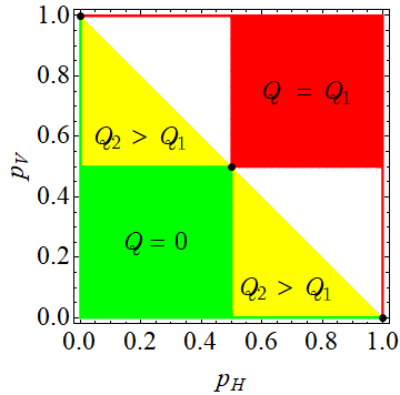
Figure 1: Dimensionless attenuation factors $p_{H}$ and $p_{V}$ for horizontally and vertically polarized photons for which the quantum channel (11) is degradable [red (dark gray) area], antidegradable [green (medium gray) area], both degradable and antidegradable (black points). Yellow (light gray) regions correspond to the coherent-information superadditivity detected with the use of two-letter encodings [23].

Consider a lossy quantum communication line such that the transmission coefficient for horizontally polarized photons, $p_{H}$, differs from that for vertically polarized photons, $p_{V}$. The simplest example is a horizontally oriented linear polarizer for which $p_{H}=1$ and $p_{V}=0$. In practice, however, all values $0\leq p_{H}\leq 1$ and $0\leq p_{V}\leq 1$ are attainable (see, e.g., [24]), which leads to a two-parameter family of qubit-to-qutrit channels

$$\!\!\!\!\!\Gamma\left[\left(\begin{array}[]{cc}\varrho_{HH}&\varrho_{HV}\\ \varrho_{VH}&\varrho_{VV}\\ \end{array}\right)\right]$$ (5)

$$\!\!\!\!\!=\left(\begin{array}[]{cc|c}p_{H}\varrho_{HH}&\sqrt{p_{H}p_{V}}\varrho_{HV}&0\\ \sqrt{p_{H}p_{V}}\varrho_{VH}&p_{V}\varrho_{VV}&0\\ \hline\cr 0&0&\begin{array}[]{c}(1-p_{H})\varrho_{HH}\\ +(1-p_{V})\varrho_{VV}\\ \end{array}\\ \end{array}\right),\quad$$ (11)

with $p_{H}$ and $p_{V}$ being the parameters. The extra (third) dimension in Eq. (11) corresponds to the vacuum contribution $|{\rm vac}\rangle$ that leads to no detector clicks. If $p_{H}=p_{V}$, then we get the standard erasure channel [25, 26]. If $p_{H}\neq p_{V}$, then Eq. (11) defines a generalized erasure channel [23] (cf. a similar but different concept in Ref. [14]) induced by the trace decreasing operation $\varrho\rightarrow\Lambda_{F}[\varrho]:=F\varrho F^{{\dagger}}$, where

$$F=\sqrt{p_{H}}|H\rangle\langle H|+\sqrt{p_{V}}|V\rangle\langle V|,$$

$|H\rangle$ and $|V\rangle$ are the single-photon states with horizontal and vertical polarization, respectively. The brief version of Eq. (11) is

$$\Gamma[\varrho]=F\varrho F^{{\dagger}}\oplus{\rm tr}[(I-F^{{\dagger}}F)\varrho]\,|{\rm vac}\rangle\langle{\rm vac}|.$$

The term ${\rm tr}[(I-F^{{\dagger}}F)\varrho]$ is the state dependent erasure probability. Denoting $G:=\sqrt{I-F^{{\dagger}}F}$ and recalling the notation $\Lambda_{G}[\varrho]:=G\varrho G^{{\dagger}}$, the channel (11) takes the form

$$\Gamma=\Lambda_{F}\oplus({\rm Tr}\circ\Lambda_{G}),$$ (12)

where ${\rm Tr}$ denotes the trash-and-prepare map $\varrho\rightarrow{\rm tr}[\varrho]\,|{\rm vac}\rangle\langle{\rm vac}|$. Interestingly, a complementary channel $\widetilde{\Gamma}$ can be expressed as [23]

$$\widetilde{\Gamma}=\Lambda_{G}\oplus({\rm Tr}\circ\Lambda_{F}),$$

which is equivalent to the change $p_{H}\rightarrow 1-p_{H}$ and $p_{V}\rightarrow 1-p_{V}$ in Eq. (11).

The fact that $\Gamma$ and $\widetilde{\Gamma}$ have the same structure was used in Ref. [23] to prove that $\Gamma$ is antidegradable [so that $Q(\Gamma)=0$] if and only if $\max(p_{H},p_{V})\leq\frac{1}{2}$ or $p_{H}=0$ or $p_{V}=0$, see the green (medium gray) region in Fig. 1. It was also shown in Ref. [23] that $Q(\Gamma)>0$ beyond the antidegradability region. $\Gamma$ is degradable [so that $Q(\Gamma)=Q_{1}(\Gamma)$] if and only if $\min(p_{H},p_{V})\geq\frac{1}{2}$ or $p_{H}=1$ or $p_{V}=1$, see the red (dark gray) region in Fig. 1. The final result of Ref. [23] is the analytical proof of superadditivity relation $Q_{2}(\Gamma)>Q_{1}(\Gamma)$ for two regions of attenuation factors: (i) $\frac{1}{2}<p_{H}<1$ and $0<p_{V}<1-p_{H}$, (ii) $\frac{1}{2}<p_{V}<1$ and $0<p_{H}<1-p_{V}$; see the yellow (light gray) areas in Fig. 1. White regions in Fig. 1 are terra incognita, where neither the degradability nor the antidegradability holds, and no strategies are known to outperform the one-shot capacity $Q_{1}(\Gamma)$.

The goal of this paper is twofold. First, we are going to close the gap in our understanding of the coherent-information superadditivity region in Fig. 1. To do so we provide some physically motivated $n$-partite entangled states $\varrho^{(n)}$, using which the coherent-information superadditivity region extends further and completely covers the white area in Fig. 1 in the limit $n\rightarrow\infty$. This result is interesting per se as it presents an analytical proof of the coherent-information superadditivity for an arbitrary $n\geq 2$. Second, for fixed values of $p_{H}$ and $p_{V}$, we are interested in finding particular states $\varrho^{(n)}$ leading to higher values of the coherent information. In this regard, we propose a scheme enabling one to get a higher quantum communication rate by doubling the number of channel uses.

II Superadditivity identification

Technically, it is quite difficult to maximize the coherent information $I_{c}(\varrho^{(n)},\Gamma^{\otimes n})$ with respect to $n$-qubit density operators $\varrho^{(n)}$ even if $p_{H}$, $p_{V}$, and $n$ are all fixed. In the case of the one-shot capacity ($n=1$), the optimal state $\varrho_{\rm opt}^{(1)}$ is shown to be diagonal in the basis $|H\rangle$, $|V\rangle$ for all $p_{H}$ and $p_{V}$, i.e.,

$$\varrho_{\rm opt}^{(1)}=\varrho_{HH}|H\rangle\langle H|+\varrho_{VV}|V\rangle\langle V|;$$

however, a closed-form expression for the coefficients $\varrho_{HH}$ and $\varrho_{VV}$ is still missing so they appear as a solution of some equation that can be readily solved numerically [23]. If $\Gamma$ is not antidegradable, then both $\varrho_{HH}>0$ and $\varrho_{VV}>0$ so that $Q_{1}(\Gamma)=I_{c}(\varrho_{\rm opt}^{(1)},\Gamma)>0$. Therefore, a random subspace code to attain $Q_{1}(\Gamma)$ does not need to exploit superpositions of horizontally and vertically polarized photons in its ensemble states. If the degradability property holds for $\Gamma$ [see the red (dark gray) region in Fig. 1], then $Q(\Gamma)=Q_{1}(\Gamma)=\frac{1}{n}I_{c}\left((\varrho_{\rm opt}^{(1)}))^{\otimes n},\Gamma^{\otimes n}\right)$ and there is no need nor benefit to consider states $\varrho^{(n)}$ other than $(\varrho_{\rm opt}^{(1)}))^{\otimes n}$. If $\Gamma$ is neither degradable nor antidegradable, then there is a potential for improvement. In Section II.1, we review in detail an approach of Ref. [23] to find a two-qubit state $\varrho^{(2)}$ outperforming $(\varrho_{\rm opt}^{(1)}))^{\otimes 2}$ in value of the two-shot coherent information $I_{c}(\varrho,\Gamma^{\otimes 2})$ for some parameters $p_{H}$ and $p_{V}$. In Section II.2, we generalize that approach to lower bound the $n$-shot quantum capacity $Q_{n}(\Gamma)$ for an arbitrary number $n$ of channel uses.

II.1 Two-shot capacity

Suppose $n=2$. Consider the state

$$\varrho^{(2)} = \big{(}\varrho_{\rm opt}^{(1)}\big{)}^{\otimes 2}+\varrho_{HH}\varrho_{VV}\left(|HV\rangle\langle VH|+|VH\rangle\langle HV|\right)$$ (13)

$$= \varrho_{HH}^{2}|HH\rangle\langle HH|+\varrho_{VV}^{2}|VV\rangle\langle VV|$$

$$+2\varrho_{HH}\varrho_{VV}\frac{|HV\rangle+|VH\rangle}{\sqrt{2}}\,\frac{\langle HV|+\langle VH|}{\sqrt{2}}.$$

Clearly, the diagonals of density matrices $\varrho^{(2)}$ and $(\varrho_{\rm opt}^{(1)})^{\otimes 2}$ coincide in the standard basis $(|HH\rangle,|HV\rangle,|VH\rangle,|VV\rangle)$. The two photon states $|HV\rangle$ and $|VH\rangle$ experience the same attenuation even if $p_{H}\neq p_{V}$ due to the obvious symmetry. In fact, all vectors from the subspace ${\cal H}_{1,1}:={\rm Span}(|HV\rangle,|VH\rangle)$ are equally attenuated, which makes it easy to calculate the output state

$$\!\!\!\!\!\Gamma^{\otimes 2}[\varrho^{(2)}]$$

$$\!\!\!\!\!=\big{(}\Gamma[\varrho_{\rm opt}^{(1)}]\big{)}^{\otimes 2}+p_{H}p_{V}\varrho_{HH}\varrho_{VV}\left(|HV\rangle\langle VH|+|VH\rangle\langle HV|\right)$$

$$\!\!\!\!\!=p_{H}^{2}\varrho_{HH}^{2}|HH\rangle\langle HH|+p_{V}^{2}\varrho_{VV}^{2}|VV\rangle\langle VV|$$

$$\!\!\!\!\!+2p_{H}p_{V}\varrho_{HH}\varrho_{VV}\frac{|HV\rangle+|VH\rangle}{\sqrt{2}}\,\frac{\langle HV|+\langle VH|}{\sqrt{2}}$$

$$\!\!\!\!\!+\big{(}(1-p_{H})\varrho_{HH}+(1-p_{V})\varrho_{VV}\big{)}$$

$$\quad\times\left(\varrho_{\rm opt}^{(1)}\otimes|{\rm vac}\rangle\langle{\rm vac}|+|{\rm vac}\rangle\langle{\rm vac}|\otimes\varrho_{\rm opt}^{(1)}\right)$$

$$\!\!\!\!\!+\big{(}(1-p_{H})\varrho_{HH}+(1-p_{V})\varrho_{VV}\big{)}^{2}|{\rm vac}\rangle\langle{\rm vac}|\otimes|{\rm vac}\rangle\langle{\rm vac}|.$$

The density operators $\Gamma^{\otimes 2}[\varrho^{(2)}]$ and $\big{(}\Gamma[\varrho_{\rm opt}^{(1)}]\big{)}^{\otimes 2}$ differ by their action in the subspace ${\cal H}_{1,1}$, namely, $\Gamma^{\otimes 2}[\varrho^{(2)}]$ acts as a coherent operator

$$2p_{H}p_{V}\varrho_{HH}\varrho_{VV}\frac{|HV\rangle+|VH\rangle}{\sqrt{2}}\,\frac{\langle HV|+\langle VH|}{\sqrt{2}},$$ (14)

whereas $\big{(}\Gamma[\varrho_{\rm opt}^{(1)}]\big{)}^{\otimes 2}$ acts as an incoherent operator

$$p_{H}p_{V}\varrho_{HH}\varrho_{VV}(|HV\rangle\langle HV|+|VH\rangle\langle VH|).$$ (15)

This leads to a readily accountable difference in spectra of the two states. Spectrum of (14) is $(2p_{H}p_{V}\varrho_{HH}\varrho_{VV},0)$ and that of (15) is $(p_{H}p_{V}\varrho_{HH}\varrho_{VV},p_{H}p_{V}\varrho_{HH}\varrho_{VV})$. We have

$$S(\Gamma^{\otimes 2}[\varrho^{(2)}]) = S\Big{(}(\Gamma[\varrho_{\rm opt}^{(1)}])^{\otimes 2}\Big{)}$$

$$-(2\log 2)p_{H}p_{V}\varrho_{HH}\varrho_{VV}.$$

As the complementary channel $\widetilde{\Gamma}$ is obtained from the direct channel $\Gamma$ by the change $p_{H}\rightarrow 1-p_{H}$ and $p_{V}\rightarrow 1-p_{V}$, we readily have

$$S(\widetilde{\Gamma}^{\otimes 2}[\varrho^{(2)}]) = S\Big{(}(\widetilde{\Gamma}[\varrho_{\rm opt}^{(1)}])^{\otimes 2}\Big{)}$$

$$-(2\log 2)(1-p_{H})(1-p_{V})\varrho_{HH}\varrho_{VV}.$$

Finally, we get

$$I_{c}(\varrho^{(2)},\Gamma^{\otimes 2})=S(\Gamma^{\otimes 2}[\varrho^{(2)}])-S(\widetilde{\Gamma}^{\otimes 2}[\varrho^{(2)}])$$

$$=S\Big{(}\big{(}\Gamma[\varrho_{\rm opt}^{(1)}]\big{)}^{\otimes 2}\Big{)}-S\Big{(}\big{(}\widetilde{\Gamma}[\varrho_{\rm opt}^{(1)}]\big{)}^{\otimes 2}\Big{)}$$

$$\quad+(2\log 2)(1-p_{H}-p_{V})\varrho_{HH}\varrho_{VV}$$

$$=2I_{c}(\varrho_{\rm opt}^{(1)},\Gamma)+(2\log 2)(1-p_{H}-p_{V})\varrho_{HH}\varrho_{VV}$$

$$=2Q_{1}(\Gamma)+(2\log 2)(1-p_{H}-p_{V})\varrho_{HH}\varrho_{VV}.$$ (16)

The coherent information is superadditive if $(1-p_{H}-p_{V})\varrho_{HH}\varrho_{VV}>0$, i.e., if $p_{H}+p_{V}<1$ and the state $\varrho_{\rm opt}^{(1)}$ is nondegenerate. The latter condition is fulfilled if $\Gamma$ is not antidegradable. Combining these conditions we get two yellow (light gray) regions in Fig. 1, where

$$Q_{2}(\Gamma)\geq\frac{1}{2}I_{c}(\varrho^{(2)},\Gamma^{\otimes 2})>Q_{1}(\Gamma).$$

II.2 $n$-shot capacity

Suppose $n>2$. A generalization of the approach in Section II.1 would be to consider a state $(\varrho_{\rm opt}^{(1)})^{\otimes n}$ and modify it to a state $\varrho^{(n)}$, which would differ from $(\varrho_{\rm opt}^{(1)})^{\otimes n}$ when acting on some subspace that is symmetric with respect to permutations of photons. Physically, the subspace is to be chosen in such a way as to ensure a high enough detection probability for all states from the subspace. Suppose $p_{H}>p_{V}$, then the state $|H\rangle^{\otimes n}$ has the highest detection probability, but the corresponding subspace ${\cal H}_{n,0}:={\rm Span}(|H\rangle^{\otimes n})$ is trivial (has dimension $1$). So we consider the subspace ${\cal H}_{n-1,1}$ spanned by the vector $|H\rangle^{\otimes(n-1)}\otimes|V\rangle$ and all its photon-permuted versions. The detection probability for all states from this subspace equals $p_{H}^{n-1}p_{V}$. The following entangled $n$-qubit $W$-state belongs to ${\cal H}_{n-1,1}$:

$$|W^{(n)}\rangle=\frac{1}{\sqrt{n}} \Big{(} |\underbrace{HH\ldots HH}_{n-1}V\rangle$$ (17)

$$+ |\underbrace{HH\ldots H}_{n-2}VH\rangle$$

$$+ \ldots$$

$$+ |V\underbrace{H\ldots HHH}_{n-1}\rangle\Big{)}\in{\cal H}_{n-1,1}.$$

Consider the $n$-qubit density operator $\varrho^{(n)}$ defined through

$$\varrho^{(n)}|\varphi\rangle=\left\{\begin{array}[]{ll}(\varrho_{\rm opt}^{(1)})^{\otimes n}|\varphi\rangle&\text{if~{}}|\varphi\rangle\perp{\cal H}_{n-1,1},\\ n\varrho_{HH}^{n-1}\varrho_{VV}|W^{(n)}\rangle\langle W^{(n)}||\varphi\rangle&\text{if~{}}|\varphi\rangle\in{\cal H}_{n-1,1}.\\ \end{array}\right.$$

The restriction of $\varrho^{(n)}$ to the subspace ${\cal H}_{n-1,1}$ is a coherent (rank-1) operator

$$\lfloor\varrho^{(n)}\rfloor_{{\cal H}_{n-1,n}}:=n\varrho_{HH}^{n-1}\varrho_{VV}|W^{(n)}\rangle\langle W^{(n)}|,$$ (18)

whereas the restriction of $(\varrho_{\rm opt}^{(1)})^{\otimes n}$ to the subspace ${\cal H}_{n-1,1}$ is a mixed (rank-$n$) operator

$$\lfloor(\varrho_{\rm opt}^{(1)})^{\otimes n}\rfloor_{{\cal H}_{n-1,n}}$$

$$:=\varrho_{HH}^{n-1}\varrho_{VV}\Big{(}|\underbrace{HH\ldots HH}_{n-1}V\rangle\langle\underbrace{HH\ldots HH}_{n-1}V|$$

$$\qquad\qquad\qquad+|\underbrace{HH\ldots H}_{n-2}VH\rangle\langle\underbrace{HH\ldots H}_{n-2}VH|$$

$$\qquad\qquad\qquad+\ldots$$

$$\qquad\qquad\qquad+|V\underbrace{H\ldots HHH}_{n-1}\rangle\langle V\underbrace{H\ldots HHH}_{n-1}|\Big{)},\qquad$$ (19)

but beyond that restriction

$$\varrho^{(n)}-\lfloor\varrho^{(n)}\rfloor_{{\cal H}_{n-1,n}}=(\varrho_{\rm opt}^{(1)})^{\otimes n}-\lfloor(\varrho_{\rm opt}^{(1)})^{\otimes n}\rfloor_{{\cal H}_{n-1,n}}.$$

Using the direct sum representation (12) of the channel $\Gamma$, we explicitly find its tensor power

$$\Gamma^{\otimes n} = \Lambda_{F}^{\otimes n}\oplus\ldots$$ (20)

$$\oplus\underbrace{\left[\Lambda_{F}^{\otimes(n-k)}\otimes({\rm Tr}\circ\Lambda_{G})^{\otimes k}\right]\oplus\ldots}_{\binom{n}{k}\text{~{}terms}}$$

$$\oplus\ldots\oplus({\rm Tr}\circ\Lambda_{G})^{\otimes n},$$

where the brace denotes a direct sum of $\binom{n}{k}$ different terms, with each term being a permuted tensor product of $n-k$ maps $\Lambda_{F}$ and $k$ maps ${\rm Tr}\circ\Lambda_{G}$. Let us consider how the term $\Lambda_{F}^{\otimes(n-k)}\otimes({\rm Tr}\circ\Lambda_{G})^{\otimes k}$ affects the operators $\lfloor\varrho^{(n)}\rfloor_{{\cal H}_{n-1,n}}$ and $\lfloor(\varrho_{\rm opt}^{(1)})^{\otimes n}\rfloor_{{\cal H}_{n-1,n}}$. Recalling the effect of the partial trace on $W$-states, we see that the coherent component of $\Lambda_{F}^{\otimes(n-k)}\otimes({\rm Tr}\circ\Lambda_{G})^{\otimes k}\big{[}\lfloor\varrho^{(n)}\rfloor_{{\cal H}_{n-1,n}}\big{]}$ reads

$$\varrho_{HH}^{n-1}\varrho_{VV}\,p_{H}^{n-k-1}p_{V}(1-p_{H})^{k}$$

$$\times(n-k)|W^{(n-k)}\rangle\langle W^{(n-k)}|\otimes(|{\rm vac}\rangle\langle{\rm vac}|)^{\otimes k},\qquad$$ (21)

whereas $\Lambda_{F}^{\otimes(n-k)}\otimes({\rm Tr}\circ\Lambda_{G})^{\otimes k}\big{[}\lfloor(\varrho_{\rm opt}^{(1)})^{\otimes n}\rfloor_{{\cal H}_{n-1,n}}\big{]}$ has the completely incoherent component

$$\varrho_{HH}^{n-1}\varrho_{VV}\,p_{H}^{n-k-1}p_{V}(1-p_{H})^{k}$$

$$\times\Big{(}|\underbrace{HH\ldots HH}_{n-k-1}V\rangle\langle\underbrace{HH\ldots HH}_{n-k-1}V|$$

$$\qquad+|\underbrace{HH\ldots H}_{n-k-2}VH\rangle\langle\underbrace{HH\ldots H}_{n-k-2}VH|$$

$$\qquad+\ldots$$

$$\qquad+|V\underbrace{H\ldots HHH}_{n-k-1}\rangle\langle V\underbrace{H\ldots HHH}_{n-k-1}|\Big{)}$$

$$\otimes(|{\rm vac}\rangle\langle{\rm vac}|)^{\otimes k}.$$ (22)

The operator (21) has the only nonzero eigenvalue, whereas the operator (22) has $n-k$ coincident nonzero eigenvalues, with traces of the two operators being the same. Therefore, the only nonzero eigenvalue of the operator (21) is $(n-k)$ multiplied by any nonzero eigenvalue of the operator (22). This leads to a simple expression for the difference in entropies, namely,

$$\!\!\!\!\!S\Big{(}\Lambda_{F}^{\otimes(n-k)}\otimes({\rm Tr}\circ\Lambda_{G})^{\otimes k}[\varrho^{(n)}]\Big{)}$$

$$\!\!\!\!\!=S\Big{(}\Lambda_{F}^{\otimes(n-k)}\otimes({\rm Tr}\circ\Lambda_{G})^{\otimes k}[(\varrho_{\rm opt}^{(1)})^{\otimes n}]\Big{)}$$

$$\!\!\!\!\!\quad-\varrho_{HH}^{n-1}\varrho_{VV}\,p_{V}p_{H}^{n-k-1}(1-p_{H})^{k}\,(n-k)\log(n-k).\qquad$$ (23)

Since the operators (18) and (19) are invariant with respect to permutations of photons, each term in the brace in Eq. (20) results in the same entropy decrement as in Eq. (II.2). Summing all the decrements, we get

$$\!\!\!\!\!S\Big{(}\Gamma^{\otimes n}[\varrho^{(n)}]\Big{)}=S\Big{(}\Gamma^{\otimes n}[(\varrho_{\rm opt}^{(1)})^{\otimes n}]\Big{)}-\varrho_{HH}^{n-1}\varrho_{VV}$$

$$\!\!\!\!\!\times\sum_{k=0}^{n-1}\binom{n}{k}\,p_{V}p_{H}^{n-k-1}(1-p_{H})^{k}\,(n-k)\log(n-k).$$

Similarly, for the complementary channel we have

$$\!\!\!\!\!S\Big{(}\widetilde{\Gamma}^{\otimes n}[\varrho^{(n)}]\Big{)}=S\Big{(}\widetilde{\Gamma}^{\otimes n}[(\varrho_{\rm opt}^{(1)})^{\otimes n}]\Big{)}-\varrho_{HH}^{n-1}\varrho_{VV}$$

$$\!\!\!\!\!\times\sum_{k=0}^{n-1}\binom{n}{k}\,(1-p_{V})(1-p_{H})^{n-k-1}p_{H}^{k}\,(n-k)\log(n-k).$$

Finally, we get

$$\!\!\!\!\!\!\!\!\!\!Q_{n}(\Gamma)-Q_{1}(\Gamma)\geq\frac{1}{n}\left[I_{c}(\varrho^{(n)},\Gamma^{\otimes n})-I_{c}\big{(}(\varrho_{\rm opt}^{(1)})^{\otimes n},\Gamma^{\otimes n}\big{)}\right]$$

$$\!\!\!\!\!\!\!\!\!\!=\frac{1}{n}\varrho_{HH}^{n-1}\varrho_{VV}\sum_{k=0}^{n-1}\binom{n}{k}(n-k)\log(n-k)$$

$$\!\!\!\!\!\!\!\!\!\!\quad\times\left[(1-p_{V})(1-p_{H})^{n-k-1}p_{H}^{k}-p_{V}p_{H}^{n-k-1}(1-p_{H})^{k}\right]$$

$$\!\!\!\!\!\!\!\!\!\!=\varrho_{HH}^{n-1}\varrho_{VV}\sum_{k=0}^{n-1}\binom{n-1}{k}\log(n-k)$$

$$\!\!\!\!\!\!\!\!\!\!\quad\times\left[(1-p_{V})(1-p_{H})^{n-k-1}p_{H}^{k}-p_{V}p_{H}^{n-k-1}(1-p_{H})^{k}\right]$$

$$\!\!\!\!\!\!\!\!\!\!=\varrho_{HH}^{n-1}\varrho_{VV}\sum_{k=0}^{n-1}\binom{n-1}{k}(1-p_{H})^{n-k-1}p_{H}^{k}$$

$$\!\!\!\!\!\!\!\!\!\!\quad\times\left[(1-p_{V})\log(n-k)-p_{V}\log(k+1)\right].$$ (24)

If the obtained expression (24) is positive, then we successfully identify the coherent-information superadditivity in the form $Q_{n}(\Gamma)>Q_{1}(\Gamma)$. Suppose $\Gamma$ is not antidegradable, then $\varrho_{HH}>0$, $\varrho_{VV}>0$, and $Q_{n}(\Gamma)>Q_{1}(\Gamma)$ if the sum in Eq. (24) is positive.

In the above analysis, we assumed $p_{H}>p_{V}$. The converse case $p_{V}>p_{H}$ obviously reduces to the considered one if we replace $|H\rangle\leftrightarrow|V\rangle$ in Eq. (17). Therefore, we make the following conclusion: $Q_{n}(\Gamma)>Q_{1}(\Gamma)$ if $\Gamma$ is not antidegradable and $w_{n}(p_{H},p_{V})>0$, where

$$w_{n}(p_{H},p_{V}):=\sum\limits_{k=0}^{n-1}\binom{n-1}{k}(1-p_{H})^{n-k-1}p_{H}^{k}$$

$$\qquad\times\left[(1-p_{V})\log(n-k)-p_{V}\log(k+1)\right]$$ (25)

if $p_{H}>p_{V}$,

$$w_{n}(p_{H},p_{V}):=\sum\limits_{k=0}^{n-1}\binom{n-1}{k}(1-p_{V})^{n-k-1}p_{V}^{k}$$

$$\qquad\times\left[(1-p_{H})\log(n-k)-p_{H}\log(k+1)\right]$$ (26)

if $p_{V}>p_{H}$.

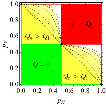
Figure 2: Nested superadditivity regions $Q_{n}(\Gamma)>Q_{1}(\Gamma)$ [yellow (light gray) areas] in the parameter space (dimensionless attenuation factors $p_{H}$ and $p_{V}$ for horizontally and vertically polarized photons) with boundaries depicted for various values: $n=2$ (dotted line), $n=3,10,10^{2},10^{3},10^{4}$ (dashed lines from left to right).

In the case $n=2$, the condition $w_{2}(p_{H},p_{V})>0$ is equivalent to $p_{H}+p_{V}<1$, i.e., we reproduce the results of Section II.1. If $n\geq 3$, then the region of parameters $p_{H}$ and $p_{V}$, where $Q_{n}(\Gamma)>Q_{1}(\Gamma)$, is strictly larger than the region, where $Q_{2}(\Gamma)>Q_{1}(\Gamma)$, see Fig. 2. Interestingly, the greater $n$ the larger the region, where $Q_{n}(\Gamma)>Q_{1}(\Gamma)$. If $n=10^{4}$, then the condition $w_{10^{4}}(p_{H},p_{V})>0$ defines a region in the plane $(p_{H},p_{V})$, which almost coincides with the area where $\Gamma$ is neither degradable nor antidegradable (see Fig. 2). This observation motivates us to study the asymptotic behaviour of $w_{n}(p_{H},p_{V})$.

The binomial distribution $\{\binom{n-1}{k}(1-p)^{n-k-1}p^{k}\}_{k=0}^{n-1}$ tends to the normal distribution ${\cal N}(np,np(1-p))$ with the mean value $np$ and the standard deviation $\sqrt{np(1-p)}$ when $0<p<1$ and $n$ tends to infinity [27]. Therefore, the terms with $k\approx np_{H}$ contribute the most to Eq. (25) and the terms with $k\approx np_{V}$ contribute the most to Eq. (26). In the asymptotic limit $n\rightarrow\infty$ we have

$$w_{n}(p_{H},p_{V}) \approx (1-2p_{V})\log n+(1-p_{V})\log(1-p_{H})$$ (27)

$$-p_{V}\log p_{H}\text{~{}if~{}}p_{H}>p_{V},$$

$$w_{n}(p_{H},p_{V}) \approx (1-2p_{H})\log n+(1-p_{H})\log(1-p_{V})$$ (28)

$$-p_{H}\log p_{V}\text{~{}if~{}}p_{V}>p_{H}.$$

Hence, $w_{n}(p_{H},p_{V})>0$ in the asymptotic limit $n\rightarrow\infty$ if $0<p_{V}<\frac{1}{2}<p_{H}<1$ or $0<p_{H}<\frac{1}{2}<p_{V}<1$, which is exactly the region, where $\Gamma$ is neither degradable nor antidegradable (see Fig. 2).

Suppose the parameters $p_{H}$ and $p_{V}$ are fixed. Exploiting the asymptotic formulas (27)–(28) and solving the inequality $w_{n}(p_{H},p_{V})\geq 0$, we estimate the number $n$ needed to observe the superadditivity phenomenon $Q_{n}>Q_{1}$:

$$n\gtrsim n_{0}:=\left\{\begin{array}[]{ll}\left(\frac{p_{H}^{p_{V}}}{(1-p_{H})^{1-p_{V}}}\right)^{\frac{1}{1-2p_{V}}}&\text{if~{}}0<p_{V}<\frac{1}{2}<p_{H}<1,\\ \left(\frac{p_{V}^{p_{H}}}{(1-p_{V})^{1-p_{H}}}\right)^{\frac{1}{1-2p_{H}}}&\text{if~{}}0<p_{H}<\frac{1}{2}<p_{V}<1.\\ \end{array}\right.$$

If $n\gg n_{0}$, then the proposed states yields the following benefit in the quantum communication rate:

$$\frac{1}{n}I_{c}(\varrho^{(n)},\Gamma^{\otimes n})\approx Q_{1}(\Gamma)$$

$$+\left\{\begin{array}[]{ll}(1-2p_{V})\varrho_{HH}^{n-1}\varrho_{VV}\log n&\text{if~{}}0<p_{V}<\frac{1}{2}<p_{H}<1,\\ (1-2p_{H})\varrho_{HH}\varrho_{VV}^{n-1}\log n&\text{if~{}}0<p_{H}<\frac{1}{2}<p_{V}<1.\\ \end{array}\right.$$

III Superadditivity improvement

The goal of the previous section was to detect the coherent-information superadditivity in the widest region of parameters $p_{H}$ and $p_{V}$. In this section we discuss how to get a higher quantum communication rate (for fixed values of $p_{H}$ and $p_{V}$) by using the channel multiple times.

Our approach is to combine two $n$-qubit states $\varrho^{(n)}$ from Section II and slightly modify them to get a better $2n$-qubit state $\xi^{(2n)}$. To illustrate this approach, consider the region $0<p_{V}<1-p_{H}<\frac{1}{2}$, where $Q_{2}>Q_{1}$ (see Section II.1). Let $\varrho^{(2)}$ be a partially coherent state given by Eq. (13). The four-qubit state $\varrho^{(2)}\otimes\varrho^{(2)}$ inherits some superpositions in the subspace spanned by 12 vectors: $|HHHV\rangle$, $|HHVH\rangle$, $|HVHH\rangle$, $|HVHV\rangle$, $|HVVH\rangle$, $|HVVV\rangle$, $|VHHH\rangle$, $|VHHV\rangle$, $|VHVH\rangle$, $|VHVV\rangle$, $|VVHV\rangle$, and $|VVVH\rangle$. On the other hand, the states $|HHVV\rangle$ and $|VVHH\rangle$ incoherently contribute to $\varrho^{(2)}\otimes\varrho^{(2)}$ though they have the same detection probability $p_{H}^{2}p_{V}^{2}$. We use the latter fact to construct a more coherent version of the state $\varrho^{(2)}\otimes\varrho^{(2)}$ as follows:

$$\xi^{(4)} := \varrho^{(2)}\otimes\varrho^{(2)}+\varrho_{HH}^{2}\varrho_{VV}^{2}(|HHVV\rangle\langle VVHH|$$

$$\qquad\qquad\qquad\qquad+|VVHH\rangle\langle HHVV|).\quad$$

The states $\varrho^{(2)}\otimes\varrho^{(2)}$ and $\xi^{(4)}$ have the almost identical spectra, with the difference being in the eigenspace spanned by $|HHVV\rangle$ and $|VVHH\rangle$. That difference is translated into the operators $\Lambda_{F}^{\otimes 4}[\xi^{(4)}]$ and $\Lambda_{F}^{\otimes 4}[\varrho^{(2)}\otimes\varrho^{(2)}]$, which results in

$$S(\Lambda_{F}^{\otimes 4}[\xi^{(4)}])=S(\Lambda_{F}^{\otimes 4}[\varrho^{(2)}\otimes\varrho^{(2)}])-(2\log 2)p_{H}^{2}p_{V}^{2}\varrho_{HH}^{2}\varrho_{VV}^{2}.$$

Since the partial trace of the operator $(|HHVV\rangle\langle VVHH|+|VVHH\rangle\langle HHVV|)$ with respect to any photon vanishes, this means that $\Lambda_{F}^{\otimes 3}\otimes({\rm Tr}\circ\Lambda_{G})[\xi^{(4)}]=\Lambda_{F}^{\otimes 3}\otimes({\rm Tr}\circ\Lambda_{G})[\varrho^{(2)}\otimes\varrho^{(2)}]$, etc., so that the density operators $\xi^{(4)}$ and $\varrho^{(2)}\otimes\varrho^{(2)}$ are both mapped to the same operator when affected by any map involving the trash-and-prepare operation ${\rm Tr}$ for at least one of the qubits. Recalling the fact that $\Gamma^{\otimes 4}=[\Lambda_{F}\oplus({\rm Tr}\circ\Lambda_{G})]^{\otimes 4}$, we get

$$S(\Gamma^{\otimes 4}[\xi^{(4)}])=S(\Gamma^{\otimes 4}[\varrho^{(2)}\otimes\varrho^{(2)}])-(2\log 2)p_{H}^{2}p_{V}^{2}\varrho_{HH}^{2}\varrho_{VV}^{2}.$$

Similarly,

$$S(\widetilde{\Gamma}^{\otimes 4}[\xi^{(4)}]) = S(\widetilde{\Gamma}^{\otimes 4}[\varrho^{(2)}\otimes\varrho^{(2)}])$$

$$-(2\log 2)(1-p_{H})^{2}(1-p_{V})^{2}\varrho_{HH}^{2}\varrho_{VV}^{2}.$$

These relations lead to a greater coherent information as compared to twice the expression (16), namely,

$$I_{c}(\xi^{(4)},\Gamma^{\otimes 4})=S(\Gamma^{\otimes 4}[\xi^{(4)}])-S(\widetilde{\Gamma}^{\otimes 4}[\xi^{(4)}])$$

$$=S(\Gamma^{\otimes 4}[\varrho^{(2)}\otimes\varrho^{(2)}])-S(\widetilde{\Gamma}^{\otimes 4}[\varrho^{(2)}\otimes\varrho^{(2)}])$$

$$\quad+(2\log 2)\varrho_{HH}^{2}\varrho_{VV}^{2}[(1-p_{H})^{2}(1-p_{V})^{2}-p_{H}^{2}p_{V}^{2}]$$

$$=2I_{c}(\varrho^{(2)},\Gamma^{\otimes 2})$$

$$\quad+(2\log 2)\varrho_{HH}^{2}\varrho_{VV}^{2}[(1-p_{H})^{2}(1-p_{V})^{2}-p_{H}^{2}p_{V}^{2}]$$

$$=4Q_{1}(\Gamma)+(4\log 2)\varrho_{HH}\varrho_{VV}(1-p_{H}-p_{V})$$

$$\quad+(2\log 2)\varrho_{HH}^{2}\varrho_{VV}^{2}[(1-p_{H})^{2}(1-p_{V})^{2}-p_{H}^{2}p_{V}^{2}].\qquad$$ (30)

Dividing Eq. (30) by 4, we get a better lower bound

$$Q_{4}(\Gamma)-Q_{1}(\Gamma)\geq\frac{1}{4}I_{c}(\xi^{(4)},\Gamma^{\otimes 4})-Q_{1}(\Gamma)$$

$$=\left[1+\frac{1}{2}\varrho_{HH}\varrho_{VV}(1-p_{H}-p_{V}+2p_{H}p_{V})\right]$$

$$\times(\log 2)(1-p_{H}-p_{V})\varrho_{HH}\varrho_{VV}.$$ (31)

The lower bound (31) significantly outperforms the lower bound (24) for $n=4$ in a wide range of parameters $p_{H}$ and $p_{V}$. For instance, if $p_{H}=0.7$ and $p_{V}=0.2$, then Eq. (31) yields $Q_{4}(\Gamma)-Q_{1}(\Gamma)\geq 6.3\times 10^{-3}$ bits, whereas Eq. (24) yields $Q_{4}(\Gamma)-Q_{1}(\Gamma)\geq 9.1\times 10^{-5}$ bits.

Clearly, the presented approach works well to extend the $n$-qubit state $\varrho^{(n)}$ from Section II.2 to a $2n$-qubit state $\xi^{(2n)}$ by modifying the state $(\varrho^{(n)})^{\otimes 2}$ in the subspace spanned by $|H\rangle^{\otimes n}\otimes|V\rangle^{\otimes n}$ and $|V\rangle^{\otimes n}\otimes|H\rangle^{\otimes n}$. Similarly, the modified $2n$-qubit state $\xi^{(2n)}$ can further be improved to a $4n$-qubit state and so on ad infinitum. Starting with the two-qubit state in Section II.1, we get the following result:

$$Q(\Gamma)-Q_{1}(\Gamma)\geq(\log 2)(1-p_{H}-p_{V})\sum\limits_{m=0}^{\infty}\frac{\varrho_{HH}^{2^{m}}\varrho_{VV}^{2^{m}}}{2^{m}}$$

$$\qquad\qquad\times\sum\limits_{k=0}^{2^{m}-1}(1-p_{H})^{2^{m}-k-1}(1-p_{V})^{2^{m}-k-1}p_{H}^{k}p_{V}^{k}.$$

IV Conclusions

A phenomenon of the coherent-information superadditivity makes it possible to enhance the quantum communication rate by using clever codes. In this paper, we have studied the superadditivity phenomenon in physically relevant quantum communication lines with polarization dependent losses. Such lines represent a two-parameter family of generalized erasure channels $\Gamma$, with the attenuation factors $p_{H}$ and $p_{V}$ for horizontally and vertically polarized photons being the parameters. In prior research, two-shot capacity $Q_{2}(\Gamma)$ was shown to be greater than the one-shot capacity $Q_{1}(\Gamma)$ for some values of $p_{H}$ and $p_{V}$ within the region $p_{H}+p_{V}<1$ [23]. Interestingly, if $p_{H}+p_{V}\geq 1$, then $\Gamma$ is input-degradable in the sense that there exists a quantum channel $\Upsilon$ such that $\widetilde{\Gamma}=\Gamma\circ\Upsilon$. Making an analogy with the case of standard degradable channels, it is tempting to conjecture that the input-degradability implies $Q_{n}(\Gamma)=Q_{1}(\Gamma)$ if $p_{H}+p_{V}\geq 1$. Our study shows that this conjecture is false: the 3-qubit state $\varrho^{(3)}$ in Section II.2 insures $Q_{3}(\Gamma)>Q_{1}(\Gamma)$ if $p_{H}+p_{V}=1$ and $0\neq p_{H}\neq p_{V}\neq 0$, see Fig. 2.

The more the number of channel uses in Section II.2 the wider the region of parameters $p_{H}$ and $p_{V}$, where the superadditivity phenomenon takes place. In the limit of infinitely many channel uses, we have proved the strict inequality $Q(\Gamma)>Q_{1}(\Gamma)$ for all $p_{H}$ and $p_{V}$ satisfying $0<p_{V}<\frac{1}{2}<p_{H}<1$ or $0<p_{H}<\frac{1}{2}<p_{V}<1$, i.e., $Q(\Gamma)>Q_{1}(\Gamma)$ whenever $\Gamma$ is neither degradable nor antidegradable. A feature of the state proposed in Section II.2 is that it has a clear physical meaning: $\varrho^{(n)}$ has an entangled component proportional to $|W^{(n)}\rangle\langle W^{(n)}|$, which in turn has a high detection probability and whose structure is preserved by polarization dependent losses due to the permutation symmetry. Clearly, one could alternatively use another Dicke state [28, 29] instead of $|W^{(n)}\rangle$; however, the detection probability would be less in that case.

In this work, we were interested not only in the superadditivity identification but also in its improvement with the increase of channel uses. In Section II.2, we proposed a method how to get a higher quantum communication rate by doubling the number of channel uses. We believe that the scheme is far from being optimal, which necessitates a further search of better codes, e.g., by using a neural network state ansatz [30, 31]. Nonetheless, our analytically derived states with known asymptotic values of coherent information may serve as a benchmark for future codes generated by numerical optimization.

- [1] R. Horodecki, P. Horodecki, M. Horodecki, and K. Horodecki, Quantum entanglement, Rev. Mod. Phys. 81, 865 (2009).
- [2] M. Erhard, M. Krenn, and A. Zeilinger, Advances in high-dimensional quantum entanglement, Nat. Rev. Phys. 2, 365 (2020).
- [3] S. Lloyd, Capacity of the noisy quantum channel, Phys. Rev. A 55, 1613 (1997).
- [4] H. Barnum, M. A. Nielsen, and B. Schumacher, Information transmission through a noisy quantum channel, Phys. Rev. A 57, 4153 (1998).
- [5] P. W. Shor, Quantum error correction, Lecture notes of MSRI Workshop on Quantum Information And Cryptography (November 4–8, 2002). Available at https://www.msri.org/workshops/203/schedules/1181.
- [6] I. Devetak, The private classical capacity and quantum capacity of a quantum channel, IEEE Transactions on Information Theory 51, 44 (2005).
- [7] M. M. Wilde, Quantum Information Theory (Cambridge University Press, Cambridge, 2013).
- [8] A. S. Holevo, Quantum Systems, Channels, Information. A Mathematical Introduction (de Gruyter, Berlin, Boston, 2012).
- [9] I. Devetak and P. Shor, The capacity of a quantum channel for simultaneous transmission of classical and quantum information, Commun. Math. Phys. 256, 287 (2005).
- [10] D. P. DiVincenzo, P. W. Shor, and J. A. Smolin, Quantum-channel capacity of very noisy channels, Phys. Rev. A 57, 830 (1998).
- [11] J. Fern and K. B. Whaley, Lower bounds on the nonzero capacity of Pauli channels, Phys. Rev. A 78, 062335 (2008).
- [12] F. Leditzky, D. Leung, and G. Smith, Dephrasure channel and superadditivity of coherent information, Phys. Rev. Lett. 121, 160501 (2018).
- [13] S. Yu, Y. Meng, R. B. Patel, Y.-T. Wang, Z.-J. Ke, W. Liu, Z.-P. Li, Y.-Z. Yang, W.-H. Zhang, J.-S. Tang, C.-F. Li, and G.-C. Guo, Experimental observation of coherent-information superadditivity in a dephrasure channel, Phys. Rev. Lett. 125, 060502 (2020).
- [14] V. Siddhu and R. B. Griffiths, Positivity and nonadditivity of quantum capacities using generalized erasure channels, IEEE Trans. Inform. Theory 67, 4533 (2021).
- [15] V. Siddhu, Leaking information to gain entanglement, arXiv:2011.15116.
- [16] F. Leditzky, D. Leung, V. Siddhu, G. Smith, J. A. Smolin, Generic nonadditivity of quantum capacity in simple channels, arXiv:2202.08377.
- [17] T. Cubitt, D. Elkouss, W. Matthews, M. Ozols, D. Pérez-García, and S. Strelchuk, Unbounded number of channel uses may be required to detect quantum capacity, Nature Commun. 6, 6739 (2015).
- [18] N. Gisin and B. Huttner, Combined effects of polarization mode dispersion and polarization dependent losses in optical fibers, Optics Communications 142, 119 (1997).
- [19] B. T. Kirby, D. E. Jones, and M. Brodsky, Effect of polarization dependent loss on the quality of transmitted polarization entanglement, Journal of Lightwave Technology 37, 95 (2019).
- [20] C. Li, M. Curty, F. Xu, O. Bedroya, and H.-K. Lo, Secure quantum communication in the presence of phase- and polarization-dependent loss, Phys. Rev. A 98, 042324 (2018).
- [21] S. N. Filippov, Trace decreasing quantum dynamical maps: Divisibility and entanglement dynamics, arXiv:2108.13372.
- [22] S. N. Filippov, Entanglement robustness in trace decreasing quantum dynamics, Quanta 10, 15 (2021).
- [23] S. N. Filippov, Capacity of trace decreasing quantum operations and superadditivity of coherent information for a generalized erasure channel, J. Phys. A: Math. Theor. 54, 255301 (2021).
- [24] I. Bongioanni, L. Sansoni, F. Sciarrino, G. Vallone, and P. Mataloni, Experimental quantum process tomography of non-trace-preserving maps, Phys. Rev. A 82, 042307 (2010).
- [25] M. Grassl, T. Beth, and T. Pellizzari, Codes for the quantum erasure channel, Phys. Rev. A 56, 33 (1997).
- [26] C. H. Bennett, D. P. DiVincenzo, and J. A. Smolin, Capacities of quantum erasure channels, Phys. Rev. Lett. 78, 3217 (1997).
- [27] Z. Govindarajulu, Normal approximations to the classical discrete distributions, Sankhyā: The Indian Journal of Statistics, Series A 27, 143 (1965).
- [28] R. H. Dicke, Coherence in spontaneous radiation processes, Phys. Rev. 93, 99 (1954).
- [29] X. Chen and L. Jiang, Noise tolerance of Dicke states, Phys. Rev. A 101, 012308 (2020).
- [30] J. Bausch and F. Leditzky, Quantum codes from neural networks, New J. Phys. 22, 023005 (2020).
- [31] G. L. Sidhardh, M. Alimuddin, M. Banik, Exploring super-additivity of coherent information of noisy quantum channels through genetic algorithms, arXiv:2201.03958.