Bounds on fluctuations for ensembles of quantum thermal machines

Abstract

We study universal aspects of fluctuations in an ensemble of noninteracting continuous quantum thermal machines in the steady state limit. Considering an individual machine, such as a refrigerator, in which relative fluctuations (and high order cumulants) of the cooling heat current to the absorbed heat current, $\eta^{(n)}$, are upper-bounded, $\eta^{(n)}\leq\eta_{C}^{n}$ with $n\geq 2$ and $\eta_{C}$ the Carnot efficiency, we prove that an ensemble of $N$ distinct machines similarly satisfies this upper bound on the relative fluctuations of the ensemble, $\eta_{N}^{(n)}\leq\eta_{C}^{n}$. For an ensemble of distinct quantum refrigerators with components operating in the tight coupling limit we further prove the existence of a lower bound on $\eta_{N}^{(n)}$ in specific cases, exemplified on three-level quantum absorption refrigerators and resonant-energy thermoelectric junctions. Beyond special cases, the existence of a lower bound on $\eta_{N}^{(2)}$ for an ensemble of quantum refrigerators is demonstrated by numerical simulations.

I Introduction

Significant efforts in stochastic and quantum thermodynamics st-thermo1 ; st-thermo2 ; st-thermo-Broeck ; Q-thermo1 ; Q-thermo2 are currently devoted to understanding tradeoff relations in nanoscale thermal machines by weighting currents, their fluctuations, entropy production, and efficiency. As an example, the “Thermodynamic Uncertainty Relation” (TUR) describes a tradeoff between precision (relative fluctuation) and cost (entropy production). Refs. Barato:2015:UncRel ; trade-off-engine ; Gingrich:2016:TUR ; Horowitz:2017:TUR ; Falasco ; Garrahan18 ; Dechant:2018:TUR ; Timpanaro ; Bijay-TUR ; Saito-TUR ; Hasegawa ; Miller ; Junjie-TUR ; Agarwalla-TUR constitute representative examples in this broad and active field. The TUR further constrains the performance of thermal engines, balancing output power, power fluctuations and the engine’s efficiency trade-off-engine .

A separate class of bounds, which are independent of the TUR, concerns ratios between fluctuations of different currents: the output power and input heat current Watanabe ; Sagawa ; Gerry ; Bijay1 ; Bijay2 . For the process of refrigeration one considers the ratio

$$\eta^{(n)}\equiv\frac{\langle\langle q^{n}\rangle\rangle}{\langle\langle w^{n}\rangle\rangle},$$ (1)

with $q$ as the extracted stochastic cooling heat current and $w$ the corresponding input heat current; ${\langle\langle}A^{n}{\rangle\rangle}$, $n=1,2,...$ is the $n$th cumulant of a stochastic variable $A$. For $n=2$ this ratio is lower and upper-bounded in linear response for continuous machines in steady state under time reversal symmetry Gerry ,

$$\eta^{2}\leq\eta^{(2)}\leq\eta_{C}^{2}.$$ (2)

$\eta_{C}$ is the Carnot bound and $\eta$ (our short notation for $\eta^{(1)}$) stands for the efficiency of the machine. Based on the upper bound on $\eta^{(2)}$, a tighter-than-Carnot efficiency bound had been derived Watanabe ; Sagawa ; Gerry ; Bijay1 , tighter than bounds received from the TUR Bijay2 .

In this paper, we focus on an ensemble of distinct, continuous, steady-state thermal machines, and inquire on universal aspects of their fluctuations. The machines operate between the same affinities (temperatures, chemical potentials), but are different in their working parameters such as internal energies, system-bath coupling strength. We then ask the following basic question: Assuming the relative fluctuations of an individual machine are upper and lower bounded according to Eq. (2), do these bounds hold for an ensemble of distinct, uncorrelated machines?

This question is not trivial, as we show below. It is particularly difficult to address the lower bound: While all our machines are upper-bounded by the same Carnot limit, their efficiencies $\eta$ (dictating the lower bound) are distinct. To make progress, we consider here individual machines operating in the so-called tight coupling (TC) limit Caplan ; benenti17 : In each machine, the stochastic input and output currents are proportional to each other, $\omega\propto q$. Under the TC limit, one can readily prove, beyond linear response, the validity of the upper bound in Eq. (2), and show that the lower bound is saturated—for an individual machine Gerry . However, tight-coupling does not necessarily hold when studying a collection of subsystems, even when the constituent elements follow it. Therefore, as we discuss here, proving in general the lower bound on $\eta^{(2)}$ is a nontrivial task.

We now pose the problem to be addressed in this study. We consider individual TC machines (e.g., refrigerators) whose relative fluctuations $\eta_{k}^{(n)}$ [see Eq. (1)] for each member $k$ are bounded according to

$$\eta_{k}^{n}=\eta_{k}^{(n)}\leq\eta_{C}^{n},\,\,\,\,\,\ n=1,2,...$$ (3)

with the efficiency $\eta_{k}$ possibly different for each member in the ensemble. Our objective is to find whether an ensemble of $N>1$ distinct, independent machines satisfies the relations

$$\eta_{N}^{n}\leq\eta_{N}^{(n)}\leq\eta_{C}^{n},\,\,\,\,\,\ n=2,3,...$$ (4)

arbitrarily far from equilibrium; the validity of the upper and lower bounds in the linear response regime was proved in Ref. Gerry . The currents considered in devising the ratios (1) are the total ones, $w=\sum_{k=1}^{N}w_{k}$ and $q=\sum_{k=1}^{N}q_{k}$. That is, e.g. $\eta_{N}^{(n)}$ is the efficiency ($n$=1) or relative fluctuations ($n=2$) of a system made of $N$ constituents. Expressing Eq. (4) in words: Considering ratios of cumulants of output to input currents in a collection of thermal machines, we would like to show that this ratio is upper bounded—by the $n$th power of the Carnot efficiency. Further, we interrogate whether a lower bound holds for the ensemble, given by the ensemble-averaged efficiency to the power $n$.

As we show in this paper, the upper bound in Eq. (4) can be readily proved for any order $n$. As for the lower bound, we mostly restrict ourselves to the behavior of fluctuations, $n=2$, and we prove it in specific limits. Beyond those cases, we establish the lower bound more broadly for refrigerators based on numerical simulations of three-level quantum absorption refrigerators (3LQARs) and thermoelectric junctions. In contrast, we find examples of pairs ($N=2$) of thermoelectric engines that violate the lower bound in Eq. (4) in the far from equilibrium regime.

The question posed here, on the validity of bounds for an ensemble of machines, is critical to our ability to experimentally confirm fundamental theoretical results. In some experiments, quantum machines are constructed from a collection of systems, such as trapped ions Poem , quantum dots (see Review QD-rev ), and molecules engine-expt-spin . Practically, even when aiming for homogeneity, these components cannot be made precisely identical in their energies and couplings to the environment. Moreover, even for machines made from an individual ‘particle’ singleatom ; LinkeE ; ionE ; engine-expt-spin-osc ; Widera , experiments inevitably suffer from a certain degree of uncertainty, requiring an ensemble average. Considering e.g. quantum absorption refrigerators based on superconducting circuits Hofer or nitrogen vacancy centers in diamond bargil , internal energies defining the refrigerator, as well as system-bath coupling parameters cannot be precisely-repeatedly realized, thus measurements necessarily rely on averaging.

We highlight that the ratio of cumulants as defined in Eq. (1) is unrelated to the concept of efficiency fluctuations explored e.g. in Refs. effF1 ; effF2 ; effF3 ; Galperin ; Denzler . In these studies, one defines the stochastic efficiency and studies its probability distribution function. In contrast, here we focus on the currents as the stochastic variables, we construct their cumulants, then look at their ratios to define $\eta^{(n)}$.

As a final introductory comment, while our examples concern quantum thermal machines, their quantum nature only involves the discreteness of their energy levels and the quantum statistics of the baths (bosonic or fermionic). As such, bounds discussed in this work are directly applicable to classical systems.

The paper is organized as follows. The upper bound is proved in Sec. II. In Sec. III, we discuss the lower bound and arrange it in alternative forms. We investigate the validity of the lower bound in different limits with two models for refrigeretors: In Sec. IV we focus on 3LQARs, while in Sec. V we examine thermoelectric junctions. Appendices A, B, and C provide additional proofs and supporting simulations for the lower bound in different limits. In Appendix D we demonstrate that the lower bound can be violated for thermoelectric engines operating far from equilibrium.

II Universal upper bound on ratio of fluctuations

In this Section, we prove that arbitrarily far from equilibrium, ratios of cumulants of order $n$ of an ensemble with $N$ noninteracting and uncorrelated distinct heat machines, operating under the same affinities, are bounded by

$$\eta^{(n)}_{N}\leq\eta_{C}^{n},$$ (5)

so long as the inequality is satisfied at the level of the individual machine, $\eta^{(n)}_{k}\leq\eta_{C}^{n}$. $\eta_{C}$ is the Carnot bound dictated by the temperatures common to all machines.

The proof holds for engines and refrigerators; we describe it in the language of refrigerators. We consider small, possibly quantum, refrigerators with $w=\sum_{k=1}^{N}w_{k}$ the total stochastic heat current absorbed in the cooling process from the so-called work bath and $q=\sum_{k=1}^{N}q_{k}$ the total extracted heat current from the cold bath. The components operate independently and are not correlated. We assume that each individual member of the ensemble satisfies

$$\eta_{k} \equiv \frac{\langle q_{k}\rangle}{\langle w_{k}\rangle}\leq\eta_{C},$$

$$\eta_{k}^{(2)} \equiv \frac{{\langle\langle}q_{k}^{2}{\rangle\rangle}}{{\langle\langle}w_{k}^{2}{\rangle\rangle}}\leq\eta_{C}^{2},$$

$$\eta_{k}^{(n)} \equiv \frac{{\langle\langle}q_{k}^{n}{\rangle\rangle}}{{\langle\langle}w_{k}^{n}{\rangle\rangle}}\leq\eta_{C}^{n},\,\,\,n>2.$$ (6)

To assist readers, we explicitly included the first two definitions. It can be shown that Eq. (6) holds in the TC limit even far from equilibrium—for individual machines Gerry . Concrete systems operating in the TC limit are 3LQARs and resonant-level thermoelectric junctions Gerry .

For clarity, we begin with the case $N=2$ and consider two refrigerators $A$ and $B$. It is not difficult to prove that the ratio of their total fluctuations are bounded by the Carnot-efficiency squared,

$$\eta^{(n)}_{N=2} \equiv \frac{{\langle\langle}(q_{A}+q_{B})^{n}{\rangle\rangle}}{{\langle\langle}(w_{A}+w_{B})^{n}{\rangle\rangle}}=\frac{{\langle\langle}q_{A}^{n}{\rangle\rangle}+{\langle\langle}q_{B}^{n}{\rangle\rangle}}{{\langle\langle}w_{A}^{n}{\rangle\rangle}+{\langle\langle}w_{B}^{n}{\rangle\rangle}}$$ (7)

$$=\frac{{\langle\langle}q_{A}^{n}{\rangle\rangle}}{{\langle\langle}w_{A}^{n}{\rangle\rangle}}\left(1-\frac{{\langle\langle}w_{B}^{n}{\rangle\rangle}}{{\langle\langle}w_{A}^{n}{\rangle\rangle}+{\langle\langle}w_{B}^{n}{\rangle\rangle}}\right)+\frac{{\langle\langle}q_{B}^{n}{\rangle\rangle}}{{\langle\langle}w_{B}^{n}{\rangle\rangle}}\left(1-\frac{{\langle\langle}w_{A}^{n}{\rangle\rangle}}{{\langle\langle}w_{A}^{n}{\rangle\rangle}+{\langle\langle}w_{B}^{n}{\rangle\rangle}}\right)$$

$$\leq\eta_{C}^{n}\left(1-\frac{{\langle\langle}w_{B}^{n}{\rangle\rangle}}{{\langle\langle}w_{A}^{n}{\rangle\rangle}+{\langle\langle}w_{B}^{n}{\rangle\rangle}}\right)+\eta_{C}^{n}\left(1-\frac{{\langle\langle}w_{A}^{n}{\rangle\rangle}}{{\langle\langle}w_{A}^{n}{\rangle\rangle}+{\langle\langle}w_{B}^{n}{\rangle\rangle}}\right)=\eta_{C}^{n}.$$

In the first line, we use the fact that the machines are uncorrelated. The last line is arrived based on bounds for the individual machines.

Next, along the same principle we prove by induction the $(N+1)$th inequality based on the validity of an upper bound for an $N$-member ensemble. We denote by $q_{k}$ and $w_{k}$ the stochastic current of the k$th$ machine. $q_{N+1}$ and $w_{N+1}$ are the stochastic currents of the $(N+1)$th member of the ensemble; $\eta_{N}$ (and similarly for higher $n$) is the efficiency of an $N$-sized ensemble. We now write

$$\eta^{(n)}_{N+1}\equiv\frac{\sum_{k=1}^{N+1}{\langle\langle}q_{k}^{n}{\rangle\rangle}}{\sum_{k=1}^{N+1}{\langle\langle}w_{k}^{n}{\rangle\rangle}}$$

$$=\frac{\sum_{k=1}^{N}{\langle\langle}q_{k}^{n}{\rangle\rangle}+{\langle\langle}q_{N+1}^{n}{\rangle\rangle}}{\sum_{k=1}^{N}{\langle\langle}w_{k}^{n}{\rangle\rangle}+{\langle\langle}w_{N+1}^{n}{\rangle\rangle}}$$

$$=\frac{\sum_{k=1}^{N}{\langle\langle}q_{k}^{n}{\rangle\rangle}}{\sum_{k=1}^{N}{\langle\langle}w_{k}^{n}{\rangle\rangle}}\left(1-\frac{{\langle\langle}w_{N+1}^{n}{\rangle\rangle}}{\sum_{k=1}^{N}{\langle\langle}w_{k}^{n}{\rangle\rangle}+{\langle\langle}w_{N+1}^{n}{\rangle\rangle}}\right)$$

$$+\frac{{\langle\langle}q_{N+1}^{n}{\rangle\rangle}}{{\langle\langle}w_{N+1}^{n}{\rangle\rangle}}\left(1-\frac{\sum_{k=1}^{N}{\langle\langle}w_{k}^{n}{\rangle\rangle}}{\sum_{k=1}^{N}{\langle\langle}w_{k}^{n}{\rangle\rangle}+{\langle\langle}w_{N+1}^{n}{\rangle\rangle}}\right)$$

$$\leq\eta_{C}^{n}.$$ (8)

In the last step we used $\frac{\sum_{k=1}^{N}{\langle\langle}q_{k}^{n}{\rangle\rangle}}{\sum_{k=1}^{N}{\langle\langle}w_{k}^{n}{\rangle\rangle}}\leq\eta_{C}^{n}$ per our assumption of the validity of the upper bound for an ensemble with $N$ elements. We also made use of $\frac{{\langle\langle}q_{N+1}^{n}{\rangle\rangle}}{{\langle\langle}w_{N+1}^{n}{\rangle\rangle}}\leq\eta_{C}^{n}$, valid for every individual machine.

Summing up, we proved that if the inequality $\eta_{N}^{(n)}\leq\eta_{C}^{n}$ holds for an individual machine, it also holds for a machine made of a collection of $N>1$ distinct systems—as long as they operate between the same temperatures, thus bounded by the same Carnot bound. The working elements of our machine are made distinct in their internal parameters and their coupling to the surroundings. For example, in Fig. 1 we depict a refreigerator with its working fluid including multiple three-level systems that are distinct in their energy spacings. In Fig. 4, we illustrate a thermoelectic device that comprises an array of independent junctions.

III Lower bound on ratio of fluctuations

Unlike the upper bound that we proved in Sec II, we are not able to prove the lower bound in general, but only in specific cases (Sec. IV and Sec. V). Before discussing these cases, in this section, we limit ourselves to a pair of systems ($N=2$) and organize the lower bound in a compatible, curious form.

We consider two machines, labelled $A$ and $B$, both operating in the tight-coupling limit thus satisfying the relation $\eta_{k}^{2}=\eta_{k}^{(2)}$. We focus on the relation

$$\eta_{N=2}^{2}\leq\eta_{N=2}^{(2)}$$ (9)

for the combined $N=2$ system. The ratio of fluctuations for the pair is given by

$$\eta^{(2)}_{N=2} = \frac{{\langle\langle}(q_{A}+q_{B})^{2}{\rangle\rangle}}{{\langle\langle}(w_{A}+w_{B})^{2}{\rangle\rangle}}=\frac{{\langle\langle}q_{A}^{2}{\rangle\rangle}+{\langle\langle}q_{B}^{2}{\rangle\rangle}}{{\langle\langle}w_{A}^{2}{\rangle\rangle}+{\langle\langle}w_{B}^{2}{\rangle\rangle}}$$ (10)

$$= \eta_{A}^{(2)}\frac{{\langle\langle}w_{A}^{2}{\rangle\rangle}}{{\langle\langle}w^{2}{\rangle\rangle}}+\eta_{B}^{(2)}\frac{{\langle\langle}w_{B}^{2}{\rangle\rangle}}{{\langle\langle}w^{2}{\rangle\rangle}}$$

$$= \lambda\eta_{A}^{(2)}+(1-\lambda)\eta_{B}^{(2)},$$

where $\lambda\equiv{\langle\langle}w_{A}^{2}{\rangle\rangle}/{\langle\langle}w^{2}{\rangle\rangle}$. Crucially, $0\leq\lambda\leq 1$. If we assume without loss of generality that $\eta_{A}^{(2)}\geq\eta_{B}^{(2)}$, we have that $\eta_{B}^{(2)}\leq\eta_{N=2}^{(2)}\leq\eta_{A}^{(2)}$.

We may similarly expand the square of the efficiency itself,

$$\eta_{N=2}^{2} = \frac{(\langle q_{A}\rangle+\langle q_{B}\rangle)^{2}}{\langle w\rangle^{2}}$$

$$= \eta_{A}^{2}\frac{\langle w_{A}\rangle^{2}}{\langle w\rangle^{2}}+\eta_{B}^{2}\frac{\langle w_{B}\rangle^{2}}{\langle w\rangle^{2}}+2\eta_{A}\eta_{B}\frac{\langle w_{A}\rangle\langle w_{B}\rangle}{\langle w\rangle^{2}}$$

$$= \eta_{A}^{(2)}\frac{\langle w_{A}\rangle^{2}}{\langle w\rangle^{2}}+\eta_{B}^{(2)}\frac{\langle w_{B}\rangle^{2}}{\langle w\rangle^{2}}+2\eta_{A}\eta_{B}\frac{\langle w_{A}\rangle\langle w_{B}\rangle}{\langle w\rangle^{2}},$$

where in the last line we have used the strict equality for individual machines due to the tight-coupling limit. Because of the TC limit, the relation $\eta_{A}^{(2)}\geq\eta_{B}^{(2)}$ further implies that $\eta_{A}\geq\eta_{B}$, and $\eta_{A}\geq\sqrt{\eta_{B}^{(2)}}$. With these relations, we get

$$\eta^{2}_{N=2} \leq \eta_{A}^{(2)}\left[\frac{\langle w_{A}\rangle^{2}}{\langle w\rangle^{2}}+\frac{\langle w_{B}\rangle^{2}}{\langle w\rangle^{2}}+2\frac{\langle w_{A}\rangle\langle w_{B}\rangle}{\langle w\rangle^{2}}\right]=\eta_{A}^{(2)},$$

$$\eta^{2}_{N=2} \geq \eta_{B}^{(2)}\left[\frac{\langle w_{A}\rangle^{2}}{\langle w\rangle^{2}}+\frac{\langle w_{B}\rangle^{2}}{\langle w\rangle^{2}}+2\frac{\langle w_{A}\rangle\langle w_{B}\rangle}{\langle w\rangle^{2}}\right]=\eta_{B}^{(2)},$$

thus $\eta_{B}^{(2)}\leq\eta_{N=2}^{2}\leq\eta_{A}^{(2)}$. It is now immediately clear that if $\eta^{(2)}_{A}=\eta_{B}^{(2)}$, a strict equality, $\eta_{N=2}^{2}=\eta_{N=2}^{(2)}$, is achieved. More generally, there exists some $0\leq\kappa\leq 1$ such that $\eta_{N=2}^{2}=\kappa\eta_{A}^{(2)}+(1-\kappa)\eta_{B}^{(2)}$. Solving for this coefficient gives

$$\kappa=\frac{\langle w_{A}\rangle^{2}}{\langle w\rangle^{2}}+2\frac{\eta_{B}}{\eta_{A}+\eta_{B}}\frac{\langle w_{A}\rangle\langle w_{B}\rangle}{\langle w\rangle^{2}}.$$ (11)

The relation on the pair of machines, $\eta_{N=2}^{2}\leq\eta_{N=2}^{(2)}$, then, is satisfied exactly when $\kappa\leq\lambda$, or,

$$\frac{\langle w_{A}\rangle^{2}}{\langle w\rangle^{2}}+2\frac{\eta_{B}}{\eta_{A}+\eta_{B}}\frac{\langle w_{A}\rangle\langle w_{B}\rangle}{\langle w\rangle^{2}}\leq\frac{{\langle\langle}w_{A}^{2}{\rangle\rangle}}{{\langle\langle}w^{2}{\rangle\rangle}}.$$ (12)

Since $2\eta_{B}/(\eta_{A}+\eta_{B})\leq 1$, this is always the case for pair of machines meeting the stronger condition, ${\langle\langle}w_{A}^{2}{\rangle\rangle}/{\langle\langle}w^{2}{\rangle\rangle}\geq\langle w_{A}\rangle/\langle w\rangle$, or, equivalently,

$$\frac{{\langle\langle}w_{A}^{2}{\rangle\rangle}}{{\langle\langle}w_{B}^{2}{\rangle\rangle}}\geq\frac{\langle w_{A}\rangle}{\langle w_{B}\rangle},\,\,\,{\rm for}\,\,\eta_{A}\geq\eta_{B}.$$ (13)

Equation (12) is equivalent to the lower bound (9). In contrast, Eq. (13) provides a stronger condition: Satisfying Eq. (13) necessarily means obeying the original relation, (9). However, we may violate the inequality (13) yet still satisfy the lower bound (9).

.

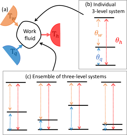
Figure 1: (a) Quantum absorption refrigerators operating with (b) an individual 3-level system as its working fluid, (c) an ensemble of distinct 3-level systems, e.g. of different energy spacing and distinct system-bath coupling parameters. The temperatures of the heat baths are marked by $T_{w}>T_{h}>T_{q}$. The transition between the ground level to the intermediate one, of energy gap $\theta_{q}$ is coupled to the cold bath. The transition between the intermediate level to the top one, of gap $\theta_{w}$, is enacted by the work bath. In a cooling operation, heat absorbed by the three-level system from the cold and work baths is emitted to the hot bath.

IV Model I: Ensemble of absorption refrigerators

Fundamental results on autonomous-continuous thermal machines are often illustrated and examined within simple models for quantum absorption refrigerators Kosloff ; Luis ; MarkRev14 ; recent experiments realized a QAR using trapped ions Poem ; ionE . In a QAR, heat is extracted from a cold ($q$) bath and released into a hot ($h$) bath by absorbing heat from the so-called work ($w$) reservoir. The reversed operation realizes a heat engine. We identify three temperatures, $T_{w}>T_{h}>T_{q}$ in a QAR, and three stochastic heat currents, $w,h,q$, defined positive when flowing towards the system.

The performance of QARs has been investigated in different models for elucidating principles in quantum thermodynamics. For example, QARs have been analyzed from weak to strong couplings to the baths Brandes ; AMu ; HavaNJP ; Tanimura16 , in models supporting multiple competing cycles Correa15 ; HavaM , and when quantum coherences between eigenstates survive in the steady state limit KilgourQAR ; Junjie21 ; these are illustrative examples out of a rich literature. In this paper, we utilize the three-level model of Scovil and Schulz-DuBois Scovil to illustrate bounds on relative fluctuations of currents for an ensemble of QARs. We limit our discussion to the weak system-bath coupling limit, which can be handled with a perturbative quantum Master equation, providing the full counting statistics of the model Segal18 ; Junjie21 .

A schematic diagram of our model is displayed in Fig. 1(a). An individual 3LQAR, illustrated in Fig. 1(b), had particularly served to elucidate concepts in quantum thermodynamics, since at weak system-bath coupling it can be analytically solved. In this model, the three baths are coupled selectively to the different transitions: The cold ($q$) bath allows the transitions across $\theta_{q}$, from the ground state to the intermediate level. The work ($w$) bath is coupled to a transition of energy gap $\theta_{w}$, from the intermediate level to the top one. In a cooling process, the hot bath ($h$) extracts the heat, $\theta_{q}+\theta_{w}$.

IV.1 Single refrigerator, $N=1$

Consider an individual 3LQAR of spacings $\theta_{q}$ and $\theta_{w}$. The cooling efficiency of the engine is defined as $\eta=\frac{\langle q\rangle}{\langle w\rangle}$ with $q$ ($w$) the stochastic cooling (work) heat currents. It can be shown that in the weak system-bath coupling limit, an individual 3LQAR operates in the TC limit: for every quanta $\theta_{q}$ absorbed from $T_{q}$, a quanta $\theta_{w}$ must be absorbed from the work bath. The efficiency and $\eta^{(n)}$ therefore obey the following relations Segal18 ,

$$\eta \equiv \frac{\langle q\rangle}{\langle w\rangle}=\frac{\theta_{q}}{\theta_{w}},\,\,\,\,\,\$$

$$\eta^{(n)} \equiv \frac{\langle\langle q^{n}\rangle\rangle}{\langle\langle w^{n}\rangle\rangle}=\left(\frac{\theta_{q}}{\theta_{w}}\right)^{n}=\eta^{n}\,\,\,\,\,n=2,3,...$$ (14)

Furthermore, the cooling condition is Segal18

$$\langle q\rangle \propto n_{q}(\theta_{q})n_{w}(\theta_{w})[n_{h}(\theta_{h})+1]$$ (15)

$$- [n_{q}(\theta_{q})+1][n_{w}(\theta_{w})+1]n_{h}(\theta_{h})\geq 0,$$

with $n_{i}(\theta_{i})=\frac{1}{e^{\beta_{i}\theta_{i}}-1}$ the Bose Einstein distribution function of the bath $i=h,w,q$ with transition $\theta_{i}$. The cooling condition can be equivalently written as

$$\frac{\theta_{q}}{\theta_{w}}\leq\frac{\beta_{h}-\beta_{w}}{\beta_{q}-\beta_{h}},$$ (16)

with $\beta_{i}=1/T_{i}$ the inverse temperature. We identify the left hand side by the efficiency, $\eta$, and the right hand side by the Carnot efficiency, thus

$$\eta\leq\eta_{C}=\frac{\beta_{h}-\beta_{w}}{\beta_{q}-\beta_{h}}.$$ (17)

Altogether, an individual 3LQAR operates in the TC limit and it satisfies

$$\eta^{n}=\eta^{(n)}\leq\eta_{C}^{n}.$$ (18)

IV.2 Ensemble of $N>1$ distinct refrigerators

An ensemble of distinct uncorrelated refrigerators, with possibly different spacings $\theta_{q}$ and $\theta_{w}$ and different system-bath coupling energies, provides a nontrivial setting for exemplifying the lower bound on ratios of fluctuations. We represent such an ensemble in Fig. 1(c). We assume that all our systems are operating between the same heat baths, $T_{i}$; $i=w,h,q$, and we fix $\theta_{h}$.

First, given the validity of the upper bound, Eq. (18) for each individual machine, we conclude that a similar upper bound holds for the ensemble, as we proved in Sec. II. In what follows we therefore focus on establishing a lower bound on $\eta_{N}^{(n)}$.

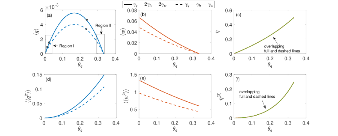
Figure 2: Exemplifying the performance of 3LQARs operating between $\beta_{q}$=0.4, $\beta_{h}$=0.2, and $\beta_{w}$=0.1. (a) Cooling current, (b) current extracted from the work bath, (c) cooling efficiency, (d) fluctuations of cooling current, (e) fluctuations of the so-called work current, and (f) the relative noise $\eta^{(2)}$. Other parameters are $\theta_{h}=1$, and system-bath couplings $\gamma_{q}=\gamma_{h}=\gamma_{w}$ (dashed), $\gamma_{q}=2\gamma_{h}=2\gamma_{w}$ (full). In Sec. IV.2.2, We prove the lower bound $\eta_{N}^{n}\leq\eta_{N}^{(n)}$ in Region I. In Appendix A, it is proved to hold in Region II, albeit only for $n=2$ and $N=2$.

IV.2.1 QARs with different system-bath couplings

We consider an ensemble of three-level systems, each with different coupling strength to the baths but with the same gaps $\theta_{q}$ and $\theta_{w}$. Members of this ensemble sit vertically (at the same $\theta_{q}$) along different curves as exemplified in Fig. 2(a) with asterisks. While the heat currents depend on both the coupling parameters and the energy spacings, notably for any individual refrigerator the ratio $\eta^{(n)}$ depends only on the latter. Next we prove the saturation of the lower bound,

$$\eta_{N}^{n}=\eta_{N}^{(n)}.$$ (19)

For each 3LQAR, $\langle w_{k}\rangle/\langle q_{k}\rangle=\theta_{w}/\theta_{q}\equiv\alpha$, see Eq. (14). Therefore, the efficiency of the ensemble of refrigerators to the power $n$ is

$$\eta_{N}^{n} = \left(\frac{\sum_{k=1}^{N}\langle q_{k}\rangle}{\sum_{k=1}^{N}\langle w_{k}\rangle}\right)^{n}$$ (20)

$$= \left(\sum_{j}\frac{\langle q_{j}\rangle}{\langle w_{j}\rangle}\frac{\langle\omega_{j}\rangle}{\sum_{k}\langle w_{k}\rangle}\right)^{n}=\frac{1}{\alpha^{n}}.$$

Similarly, based on Eq. (14),

$$\eta_{N}^{(n)}=\left(\frac{\sum_{k=1}^{N}{\langle\langle}q_{k}^{n}{\rangle\rangle}}{\sum_{k=1}^{N}{\langle\langle}w_{k}^{n}{\rangle\rangle}}\right)^{n}=\frac{1}{\alpha^{n}},$$ (21)

and we confirm Eq. (19).

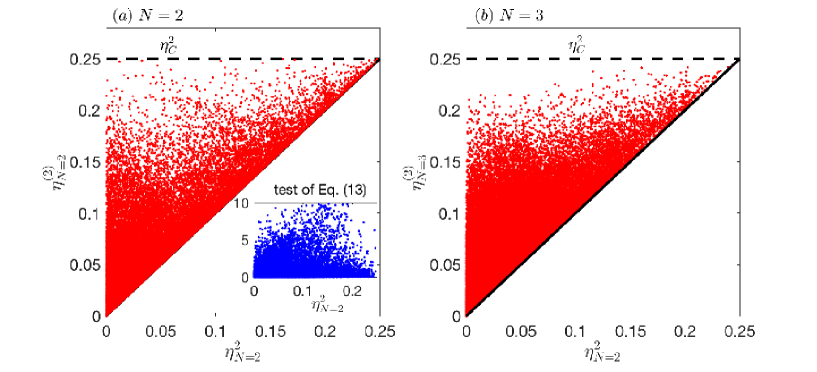
Figure 3: Demonstration that the lower bound $\eta_{N}^{2}\leq\eta^{(2)}_{N}$ is valid beyond Regions I and II of the cooling window. (a) Each dot corresponds to a pair of three-level systems with random values for $\theta_{q}$ and system-bath couplings, $\gamma_{i}$. For this pair, we calculate the total cooling and work currents, as well as their fluctuations. In the inset we test the inequality (13), which is stronger than the lower bound: We present the difference ${\langle\langle}w_{A}^{2}{\rangle\rangle}/{\langle\langle}w_{B}^{2}{\rangle\rangle}-\langle w_{A}\rangle/\langle w_{B}\rangle$ for pairs with $\eta_{A}\geq\eta_{B}$ and show that it is always positive. (b) Same calculations as in (a), but for a triplet of 3LQARs. Temperatures are the same as in Fig. 2. Coupling strengths are uniformly sampled from $0\leq\gamma_{i}\leq 1$, $\theta_{q}$ is sampled from the cooling region.

IV.2.2 QARs with distinct gaps

We now prove the lower bound for an ensemble of 3LQARs characterized by distinct energy gaps, but coupled in the same manner to the different baths; we highlight that each three-level system may couple asymmetrically to the three different baths, but all the three-level systems follow the same coupling parameters. The proof described in this Section holds in the low-cooling regime identified as Region I in Fig. 2(a); points marked by circles exemplify members of this ensemble. In Appendix A we describe a complementary proof (for $N=2$ and $n$=2) that holds in Region II, at the edge of the cooling window marked in Fig. 2(a).

Henceforth, for simplicity and without loss of generality we set the total gap at $\theta_{h}=1$. Assuming that $\theta_{q}\ll 1$, we Taylor-expand the cooling current,

$$\langle q\rangle\approx\alpha\theta_{q}+\beta\theta_{q}^{2}+...$$ (22)

Plugging this expansion into $\eta=\frac{\langle q\rangle}{\langle w\rangle}=\frac{\theta_{q}}{\theta_{w}}$ provides a consistent expansion for the input work,

$$\langle w\rangle\approx\alpha-(\alpha-\beta)\theta_{q}+...$$ (23)

Similarly, we write a Taylor expansion for the fluctuations of the cooling current,

$${\langle\langle}q^{2}{\rangle\rangle}\approx\gamma\theta_{q}^{2}+\delta\theta_{q}^{3}+...$$ (24)

and using $\eta^{(2)}=\frac{\theta_{q}^{2}}{\theta_{w}^{2}}=\frac{{\langle\langle}q^{2}{\rangle\rangle}}{{\langle\langle}w^{2}{\rangle\rangle}}$ put together the consistent expansion for the fluctuations of the work current,

$${\langle\langle}w^{2}{\rangle\rangle}\approx\gamma+\theta_{q}(\delta-2\gamma)+...$$ (25)

Since we assume small cooling current and correspondingly small fluctuations (see Fig. 2), $\theta_{q}\ll 1$, $\beta\theta_{q}\ll\alpha$, and $\delta\theta_{q}\ll\gamma$, the lowest order expansions for the currents and their fluctuations are,

$$\langle q\rangle \approx \alpha\theta_{q},\,\,\,\,\ \langle w\rangle\approx\alpha.$$

$${\langle\langle}q^{2}{\rangle\rangle} \approx \gamma\theta_{q}^{2},\,\,\,\,{\langle\langle}w^{2}{\rangle\rangle}\approx\gamma.$$ (26)

We are now ready to test the lower bound. We begin with two refrigerators A and B of spacings $\theta_{qA}$ and $\theta_{qB}$ that are coupled in the same manner to the baths (for example, A and B are marked by circles in Fig. 2). Since these systems lie on the same curve, $\langle q_{A}\rangle\approx\alpha\theta_{qA}$, $\langle q_{B}\rangle\approx\alpha\theta_{qB}$, $\langle w_{A}\rangle\approx\langle w_{A}\rangle\approx\alpha$. Similarly, ${\langle\langle}q_{A}^{2}{\rangle\rangle}\approx\gamma\theta_{qA}^{2}$, ${\langle\langle}q_{B}^{2}{\rangle\rangle}\approx\gamma\theta_{qB}^{2}$, ${\langle\langle}w_{A}^{2}{\rangle\rangle}\approx{\langle\langle}w_{B}^{2}{\rangle\rangle}\approx\gamma$. We now test the inequality

$$\eta^{2}_{N=2}=\left(\frac{\langle q_{A}\rangle+\langle q_{B}\rangle}{\langle w_{A}\rangle+\langle w_{B}\rangle}\right)^{2}\leq\frac{{\langle\langle}q_{A}^{2}{\rangle\rangle}+{\langle\langle}q_{B}^{2}{\rangle\rangle}}{{\langle\langle}w_{A}^{2}{\rangle\rangle}+{\langle\langle}w_{B}^{2}{\rangle\rangle}}=\eta^{(2)}_{N=2},$$

(27)

by substituting the currents and fluctuations. It reduces to

$$\frac{(\theta_{qA}+\theta_{qB})^{2}}{4}\leq\frac{\theta_{qA}^{2}+\theta_{qB}^{2}}{2},$$ (28)

which is true since $(\theta_{qA}-\theta_{qB})^{2}\geq 0$.

This proof can be generalized to the bound on $\eta^{(n)}$ for an ensemble of $N$ refrigerators. Given the small-$\theta_{q}$ expansions of the $n$th cumulant Segal18 , ${\langle\langle}q^{n}_{k}{\rangle\rangle}\approx\gamma_{n}\theta_{qk}^{n}$, ${\langle\langle}w^{n}_{k}{\rangle\rangle}\approx\gamma_{n}$, the lower-bound inequality reads

$$\eta^{n}_{N}=\left(\frac{\sum_{k}\theta_{qk}}{N}\right)^{n}\leq\frac{\sum_{k}\theta_{qk}^{n}}{N}=\eta^{(n)}_{N}.$$ (29)

Taking the $n$th root gives the desired result by the power mean inequalityineqHandbook , with power 1 on the left hand side and $n$ on the right,

$$\eta_{N}=\left(\frac{1}{N}\sum_{k}\theta_{qk}\right)\leq\left(\frac{1}{N}\sum_{k}\theta_{qk}^{n}\right)^{1/n}=\left[\eta_{N}^{(n)}\right]^{1/n}.$$

(30)

The power mean inequality also implies that $n=2$ provides the tightest bound on $\eta_{N}$.

We note that in general, the assumption of the cooling current being linear in the gap, $\langle q\rangle=\alpha\theta_{q}$, does not necessarily correspond to a linear response limit, $\langle q\rangle\propto(T_{w}-T_{q})$. However, for the 3LQARs, this is in fact the case Segal18 : A linear dependence of $\langle q\rangle$ with $\theta_{q}$ develops hand in hand with the current becoming linear in the temperature difference, though the temperature difference could be large, $\Delta T/T_{i}\gg 1$.

In Appendix A, we prove the lower bound in Region II as marked in Fig. 2, albeit limited to $n=2$ and $N=2$.

IV.2.3 Simulations

We exemplify in Fig. 2 the behavior of individual 3LQARs. The population dynamics, heat currents and their fluctuations are calculated as described in Ref. Segal18 using kinetic-like quantum master equations. The three-level system is coupled to the heat baths with an Ohmic spectral density function, with the excitation rate constant e.g. between the lowest state to the intermediate one, $k_{q}=\Gamma_{q}(\theta_{q})n_{i}(\theta_{q})$ where we use an Ohmic model, $\Gamma_{q}(\theta_{q})=\gamma_{q}\theta_{q}$; $n_{i}(\theta_{i})$ is the Bose-Einstein distribution function. The relaxation rate constant follows from local detailed balance. $\gamma_{i}$ are dimensionless coefficients that control the coupling strength. Simulations in Fig. 2 agree with theoretical results for the efficiency $\eta=\theta_{q}/\theta_{w}$ and the ratio of fluctuations, $\eta^{(2)}=(\theta_{q}/\theta_{w})^{2}$.

In Fig. 3(a), we present simulation results for $\eta^{(2)}_{N}$. We generate a randomized set of 300 refrigerators by sampling uniformly over different values of $\theta_{q}$ within the cooling domain. As for the coupling strength, they are sampled from a uniform distribution $0\leq\gamma_{i}\leq 1$, and they can be distinct and unequal at each realization ($\gamma_{h}\neq\gamma_{q}\neq\gamma_{w}$). We then consider every possible pair of refrigerators and calculate for this pair the total cooling ($\langle q_{A}\rangle+\langle q_{B}\rangle$) and work currents ($\langle w_{A}\rangle+\langle w_{B}\rangle$), as well as their fluctuations, ${\langle\langle}q_{A}^{2}{\rangle\rangle}+{\langle\langle}q_{B}^{2}{\rangle\rangle}$ and ${\langle\langle}w_{A}^{2}{\rangle\rangle}+{\langle\langle}w_{B}^{2}{\rangle\rangle}$. This allows us to calculate the efficiency for each pair, $\eta_{N=2}=(\langle q_{A}\rangle+\langle q_{B}\rangle)/(\langle w_{A}\rangle+\langle w_{B}\rangle)$, and the ratio of their fluctuations, $\eta_{N=2}^{(2)}$. Though most of our refrigerators lie outside Regions I and II, we do not observe violations to the lower bound, $\eta_{N=2}^{2}\leq\eta_{N=2}^{(2)}$; note that parameters are outside the linear-response regime Gerry .

In Fig. 3(b), we select 90,000 samples of triplet 3LQARs and calculate their total current and fluctuations; the total cooling current is $\langle q_{A}\rangle+\langle q_{B}\rangle+\langle q_{C}\rangle$ and the associated fluctuation is ${\langle\langle}q_{A}^{2}{\rangle\rangle}+{\langle\langle}q_{B}^{2}{\rangle\rangle}+{\langle\langle}q_{C}^{2}{\rangle\rangle}$. We then obtain the efficiency for a triplet 3LQAR and the ratio over fluctuations of these machines. Again we confirm based on simulations that the lower bound (9) is satisfied.

IV.2.4 Discussion

We organize our observations up to this point on the validity of the bounds (4) for an ensemble of tight-coupling refrigerators. First, the upper bound holds without additional assumptions (Sec. II). As for a lower bound on $\eta^{(n)}$, for the 3LQARs as discussed in this Sec., we proved that: (ii) The lower bound saturates for an ensemble of systems with identical spacings, $\theta_{q}$, but distinct couplings to the baths. (iii) The lower bound holds for an ensemble of systems operating with equal coupling schemes. This proof hold in the limit of small cooling currents, in Region I, characterized by a vanishing $\theta_{q}$. We were also able to prove (Appendix A) the lower bound in Region II, characterized by a vanishing input work current, albeit limited to $n=2$ and $N=2$. (iv) Extensive simulations confirmed the validity of the lower bound more broadly beyond linear response. Even more so, our simulations showed that an inequality more general than the lower bound holds, namely Eq. (13). (v) In Appendix B we discuss the validity of the lower bound for a three-level model operating as an engine.

V Model II: Ensemble of tight-coupling thermoelectric junctions

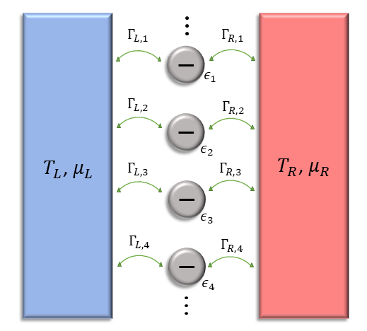
Figure 4: An ensemble of thermoelectric junctions, made of a collection of noninteracting and uncorrelated quantum dots each characterized by a resonant level $\epsilon_{k}$ and coupling strengths $\Gamma_{L,k}$ and $\Gamma_{R,k}$ to the left and right lead, respectively. The junctions all operate between the same metal leads.

A thermoelectric junction comprises a left $(L)$ and right $(R)$ metal lead, between which charge and energy transport may be mediated through an embedded quantum system. The leads serve as thermal baths, differing in temperature and chemical potential such that the associated affinities oppose one anotherbenenti17 ; we suppose that $T_{L}<T_{R}$ and $\mu_{L}>\mu_{R}$. In what follows, we assume resonant electron transport through a discrete level LinkeE , and discuss the existence of the lower bound on $\eta^{(n)}_{N}$ for an ensemble with $N$ thermoelectric junctions as depicted in Fig. 4.

V.1 Single junction, $N=1$

We identify a stochastic charge current $j_{k}$, for a junction labelled by $k$, focusing here on the tight-coupling limit Caplan ; benenti17 , wherein the mean energy current is $\epsilon_{k}\langle j_{k}\rangle$–proportional to the charge current, where $\epsilon_{k}$ is the resonant level of a single quantum dot characterizing the system through which transport is mediated. In this limit, the charge current and fluctuations are given by Levitov ; schonhammer07

$$\langle j_{k}\rangle = \mathcal{T}_{1}\left[f_{L}(\epsilon_{k})-f_{R}(\epsilon_{k})\right],$$

$${\langle\langle}j_{k}^{2}{\rangle\rangle} = \mathcal{T}_{1}\left[f_{L}(\epsilon_{k})(1-f_{R}(\epsilon_{k}))+f_{R}(\epsilon_{k})(1-f_{L}(\epsilon_{k})\right]$$ (31)

$$-\mathcal{T}_{2}\left[f_{L}(\epsilon_{k})-f_{R}(\epsilon_{k})\right]^{2}.$$

The coefficients $\mathcal{T}_{1}$ and $\mathcal{T}_{2}$ are determined by the coupling strengths $\Gamma_{L}$ and $\Gamma_{R}$ between the system and the two leads, $\mathcal{T}_{1}=\frac{\Gamma_{L}\Gamma_{R}}{\Gamma_{L}+\Gamma_{R}}$ and $\mathcal{T}_{2}=\frac{2\Gamma_{L}^{2}\Gamma_{R}^{2}}{(\Gamma_{L}+\Gamma_{R})^{3}}$ for the resonant-level model, see Refs. Bijay-TUR ; Junjie-TUR . $f_{L}(\epsilon)$ and $f_{R}(\epsilon)$ are the Fermi-Dirac distributions for the two leads. A thermoelectric device may act as a refrigerator or an engine in various operational regimes, as determined by the directions of power and heat currents, which are proportional to the charge current in the TC limit. The mean currents thus obey $\langle w_{k}\rangle=\Delta\mu\langle j_{k}\rangle$, $\langle q_{k}\rangle=(\epsilon_{k}-\mu_{\nu})\langle j_{k}\rangle$ ($\nu=L$ for a refrigerator, $R$ for an engine) with $\Delta\mu=\mu_{L}-\mu_{R}$. The fluctuations in these quantities are similarly determined by those for the charge current: ${\langle\langle}w_{k}^{2}{\rangle\rangle}=\Delta\mu^{2}{\langle\langle}j_{k}^{2}{\rangle\rangle}$, ${\langle\langle}q_{k}^{2}{\rangle\rangle}=(\epsilon_{k}-\mu_{\nu})^{2}{\langle\langle}j_{k}^{2}{\rangle\rangle}$.

An individual tight-coupling thermoelectric junction has been shown to satisfy the equality $\eta_{k}^{n}=\eta_{k}^{(n)}$ for any $n=1,2,3,...$Gerry , where, with $\epsilon_{k}$ the dot energy for the machine $k$,

$$\eta_{k} = \frac{\Delta\mu}{\epsilon_{k}-\mu_{R}}\>\textrm{(engine)}$$

$$\eta_{k} = \frac{\epsilon_{k}-\mu_{L}}{\Delta\mu}\>\textrm{(refrigerator)}.$$ (32)

Immediately, the upper bound, $\eta_{k}^{(n)}\leq\eta_{C}^{n}$, also holdsGerry where $\eta_{C}$ represents the operational Carnot bound.

Figure 5: Exemplifying the performance of individual thermoelectric refrigerators between $\beta_{L}$=2, $\beta_{L}$=1, $\mu_{L}=1$, and $\mu_{R}=-1$. (a) Cooling current, (b) work current, (c) cooling efficiency, (d) fluctuations of cooling current and (e) work current, and (f) the relative noise $\eta^{(2)}$. In Sec. V.2.2 we prove the lower bound in Region II under some conditions. Region I is explored in Appendix C.

V.2 Ensemble of distinct thermoelectric junctions

We now consider an ensemble of distinct tight-coupling thermoelectric junctions, labelled by $k$, whose internal parameters such as $\epsilon_{k}$ and system-lead coupling strengths may differ, but which operate between leads with the same set of bath parameters. For example, we envision a thermoelectric device with parallel quantum dots each conducting resonantly with their own energy and coupling strengths to the metal electrode, see Fig. 4.

The validity of the upper bound for a single junction, along with the general result expressed in Eq. (8), leads to the analogous upper bound for an ensemble of such junctions as discussed in Sec. II. The following discussion will therefore focus on when the lower bound, $\eta^{2}\leq\eta^{(n)}$, holds for such an ensemble.

V.2.1 Thermoelectric junctions with different system-bath couplings

Consider an ensemble of $N$ thermoelectric junctions, labelled by $k$, with the same resonant level, $\epsilon$, characterizing the quantum system, as represented in Fig. 5(a) by the pair of asterisks. The cooling efficiency, $\langle q_{k}\rangle/\langle w_{k}\rangle=(\epsilon-\mu_{L})/\Delta\mu$ is equal for all such refrigerators since it does not depend on the system-bath coupling. As such, one can readily prove, via an argument mirroring that in Section IV.2.1, the strict equality $\eta_{N}^{n}=\eta_{N}^{(n)}$ for the ensemble.

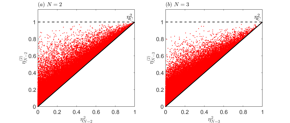
Figure 6: Demonstration that the lower bound $\eta_{N}^{2}\leq\eta^{(2)}_{N}$ is valid beyond the linear regime of the charge current. (a) Each dot corresponds to a pair of tight-coupling thermoelectric refrigerators with random values for $\epsilon_{k}$ as well as coupling strengths. For this pair, we calculate the total cooling and work currents as well as their fluctuations. (b) Same calculations as in (a), but for a triplet of thermoelectrics. $\beta_{L}=2$, $\beta_{R}=1$, $\mu_{L}=1$, and $\mu_{R}=-1$. Coupling strengths are uniformly sampled from $0\leq\Gamma_{i}\leq 1/2$, $\epsilon_{k}$ is sampled from the cooling region, $1<\epsilon_{k}<3$. The operational Carnot bound for refrigeration is $\eta_{C}=\beta_{R}/(\beta_{L}-\beta_{R})$.

V.2.2 Thermoelectric junctions with distinct energy levels

Now, we will focus specifically on the case of a pair ($N=2$) of tight-coupling thermoelectric junctions, $A$ and $B$, operating as refrigerators, with cooling currents flowing from the left (cold) lead, $\langle q_{k}\rangle=(\epsilon_{k}-\mu_{L})\langle j_{k}\rangle$, $k=A,B$. The cooling and work currents are taken, by convention, to be positive. We will show that for this pair taken as a single device, the lower bound, $\eta_{N=2}^{2}\leq\eta_{N=2}^{(2)}$ holds, provided we restrict ourselves to a specific range of values for $\epsilon_{A}$ and $\epsilon_{B}$, namely, Region II, near the edge of the cooling window such that $\langle j_{k}\rangle$ is small. For instance, such an ensemble may be represented by the pair of circles in Fig. 5(a). Furthermore, we will suppose that one refrigerator, say $B$, has a significantly larger charge current than the other ($\langle j_{A}\rangle/\langle j_{B}\rangle\ll 1$). This requires that $\epsilon_{A}>\epsilon_{B}$, so $\eta_{A}>\eta_{B}$. The complementary proof for Region I is given in Appendix C.

We express the dot energy for each thermoelectric refrigerator as $\epsilon_{k}=\mu_{R}+\Delta\mu\beta_{L}/\Delta\beta-u_{k}$ with $\Delta\beta=\beta_{L}-\beta_{R}$, $\Delta\mu=\mu_{L}-\mu_{R}$. Note that the charge current vanishes when $u_{k}=0$ Linke05 , and initially grows linearly with $u_{k}$: $\langle j_{k}\rangle\approx\alpha u_{k}$, where $\alpha$ is some constant coefficient. Then we have that $u_{A}/u_{B}\ll 1$, and we may write out the full efficiency of the pair, $\eta_{N=2}=[(\epsilon_{A}-\mu_{L})u_{A}+(\epsilon_{B}-\mu_{L})u_{B}]/[(u_{A}+u_{B})\Delta\mu]$. Truncating after first order in this ratio, and squaring, we get,

$$\eta_{N=2}^{2}\approx\eta_{B}^{(2)}\left[1+2\bigg{(}\frac{\epsilon_{A}-\mu_{L}}{\epsilon_{B}-\mu_{L}}-1\bigg{)}\frac{u_{A}}{u_{B}}\right].$$ (33)

The assumption of small charge current permits the approximation that fluctuations are predominantly due to single-electron processeses; we refer to Eq. (V.1) and ignore the contribution proportional to $(f_{L}(\epsilon_{k})-f_{R}(\epsilon_{k}))^{2}$, writing

$${\langle\langle}j_{k}^{2}{\rangle\rangle}=\mathcal{T}_{1}\left[f_{L}(\epsilon_{k})(1-f_{R}(\epsilon_{k}))+f_{R}(\epsilon_{k})(1-f_{L}(\epsilon_{k}))\right].$$ (34)

Thus can be shown to be proportional to the charge current,

$${\langle\langle}j_{k}^{2}{\rangle\rangle}=\langle j_{k}\rangle\coth\left(\frac{\Delta\beta u_{k}}{2}\right)\equiv c_{k}\langle j_{k}\rangle,$$ (35)

with $c_{k}$ defined from this relation. The ratio of fluctuations of the cooling current to work current is given in terms of $u_{A}$ and $u_{B}$ as

$$\eta_{N=2}^{(2)}=\eta_{B}^{(2)}\frac{1+\frac{(\epsilon_{A}-\mu_{L})^{2}}{(\epsilon_{B}-\mu_{L})^{2}}\frac{c_{A}u_{A}}{c_{B}u_{B}}}{1+\frac{c_{A}u_{A}}{c_{B}u_{B}}}.$$ (36)

As $u_{k}$ approaches zero, $c_{k}$ goes to infinity, so we cannot assume $c_{A}u_{A}/c_{B}u_{B}$ is small. However, we can still compare $\eta_{N=2}^{2}$ and $\eta_{N=2}^{(2)}$, finding, after keeping only terms up to first order in $u_{A}/u_{B}$, that the lower bound is equivalent to the inequality

$$2\bigg{(}\frac{\epsilon_{A}-\mu_{L}}{\epsilon_{B}-\mu_{L}}-1\bigg{)}\leq\frac{c_{A}}{c_{B}}\left[\frac{(\epsilon_{A}-\mu_{L})^{2}}{(\epsilon_{B}-\mu_{L})^{2}}-1\right].$$ (37)

Since $\epsilon_{A}>\epsilon_{B}$, this holds as long as $c_{A}/c_{B}\geq 2$. We note that this is certainly the case since, by assumption, $u_{A}$ and $u_{B}$ are small, so $c_{A}/c_{B}\approx u_{B}/u_{A}\gg 1$. We may conclude that in this regime, $\eta_{N=2}^{2}\leq\eta_{N=2}^{(2)}$.

The proof outlined in this section is quite limited: It holds for a pair of refrigerators and only for the second cumulant, $n=2$. Complementing this proof, in Appendix C, we prove the lower bound in Region I, now for an ensemble of arbitrary size $N$ and to the order $n$. Furthermore, Fig. 6 demonstrates, via the results of simulations, that the upper and lower bounds (for $n=2$) appear to hold for pairs and triplets of thermoelectric junctions outside Regions I and II.

Altogether, we proved the validity of the lower bound for three-level refrigerators and thermoelectric refrigerators in corresponding cases, in Region I and II. In Appendix D, we consider an analogous set of assumptions as discussed in this subsection, but applied to thermoelectric junctions operating as engines. We find in this case that the lower bound must be violated.

VI Summary

We studied universal bounds on ratios of fluctuations, as well as higher order cumulants, in an ensemble of distinct, uncorrelated thermal machines operating in steady state and arbitrarily far from equilibrium. We built our bounds for the ensemble of machines from bounds on the individual machine, $\eta_{k}^{n}=\eta_{k}^{(n)}\leq\eta_{C}^{n}$. These relations hold e.g., for systems obeying the tight coupling limit, such as three-level absorption refrigerators and resonant-level thermoelectric junctions. $\eta_{C}$ is the Carnot efficiency and $\eta^{(n)}$ is ratio of the $n$th cumulants of the output current to input current. We proved that:

(i) An upper bound holds for an ensemble of $N$ distinct machines, engines or refrigerators, arbitrarily far from equilibrium, $\eta_{N}^{(n)}\leq\eta_{C}^{n}$.

(ii) The lower bound on the ensemble, $\eta_{N}^{n}\leq\eta_{N}^{(n)}$, is more limited in scope. While it seems to hold for refrigerators, based on analytic and numerical work, we demonstrated that thermoelectric engines may violate the lower bound for $N\geq 2$.

(iii) Focusing on three-level quantum absorption refrigerators and thermoelectric junctions, we proved the validity of the lower bound, $\eta_{N}^{n}\leq\eta_{N}^{(n)}$, in different cases: when the cooling current was small, and for an ensemble of distinct machines with identical efficiencies.

(iv) While analytic proofs of the lower bound for refrigerators were limited in scope (e.g. to $n=2$ and $N=2$ in Region II near the edge of the cooling window), simulations beyond these strict regimes support its validity more broadly.

The significance of our study is in developing bounds for ensemble of machines. While bounds on the individual system may be trivial, as in the tight coupling limit, a machine that collects input and output from several tightly-coupled components (recall Figs. 1 and 4) may behave nontrivially in this respect, even under classical laws and in the absence of interactions between components. Adding interactions to the working fluid e.g. Coulomb interactions between quantum dots in a themroelectic device or by using an interacting atomic gas, opens up the door to new effects, such as many-particle enhancement of performance delCampoEnt16 ; delCampoNJP16 ; delCampoNPJ19 ; Reimann ; Gernot19 ; Gernot . Furthermore, quantum statistical effects combined with interactions or collective unitary operations on the components can further enhance performance, as predicted in Ref. delCampo .

An important result of our work is in tightening bounds on efficiency: As an outcome of the lower bound, Eq. (30), one immediately finds that $\eta\leq\left[\eta^{(n)}\right]^{1/n}\leq\eta_{C}$, and that the case with $n=2$ provides the tightest lower bound. Whether this is a general result, or only valid for refrigerators in the small-$\theta$ small-cooling domain remains an open question.

In future work we will focus on understanding the validity of the lower bound on $\eta^{(n)}$ in general settings, and on exploring the fundamental differences between engines and refrigerators as pertain to bounds on fluctuations.

Appendix A: Lower bound on $\eta_{2}^{(2)}$ for 3LQARs at the boundary of the cooling region (Region II)

Here, we present a proof of the validity of a lower bound for two 3LQARs, applicable in the limit of small currents. This proof holds at the boundary of the cooling domain (see Region II in Fig. 2). The proof presented here is limited to two QARs, and its extensions to $N$ refrigerators is not obvious.

For simplicity, we define the scaled currents $q/\theta_{q}\to q$ and $w/\theta_{w}\to w$. We also assume that $T_{w}\to\infty$. The cooling current and its noise are given in terms of the bath-induced transition rate constants $\Gamma_{q,h,w}$, see text in Sec. IV.2.3 and Ref. Segal18 . We also use the short notation $\tilde{\Gamma}_{i}=\Gamma_{i}(\theta_{i})n_{i}(\theta_{i})$. The cooling current and its fluctuations are given by Segal18

$$\langle q\rangle=\frac{\tilde{\Gamma}_{h}\tilde{\Gamma}_{q}\tilde{\Gamma}_{w}\left(e^{\theta_{h}/T_{h}}-e^{\theta_{q}/T_{q}}\right)}{M},$$ (A1)

$${\langle\langle}q^{2}{\rangle\rangle}=\frac{2\left(\tilde{\Gamma}_{h}+\tilde{\Gamma}_{q}+\tilde{\Gamma}_{w}+\tilde{\Gamma}_{q}e^{\theta_{q}/T_{q}}+\tilde{\Gamma}_{w}+\tilde{\Gamma}_{h}e^{\theta_{h}/T_{h}}\right)\langle q\rangle^{2}}{M}+\frac{\tilde{\Gamma}_{q}\tilde{\Gamma}_{h}\tilde{\Gamma}_{w}\left(e^{\theta_{h}/T_{h}}+e^{\theta_{q}/T_{q}}\right)}{M}$$

$$\text{with }M=\left(\tilde{\Gamma}_{c}e^{\theta_{q}/T_{q}}+\tilde{\Gamma}_{w}\right)\left(\tilde{\Gamma}_{w}+\tilde{\Gamma}_{q}e^{\theta_{h}/T_{h}}\right)+\left(\tilde{\Gamma}_{q}+\tilde{\Gamma}_{h}\right)\left(\tilde{\Gamma}_{w}+\tilde{\Gamma}_{h}e^{\theta_{q}/T_{q}}\right)+$$

$$\left(\tilde{\Gamma}_{q}+\tilde{\Gamma}_{h}\right)\left(\tilde{\Gamma}_{q}e^{\theta_{q}/T_{q}}+\tilde{\Gamma}_{w}\right)-\tilde{\Gamma}_{q}^{2}e^{\theta_{q}/T_{q}}-\tilde{\Gamma}_{w}^{2}-\tilde{\Gamma}_{h}^{2}e^{\theta_{h}/T_{h}}$$ (A2)

The cooling window is defined by the condition $0<\theta_{q}<\theta_{h}\frac{T_{q}}{T_{h}}$. When $\langle q\rangle\ll\Pi_{i=h,q,w}\tilde{\Gamma}_{i}$, the second term in the noise dominates, thus it is given by

$${\langle\langle}q^{2}{\rangle\rangle}\approx\left|\frac{e^{\theta_{h}/T_{h}}+e^{\theta_{q}/T_{q}}}{e^{\theta_{h}/T_{h}}-e^{\theta_{q}/T_{q}}}\right|\langle q\rangle=\left|\coth\left(\frac{\theta_{h}}{2T_{h}}-\frac{\theta_{q}}{2T_{q}}\right)\right|\langle q\rangle\equiv F(\theta_{q})\langle q\rangle$$ (A3)

We now consider two refrigerators, A and B, with identical total gaps $\theta_{h}$, but different internal energies, $\theta_{q_{A}}\neq\theta_{q_{B}}$. Correspondingly, each QAR supports the cooling current $\langle q_{k}\rangle$ with the associated noise ${\langle\langle}q_{k}^{2}{\rangle\rangle}$. As for the lower bound, we would like to show that (recovering the energy gaps in the expressions for the currents and noises):

$$\eta^{2}=\frac{(\theta_{q_{A}}\langle q_{A}\rangle+\theta_{q_{B}}\langle q_{B}\rangle)^{2}}{(\theta_{w_{A}}\langle q_{A}\rangle+\theta_{w_{B}}\langle q_{B}\rangle)^{2}}\leq\frac{\theta^{2}_{q_{A}}{\langle\langle}q_{A}^{2}{\rangle\rangle}+\theta^{2}_{q_{B}}{\langle\langle}q_{B}^{2}{\rangle\rangle}}{\theta^{2}_{w_{A}}{\langle\langle}q_{A}^{2}{\rangle\rangle}+\theta^{2}_{w_{B}}{\langle\langle}q_{B}^{2}{\rangle\rangle}}=\eta^{(2)}$$ (A4)

Using Eq. (A3) and that $\theta_{w}=\theta_{h}-\theta_{q}$, we get

$$\frac{[\theta_{q_{A}}\langle q_{A}\rangle+\theta_{q_{B}}\langle q_{B}\rangle]^{2}}{[(\theta_{h}-\theta_{q_{A}})\langle q_{A}\rangle+(\theta_{h}-\theta_{q_{B}})\langle q_{B}\rangle]^{2}}\leq\frac{\theta^{2}_{q_{A}}F(\theta_{q_{A}})\langle q_{A}\rangle+\theta^{2}_{q_{B}}F(\theta_{q_{B}})\langle q_{B}\rangle}{(\theta_{h}-\theta_{q_{A}})^{2}F(\theta_{q_{A}})\langle q_{A}\rangle+(\theta_{h}-\theta_{q_{B}})^{2}F(\theta_{q_{B}})\langle q_{B}\rangle}.$$ (A5)

After cross-multiplying, all the $\langle q\rangle^{2}$ terms vanish and we are left with

$$\sum_{i\neq k}\left(\theta^{2}_{q_{i}}(\theta_{h}-\theta_{q_{k}})^{2}F(\theta_{q_{k}})+2\theta_{q_{i}}\theta_{q_{k}}(\theta_{h}-\theta_{q_{i}})^{2}F(\theta_{q_{i}})\right)\langle q_{i}\rangle$$ (A6)

$$\leq\sum_{i\neq k}\left(\theta^{2}_{q_{k}}(\theta_{h}-\theta_{q_{i}})^{2}F(\theta_{q_{k}})+2\theta_{q_{i}}^{2}(\theta_{h}-\theta_{q_{i}})(\theta_{h}-\theta_{q_{k}})F(\theta_{q_{i}})\right)\langle q_{i}\rangle$$

Since each current $\langle q\rangle$ can be set freely by setting the transition rates, the inequality is true if and only if each $\langle q\rangle$ part obeys the inequality:

$$\theta^{2}_{q_{A}}(\theta_{h}-\theta_{q_{B}})^{2}F(\theta_{q_{B}})+2\theta_{q_{A}}\theta_{q_{B}}(\theta_{h}-\theta_{q_{A}})^{2}F(\theta_{q_{A}})\leq\theta^{2}_{q_{B}}(\theta_{h}-\theta_{q_{A}})^{2}F(\theta_{q_{B}})+2\theta_{q_{A}}^{2}(\theta_{h}-\theta_{q_{A}})(\theta_{h}-\theta_{q_{B}})F(\theta_{q_{A}}).$$

(A7)

After additional manipulations we get

$$\left[\theta_{h}^{2}\left(\theta_{q_{A}}^{2}-\theta_{q_{B}}^{2}\right)-2\theta_{h}\theta_{q_{A}}\theta_{q_{B}}(\theta_{q_{A}}-\theta_{q_{B}})\right]F(\theta_{q_{B}})+\left[2\theta_{q_{A}}\theta_{h}(\theta_{h}-\theta_{q_{A}})(\theta_{q_{B}}-\theta_{q_{A}})\right]F(\theta_{q_{A}})\leq 0$$

The function $F(\theta)$ is positive, and it grows exponentially as $\theta$ approaches the asymptote at the edge of the cooling window, $\theta_{q}=\theta_{h}\frac{T_{q}}{T_{h}}$, from below. Therefore, if $\theta_{q_{A}}<\theta_{q_{B}}<\theta_{h}\frac{T_{q}}{T_{h}}$, the first term in Eq. (Appendix A: Lower bound on $\eta_{2}^{(2)}$ for 3LQARs at the boundary of the cooling region (Region II)) dominates. It is given by

$$\theta_{h}(\theta_{q_{A}}+\theta_{q_{B}})(\theta_{q_{A}}-\theta_{q_{B}})-2\theta_{q_{A}}\theta_{q_{B}}(\theta_{q_{A}}-\theta_{q_{B}}) \leq 0,$$ (A9)

which is reduced to

$$\theta_{h}(\theta_{q_{A}}+\theta_{q_{B}})-2\theta_{q_{A}}\theta_{q_{B}} \geq 0.$$ (A10)

This is true since $\theta_{h}>\theta_{qA}$ and $\theta_{h}>\theta_{qB}$.

Likewise, the second term in Eq. (Appendix A: Lower bound on $\eta_{2}^{(2)}$ for 3LQARs at the boundary of the cooling region (Region II)) dominates in the opposite case, if $\theta_{q_{B}}<\theta_{q_{A}}<\theta_{h}\frac{T_{q}}{T_{h}}$. We then check whether

$$2\theta_{q_{A}}\theta_{h}(\theta_{h}-\theta_{q_{A}})(\theta_{q_{B}}-\theta_{q_{A}})\leq 0,$$ (A11)

which is true, since the last term is negative and the rest are positive.

Appendix B: Lower bound on $\eta_{2}^{(2)}$ for three-level engines

We consider here the performance of the three-level model as an engine, rather than a refrigerator. We show that in the limit of small currents, at the edge of the engine’s window, the lower bound for $\eta^{(2)}$ holds. This is to be contrasted with behavior observed for a thermoelectic engine, Appendix D, which shows violations to the lower bound in a corresponding domain.

The system acts as an engine when $\theta_{h}\frac{T_{q}}{T_{h}}<\theta_{q}<\theta_{h}$. Heat is absorbed from the hot ($h$) bath and emitted at the $w$ bath as useful work, with leftout heat released at the $q$ bath. In this engine’s regime, assuming the thermal noise dominates (since the current is small), we write

$${\langle\langle}q^{2}{\rangle\rangle}=-F(\theta_{q})\langle q\rangle.$$ (B1)

Recall that by our conventions, $\langle q\rangle$ is positive when flowing into the system, and thus it is negative when the system acts as an engine. Furthermore, when the system operates as an engine, $F$ is positive and decreasing with $\theta_{q}$.

For an engine, the efficiency is the work current over the heat input from the hot bath. As usual, we set the total gap size $\theta_{h}$ the same for both systems. Rewriting Eq. (A4) for the two engines gives

$$\eta^{2}=\frac{(\theta_{w_{A}}\langle q_{A}\rangle+\theta_{w_{B}}\langle q_{B}\rangle)^{2}}{(\theta_{h_{A}}\langle q_{A}\rangle+\theta_{h_{B}}\langle q_{B}\rangle)^{2}}\leq\frac{\theta^{2}_{w_{A}}{\langle\langle}q_{A}^{2}{\rangle\rangle}+\theta^{2}_{w_{B}}{\langle\langle}q_{B}^{2}{\rangle\rangle}}{\theta^{2}_{h_{A}}{\langle\langle}q_{A}^{2}{\rangle\rangle}+\theta^{2}_{h_{B}}{\langle\langle}q_{B}^{2}{\rangle\rangle}}=\eta^{(2)}.$$ (B2)

Recall that $\langle q\rangle$ is a scaled measure, i.e., it counts the number of quanta exchanged, rather than the heat current itself. Following the same steps as in Appendix A, we end with Eq. (A7), but with $\theta_{q}\to\theta_{w}$, except in the $F$ functions, and $\theta_{w}\to\theta_{h}$. As before, we chose without loss of generality only the $\langle q_{A}\rangle$ terms. The lower bound is true if

$$2(\theta_{q_{A}}-\theta_{q_{B}})(\theta_{h}-\theta_{q_{A}})F(\theta_{q_{A}})\leq(\theta_{q_{A}}-\theta_{q_{B}})(2\theta_{h}-\theta_{q_{A}}-\theta_{q_{B}})F(\theta_{q_{B}}).$$ (B3)

When $\theta_{q_{A}}>\theta_{q_{B}}$,

$$2(\theta_{h}-\theta_{q_{A}})F(\theta_{q_{A}})\leq(2\theta_{h}-\theta_{q_{A}}-\theta_{q_{B}})F(\theta_{q_{B}})$$ (B4)

which is true, using that $F$ is a decreasing function of $\theta_{q}$. When $\theta_{q_{A}}<\theta_{q_{B}}$,

$$2(\theta_{h}-\theta_{q_{A}})F(\theta_{q_{A}})\geq(2\theta_{h}-\theta_{q_{A}}-\theta_{q_{B}})F(\theta_{q_{B}}),$$ (B5)

which also holds.

In Fig. 7, we search numerically for violations of the lower bound for an ensemble of three-level absorption engines, in a broad parameter space. As we are not able to identify such violations, we hypothesize that the three-level system acting as either a refrigerator or an engine satisfies the lower bound on $\eta_{N}^{(2)}$.

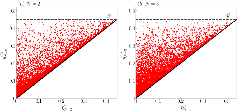
Figure 7: Demonstration that the lower bound $\eta_{N}^{2}\leq\eta^{(2)}_{N}$ is valid for the three-level absorption engine. (a) Each dot corresponds to a pair of engines with random values for $\theta_{q}$ as well as coupling energies. For this pair, we calculate the total work and absorbed heat currents as well as their fluctuations. (b) Same calculations as in (a), but for a triplet of engines. We used $\beta_{q}=0.4$, $\beta_{h}=0.2$, and $\beta_{w}=0.1$. The system-bath coupling strengths are uniformly sampled from $0\leq\gamma_{i}\leq 1$, $\theta_{q}$ is sampled from the engine region.

Appendix C: Lower bound on $\eta_{N}^{(n)}$ for thermoelectric refrigerators in region I

We now turn our attention to a pair of tight-coupling thermoelectric refrigerators, $A$ and $B$, with both $\epsilon_{A}$ and $\epsilon_{B}$ at the opposite end of the cooling window from those discussed in Section V. We refer to this as “Region I”, as depicted in Fig. 5. In this region, $\langle q_{k}\rangle$, $k=A,B$, is small, vanishing when $\epsilon_{k}=\mu_{L}$, however, the charge current itself $\langle j_{k}\rangle$ remains finite and nonzero. We suppose that $\langle j_{A}\rangle\approx\langle j_{B}\rangle\approx\langle j_{m}\rangle|_{\epsilon_{m}=\mu_{L}}\equiv J$. Defining $u_{k}\equiv\epsilon_{k}-\mu_{L}$, we have that $\langle q_{k}\rangle=\langle j_{k}\rangle u_{k}\approx Ju_{k}$. The cooling efficiency of a single refrigerator is $\eta_{k}=u_{k}/\Delta\mu$, and the tight-coupling limit gives $\eta^{(2)}_{k}=(u_{k}/\Delta\mu)^{2}$.

Writing out the efficiency of the pair, we have

$$\eta_{N=2}\approx\frac{\langle q_{A}\rangle+\langle q_{B}\rangle}{2\Delta\mu J}\approx\frac{u_{A}+u_{B}}{2\Delta\mu}=\frac{\eta_{A}}{2}\bigg{(}1+\frac{u_{B}}{u_{A}}\bigg{)}.$$ (C1)

Since Region I is not characterized by a small charge current, we cannot assume that the fluctuations in the charge or heat currents are given predominantly by thermal noise. However, we may echo our assumption above by supposing that ${\langle\langle}j_{A}^{2}{\rangle\rangle}\approx{\langle\langle}j_{B}^{2}{\rangle\rangle}\approx{\langle\langle}j_{m}^{2}{\rangle\rangle}|_{\epsilon_{m}=\mu_{L}}\equiv S$. Then, fluctuations in the cooling currents are given by ${\langle\langle}q_{k}^{2}{\rangle\rangle}\approx Su_{k}^{2}$, and the ratio of cooling to work current fluctuations is given by

$$\eta^{(2)}_{N=2}\approx\frac{u_{A}^{2}+u_{B}^{2}}{2\Delta\mu^{2}}=\frac{\eta_{A}^{(2)}}{2}\left[1+\left(\frac{u_{B}}{u_{A}}\right)^{2}\right].$$ (C2)

In Fig. 8 we demonstrate that Eqs. (C1) and (C2) indeed provide a good approximation for the efficiency and the ratio of fluctuations for refrigerators in Region I.

Squaring Eq. (C1), utilizing that $\eta_{A}^{2}=\eta_{A}^{(2)}$, and comparing it to Eq. (C2), we see that the lower bound, $\eta_{N=2}^{2}\leq\eta_{N=2}^{(2)}$, is equivalent to the inequality

$$\frac{1}{4}\bigg{(}1+\frac{u_{B}}{u_{A}}\bigg{)}^{2}\leq\frac{1}{2}\left[1+\bigg{(}\frac{u_{B}}{u_{A}}\bigg{)}^{2}\right],$$ (C3)

or, rearranging,

$$\bigg{(}\frac{u_{B}}{u_{A}}-1\bigg{)}^{2}\geq 0.$$ (C4)

This is clearly satisfied for any choice of $u_{A}$ and $u_{B}$, so we conclude that the lower bound $\eta_{N=2}^{2}\leq\eta_{N=2}^{(2)}$ is satisfied for a pair of refrigerators in this regime.

We now extend this argument more generally to $n>2$ and $N>2$, by getting expressions for $\eta_{N}$ and $\eta_{N}^{(n)}$ of the ensemble analogous to Eqs. (C1) and (C2),

$$\eta_{N} = \frac{\sum_{k=1}^{N}u_{k}}{N\Delta\mu},$$

$$\eta_{N}^{(n)} = \frac{\sum_{k=1}^{N}u_{k}^{n}}{N\Delta\mu^{n}}.$$ (C5)

Taking the $n^{th}$ root of $\eta_{N}^{(n)}$, we see that the lower bound, $\eta_{N}^{n}\leq\eta_{N}^{(n)}$, is equivalent to

$$\frac{1}{N}\sum_{k=1}^{N}u_{k}\leq\bigg{(}\frac{1}{N}\sum_{k=1}^{N}u_{k}^{n}\bigg{)}^{\frac{1}{n}},$$ (C6)

which is always true as a result of the power mean inequalityineqHandbook .

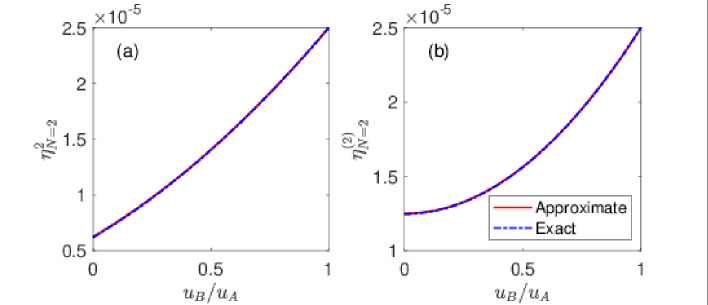
Figure 8: Comparison of the approximate expressions for (a) $\eta_{N=2}^{2}$ and (b) $\eta_{N=2}^{(2)}$, given by Eqs. (C1) and (C2), respectively, with their exact values. We focus on the case $u_{B}<u_{A}$ to avoid redundancy. The good correspondence between approximate and exact values suggests that the approximations made are valid. Indeed, the lower bound is seen to be satisfied. $\beta_{L}=2$, $\beta_{R}=1$, $\mu_{L}=1$, $\mu_{R}=-1$, $u_{A}=0.01$, and $\Gamma_{L}=\Gamma_{R}=1$.

Appendix D: Violation of the lower bound on $\eta_{N=2}^{(2)}$ for a pair of thermoelectric engines

We consider here a pair of thermoelectric engines in the tight-coupling limit, far from equilibrium, operating in the regime of high $\epsilon_{k}$, for both $k=A,B$, and thus small charge current. Note that, due to the assumption of tight-coupling, this operational regime has no upper boundary with respect to $\epsilon_{k}$. Furthermore, we suppose that the magnitude of the charge current is considerably greater for engine $A$ than for $B$. Since, in this regime, charge current decreases with $\epsilon_{k}$, $\epsilon_{B}>\epsilon_{A}$, and thus, $\eta_{A}>\eta_{B}$. We will show that, under these assumptions, the lower bound on the ratio of fluctuations, $\eta_{N=2}^{2}\leq\eta_{N=2}^{(2)}$, must be violated.

In contrast to the refrigerator case, we now define the heat current with respect to the right (hot) lead–$\langle q_{k}\rangle=(\epsilon_{k}-\mu_{R})\langle j_{k}\rangle$. We first write out the efficiency of the pair of engines,

$$\eta_{N=2}=\frac{\langle w\rangle}{\langle q\rangle}=\frac{\Delta\mu(\langle j_{A}\rangle+\langle j_{B}\rangle)}{(\epsilon_{A}-\mu_{R})\langle j_{A}\rangle+(\epsilon_{B}-\mu_{R})\langle j_{B}\rangle}=\eta_{A}\frac{1+\frac{\langle j_{B}\rangle}{\langle j_{A}\rangle}}{1+\frac{\epsilon_{B}-\mu_{R}}{\epsilon_{A}-\mu_{R}}\frac{\langle j_{B}\rangle}{\langle j_{A}\rangle}}.$$ (D1)

Noting that $\langle j_{B}\rangle/\langle j_{A}\rangle\ll 1$, we expand to first order in this ratio. After squaring, we have

$$\eta_{N=2}^{2}\approx\eta_{A}^{2}\left[1+2\bigg{(}1-\frac{\epsilon_{B}-\mu_{R}}{\epsilon_{A}-\mu_{R}}\bigg{)}\frac{\langle j_{B}\rangle}{\langle j_{A}\rangle}\right]=\eta_{A}^{(2)}\left[1+2\bigg{(}1-\frac{\epsilon_{B}-\mu_{R}}{\epsilon_{A}-\mu_{R}}\bigg{)}\frac{\langle j_{B}\rangle}{\langle j_{A}\rangle}\right].$$ (D2)

Next, we consider the fluctuations in the work and heat currents. The assumption of small currents allows us to neglect cotunneling processes, that is contributions proportional to $(f_{L}(\epsilon_{k})-f_{R}(\epsilon_{k}))^{2}$. Furthermore, we use the identity $f_{L}(\epsilon_{k})\left[1-f_{R}(\epsilon_{k})\right]+f_{R}(\epsilon_{k})\left[1-f_{L}(\epsilon_{k})\right]=[f_{L}(\epsilon_{k})-f_{R}(\epsilon_{k})]\coth[(-\Delta\beta\epsilon_{k}+\bar{\beta}\Delta\mu)/2]\equiv c_{k}[f_{L}(\epsilon_{k})-f_{R}(\epsilon_{k})]$ (note that $\Delta\beta=\beta_{L}-\beta_{R}<0$, $\bar{\beta}=(\beta_{L}+\beta_{R})/2$) to express the charge current fluctuations for each engine in terms of the charge current itself,

$${\langle\langle}j_{k}^{2}{\rangle\rangle}=c_{k}\langle j_{k}\rangle.$$ (D3)

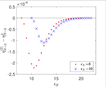
Figure 9: Violations of the lower bound observed for pairs of tight-coupling thermoelectric engines with sufficiently high $\epsilon_{A}$ and $\epsilon_{B}$, shown as a function of $\epsilon_{B}>\epsilon_{A}$ for two choices of $\epsilon_{A}$. Parameters are $\beta_{L}=2$, $\beta_{R}=1$, $\mu_{L}=1$, $\mu_{R}=-1$, and $\Gamma_{L}=\Gamma_{R}=1$.

Then, the ratio of fluctuations for the pair is given by

$$\eta_{N=2}^{(2)}=\frac{{\langle\langle}w^{2}{\rangle\rangle}}{{\langle\langle}q^{2}{\rangle\rangle}}=\frac{\Delta\mu^{2}\left(c_{A}\langle j_{A}\rangle+c_{B}\langle j_{B}\rangle\right)}{(\epsilon_{A}-\mu_{R})^{2}c_{A}\langle j_{A}\rangle+(\epsilon_{B}-\mu_{R})^{2}c_{B}\langle j_{B}\rangle}=\eta_{A}^{(2)}\frac{1+\frac{c_{B}\langle j_{B}\rangle}{c_{A}\langle j_{A}\rangle}}{1+\frac{(\epsilon_{B}-\mu_{R})^{2}c_{B}\langle j_{B}\rangle}{(\epsilon_{A}-\mu_{R})^{2}c_{A}\langle j_{A}\rangle}}.$$ (D4)

In the engine regime, $\epsilon_{B}>\epsilon_{A}$ implies that $|c_{B}|<|c_{A}|$, so we do not have to worry that $c_{B}/c_{A}$ blows up and we may expand Eq. (D4) to first order in $\langle j_{B}\rangle/\langle j_{A}\rangle$, giving

$$\eta_{N=2}^{(2)}\approx\eta_{A}^{(2)}\left[1+\bigg{(}1-\bigg{(}\frac{\epsilon_{B}-\mu_{R}}{\epsilon_{A}-\mu_{R}}\bigg{)}^{2}\bigg{)}\frac{c_{B}\langle j_{B}\rangle}{c_{A}\langle j_{A}\rangle}\right].$$ (D5)

Now, comparing Eqs. (D2) and (D5), we find that the lower bound $\eta_{N=2}^{2}\leq\eta_{N=2}^{(2)}$ is equivalent to the inequality

$$2\bigg{(}1-\frac{\epsilon_{B}-\mu_{R}}{\epsilon_{A}-\mu_{R}}\bigg{)}\leq\frac{c_{B}}{c_{A}}\left[1-\bigg{(}\frac{\epsilon_{B}-\mu_{R}}{\epsilon_{A}-\mu_{R}}\bigg{)}^{2}\right].$$ (D6)

Recall that $c_{k}=\coth[(-\Delta\beta\epsilon_{k}+\bar{\beta}\Delta\mu)/2]$; working far from equilibrium, we suppose that $\Delta\beta$ is sufficiently large that $\epsilon_{A}$ and $\epsilon_{B}$ meeting our above assumptions may be chosen such that both $c_{A}\approx-1$ and $c_{B}\approx-1$. Thus, $c_{B}/c_{A}\approx 1$. This simplifies the necessary and sufficient condition for the lower bound to

$$2\bigg{(}1-\frac{\epsilon_{B}-\mu_{R}}{\epsilon_{A}-\mu_{R}}\bigg{)}\leq\left[1-\bigg{(}\frac{\epsilon_{B}-\mu_{R}}{\epsilon_{A}-\mu_{R}}\bigg{)}^{2}\right],$$ (D7)

or, equivalently,

$$\bigg{(}\frac{\epsilon_{B}-\mu_{R}}{\epsilon_{A}-\mu_{R}}-1\bigg{)}^{2}\leq 0.$$ (D8)

Our assumption that $\epsilon_{B}>\epsilon_{A}$ renders Eq. (D8) a clear contradiction. Therefore, the set of assumptions considered here describes a pair of thermoelectric engines that must violate the lower bound on the ratio of work to heat current fluctuations. We emphasize that this derivation relies on the thermoelectric engine operating far from equilibrium. In linear response, a small value for $\Delta\beta$ would conflict with the ability to achieve $c_{B}/c_{A}\approx 1$ for any choice of $\epsilon_{A}$ and $\epsilon_{B}$ satisfying the rest of the assumptions. Thus, there is no contradiction with Ref. Gerry .

In Fig. 9 we provide supporting numerical evidence to the violation of the lower bound for thermoelectric engines operating in Region II.

References

• (1) U. Seifert, Stochastic thermodynamics, fluctuation theorems, and molecular machines, Rep. Prog. Phys. 75, 126001 (2012).
• (2) U. Seifert, Stochastic thermodynamics: Principles and perspective, Eur. Phys. J. B 64, 423 (2008).
• (3) C. V. den Broeck, Stochastic thermodynamics: A brief introduction, in Physics of Complex Colloids, edited by C. Bechinger, F. Sciortino, and P. Ziherl (IOS Press, Amsterdam, 2013), pp. 155–194.
• (4) R. Kosloff, Quantum thermodynamics and open-systems modeling, J. Chem. Phys. 150, 204105 (2019).
• (5) S. Vinjanampathy and J. Anders, Quantum thermodynamics, Contemporary Physics 57, 545 (2016).
• (6) A. C. Barato and U. Seifert, Thermodynamic uncertainty relation for biomolecular processes, Phys. Rev. Lett. 114, 158101 (2015).
• (7) P. Pietzonka and U. Seifert, Universal Trade-Off between Power, Efficiency, and Constancy in Steady-State Heat Engines, Phys. Rev. Lett. 120, 190602 (2018).
• (8) T. R. Gingrich, J. M. Horowitz, N. Perunov, and J. L. England, Dissipation bounds all steady state current fluctuations, Phys. Rev. Lett. 116, 120601 (2016).
• (9) J. M. Horowitz and T. R. Gingrich, Proof of the finite-time thermodynamic uncertainty relation for steady-state currents, Phys. Rev. E 96, 020103(R) (2017).
• (10) G. Falasco, M. Esposito, and J.-C. Delvenne, Unifying thermodynamic uncertainty relations, New J. Phys. 22, 053046 (2020).
• (11) K. Macieszczak, K. Brandner, and J. P. Garrahan, Unified thermodynamic uncertainty relations in linear response, Phys. Rev. Lett. 121, 130601 (2018).
• (12) A. M. Timpanaro, G. Guarnieri, J. Goold, and G. T. Landi, Thermodynamic uncertainty relations from exchange fluctuation theorems, Phys. Rev. Lett. 123, 090604 (2019).
• (13) A. Dechant, Multidimensional thermodynamic uncertainty relations, J. Phys. A: Math. Theor. 52, 035001 (2019).
• (14) K. Brandner, T. Hanazato, and K. Saito, Thermodynamic bounds on precision in ballistic multiterminal transport, Phys. Rev. Lett. 120, 090601 (2018).
• (15) Y. Hasegawa, Thermodynamic Uncertainty Relation for General Open Quantum Systems, Phys. Rev. Lett. 126, 010602 (2021).
• (16) H. J. D. Miller, M. H. Mohammady, M. Perarnau-Llobet, and G. Guarnieri, Thermodynamic Uncertainty Relation in Slowly Driven Quantum Heat Engines, Phys. Rev. Lett. 126, 210603 (2021).
• (17) B. K. Agarwalla and D. Segal, Assessing the validity of the thermodynamic uncertainty relation in quantum systems, Phys. Rev. B 98, 155438 (2018).
• (18) J. Liu and D. Segal, Thermodynamic uncertainty relation in quantum thermoelectric junctions, Phys. Rev. E 99, 062141 (2019).
• (19) S. Saryal, O. Sadekar, and B. K. Agarwalla, Thermodynamic uncertainty relation for energy transport in a transient regime: A model study, Phys. Rev. E 103, 022141 (2021).
• (20) K. Ito, C. Jiang, and G. Watanabe, Universal Bounds for Fluctuations in Small Heat Engines, arXiv:1910.08096.
• (21) T. Kamijima, S. Otsubo, Y. Ashida, and T. Sagawa, Higher order efficiency bound and its application to nonlinear nano-thermoelectrics, arXiv:2103:06554.
• (22) S. Saryal, M. Gerry, I. Khait, D. Segal, and B. K. Agarwalla, Universal Bounds on Fluctuations in Continuous Thermal Machines, arXiv:2103.13513.
• (23) S. Saryal and B. K. Agarwalla, Bounds on fluctuations for finite-time quantum Otto cycle, Phys. Rev. E 103, L060103 (2021).
• (24) S. Mohanta, S. Saryal, B. K. Agarwalla, Universal bounds on cooling power and cooling efficiency for autonomous absorption refrigerators, arXiv:2106.12809.
• (25) O. Kedem and S. R. Caplan, Degree of coupling and its relation to efficiency of energy conversion, Trans. Faraday Soc. 61, 1897 (1965).
• (26) G. Benenti, G. Casati, K. Seito and R. S. Whitney, Fundamental aspects of steady-state conversion of heat to work at the nanoscale, Physics Reports 694, 1 (2017).
• (27) J. Klatzow, J. N. Becker, P. M. Ledingham, C. Weinzetl, K. T. Kaczmarek, D. J. Saunders, J. Nunn, I. A. Walmsley, R. Uzdin, and E. Poem, Experimental Demonstration of Quantum Effects in the Operation of Microscopic Heat Engines, Phys. Rev. Lett. 122, 110601 (2019).
• (28) B. Sothmann, R. Sánchez, and A. N. Jordan, Thermoelectric energy harvesting with quantum dots, Nanotechnology 26, 032001 (2014).
• (29) J. P. S. Peterson, T. B. Batalhão, M. Herrera, A. M. Souza, R. S. Sarthour, I. S. Oliveira, and R. M. Serra, Experimental Characterization of a Spin Quantum Heat Engine, Phys. Rev. Lett 123, 240601 (2019).
• (30) J. Roßnagel, S. T. Dawkins, K. N. Tolazzi, O. Abah, E. Lutz, F. Schmidt-Kaler, and K. Singer, A single-atom heat engine Science 352, 325 (2016).
• (31) M. Josefsson, A. Svilans, A. M. Burke, E. A. Hoffmann, S. Fahlvik, C. Thelander, M. Leijnse, and H. Linke, A quantum-dot heat engine operating close to the thermodynamic efficiency limits, Nature Nanotech 13, 920 (2018).
• (32) G. Maslennikov, S. Ding, R. Hablützel, J. Gan, A. Roulet, S. Nimmrichter, J. Dai, V. Scarani, and D. Matsukevich, Quantum absorption refrigerator with trapped ions, Nat. Comm. 10, 202 (2019).
• (33) D. von Lindenfels, O. Gräb, C. T. Schmiegelow, V. Kaushal, J. Schulz, M. T. Mitchison, J. Goold, F. Schmidt-Kaler, and U. G. Poschinger, Spin heat engine coupled to a harmonic-oscillator flywheel, Phys. Rev. Lett. 123, 080602 (2019).
• (34) Q. Bouton, J. Nettersheim, S. Burgardt, D. Adam, E. Lutz, and A. Widera, A quantum heat engine driven by atomic collisions, Nat. Commun. 12, 2063 (2021).
• (35) P. P. Hofer, M. Perarnau-Llobet, J. B. Brask, R. Silva, M. Huber, and N. Brunner, Autonomous quantum refrigerator in a circuit QED architecture based on a Josephson junction, Phys. Rev. B 94, 235420 (2016).
• (36) N. Bar-Gill, NV Color Centers in Diamond as a Platform for Quantum Thermodynamics, In: Binder F., Correa L., Gogolin C., Anders J., Adesso G. (eds) Thermodynamics in the Quantum Regime. Fundamental Theories of Physics, vol 195. Springer, Cham. (2019).
• (37) G. Verley, T. Willaert, C. Van den Broeck, and M. Esposito, The unlikely carnot efficiency, Nat. Commun. 5, 4721 (2014).
• (38) K. Proesmans, C. Driesen, B. Cleuren, and C. Van den Broeck, Efficiency of single-particle engines, Phys. Rev. E 92, 032105 (2015).
• (39) J.-H. Jiang, B. K. Agarwalla, and D. Segal, Efficiency Statistics and Bounds for Systems with Broken Time-Reversal Symmetry, Phys. Rev. Lett. 115, 040601 (2015).
• (40) M. Esposito, M. A. Ochoa, and M. Galperin, Efficiency fluctuations in quantum thermoelectric devices, Phys. Rev. B 91, 115417 (2015).
• (41) T. Denzler and E. Lutz, Efficiency fluctuations of a quantum heat engine, Phys. Rev. Res. 2, 032062(R) (2020).
• (42) R. Kosloff and A. Levy, Quantum heat engines and refrigerators: Continuous devices, Annu. Rev. Phys. Chem. 65, 365 (2014).
• (43) L. A. Correa, J. P. Palao, D. Alonso, and G. Adesso, Quantum-enhanced absorption refrigerators, Scientific reports 4, 1 (2014).
• (44) M. T. Mitchison, Quantum thermal absorption machines: refrigerators, engines and clocks, Contemporary Physics 60, 164 (2019).
• (45) P. Strasberg, G. Schaller, N. Lambert, and T. Brandes, Nonequilibrium thermodynamics in the strong coupling and non-Markovian regime based on a reaction coordinate mapping, New J. Phys. 18, 073007 (2016).
• (46) A. Mu, B. K. Agarwalla, G. Schaller, and D. Segal, Qubit absorption refrigerator at strong coupling, New J. Phys. 19, 123034 (2017).
• (47) H. M. Friedman, B. K. Agarwalla, and D. Segal, Quantum energy exchange and refrigeration: A full-counting statistics approach, New J. Phys. 20, 083026 (2018).
• (48) A. Kato and Y. Tanimura, Quantum heat current under non-perturbative and non-Markovian conditions: Applications to heat machines, J. Chem. Phys. 145, 224105 (2016).
• (49) L. A. Correa, J. P. Palao, and D. Alonso, Internal dissipation and heat leaks in quantum thermodynamic cycles, Phys. Rev. E 92, 032136 (2015).
• (50) H. Friedman and D. Segal, Cooling condition for multilevel quantum absorption refrigerators, Phys. Rev. E 100, 062112 (2019).
• (51) M. Kilgour and D. Segal, Coherence and decoherence in quantum absorption refrigerators, Phys. Rev. E 98, 012117 (2018).
• (52) J. Liu and D. Segal, Coherences and the thermodynamic uncertainty relation: Insights from quantum absorption refrigerators, Phys. Rev. E 103, 032138 (2021).
• (53) H. E. D. Scovil and E. O. Schulz-DuBois, Three-Level Masers as Heat Engines, Phys. Rev. Lett. 2, 262 (1959).
• (54) D. Segal, Current fluctuations in quantum absorption refrigerators, Phys. Rev. E 97, 052145 (2018).
• (55) P. S. Bullen, Handbook of Means and Their Inequalities, Springer, Dordrecht. Netherlands:Kluwer, 2003.
• (56) L. S. Levitov and G. B. Lesovik, Charge distribution in quantum shot noise, Pis’ma Zh. Eksp. Teor. Fiz. 58, 225 (1993) [JETP Lett. 58, 230 (1993)].
• (57) K. Schonhammer, Full counting statistics for noninteracting fermions: Exact results and the Levitov-Lesovik formula, Phys. Rev. B 75, 2053229 (2007).
• (58) T. E. Humphrey and H. Linke, Reversible Thermoelectric Nanomaterials, Phys. Rev. Lett. 94, 096601 (2005).
• (59) M. Beau, J. Jaramillo, and A. del Campo, Scaling-Up Quantum Heat Engines Efficiently via Shortcuts to Adiabaticity, Entropy 18, 168 (2016).
• (60) J. Jaramillo, M. Beau, and A. del Campo, Quantum supremacy of many-particle thermal machines, New J. Phys. 18, 075019 (2016).
• (61) Y.-Y. Chen, G. Watanabe, Y.-C. Yu, X.-W. Guan, and A. del Campo, An interaction-driven many-particle quantum heat engine and its universal behavior, Npj Quantum Inf. 5, 88 (2019).
• (62) J. Bengtsson, M. N. Tengstrand, A. Wacker, P. Samuelsson, M. Ueda, H. Linke, and S. M. Reimann, Quantum Szilard Engine with Attractively Interacting Bosons, Phys. Rev. Lett. 120, 100601 (2018).
• (63) M. Kloc, P. Cejnar, and G. Schaller, Collective performance of a finite-time quantum Otto cycle, Phys. Rev. E 100, 042126 (2019)
• (64) M. Kloc, K. Meier, K. Hadjikyriakos, and G. Schaller, Superradiant many-qubit absorption refrigerator, arXiv:2106.04164.
• (65) G. Watanabe, B. P. Venkatesh, P. Talkner, M.-J. Hwang, and A. del Campo, Quantum Statistical Enhancement of the Collective Performance of Multiple Bosonic Engines, Phys. Rev. Lett. 124, 210603 (2020).