A series expansion formula of the scale matrix with applications in change-point detection

Abstract.

We introduce a new Lévy fluctuation theoretic method to analyze the cumulative sum (CUSUM) procedure in sequential change-point detection. When observations are phase-type distributed and the post-change distribution is given by exponential tilting of its pre-change distribution, the first passage analysis of the CUSUM statistic is reduced to that of a certain Markov additive process. We develop a novel series expansion formula of the scale matrix for Markov additive processes of finite activity, and apply it to derive exact expressions of the average run length, average detection delay, and false alarm probability under the CUSUM procedure.

AMS 2020 Subject Classifications: 60G51, 60G40, 62M05.
Keywords: Lévy processes, Markov additive processes, scale matrices, phase-type distributions, hidden Markov models, CUSUM.

1. Introduction

Sequential change-point detection is a classical sequential decision problem where the aim is to identify changes in an unobservable system through indirect observations quickly and accurately. This has applications in all fields of engineering as well as in natural and social sciences. Classical applications of change-point detection include quality control [11, 35, 52], signal processing [2, 29], seismology [39], finance/economics [46], and epidemiology [7]. For the technological developments toward automation and unmanned operation, efficient detection schemes are becoming increasingly important. Cyber- and bio-security are emerging fields where mathematical modeling for efficient detection is essential for saving people’s lives, intellectual property, and the economy. We refer the reader to [44, 45, 47, 48] for books on change-point detection and related sequential analysis problems.

The cumulative sum (CUSUM) procedure, originally developed by Page [41], is one of the most used detection rules. It is also theoretically important because of its optimality in the sense of minimizing the Lorden detection measure in the minimax formulation. Lorden [34] first proved its asymptotic optimality, and Moustakides [36] showed its exact optimality. One major reason for its popularity is its implementability. Its alarm time is concisely given by the first passage time of the CUSUM statistic, which is, in the terms of probability theory, the reflected process of the log-likelihood ratio (LLR) process. Wald’s approximation and renewal theoretic methods are popular tools for its analysis. However, they usually lead to approximate or asymptotic results. Exact computation of the performance measures, such as the average run length, average detection delay, and false alarm probability, is rarely achieved. Contrary to the continuous-time model, where analytical tools such as martingale methods and Itô calculus are available (see, e.g., [42, 43]), exact computation of the first passage identities for discrete-time processes tends to be infeasible by traditional methods. For this reason, research on the CUSUM statistic, which is a discrete-time process, has focused on pursuing approximate results. We refer the reader to, e.g., [48, Ch. 8] for a detailed review and numerical methods for the CUSUM stopping rule.

In this paper, we develop a new series expansion formula of the so-called scale matrix and apply it in obtaining exact expressions of the performance measures of the CUSUM procedure, focusing on a case where observations are phase-type (PH) distributed and the post-change distribution is given by exponential tilting of its pre-change distribution. A PH distribution is given as the absorption time distribution of a finite-state continuous-time Markov chain comprising transient states and a single absorbing state. Examples of PH distributions include (hyper-)exponential, Erlang, and Coxian distributions. The class of PH distributions is dense in the class of all positive distributions in the sense of weak convergence. Hence, in principle, any positive distribution can be approximated by PH distributions. An array of fitting algorithms is provided, for example, in [6, 27, 40, 50]. In particular, when a distribution has a completely monotone density, there are fitting algorithms using hyper-exponential distributions such as [21], which are guaranteed to converge to the true distribution. We refer the reader to [4] and references therein for a comprehensive review of the PH distribution, and recent results on matrix-exponential distributions such as [8, 18].

The scale matrix is defined for Markov additive processes (MAPs), whose research is receiving much attention but is still under development and rarely applied in the literature on sequential testing. A MAP is a bivariate Markov process $(X,J)$, where the increments of $X$, called the ordinator, are governed by a continuous-time Markov chain $J$, called the modulator. Conditionally on $J=i$, the ordinator $X$ evolves as some Lévy process, say $X^{(i)}$, until $J$ changes its state to some $j$, at which instant an independent jump specified by the pair $(i,j)$ is introduced into $X$. As obtained, for example in [28], many first-passage identities can be expressed in terms of the scale matrix. However, its applications have been severely limited due to the difficulty of computing the scale matrix. In this paper, we develop an exact and computationally feasible method of computing the scale matrix for a wide subset of MAPs, including those required for the analysis of CUSUM.

The connection between the LLR process and the MAP is established as follows.

Given two probability distributions, $F_{0}$ and $F_{1}$, on $(0,\infty)$ with their respective densities $f_{0}$ and $f_{1}$, the LLR process under a sequence of observations $\zeta=(\zeta_{1},\zeta_{2},\ldots)$ is given by

$$L_{n}:=\sum_{i=1}^{n}\log\frac{f_{1}(\zeta_{i})}{f_{0}(\zeta_{i})},\quad n\geq 1.$$ (1)

When $\zeta$ are independent and identically distributed (i.i.d.), $L$ becomes a random walk. However, the observations $\zeta$ are, in general, not necessarily $F_{0}$- or $F_{1}$-distributed. When $f_{1}$ is given by exponential tilting of $f_{0}$, i.e., $f_{1}(x)={\exp(\theta x)f_{0}(x)}/\int_{0}^{\infty}\exp(\theta y)F_{0}(\mathrm{d}y)$, $x>0$, for some $\theta$, then the LLR process is reduces to

$$L_{n}=\sum_{i=1}^{n}(\theta\zeta_{i}-\kappa(\theta)),\quad n\geq 1,$$

where $\kappa(\theta):=\log\int_{0}^{\infty}\exp(\theta y)F_{0}(\mathrm{d}y)$. The idea is to consider a continuous-time process, say $X=(X_{t})_{t\geq 0}$, with a constant drift $\theta$ and jumps of constant size $\kappa(\theta)$ with interarrival times $\zeta$ so that the $n$-th post-jump location of process $X$ coincides with $L_{n}$, i.e., the LLR after the $n$-th observation. Furthermore, when $\zeta$ are PH distributed, $X$ can be modeled as a MAP, using (a slight modification of) the Markov chain that describes the PH distribution as its modulator. Similar methods are used in [5] to analyze PH Lévy processes.

To the best of our knowledge, Albrecher et al. [1] is the only existing work that uses the fluctuation theory of MAPs in sequential analysis problems. In [1], they focus on Wald’s sequential probability ratio test (SPRT) in classical binary sequential hypothesis testing, where observations $\zeta$ are $F_{0}$ or $F_{1}$-distributed. Hence, the LLR process $L$ becomes a random walk. In this simple i.i.d. setting, the ordinator $X$ of the MAP, used instead of $L$, is reduced to a Sparre-Andersen process, a generalization of the compound Poisson process with jump times given by a renewal process. The authors obtain exact expressions of the expected sample size and Type I and Type II error probabilities written in terms of the scale matrix.

This paper is concerned with the CUSUM statistic

$$R_{n}:=\max_{1\leq k\leq n}\sum_{i=k}^{n}\log\frac{f_{1}(\zeta_{i})}{f_{0}(\zeta_{i})},\quad n\geq 1,$$ (2)

which is obtained by reflecting the LLR process $L$ at a lower boundary of zero. The CUSUM procedure triggers an alarm at the first moment this reflected process up-crosses a fixed threshold. Contrary to the study of the classical SPRT [1], the observations $\zeta$ fail to be i.i.d. Thus, novel and more flexible approaches are required to tackle this problem.

To enjoy the theory of MAPs, a connection between the CUSUM statistic and the reflection of a MAP must be established first, like that between the LLR and the MAP described above. In other words, we need to construct a continuous-time process $X$ so that the post-jump points of its reflected path coincide with the CUSUM statistic for general observations $\zeta$, which are not necessarily $F_{0}$ or $F_{1}$-distributed. Contrary to the SPRT case [1], symmetry is lost when considering reflection at a one-sided boundary. For this reason, we require two approaches, depending on the sign of the tilting parameter $\theta$. When $\theta>0$, we use $X$ with a positive drift and negative jumps; when $\theta<0$, we use $X$ with a negative drift and positive jumps. Because the discrete-time stochastic process $R$ is expressed by means of a continuous-time stochastic process $X$, careful pathwise analysis is required. The starting point and the (alarm-triggering) barrier must be adjusted, depending on the sign of $\theta$ (see Figure 1).

We then conduct the first-passage analysis of the constructed continuous-time process $X$ by writing it as a MAP, by suitably choosing the modulator $J$. The biggest challenge is to attain analytical and explicit results without losing the generality of the law of the observation process $\zeta$ and the change point. To present our mathematical derivation efficiently, we take two steps.

1. We first consider the case the observations $\zeta$ are i.i.d. This is required for computing the optimal barrier in the minimax formulation. That is the barrier where the average run length, when $\zeta$ is independent and $F_{0}$-distributed, equals a given parameter. In this case, as in [1], the process $X$ becomes an ordinary Sparre-Andersen process, represented as a MAP modulated by a modification of the Markov chain for the PH distribution of $\zeta$. Using the first passage identity of its reflected process given in [28], the moment generating function (and thus the first moment as well) of the average run length can be written in terms of the corresponding scale matrix, for which a new series expansion formula is derived.

2. We then extend it to the case with a change point. While it is not common to be pursued in non-Bayesian formulations because of its difficulty via traditional methods, we carry out an exact computation of the performance measures of CUSUM under a set of change-point distributions. In particular, we provide an exact computation of the average run length, average detection delay, and false alarm probability when the change-point is discrete-time PH distributed. This enables us to study, for example, the cases of geometric, negative binomial, and mixed geometric distributions, which are special cases of the discrete-time PH distribution (see, e.g., [38]). To this end, we introduce another (this time, discrete-time) Markov chain, say $Z$, which changes its state after each observation. The change-point is modeled by the first time it enters a certain subset of its state space. The analysis of the CUSUM statistic in this general setting is made possible by generalizing the modulator $J$ so that it keeps track of the evolution of the Markov chain for $\zeta$ and for $Z$.

In fact, this can be further generalized by allowing the observation distribution to depend on the Markov chain $Z$. This is particularly important because, while for the design of the CUSUM rule two distributions $F_{0}$ and $F_{1}$ must be specified a priori, the true observations can be non-i.i.d. with distributions other than $F_{0}$ and $F_{1}$. By considering observation distributions perturbed from $F_{0}$ and $F_{1}$, the robustness of the designed CUSUM procedure can be evaluated analytically. This generalization can be seen as a type of hidden Markov model of sequential change-point detection. See [19, 20, 23, 24, 25] for various hidden Markov models. It is noted that the CUSUM procedure in our Markov-modulated generalization is still defined by the simple LLR function between $f_{0}$ and $f_{1}$ (with general non-i.i.d. observations $\zeta$). Many non-i.i.d. models consider more complex LLR functions by assuming to know the conditional density given past observations (i.e., $f_{i}(\cdot|\mathcal{X})$ for every history $\mathcal{X}$ of observations for $i=0,1$), and they pursue only approximate results. However, in practice, conditional densities are often too complex to be calibrated, and simpler rules are often preferred. Here, we stick to this simple form of the LLR function and obtain exact and concrete results.

The above procedures reduce the computation for the CUSUM procedure to that of the scale matrix. Hence, it is essential to develop a way to compute the scale matrix to carry out the introduced techniques in practice. This is an important component missing in [1], where the expression of the scale matrix was obtained only for the case $\zeta$ are Erlang distributed. In this paper, we derive a new series expansion formula for the scale matrix for MAPs with a constant drift and general finite-activity one-sided jumps (Theorem 8). This generalizes the series expansion formula of the scale function obtained in [33, Thm. 2.2] for the Cramér-Lundberg process. In particular, the scale matrix required for the above computation for CUSUM can be explicitly and analytically written as a sum of matrix exponentials. This enables us to conduct exact computations of the performance measures for the CUSUM procedure, even for the general case modulated by $Z$.

Our series expansion formula of the scale matrix is important in its own right. While the research on MAPs and the scale matrix is relatively new, many quantities of interest are already known to be expressible by means of the scale matrix (see, e.g., [14, 15, 22, 28, 32]). This is analogous to how the scale function is used for the ordinary Lévy process (see, e.g., [9, 30, 31]). However, different from the scale function that can be computed by straightforward Laplace inversion, the computation of the scale matrix is challenging and thus it has been a major obstacle to its practical applications. This new formula derived in this paper can be directly used for the study of SPRT [1] and its generalizations. In addition, it has a direct contribution to the study of the Sparre-Andersen process as in [13, 16, 17, 26]. These, besides the applications in sequential analysis as in this paper, have broad applications in, e.g., insurance mathematics and queueing analysis.

To confirm the analytical results and computational feasibility, we conduct numerical experiments. We consider both simple and complex cases with non-i.i.d. observations. We test the results using the introduced scale matrix approach against those approximated by Monte Carlo simulation, confirming the accuracy and efficiency of the proposed method.

The rest of the paper is organized as follows. In Section 2, we review the CUSUM procedure and construct a continuous-time process whose reflected path coincides with the CUSUM statistic. In Section 3, we consider the case where $\zeta$ are i.i.d. We review the fluctuation theory and the scale matrix, and write the average run length in terms of the scale matrix. In Section 4, we derive our series expansion of the scale matrix, with which the scale matrix required for the analysis of the CUSUM statistic is written explicitly. In Section 5, we generalize the results by introducing a discrete-time Markov chain, and obtain the average run length, average detection delay, and false alarm probability for non-i.i.d. cases. We conclude the paper with numerical results in Section 6. Some proofs are deferred to the appendix.

2. Preliminaries

In this section, we review the classical sequential change-point detection problem and the CUSUM procedure. We then focus on the case the post-change distribution is given by exponential tilting of the pre-change distribution, and construct a generalization of the Sparre-Andersen process so that the post-jump points of its reflected path coincide with the CUSUM statistic.

2.1. Change-point detection and CUSUM

To describe the classical CUSUM procedure, we first consider the classical setting where the observations are i.i.d. before and after the change, conditionally given the change point.

Suppose a sequence $\zeta=(\zeta_{1},\zeta_{2},\ldots)$ of independent random variables are observed sequentially. At an unobservable disorder time $\nu\geq 0$, it changes its distribution from $F_{0}$ to $F_{1}$. In other words, conditionally given $\nu$, random variables $\zeta_{i}$ and $\zeta_{j}$ are independent for $i\neq j$ and $\zeta_{1},\zeta_{2},\ldots,\zeta_{\nu}\sim F_{0}$ and $\zeta_{\nu+1},\zeta_{\nu+2},\ldots\sim F_{1}$ (we follow the convention that the disorder is triggered immediately after $\nu$-th observation). Here, we allow $\nu$ to take zero with a positive probability; in this scenario, the observation $\zeta$ is $F_{1}$-distributed from the first observation. We also allow $\nu$ to be infinity (and hence $\nu$ is $F_{0}$-distributed at all times) with a positive probability.

The objective of sequential change-point detection is to identify the disorder as quickly as possible and as accurately as possible. A strategy $T$ is selected from the set $\mathcal{T}$ consisting of all stopping times with respect to the filtration generated by the observation $\zeta$, namely $\mathbb{F}:=(\mathcal{F}_{n})_{n\geq 0}$ with $\mathcal{F}_{0}$ the trivial $\sigma$-algebra and $\mathcal{F}_{n}:=\sigma(\zeta_{1},\ldots,\zeta_{n})$ for $n\geq 1$. For each constant $k\geq 0$, let $\mathrm{P}_{k}$ be the conditional probability under which $\nu=k$ and $\mathrm{E}_{k}$ the corresponding expectation. In particular, under $\mathrm{P}_{0}$ (resp. $\mathrm{P}_{\infty}$), $\zeta$ are independent and $F_{1}$- (resp. $F_{0}$-)distributed. As is commonly assumed in the literature, let $F_{0}$ and $F_{1}$ admit densities $f_{0}$ and $f_{1}$, respectively, with respect to some baseline measure.

The CUSUM statistic after $n$ observations is given by (2). For convenience sake, we also let $R_{0}:=0$. The CUSUM procedure, parameterized by a constant $A>0$, triggers an alarm at the first time (2) exceeds $A$, namely

$$T_{A}:=\inf\{n\geq 1:R_{n}>A\}.$$ (3)

It is known that (2) admits a recursive relation (see, e.g., [37, Eq. (2.6)]):

$$R_{n}=\max\Big{(}0,R_{n-1}+\log\frac{f_{1}(\zeta_{n})}{f_{0}(\zeta_{n})}\Big{)},\quad n\geq 1.$$

With the LLR process defined in (1) and its (capped) running minimum process

$$\underline{L}_{n}:=\Big{(}\min_{1\leq k\leq n}L_{k}\Big{)}\wedge 0,\quad n\geq 0,$$

we can write

$$R_{n}=L_{n}-\underline{L}_{n},\quad n\geq 0.$$ (4)

In particular, under $\mathrm{P}_{\infty}$ and $\mathrm{P}_{0}$ with i.i.d. observations, $L$ reduces to a random walk and $R$ is its reflected process.

The CUSUM procedure is well-known for its optimality properties in the minimax formulation. From [36], it is known that, given a parameter $\beta\geq 1$ selected by the decision maker, the CUSUM procedure (3) with the selection of the barrier $A_{\beta}$ satisfying

$$\mathrm{E}_{\infty}(T_{A_{\beta}})=\beta$$ (5)

is optimal in the sense that it minimizes the Lorden detection measure [34]:

$$C(T):=\sup_{k\geq 0}\mathrm{ess}\sup\mathrm{E}_{k}\big{(}(T-k)^{+}|\mathcal{F}_{k}\big{)}$$ (6)

over the set of strategies

$$\Delta_{\beta}=\{T\in\mathcal{T}:\mathrm{E}_{\infty}(T)\geq\beta\}.$$

The Lorden detection measure (6) only evaluates the worst-case performance and is often not suitable in real applications. It is thus important to consider other measures as well to evaluate a detection strategy. Popular measures, often used in Bayesian formulations, are the average run length, average detection delay and false alarm probability, respectively given by:

$$\mathrm{ARL}(T) :=\mathrm{E}(T),$$ (7)

$$\mathrm{ADD}(T) :=\mathrm{E}\big{(}(T-\nu)^{+}\big{)},$$ (8)

$$\mathrm{PFA}(T) :=\mathrm{P}(T\leq\nu).$$ (9)

For the above probability and expectations to make sense, the law $\mathrm{P}$ of the change point $\nu$ and the observation process $\zeta$ must be completely specified. For example, for the computation of the optimal barrier satisfying (5), $\mathrm{ARL}(T_{A})=\mathrm{E}_{\infty}(T_{A})$ with $\mathrm{P}=\mathrm{P}_{\infty}$. It is also of interest to consider the case of $\mathrm{P}=\mathrm{P}_{k}$ where $\nu=k$ a.s. for $0\leq k<\infty$.

2.2. Our assumption

We assume both $F_{0}$ and $F_{1}$ (that define the LLR and CUSUM statistic) are positive distributions (with support $(0,\infty)$) and their densities satisfy

$$f_{1}(x)=\frac{e^{\theta x}f_{0}(x)}{\int_{0}^{\infty}e^{\theta y}F_{0}(\mathrm{d}y)},\quad x>0,$$

for some known parameter $\theta\in(-\infty,\overline{\theta})\backslash\{0\}$ where $\overline{\theta}:=\sup\{\theta\geq 0:\int_{0}^{\infty}e^{\theta y}F_{0}(\mathrm{d}y)<\infty\}$. With the cumulant

$$\kappa(\theta):=\log\Big{(}\int_{0}^{\infty}e^{\theta y}F_{0}(\mathrm{d}y)\Big{)},$$

the LLR function becomes

$$\log\frac{f_{1}(x)}{f_{0}(x)}=\theta x-\kappa(\theta),\quad x>0.$$

In particular, under $\mathrm{P}_{0}$ and $\mathrm{P}_{\infty}$, the LLR process $L$ as in (1) becomes a random walk with i.i.d. increments $(\theta\zeta_{n}-\kappa(\theta))_{n\geq 1}$.

Well-known examples satisfying this exponential tilting assumption are two exponential densities and two Erlang densities with fixed shape parameter. As is shown in [3], an exponentially tilted distribution of the PH distribution is again PH (see [1, Eq. (10)] for the formula). Explicit results for the classical SPRT were obtained for the exponential case in [49] and the Erlang case in [1]. However, beyond these results, exact expressions of the performance measures are rarely obtained in sequential analysis, even with the assumption of exponential tilting.

2.3. Alternative expression of the CUSUM statistic

We shall now express the CUSUM statistic in terms of a reflected path of a certain continuous-time process. While the definition of the CUSUM procedure (2) requires the densities $f_{0}$ and $f_{1}$ to be specified, the process (2) is well-defined even when $\zeta$ are non-i.i.d. with distributions other than $F_{0}$ and $F_{1}$. In the subsequent discussions, let $\zeta$ be any strictly positive sequence.

Let $N=(N_{t})_{t\geq 0}$ be a counting process with $N_{0}=0$ with its $l$-th jump time given by the sum of the first $l$ observations

$$\eta_{l}=\zeta_{1}+\zeta_{2}+\cdots+\zeta_{l},\quad l\geq 0.$$

We then introduce a continuous-time process

$$X_{t}^{(x)}=x+\theta t-\kappa(\theta)N_{t},\quad t\geq 0,$$ (10)

started at $x\in\mathbb{R}$. In particular, when $\zeta$ are i.i.d., $N$ reduces to an ordinary renewal process and hence the process $X$ falls in the class of what is called Sparre-Andersen processes in actuarial science. We refer the readers to, e.g., [13, 16, 17, 26] for existing research on the Sparre-Andersen process. For the rest of the paper, let us call (10) a generalized Sparre-Andersen process to include the cases $\zeta$ are non-i.i.d.

Our key observation is the equivalence of the first passage time of the CUSUM statistic (2) and that of the reflected process of $X^{(x)}$ defined by

$$Y_{t}^{(x)}:=X_{t}^{(x)}-\underline{X}_{t}^{(x)}\wedge 0,\quad t\geq 0,$$ (11)

where $\underline{X}_{t}^{(x)}:=\inf_{0\leq s\leq t}X_{s}^{(x)}$. We denote the first passage time of (11) by

$$\tau_{a}^{(x)}:=\inf\{t\geq 0:Y_{t}^{(x)}>a\},\qquad a>0.$$ (12)

For simplicity, we drop the superscript when $x=0$ and write $X=X^{(0)}$, $Y=Y^{(0)}$, and $\tau_{a}=\tau_{a}^{(0)}$.

By construction, we have $\log(f_{1}(\zeta_{l})/f_{0}(\zeta_{l}))=\theta\zeta_{l}-\kappa(\theta)=X_{\eta_{l}}-X_{\eta_{l-1}}$ for $l\geq 1$, and hence

$$L_{n}=X_{\eta_{n}}\quad\textrm{and}\quad\underline{L}_{n}=\min_{1\leq k\leq n}X_{\eta_{k}}\wedge 0,\quad n\geq 0.$$ (13)

We deal with the cases $\theta$ is positive and negative separately because the behavior of $X^{(x)}$ differs depending on the sign of $\theta$ as in the following remark.

Remark 1.

Because

$$\mathrm{sgn}(\theta)=\mathrm{sgn}(\kappa(\theta)),$$

1. when $\theta>0$, $X^{(x)}$ has a constant positive drift with negative jumps;

2. when $\theta<0$, $X^{(x)}$ has a constant negative drift with positive jumps.

Following the terminology of the theory of Lévy processes, we call $X^{(x)}$ spectrally negative when $\theta>0$ and spectrally positive when $\theta<0$.

Our approach is to cast the problem for $R$ into that of $Y^{(x)}$ by using the relation shown below. See also Figure 1 for graphical illustrations of the link between $R$ and $Y^{(x)}$.

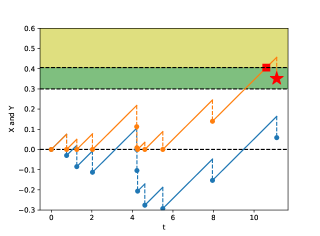
$n\mapsto L_{n},R_{n}$ when $\theta>0$	$t\mapsto X_{t},Y_{t}$ when $\theta>0$
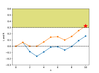
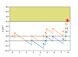
$n\mapsto L_{n},R_{n}$ when $\theta<0$	$t\mapsto X_{t}^{(|\kappa(\theta)|)}-|\kappa(\theta)|,Y_{t}^{(|\kappa(\theta)|)}-|\kappa(\theta)|$ when $\theta<0$

Figure 1. Sample paths of LLR (blue) and CUSUM (orange) and the corresponding generalized Sparre-Andersen process (blue) and its reflected process (orange) for $\theta>0$ and $\theta<0$ when $A=0.3$. (Top) The LLR process $L$ and the CUSUM statistic $R$ on the left plot and the corresponding generalized Sparre-Andersen process $X$ and its reflected process $Y$ on the right plot for the case $\theta>0$. The star indicates the time when $R$ exceeds $A$ for the first time. In the right plot, the square shows the first time $Y$ goes above $A+\kappa(\theta)=0.40536$ and the star shows the first jump time afterwards. Note that $R_{n}=Y_{\eta_{n}}$ for all $n\geq 0$. (Bottom) Similar plots for the case $\theta<0$, except that the right figure shows $X^{(|\kappa(\theta)|)}-|\kappa(\theta)|,Y^{(|\kappa(\theta)|)}-|\kappa(\theta)|$, which are translations of $X^{(|\kappa(\theta)|)}$ and $Y^{(|\kappa(\theta)|)}$. The time $\tau^{(|\kappa(\theta)|)}_{A+|\kappa(\theta)|}$ indicated by the star is the same as the time $Y^{(|\kappa(\theta)|)}-|\kappa(\theta)|$ crosses $A$. Note that $R_{n}=Y_{\eta_{n}}^{(|\kappa(\theta)|)}-|\kappa(\theta)|$ for $n\geq 0$.

Proposition 2.

Fix $A>0$ and let $\zeta$ be any strictly positive sequence. The following holds a.s.

1. When $\theta>0$, $R_{n}=Y_{\eta_{n}}$ for $n\geq 0$ and $T_{A}=1+N_{\tau_{A+\kappa(\theta)}}$.

2. When $\theta<0$, $R_{n}=Y_{\eta_{n}}^{(|\kappa(\theta)|)}-|\kappa(\theta)|$ for $n\geq 0$ and $T_{A}=N_{\tau^{(|\kappa(\theta)|)}_{A+|\kappa(\theta)|}}$.

Proof.

(1) Suppose $\theta>0$ (and then $\kappa(\theta)>0$). In view of Remark 1(1), the running infimum process $\underline{X}$ is updated only immediately after (negative) jumps and hence $\min_{1\leq k\leq n}X_{\eta_{k}}\wedge 0=\underline{X}_{\eta_{n}}$ implying, together with (13), $\underline{L}_{n}=\underline{X}_{\eta_{n}}$ for all $n\geq 0$. Therefore (4) becomes

$$R_{n}=X_{\eta_{n}}-\underline{X}_{\eta_{n}}=Y_{\eta_{n}},\quad n\geq 0.$$

If $R_{n}=Y_{\eta_{n}}>0$ then no reflection is made at $\eta_{n}$ (jump size is exactly $-\kappa(\theta)$) and necessarily $R_{n}=Y_{\eta_{n}}=Y_{\eta_{n}-}-\kappa(\theta)>0$. Therefore, for $A>0$, using that $X$ has only negative jumps,

$$T_{A} =\inf\{n\geq 1:Y_{\eta_{n}-}-\kappa(\theta)>A\}$$

$$=1+\#\textrm{\{jumps of $X$ (or $N$) before the instance $Y$ exceeds $A+\kappa(\theta)$\}}$$

$$=1+N_{\tau_{A+\kappa(\theta)}}$$

where the addition of $1$ is needed because we also need to count the last observation, which is the jump occurring after $Y$ crosses $A+\kappa(\theta)$ upward (and then lands on somewhere above $A$); see Figure 1.

(2) Suppose $\theta<0$ (and then $\kappa(\theta)<0$). Because $X_{\eta_{n}}=X_{\eta_{n}-}-\kappa(\theta)=X_{\eta_{n}-}+|\kappa(\theta)|=X_{\eta_{n}-}^{|\kappa(\theta)|}$, by (13),

$$\underline{L}_{n}=\min_{1\leq k\leq n}X_{\eta_{k}}\wedge 0=\min_{1\leq k\leq n}(X_{\eta_{k}-}^{(|\kappa(\theta)|)})\wedge 0.$$

In view of Remark 1(2), $X$ has a negative drift with positive jumps and hence $\min_{1\leq k\leq n}X_{\eta_{k}-}^{(|\kappa(\theta)|)}=\underline{X}_{\eta_{n}}^{(|\kappa(\theta)|)}$ and therefore $\underline{L}_{n}=\underline{X}_{\eta_{n}}^{(|\kappa(\theta)|)}\wedge 0$. Substituting this in (4),

$$R_{n}=X_{\eta_{n}}-\underline{X}_{\eta_{n}}^{(|\kappa(\theta)|)}\wedge 0=X_{\eta_{n}}^{(|\kappa(\theta)|)}-|\kappa(\theta)|-\underline{X}_{\eta_{n}}^{(|\kappa(\theta)|)}\wedge 0=Y_{\eta_{n}}^{(|\kappa(\theta)|)}-|\kappa(\theta)|,\quad n\geq 0.$$

Therefore (again see Figure 1),

$$T_{A} =\inf\{n\geq 1:Y_{\eta_{n}}^{(|\kappa(\theta)|)}-|\kappa(\theta)|>A\}$$

$$=\#\textrm{\{jumps of $X$ (or $N$) before or at the instance $Y^{(|\kappa(\theta)|)}$ exceeds $A+|\kappa(\theta)|$\}}$$

$$=N_{\tau^{(|\kappa(\theta)|)}_{A+|\kappa(\theta)|}}.$$

∎

3. First passage analysis of Sparre-Andersen processes with phase-type interarrivals

In the last section, we discussed in Proposition 2 that the CUSUM statistic can be written in terms of the reflection of the process (10), whose interarrival times are given by the observation $\zeta$. In particular, this reduces to an ordinary Sparre-Andersen process if the observations $\zeta$ are i.i.d. In this section, we derive new identities in the fluctuation theory of Sparre-Andersen processes with PH interarrivals. Although our main motivation of this section is its application in the computation of the optimal barrier (5) in the minimax formulation (see Section 3.3), we consider a wider class of Sparre-Andersen processes, not necessarily with jumps of constant size, which have applications in research areas beyond the study of the CUSUM procedure. These results are further generalized to non-i.i.d. settings in Section 5.

We denote, by $\mathcal{PH}(E,\boldsymbol{\alpha},\boldsymbol{T},\boldsymbol{t})$, a PH distribution with representation $(E,{\boldsymbol{{\alpha}}},\boldsymbol{T},\boldsymbol{t})$. In other words, it is the distribution of the first absorption time of a finite-state continuous-time Markov chain on the state space $E\cup\{\Delta\}$, consisting of the set of $\mathfrak{n}(\geq 1)$ transient states $E:=(1,2,\ldots,\mathfrak{n})$ and a single absorbing state $\Delta$. Its initial distribution on $E$ is given by the $\mathfrak{n}$-dimensional row vector $\boldsymbol{\alpha}=(\boldsymbol{\alpha}_{1},\ldots,\boldsymbol{\alpha}_{\mathfrak{n}})$ (the probability of starting at $\Delta$ is zero) such that $\sum_{i=1}^{\mathfrak{n}}{\boldsymbol{{\alpha}}}_{i}=1$ and transition rate matrix is given by

$$\left(\begin{array}[]{ll}\boldsymbol{T}&\boldsymbol{t}\\ \boldsymbol{0}^{\top}&0\end{array}\right).$$

Here, the sub-intensity matrix $\boldsymbol{T}$ shows the transition rates among those in $E$ and the exit rate vector $\boldsymbol{t}$ shows the rate of absorbing to $\Delta$ from each state in $E$. We allow the Markov chain to be defective in the sense that

$$\boldsymbol{q}:=-\boldsymbol{T}\boldsymbol{1}-\boldsymbol{t}\geq\boldsymbol{0}$$ (14)

is not necessarily $\boldsymbol{0}$; in other words, it is killed and sent to a cemetery state with rate $\boldsymbol{q}_{i}$ while it is in phase $i\in E$. Here and throughout the paper, let $\boldsymbol{1}=(1,\ldots,1)^{\top}$ and $\boldsymbol{0}=(0,\ldots,0)^{\top}$ be the column vectors consisting of all ones and all zeros, respectively (with dimensions clear from the context).

On a probability space $(\Omega,\mathcal{E},\mathbb{P})$, define the Sparre-Andersen process

$$X_{t}:=X_{0}+\gamma t-S_{N_{t}},\qquad t\geq 0,$$ (15)

where

$$S_{n}:=\sum_{i=1}^{n}C_{i},\quad n\geq 0.\$$ (16)

Here, we assume the drift is strictly positive ($\gamma>0$), $N=(N_{t})_{t\geq 0}$ is a renewal process with independent $\mathcal{PH}(E,\boldsymbol{\alpha},\boldsymbol{T},\boldsymbol{t})$-distributed interarrival times (a.k.a. PH renewal process) and $C=(C_{i})_{i\geq 1}$ is an i.i.d. sequence of $(0,\infty)$-valued random variables independent of $N$.

Remark 3.

The process (10) for the analysis of the CUSUM statistic when $\theta>0$ and $\zeta$ are i.i.d. is a special case of (15) with $\gamma=\theta$, deterministic jumps of size $C\equiv\kappa(\theta)>0$, and the observation $\zeta_{n}\sim\mathcal{PH}(E,\boldsymbol{\alpha},\boldsymbol{T},\boldsymbol{t})$ for all $n\geq 1$. The case $\theta<0$ can be dealt by considering its dual process (see Section 3.2).

It is a common practice to write (15) as a (spectrally negative) MAP. As in [4, Example 1.1, Chap. XI], the renewal process $N$ can be described as the number of arrivals of a background Markov chain $J$ with transition rate matrix $\boldsymbol{T}+\boldsymbol{B}$ where $\boldsymbol{T}$ and $\boldsymbol{B}:={\boldsymbol{t}}{\boldsymbol{{\alpha}}}$ are the intensities of transitions without arrivals and with arrivals, respectively. At each arrival that occurs with rate ${\boldsymbol{t}}$, $N$ jumps up by one and $J$ is reset according to the distribution ${\boldsymbol{{\alpha}}}$. We refer the reader to [4, Ch. XI] for a review of Markov arrival processes. With the background process $J$ as a modulator, we describe (15) as the ordinator of the MAP $(X,J)$, which experiences negative jumps of size $C$ upon arrivals (jump times of $N$).

We let $\mathbb{P}_{x,i}(\cdot)$ (with parentheses) be the law of $(X,J)$ when $(X_{0},J_{0})=(x,i)$ for $x\in\mathbb{R}$ and $i\in E$. We also write $\mathbb{P}_{x}[A,J_{\tau}]$ (with brackets) for the $\mathfrak{n}\times\mathfrak{n}$ matrix whose $(i,j)$-th element is $\mathbb{P}_{x,i}(A,J_{\tau}=j)$, for any event $A$ and (random or deterministic) time $\tau$. In particular, $\mathbb{P}_{x}[J_{\tau}]_{ij}=\mathbb{P}_{x,i}(J_{\tau}=j)$, $i,j\in E$. Analogously, we let $\mathbb{E}_{x}[Y;J_{\tau}]$ be the matrix of expectations of $\mathbb{E}_{x,i}(Y;J_{\tau}=j)$. We drop the subscript when $X_{0}=0$. Different from (10), we omit the superscript $(x)$ for the starting value, which can be modeled by using the measure $\mathbb{P}_{x}$.

Remark 4.

Note that (15) is more general than (10), and to avoid confusion we use different fonts for the probability/expectation operators from those in Section 2.1.

A so-called matrix exponent of the MAP $(X,J)$ is then given by

$$\boldsymbol{F}(s):=\gamma s\boldsymbol{I}_{\mathfrak{n}}+\boldsymbol{T}+\mathbb{E}(e^{-sC_{1}})\boldsymbol{B},\quad s\geq 0,$$ (17)

and it satisfies

$$\mathbb{E}[e^{s(X_{t}-X_{0})};J_{t}]=e^{\boldsymbol{F}(s)t},\quad t\geq 0,$$

where $\boldsymbol{I}_{\mathfrak{n}}$ is the $\mathfrak{n}\times\mathfrak{n}$ identity matrix. By convention it is assumed that $X$ is killed when $J$ is killed (sent to a cemetery state), which occurs with rate vector $\boldsymbol{q}$ as in (14).

3.1. Fluctuation theory of Sparre-Andersen process

There is a rich fluctuation theory for spectrally negative MAPs [14, 15, 28, 32], and the basic object underlying various identities is a so-called scale matrix $\boldsymbol{W}:[0,\infty)\to\mathbb{R}^{\mathfrak{n}\times\mathfrak{n}}$. This continuous, right-differentiable, matrix-valued function is characterized by the transform:

$$\int_{0}^{\infty}e^{-sx}\boldsymbol{W}(x)\mathrm{d}x=\boldsymbol{F}(s)^{-1}$$

for $s>\max\{\Re(z):z\in\mathbb{C},\det(\boldsymbol{F}(z))=0\}$. See, e.g., [28, Thm. 1]. Moreover, $\boldsymbol{W}(x)$ is invertible for $x>0$. We also write its integral $\overline{\boldsymbol{W}}(x):=\int_{0}^{x}\boldsymbol{W}(z)\mathrm{d}z$ and right-hand derivative $\boldsymbol{W}^{\prime}_{+}(x)$ for $x\geq 0$.

Remark 5.

In the following, we use several results of  [28] where the Markov chain $J$ is assumed to be irreducible, which is not the case below in this paper. It can be checked that this assumption is indeed redundant, given that the quantity

$$\psi(s)=\max_{i}\{\Re(\lambda_{i}(s)):\lambda_{i}(s)\text{ is an eigenvalue of }\boldsymbol{F}(s)\}$$

is treated with some care. In general, it should not be called the Perron-Frobenius eigenvalue, and we should not rely on $\psi^{\prime}(0)$ or the asymptotic drift concept. In particular, all the results in [28] apart from Cor. 4 (in the given form) hold without irreducibility assumption.

We refer the reader to [28] for a list of expectations one can compute using the scale matrix. Here, we focus on the identities relevant to the performance measures of the CUSUM procedure.

As in (11) and (12), we define the reflected process

$$Y_{t}:=X_{t}-\underline{X}_{t}\wedge 0,\quad t\geq 0,$$

where $\underline{X}_{t}:=\inf_{0\leq s\leq t}X_{s}$, and its first passage time

$$\tau_{a}:=\inf\{t\geq 0:Y_{t}>a\},\qquad a>0.$$ (18)

For $a>0$, by [28, Thm. 2],

$$\mathbb{P}[J_{\tau_{a}}]=\Big{(}\boldsymbol{I}_{\mathfrak{n}}-\overline{\boldsymbol{W}}(a)\boldsymbol{F}(0)\Big{)}^{-1}=\Big{(}\boldsymbol{I}_{\mathfrak{n}}-\overline{\boldsymbol{W}}(a)(\boldsymbol{T}+\boldsymbol{B})\Big{)}^{-1}.$$ (19)

Let the number of arrivals coming from phase $k\in E$ counted until $\tau_{a}$ be denoted by

$$N_{\tau_{a}}(k):=\sum_{t\leq\tau_{a}:\Delta N_{t}\neq 0}1_{\{J_{t-}=k\}}.$$ (20)

The following results can be derived easily by writing its generating function in terms of the scale matrix via (19). Its proof is deferred to Appendix B.1.

Lemma 6.

Suppose $J$ is non-defective (i.e. $\boldsymbol{q}=\boldsymbol{0}$). For $a>0$, we have

$$\mathbb{E}_{0,i}(N_{\tau_{a}}(k))=\Big{[}\Big{(}\boldsymbol{I}_{\mathfrak{n}}-\overline{\boldsymbol{W}}(a)(\boldsymbol{T}+\boldsymbol{B})\Big{)}^{-1}\overline{\boldsymbol{W}}(a)\mathrm{diag}({\boldsymbol{t}})\Big{]}_{ik},\quad i,k\in E,$$

and hence the unconditional expected number of arrivals until $\tau_{a}$ is

$$\mathbb{E}\big{(}N_{\tau_{a}}|J_{0}\sim{\boldsymbol{{\alpha}}}\big{)}=\sum_{i,k\in E}{\boldsymbol{{\alpha}}}_{i}\mathbb{E}_{0,i}(N_{\tau_{a}}(k))={\boldsymbol{{\alpha}}}\Big{(}\boldsymbol{I}_{\mathfrak{n}}-\overline{\boldsymbol{W}}(a)(\boldsymbol{T}+\boldsymbol{B})\Big{)}^{-1}\overline{\boldsymbol{W}}(a){\boldsymbol{t}}.$$

3.2. Spectrally positive case

By flipping the process (15), we can also consider the case with a negative drift and positive jumps. Suppose temporarily that, with the same $S$ and $N$ as in (15),

$$\textrm{(SP)}\qquad X_{t}=X_{0}-\gamma t+S_{N_{t}},\quad t\geq 0.$$ (21)

Then its dual process $X_{t}^{d}:=-X_{t}$ started at $X_{0}^{d}=-X_{0}$ admits the form (15). Let $\boldsymbol{W}^{d}(x)$ be the scale matrix for the spectrally negative MAP $(X^{d},J)$. Below it is understood that $\tau_{a}$ and (20) are for the original spectrally positive MAP $(X,J)$ and $\mathbb{P}_{x,i}$ is its law when $X_{0}=x$ (starting point of the original spectrally positive MAP) and $J_{0}=i$. Different from the spectrally negative case above, here we compute the first passage identities for a general starting point because for the analysis of CUSUM, we need the case the starting point is different from the reflection barrier $0$ (see Proposition 2(2)).

According to [28, Thm. 6], because $\boldsymbol{T}$ and $\boldsymbol{B}$ remain the same for $X^{d}$ and $X$,

$$\mathbb{P}_{x}[J_{\tau_{a}}]=\boldsymbol{I}_{\mathfrak{n}}-\Big{(}\overline{\boldsymbol{W}}^{d}(a-x)-\boldsymbol{W}^{d}(a-x)(\boldsymbol{W}^{d})^{\prime}_{+}(a)^{-1}{\boldsymbol{W}}^{d}(a)\Big{)}\big{(}\boldsymbol{T}+\boldsymbol{B}\big{)},\quad a>0,\;0\leq x\leq a.$$ (22)

The following is a direct consequence of this identity and hence we defer its proof to Appendix B.2.

Lemma 7.

Suppose (SP) as in (21) and $J$ is non-defective (i.e. $\boldsymbol{q}=\boldsymbol{0}$). For $a>0$ and $0\leq x\leq a$,

$$\mathbb{E}_{x,i}(N_{\tau_{a}}(k))=-\Big{[}\Big{(}\overline{\boldsymbol{W}}^{d}(a-x)-\boldsymbol{W}^{d}(a-x)(\boldsymbol{W}^{d})^{\prime}_{+}(a)^{-1}{\boldsymbol{W}}^{d}(a)\Big{)}\mathrm{diag}({\boldsymbol{t}})\Big{]}_{ik},\quad i,k\in E,$$

and hence the unconditional expected number of arrivals until $\tau_{a}$ is

$$\mathbb{E}_{x}(N_{\tau_{a}}|J_{0}\sim{\boldsymbol{{\alpha}}})=-{\boldsymbol{{\alpha}}}\Big{(}\overline{\boldsymbol{W}}^{d}(a-x)-\boldsymbol{W}^{d}(a-x)(\boldsymbol{W}^{d})^{\prime}_{+}(a)^{-1}{\boldsymbol{W}}^{d}(a)\Big{)}{\boldsymbol{t}}.$$

3.3. The case of CUSUM

Now recall our discussions in Section 2.1. The optimal barrier in the minimax formulation is given by $A_{\beta}$ such that (5) holds, and for this computation we need the average run length $\mathrm{ARL}(T_{A})\equiv\mathrm{E}_{\infty}[T_{A}]$ for $A>0$. Here, we consider the case $\zeta_{n}\sim F_{0}\sim\mathcal{PH}(E,\boldsymbol{\alpha},\boldsymbol{T},\boldsymbol{t})$ for all $n\geq 1$, and this defines the Markov chain $J$. Recall again that any positive distribution can be approximated by PH distributions.

1. Suppose $\theta>0$. Let ${\boldsymbol{W}}$ be the scale matrix of the MAP $(X,J)$ as in (15) with $\gamma=\theta>0$ and $C\equiv\kappa(\theta)>0$ (see Remark 3). In view of Proposition 2(1), Lemma 6 gives

   $$\begin{split}\mathrm{ARL}(T_{A})&=1+\mathbb{E}(N_{\tau_{A+\kappa(\theta)}}|J_{0}\sim{\boldsymbol{{\alpha}}})\\ &=1+{\boldsymbol{{\alpha}}}\Big{(}\boldsymbol{I}_{\mathfrak{n}}-\overline{\boldsymbol{W}}(A+\kappa(\theta))(\boldsymbol{T}+\boldsymbol{B})\Big{)}^{-1}\overline{\boldsymbol{W}}(A+\kappa(\theta)){\boldsymbol{t}},\quad A>0.\end{split}$$ (23)

2. Suppose $\theta<0$. Let ${\boldsymbol{W}}^{d}$ be the scale matrix of the MAP $(X^{d},J)$ as in (15) with $\gamma=-\theta>0$ and $C\equiv|\kappa(\theta)|=-\kappa(\theta)>0$ (again see Remark 3). In view of Proposition 2(2), Lemma 7 gives

   $$\begin{split}\mathrm{ARL}(T_{A})&=\mathbb{E}_{|\kappa(\theta)|}(N_{\tau_{A+|\kappa(\theta)|}}|J_{0}\sim{\boldsymbol{{\alpha}}})\\ &=-{\boldsymbol{{\alpha}}}\Big{(}\overline{\boldsymbol{W}}^{d}(A)-\boldsymbol{W}^{d}(A)(\boldsymbol{W}^{d})^{\prime}_{+}(A+|\kappa(\theta)|)^{-1}{\boldsymbol{W}}^{d}(A+|\kappa(\theta)|)\Big{)}{\boldsymbol{t}},\quad A>0.\end{split}$$ (24)

4. Series expansion of the scale matrix

As discussed in the previous section, the computation of the identities of interest boils down to that of the scale matrix. Here, we derive a new formula for $\boldsymbol{W}$ of the spectrally negative MAP $(X,J)$ of the form (15), generalizing the series expansion in [33, Thm. 2.2] for the Cramér-Lundberg model (i.e. $N$ is a Poisson process) and also [1, Thm. 2] in the case of Erlang interarrival times and deterministic jumps. These previous results were obtained by transform inversion, which becomes infeasible in this more general setting. Hence, we take a different approach.

For every $k\geq 1$ we define an $\mathfrak{n}k\times\mathfrak{n}k$ sub-transition rate matrix $\boldsymbol{T}_{k}$ and $\mathfrak{n}k\times\mathfrak{n}$ matrices $\boldsymbol{e}_{k1}$ and $\boldsymbol{e}_{kk}$:

$$\boldsymbol{T}_{k}=\begin{pmatrix}\boldsymbol{T}&\boldsymbol{B}&\ldots&\boldsymbol{O}\\ &\ddots&\ddots&\vdots\\ \vdots&&\boldsymbol{T}&\boldsymbol{B}\\ \boldsymbol{O}&\ldots&&\boldsymbol{T}\end{pmatrix},\qquad\boldsymbol{e}_{k1}=\begin{pmatrix}\boldsymbol{I}_{\mathfrak{n}}\\ \boldsymbol{O}\\ \vdots\\ \boldsymbol{O}\end{pmatrix},\qquad\boldsymbol{e}_{kk}=\begin{pmatrix}\boldsymbol{O}\\ \vdots\\ \boldsymbol{O}\\ \boldsymbol{I}_{\mathfrak{n}}\end{pmatrix},$$ (25)

so that $\boldsymbol{T}_{1}=\boldsymbol{T}$ and $\boldsymbol{e}_{11}=\boldsymbol{I}_{\mathfrak{n}}$. Here and for the rest of the paper, $\boldsymbol{O}$ is a zero matrix of appropriate dimension. These definitions are motivated by the identity

$$\mathbb{P}[N_{t}=k-1,J_{t}]=\boldsymbol{e}^{\top}_{k1}e^{\boldsymbol{T}_{k}t}\boldsymbol{e}_{kk},\qquad t\geq 0,\;k\geq 1,$$ (26)

which gives the matrix of probabilities of seeing $k-1$ arrivals by time $t$ and being in a particular phase at this time.

Theorem 8.

The scale matrix of a MAP in (15) has the representation

$$\boldsymbol{W}(x)=\frac{1}{\gamma}\sum_{k\geq 1}\int_{y\in[0,x]}\boldsymbol{e}^{\top}_{k1}e^{\boldsymbol{T}_{k}(y-x)/\gamma}\boldsymbol{e}_{kk}\mathbb{P}(S_{k-1}\in\mathrm{d}y),\qquad x\geq 0,$$

where $S$ is defined as in (16) with the understanding that $S_{0}=0$.

It is important to point out that the above series is absolutely convergent for any $x\geq 0$. Indeed, consider the matrix norm $\|\boldsymbol{M}\|:=\max_{i}\sum_{j}|\boldsymbol{M}_{ij}|$, and note that $\|\boldsymbol{T}_{k}\|\leq\|\boldsymbol{T}\|+\|\boldsymbol{B}\|=:r$, which is independent of $k$. Thus $\|\boldsymbol{e}^{\top}_{k1}e^{\boldsymbol{T}_{k}(y-x)/\gamma}\boldsymbol{e}_{kk}\|\leq e^{r|y-x|/\gamma}$ and also

$$\|\boldsymbol{W}(x)\|\leq\frac{1}{\gamma}\sum_{k\geq 1}\int_{y\in[0,x]}e^{r|y-x|/\gamma}\mathbb{P}(S_{k-1}\in\mathrm{d}y)\leq\frac{1}{\gamma}e^{rx/\gamma}\sum_{k\geq 1}\mathbb{P}(S_{k-1}\leq x)<\infty,$$ (27)

where finiteness of the latter sum follows from the basic renewal theory.

Remark 9.

The term $\boldsymbol{e}^{\top}_{k1}e^{\boldsymbol{T}_{k}(y-x)/\gamma}\boldsymbol{e}_{kk}$, $k\geq 1$, is the top-right corner block of $e^{\boldsymbol{T}_{k}(y-x)/\gamma}$, and can be written in an alternative way to avoid high dimensionality when computing it; see Appendix A.

Proof of Theorem 8.

First, we assume that $(X,J)$ is a killed process with $\boldsymbol{q}_{i}=q>0$ for all $i\in E$. As in  [28, Thm. 1 and (10)] (see also [28, Eq. (12)]), we can write

$$\boldsymbol{W}(x)=e^{-\boldsymbol{G}x}\boldsymbol{H}(0)-\boldsymbol{H}(-x),\qquad x>0,$$ (28)

where $\boldsymbol{G}$ is the transition rate matrix of the first passage Markov chain (i.e. $\mathbb{P}[J(\sigma_{x})]=\exp(\boldsymbol{G}x)$ for $x>0$ where $\sigma_{x}:=\inf\{t>0:X_{t}>x\}$) and $\boldsymbol{H}(x)$ denotes the matrix of expected occupation times at the level $x$; see [28, Sec. 4] for the precise definitions. In the present setting (where $X$ is of bounded variation and $0$ is irregular for itself), $\gamma\boldsymbol{H}(x)_{ij}$ is the expected number of times the level $x$ is hit in phase $j$ when starting in phase $i$. Moreover, there is a standard identity

$$\boldsymbol{H}(x)=e^{\boldsymbol{G}x}\boldsymbol{H}(0),\qquad x\geq 0,$$ (29)

which follows by the strong Markov property and additivity of occupation times together with the lack of positive jumps of $X$.

Consider the $\mathfrak{n}\times\mathfrak{n}$ matrix of probabilities of hitting the level $x\in\mathbb{R}$ in stage $k\geq 1$ (between $k-1$ and $k$th arrivals):

$$\int_{y\geq 0,y+x\geq 0}\boldsymbol{e}^{\top}_{k1}e^{\boldsymbol{T}_{k}(y+x)/\gamma}\boldsymbol{e}_{kk}\mathbb{P}(S_{k-1}\in\mathrm{d}y),$$

where the $i$-th row corresponds to starting in phase $i$ and the $j$-th column to hitting in phase $j$. This identity readily follows by conditioning on $S_{k-1}\geq 0$ which is independent of the rest, and then applying (26). By summing up this expression over $k$, we get

$$\boldsymbol{H}(x)=\frac{1}{\gamma}\sum_{k\geq 1}\int_{y\geq(-x)\vee 0}\boldsymbol{e}^{\top}_{k1}e^{\boldsymbol{T}_{k}(y+x)/\gamma}\boldsymbol{e}_{kk}\mathbb{P}(S_{k-1}\in\mathrm{d}y),\qquad x\in\mathbb{R}.$$

Next, we consider the cases $x\geq 0$ and $x<0$ separately and employ (29) to find

$$e^{\boldsymbol{G}x}\boldsymbol{H}(0) =\frac{1}{\gamma}\sum_{k\geq 1}\int_{y\geq 0}\boldsymbol{e}^{\top}_{k1}e^{\boldsymbol{T}_{k}(y+x)/\gamma}\boldsymbol{e}_{kk}\mathbb{P}(S_{k-1}\in\mathrm{d}y),\qquad x\geq 0,$$ (30)

$$\boldsymbol{H}(-x) =\frac{1}{\gamma}\sum_{k\geq 1}\int_{y>x}\boldsymbol{e}^{\top}_{k1}e^{\boldsymbol{T}_{k}(y-x)/\gamma}\boldsymbol{e}_{kk}\mathbb{P}(S_{k-1}\in\mathrm{d}y),\qquad x>0.$$

In the latter we use the fact that $y=x$ results in a zero matrix unless $k=1$, which can be disregarded because $S_{0}=0<x$.

We now show that the equality (30) holds also for $x<0$ by analytic continuation. First, $e^{\boldsymbol{G}x}\boldsymbol{H}(0)$ is a matrix of entire functions. To see that the right-hand side of (30) is also a matrix of entire functions, we first write it as

$$\frac{1}{\gamma}\sum_{k\geq 1}\boldsymbol{e}^{\top}_{k1}\mathbb{E}\big{(}e^{\boldsymbol{T}_{k}S_{k-1}/\gamma}\big{)}e^{\boldsymbol{T}_{k}x/\gamma}\boldsymbol{e}_{kk}.$$

As in (27) we see that the maximal absolute entry of $\frac{\boldsymbol{T}_{k}}{\gamma}e^{\boldsymbol{T}_{k}x/\gamma}$ is upper bounded by $\frac{r}{\gamma}e^{r|x|/\gamma}$ for all $x\in\mathbb{C},k\geq 1$. By noting that $\mathbb{E}(e^{\boldsymbol{T}_{k}S_{k-1}/\gamma})$ has $[0,1]$ entries we get a bound

$$\sum_{k\geq 1}\left\|\boldsymbol{e}^{\top}_{k1}\mathbb{E}\big{(}e^{\boldsymbol{T}_{k}S_{k-1}/\gamma}\big{)}\frac{\boldsymbol{T}_{k}}{\gamma}e^{\boldsymbol{T}_{k}x/\gamma}\boldsymbol{e}_{kk}\right\|\leq\frac{r}{\gamma}e^{r|x|/\gamma}\sum_{k\geq 1}\left\|\boldsymbol{e}^{\top}_{k1}\mathbb{E}\big{(}e^{\boldsymbol{T}_{k}S_{k-1}/\gamma}\big{)}\boldsymbol{e}_{kk}\right\|\leq re^{r|x|/\gamma}\sum_{i,j}\boldsymbol{H}(0)_{ij},$$

where in the latter step we upper bounded the matrix norm by the sum over all non-negative entries. In the defective case the matrix $\boldsymbol{H}(0)$ has finite entries [28, Lem. 10]. Now, according to, e.g., [51, A16] differentiation at any $x\in\mathbb{C}$ can be performed under the summation sign, as desired.

We can now apply analytic continuation to find that (30) holds when $x\geq 0$ is replaced by $-x$. Hence, (28) yields the stated expression of $\boldsymbol{W}(x)$ for $x>0$, whereas $\boldsymbol{W}(0)=\boldsymbol{I}_{\mathfrak{n}}/\gamma$ (see the comments following [28, Eq. (14)]) and so the formula is also true for $x=0$.

Finally, the non-defective case is obtained by a limit argument, by taking $q\downarrow 0$. It is known as in the proof of [28, Thm. 1] that $\boldsymbol{W}(x)$ is continuous in $q$, and so it is left to take the limit inside the sum and integral of the stated expression. Finally, by using the bound in (27) to see that the dominated convergence theorem applies, the proof is complete. ∎

For the case of deterministic jumps $C\equiv c>0$ as in the CUSUM case in Remark 3, the scale matrix can be written explicitly as a sum of matrix exponentials. In the next corollary, we also obtain the integrated/differentiated scale matrices, which are required in Lemmas 6 and 7. See Appendix A for alternative expressions.

Corollary 10.

Suppose $C\equiv c>0$. We have

$$\boldsymbol{W}(x) =\frac{1}{\gamma}\sum_{k=1}^{\lfloor x/c\rfloor+1}\boldsymbol{e}^{\top}_{k1}e^{\boldsymbol{T}_{k}(c(k-1)-x)/\gamma}\boldsymbol{e}_{kk}\qquad x\geq 0,$$ (31)

$$\boldsymbol{W}^{\prime}_{+}(x) =-\frac{1}{\gamma^{2}}\sum_{k=1}^{\lfloor x/c\rfloor+1}\boldsymbol{e}^{\top}_{k1}\boldsymbol{T}_{k}e^{\boldsymbol{T}_{k}(c(k-1)-x)/\gamma}\boldsymbol{e}_{kk},\qquad x>0,$$ (32)

$$\overline{\boldsymbol{W}}(x) =\sum_{k=1}^{\lfloor x/c\rfloor+1}\boldsymbol{e}^{\top}_{k1}\boldsymbol{T}_{k}^{-1}\Big{(}\boldsymbol{I}_{nk}-e^{\boldsymbol{T}_{k}(c(k-1)-x)/\gamma}\Big{)}\boldsymbol{e}_{kk},\qquad x\geq 0.$$ (33)

Proof.

The identity (31) is a direct consequence of Theorem 8 by using $S_{k-1}=c(k-1)$ for $k\geq 1$. The identities (32) and (33) can be derived by straightforward differentiation and integration of (31), where we also use Fubini’s theorem for the latter. ∎

We conclude this section with other important examples.

Example 11.

1. Suppose the distribution of the interarrival times of $N$ is defective exponential of rate $\lambda>0$ killed at rate $q\geq 0$. In other words it is exponential of rate $\lambda+q$ which is declared killed with probability $q/(\lambda+q)$. Thus $\boldsymbol{T}=-\lambda-q,{\boldsymbol{t}}=\lambda,{\boldsymbol{{\alpha}}}=1$ and we find that

   $$\boldsymbol{e}^{\top}_{k1}e^{\boldsymbol{T}_{k}x}\boldsymbol{e}_{kk}=\Big{(}\frac{\lambda}{\lambda+q}\Big{)}^{k-1}\frac{f_{k}(x;\lambda+q)}{\lambda+q},\qquad x>0,k\geq 1,$$

   where the function $f_{k}(x;\xi):=\xi^{k}x^{k-1}e^{-\xi x}/(k-1)!$ is the Erlang density. Theorem 8 now yields

   $$\boldsymbol{W}(x)=\frac{1}{\gamma}\sum_{k\geq 0}\frac{1}{k!}\Big{(}\frac{\lambda}{\lambda+q}\Big{)}^{k}\int_{y\in[0,x]}\big{(}(y-x)(\lambda+q)/\gamma\big{)}^{k}e^{-(y-x)(\lambda+q)/\gamma}\mathbb{P}(S_{k}\in\mathrm{d}y)\qquad x\geq 0,$$

   which coincides with the expression of the $q$-scale function of the Lévy process (for the process killed at rate $q$) considered in [33, Thm. 2.2].

2. In Corollary 10, suppose additionally that the interarrival times of $N$ have non-defective Erlang distribution on $\mathfrak{n}$ phases with rate $\lambda$. Then the $(i,j)$-th entry of $\boldsymbol{e}^{\top}_{k1}e^{\boldsymbol{T}_{k}x}\boldsymbol{e}_{kk}$ is given by $f_{k\mathfrak{n}-(i-1)-(\mathfrak{n}-j)}(x;\lambda)/\lambda$, which is understood as $0$ for $k=1,i>j$. Substituting this in (31) gives the formula in [1, Thm. 2].

5. Extension to the non-i.i.d. case with a change point

We now generalize the results of Section 3 to the non-i.i.d. case with a change point. To this end, we introduce another (this time, non-defective discrete-time) Markov chain, which changes states immediately after each arrival. The change point $\nu$ is given by its first entry time to a certain closed set and is hence discrete-time PH distributed. Furthermore, the distribution of the interarrival times is non-stationary and is modulated by this discrete-time Markov chain. This generalization lets us analyze the CUSUM procedure when the change point $\nu$ is discrete-time PH and observations $\zeta$ (corresponding to the interarrival times) are non-i.i.d. As we did in Section 3, we first obtain first passage identities for the general case and then specialize them for the analysis of CUSUM in Section 5.2.

More specifically, we let $Z=(Z_{0},Z_{1},\ldots)$ be a Markov chain on a state space $E^{\nu}_{0}\cup E^{\nu}_{1}$ with $|E^{\nu}_{0}|=m_{0}$ and $|E^{\nu}_{1}|=m_{1}$ and label each state by $E^{\nu}_{0}=\{(0,1),\ldots,(0,m_{0})\}$ and $E^{\nu}_{1}=\{(1,1),\ldots,(1,m_{1})\}$. The sets $E^{\nu}_{0}$ and $E^{\nu}_{1}$ correspond, respectively, to the pre- and post-change states so that the change point is expressed as

$$\nu=\inf(n\geq 0:Z_{n}\notin E^{\nu}_{0})=\inf(n\geq 0:Z_{n}\in E^{\nu}_{1}).$$ (34)

Necessarily $E^{\nu}_{1}$ is closed. We do not require $\nu<\infty$, but for the case this is certain $E^{\nu}_{0}$ is transient. We also allow $\nu=0$, or equivalently $Z_{0}\in E_{1}^{\nu}$, with a positive probability. In particular, if $m_{0}=1$ (resp. $m_{1}=1$) then the observations are i.i.d.  at or before (resp. after) $\nu$, conditionally given $\nu$.

Let the transition matrix and initial distribution of $Z$ be given by, respectively,

$$\begin{pmatrix}\boldsymbol{K}&\boldsymbol{L}\\ \boldsymbol{O}&\boldsymbol{M}\end{pmatrix}\quad\textrm{and}\quad\boldsymbol{\beta}=(\boldsymbol{\beta}_{1}^{(0)},\ldots,\boldsymbol{\beta}_{m_{0}}^{(0)},\boldsymbol{\beta}_{1}^{(1)},\ldots,\boldsymbol{\beta}^{(1)}_{m_{1}})$$ (35)

where $\boldsymbol{K}$ is $m_{0}\times m_{0}$, $\boldsymbol{L}$ is $m_{0}\times m_{1}$, and $\boldsymbol{M}$ is $m_{1}\times m_{1}$. When $\nu=0$ occurs with a positive probability, we have $\boldsymbol{\beta}_{l}^{(1)}>0$ for some $1\leq l\leq m_{1}$.

Example 12 (robustness).

One of our motivations for considering this non-i.i.d. model is to provide a method to analyze the robustness of the CUSUM procedure. One typical approach for evaluating robustness is to consider the case where, for a certain (usually small) probability $\epsilon>0$, the pre- and/or post-change distributions are different from the assumed $F_{0}$ and $F_{1}$ in the framework in Section 2.1.

As an illustration, suppose the post-change distribution is $F_{1}$ with probability $1-\epsilon$ and is $F_{2}$ with probability $\epsilon$. This can be modeled by setting $E_{1}^{\nu}=\{(1,1),(1,2)\}$ where on $(1,1)$ the observation is $F_{1}$-distributed whereas on $(1,2)$ it is $F_{2}$-distributed. Suppose further, for simplicity, that $\nu$ is zero-modified geometric

$$\mathbb{P}(\nu=k)=\left\{\begin{array}[]{ll}\mu,&k=0,\\ (1-\mu)(1-\lambda)^{k-1}\lambda,&k\geq 1,\end{array}\right.$$

for some $\mu\in[0,1)$ and $\lambda\in(0,1)$. We have $m_{0}=1$ and $m_{1}=2$ and the transition matrix and initial distribution of $Z$ as in (35) become, respectively,

$$\begin{pmatrix}1-\lambda&\lambda(1-\epsilon)&\lambda\epsilon\\ 0&1&0\\ 0&0&1\end{pmatrix}\quad\textrm{and}\quad(1-\mu,\mu(1-\epsilon),\mu\epsilon).$$

Above, the distribution of $\nu$ is assumed to be independent of whether the post-change distribution is $F_{1}$ or $F_{2}$, but the case it is dependent can be also modeled by a simple modification; see the example given in our numerical results in Section 6.2.

Example 13.

Besides the geometric distribution, classical examples of discrete-time PH distributions include negative binomial and mixed geometric distributions, which can be realized by writing $\boldsymbol{K}$ and $\boldsymbol{\beta}$ in an obvious way (see, e.g., [38]). In addition, $\mathrm{P}_{k}$ for $k\geq 1$ (where $\nu=k$ a.s.) in Section 2.1, which is of interest in the minimax formulation, can be modeled by using $k\times k$ matrix $\boldsymbol{K}$ with its entry $1$ on the first diagonal above the main diagonal and $0$ otherwise and $\boldsymbol{\beta}=(1,0,\ldots,0)$.

We replace the background Markov chain $J$ considered in Section 3 with a bivariate continuous-time Markov chain $(\tilde{J},\tilde{Z})=(\tilde{J}_{t},\tilde{Z}_{t})_{t\geq 0}$ defined as follows, and consider a new Markovian arrival process $\tilde{N}$. Here, $\tilde{Z}$ is a continuous-time Markov chain on $E^{\nu}_{0}\cup E^{\nu}_{1}$ embedded by $Z$ with the law (35) which changes states at each arrival so that

$$\tilde{Z}_{t}=Z_{\tilde{N}_{t}},\quad t\geq 0,$$ (36)

where the evolution of the arrival process $\tilde{N}$ is modeled as follows. Given $\tilde{Z}=(j,l)\in E^{\nu}_{0}\cup E^{\nu}_{1}$, the time until the next arrival is $\mathcal{PH}(E^{(j,l)},\boldsymbol{\alpha}^{(j,l)},\boldsymbol{T}^{(j,l)},\boldsymbol{t}^{(j,l)})$-distributed. This is modeled by $\tilde{J}$ whose initial distribution is $\boldsymbol{\alpha}^{(j,l)}$ and transition rate matrix $\boldsymbol{T}^{(j,l)}$. The arrival occurs at rate ${\boldsymbol{t}}^{(j,l)}$ and subsequently $\tilde{N}$ jumps up by one and $\tilde{Z}$ then changes its state according to its transition matrix given in (35).

In order to describe the law of the Markov chain $(\tilde{J},\tilde{Z})$, we label and order their states by

$$\tilde{E}^{\nu}_{0}\cup\tilde{E}^{\nu}_{1}:=\{(1,(0,1)),\ldots,(\mathfrak{n}^{(0,1)},(0,1)),\ldots,(1,(0,m_{0})),\ldots,(\mathfrak{n}^{(0,m_{0})},(0,m_{0})),\\ (1,(1,1)),\ldots,(\mathfrak{n}^{(1,1)},(1,1)),\ldots,(1,(1,m_{1})),\ldots,(\mathfrak{n}^{(1,m_{1})},(1,m_{1}))\},$$

where $\mathfrak{n}^{(i,l)}:=|E^{(i,l)}|$ for $(i,l)\in E^{\nu}_{0}\cup E^{\nu}_{1}$. The size of the state space $\tilde{E}^{\nu}_{0}\cup\tilde{E}^{\nu}_{1}$ is $\tilde{\mathfrak{n}}:=\sum_{l=1}^{m_{0}}\mathfrak{n}^{(0,l)}+\sum_{l=1}^{m_{1}}\mathfrak{n}^{(1,l)}$. The initial distribution is given by $\tilde{\mathfrak{n}}$-dimensional row vector

$$\tilde{{\boldsymbol{{\alpha}}}}:=(\boldsymbol{\beta}_{1}^{(0)}{\boldsymbol{{\alpha}}}^{(0,1)},\ldots,\boldsymbol{\beta}_{m_{0}}^{(0)}{\boldsymbol{{\alpha}}}^{(0,m_{0})},\boldsymbol{\beta}_{1}^{(1)}{\boldsymbol{{\alpha}}}^{(1,1)},\ldots,\boldsymbol{\beta}_{m_{1}}^{(1)}{\boldsymbol{{\alpha}}}^{(1,m_{1})}).$$

The transition intensity matrix is an $\tilde{\mathfrak{n}}\times\tilde{\mathfrak{n}}$ matrix $\tilde{\boldsymbol{T}}+\tilde{\boldsymbol{B}}$ where

$$\tilde{\boldsymbol{T}}:=\textrm{diag}(\boldsymbol{T}^{(0,1)},\ldots,\boldsymbol{T}^{(0,m_{0})},\boldsymbol{T}^{(1,1)},\ldots,\boldsymbol{T}^{(1,m_{1})})$$

is the non-arrival intensities whereas

$$\tilde{\boldsymbol{B}}:=\begin{pmatrix}\mathcal{K}&\mathcal{L}\\ \boldsymbol{O}&\mathcal{M}\end{pmatrix}$$

with

$$\mathcal{K} :=\begin{pmatrix}\boldsymbol{K}_{11}\boldsymbol{t}^{(0,1)}{\boldsymbol{{\alpha}}}^{(0,1)}&\ldots&\boldsymbol{K}_{1m_{0}}\boldsymbol{t}^{(0,1)}{\boldsymbol{{\alpha}}}^{(0,m_{0})}\\ \vdots&\ddots&\vdots\\ \boldsymbol{K}_{m_{0}1}\boldsymbol{t}^{(0,m_{0})}{\boldsymbol{{\alpha}}}^{(0,1)}&\ldots&\boldsymbol{K}_{m_{0}m_{0}}\boldsymbol{t}^{(0,m_{0})}{\boldsymbol{{\alpha}}}^{(0,m_{0})}\end{pmatrix},$$

$$\mathcal{L} :=\begin{pmatrix}\boldsymbol{L}_{11}\boldsymbol{t}^{(0,1)}{\boldsymbol{{\alpha}}}^{(1,1)}&\ldots&\boldsymbol{L}_{1m_{1}}\boldsymbol{t}^{(0,1)}{\boldsymbol{{\alpha}}}^{(1,m_{1})}\\ \vdots&\ddots&\vdots\\ \boldsymbol{L}_{m_{0}1}\boldsymbol{t}^{(0,m_{0})}{\boldsymbol{{\alpha}}}^{(1,1)}&\ldots&\boldsymbol{L}_{m_{0}m_{1}}\boldsymbol{t}^{(0,m_{0})}{\boldsymbol{{\alpha}}}^{(1,m_{1})}\end{pmatrix},$$

$$\mathcal{M} :=\begin{pmatrix}\boldsymbol{M}_{11}\boldsymbol{t}^{(1,1)}{\boldsymbol{{\alpha}}}^{(1,1)}&\ldots&\boldsymbol{M}_{1m_{1}}\boldsymbol{t}^{(1,1)}{\boldsymbol{{\alpha}}}^{(1,m_{1})}\\ \vdots&\ddots&\vdots\\ \boldsymbol{M}_{m_{1}1}\boldsymbol{t}^{(1,m_{1})}{\boldsymbol{{\alpha}}}^{(1,1)}&\ldots&\boldsymbol{M}_{m_{1}m_{1}}\boldsymbol{t}^{(1,m_{1})}{\boldsymbol{{\alpha}}}^{(1,m_{1})}\end{pmatrix},$$

is the arrival intensities.

Example 14.

In the setting of Example 12 where $F_{0}\sim\mathcal{PH}(E^{(0,1)},\boldsymbol{\alpha}^{(0,1)},\boldsymbol{T}^{(0,1)},\boldsymbol{t}^{(0,1)})$ and
$F_{l}\sim\mathcal{PH}(E^{(1,l)},\boldsymbol{\alpha}^{(1,l)},\boldsymbol{T}^{(1,l)},\boldsymbol{t}^{(1,l)})$ for $l=1,2$, we have

$$\tilde{{\boldsymbol{{\alpha}}}}=((1-\mu){\boldsymbol{{\alpha}}}^{(0,1)},\mu(1-\epsilon){\boldsymbol{{\alpha}}}^{(1,1)},\mu\epsilon{\boldsymbol{{\alpha}}}^{(1,2)})$$

and

$$\tilde{\boldsymbol{T}}=\begin{pmatrix}\boldsymbol{T}^{(0,1)}&\boldsymbol{O}&\boldsymbol{O}\\ \boldsymbol{O}&\boldsymbol{T}^{(1,1)}&\boldsymbol{O}\\ \boldsymbol{O}&\boldsymbol{O}&\boldsymbol{T}^{(1,2)}\end{pmatrix},\quad\tilde{\boldsymbol{B}}=\begin{pmatrix}(1-\lambda)\boldsymbol{t}^{(0,1)}\boldsymbol{\alpha}^{(0,1)}&\lambda(1-\epsilon)\boldsymbol{t}^{(0,1)}\boldsymbol{\alpha}^{(1,1)}&\lambda\epsilon\boldsymbol{t}^{(0,1)}\boldsymbol{\alpha}^{(1,2)}\\ \boldsymbol{O}&\boldsymbol{t}^{(1,1)}\boldsymbol{\alpha}^{(1,1)}&\boldsymbol{O}\\ \boldsymbol{O}&\boldsymbol{O}&\boldsymbol{t}^{(1,2)}\boldsymbol{\alpha}^{(1,2)}\end{pmatrix}.$$

We now consider the MAP $(X,(\tilde{J},\tilde{Z}))$ given by

$$X_{t}:=X_{0}+\gamma t-S_{\tilde{N}_{t}},\qquad t\geq 0,$$ (37)

with the same $S$ as in (16), as a generalization of (15). Because the only change made from (15) is the modulator of the MAP, whose law is completely specified by its transition rate matrix and its initial distribution, it is clear that Theorem 8 holds by simply replacing $\boldsymbol{T}$ and $\boldsymbol{B}$ with $\tilde{\boldsymbol{T}}$ and $\tilde{\boldsymbol{B}}$, respectively. Hence, we have the following.

Theorem 15.

The scale matrix of a MAP $(X,(\tilde{J},\tilde{Z}))$ as in (37) has the representation

$$\boldsymbol{W}(x)=\frac{1}{\gamma}\sum_{k\geq 1}\int_{y\in[0,x]}\tilde{\boldsymbol{e}}^{\top}_{k1}e^{\tilde{\boldsymbol{T}}_{k}(y-x)/\gamma}\tilde{\boldsymbol{e}}_{kk}\mathbb{P}(S_{k-1}\in\mathrm{d}y),\qquad x\geq 0,$$

where $\tilde{\boldsymbol{T}}_{k}$, $\tilde{\boldsymbol{e}}_{k1}$, and $\tilde{\boldsymbol{e}}_{kk}$ are as in (25) with $\boldsymbol{T}$, $\boldsymbol{B}$, and $\boldsymbol{I}_{\mathfrak{n}}$ replaced with $\tilde{\boldsymbol{T}}$, $\tilde{\boldsymbol{B}}$, and $\boldsymbol{I}_{\tilde{\mathfrak{n}}}$, respectively, for all $k\geq 1$.

Using this generalized scale matrix in Theorem 15, the identity (19) and Lemma 6 can be extended as follows. Below, it is understood that the first passage time $\tau_{a}$ as in (18) is for the generalized $X$ defined in (37). In view of (34) and (36),

$$\{\tilde{N}_{\tau_{a}}<\nu\}=\{Z_{1},\ldots,Z_{\tilde{N}_{\tau_{a}}}\in E_{0}^{\nu}\}=\{Z_{\tilde{N}_{\tau_{a}}}\in E_{0}^{\nu}\}=\{\tilde{Z}_{\tau_{a}}\in E_{0}^{\nu}\}$$ (38)

where in the second equality, we use that $E_{1}^{\nu}$ is closed. We let the $\tilde{\mathfrak{n}}$-dimensional column vectors

$$\tilde{{\boldsymbol{t}}}^{(0)} =[({\boldsymbol{t}}^{(0,1)})^{\top},\ldots,({\boldsymbol{t}}^{(0,m_{0})})^{\top},\boldsymbol{0}^{\top},\ldots,\boldsymbol{0}^{\top}]^{\top},$$

$$\tilde{{\boldsymbol{t}}}^{(1)} =[\boldsymbol{0}^{\top},\ldots,\boldsymbol{0}^{\top},({\boldsymbol{t}}^{(1,1)})^{\top},\ldots,({\boldsymbol{t}}^{(1,m_{1})})^{\top}]^{\top},$$

$$\tilde{{\boldsymbol{t}}} =\tilde{{\boldsymbol{t}}}^{(0)}+\tilde{{\boldsymbol{t}}}^{(1)}=[({\boldsymbol{t}}^{(0,1)})^{\top},\ldots,({\boldsymbol{t}}^{(0,m_{0})})^{\top},({\boldsymbol{t}}^{(1,1)})^{\top},\ldots,({\boldsymbol{t}}^{(1,m_{1})})^{\top}]^{\top},$$

be the rate of arrivals coming from $\tilde{E}_{0}^{\nu}$ and $\tilde{E}_{1}^{\nu}$ and their sum. We also let

$$\tilde{\boldsymbol{1}}^{(0)}=[\boldsymbol{1}^{\top},\ldots,\boldsymbol{1}^{\top},\boldsymbol{0}^{\top},\ldots,\boldsymbol{0}^{\top}]^{\top}\quad\textrm{and}\quad\tilde{\boldsymbol{1}}^{(1)}=[\boldsymbol{0}^{\top},\ldots,\boldsymbol{0}^{\top},\boldsymbol{1}^{\top},\ldots,\boldsymbol{1}^{\top}]^{\top},$$

whose element is $1$ or $0$ depending on whether it belongs to $\tilde{E}_{0}^{\nu}$ or $\tilde{E}_{1}^{\nu}$.

As for (20), we let $\tilde{N}_{\tau_{a}}(k):=\sum_{t\leq\tau_{a}:\Delta\tilde{N}_{t}\neq 0}1_{\{(\tilde{J}_{t-},\tilde{Z}_{t-})=k\}}$ for $a>0$ and $k\in\tilde{E}_{0}^{\nu}\cup\tilde{E}_{1}^{\nu}$.

Lemma 16.

(1) For $a>0$, we have

$$\mathbb{P}[(\tilde{J},\tilde{Z})_{\tau_{a}}]=\Big{(}\boldsymbol{I}_{\tilde{\mathfrak{n}}}-\overline{\boldsymbol{W}}(a)(\tilde{\boldsymbol{T}}+\tilde{\boldsymbol{B}})\Big{)}^{-1}.$$

Hence, by (38),

$$\mathbb{P}(\tilde{N}_{\tau_{a}}<\nu|(\tilde{J}_{0},\tilde{Z}_{0})\sim\tilde{{\boldsymbol{{\alpha}}}})=\mathbb{P}(\tilde{Z}_{\tau_{a}}\in E_{0}^{\nu}|(\tilde{J}_{0},\tilde{Z}_{0})\sim\tilde{{\boldsymbol{{\alpha}}}})=\tilde{{\boldsymbol{{\alpha}}}}\Big{(}\boldsymbol{I}_{\tilde{\mathfrak{n}}}-\overline{\boldsymbol{W}}(a)(\tilde{\boldsymbol{T}}+\tilde{\boldsymbol{B}})\Big{)}^{-1}\tilde{\boldsymbol{1}}^{(0)}.$$

(2) Suppose $(\tilde{J},\tilde{Z})$ is non-defective (i.e. $\boldsymbol{q}=\boldsymbol{0}$). For $a>0$, we have

$$\mathbb{E}_{0,i}(\tilde{N}_{\tau_{a}}(k))=\Big{[}\Big{(}\boldsymbol{I}_{\tilde{\mathfrak{n}}}-\overline{\boldsymbol{W}}(a)(\tilde{\boldsymbol{T}}+\tilde{\boldsymbol{B}})\Big{)}^{-1}\overline{\boldsymbol{W}}(a)\mathrm{diag}(\tilde{{\boldsymbol{t}}})\Big{]}_{ik},\quad i,k\in\tilde{E}_{0}^{\nu}\cup\tilde{E}_{1}^{\nu}.$$

Hence,

$$\mathbb{E}(\tilde{N}_{\tau_{a}}|(\tilde{J}_{0},\tilde{Z}_{0})\sim\tilde{{\boldsymbol{{\alpha}}}}) =\tilde{{\boldsymbol{{\alpha}}}}\Big{(}\boldsymbol{I}_{\tilde{\mathfrak{n}}}-\overline{\boldsymbol{W}}(a)(\tilde{\boldsymbol{T}}+\tilde{\boldsymbol{B}})\Big{)}^{-1}\overline{\boldsymbol{W}}(a)\tilde{{\boldsymbol{t}}},$$

$$\mathbb{E}\Big{(}\sum_{t\leq\tau_{a}:\Delta\tilde{N}_{t}\neq 0}1_{\{\tilde{Z}_{t-}\in E_{1}^{\nu}\}}\Big{|}(\tilde{J}_{0},\tilde{Z}_{0})\sim\tilde{{\boldsymbol{{\alpha}}}}\Big{)} =\tilde{{\boldsymbol{{\alpha}}}}\Big{(}\boldsymbol{I}_{\tilde{\mathfrak{n}}}-\overline{\boldsymbol{W}}(a)(\tilde{\boldsymbol{T}}+\tilde{\boldsymbol{B}})\Big{)}^{-1}\overline{\boldsymbol{W}}(a)\tilde{{\boldsymbol{t}}}^{(1)}.$$

5.1. Spectrally positive case

Suppose temporarily that

$$(\widetilde{\textrm{SP}})\qquad X_{t}=X_{0}-\gamma t+S_{\tilde{N}_{t}},\quad t\geq 0.$$ (39)

We use the same notations as those in Section 3.2, except that we replace $J$ by $(\tilde{J},\tilde{Z})$ and $N$ by $\tilde{N}$.

It is clear that (22) immediately gives, for this generalized case:

$$\mathbb{P}_{x}[(\tilde{J},\tilde{Z})_{\tau_{a}}]=\boldsymbol{I}_{\tilde{\mathfrak{n}}}-\Big{(}\overline{\boldsymbol{W}}^{d}(a-x)-\boldsymbol{W}^{d}(a-x)(\boldsymbol{W}^{d})^{\prime}_{+}(a)^{-1}{\boldsymbol{W}}^{d}(a)\Big{)}(\tilde{\boldsymbol{T}}+\tilde{\boldsymbol{B}}),\quad a>0,\;0\leq x\leq a.$$ (40)

Likewise, by Lemma 7, we have the following.

Lemma 17.

Suppose ($\widetilde{\textrm{SP}}$). For $a>0$ and $0\leq x\leq a$,

$$\mathbb{E}_{x,i}(\tilde{N}_{\tau_{a}}(k))=-\Big{[}\Big{(}\overline{\boldsymbol{W}}^{d}(a-x)-\boldsymbol{W}^{d}(a-x)(\boldsymbol{W}^{d})^{\prime}_{+}(a)^{-1}{\boldsymbol{W}}^{d}(a)\Big{)}\mathrm{diag}({\boldsymbol{t}})\Big{]}_{ik},\quad i,k\in E,$$

and hence

$$\mathbb{E}_{x}(\tilde{N}_{\tau_{a}}|(\tilde{J}_{0},\tilde{Z}_{0})\sim\tilde{{\boldsymbol{{\alpha}}}}) =-\tilde{{\boldsymbol{{\alpha}}}}\Big{(}\overline{\boldsymbol{W}}^{d}(a-x)-\boldsymbol{W}^{d}(a-x)(\boldsymbol{W}^{d})^{\prime}_{+}(a)^{-1}{\boldsymbol{W}}^{d}(a)\Big{)}\tilde{{\boldsymbol{t}}},$$

$$\mathbb{E}_{x}\Big{(}\sum_{t\leq\tau_{a}:\Delta\tilde{N}_{t}\neq 0}1_{\{\tilde{Z}_{t-}\in E_{1}^{\nu}\}}\Big{|}(\tilde{J}_{0},\tilde{Z}_{0})\sim\tilde{{\boldsymbol{{\alpha}}}}\Big{)} =-\tilde{{\boldsymbol{{\alpha}}}}\Big{(}\overline{\boldsymbol{W}}^{d}(a-x)-\boldsymbol{W}^{d}(a-x)(\boldsymbol{W}^{d})^{\prime}_{+}(a)^{-1}{\boldsymbol{W}}^{d}(a)\Big{)}\tilde{{\boldsymbol{t}}}^{(1)}.$$

5.2. The case of CUSUM

With the above results for the non-i.i.d. case, more interesting quantities can be computed beyond those obtained in Section 3.3. Here, we compute the average detection delay (8) and false alarm probability (9), in addition to the average run length (7).

Below, we consider the change point $\nu$ and observation $\zeta$, modeled by $(\tilde{J},\tilde{Z})$. As we did in Section 3.3, we shall first consider the case $\theta>0$ and then the case $\theta<0$.

5.2.1. For the case $\theta>0$

Let $\boldsymbol{W}$ be the scale matrix of the MAP $(X,(\tilde{J},\tilde{Z}))$ as in (37) with $\gamma=\theta$ and $C\equiv\kappa(\theta)>0$ (see Remark 3).

Corollary 18.

Fix $A>0$. (1) We have

$$\mathrm{PFA}(T_{A}) =\mathbb{P}\Big{(}\tilde{N}_{\tau_{A+\kappa(\theta)}}+1\leq\nu|(\tilde{J}_{0},\tilde{Z}_{0})\sim\tilde{{\boldsymbol{{\alpha}}}}\Big{)}=\tilde{{\boldsymbol{{\alpha}}}}\Big{(}\boldsymbol{I}_{\tilde{\mathfrak{n}}}-\overline{\boldsymbol{W}}(A+\kappa(\theta))(\tilde{\boldsymbol{T}}+\tilde{\boldsymbol{B}})\Big{)}^{-1}\tilde{\boldsymbol{1}}^{(0)}.$$

(2) We have

$$\mathrm{ARL}(T_{A}) =1+\mathbb{E}(\tilde{N}_{\tau_{A+\kappa(\theta)}}|(\tilde{J}_{0},\tilde{Z}_{0})\sim\tilde{{\boldsymbol{{\alpha}}}})$$

$$=1+\tilde{{\boldsymbol{{\alpha}}}}\Big{(}\boldsymbol{I}_{\tilde{\mathfrak{n}}}-\overline{\boldsymbol{W}}(A+\kappa(\theta))(\tilde{\boldsymbol{T}}+\tilde{\boldsymbol{B}})\Big{)}^{-1}\overline{\boldsymbol{W}}(A+\kappa(\theta))\tilde{{\boldsymbol{t}}},$$

$$\mathrm{ADD}(T_{A}) =\mathbb{E}\big{(}(\tilde{N}_{\tau_{A+\kappa(\theta)}}+1-\nu)^{+}|(\tilde{J}_{0},\tilde{Z}_{0})\sim\tilde{{\boldsymbol{{\alpha}}}}\big{)}$$

$$=\tilde{{\boldsymbol{{\alpha}}}}\Big{(}\boldsymbol{I}_{\tilde{\mathfrak{n}}}-\overline{\boldsymbol{W}}(A+\kappa(\theta))(\tilde{\boldsymbol{T}}+\tilde{\boldsymbol{B}})\Big{)}^{-1}\Big{(}\overline{\boldsymbol{W}}(A+\kappa(\theta))\tilde{{\boldsymbol{t}}}^{(1)}+\tilde{\boldsymbol{1}}^{(1)}\Big{)}.$$

Proof.

(1) By Proposition 2(1) and (38), $\{T_{A}\leq\nu\}=\{\tilde{N}_{\tau_{A+\kappa(\theta)}}+1\leq\nu\}=\{\tilde{N}_{\tau_{A+\kappa(\theta)}}<\nu\}=\{\tilde{Z}_{\tau_{A+\kappa(\theta)}}\in E_{0}^{\nu}\}$. Hence, Lemma 16(1) gives the results.

(2) The first claim is immediate by Proposition 2(1) and Lemma 16(2). For the second claim,

$$(T_{A}-\nu)^{+}=(\tilde{N}_{\tau_{A+\kappa(\theta)}}+1-\nu)^{+} =\Big{(}\sum_{t\leq\tau_{A+\kappa(\theta)}:\Delta\tilde{N}_{t}\neq 0}1_{\{\tilde{Z}_{t-}\in E_{1}^{\nu}\}}\Big{)}+1_{\{\tilde{Z}_{\tau_{A}+\kappa(\theta)}\in E_{1}^{\nu}\}}.$$

Hence, Lemma 16(1) and (2) give the result. ∎

Remark 19.

Notice that more variations can be computed. For example, in Examples 12 and 14, one can for example compute $\mathrm{P}(T_{A}>\nu,H_{l})$ and $\mathrm{E}((T_{A}-\nu)^{+};H_{l})$ where $H_{l}$ is the event that the true post-change distribution is $F_{l}$ for $l=1,2$. Indeed,

$$\{T_{A}>\nu,H_{l}\}=\{\tilde{N}_{\tau_{A+\kappa(\theta)}}+1>\nu,H_{l}\}=\{\tilde{N}_{\tau_{A+\kappa(\theta)}}\geq\nu,H_{l}\}=\{\tilde{Z}_{\tau_{A+\kappa(\theta)}}=(1,l)\},\quad l=1,2,$$

whose probability can be computed by Lemma 16(1). In addition, for $l=1,2$,

$$(T_{A}-\nu)^{+}1_{H_{l}}=(\tilde{N}_{\tau_{A+\kappa(\theta)}}+1-\nu)^{+}1_{H_{l}} =\Big{(}\sum_{t\leq\tau_{A+\kappa(\theta)}:\Delta\tilde{N}_{t}\neq 0}1_{\{\tilde{Z}_{t-}=(1,l)\}}\Big{)}+1_{\{\tilde{Z}_{\tau_{A}+\kappa(\theta)}=(1,l)\}},$$

whose expectation can be computed by Lemma 16(1) and (2).

5.2.2. For the case $\theta<0$

Let $\boldsymbol{W}^{d}$ be the scale matrix of the MAP $(X^{d},(\tilde{J},\tilde{Z}))$ as in (37) with $\gamma=-\theta>0$ and $C\equiv-\kappa(\theta)>0$ (see Remark 3).

We first obtain the average run length and average detection delay, which can be derived easily by Lemma 17.

Corollary 20.

Fix $A>0$. We have

$$\mathrm{ARL}(T_{A}) =\mathbb{E}_{|\kappa(\theta)|}\big{(}\tilde{N}_{\tau_{A+|\kappa(\theta)|}}|(\tilde{J}_{0},\tilde{Z}_{0})\sim\tilde{{\boldsymbol{{\alpha}}}}\big{)}$$

$$=-\tilde{{\boldsymbol{{\alpha}}}}\Big{(}\overline{\boldsymbol{W}}^{d}(A)-\boldsymbol{W}^{d}(A)(\boldsymbol{W}^{d})^{\prime}_{+}(A+|\kappa(\theta)|)^{-1}{\boldsymbol{W}}^{d}(A+|\kappa(\theta)|)\Big{)}\tilde{{\boldsymbol{t}}},$$

$$\mathrm{ADD}(T_{A}) =\mathbb{E}_{|\kappa(\theta)|}\big{(}(\tilde{N}_{\tau_{A+|\kappa(\theta)|}}-\nu)^{+}|(\tilde{J}_{0},\tilde{Z}_{0})\sim\tilde{{\boldsymbol{{\alpha}}}}\big{)}$$

$$=-\tilde{{\boldsymbol{{\alpha}}}}\Big{(}\overline{\boldsymbol{W}}^{d}(A)-\boldsymbol{W}^{d}(A)(\boldsymbol{W}^{d})^{\prime}_{+}(A+|\kappa(\theta)|)^{-1}{\boldsymbol{W}}^{d}(A+|\kappa(\theta)|)\Big{)}\tilde{{\boldsymbol{t}}}^{(1)}.$$

Proof.

The first claim is immediate by Proposition 2(2) and Lemma 17. Regarding the second claim, because given $X_{0}=|\kappa(\theta)|$, $(T_{A}-\nu)^{+}=(\tilde{N}_{\tau_{A+|\kappa(\theta)|}}-\nu)^{+}=\sum_{t\leq\tau_{A+|\kappa(\theta)|}:\Delta\tilde{N}_{t}\neq 0}1_{\{\tilde{Z}_{t-}\in E_{1}^{\nu}\}}$, Lemma 17 shows the result. ∎

On the other hand, the computation of the false alarm probability is more involved. By Proposition 2(2), given $X_{0}=|\kappa(\theta)|$, $\{T_{A}\leq\nu\}=\{\tilde{N}_{\tau_{A+|\kappa(\theta)|}}\leq\nu\}=\{\tilde{N}_{\tau_{A+|\kappa(\theta)|}}<\nu\}\cup\{\tilde{N}_{\tau_{A+|\kappa(\theta)|}}=\nu\}$. Here (38) holds for ($\widetilde{\textrm{SP}}$) as well and the probability of $\{\tilde{N}_{\tau_{A+|\kappa(\theta)|}}<\nu\}=\{\tilde{Z}_{\tau_{A+|\kappa(\theta)|}}\in E_{0}^{\nu}\}$ can be computed by (40). On the other hand, it is not clear if the probability of $\{\tilde{N}_{\tau_{A+|\kappa(\theta)|}}=\nu\}=\{\tilde{Z}_{\tau_{A+|\kappa(\theta)|}-}\in E_{0}^{\nu},\tilde{Z}_{\tau_{A+|\kappa(\theta)|}}\in E_{1}^{\nu}\}$ can be directly computed.

However, this can be dealt by considering a modification, say $\widehat{Z}$, of $Z$ by doubling the states $E^{\nu}_{1}$ to keep track of whether it first entered from $E^{\nu}_{0}$ or not. More precisely, we modify the state space of $Z$ to $E^{\nu}_{0}\cup E^{\nu}_{1^{\prime}}\cup E^{\nu}_{1}$ where $E^{\nu}_{1^{\prime}}$ is a copy of $E^{\nu}_{1}$. The Markov chain $\widehat{Z}$ moves from $E^{\nu}_{0}$ to $E^{\nu}_{1^{\prime}}$ and then to $E^{\nu}_{1}$. In particular, it stays only at a unit time in $E^{\nu}_{1^{\prime}}$. The change point is given by $\nu=\inf(n\geq 0:\widehat{Z}_{n}\notin E^{\nu}_{0})=\inf(n\geq 0:\widehat{Z}_{n}\in E^{\nu}_{1^{\prime}}\cup E^{\nu}_{1})$. As a modification of (35), the transition matrix and initial distribution of $\widehat{Z}$ are given by, respectively,

$$\begin{pmatrix}\boldsymbol{K}&\boldsymbol{L}&\boldsymbol{O}\\ \boldsymbol{O}&\boldsymbol{O}&\boldsymbol{M}\\ \boldsymbol{O}&\boldsymbol{O}&\boldsymbol{M}\end{pmatrix}\quad\textrm{and}\quad\boldsymbol{\beta}=(\boldsymbol{\beta}_{1}^{(0)},\ldots,\boldsymbol{\beta}_{m_{0}}^{(0)},\boldsymbol{\beta}_{1}^{(1)},\ldots,\boldsymbol{\beta}^{(1)}_{m_{1}},0,\ldots,0).$$ (41)

By replacing (35) with (41), $\tilde{E}^{\nu}_{0}\cup\tilde{E}^{\nu}_{1}$, $\tilde{{\boldsymbol{{\alpha}}}}$, $\tilde{\mathfrak{n}}$, $\tilde{\boldsymbol{T}}$ and $\tilde{\boldsymbol{B}}$ are modified accordingly to say, $\tilde{E}^{\nu}_{0}\cup\tilde{E}^{\nu}_{1^{\prime}}\cup\tilde{E}^{\nu}_{1}$, $\widehat{{\boldsymbol{{\alpha}}}}$, $\widehat{\mathfrak{n}}$, $\widehat{\boldsymbol{T}}$ and $\widehat{\boldsymbol{B}}$. However, these changes do not alter the law of $\tilde{J}$ nor the arrivals $\tilde{N}$. Following the same steps, we can compute (40) for this slightly generalized case. Indeed, given $X_{0}=|\kappa(\theta)|$,

$$\{T_{A}\leq\nu\}=\{\tilde{N}_{\tau_{A+|\kappa(\theta)|}}\leq\nu\}=\{\tilde{N}_{\tau_{A+|\kappa(\theta)|}}<\nu\}\cup\{\tilde{N}_{\tau_{A+|\kappa(\theta)|}}=\nu\}\\ =\{\widehat{Z}_{\tau_{A+|\kappa(\theta)|}}\in E_{0}^{\nu}\}\cup\{\widehat{Z}_{\tau_{A+|\kappa(\theta)|}}\in E_{1^{\prime}}^{\nu}\}=\{\widehat{Z}_{\tau_{A+|\kappa(\theta)|}}\in E_{0}^{\nu}\cup E_{1^{\prime}}^{\nu}\}.$$

By these and (40), the following is immediate.

Corollary 21.

Fix $A>0$. Let $\boldsymbol{W}^{d}$ be the scale function of the MAP $(X^{d},(\tilde{J},\widehat{Z}))$ as in (37) with $\gamma=-\theta>0$ and $C_{i}\equiv-\kappa(\theta)>0$ and $\widehat{Z}$ given by (41). We have

$$\mathrm{PFA}(T_{A}) =\mathbb{P}_{|\kappa(\theta)|}\Big{(}\tilde{N}_{\tau_{A+|\kappa(\theta)|}}\leq\nu|(\tilde{J}_{0},\widehat{Z}_{0})\sim\widehat{{\boldsymbol{{\alpha}}}}\Big{)}$$

$$=\widehat{{\boldsymbol{{\alpha}}}}\Big{[}\boldsymbol{I}_{\widehat{n}}-\Big{(}\overline{\boldsymbol{W}}^{d}(A)-\boldsymbol{W}^{d}(A)(\boldsymbol{W}^{d})^{\prime}_{+}(A+|\kappa(\theta)|)^{-1}{\boldsymbol{W}}^{d}(A+|\kappa(\theta)|)\Big{)}(\widehat{\boldsymbol{T}}+\widehat{\boldsymbol{B}})\Big{]}\widehat{\boldsymbol{1}},$$

where $\widehat{\boldsymbol{1}}:=[\boldsymbol{1}^{\top},\ldots,\boldsymbol{1}^{\top},\boldsymbol{1}^{\top},\ldots,\boldsymbol{1}^{\top},\boldsymbol{0}^{\top},\ldots,\boldsymbol{0}^{\top}]^{\top}$, whose element is $1$ if it belongs to $\tilde{E}_{0}^{\nu}\cup\tilde{E}_{1^{\prime}}^{\nu}$ and zero otherwise.

6. Numerical examples

We conclude the paper by confirming the analytical results obtained in the previous sections through numerical experiments. All codes are implemented in Python. Because the scale matrix grows exponentially fast, high precision is required for accurate results. Hence, we used the mpmath library with 30 digits. In addition, we compute the matrix exponentials in the scale function in an alternative way as described in Appendix A. We also used butools for randomly selecting the PH distributions used in our experiments.

We let $F_{0}$ be a PH distribution with initial distribution and transition rate matrix, respectively,

$$\boldsymbol{\alpha}=(0.28,0.35,0.37),\quad\boldsymbol{T}=\begin{pmatrix}-0.51&0.12&0.12\\ 0.21&-0.46&0.10\\ 0.28&0.16&-0.63\end{pmatrix}$$

and $F_{1}$ be the PH distribution obtained by the exponential tilting of $F_{0}$ for Case SN: $\theta=0.1$ and Case SP: $\theta=-0.1$. As in Remark 1, the corresponding continuous-time process $X$ defined in (10) becomes spectrally negative and spectrally positive, respectively. Below, we focus on the LLR process (1) with $f_{0}$ and $f_{1}$ being the densities of $F_{0}$ and $F_{1}$, respectively.

For the barrier $A$, we set it to be the optimal barrier $A_{\beta}$ in the minimax formulation that minimizes the Lorden detection measure (6) for $\beta=5$ and $\beta=10$, so that the average run length $\mathrm{ARL}(T_{A_{\beta}})=\mathrm{E}_{\infty}(T_{A_{\beta}})$ equals $\beta$. As discussed in Section 3.3, $\mathrm{ARL}(T_{A})$, for any $A>0$, is computed via (23) and (24) for Case SN and Case SP, respectively, using the scale matrix given in Corollary 10. Because $A\mapsto\mathrm{ARL}(T_{A})$ is monotonically increasing, we apply a classical bisection method with error bound $|\mathrm{ARL}-\beta|<10^{-4}$. We obtain $A_{5}=0.456177$ and $A_{10}=1.06076$ for Case SN and $A_{5}=0.994354$ and $A_{10}=1.92654$ for Case SP.

6.1. Example 1: Geometric case and robustness

We first consider a simple example with the zero-modified geometric distributed change point as in Example 12. We consider both the case $\epsilon=0$ where the post-change distribution is certain to be $F_{1}$ and the case $\epsilon>0$ where the post-change distribution is a composite of $F_{1}$ and $F_{2}$, where we define $F_{2}$ to be another PH distribution given by

$$\boldsymbol{\alpha}=(0.20,0.25,0.02,0.18,0.35)\quad\textrm{and}\quad\boldsymbol{T}=\begin{pmatrix}-1.45&0.35&0.34&0.34&0.05\\ 0.01&-1.25&0.34&0.34&0.23\\ 0.25&0.29&-0.70&0.10&0.02\\ 0.06&0.25&0.28&-1.01&0.16\\ 0.27&0.12&0.08&0.21&-0.87\end{pmatrix}.$$

The corresponding scale matrix for the generalized Sparre-Andersen process is given in Theorem 15 (and we use Appendix A), where $\tilde{{\boldsymbol{{\alpha}}}}$, $\tilde{\boldsymbol{T}}$, $\tilde{\boldsymbol{B}}$ (of dimension $3+3+5=11$) are defined as in Example 14. Using this, the average run length, average detection delay and false alarm probability are computed via Corollary 18 for Case SN and Corollaries 20 and 21 for Case SP. In order to confirm the accuracy of the obtained results, we compare them against those approximated by Monte Carlo simulation based on 100,000 sample paths. The results are summarized in Table 1 for Cases SN and SP and for $\beta=5,10$. Notice that the false alarm probability is invariant to the selection of $\epsilon$, because on $\{T_{A}\leq\nu\}$, observations until $T_{A}$ are all $F_{0}$-distributed and does not depend on the post-change distribution.

$\epsilon$		$\beta=5$		$\beta=10$
		scale matrix	simulation	scale matrix	simulation
$0$	ARL	7.99071	7.99558 [7.93872, 8.05244]	27.1271	26.8662 [26.6579, 27.0746]
	ADD	5.45165	5.45436 [5.39751, 5.51121]	23.7523	23.4872 [23.2749, 23.6995]
	PFA	0.49024	0.49163 [0.48850, 0.49476]	0.28132	0.28186 [0.27899, 0.28473]
$0.1$	ARL	7.70221	7.70868 [7.64808, 7.76928]	25.4470	25.3680 [25.1705, 25.5655]
	ADD	5.16316	5.16996 [5.11107, 5.22885]	22.0723	21.9988 [21.8009, 22.1967]
	PFA	0.49024	0.48973 [0.48634, 0.49312]	0.28132	0.28235 [0.27944, 0.28526]
$0.5$	ARL	6.54824	6.52785 [6.48329, 6.57241]	18.7267	18.7092 [18.5514, 18.8670]
	ADD	4.00919	3.99019 [3.94637, 4.03401]	15.3520	15.3208 [15.1653, 15.4763]
	PFA	0.49024	0.49211 [0.48876, 0.49546]	0.28132	0.28155 [0.27878, 0.28432]

Case SN
$\epsilon$ $\beta=5$ $\beta=10$ scale matrix simulation scale matrix simulation $0$ ARL 8.77778 8.74405 [8.68265, 8.80545] 37.2390 37.3125 [37.0428, 37.5822] ADD 5.99044 5.94159 [5.87837, 6.00481] 33.4780 33.5564 [33.2825, 33.8303] PFA 0.42817 0.42919 [0.42601, 0.43237] 0.18476 0.18428 [0.18191, 0.18665] $0.1$ ARL 8.38546 8.38532 [8.33715, 8.43349] 34.4696 34.4698 [34.2040, 34.7356] ADD 5.59812 5.59157 [5.54133, 5.64181] 30.7086 30.6997 [30.4289, 30.9706] PFA 0.42817 0.42702 [0.42401, 0.43003] 0.18476 0.18402 [0.18155, 0.18649] $0.5$ ARL 6.81619 6.80107 [6.76191, 6.84023] 23.3923 23.2525 [23.0712, 23.4331] ADD 4.02885 4.01879 [3.97798, 4.05960] 19.6313 19.4807 [19.2951, 19.6663] PFA 0.42817 0.42727 [0.42409, 0.43045] 0.18476 0.18761 [0.18532, 0.18990]
Case SP

Table 1. (Example 1) The average run length (ARL), average detection delay (ADD), and false alarm probability (PFA) computed via the scale matrix and by Monte Carlo simulation (average and 95% confidence interval) for the barrier $A_{\beta}$ for $\beta=5,10$ and $\epsilon=0,0.1,0.5$ for Case SN (top) and Case SP (bottom).

	$\beta=5$		$\beta=10$
	scale matrix	simulation	scale matrix	simulation
ARL	8.52856	8.51199 [8.46315, 8.56083]	24.8331	24.8246 [24.6512, 24.9980]
ADD	6.48684	6.46128 [6.41219, 6.51037]	22.4024	22.3787 [22.2044, 22.5529]
PFA	0.30020	0.30072 [0.29804, 0.30340]	0.14769	0.14834 [0.14613, 0.15055]

Case SN
$\beta=5$ $\beta=10$ scale matrix simulation scale matrix simulation ARL 6.71767 6.70485 [6.64896, 6.76074] 24.2925 24.0729 [23.8398, 24.3060] ADD 4.75621 4.74120 [4.68268, 4.79972] 21.6381 21.5630 [21.3278, 21.7982] PFA 0.33267 0.33309 [0.32996, 0.33622] 0.12034 0.12215 [0.12020, 0.12410]
Case SP

Table 2. (Example 2) The average run length (ARL), average detection delay (ADD), and false alarm probability (PFA) computed via the scale matrix and by Monte Carlo simulation (average and 95% confidence interval) for the barrier $A_{\beta}$ for $\beta=5,\beta=10$ for Case SN (top) and Case SP (bottom).

6.2. Example 2: More complex case

In order to confirm the accuracy and efficiency of the proposed method in more complex cases, we consider the following parameter set with extra heterogeneity of the observation distribution. We define $F_{3}$, $F_{4}$, $F_{5}$ obtained by the exponential tilting of $F_{2}$ with $\theta=0.1,0.2,-0.05$, respectively.

For the Markov chain $Z$ of (35), we set $m_{0}=5$ and $m_{1}=3$ with

$$\boldsymbol{\beta} =(0.344,0.312,0.064,0.056,0.024,0.06,0.04,0.100),$$

$$\boldsymbol{K} =\begin{pmatrix}0.232&0.128&0.112&0.144&0.080\\ 0.080&0.352&0.112&0.112&0.056\\ 0.096&0.200&0.248&0.144&0.016\\ 0.048&0.072&0.064&0.480&0.056\\ 0.128&0.120&0.056&0.024&0.448\end{pmatrix},\quad\boldsymbol{L}=\begin{pmatrix}0.304&0.000&0.000\\ 0.288&0.000&0.000\\ 0.000&0.296&0.000\\ 0.000&0.280&0.000\\ 0.000&0.000&0.224\end{pmatrix},\quad\boldsymbol{M}=\begin{pmatrix}1.0&0.0&0.0\\ 0.0&0.3&0.7\\ 0.0&0.5&0.5\end{pmatrix}.$$

Notice that there are two absorbing classes $\{(1,1)\}$ and $\{(1,2),(1,3)\}$. The distributions of observation at pre-change states $(0,1),\ldots,(0,5)$ are set to be $F_{0}$, $F_{3}$, $F_{4}$, $F_{5}$, $F_{0}$, respectively, and those at post-change states $(1,1),(1,2),(1,3)$ are set to be $F_{1}$, $F_{2}$, $F_{3}$, respectively. Different from Example 1, the absorption probability to each set depends on the underlying state on $E_{0}^{\nu}$. In addition, even after the change point, the observation fails to be stationary.

The corresponding scale matrix for the generalized Sparre-Andersen process is again given by Theorem 15 (again we use Appendix A), but $\tilde{{\boldsymbol{{\alpha}}}}$, $\tilde{\boldsymbol{T}}$, $\tilde{\boldsymbol{B}}$ this time is of dimension $(3+5+5+5+3)+(3+5+5)=34$. Besides the difference that the involved matrix is of higher dimensional, the algorithm remains the same. Again, we compute the performance measures via Corollary 18 for Cases SN and Corollaries 20 and 21 for Case SP. In Table 2, we compare the obtained results against those approximated by Monte Carlo simulation based on 100,000 paths.

Appendix A Computation of the matrix exponential

In Corollary 10 and Theorem 15, the matrices $\boldsymbol{T}_{k}$ and $\tilde{\boldsymbol{T}}_{k}$ (especially the latter) tend to become large and the computation of the matrix exponentials can become unstable. Although Python and other programming languages (such as MATLAB) have built-in functions for approximating matrix exponentials, we compute them in a different way by taking advantage of the form of $\boldsymbol{T}_{k}$ and $\tilde{\boldsymbol{T}}_{k}$.

Fix $k\geq 1$. By decomposing $\boldsymbol{T}_{k}=\boldsymbol{U}_{k}+\boldsymbol{V}_{k}$ where

$$\boldsymbol{U}_{k}:=\begin{pmatrix}\boldsymbol{T}&\boldsymbol{O}&\ldots&\boldsymbol{O}\\ &\ddots&\ddots&\vdots\\ \vdots&&\boldsymbol{T}&\boldsymbol{O}\\ \boldsymbol{O}&\ldots&&\boldsymbol{T}\end{pmatrix}\quad\textrm{and}\quad\boldsymbol{V}_{k}:=\begin{pmatrix}\boldsymbol{O}&\boldsymbol{B}&\ldots&\boldsymbol{O}\\ &\ddots&\ddots&\vdots\\ \vdots&&\boldsymbol{O}&\boldsymbol{B}\\ \boldsymbol{O}&\ldots&&\boldsymbol{O}\end{pmatrix},$$

we have

$$e^{\boldsymbol{T}_{k}(y-x)/\gamma}=\sum_{n=0}^{\infty}\frac{(y-x)^{n}}{\gamma^{n}n!}(\boldsymbol{U}_{k}+\boldsymbol{V}_{k})^{n},\quad 0\leq y\leq x.$$

Note that, by multiplication by $\boldsymbol{V}_{k}$, the locations of non-zero blocks are shifted diagonally up-right while these are invariant to multiplication by $\boldsymbol{U}_{k}$. Hence, when considering the polynomial expansion of $(\boldsymbol{U}_{k}+\boldsymbol{V}_{k})^{n}$, each term is a (diagonal) translation of a certain diagonal block matrix, where in particular the top right corner block is non-zero if and only if $\boldsymbol{V}_{k}$ is multiplied exactly $k-1$ times. Hence, for $\boldsymbol{e}^{\top}_{k1}e^{\boldsymbol{T}_{k}(y-x)/\gamma}\boldsymbol{e}_{kk}$, which is the top right corner block of $e^{\boldsymbol{T}_{k}(y-x)/\gamma}$, only the subset of the terms in the expansion of $(\boldsymbol{U}_{k}+\boldsymbol{V}_{k})^{n}$ in which $\boldsymbol{V}_{k}$ is multiplied $k-1$ times (there are ${n+k}\choose{n}$ such terms), say $V(\boldsymbol{T},\boldsymbol{B},n,k)$, needs to be considered. Thus we can write

$$\boldsymbol{e}^{\top}_{k1}e^{\boldsymbol{T}_{k}(y-x)/\gamma}\boldsymbol{e}_{kk}=\sum_{n=0}^{\infty}\frac{(y-x)^{n}}{\gamma^{n}n!}V(\boldsymbol{T},\boldsymbol{B},n,k),\quad 0\leq y\leq x.$$

We need to compute $V(\boldsymbol{T},\boldsymbol{B},n,k)$ for a range of $n$ and $k$. For their efficient computation, it is straightforward to construct a table of $(n,k)\mapsto V(\boldsymbol{T},\boldsymbol{B},n,k)$ by induction on $n$ and $k$, using elementary combinatorics.

In particular, for the computation for CUSUM in Corollary 10,

$$\boldsymbol{W}(x) =\frac{1}{\gamma}\sum_{k=1}^{\lfloor x/c\rfloor+1}\sum_{n=0}^{\infty}\frac{(c(k-1)-x)^{n}}{\gamma^{n}n!}V(\boldsymbol{T},\boldsymbol{B},n,k),\quad x\geq 0,$$

$$\boldsymbol{W}_{+}^{\prime}(x) =-\frac{1}{\gamma}\sum_{k=1}^{\lfloor x/c\rfloor+1}\sum_{n=1}^{\infty}\frac{(c(k-1)-x)^{n-1}}{\gamma^{n}(n-1)!}V(\boldsymbol{T},\boldsymbol{B},n,k),\quad x>0,$$

$$\overline{\boldsymbol{W}}(x) =-\frac{1}{\gamma}\sum_{k=1}^{\lfloor x/c\rfloor+1}\sum_{n=0}^{\infty}\frac{(c(k-1)-x)^{n+1}}{\gamma^{n}(n+1)!}V(\boldsymbol{T},\boldsymbol{B},n,k),\quad x\geq 0,$$

where the last equality holds by Fubini’s theorem. The above identities hold when $\boldsymbol{T}$ and $\boldsymbol{B}$ are replaced with $\tilde{\boldsymbol{T}}$ and $\tilde{\boldsymbol{B}}$. In our numerical results, we truncate the infinite series at $100$. Computing such a matrix is a basic question in PH renewal theory. We refer the reader to [10, 12] for techniques for computing related matrix exponentials. However, it is out of scope of this paper to evaluate the methods for matrix exponential.

Appendix B Proofs

B.1. Proof of Lemma 6

Fix $k\in E$ and $a>0$ throughout this proof. For $z\in(0,1]$, we let $\mathbb{P}^{z}$ be the law of $(X,J)$ when $J$ (and hence $X$ as well) is killed upon arrival from state $k$ with probability $1-z$ (and survives with probability $z$). The respective matrix exponent is given by

$$\boldsymbol{F}_{z}(s):=\gamma s\boldsymbol{I}_{\mathfrak{n}}+\boldsymbol{T}+\mathbb{E}(e^{-sC_{1}})\boldsymbol{B}^{[z]},\quad s\geq 0,$$ (42)

where for $l,j\in E$

$$\boldsymbol{B}^{[z]}_{lj}:=\left\{\begin{array}[]{ll}z\boldsymbol{B}_{lj},&l=k,\\ \boldsymbol{B}_{lj},&l\neq k.\end{array}\right.$$ (45)

Let ${\boldsymbol{W}}_{z}$ be the corresponding scale matrix. In particular, ${\boldsymbol{W}}_{1}={\boldsymbol{W}}$ for the original non-defective MAP and as in the proof of [28, Thm. 1] it is known that $\boldsymbol{W}_{z}\xrightarrow{z\uparrow 1}\boldsymbol{W}$. By (19) applied under $\mathbb{P}^{z}$ and letting $\boldsymbol{A}_{z}:=\overline{\boldsymbol{W}}_{z}(a)(\boldsymbol{T}+\boldsymbol{B}^{[z]})$,

$$\mathbb{E}_{0,i}(z^{N_{\tau_{a}}(k)})=\big{[}\mathbb{P}^{z}[J_{\tau_{a}}]\boldsymbol{1}\big{]}_{i}=\big{[}(\boldsymbol{I}_{\mathfrak{n}}-\boldsymbol{A}_{z})^{-1}\boldsymbol{1}\big{]}_{i},\quad i\in E,$$

where the first identity follows from the fact that the process must survive at each arrival from phase $k$ until $\tau_{a}$, each of which is a Bernoulli trial with success probability $z$. Differentiating in $z$ and letting $z\uparrow 1$ we obtain

$$\mathbb{E}_{0,i}(N_{\tau_{a}}(k))=\Big{[}\Big{(}\boldsymbol{I}_{\mathfrak{n}}-\overline{\boldsymbol{W}}(a)(\boldsymbol{T}+\boldsymbol{B})\Big{)}^{-1}\overline{\boldsymbol{W}}(a)\Big{]}_{ik}{\boldsymbol{t}}_{k}.$$ (46)

To see this, note that differentiability of $\overline{\boldsymbol{W}}_{z}(x)$ in $z$ follows from the identity (19) for the killed process, and then

$$\frac{\mathrm{d}}{\mathrm{d}z}(\boldsymbol{I}_{\mathfrak{n}}-\boldsymbol{A}_{z})^{-1}\boldsymbol{1}=(\boldsymbol{I}_{\mathfrak{n}}-\boldsymbol{A}_{z})^{-1}\Big{(}\frac{\mathrm{d}}{\mathrm{d}z}\boldsymbol{A}_{z}\Big{)}(\boldsymbol{I}_{\mathfrak{n}}-\boldsymbol{A}_{z})^{-1}\boldsymbol{1}.$$

We have $(\boldsymbol{I}_{\mathfrak{n}}-\boldsymbol{A}_{z})^{-1}\boldsymbol{1}=\boldsymbol{1}+(\boldsymbol{I}_{\mathfrak{n}}-\boldsymbol{A}_{z})^{-1}\boldsymbol{A}_{z}\boldsymbol{1}\xrightarrow{z\uparrow 1}\boldsymbol{1}$ observing that $\boldsymbol{A}_{z}\boldsymbol{1}\xrightarrow{z\uparrow 1}\overline{\boldsymbol{W}}(a)(\boldsymbol{T}+\boldsymbol{B})\boldsymbol{1}=\boldsymbol{0}$ (recall our assumption that the original MAP is non-defective and hence $(\boldsymbol{T}+\boldsymbol{B})\boldsymbol{1}=\boldsymbol{0}$). In addition, because again $(\boldsymbol{T}+\boldsymbol{B})\boldsymbol{1}=\boldsymbol{0}$,

$$\frac{\mathrm{d}}{\mathrm{d}z}\boldsymbol{A}_{z}\boldsymbol{1}=\frac{\mathrm{d}\overline{\boldsymbol{W}}_{z}(a)}{\mathrm{d}z}(\boldsymbol{T}+\boldsymbol{B}^{[z]})\boldsymbol{1}+\overline{\boldsymbol{W}}_{z}(a)\frac{\mathrm{d}}{\mathrm{d}z}(\boldsymbol{T}+\boldsymbol{B}^{[z]})\boldsymbol{1}\xrightarrow{z\uparrow 1}\overline{\boldsymbol{W}}(a)\frac{\mathrm{d}}{\mathrm{d}z}(\boldsymbol{T}+\boldsymbol{B}^{[z]})|_{z=1}\boldsymbol{1}.$$

Because $\frac{\mathrm{d}}{\mathrm{d}z}(\boldsymbol{T}+\boldsymbol{B}^{[z]})|_{z=1}$ is the matrix whose $(l,j)$-th entry is $\boldsymbol{B}_{lj}$ when $l=k$ and zero otherwise, $\frac{\mathrm{d}}{\mathrm{d}z}(\boldsymbol{T}+\boldsymbol{B}^{[z]})|_{z=1}{\boldsymbol{1}}$ is the vector with $k$-th element $\sum_{j\in E}\boldsymbol{B}_{kj}=\sum_{j\in E}\boldsymbol{t}_{k}{\boldsymbol{{\alpha}}}_{j}={\boldsymbol{t}}_{k}$ and zero for others. Hence, (46), equivalently the first claim of this lemma, holds. The second claim is a direct consequence of the first claim.

B.2. Proof of Lemma 7

Fix $k\in E$ and $a>0$ throughout this proof. Similar to the proof of Lemma 6, for $z\in(0,1]$, we let $\mathbb{P}^{z}$ be the law of the killed version with modification (45) and ${\boldsymbol{W}}^{d}_{z}$ be the corresponding scale matrix of the spectrally negative MAP $(X^{d},J)$. By (22) applied under $\mathbb{P}^{z}$, for $i\in E$,

$$\mathbb{E}_{x,i}(z^{N_{\tau_{a}}(k)}) =[\mathbb{P}_{x}^{z}[J_{\tau_{a}}]\boldsymbol{1}]_{i}=\Big{(}\Big{[}\boldsymbol{I}_{\mathfrak{n}}-\Big{(}\overline{\boldsymbol{W}}^{d}_{z}(a-x)-\boldsymbol{W}^{d}_{z}(a-x)(\boldsymbol{W}_{z}^{d})^{\prime}_{+}(a)^{-1}{\boldsymbol{W}}^{d}_{z}(a)\Big{)}\big{(}\boldsymbol{T}+\boldsymbol{B}^{[z]}\big{)}\Big{]}\boldsymbol{1}\Big{)}_{i}$$

$$=1+(1-z)\Big{(}\overline{\boldsymbol{W}}^{d}_{z}(a-x)-{\boldsymbol{W}}^{d}_{z}(a-x)(\boldsymbol{W}_{z}^{d})^{\prime}_{+}(a)^{-1}{\boldsymbol{W}}^{d}_{z}(a)\Big{)}_{ik}{\boldsymbol{t}}_{k}.$$

To see the latter equality, because $(\boldsymbol{T}+\boldsymbol{B})\boldsymbol{1}=\boldsymbol{0}$, the vector $\big{(}\boldsymbol{T}+\boldsymbol{B}^{[z]}\big{)}\boldsymbol{1}=(\boldsymbol{B}^{[z]}-\boldsymbol{B})\boldsymbol{1}$ has its $l$-th element equal to $(z-1)\sum_{j\in E}\boldsymbol{B}_{kj}=(z-1)\sum_{j\in E}\boldsymbol{t}_{k}{\boldsymbol{{\alpha}}}_{j}=(z-1){\boldsymbol{t}}_{k}$ if $l=k$ and zero otherwise.

The derivative of the right hand side of the above display at $z=1$ is given by

$$-\lim_{z\uparrow 1}\Big{(}\overline{\boldsymbol{W}}^{d}_{z}(a-x)-{\boldsymbol{W}}^{d}_{z}(a-x)(\boldsymbol{W}_{z}^{d})^{\prime}_{+}(a)^{-1}{\boldsymbol{W}}^{d}_{z}(a)\Big{)}_{ik}{\boldsymbol{t}}_{k},$$

and it is left to note that the respective quantities converge, see [28] (the proof of Thm. 1 and the identity in Thm. 5). The second claim holds immediately by the first claim.

References

- [1] H. Albrecher, P. Asadi, and J. Ivanovs. Exact boundaries in sequential testing for phase-type distributions. J. Appl. Probab., 51(A):347–358, 2014.
- [2] R. Andre-Obrecht. A new statistical approach for the automatic segmentation of continuous speech signals. IEEE Trans. Signal Process., 36(1):29–40, 1988.
- [3] S. Asmussen. Exponential families generated by phase-type distributions and other Markov lifetimes. Scand. J. Stat., 16(4):319–334, 1989.
- [4] S. Asmussen. Applied probability and queues, volume 51 of Applications of Mathematics (New York). Springer-Verlag, New York, second edition, 2003. Stochastic Modelling and Applied Probability.
- [5] S. Asmussen, F. Avram, and M. R. Pistorius. Russian and American put options under exponential phase-type Lévy models. Stochastic Process. Appl., 109(1):79–111, 2004.
- [6] S. Asmussen, O. Nerman, and M. Olsson. Fitting phase-type distributions via the EM algorithm. Scand. J. Stat., 23(4):419–441, 1996.
- [7] M. Baron. Early detection of epidemics as a sequential change-point problem. In Longevity, Aging and Degradation Models in Reliability, Public Health, Medicine and Biology (Vol. 2) (Ed. V. Antonov, C. Huber, M. Nikulin, and V. Polischook), pages 31–43, 2004.
- [8] N. G. Bean, G. T. Nguyen, B. F. Nielsen, and O. Peralta. Rap-modulated fluid processes: First passages and the stationary distribution. Stochastic Process. Appl., 149:308–340, 2022.
- [9] J. Bertoin. Lévy processes, volume 121. Cambridge University press, 1996.
- [10] D. A. Bini, S. Dendievel, G. Latouche, and B. Meini. Computing the exponential of large block-triangular block-toeplitz matrices encountered in fluid queues. Linear Algebra Appl., 502:387–419, 2016.
- [11] A. Bissell. CUSUM techniques for quality control. J. R. Stat. Soc.: Series C, 18(1):1–25, 1969.
- [12] M. Bladt and B. F. Nielsen. Matrix-exponential distributions in applied probability, volume 81. Springer, 2017.
- [13] K. A. Borovkov and D. C. Dickson. On the ruin time distribution for a Sparre Andersen process with exponential claim sizes. Insur.: Math. Econ., 42(3):1104–1108, 2008.
- [14] L. Breuer. First passage times for Markov additive processes with positive jumps of phase type. J. Appl. Probab., 45(3):779–799, 2008.
- [15] M. Çağlar, A. Kyprianou, and C. Vardar-Acar. An optimal stopping problem for spectrally negative Markov additive processes. Stochastic Process. Appl., 150:1109–1138, 2022.
- [16] E. C. Cheung, D. Landriault, G. E. Willmot, and J.-K. Woo. Structural properties of Gerber–Shiu functions in dependent Sparre Andersen models. Insur.: Math. Econ., 46(1):117–126, 2010.
- [17] E. C. Cheung, D. Landriault, G. E. Willmot, and J.-K. Woo. On orderings and bounds in a generalized Sparre Andersen risk model. Appl. Stoch. Models Bus. Ind., 27(1):51–60, 2011.
- [18] E. C. Cheung, O. Peralta, and J.-K. Woo. Multivariate matrix-exponential affine mixtures and their applications in risk theory. Insur.: Math. Econ., 106:364–389, 2022.
- [19] S. Dayanik and C. Goulding. Detection and identification of an unobservable change in the distribution of a Markov-modulated random sequence. IEEE Trans. Inform. Theory, 55(7):3323–3345, 2009.
- [20] S. Dayanik and K. Yamazaki. Detection and identification of changes of hidden Markov chains: asymptotic theoy. Stat. Inference Stoch. Process., 25:261–301, 2022.
- [21] A. Feldmann and W. Whitt. Fitting mixtures of exponentials to long-tail distributions to analyze network performance models. Perform. Evaluation, 31(3-4):245–279, 1998.
- [22] R. Feng and Y. Shimizu. Potential measures for spectrally negative Markov additive processes with applications in ruin theory. Insur.: Math. Econ., 59:11–26, 2014.
- [23] C.-D. Fuh. SPRT and CUSUM in hidden Markov models. Ann. Stat., 31(3):942–977, 2003.
- [24] C.-D. Fuh. Asymptotic operating characteristics of an optimal change point detection in hidden Markov models. Ann. Stat., 32(5):2305–2339, 2004.
- [25] C.-D. Fuh and A. G. Tartakovsky. Asymptotic Bayesian theory of quickest change detection for hidden Markov models. IEEE Trans. Inform. Theory, 65(1):511–529, 2018.
- [26] H. U. Gerber and E. S. Shiu. The time value of ruin in a Sparre Andersen model. N. Am. Actuar. J., 9(2):49–69, 2005.
- [27] A. Horváth and M. Telek. Phfit: A general phase-type fitting tool. In International Conference on Modelling Techniques and Tools for Computer Performance Evaluation, pages 82–91. Springer, 2002.
- [28] J. Ivanovs and Z. Palmowski. Occupation densities in solving exit problems for Markov additive processes and their reflections. Stochastic Process. Appl., 122(9):3342–3360, 2012.
- [29] R. H. Jones, D. H. Crowell, and L. E. Kapuniai. Change detection model for serially correlated multivariate data. Biometrics, pages 269–280, 1970.
- [30] A. Kuznetsov, A. E. Kyprianou, and V. Rivero. The theory of scale functions for spectrally negative Lévy processes. Lévy matters II, pages 97–186, 2012.
- [31] A. E. Kyprianou. Fluctuations of Lévy processes with applications: Introductory Lectures. Springer Science & Business Media, 2014.
- [32] A. E. Kyprianou and Z. Palmowski. Fluctuations of spectrally negative Markov additive processes. In Séminaire de probabilités XLI, pages 121–135. Springer, 2008.
- [33] D. Landriault and G. E. Willmot. On series expansions for scale functions and other ruin-related quantities. Scand. Actuar. J., (4):292–306, 2020.
- [34] G. Lorden. Procedures for reacting to a change in distribution. Ann. Math. Stat., 42(6):1897–1908, 1971.
- [35] J. M. Lucas. Combined Shewhart-CUSUM quality control schemes. J. Qual. Technol., 14(2):51–59, 1982.
- [36] G. V. Moustakides. Optimal stopping times for detecting changes in distributions. Ann. Stat., 14(4):1379–1387, 1986.
- [37] G. V. Moustakides, A. S. Polunchenko, and A. G. Tartakovsky. Numerical comparison of CUSUM and Shiryaev–Roberts procedures for detecting changes in distributions. Communications in Statistics—Theory and Methods, 38(16-17):3225–3239, 2009.
- [38] M. F. Neuts. Matrix-geometric solutions in stochastic models: an algorithmic approach. Courier Corporation, 1994.
- [39] I. V. Nikiforov and I. N. Tikhonov. Application of change detection theory to seismic signal processing. In Detection of Abrupt Changes in Signals and Dynamical Systems, pages 355–373. Springer, 1985.
- [40] H. Okamura, T. Dohi, and K. S. Trivedi. A refined EM algorithm for PH distributions. Perform. Evaluation, 68(10):938–954, 2011.
- [41] E. S. Page. Continuous inspection schemes. Biometrika, 41(1/2):100–115, 1954.
- [42] G. Peskir and A. Shiryaev. Optimal stopping and free-boundary problems. Springer, 2006.
- [43] G. Peskir and A. N. Shiryaev. Sequential testing problems for Poisson processes. Ann. Stat., pages 837–859, 2000.
- [44] H. V. Poor. An Introduction to Signal Detection and Estimation. Springer Science & Business Media, 2013.
- [45] H. V. Poor and O. Hadjiliadis. Quickest detection. Cambridge University Press, 2008.
- [46] A. N. Shiryaev. Quickest detection problems in the technical analysis of the financial data. In Mathematical finance—Bachelier congress 2000, pages 487–521. Springer, 2002.
- [47] D. Siegmund. Sequential analysis. Springer Series in Statistics. Springer-Verlag, New York, 1985.
- [48] A. Tartakovsky, I. Nikiforov, and M. Basseville. Sequential Analysis: Hypothesis Testing and Changepoint Detection. CRC Press, 2014.
- [49] J. L. Teugels and W. Van Assche. Sequential testing for exponential and Pareto distributions. Seq. Anal., 5(3):223–236, 1986.
- [50] A. Thummler, P. Buchholz, and M. Telek. A novel approach for phase-type fitting with the EM algorithm. IEEE Trans. Dependable Secure Comput., 3(3):245–258, 2006.
- [51] D. Williams. Probability with martingales. Cambridge Mathematical Textbooks. Cambridge University Press, 1991.
- [52] W. H. Woodall and M. M. Ncube. Multivariate CUSUM quality-control procedures. Technometrics, 27(3):285–292, 1985.