Measuring an off-Center Detonation through Infrared Line Profiles:
The peculiar Type Ia Supernova SN 2020qxp/ASASSN-20jq

Abstract

We present and analyze a near infrared (NIR) spectrum of the underluminous Type Ia supernova SN 2020qxp/ASASSN-20jq obtained with NIRES at the Keck Observatory $191$ days after $B$-band maximum. The spectrum is dominated by a number of broad emission features including the [FeII] at 1.644 µm which is highly asymmetric with a tilted top and a peak red-shifted by $\approx$ 2,000 km s^-1. In comparison with 2-D non-LTE synthetic spectra computed from 3-D simulations of off-center delayed-detonation Chandrasekhar-mass ($M_{\rm{ch}}$) white-dwarf(WD) models, we find good agreement between the observed lines and the synthetic profiles, and are able to unravel the structure of the progenitor’s envelope. We find that the size and tilt of the [Fe II] 1.644 µm profile (in velocity space) is an effective way to determine the location of an off-center delayed-detonation transition (DDT) and the viewing angle, and it requires a WD with a high central density of $\sim 4\times 10^{9}$ g cm^-3. We also tentatively identify a stable Ni feature around 1.9 µm characterized by a ‘pot-belly’ profile that is slightly offset with respect to the kinematic center. In the case of SN 2020qxp/ASASSN-20jq, we estimate that the location of the DDT is $\sim 0.3M_{\rm WD}$ off-center, which gives rise to an asymmetric distribution of the underlying ejecta. We also demonstrate that low-luminosity and high-density WD SN Ia progenitors exhibit a very strong overlap of Ca and ⁵⁶Ni in physical space. This results in the formation of a prevalent [Ca II] 0.73 µm emission feature which is sensitive to asymmetry effects. Our findings are discussed within the context of alternative scenarios, including off-center C/O detonations in He-triggered sub-$M_{\rm{Ch}}$ WDs and the direct collision of two WDs. Snapshot programs with Gemini/Keck/VLT/ELT class instruments and our spectropolarimetry program are complementary to mid-IR spectra by JWST.

1 Introduction

Type Ia supernovae (SNe Ia) are thermonuclear disruptions of carbon-oxygen white dwarf (WD) stars (Hoyle & Fowler, 1960). These cosmic explosions are significant producers of Fe-group elements in the Universe, and when used as cosmological distance indicators (Pskovskii, 1977; Phillips, 1993), they enable us to map out the expansion history of the Universe to red-shifts of $z\gtrsim 2$.

Over the past two decades detailed studies of hundreds of SNe Ia have led to the realization of significant diversity within the population in terms of both luminosity (a range of a factor of $\sim 10$) and spectral properties. For example, there are high- and low-velocity objects (Benetti et al., 2005), both of which being characterized by a range of gradients, while spectral line diagnostics has led the identification of various SN Ia sub-types (Branch et al., 2005, 2009; Wang et al., 2013; Folatelli et al., 2013). The source of these spectral differences may be linked to variations in progenitor systems, explosion scenarios (Hoeflich & Khokhlov, 1996; Quimby et al., 2006; Shen et al., 2010; Polin et al., 2019), and/or due to viewing angle effects (Howell et al., 2001; Wang et al., 2003; Hoeflich, 2006; Motohara et al., 2006; Maeda et al., 2010; Shen et al., 2018).

Potential SN Ia progenitor systems include: (i) a single degenerate (SD) system consisting of a single WD with a non-degenerate donor companion which may be, with increasing orbital separation, a helium (He), main sequence, or red giant star (Iben & Tutukov, 1984; Webbink, 1984; Han & Podsiadlowski, 2006; Di Stefano et al., 2011); (ii) a double degenerate (DD) system consisting of two WDs in close orbit with velocities $\gtrsim 1500~{}$ $\text{km}~{}\text{s}^{-1}$ that merge via the potential energy loss by gravitational radiation (Iben & Tutukov, 1984; Webbink, 1984) or (iii) a triple system with two colliding WDs resulting in a peculiar motion of the center of mass (Lidov, 1962; Rosswog et al., 2009; Thompson, 2011; Pejcha et al., 2013; Kushnir et al., 2013; Dong et al., 2015).

In addition to the progenitor system, the explosion physics of SNe Ia is highly debated with three leading scenarios. The first is known as the delayed-detonation scenario (Khokhlov, 1989). A WD accretes material from a companion in either a DD system on long time scales, so-called secular mergers, or in a SD system (Whelan & Iben, 1973; Piersanti et al., 2003). The explosion is triggered by compressional heating close to the center of the WD as it approaches $M_{\rm{Ch}}$. The flame starts as a deflagration (Nomoto et al., 1984), followed by a deflagration to detonation transition, DDT. The DDT is likely due the mixing of burned and unburned matter following the so-called Zeldovich mechanism (Khokhlov, 1995; Niemeyer et al., 1996; Hristov et al., 2018; Poludnenko et al., 2019; Brooker et al., 2021). Asymmetries in the abundance distribution are to be expected on small scales due to Rayleigh-Taylor (RT) instabilities and, on large scales, in the case of an off-center DDT.

A second leading explosion scenario considers a surface He detonation (HeD) that triggers a central detonation of a sub-$M_{\rm Ch}$WD with a C/O core (Woosley et al., 1980; Nomoto, 1982; Livne, 1990; Woosley & Weaver, 1994; Hoeflich & Khokhlov, 1996; Kromer et al., 2010; Sim et al., 2010; Woosley & Kasen, 2011; Shen, 2015; Tanikawa, 2018; Glasner et al., 2018; Townsley et al., 2019). In reality, though, the C/O detonation may well be triggered off-center (Livne et al., 2005). Basic characteristics are low-density burning with little production of electron-capture (EC) elements, and a rather spherical distribution of iron-group elements.

In the third possible scenario, two WDs merge or collide, possibly head-on in a triple system (Webbink, 1984; Iben & Tutukov, 1984; Benz et al., 1990; Rasio & Shapiro, 1994; Hoeflich & Khokhlov, 1996; Segretain et al., 1997; Yoon et al., 2007; Wang et al., 2009b, a; Lorén-Aguilar et al., 2009; Pakmor et al., 2010; Isern et al., 2011; Pakmor et al., 2012; Rosswog et al., 2009; Thompson, 2011; Pejcha et al., 2013; Kushnir et al., 2013; Dong et al., 2015; García-Berro & Lorén-Aguilar, 2017). This process occurs on a dynamical timescale, much faster than the slow accretion timescales in secular mergers. In simulations of this process, the ejecta show large-scale density and abundance asymmetries.

We present a late-phase, medium resolution near-infrared (NIR) spectrum of the peculiar Type Ia SN 2020qxp/ASASSN-20jq. Our high-quality spectrum exhibits unique line profiles that enable us to test predictions of leading progenitor/explosion scenarios. Particular attention is paid to the 1.644 µm  feature which is formed predominantly by a single [Fe II] line transition, rather than from multiple [Fe II],[Fe III] and [Co II]/[Co III] blends that produce the majority of other prevalent optical/NIR features in late-phase SN Ia spectra.

Here, we use this nebular phase spectrum and the [Fe II] profile at 1.644 µm of an underluminous SN Ia to develop new methods to provide insight in the explosion physics, and density (and mass) of the progenitor, and the properties of the progenitor system. Special emphasis will be put on the 3D imprint of the ejecta on spectra and their variations with the direction observed. We will use the observed NIR spectrum for verification of the simulations and, as a by-product, establish that the optical [Ca II] line strength plus its profile are a powerful tool to constrain the nature of the explosion.

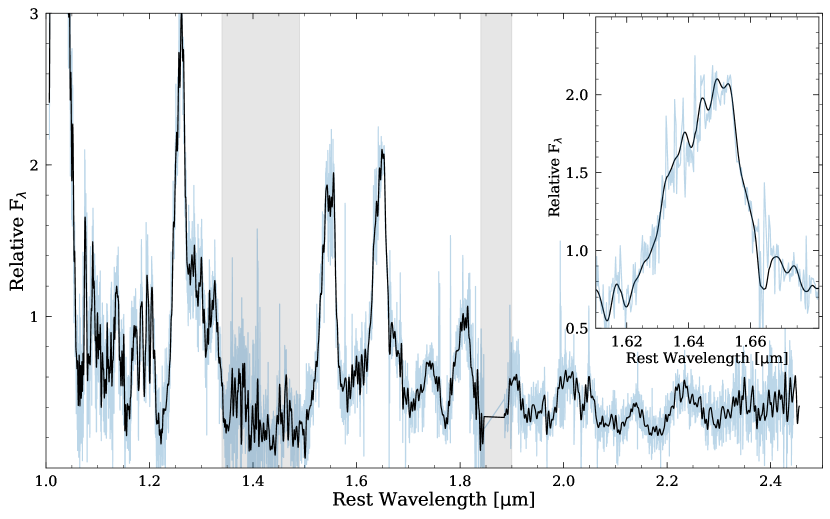
Figure 1: A near-IR spectrum of the peculiar type Ia SN 2020qxp/ASASSN-20jq obtained with the Keck telescope (+NIRES) $+$191 d past the epoch of rest-frame $B$-band maximum. The observed 1-D spectrum is plotted in blue, while the black line corresponds to a smoothed version. The inset highlights the unusual [Fe II] 1.6443 $\micron$ line profile. Shaded areas mark regions affected by the atmosphere. Specific line transitions are listed in Table 2 and features are labeled in Figure 4.

Our paper is organized as follows. In § 2 we present the data. In § 3, the motivation is given for our approach. In § 4, our numerical methods are presented to simulate the nebular phase, and the off-center explosion model for SN 2020qxp/ASASSN-20jq is characterized. In § 5, we provide estimates for the properties of the early synthetic light curve properties. In §6, we develop the methods to analyze the line profiles and synthetic spectra and apply those to the observation of SN 2020qxp/ASASSN-20jq. We next present our final discussion in § 7, followed by our conclusions in § 8.

2 Observations of SN 2020qxp/ASASSN-20jq

SN 2020qxp/ASASSN-20jq was discovered by the All-Sky Automated Survey for Supernovae (ASASSN, Shappee et al. 2014; Kochanek et al. 2017) on 2020 August 8.13 UT in the outskirts of the SBm galaxy NGC 5002. The red-shift of the host galaxy is $z=0.003639$ (Ann et al., 2015). There are several direct distance measurements of NGC 5002, all three using the Tully-Fisher method. Here we adopt the recent Cosmicflows-4 program distance modulus $\mu=31.44\pm 0.43$ mag (Kourkchi et al., 2020). The foreground Milky Way reddening along the line-of-sight of SN 2020qxp/ASASSN-20jq is $E(B-V)_{{\rm MW}}$=0.01 mag (Schlafly & Finkbeiner, 2011), while the host-galaxy reddening is likely small as there is no evidence for significant Na I D in the classification spectrum.

SN 2020qxp/ASASSN-20jq was classified initially as a transitional SN Ia similar to SN 2007on (Stritzinger & Ashall, 2020). Using the classification spectrum, pseudo-equivalent width (pEW) measurements of the Si II$\lambda 5972$ and Si II$\lambda$6355 features place SN 2020qxp/ASASSN-20jq among the cool (CL) SN Ia subtype on the Branch diagram. Furthermore, an initial analysis of an unpublished $B$-band light curve (S. Bose et al., in prep) indicates it reached on 2020 August 23.42 UT (i.e., MJD$59085.43\pm 1.52$) an apparent peak magnitude of $m_{B}=14.74\pm 0.06$ mag. Correcting for Milky Way reddening and assuming the most recently published Tully-Fischer distance, the peak apparent magnitude corresponds to an absolute magnitude of M${}_{B}=-$16.7$\pm$0.4 mag. SN 2020qxp/ASASSN-20jq is indeed a low-luminosity, CL SN Ia.

Our medium-resolution nebular NIR spectrum of SN 2020qxp/ASASSN-20jq was obtained with the Keck-II telescope equipped with the Near-Infrared Echellette Spectrometer (NIRES) on 2021 March 04.5 UT (i.e., MJD=59277.50). This is +191 rest-frame days (d) past the epoch of $B$-band maximum ($t_{B}$). The mean resolution of the spectrum is $R\approx 2700$ and the spectral range extends between $0.96-2.46$ $\micron$. Three sets of ABBA exposures were taken, with each individual A/B exposure of 300 s, yielding a total exposure time on target of 1 hour. The data were reduced following standard procedures described in the IDL package Spextools version 5.0.2 for NIRES (Cushing et al., 2004). The extracted 1-D spectrum was flux calibrated and also corrected for telluric features with Xtellcorr version 5.0.2 for NIRES making use of observations of the A0V standard star HIP65280 (Cushing et al., 2004). As we do not have late-time NIR photometric observations of SN 2020qxp/ASASSN-20jq the absolute flux scale of our spectrum is uncertain. However, the line strengths and relative flux scale is well established due to the reduction method.

The spectrum of SN 2020qxp/ASASSN-20jq is plotted in Fig. 1. Inspection of the data reveals broad emission features ubiquitous to normal SNe Ia at similar epochs. Most interestingly, the single ion [Fe II] 1.644 µm emission feature (Höflich et al., 2004; Diamond et al., 2015), which is highlighted within the figure’s inset, exhibits a very asymmetric profile and contains several novel properties. The 1.644 $\micron$ feature exhibits (going from blue from red) a slanted triangular shape going to the peak, followed by an abrupt drop off in the flux redwards of the peak. The shape of the profile is similar to that observed in the Type Iax SN 2012Z, however, the shape is somewhat different and rather than describing it as a pot-bellied profile (Stritzinger et al., 2015), we refer to it as right-triangle shaped, where the hypotenuse slopes redward. The peak of the feature is located at 1.6545 $\mu$m and is therefore red-shifted from the rest wavelength of 1.644 µm. The top of the feature is tilted over a wavelength range corresponding to about 6,000 $\text{km}~{}\text{s}^{-1}$ in Doppler shift. That is, the small leg of the right triangle has a wavelength extent corresponding to about 6000 $\text{km}~{}\text{s}^{-1}$. Finally, the flux redwards of the peak of the feature plunges rapidly to the pseudo-continuum. In the following, we will refer to the shape of the [Fe II] 1.644 µm feature as a “right-triangle shaped” profile. Similar profiles have previously been produced in the 1.644 [Fe II] µm feature in our published models (Höflich et al., 2004; Penney & Hoeflich, 2014; Diamond et al., 2015), but not with the strong right-triangle shape seen in SN 2020qxp/ASASSN-20jq.

3 Motivation

Comparisons of well observed SNe Ia within the same host galaxy and brightness-decline rates firmly established the diversity in absolute luminosity and spectra for both normal-bright and transitional supernovae (Gall et al., 2018; Burns et al., 2018, 2020). Transitional and sub-luminous SNe Ia are a key to determining which scenario(s) truly exist (Gall et al., 2018; Ashall et al., 2018; Galbany et al., 2019a). However, the interpretation of the differences and specific models are not agreed upon. In the case of the transitional twins SNe 2007on and SNe 2011iv, the difference of the peak-to-tail ratios of the light curves, colors and photospheric spectra have been attributed to different central densities of the WD in a $M_{\rm{Ch}}$ mass explosion (Gall et al., 2018). Alternatively, based on multi-component features in the optical spectra, it has also been suggested that SN 2007on, as opposed to SN 2011iv, resulted from the direct collision of two low mass WDs where both WDs were incinerated (Mazzali et al., 2018). In the case of the sub-luminous SN 2016hnk, based on optical light curves and spectra, this object was attributed to the explosion of a high-density $M_{\rm{Ch}}$ mass WD because a very narrow (500 km s^-1) [Ca II] doublet at $0.7293,7326$ µm was observed on top of a wide [Ca II] feature (Galbany et al., 2019a). An alternative interpretation was a very low mass, $0.85~{}M_{\odot}$, sub-$M_{\rm{Ch}}$ model that also produced the strong and wide component of [Ca II], but questions the existence of the narrow [Ca II] component (Jacobson-Galán et al., 2020). Below, we discuss a mechanism to produce even stronger [Ca II] in underluminous objects like SN 2020qxp/ASASSN-20jq within a $M_{\rm{Ch}}$ scenario. We show why complex spectra during the nebular phase depend sensitively on details of the atomic models, namely non-LTE vs. LTE simulations, and how line profiles add robust diagnostics.

We will use the delayed-detonation scenario of a $M_{\rm{Ch}}$ mass WD because it has predicted many features prior to near- and mid-IR observations (Wheeler et al., 1998; Höflich et al., 2002; Telesco et al., 2015). Moreover, a significant amount of EC elements (e.g. Brachwitz et al., 2000) is commonly detected in X-ray observations of supernova remnants (Badenes et al., 2003, 2006; Thielemann et al., 2018; Ohshiro et al., 2021), and the solar isotopic ⁴⁸Ca/Ca ratio requires burning under conditions found in high-density $M_{Ch}$ WDs (Brachwitz et al., 2000; Thielemann et al., 2018).

Line profiles in the optically-thin nebular phase reveal the asymmetry and burning conditions, and the imprint of the explosion. Commonly, for spectral features in the optical and NIR, multi-component Gaussian fits are employed for efficiency (Graham et al., 2017), at the cost of a large number of free parameters for each spectral feature. Though guided by atomic line lists, fits are mostly unrestricted by the underlying physics. The results, nevertheless, are important as they allow identifying elements and main ionization states as a function of time, and this method provides an estimate of the expansion velocities. Alternatively, highly simplified one-zone models, i.e. constant abundances, ionization and temperature are applied without radiation transport (Flörs et al., 2020) which severely hampers the link to the explosion physics because the structure is unlike that of any SNe explosion. However, it shows the importance and validity of atomic data and that, likely, the ionization balance does not change significantly over the line forming region. Semi-analytical methods are complementary to the progress in complex theoretical models. The latter make use of information from both the physical laws and conservation of, e.g., mass and energy, and observations. Complex models provide a tighter link to the progenitor and explosion physics. Moreover, uncertainties in the underlying physics, e.g., the ionization or atomic data, show up in shortcomings of spectral fits (see §4.1 and 6). Detailed methods include the abundance tomography (Mazzali et al., 2014), or non-LTE models using a direct approach (Kozma & Fransson, 1992; Höflich, 1995a; Jerkstrand et al., 2011; Fransson & Jerkstrand, 2015a; Diamond et al., 2015; Botyánszki & Kasen, 2017a; Blondin et al., 2018; Shingles et al., 2020; Wilk et al., 2020). Therefore, we employ detailed non-LTE model simulations even in multi-dimensional models.

Table 1: Names and properties of our underluminous delayed-detonation models. We give the central density $\rho_{\rm c}$ in $10^{9}$g cm^-3, the location of the DDT ($M_{\rm WD}$ in $M_{\rm Ch}$), the peak brightness $B_{max}$ in magnitudes using the Johnson filter systems (Bessell, 1990), and the luminosity to decline ratio $\Delta m_{15,s}$ in B and V in magnitudes per day. All models have the same main sequence mass, metallicity and transition density $\rho_{\rm tr}$. For the spherical models, the DDT is triggered on a sphere with $\rho_{tr}=1.6\times 10^{7}$ g/cm³ rather than a point. $M_{DDT}$ is given in parenthesis.

Model Name	$\rho_{\text{c}}$	$M_{\text{DDT}}$	$B_{max}$	$\Delta m_{15,s}(B/V)$
5p02822d20.16	2.	(0.24)	$-$18.25	1.69/1.18
5p02822d40.16	4.	(0.25)	$-$17.92	1.42/1.02
Model 00	4.	0.0	$\cdots$	$\cdots$  $\cdots$
Model 03	4.	0.3	$\cdots$	$\cdots$  $\cdots$
Model 09	4.	0.9	$\cdots$	$\cdots$  $\cdots$

4 Models for the Off-center detonations

The analysis in this work is based on the DD scenario, where the basic parameters come from the model-16-series presented by Hoeflich et al. (2017a). This suite of models has also been previously employed in the analysis of the SN remnant S-Andromeda (Fesen et al., 2007, 2015), and for the transitional type Ia SNe 2007on and 2011iv (Gall et al., 2018) which exhibit similar brightness characteristics to SN 2020qxp/ASASSN-20jq. The free parameters in the models are the main sequence mass, $M_{\rm MS}$, metallicity $Z$ of the initial WD, its central density, $\rho_{c}$, at the time of the explosion, the transition density, $\rho_{{\rm tr}}$, and the location of DDT in mass coordinate $M_{DDT}$. All delayed-detonation models have $M_{MS}=5$ $M_{\odot}$, $Z=Z_{\odot}$, and $\rho_{{\rm tr}}=1.6\times 10^{7}$ g cm^-3. We increased $\rho_{\rm c}$ by a factor of two (i.e., $\rho_{\rm c}=4\times 10^{9}$ g cm^-3) in order to reproduce the right-triangle shaped profile of the 1.644 µm feature, namely to produce the ‘flat’ (linear slope of the central profile) property with the ‘tilt’ being a result of the off-center DDT as discussed in § 6.1, but keep the other basic parameters fixed. Our goal is not to produce a specifically tuned model, just to reproduce the overall NIR spectrum of SN 2020qxp/ASASSN-20jq.

Following the convention adopted by Domínguez & Höflich (2000); Höflich et al. (2002), the spherical delayed-detonation models are referred to as 5p02822dXX.16 with XX specifying $\rho_{\rm c}$ in $10^{8}$g cm^-3.

The synthetic spectra are calculated at 210 days after the explosion, which is consistent with $191\pm 4.3$ days past the observed $B$ maximum for SN 2020qxp/ASASSN-20jq (see § 2 & § 5).

In the following, aspherical models are referred to as “Model YY” with YY denoting the position of the DDT being the offset in units of $1/10^{th}$ of the total mass. Note that Model 00 has free parameters identical to the spherical model 5p02822d40.16 but, for consistency, it was simulated on the 3D grid. The set of models is shown in Table 1.

4.1 Numerical Methods

Our models are based on full multi-dimensional hydro and non-LTE simulations applied to the nebular phase in SNe. We mention the basic methods, discuss the requirements dictated by the physical conditions, and explain the limitations.

The simulations utilized in this work are computed using the HYDrodynamical RAdiation code (HYDRA) that consists of physics-based modules which provide solutions for: the rate equations that determine the nuclear reactions, the statistical equations needed to determine the atomic level populations, the equation-of-state, the matter opacities, the hydrodynamic evolution, and the radiation-transport equations (RTE). The RTE is treated by solving the co-moving frame equations in spherical geometry or using Variable Eddington Tensor methods, with a Monte-Carlo (MC) scheme providing the necessary closure relation to the momentum equations needed to solve the generalized scattering and non-LTE problem. An MC approach is used for the transport of $\gamma$-rays and positrons and for calculating the emergent spectra (Hoeflich, 1990; Höflich, 1995a, 2003, 2009; Penney & Hoeflich, 2014; Hristov et al., 2021). RTE is needed because most of the SN envelope is still optically thick in the UV (and with significant optical depth in $U$ and $B$) during the nebular phase, which affects the lower levels via bound-free and allowed bound-bound transitions and, thus, the ionization balance via the incomplete Rosseland cycle, and the excitation of higher levels.

In these simulations for the early phase, the hydrodynamical equations are solved using an explicit Piecewise Parabolic Method (PPM) without adaptive mesh refinement (Colella & Woodward, 1984; Fryxell, 2001; Fryxell et al., 1991), followed by a phase of free expansion of the envelope (Hoeflich et al., 2017b).

A nuclear reaction network is used with rates for weak, strong and electromagnetic reactions. The nuclear reaction network is based on the implementation of Thielemann et al. (1994a, b), but with updated cross-sections published in Cyburt et al. (2010). For this study, the reduction of the new EC rates by factors up to 5 (e.g. Thielemann et al., 1994a; Langanke et al., 2004) compared to the old values is important, as it changes the production of EC-elements. This is reflected in the transition from ‘flat-topped’ (Höflich et al., 2004) to ‘pot-bellied’ profiles (Höflich et al., 2004; Motohara et al., 2006; Maeda et al., 2011; Stritzinger et al., 2015; Diamond et al., 2015; Gall et al., 2018). The revised cross-sections enter directly our estimates of the initial central density required (§ 6).

Detailed atomic models are used for the ionization stages I-IV for C, O, Ne, Mg, Si, S, Cl, Ar, Ca, Sc, Ti, V, Cr, Mn, Fe, Co, Ni. The atomic models and line lists are based on the database for bound-bound transitions of van Hoof (2018), supplemented by additional forbidden lines from Diamond et al. (2015). Note that the atomic levels are based on levels both with and without known transition probabilities because collisions are crucial to avoid the IR catastrophe (Axelrod, 1980a; Fransson & Sonneborn, 1994), and because of its apparent absence in observations. This is important to simulate the effective critical density because, in our $M_{Ch}$ mass explosions, the densities at 210 days past the explosion are $\approx 10^{7}$ particles cm^-3 in the region of EC elements.

Though we do not merge fine-structure levels related to the 1.644 µm  feature (Penney & Hoeflich, 2014; Diamond et al., 2015), the use of superlevels, i.e. the merging of some atomic fine-structure levels, tends to overestimate emission from the excited levels within multiplets of iron-group elements (§ 6.2). We assume the radioactive decay by ⁵⁶Ni $\rightarrow^{56}$Co $\rightarrow^{56}$Fe. The energy deposition by hard $\gamma$-rays and non-thermal electrons and positrons enters the rate equations via non-thermal ionization balanced by the recombination processes similar to Kozma & Fransson (1992), under the assumption that the local nuclear energy input per time is balanced by the local flux (Höflich et al., 1992, 2004; Penney & Hoeflich, 2014; Hristov et al., 2021). For a summary and some discussion of the ionization structure, see Appendix A.

The multi-dimensional non-LTE simulations presented in this paper are limited in resolution. The overall model spectra are low resolution ($R=150-300$) because memory requirements for the hydro, radiation transport, and non-LTE atoms limits the resolution currently possible in HYDRA. 3-D models use (330x70x70) as spatial grid ($r,\Theta,\phi$) and $\approx 6,000$ energy bins for the radiation field. The atomic rate equations are solved on ($330\times 70$) spatial cells using the overall symmetry of the problem discussed in this paper. For the emergent spectra, we use up to 10,000 frequency counters in the observer’s frame in 21 directions.

During the nebular phase, the optical and IR flux is predominately produced by forbidden transitions in the semi-transparent regime and the emissivity is dominated by spontaneous emission providing stability of the solution of the full RTE problem (the solution of the radiative transfer equation, the solution of the rate equations, and conservation of energy) and of the robustness of the spectra. In particular, the forbidden unblended [Fe II] at 1.644 µm line is formed in Fe dominated layers which show rather small variations in the ionization balance. Moreover, being unblended minimizes radiative coupling in an expanding envelope. Combined, this leads to the stability of the resulting line profile as a probe of geometry for features dominated by single transitions. Note that the agreement between the line strenghts of different ions is generally good (see §6.2) which might indicate that the predicted ionization and excitation states are close to correct. However, atomic data and even some level energies (Friesen et al., 2017; Diamond et al., 2018) are a major uncertainty to reproduce complex profiles of features formed by multiple lines, as discussed in § 6.

4.2 Model Setup

In constructing off-center delayed-detonation models, we have followed the prescription of Livne (1999), also the approach utilized by Fesen et al. (2015). We limited the deflagration burning to 0.95 of the fuel to allow for the detonation front traveling through the core to bring our results in close agreement with those of Gamezo et al. (2005) and Fesen et al. (2015). In this prescription, the initial deflagration phase is modeled assuming spherical symmetry. The deflagration begins at the center and propagates outward in a subsonic deflagration front. The energy deposited by deflagration causes the entire WD to expand with a velocity of $\sim 2,000-3,000$ $\text{km}~{}\text{s}^{-1}$ (Hoeflich, 2017). When the density at the leading edge of the deflagration wave has fallen to the transition density $\rho_{tr}$, a detonation is ignited by hand at a single point (the north pole) of the deflagration front, imposing rotational symmetry.

Within the off-center delayed-detonation models, abundance asymmetry is produced because the DDT occurs on the background of an already expanding envelope. The final outcome of the density structure is close to spherical because the detonation occurs in the density structure of a quasi-static WD. After the DDT, a weak detonation front propagates through the WD at close to the speed of sound. Close to the time of the transition, burning occurs under higher density than other layers at the same distance from the center because the detonation reaches those later. Subsequently, the hot WD accelerates into free expansion, and the stored thermal energy is converted into kinetic energy. The resulting density structure is close to spherical because the specific kinetic energy hardly depends on whether burning continues to nuclear statistical equilibrium (NSE) or quasi-statistical equilibrium (QSE) as also suggested by the full 3D simulation of Gamezo et al. (2005). The final abundance profiles of Model 03 are shown in Fig. 2.

We impose spherical symmetry on the initial deflagration phase for two reasons: (i) computational tractability, 3-dimensional simulations are computationally expensive, requiring many $10^{5}$ CPU hours, e.g. (Khokhlov & Höflich, 2001; Röpke et al., 2003; Gamezo et al., 2003, 2005; Plewa, 2007; Röpke et al., 2007; Hristov et al., 2021); (ii) pure hydrodynamical multi-dimensional simulations predict mixed chemical profiles, which are at odds with observations of typical SNe Ia. Observations strongly suggest the existence of a process that partially suppresses the dominant role of Rayleigh-Taylor (RT) instabilities, despite evidence for structures on the scale of RT instabilities. These observations include: post-maximum spectra in normal-bright and sub-luminous SNe Ia (Wheeler et al., 1998; Höflich et al., 2002; Ashall et al., 2019); line profiles in many SNe Ia $1-2$ years after the explosion, which indicate stable isotopes near the center after the initial phase of burning (Maeda et al., 2011; Höflich et al., 2004; Motohara et al., 2006; Maeda et al., 2010, 2011; Stritzinger et al., 2014; Diamond et al., 2015; Friesen et al., 2017; Diamond et al., 2018); direct imaging of S-Andromeda which shows a Ca-free core (Fesen et al., 2007). Recently, high-resolution spectropolarimetry obtained by the VLT (Patat, 2005; Yang et al., 2020) shows indications of chemical plumes on the scale of RT instabilities but limited to specific layers in the WD.

The actual origin of this partial suppression of RT instabilities is not known; however, recent 3D simulations of the flame demonstrate the influence of high magnetic fields on the deflagration fronts and the partial suppression of RT instabilities (Remming & Khokhlov, 2014; Hristov et al., 2018), suggesting a possible physical mechanism to suppress strong mixing material induced by RT instabilities. The presence of high magnetic fields has been inferred from the lack of positron transport effects in late-time NIR line profiles and light curves which show decline rates that never fall below the ⁵⁶Co decay lines (Cappellaro et al., 1997; Stritzinger et al., 2002; Höflich et al., 2004; Penney & Hoeflich, 2014; Kerzendorf & Sim, 2014; Diamond et al., 2015; Graur et al., 2017; Shappee et al., 2017; Diamond et al., 2018; Yang et al., 2018; Hristov et al., 2021).

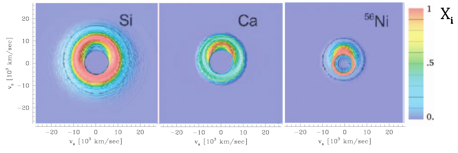
Figure 2: Distribution of elements in spherical geometry (upper) for our underluminous models with $\rho_{c}=4\times 10^{9}$ g cm^-3 leading to a region of EC elements of $\approx 3,000$ km s^-1 similar to SN 2016hnk (Galbany et al., 2019b). In the lower panels, we give the distribution of Si, Ca and ⁵⁶Ni for the off-center DDT at $0.3$ $M_{{\rm WD}}$ in velocity coordinates. The abundances are given in mass fractions $X_{i}$ and are color coded in a domain size of $\pm 27,500$ $\text{km}~{}\text{s}^{-1}$. The inner EC region is spherical as it is produced during the deflagration burning phase and shows the same abundances as in the spherical model. Without mixing, the size of the EC region shrinks to $\approx 1,500$ and $\approx 500$ km s^-1 for $\rho_{c}$ of $2\times 10^{9}$ g cm^-3 and $1\times 10^{9}$ g cm^-3, respectively (see Diamond et al., 2015, their Fig. 4).

5 Light Curve Parameters

The early light curve has been calculated for the spherical model 5p02822d40.16 with increased central density to $\rho_{c}=4\times 10^{9}$ g cm^-3. Using the Johnson filter system (Bessell, 1990), the light curve values for our high-density version, model 5p02822d40.16, are $M_{B}=-17.92$ mag, $B(t_{B})-V(t_{B})=0.08$ mag with a rise time $t_{B}=16.9~{}d$, $dm_{15,B}=1.42$, $dm_{15,V}=1.02$ mag respectively for the spherical model, compared to, with no host reddening correction, $M_{B}=-16.7\pm$0.43 mag for SN 2020qxp/ASASSN-20jq (see § 2). Note that, compared to 5p02822d20.16 with the lower $\rho_{\rm c}$, the high-density model is dimmer, the rise time is shorter and the decline is less steep (see Tab. 1) because of the lack of energy deposition close to the center at early times, resulting in shorter diffusion timescales and less energy being stored before maximum light. Moreover, there is significant uncertainty due to asphericity effects. We did not calculate the time-dependent 3D models during the photospheric phase. The aspherical Model 03 seen from $-90^{o}$ will be dimmer because it is observed from the opposite side of the ⁵⁶Ni-bulge which is hidden during the photospheric phase (see Fig. 2). Stationary scattering models give a factor $\approx 2$ in luminosity (see Höflich (1995b) in their Fig. 2, left plots). We note that the fluxes and properties of the outer layers are very sensitive to small variations in the transition density $\rho_{tr}$ in the regime of low-luminosity SNe Ia whereas the inner layers depend mostly on $\rho_{c}$ (Höflich et al., 2002; Hoeflich et al., 2017a). In light of the high asymmetry inferred below, fine-tuning of the model parameters has not been performed, nor is it necessary. The early lightcurve properties from spherical non-LTE simulations should be regarded as indicative for this class of models. The full 3D non-LTE lightcurves and spectra during the photospheric phase are currently prohibitively expensive in both CPU and memory requirements.

6 Analysis and Interpretation of Line profiles and spectra

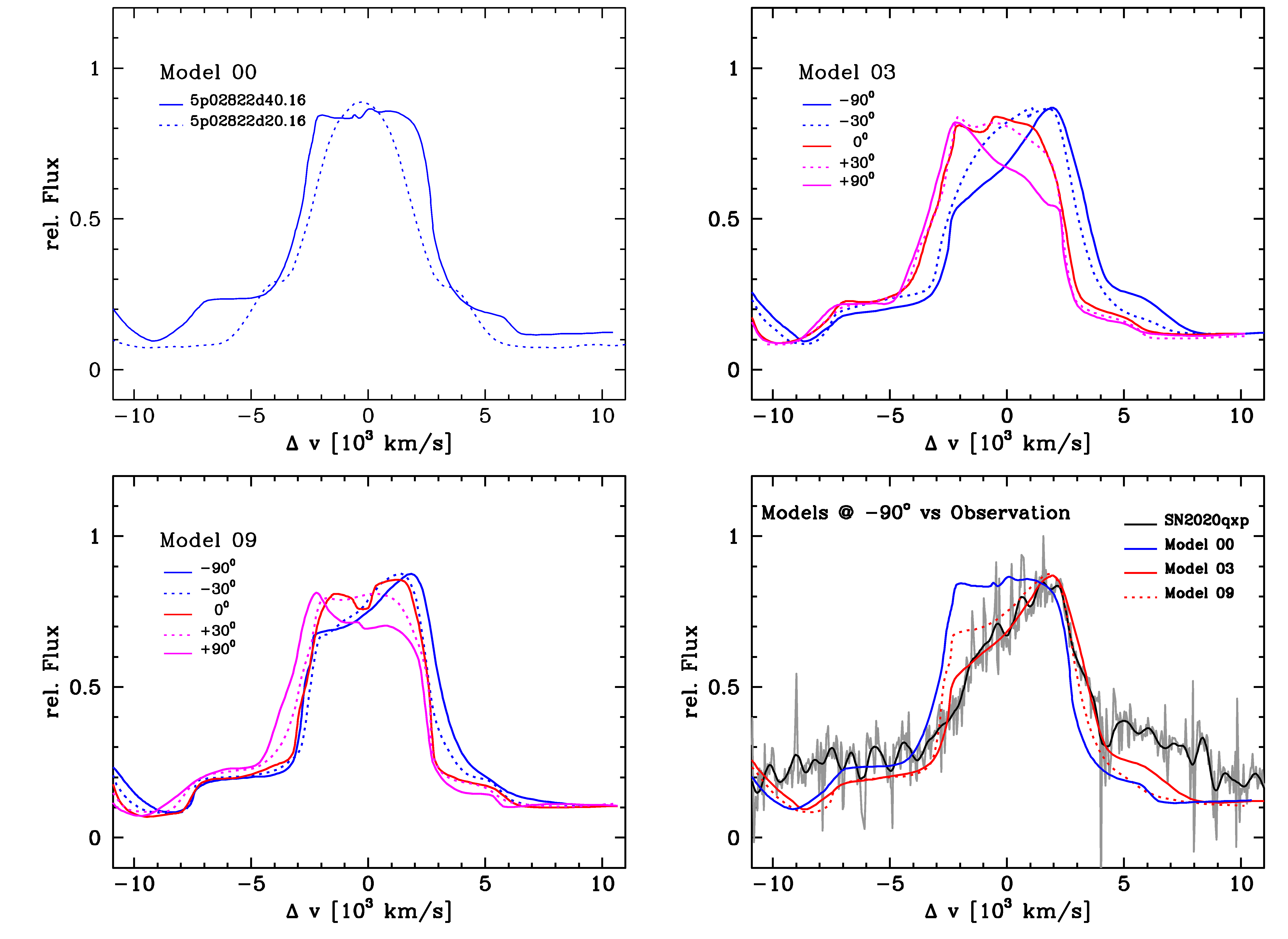
Figure 3: Directional dependence of the synthetic line profiles for off-center delayed-detonation models (upper and lower left), and the comparison with SN 2020qxp/ASASSN-20jq to identify the optimal location of the DDT (lower right). The line profile of the minimally blended feature produced by the forbidden [Fe II] at 1.644 µm at about 210 days after the explosion is shown for our off-center delayed-detonation models seen from various directions, and SN 2020qxp/ASASSN-20jq. The observation has been blue-shifted by $500~{}\text{km}~{}\text{s}^{-1}$ to be aligned with the red wing and the center of the flat portion with the kinematic center of Model 03. The flux peaks at $2,000~{}\text{km}~{}\text{s}^{-1}$. No zero-point adjustments has been applied to the observation, though a 10 % shift would be compatible with the noise in the data, and improve the fit in the wings beyond $\pm 5,000~{}\text{km}~{}\text{s}^{-1}$. The synthetic spectra are based on our underluminous explosion models with a central density of $\rho_{c}=4\times 10^{9}$ g cm^-3 with ignition points for the delayed-detonation transitions in mass coordinates at 0., 0.3 and 0.9 $M_{\rm{Ch}}$, Model 00 plus the low-density version with $\rho_{c}=2\times 10^{9}$ g cm^-3 (upper left), 03 (upper right) and 09 (lower left). For a discussion, see § 6.1. Note that the total width of the synthetic emission component is wider than observed by $\approx 650$ km s^-1. This can be attributed to the much better resolution of the spectrograph ($\bar{R}=2700$) compared to the effective resolution $R\approx 300$ of the theoretical model (see § 4.1).

Table 2: List of forbidden lines that significantly contribute to the synthetic spectral flux. For each transition, the markers correspond to strong ($***$), moderate ($**$), weak ($*$), and scarcely detectable ( ) on top of the quasi-continuum formed by a large number of lines. The relative strength S is estimated by the integral over the envelope, $\int{A_{ij}\times n_{j}~{}dV}$ with $n_{j}$ being the particle density of the upper level. We give the rest wavelength in $\mu$m, and identify the ion. All spectral features are strongly blended with the exception of that due to [Fe II] at $1.644$ µm because the Doppler shift smears out each transition by about $3\%$. Note that transitions are ordered with increasing wavelength from left to right.

S   $\lambda$[µm ]	Ion	S    $\lambda$[µm ]	Ion	S    $\lambda$[µm ]	Ion	S    $\lambda$[µm ]	Ion	S    $\lambda$[µm ]	Ion
$**$ .9952	[Fe II]	$***$ .9959	[Ni II]	.9962	[Fe III]	1.000	[Fe I]	$**$ 1.001	[Fe II]
$**$ 1.004	[Fe II]	$**$ 1.013	[Fe II]	$**$ 1.019	[Co II]	$**$ 1.021	[Ni II]	1.023	[Fe I]
$***$ 1.024	[Co II]	1.026	[Fe I]	$***$ 1.028	[Co II]	$**$ 1.029	[Si II]	$**$ 1.032	[Si II]
$*$ 1.032	[Si II]	$**$ 1.034	[Si II]	$*$ 1.037	[Si II]	$*$ 1.043	[Fe II]	$**$ 1.046	[Ni II]
$*$ 1.057	[Fe II]	$*$ 1.064	[Ni II]	$***$ 1.071	[Ni II]	$**$ 1.082	[Si I]	$**$ 1.089	[Fe II]
$*$ 1.092	[Ni II]	$**$ 1.099	[Si I]	$**$ 1.104	[Fe II]	1.106	[Co III]	$**$ 1.116	[Fe II]
$**$ 1.131	[Si I]	$*$ 1.135	[Co III]	$*$ 1.135	[Fe II]	$**$ 1.136	[Ni II]	$*$ 1.146	[Ni II]
$*$ 1.154	[Si I]	$**$ 1.161	[Ni II]	1.187	[Co III]	$**$ 1.191	[Fe II]	$**$ 1.205	[Fe II]
$*$ 1.223	[Fe II]	$**$ 1.232	[Ni II]	$*$ 1.248	[Fe II]	$**$ 1.249	[Fe II]	$**$ 1.25	[Fe II]
$*$ 1.252	[Fe II]	$***$ 1.257	[Fe II]	$***$ 1.271	[Fe II]	$*$ 1.273	[Co III]	$*$ 1.278	[Ni II]
$***$ 1.279	[Fe II]	1.293	[Ni II]	$***$ 1.294	[Fe II]	$**$ 1.298	[Fe II]	$*$ 1.310	[Co III]
$***$ 1.321	[Fe II]	1.321	[Fe I]	$***$ 1.328	[Fe II]	1.335	[Ni II]	$*$ 1.339	[Ni II]
1.342	[Fe I]	$*$ 1.356	[Fe I]	$*$ 1.368	[Fe I]	$***$ 1.372	[Fe II]	$*$ 1.373	[Fe I]
1.3746	[Fe I]	$*$ 1.443	[Fe I]	$**$ 1.484	[Fe II]	$**$ 1.491	[Fe II]	$**$ 1.525	[Fe II]
$***$ 1.534	[Fe II]	$**$ 1.547	[Co II]	$***$ 1.549	[Co III]	1.588	[Si I]	$***$ 1.600	[Fe II]
$*$ 1.607	[Si I]	$***$ 1.644	[Fe II]	$*$ 1.646	[Si I]	1.646	[Si I]	$**$ 1.664	[Fe II]
$*$ 1.677	[Ni II]	$***$ 1.677	[Fe II]	$**$ 1.712	[Fe II]	$*$ 1.725	[Ni II]	$*$ 1.741	[Co III]
$**$ 1.745	[Fe II]	$*$ 1.764	[Co III]	$**$ 1.765	[Ni II]	$**$ 1.798	[Fe II]	$**$ 1.801	[Fe II]
$*$ 1.803	[Fe II]	$**$ 1.810	[Fe II]	$**$ 1.812	[Fe II]	$*$ 1.814	[Fe II]	1.821	[Co III]
$*$ 1.844	[Mn II]	$*$ 1.914	[Fe II]	$**$ 1.939	[Ni II]	$*$ 1.958	[Co III]	$**$ 1.967	[Fe II]
1.969	[Fe III]	$*$ 2.002	[Co III]	$*$ 2.003	[Fe II]	$***$ 2.007	[Fe II]	2.022	[Fe III]
$***$ 2.047	[Fe II]	$**$ 2.049	[Ni II]	$*$ 2.072	[Fe II]	$*$ 2.081	[Ni II]	$*$ 2.086	[Fe II]
$*$ 2.098	[Co III]	$*$ 2.102	[Ni II]	$**$ 2.133	[Fe II]	2.146	[Fe III]	$*$ 2.219	[Fe III]
2.243	[Fe III]	$***$ 2.244	[Fe II]	$**$ 2.267	[Fe II]	$*$ 2.281	[Co III]	$**$ 2.309	[Ni II]
$*$ 2.335	[Ni II]	2.349	[Fe III]	$*$ 2.361	[Ni II]	$**$ 2.369	[Ni II]	$**$ 2.371	[Fe II]

Figure 4: Comparison of the synthetic spectrum for the spherical (red) and aspherical model 03 seen from $-90^{o}$ (blue dashed, $R\approx 250$) with the NIR Keck spectrum of SN 2020qxp/ASASSN-20jq from 03/04/2021. As an inset, the synthetic optical spectrum is given normalized to the photometric B-band. The spectrum is dominated by blends of forbidden lines of singly and doubly ionized Fe, Co and Ni, and a weak [Ni II]/[Fe II] blend at about 1.9 microns (see Table 2). The three strongest NIR & the Ni feature are labeled with the main (black) and secondary (gray) contributing ions. Note that the strong features at $1.25$ and $1.55~{}\mu$m have shapes caused by blends of more than 15 and 7 transitions, respectively, rather than revealing any underlying asymmetries. The [Ni II] feature at $1.9~{}\mu$m is flat-topped. The strengths of features are hardly affected by asphericity but Model 03 produces Doppler shifts of the peak fluxes which closely match the observations. For a discussion including the optical [Ca II] feature at 0.73 $\mu$m, see §  6.2, and identifications for the strongest optical transitions are given in the appendix. Though observed and theoretical features are consistent in between 1.38-1.44 and 1.81-1.93 $\mu$m (shaded in light gray), those telluric regions are impacted in the observations (see also Fig. 1).

We use the $1.644$ µm feature of SN 2020qxp/ASASSN-20jq  to find parameters for the central density of the WD, the off-center position of the DDT, and the inclination angle. Subsequently, we compare the entire NIR spectrum with these parameters for verification and further analyses.

Figure 5: Same as Fig. 4 but with the blown up spectral regions of the $1.25$ µm (consisting of many [Fe II] blends) feature, $1.55$ µm (dominated by two [Co III] and [Fe II] transitions) feature and, as an inset, the $1.9$ µm feature which is dominated by [Ni II] and weaker [Fe II] transitions (see Table 2). The peaks are better reproduced by Model 03. Model 00 tilts the $1.25$ and $1.55$ µm profiles in opposite direction compared to the observations, and is not a good fit. Neither of these features is dominated by the asymmetry. The ⁵⁸Ni feature is flat topped and offset (see §6.1). Note that the impact of differences in resolution between observation and synthetic spectrum, and uncertainties related to the atomic models (too strong emission in the red wings from excited fine-structure levels within a multiplet) when describing complex features (see §4.1 & 6.2). The $1.55$ µm double-horn profiles produced by [Co III] and [Fe II] (Table 2) are seen in our high resolution simulations ($R\gtrsim 1,000$ Penney & Hoeflich, 2014; Diamond et al., 2015, and the observation $R=2,700$), but are merged due to the low $R_{\text{eff}}\sim 500$ in our 3D simulations.

6.1 Profile of the 1.644 micron Feature

This line profile can be understood by the abundance distribution. In Fig. 3, the profiles of the $1.644$ µm feature are shown for Models 00, 03 and 09, and compared to the profile of SN 2020qxp/ASASSN-20jq. The overall profiles are characterized by an almost unblended central region with blue and red shoulders due to the components of weak [Fe II] blends at wavelength shifts corresponding to $\approx-6,000$ and $\approx+5,000$ $\text{km}~{}\text{s}^{-1}$ (Höflich et al., 2004; Diamond et al., 2015).

We first discuss the model with a central DDT that produces a spherical chemical distribution (Fig. 3, upper left). As can be seen, the synthetic profile is ‘flat-topped’ similar to our old model with $\rho_{c}=2\times 10^{9}$ g cm^-3 (Höflich et al., 2004). As discussed in §4.1, the reduction of the EC rates in 2006 combined with lower $\rho_{c}$ $\approx 0.5-2\times 10^{9}$ g cm^-3, typically found in SNe Ia, caused peaked profiles (Hoeflich, 2006; Penney & Hoeflich, 2014; Diamond et al., 2015, 2018). To produce a flat top with low EC rates, we now require a higher $\rho_{c}$ by a factor of $\gtrsim 2$. The extent of the flat top can be used to estimate the size of the ⁵⁶Ni-free region in velocity space and requires $\rho_{c}=4\times 10^{9}$ g cm^-3.

The 1.644 $\mu$m profile of the spherical model does not show a fully symmetric emission component, namely the wings at about $\pm 5,000$ $\text{km}~{}\text{s}^{-1}$ are due to well known blends of weak [Fe II] and [Co III] transitions (Höflich et al., 2004; Diamond et al., 2015). For our model, [Si I] contributes to the underlying continuum flux between $\approx-8000$ to $9000$ $\text{km}~{}\text{s}^{-1}$ basically adding to the flux a broad quasi-continuum contribution.

Another characteristic is the lack of emission at the ‘red’ edge of the flat plateau. It is produced in the models because the envelope is not fully optically thin. At day 210 past the explosion, the photosphere is at about $1,000$ to $1,500$ $\text{km}~{}\text{s}^{-1}$ in the IR, formed by a quasi-continuum of overlapping allowed lines, Thomson scattering, and free-free emission, effectively blocking the light from parts of the redshifted ejecta. At this epoch, our model is making the transition from the photospheric to the nebular phase.

Similarly, the off-center Models 03 and 09 can be understood based on the asymmetric distribution of ⁵⁶Ni (Fig. 2, lower right). Asymmetry introduces a tilt of the flat top (Fig. 3, upper and lower left). Obviously, the profile depends on the direction to the observer. Seen from the equator, the profiles are rather similar to Model 00. Seen from the north and south pole, the ⁵⁶Ni produced during the detonation adds a blue and red-shifted component, respectively. The length of the plateau in velocity space remains almost the same, but the overall profiles are tilted. Note that the peak flux is shifted by $\approx 2,000$ $\text{km}~{}\text{s}^{-1}$. For intermediate angles (i.e. $-30^{o},~{}0^{o},~{}30^{o}$), the profiles shift smoothly between the two extreme cases.

The observed profile of SN 2020qxp/ASASSN-20jq shows a flat-tilted (right-triangle shaped) profile, that is highly asymmetric. The tilt shifts the maximum flux towards the red, suggesting that SN 2020qxp/ASASSN-20jq is observed from the south pole (i.e. the side opposite to the DDT point). The comparison with Models 00, 03, and 09 (Fig. 3, lower right plot) shows good agreement between the observed spectrum and Model 03 seen from an angle of $-90^{o}$ (Fig. 3, lower right).

6.2 The overall NIR (and optical) spectrum

The synthetic and observed spectra of SN 2020qxp/ASASSN-20jq are compared in Fig. 4. We use relative fluxes due to the absolute flux uncertainties in both the observation and model. In case of the observation, the distance is uncertain by about $0.43$ mag (see §2), and no IR photometry are available to accurate flux calibrate the spectrum. On the other hand, in the case of the models the absolute IR flux may change by small adjustments in the ⁵⁶Ni mass which may be needed to reproduce the early spectra, and in addition, would change the typical ratio between the second and third ionization-state. The overall synthetic flux distribution seems to be somewhat steeper from the blue to the red compared to the observation, but the agreement of line strengths of different ions is generally good. The contributions of individual transitions are identified in Table 2. The strongest and most of the medium strong features can be reproduced, namely at $1.04,1.27,1.55,1.644,1.8,1.9,2.07,2.27$ µm. The features are mostly produced by blends of singly and doubly ionized Fe and Co lines within $\approx\pm 2\%$ in wavelength of the peak given. The feature at 1.2 µm can be attributed to fluorescence of [Fe II] emission by neutral Fe (Wilk et al., 2018; Shingles et al., 2020).

The line profiles of the strong 1.27, 1.55 µm features are clearly asymmetric even in Model 00 because of blending between [Fe II]–[Fe III] and [Co II]–[Co III] lines (see Fig. 5 and Table 2). For example, the tilt of the $1.25$ µm feature shows a steep blue and flat red decline produced mostly by multiple blends of some 30+ transitions dominated by [Fe II], whereas the opposite is true for the $1.55$ µm feature which is dominated by two [Co III] and [Fe II] transitions. As shown by Penney & Hoeflich (2014) and Diamond et al. (2015), the time evolution of the feature at $1.55$ µm can be understood by the ⁵⁶Co$\rightarrow^{56}$Fe decay. This, in principle, enables us to separate the effects of blends and of the asymmetric envelope on the resulting profile. In practice, the separation of time and asymmetry effects may be challenging and requires good resolution and high S/N observations.

One feature can be seen at $1.9$ µm in the synthetic spectra and tentatively seen in the observed spectra, although it is in the telluric region. In the model, it can be attributed to [Ni II] and previously has been identified in normal bright SNe Ia by Friesen et al. (2017). In our models this feature is rather weak despite the significant amount of EC $\approx 0.08M_{\odot}$ in the models because high densities in the central region suppress forbidden lines and the photosphere has not yet receded to the center (see § 4.1). The overall feature is blue-shifted and ‘stubby’ without a red-shifted peak because, in our model, the EC distribution is rather spherical. As evident from Table 2, [Ni II] transitions contribute significantly to the emission, but as blends. Note that the strength of the feature depends on collisional de-excitation.

Some features in the synthetic spectra are present but too weak compared to the observation, e.g. in the region at $1.4$ and $2.15$ µm. From the models, emissions may be attributed to multiple transitions of [Fe II] or, in the latter case, to [Ni II] and [Fe II]. In principle, higher ionization to [Fe III] may help because this ion has lines at the corresponding wavelengths, in particular, the [Fe III] 3H-3G transitions at $2.144$ and $2.146$ µm. However, in our models, this would decrease the $1.644$ µm [Fe II] relative to the Fe/Co blend at $1.55$ µm. The discrepancy between models and observations points towards missing cross-sections as a potential problem: some 50% of all [Fe II-Fe III] and [Co II-Co III] transitions have non-measured cross-sections (see § 4.1), a problem not unique to our models (Friesen et al., 2017). Another uncertainty may be the lack of collision rates which suppress forbidden lines at higher excitation levels, or may boost allowed transitions which are known to be important to reproduce spectra in this wavelength range at earlier times in both normal bright and sub-luminous SNe Ia (Wheeler et al., 1998; Höflich et al., 2002; Friesen et al., 2017).

The optical spectrum of Models 00 and 03 is shown as an inset in Fig. 4. It is dominated by singly and doubly ionized Fe/Co and C I, O I, and S I-II. The very prominent feature is the [Ca II] doublet at $0.729,0.732$ µm blended with [Fe II], [Ni II] and [Co II]. In our models, the feature is expected to shoot up between 100 and 200 days after the explosion when the densities in the corresponding Ca-rich layers (Fig. 2) drop below the critical density of our atomic models (see § 4.1). [Ca II] is strong in our model due to the strong overlap of Ca and ⁵⁶Ni produced during the detonation. The total mass of ⁵⁶Ni produced is smaller by a factor of about two compared with normal-bright SNe Ia which show only a very limited overlap between Ca and ⁵⁶Ni and, thus, much weaker [Ca II].

The difference between the profile of the spherical and off-center models suggests [Ca II] as a new diagnostic to probe asymmetries (see inset of Fig. 4): In the spherical case, the feature is broad because the Ca exists in a ring from $\approx-7,000$ to $+7,000$ $\text{km}~{}\text{s}^{-1}$. For an observer, the Ca-rich region spans a wide velocity range from red to blue-shifted segments (Fig. 2, upper figure). Strong asymmetries will produce narrow [Ca II] features, allowing the appearance of the blends mentioned above (Fig. 3). The profile of Model 03 is similar in height, but much narrower than in the spherical model because Ca is only strong in a specific segment of the envelope rather than a sphere (Fig. 2, lower middle plot). If seen from the north pole, the Ca-rich region comes towards the observer, but the red-shifted component is missing, and vice versa if seen from the south pole. The width of the [Ca II] component depends strongly on the direction to the observer. The projected velocities of Ca can be directly read off from Fig. 2 (lower middle plot). From $-90^{o}$ the contribution has a mean half width is $\approx 2,500$ $\text{km}~{}\text{s}^{-1}$, but goes down to $\approx 1,000$ $\text{km}~{}\text{s}^{-1}$ if observed from the equator.

7 Final Discussion

Here, we want to put our detailed analysis of the IR spectrum obtained for SN 2020qxp/ASASSN-20jq into connection with the explosion and progenitor and discuss the results in context of various other leading scenarios.

7.1 Delayed-Detonation Models with an Off-Center DDT

SN 2020qxp/ASASSN-20jq shows a highly asymmetric [Fe II] $1.644$ µm NIR line profile. This profile is reproduced using a full non-LTE 3D modeling code for an SN Ia within the framework of off-center delayed-detonation models.

The distinguishing components of the NIR [Fe II] feature at $1.644$ µm are flat (with no curvature), but right-triangle shaped profiles, which includes a steeply declining component. In addition, there are extended wings due to weak blends of singly and doubly ionized Fe and Co, respectively. The extent of the hypotenuse of the right-triangle shaped profile does not depend on the location of the off-center detonation, and can be used to determine the extent of the inner ⁵⁶Ni-free region. The tilt of the hypotenuse is an effective tool to constrain the angle between the symmetry axis and the observer (see § 6.1, and Figs. 4 $\&$ 3).

The asymmetric profile of SN 2020qxp/ASASSN-20jq can be understood within the framework of delayed-detonation models with a high central density and a DDT triggered in the regime of distributed burning consistent with the Zeldovich mechanism. The DDT occurs on an already expanding background resulting in asymmetric abundance distributions because, for the same mass coordinate in the WD, burning happens at different densities (see § 4).

The high S/N spectrum of the [Fe II] $1.644$ µm feature enables us to separate asymmetry from peculiar velocities (see § 6.1). We show that the shift of the peak flux of $\approx 2,000$ $\text{km}~{}\text{s}^{-1}$ can be mostly attributed to the asymmetry in the explosion rather than a Doppler shift reflecting the motion in the progenitor system, or in the host galaxy. The offset of $\approx-500$ km s^-1 is based on the steep red wing and the center of the short leg of the right-triangle shaped profile. The latter offset is consistent with other NIR features pointing to a kinematic offset, i.e. orbital velocities.

We showed that the overall observed and theoretical NIR spectra agree within uncertainties expected from atomic physics (see § 4.1). We verify that the off-center delayed-detonation model seen from the south pole can reproduce the spectra of SN 2020qxp/ASASSN-20jq. It is shown that the strength of the features hardly depends on the off-centerness of the features (see Fig. 4), but the profiles do (see Fig. 5.)

We weakly suggest the presence of the 1.9 µm [Ni II] line due to stable ⁵⁸Ni (§ 6), which if verified indicates high-density burning and therefore a high-mass WD progenitor. Moreover, a high density WD and the production of EC elements are essential ingredients to boost the line asymmetry (see Figs. 3 & 4, and § 6.2) and making SN 2020qxp/ASASSN-20jq a peculiar underluminous SN Ia. Most SNe Ia originate from lower $\rho_{c}$ (see § 3 & § 4.1).

We also produced a synthetic, optical spectrum in which we identified the [Ca II] doublet at $0.7293/0.7326$ $\mu$m as an important diagnostic (see §6.2). For $M_{\rm{Ch}}$ explosions, the strength of the Ca feature is predicted to increase with decreasing luminosity and increasing initial density of the WD because it places the Ca right into the power source, the ⁵⁶Ni region. EC reduces the ⁵⁶Ni production in the high-density burning regimes where Ca is destroyed. The result is a very strong [Ca II] $0.73$ µm feature predicted by our high-density, low luminosity model.

The profile and width of [Ca II] are sensitive to asymmetries and the viewing angle. With the DDT being off-center, the optical Ca II is rather narrow because asymmetry limits the projected velocity range to $\approx 1,000-2,000$ $\text{km}~{}\text{s}^{-1}$ compared to the spherical model which produces widths of $\sim 7,000$ $\text{km}~{}\text{s}^{-1}$ as discussed in §6.2 (see Figs. 2 $\&$ 3, inset).

7.1.1 SN 2020qxp/ASASSN-20jq in context of other peculiar and sub-luminous SNe Ia

Within the delayed-detonation scenario, the underluminous SN 2020qxp/ASASSN-20jq mainly differs by the high central density $\rho_{\rm c}$ from the transitional SN Ia SN 2007on with $\rho_{\rm c}$ of $10^{9}$g cm^-3. The higher $\rho_{\rm c}$ of SN 2020qxp/ASASSN-20jq lowers the peak brightness and shifts the luminosity decay rate from a transitional SN Ia to a slower decliner (§ 5, Tab. 1) and into the regime of the luminosity decline rates commonly occupied by Ca-rich transients. Moreover, we want to note that the $\rho_{\rm c}$ of SN 2020qxp/ASASSN-20jq is relatively close to the accretion-induced collapse limit, similar to the peculiar sub-luminous SN 2016hnk (Galbany et al., 2019b) discussed in § 3.

Note that spectropolarimetry data have been obtained for many normal SNe Ia and, most of them, show high line polarization in Si II consistent with off-center delayed-detonation models (Höflich et al., 2006; Cikota et al., 2019a). What seems to make SN 2020qxp/ASASSN-20jq peculiar and amplifies the line asymmetry is the high $\rho_{\rm c}$ in an underluminous SN Ia (§ 4).

7.1.2 The progenitor system of SN 2020qxp/ASASSN-20jq

The offset in velocity relative to the rest frame in the peak flux of a particular feature is commonly used to estimate the orbital motion within the progenitor system, and the motion of the system in the galaxy. High velocities are taken as evidence for DD progenitor systems (Diamond et al., 2015, 2018; Maeda et al., 2011; Maguire et al., 2018). Blends are the obvious problem for most of the strong optical and IR features (§ 6.2), and intrinsic asymmetries in the density and abundance distribution pose another difficulty.

As shown in § 2, the peak flux of SN 2020qxp/ASASSN-20jq of the unblended right-triangle shaped profile is $\approx 2,000$ $\text{km}~{}\text{s}^{-1}$. The center of the central part of the right-triangle shaped profile provides a measure of the offset of the system, whereas the peak flux is a measure of the intrinsic asymmetry in the chemical distribution of the SN ejecta. Note that the central offset does not depend on the viewing angle of the observer (§ 2 & Fig. 3) whereas, obviously, the flux-averaged center of the line flux would produce a systematic shift. We find an offset in the profile and spectra, $v_{\rm{off}}\approx 500$ $\text{km}~{}\text{s}^{-1}$ (§ 6.1), with respect to the redshift measured by the Doppler shift derived from Arecibo H I 21 cm measurements of the entire galaxy. According to Schneider et al. (1990), the observations show a profile with widths of $W50=77\pm 8$$\text{km}~{}\text{s}^{-1}$ and $W20=127\pm 12$$\text{km}~{}\text{s}^{-1}$. With SN 2020qxp/ASASSN-20jq far away from the galactic center, adding an uncertainty in $v_{\rm off}=500\pm 127$ km^-1. Still, the low value of $v_{\rm off}$ may suggest a SD-system although close as the progenitor of SN 2020qxp/ASASSN-20jq.

7.2 Alternative Explosion Scenarios

Here, we put our work in context of other leading explosions scenarios which have been discussed in § 1.

7.2.1 He-triggered Detonations

In light of the large parameter range yet to be explored for this class, we cannot exclude these scenarios. Instead, we limit our discussion to models published.

The small velocity offset of the line profiles of SN 2020qxp/ASASSN-20jq (§ 3 & § 7.1) is not to be expected for a system originating with a compact donor unless seen from the polar direction.

In the He-triggered detonation scenario, the progenitors of normal-bright SNe Ia are on the high mass end, $\gtrsim 1.1$ $M_{\odot}$ and can reach the regime of EC, but this is not the case for low-mass WD progenitors commonly attributed to transitional SNe Ia dimmer than $-18$ mag, which have progenitor WD masses less than 1 ${\text{M}_{\odot}}$ (Scalzo et al., 2019; Polin et al., 2019; Gronow et al., 2021). While SN 2020qxp/ASASSN-20jq is not a transitional SNe Ia, it is low luminosity and therefore would fall into the sub 1 ${\text{M}_{\odot}}$ case in the helium detonation scenario. The possible detection of [Ni II] at 1.9 $\mu$m would be inconsistent with this class of models.

Most models of He-triggered detonations have assumed that the inner detonation occurs at the center (Hoeflich & Khokhlov, 1996; Blondin et al., 2015; Shen, 2015; Polin et al., 2019; Shen et al., 2021), with rather spherical distributions of the iron-group elements that, for under-luminous SNe Ia, are located in the central region. In reality, however, the detonation of the CO core may well be triggered off-center (Livne & Arnett, 1995; Livne, 1999). In principle, such off-center carbon detonations may produce asymmetries. However, those are likely to be insufficient to produce the spectrum and highly asymmetric line profile of SN 2020qxp/ASASSN-20jq because those require a significant amount of ⁵⁶Ni being in chemically asymmetric layers. In pure detonations, the unburned material is not affected by the energy input at other places because the front propagates as a weak detonation, i.e. close to the speed of sound. In a spherical WD, the burning conditions of the material do not depend on the point where the detonation in the CO-core is triggered and whether it is burned later, the mechanism which works well in off-center delayed-detonation models. To be successful, He-triggered models may require very asymmetric initial density distributions close to the center.

7.2.2 Colliding WDs

WD mergers through direct WD collisions (§ 1) are prime candidates for explaining the highly asymmetric right-triangle shaped at $1.644$ µm of SN 2020qxp/ASASSN-20jq. The small offset of the line profile (§ 3 & 7.1) is consistent with this scenario (§ 1). The tentatively identified forbidden [Ni II] line at 1.9 µm (§ 6) would require that one of the exploding WDs has a high central density (and mass $>1.1M_{\odot}$) to allow for the detonation front to compress the central region and produce EC elements (Hoeflich et al., 2019). The Ni line would not be a show stopper.

Dong et al. (2015) presented a detailed study of line profiles in colliding WDs. The ⁵⁶Ni is off-center in each of the two exploding WDs. The profiles show ‘double-horned’ features that depend on the parameters and aspect angle and can be rather asymmetric in the strengths of the two peaks or even merge. Dong et al. (2015) noted that, at low resolution, the double-peaked profile may appear as a flat profile, or ’pot belly‘ without the double-peak if seen from directions orthogonal to the line of collision. However, the central component of the SN 2020qxp/ASASSN-20jq profile spans a large velocity range of $\approx 5,000$ $\text{km}~{}\text{s}^{-1}$ (Figs. 1 & 3) that is comparable to the separation to be expected for the two ⁵⁶Ni regions within this model. Likely, an observer has to view the explosion along the axis of the collision. In contrast to the prediction (Dong et al., 2015), the observed spectrum has medium-resolution and high S/N and does not show two broad horns in the $1.644$ µm feature.

Note that one strong IR feature at $1.55$ µm shows double-horns (Fig. 1). However, this feature is dominated by two separate transitions, by [Co III] and by [Fe II], and not indicative of asymmetry (see § 4.1, §  6, and Table 2). Because the profile is directly linked to the main decay products, the double feature should be ’generic‘ to all scenarios.

Dong et al. (2015) produced profiles for direct collisions of two WDs of similar masses, which results in a flat top rather than a tilt with the flux of the blue and red edges differing by a factor of $\approx 2$. In principle, one can change the mass ratio of the two colliding WDs. Because two WDs with masses $M_{1}$ and $M_{2}$ are hydrostatic, they can be described by polytropes with a radius ratio $R_{1}/R_{2}\approx(M_{2}/M_{1})^{1/3}$. If we assume that the center of the WDs are ignited and using the ⁵⁶Ni production in pure detonations of a CO WD (Hoeflich & Khokhlov, 1996; Shen & Moore, 2014; Blondin et al., 2017), $M_{1}/M_{2}$ should be about $0.8$ with $R_{1}/R_{2}\approx 1.07$. This small a difference in the radii is too little to invalidate (Dong et al., 2015) examples, and to widen the line profile sufficiently to allow observing closer to the axis of impact to avoid double-horns. Both the lack of ’double-horns’ and the linear central part of the profile SN 2020qxp/ASASSN-20jq are not predicted for colliding WDs, and seem to be inconsistent with the observation.

7.2.3 Dynamical merging of two orbiting WDs

The post-explosion structures of dynamical mergers of two sub-M_Ch WDs depend sensitively on the mass-ratio between the WDs (§ 1). Typically, the dynamics involves a quasi-hydrostatic state of a rapidly rotating configuration and leads to axial symmetry in both density and abundance distribution of rapidly expanding envelopes (see e.g. García-Berro & Lorén-Aguilar (2017), their Fig. 1). The resulting ⁵⁶Ni distributions are central, or in torus-like regions. The resulting line-profiles are close to Gaussian or double-horned, respectively, (Gerardy et al., 2004) unlike the right-triangle shaped profile observed in SN 2020qxp/ASASSN-20jq. Post explosion, the offset in velocity is small, consistent with the offset observed in SN 2020qxp/ASASSN-20jq.

A variant of dynamical mergers are the so-called violent mergers as a result of two WDs with very different masses (Pakmor et al., 2012). The interaction between the two WDs preluding or during the merger creates a hotspot on the surface of the primary, more massive, CO-WD that triggers a detonation in the massive CO-WD. The result of the explosion is a one-sided, off-center ‘banana’-shaped ⁵⁶Ni distribution (see Fig. 1 in Pakmor (2017)), very similar to the Ca distribution in the off-center DDT models (Fig.2). No line profile has been published, but it can be inferred from the approach in § 6.1 & § 6.2. Seen from the north and south pole, the $1.644$ µm feature should show a narrow blue or redshifted profile, rather than a peaked and asymmetric profile similar to the [CaII] in off-center delayed-detonations (Fig. 4). For low inclinations, we expect peaked, unshifted profiles, and with smooth transition to broader profiles with a shift of the center, if seen from intermediate directions. Such profiles are inconsistent with the observation. The main difference to our off-center delayed-detonation models is the lack of an isotropic ⁵⁶Ni component produced during the deflagration phase. Also, one may expect a large offset of the line profile.

As above, none of the dynamical mergers are likely consistent with the presence of EC elements, namely the tentatively identified Ni feature at 1.9 $\mu$m.

7.3 Spectropolarimetry

Snapshots of NIR nebular line profiles in combination with detailed, 3D non-LTE models probe asymmetry in SNe Ia of the inner region of the ejecta, and are highly complementary to spectropolarimetry (Höflich, 1995b; Li et al., 2001) programs such as SPECPOL at the VLT. Although expensive, polarization is a multipurpose tool to measure asymmetry of the outer QSE layers and probes SNe Ia physics during the photospheric phase (Wang et al., 2003; Leonard et al., 2005; Höflich et al., 2006; Kasen et al., 2006; Wang & Wheeler, 2008; Patat et al., 2009; Tanaka et al., 2010; Maund et al., 2013; Bulla et al., 2016; Cikota et al., 2019b; Yang et al., 2020). It may be noted that the highest continuum polarization ($\approx 0.5\%$), which is produced by Thomson scattering, has been observed in underluminous SNe Ia such as SN1999by and SN2005ke. There, the axis of symmetry is well-defined and does not change with time. Moreover, line polarization over the optical Si/S lines during the photospheric phase of many SNe Ia indicate large scale asymmetries in QSE abundances with a well-defined axis of symmetry(see § 3) which is consistent with off-center DDTs (Howell et al., 2001; Patat et al., 2012; Höflich et al., 2006). For the underluminous SN 2020qxp/ASASSN-20jq, the nebular spectra probe directly the orientation and distribution of ⁵⁶Ni. Thus, spectropolarimetry and late-time snapshots are highly complementary tools to decipher the full 3D structure of thermonuclear SNe.

7.4 Model Limitations

Finally, we also want to mention the limitations of our analysis. In particular, the separation between ISM extinction and intrinsic color of SN 2020qxp/ASASSN-20jq is beyond the scope of this paper, and will be a topic of future work (S. Bose et al., in preparation). The model parameters have not been tuned and full, time-dependent 3D non-LTE simulations may be required for a detailed analysis of flux spectra during the photospheric phase. The combination of spectropolarimetry and late-time NIR snapshots is a promising path to measure the 3D structure of SNe. As a next step, we plan time-independent simulations for the photospheric phase data based on the asymmetries derived in this paper. Here we focused on one particular model, an off-center delayed-detonation model, and presented an argument of why it is favored.

8 Conclusions

We have shown the wealth of information that can be extracted from a single late-phase NIR spectrum with high S/N. We present a Keck (+ NIRES) NIR-nebular phase spectrum of SN 2020qxp/ASASSN-20jq, at +191 d relative to rest-frame days past the epoch of $B$-band maximum. We identify SN 2020qxp/ASASSN-20jq as peculiar, underluminous SN Ia, and from our modeling efforts find that it could originate from the explosion of a high-density, Chandrasekhar mass ($M_{\rm{Ch}}$) WD rather close to an Accretion Induced Collapse (AIC), similar but somewhat brighter than SN 2016hnk. Such high density can be obtained in a progenitor system with low accretion rates onto the exploding WD. The small offset velocity $v_{\rm{off}}$ may favor small orbital motion in an SD system (§ 7).

We showed that the $1.644$ µm feature is a unique spectroscopic tool obtainable from the ground that cannot be substituted by other, comparably strong features in the optical and NIR which are blends (Figs. 4–5, Table 2, Tables A1-A4). It allows to decipher the 3D geometry of the distribution of iron-group elements, very complementary to spectropolarimetry during the photospheric phase as discussed above. Additionally, the MIR offers many strong, minimally blended features which have been used to verify the analyses of the $1.644$ µm [Fe II] feature, as was the case for SN 2004du observed by the Spitzer Space Telescope and for SN 2014J observed by the Grand Telescopio Canarias (Gerardy et al., 2004; Telesco et al., 2015), although the resolution required for detailed MIR analyzes will only be obtained with JWST (Ashall et al., 2021). JWST will open the MIR with many minimally blended lines, which will allow for detailed measurements of individual abundance distributions of many elements and isotopes, and without water vapor and other atmospheric interference (Ashall et al., 2021). However, targeted high S/N snapshots for a significant number of SNe Ia with NIRIS/KECK or VLT/E-ELT can be obtained to understand the apparent and intrinsic diversity of SN Ia progenitors and the way in which nature drives their explosions .

A new generation of 3D non-LTE simulations is looming, but the numerical efficiency needs to be optimized to be on par with spherical simulations, and gaps in the atomic cross-sections need to be filled.

Appendix A Ionization, $\gamma$-rays and non-thermal leptons

Detailed simulations of nebula spectra and ionization balances have been pioneered by Axelrod (1980b). Significant advances have been achieved by Kozma & Fransson (1992) by treating the non-thermal excitation and ionization using the Spencer-Fano equations (Spencer & Fano, 1954). Ionization balances during the nebular phase have been widely studied in the literature, often with discrepant results (Liu et al., 1998; Ruiz-Lapuente & Lucy, 1992). Advances in computational physics over the next decades led to increasingly sophisticated codes for nebular spectra (Fransson & Jerkstrand, 2015b; Botyánszki & Kasen, 2017b; Shingles et al., 2020; Wilk et al., 2018, 2020) sometimes based on or extensions of existing non-LTE codes (e.g. (Hillier, 1990; Kasen et al., 2006; Sim et al., 2010)) or, in this work, HYDRA (Höflich, 2009; Hristov et al., 2021) (see §4.1). The various codes are still evolving and differ, among others, by the treatment of non-thermal ionization and excitation by $\gamma$-rays, radiation and positron transport including magnetic fields, nuclear and atomic reactions involved and whether the cascading down of non-thermal leptons is based on experiments, theory or treated by Monte-Carlo.

A discussion of the physical processes involved and evaluation of the differences of codes is beyond the scope of this paper. For a detailed discussion of physical processes, we would like to refer to Shingles et al. (2020). In Sect. 4.1, the possible implications of the physical assumptions have been presented. Because the results presented in this paper hardly depend on the details below, we want to summarize our approach used in this particular work to calculate the nebular spectrum of our model for SN 2020qxp/ASASSN-20jq at about 210 days after the explosion.

We assume the radioactive ⁵⁶Ni decay chain, with positrons originating from the $\beta^{+}$ decay of ${}^{56}Co$ and pair-production. The energy deposition by hard $\gamma$-rays and non-thermal electrons and positrons enters the rate equations via non-thermal ionization balanced by the recombination processes similar to Kozma & Fransson (1992), under the assumption that the local nuclear energy input per time is balanced by the local flux. The basic set of equations is given in the appendix B of Hristov et al. (2021).

For X- and $\gamma$-rays and non-thermal leptons, i.e. positrons and electrons, a Monte Carlo Scheme is used to calculate the interaction with the matter by Compton scattering on electrons, scattering on nuclei in the plasma, annihilation $e^{+}e^{-}\rightarrow 2\gamma$ or $e^{+}e^{-}\rightarrow 3\gamma$ for para- and ortho-positronium, and by the reverse processes. In addition, we employ bound-free absorption of the inner-shell electrons in the X-rays (Berger et al., 1998; Höflich et al., 1992; Höflich, 2002). In this paper, we assume that the probability of an interaction with a specific ion is proportional to the abundance and number of bound and free electrons. The exception is ⁵⁶Co for which we add the interaction of the primary $\beta^{+}$ positron using the electron density in its electron shell. The energy loss of the non-thermal leptons is reduced by the ionization energy of the level undergoing interaction. The corresponding level is filled by a series of radiative transitions corresponding to the energy difference between levels between non-valence electrons and Auger transitions, using the probability of multiple electron emission by Kaastra & Mewe (1993). Because of our limitation to four ionization states, we treat multiple-ionizations in a single ion as multiple single-ionizaton processes in the rates. The interaction with atoms and free electrons enters into the thermal bath of the plasma and produce directly additional non-thermal electrons. The low-energy cutoff for non-thermal electrons and positrons is given by the ionization energy of the ions included in the detailed network and the binding energy of positronium, respectively. If the energy of a lepton is less than the ionization energy, it is treated as excitation rate corresponding to the level populations and bound-bound cross-sections. For computational efficiency and because the number of non-thermal leptons increases with decreasing energy, the non-thermal leptons are grouped into 100 energy bins to follow the cascade.

For the recombination, we use both stimulated and spontaneous emission to both the ground and excited states. Note that, in particular in the UV (and somewhat in the $U$ and $B$ bands), the envelope is partially optically thick for many allowed bound-bound and bound-free transitions from the lower levels of each ion resulting in an effective redistribution from the UV to longer wavelengths by incomplete Rosseland cycles which couple higher to lower ionization states. Because the number of UV transitions increases with the ionization level, the UV field effectively limits the ionization to higher ions.

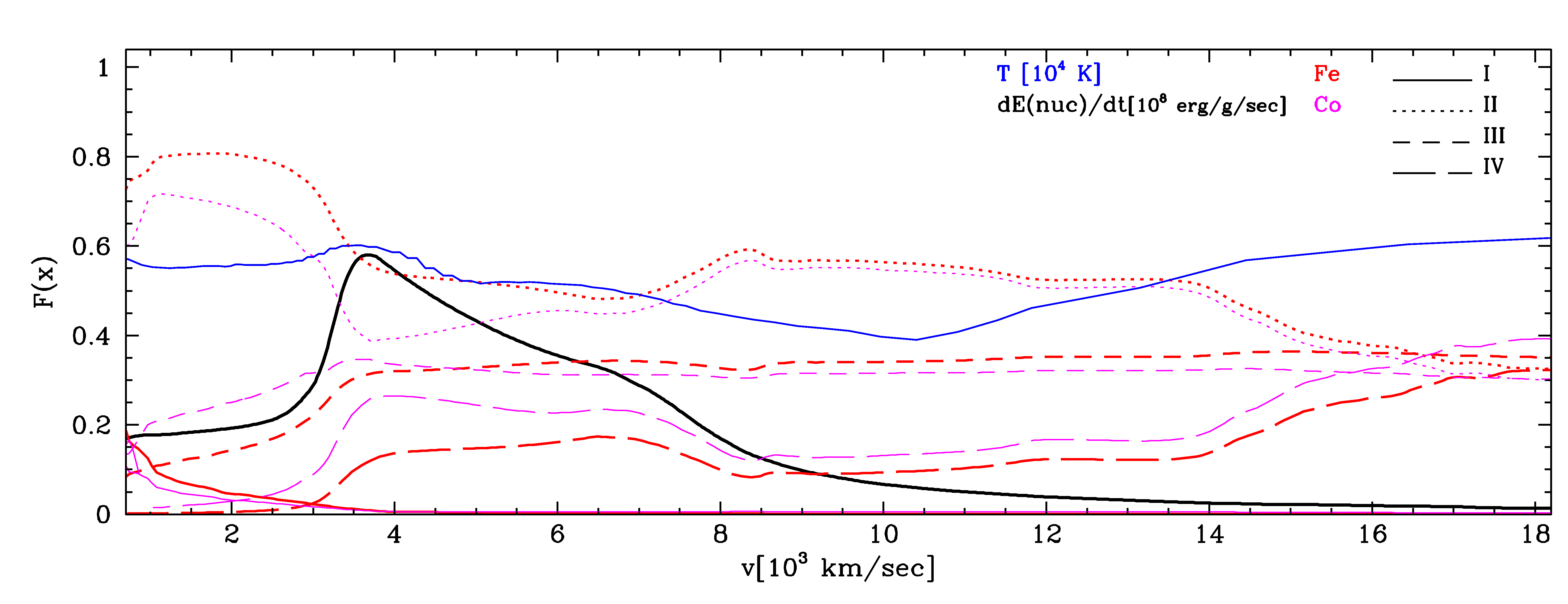
Figure 6: Angle averaged ionization levels I-IV of Fe and Co as representative of iron-group elements, specific energy input by $\gamma$-rays and non-thermal leptons, and temperature T as a function of expansion velocity of the underluminous model used for SN 2020qxp/ASASSN-20jq.

For illustration and as reference, the ionization level for Fe and Co is shown in Fig. 6 as representatives for iron-group elements. Intermediate mass elements, where present in the envelope, show a similar pattern but shifted to larger II/III/IV ratios. Because of the spherical density distribution, deviations from spherical symmetry remain rather small. In the line-forming region, the temperatures are 4000-5500 K with a peak coinciding with the maximum energy deposition. Unlike normal-bright SNe Ia of $M_{Ch}$ models with double ionized ions dominating at about day 210 (Wilk et al., 2018; Shingles et al., 2020), our subluminous SNe Ia shows the second ionization state dominating in the line-forming region. The overall lower dominant ionization stage is a result of the reduced ⁵⁶Ni mass, by a factor of $\approx 2...3$, and because the average ⁵⁶Ni is shifted to the inner, higher density regions (Fig. 2) boosting the recombination rate. Already by day 210, we see neutral iron group elements in the center. In our models, the rise of the ionization stage to III and IV at high velocities is caused by the low densities reducing the recombination rate, and the lower UV optical depth ’shutting off’ of the incomplete Rosseland cycle towards lower ions. Note that the ionization state shows only moderate variations in the line-forming region of the $1.644$ µm  feature lending additional stability to analysis of line profiles in this paper as discussed in Sect. 4.1.

Appendix B Optical Line Lists

In Tables B1-B4 we present line lists for relevant optical forbidden lines.

Table 3: Same as Table 2 but for synthetic spectra in the optical (Part 1).

S   $\lambda$[µm ]	Ion	S   $\lambda$[µm ]	Ion	S   $\lambda$[µm ]	Ion	S   $\lambda$[µm ]	Ion	S   $\lambda$[µm ]	Ion
0.3052	[Co II]	** 0.3077	[Ni II]	* 0.3083	[Co II]	0.3160	[Co II]	0.3174	[Co II]
* 0.3176	[Fe II]	* 0.3193	[Co II]	0.3202	[Co II]	0.3205	[Co II]	* 0.3216	[Fe II]
0.3219	[Co II]	0.3223	[Co II]	** 0.3224	[Ni II]	* 0.3225	[Fe II]	0.3241	[Fe III]
0.3244	[Co II]	* 0.3245	[Fe II]	** 0.3255	[Fe II]	0.3259	[Co II]	* 0.3276	[Fe II]
0.3278	[Fe II]	* 0.3279	[Fe II]	* 0.3290	[Fe II]	* 0.3291	[Fe II]	0.3296	[Co II]
0.3306	[Co II]	* 0.3306	[Co II]	0.3314	[Co II]	* 0.3319	[Fe II]	0.3326	[Co II]
0.3326	[Co II]	0.3364	[Co II]	* 0.3366	[Co II]	* 0.3377	[Co II]	** 0.3377	[Fe II]
0.3378	[Co II]	** 0.3379	[Ni II]	* 0.3382	[Fe II]	* 0.3382	[Co II]	0.3383	[Co II]
0.3383	[Co II]	** 0.3388	[Fe II]	* 0.3402	[Co II]	* 0.3404	[Fe II]	* 0.3421	[Co II]
0.3429	[Fe II]	0.3434	[Co II]	** 0.3440	[Ni II]	** 0.3442	[Fe II]	* 0.3451	[Fe II]
* 0.3453	[Fe II]	** 0.3456	[Fe II]	* 0.3485	[Fe II]	* 0.3491	[Fe II]	** 0.3503	[Fe II]
* 0.3505	[Fe II]	** 0.3505	[Fe II]	* 0.3507	[Fe II]	* 0.3529	[Fe II]	0.3529	[Co II]
0.3531	[Co II]	* 0.3534	[Fe II]	* 0.3537	[Fe II]	** 0.3540	[Fe II]	** 0.3540	[Fe II]
0.3557	[Co II]	0.3560	[Ni II]	** 0.3560	[Ni II]	0.3565	[Co II]	* 0.3577	[Fe II]
0.3580	[Ni II]	* 0.3581	[Fe II]	0.3583	[Co II]	* 0.3584	[Co II]	* 0.3589	[Fe II]
0.3599	[Co II]	* 0.3606	[Fe II]	* 0.3614	[Co II]	* 0.3621	[Co II]	* 0.3627	[Fe II]
0.3628	[Ni II]	** 0.3628	[Ni II]	* 0.3630	[Fe II]	0.3635	[Co II]	** 0.3638	[Co II]
0.3640	[Co II]	* 0.3641	[Co II]	* 0.3643	[Fe II]	* 0.3654	[Co II]	* 0.3666	[Fe II]
0.3679	[Co II]	** 0.3682	[Co II]	*** 0.3689	[Co II]	* 0.3710	[Co II]	* 0.3727	[O II]
0.3730	[O II]	0.3754	[Co II]	* 0.3754	[Co II]	** 0.3769	[Co II]	** 0.3771	[Co II]
0.3771	[Co II]	0.3799	[Co II]	** 0.3802	[Co II]	* 0.3845	[Ni II]	* 0.3848	[Co II]
0.3863	[Co II]	* 0.3977	[Co II]	* 0.3977	[Co II]	* 0.3981	[Co II]	* 0.3994	[Ni II]
0.4018	[Co II]	0.4026	[Ni II]	* 0.4034	[Ni II]	** 0.4070	[S II]	** 0.4078	[S II]
0.4083	[Fe II]	* 0.4085	[Fe II]	** 0.4104	[Co II]	* 0.4112	[Co II]	** 0.4116	[Fe II]
* 0.4121	[Co II]	0.4126	[Co II]	* 0.4133	[Co II]	* 0.4144	[Ni II]	* 0.4146	[Co II]
0.4148	[Ni II]	* 0.4150	[Co II]	* 0.4150	[Fe II]	*** 0.4154	[Co II]	* 0.4156	[Co II]
0.4159	[Fe II]	* 0.4171	[Co II]	* 0.4173	[Co II]	* 0.4178	[Co II]	** 0.4178	[Fe II]
0.4180	[Fe II]	0.4189	[Co II]	* 0.4199	[Fe II]	* 0.4202	[Ni II]	** 0.4212	[Fe II]
0.4216	[Co II]	* 0.4218	[Co II]	0.4225	[Co II]	* 0.4233	[Fe II]	* 0.4236	[Fe II]
** 0.4245	[Fe II]	*** 0.4246	[Fe II]	** 0.4246	[Co II]	* 0.4250	[Ni II]	* 0.4253	[Fe II]
* 0.4263	[Co II]	* 0.4267	[Co III]	* 0.4268	[Fe II]	* 0.4274	[Co II]	*** 0.4278	[Fe II]
0.4281	[Fe II]	* 0.4286	[Ni II]	*** 0.4289	[Fe II]	** 0.4289	[Co II]	* 0.4294	[Co II]
0.4295	[Ni II]	** 0.4307	[Fe II]	0.4312	[Ni II]	0.4313	[Co I]	0.4316	[Ni II]
0.4317	[Co II]	*** 0.4321	[Fe II]	** 0.4324	[Co II]	* 0.4327	[Ni II]	0.4327	[Co II]
0.4331	[Fe II]	0.4337	[Co III]	0.4345	[Co II]	*** 0.4348	[Fe II]	* 0.4353	[Co II]
0.4353	[Fe II]	*** 0.4354	[Fe II]	* 0.4357	[Fe II]	*** 0.4360	[Fe II]	*** 0.4361	[Fe II]
0.4362	[Co II]	* 0.4362	[Co II]	** 0.4364	[O III]	* 0.4365	[Co II]	*** 0.4374	[Fe II]
0.4377	[Co II]	* 0.4383	[Co II]	** 0.4384	[Fe II]	* 0.4384	[Fe II]	** 0.4389	[Co III]
0.4401	[Co III]	* 0.4404	[Fe II]	* 0.4411	[Co II]	* 0.4411	[Fe II]	* 0.4412	[Co II]
** 0.4415	[Fe II]	*** 0.4417	[Fe II]	* 0.4418	[Co II]	* 0.4426	[Co III]	** 0.4434	[Fe II]
0.4436	[Co II]	* 0.4438	[Co II]	* 0.4449	[Co II]	0.4449	[Co I]	0.4451	[Co II]
** 0.4453	[Fe II]	*** 0.4459	[Fe II]	* 0.4461	[Co II]	0.4463	[Ni II]	0.4467	[Ni II]
0.4468	[Co II]	* 0.4470	[Fe II]	** 0.4470	[Co III]	** 0.4472	[Fe II]	*** 0.4476	[Fe II]
0.4477	[Co I]	* 0.4480	[Fe II]	0.4487	[Ni II]	** 0.4487	[Ni II]	** 0.4490	[Fe II]
* 0.4494	[Fe II]	** 0.4501	[Co III]	0.4501	[Co III]	** 0.4509	[S I]	** 0.4511	[Fe II]
* 0.4516	[Fe II]	*** 0.4524	[Ni I]	0.4524	[Ni I]	0.4529	[Co II]	** 0.4530	[Fe II]
0.4530	[Co II]	* 0.4534	[Fe II]	** 0.4543	[Co II]	0.4549	[Co III]	0.4562	[Co I]

Table 4: Same as Table 2 but for synthetic spectra in the optical (Part 2).

S   $\lambda$[µm ]	Ion	S   $\lambda$[µm ]	Ion	S   $\lambda$[µm ]	Ion	S   $\lambda$[µm ]	Ion	S   $\lambda$[µm ]	Ion
0.4565	[Co II]	* 0.4567	[Ni I]	0.4569	[Co III]	0.4571	[Co III]	0.4575	[Ni II]
0.4578	[Fe II]	0.4583	[Co III]	** 0.4590	[S I]	* 0.4599	[Co I]	0.4608	[Fe III]
0.4613	[Co II]	0.4617	[Co I]	* 0.4623	[C I]	*** 0.4624	[Co II]	* 0.4628	[Co III]
0.4628	[Co III]	0.4629	[C I]	0.4629	[Ni II]	** 0.4629	[Ni II]	0.4631	[Co III]
** 0.4641	[Fe II]	** 0.4659	[Co II]	0.4660	[Fe III]	** 0.4666	[Fe II]	0.4668	[Fe III]
0.4685	[Co I]	0.4703	[Fe III]	** 0.4712	[Ni I]	0.4715	[Co III]	* 0.4719	[Co III]
** 0.4729	[Fe II]	0.4735	[Co II]	0.4735	[Fe III]	* 0.4738	[Co I]	* 0.4747	[Fe II]
* 0.4749	[Co II]	0.4756	[Fe III]	0.4771	[Fe III]	** 0.4773	[Fe II]	*** 0.4776	[Fe II]
0.4779	[Fe III]	0.4794	[Co II]	** 0.4800	[Fe II]	** 0.4804	[Co II]	* 0.4815	[Ni I]
** 0.4816	[Fe II]	0.4818	[Co II]	* 0.4837	[Co II]	0.4841	[Co II]	* 0.4854	[Fe II]
0.4875	[Co I]	*** 0.4876	[Fe II]	* 0.4880	[Co II]	*** 0.4891	[Fe II]	* 0.4899	[Co II]
* 0.4900	[Fe II]	*** 0.4907	[Fe II]	* 0.4910	[Co II]	* 0.4917	[Co III]	* 0.4920	[Co II]
0.4932	[Fe III]	0.4933	[O III]	** 0.4949	[Fe II]	** 0.4952	[Fe II]	*** 0.4960	[O III]
0.4960	[O III]	* 0.4972	[Co II]	0.4972	[Co I]	** 0.4975	[Fe II]	0.4989	[Co II]
0.4989	[Co III]	** 0.5007	[Fe II]	** 0.5008	[Fe II]	*** 0.5008	[O III]	0.5013	[Fe III]
0.5016	[Co II]	** 0.5022	[Fe II]	* 0.5029	[Ni I]	* 0.5029	[Fe II]	* 0.5031	[Co II]
0.5037	[Fe II]	0.5045	[Co II]	** 0.5045	[Fe II]	* 0.5050	[Fe II]	** 0.5062	[Fe II]
0.5066	[Ni II]	0.5070	[Co I]	** 0.5074	[Fe II]	* 0.5076	[Co I]	0.5076	[Co I]
0.5080	[Co I]	* 0.5081	[Co II]	0.5086	[Fe III]	** 0.5109	[Fe II]	*** 0.5113	[Fe II]
0.5115	[Co III]	0.5116	[Co II]	* 0.5116	[Co II]	* 0.5125	[Co II]	0.5134	[Ni II]
0.5137	[Co III]	* 0.5149	[Co II]	0.5149	[Co II]	*** 0.5160	[Fe II]	*** 0.5160	[Fe II]
* 0.5165	[Fe II]	* 0.5167	[Co III]	* 0.5174	[Fe II]	* 0.5177	[Co II]	** 0.5183	[Fe II]
* 0.5186	[Fe II]	* 0.5187	[Fe II]	0.5193	[Co II]	* 0.5193	[Co III]	* 0.5193	[Co III]
** 0.5221	[Fe II]	* 0.5229	[Co II]	0.5237	[Co I]	0.5237	[Co I]	0.5245	[Co I]
0.5246	[Co II]	0.5249	[Co III]	0.5249	[Co III]	0.5252	[Co I]	0.5253	[Co II]
0.5253	[Co II]	*** 0.5263	[Fe II]	0.5265	[Co I]	*** 0.5270	[Fe II]	** 0.5270	[Co II]
0.5271	[Ni II]	0.5272	[Fe III]	*** 0.5275	[Fe II]	* 0.5276	[Ni II]	* 0.5277	[Ni II]
0.5279	[Co II]	0.5283	[Ni II]	*** 0.5298	[Fe II]	0.5299	[Co II]	* 0.5300	[Co II]
0.5330	[Co II]	*** 0.5335	[Fe II]	* 0.5335	[Co III]	** 0.5349	[Fe II]	*** 0.5350	[Ni I]
0.5350	[Co I]	* 0.5359	[Co II]	0.5367	[Co II]	*** 0.5378	[Fe II]	0.5388	[Co II]
0.5400	[Co I]	0.5414	[Fe III]	0.5416	[Co II]	0.5416	[Co II]	0.5416	[Co I]
0.5433	[Ni II]	*** 0.5435	[Fe II]	* 0.5439	[Co II]	0.5448	[Co II]	0.5448	[Co II]
0.5456	[Co III]	0.5456	[Co III]	** 0.5472	[Co II]	** 0.5479	[Fe II]	0.5515	[Co I]
0.5528	[Co II]	** 0.5529	[Fe II]	* 0.5546	[Co II]	** 0.5548	[Co II]	** 0.5553	[Fe II]
* 0.5558	[Fe II]	** 0.5562	[Co II]	* 0.5572	[Co II]	* 0.5574	[Co II]	*** 0.5579	[O I]
* 0.5582	[Fe II]	* 0.5588	[Fe II]	* 0.5589	[Fe II]	* 0.5590	[Fe II]	* 0.5601	[Co II]
0.5615	[Fe II]	0.5620	[Co II]	0.5623	[Co I]	0.5625	[Co I]	* 0.5629	[Co III]
0.5629	[Fe II]	** 0.5641	[Fe I]	* 0.5651	[Fe II]	* 0.5652	[Fe II]	* 0.5659	[Co II]
0.5665	[Co II]	0.5670	[Co I]	* 0.5670	[Mn I]	** 0.5675	[Fe II]	* 0.5676	[Co II]
0.5680	[Co II]	** 0.5683	[Co II]	0.5690	[Co I]	* 0.5692	[Mn I]	** 0.5698	[Fe I]
0.5705	[Ni II]	** 0.5711	[Fe I]	0.5713	[Ni II]	* 0.5720	[Fe II]	* 0.5726	[Co II]
0.5727	[Fe II]	** 0.5730	[Mn I]	** 0.5731	[Co II]	* 0.5746	[Co II]	** 0.5749	[Fe II]
0.5758	[Co I]	* 0.5758	[Fe II]	* 0.5769	[Fe II]	* 0.5777	[Fe I]	** 0.5786	[Mn I]
0.5801	[Fe II]	0.5803	[Co I]	** 0.5806	[Fe I]	* 0.5816	[Co II]	** 0.5836	[Fe I]
* 0.5837	[Fe II]	0.5841	[Co III]	* 0.5846	[Fe II]	* 0.5849	[Fe II]	** 0.5864	[Mn I]
0.5869	[Fe I]	** 0.5872	[Fe II]	** 0.5874	[Fe I]	0.5888	[Co I]	*** 0.5890	[Co III]
0.5892	[Co II]	0.5894	[Co I]	* 0.5903	[Fe II]	** 0.5908	[Co III]	* 0.5915	[Fe II]

Table 5: Same as Table 2 but for synthetic spectra in the optical (Part 3). Note that the [CaII] doublet at $0.7293/0.7326\mu$m is dominating beyond scale. Without Ca, there would still be significant features comparable to those at shorter wavelengths as is obvious from the red ’component’ of model 03 (see inset of Fig. 4).

S   $\lambda$[µm ]	Ion	S   $\lambda$[µm ]	Ion	S   $\lambda$[µm ]	Ion	S   $\lambda$[µm ]	Ion	S   $\lambda$[µm ]	Ion
0.5925	[Co II]	** 0.5936	[Fe I]	** 0.5939	[Fe I]	0.5943	[Co III]	0.5951	[Co II]
0.5956	[Co II]	* 0.5960	[Co I]	* 0.5961	[Co II]	** 0.5971	[Fe I]	* 0.5984	[Fe II]
0.5989	[Co II]	0.5989	[Co II]	* 0.6002	[Fe I]	* 0.6009	[Ni II]	0.6016	[Co II]
0.6020	[Co II]	0.6022	[Co II]	0.6031	[Co I]	** 0.6046	[Fe II]	0.6051	[Co I]
0.6058	[Co II]	0.6059	[Co II]	* 0.6072	[Co I]	0.6075	[Co II]	* 0.6091	[Co I]
0.6097	[Fe II]	0.6113	[Co II]	0.6113	[Co I]	** 0.6129	[Co III]	* 0.6149	[Co II]
0.6154	[Co II]	* 0.6187	[Co II]	0.6188	[Co II]	* 0.6190	[Fe II]	** 0.6190	[Fe II]
* 0.6197	[Co III]	0.6210	[Co III]	* 0.6247	[Co II]	0.6253	[Co II]	0.6258	[Co II]
0.6263	[Fe II]	0.6265	[Co I]	* 0.6265	[Co I]	* 0.6276	[Co II]	* 0.6282	[Fe II]
0.6289	[Co II]	0.6295	[Co II]	*** 0.6302	[O I]	* 0.6302	[O I]	0.6303	[Co II]
0.6316	[Co II]	* 0.6318	[Co I]	0.6343	[Co I]	0.6352	[Co I]	0.6352	[Co I]
0.6355	[Fe II]	0.6356	[Co II]	0.6356	[Co II]	0.6365	[Co I]	*** 0.6366	[O I]
0.6366	[O I]	* 0.6367	[Ni II]	* 0.6388	[Co I]	* 0.6389	[Co I]	0.6393	[O I]
0.6398	[Fe II]	0.6400	[Co II]	** 0.6406	[Ni I]	* 0.6406	[Fe II]	0.6426	[Co II]
* 0.6439	[Ni I]	* 0.6443	[Ni II]	* 0.6469	[Ni II]	0.6471	[Co II]	* 0.6476	[Fe II]
0.6476	[Fe II]	* 0.6484	[Fe II]	* 0.6487	[Fe II]	** 0.6491	[Ni I]	0.6506	[Co I]
0.6506	[Co I]	* 0.6513	[Fe II]	** 0.6521	[Co II]	* 0.6529	[Si I]	* 0.6547	[Fe II]
0.6568	[Fe II]	** 0.6578	[Co III]	* 0.6586	[Co I]	* 0.6586	[Fe II]	0.6591	[Si I]
* 0.6606	[Ni I]	* 0.6634	[Co II]	0.6639	[Co I]	* 0.6639	[Co I]	0.6652	[Co I]
0.6669	[Ni II]	* 0.6674	[Fe II]	0.6680	[Co I]	0.6680	[Co I]	* 0.6685	[Co I]
0.6691	[Fe II]	0.6702	[Ni II]	* 0.6702	[Fe II]	0.6707	[Co II]	* 0.6710	[Mn II]
0.6718	[S II]	** 0.6732	[Fe II]	* 0.6732	[Ni I]	* 0.6733	[S II]	* 0.6733	[Co II]
0.6747	[Co II]	* 0.6748	[Fe II]	* 0.6749	[Fe II]	* 0.6762	[Co I]	0.6765	[Mn II]
0.6789	[Ni I]	0.6792	[Co I]	* 0.6793	[Ni II]	* 0.6796	[Ni II]	0.6799	[Co II]
0.6806	[Co I]	** 0.6811	[Fe II]	* 0.6815	[Ni II]	0.6821	[Co I]	0.6830	[Co II]
0.6831	[Fe II]	* 0.6850	[Ni II]	* 0.6852	[Mn II]	* 0.6851	[Co III]	** 0.6855	[Co III]
* 0.6874	[Fe II]	** 0.6876	[Fe II]	0.6878	[Co II]	* 0.6888	[Co II]	** 0.6898	[Fe II]
0.6907	[Co I]	* 0.6913	[Ni II]	0.6925	[Fe II]	* 0.6926	[Co II]	** 0.6934	[Co II]
0.6936	[Fe II]	** 0.6944	[Ni I]	** 0.6947	[Fe II]	* 0.6951	[Co I]	* 0.6958	[Ni II]
0.6958	[Ni II]	* 0.6963	[Co III]	* 0.6964	[Co III]	** 0.6968	[Fe II]	* 0.6974	[Co I]
0.6981	[Co II]	** 0.7004	[Ni I]	* 0.7012	[Co II]	* 0.7013	[Fe II]	0.7014	[Co III]
0.7019	[Co I]	0.7030	[Co II]	* 0.7031	[Co II]	0.7037	[Co II]	* 0.7050	[Fe II]
0.7052	[Co II]	* 0.7053	[Co II]	* 0.7056	[Ni II]	* 0.7080	[Ni II]	0.7100	[Co I]
0.7102	[Co II]	0.7105	[Ni II]	** 0.7132	[Ni I]	* 0.7133	[Fe II]	* 0.7135	[Co I]
0.7142	[Co II]	0.7145	[Co II]	0.7147	[Co II]	* 0.7155	[Co III]	*** 0.7157	[Fe II]
0.7161	[Co I]	0.7162	[Co III]	* 0.7171	[Co III]	0.7173	[Co II]	*** 0.7174	[Fe II]
* 0.7196	[Ni I]	0.7204	[Co III]	* 0.7221	[Ni I]	* 0.7249	[Co I]	* 0.7258	[Ni II]
0.7258	[Co II]	0.7258	[Co I]	* 0.7272	[Co III]	* 0.7277	[Co II]	**** 0.7293	[Ca II]
0.7300	[Co I]	0.7300	[Co I]	* 0.7310	[Ni II]	* 0.7321	[O II]	** 0.7322	[O II]
*** 0.7326	[Ca II]	* 0.7332	[O II]	* 0.7332	[O II]	* 0.7332	[Fe II]	* 0.7333	[O II]
0.7333	[O II]	0.7360	[Co III]	0.7365	[Co II]	* 0.7372	[Co II]	* 0.7373	[Fe II]
0.7373	[Co II]	* 0.7374	[Co III]	* 0.7375	[Co II]	* 0.7380	[Ni II]	*** 0.7390	[Fe II]
0.7394	[Co II]	* 0.7396	[Ni I]	* 0.7398	[Ni I]	* 0.7410	[Co II]	0.7414	[Ni II]
0.7424	[Co II]	0.7430	[Co I]	* 0.7434	[Fe II]	0.7447	[Co II]	*** 0.7455	[Fe II]

Table 6: Same as Table 2 but for synthetic spectra in the optical (Part 4).

S   $\lambda$[µm ]	Ion	S   $\lambda$[µm ]	Ion	S   $\lambda$[µm ]	Ion	S   $\lambda$[µm ]	Ion	S   $\lambda$[µm ]	Ion
* 0.7466	[Ni I]	* 0.7469	[Co II]	0.7477	[Co I]	* 0.7482	[Co II]	* 0.7499	[Co III]
* 0.7509	[Ni I]	0.7511	[Co I]	* 0.7521	[Co I]	0.7522	[Co II]	0.7526	[Co II]
* 0.7541	[Co II]	* 0.7556	[Co II]	* 0.7564	[Co I]	* 0.7570	[Co II]	0.7584	[Co II]
0.7614	[Co II]	* 0.7615	[Ni II]	* 0.7615	[Fe II]	0.7639	[Co I]	0.7639	[Co I]
* 0.7640	[Fe II]	* 0.7640	[Co II]	* 0.7645	[Co II]	* 0.7658	[Co I]	* 0.7667	[Fe II]
* 0.7689	[Fe II]	0.7697	[Ni II]	0.7701	[Co I]	* 0.7704	[Co I]	0.7706	[Co II]
0.7722	[Fe II]	* 0.7725	[Co II]	*** 0.7727	[S I]	0.7731	[Co II]	* 0.7735	[Fe II]
0.7737	[Fe II]	0.7757	[Co II]	** 0.7767	[Fe II]	* 0.7796	[Co II]	0.7822	[Co III]
0.7832	[Co II]	* 0.7837	[Co II]	* 0.7840	[Co I]	* 0.7876	[Fe II]	** 0.7910	[Ni I]
0.7914	[Co I]	* 0.7918	[Co I]	* 0.7926	[Co II]	0.7932	[Ni I]	* 0.7936	[Co II]
0.7936	[Co II]	* 0.7943	[Co I]	0.7972	[Co I]	* 0.7977	[Fe II]	0.7992	[Ni I]
0.8030	[Co II]	* 0.8036	[Ni II]	0.8036	[Ni II]	* 0.8047	[Fe II]	* 0.8049	[Co II]
0.8072	[Co I]	* 0.8080	[Fe II]	* 0.8112	[Co I]	* 0.8114	[Ni I]	** 0.8123	[Co II]
0.8179	[Co I]	0.8180	[Co II]	* 0.8197	[Ni I]	* 0.8199	[Co II]	* 0.8201	[Fe II]
0.8204	[Ni I]	* 0.8262	[Fe II]	0.8273	[Co I]	* 0.8303	[Ni II]	0.8306	[Co I]
* 0.8308	[Fe II]	* 0.8336	[Co II]	0.8343	[Co I]	** 0.8389	[Fe II]	* 0.8413	[Co II]
0.8414	[Fe II]	* 0.8466	[Co II]	* 0.8469	[Ni I]	* 0.8469	[Co II]	* 0.8482	[Fe II]
0.8489	[Co I]	* 0.8492	[Fe II]	0.8500	[Co II]	* 0.8543	[Co II]	0.8545	[Co I]
0.8546	[Co I]	** 0.8574	[Co II]	* 0.8577	[Fe II]	* 0.8578	[Fe II]	* 0.8583	[Co II]
0.8597	[Co I]	* 0.8602	[Co II]	** 0.8603	[Fe II]	*** 0.8619	[Fe II]	* 0.8626	[Co II]
0.8691	[Co I]	0.8694	[Co II]	* 0.8706	[Ni II]	* 0.8709	[Co II]	* 0.8711	[Fe II]
* 0.8718	[Fe II]	*** 0.8730	[C I]	* 0.8737	[Fe II]	* 0.8741	[Fe II]	0.8776	[Co I]
0.8827	[Fe II]	** 0.8835	[Ni I]	** 0.8846	[Ni I]	* 0.8855	[Co II]	* 0.8864	[Fe II]
0.8888	[Fe II]	** 0.8894	[Fe II]	0.8899	[Ni II]	0.8899	[Co II]	* 0.8934	[Fe II]
0.8968	[Co II]	* 0.8993	[Co I]	* 0.9015	[Co II]	* 0.9022	[Co I]	** 0.9036	[Fe II]
* 0.9054	[Fe II]	* 0.9057	[Co I]	* 0.9085	[Co II]	* 0.9086	[Fe II]	* 0.9135	[Co I]
0.9136	[Fe II]	0.9149	[Co II]	* 0.9205	[Fe II]	* 0.9205	[Co II]	** 0.9229	[Fe II]
* 0.9234	[Fe II]	* 0.9247	[Co II]	** 0.9270	[Fe II]	** 0.9338	[Co II]	*** 0.9345	[Co II]
0.9347	[Co I]	* 0.9354	[Fe II]	* 0.9372	[Co II]	0.9377	[Ni II]	* 0.9384	[Fe II]
0.9387	[Fe II]	* 0.9414	[Fe I]	* 0.9439	[Fe II]	0.9447	[Fe III]	* 0.9468	[Fe II]
0.9472	[Fe II]	** 0.9474	[Fe II]	* 0.9493	[Fe II]	* 0.9517	[Fe II]	0.9529	[Co I]
0.9541	[Co II]	* 0.9555	[Fe II]	* 0.9593	[Fe II]	** 0.9642	[Co II]	* 0.9662	[Fe I]
0.9672	[Fe II]	* 0.9685	[Fe II]	* 0.9696	[Co I]	0.9704	[Fe III]	* 0.9714	[Fe II]
0.9760	[Ni II]	* 0.9805	[Fe I]	** 0.9827	[C I]	* 0.9829	[Fe I]	** 0.9853	[C I]

References

- Ann et al. (2015) Ann, H. B., Seo, M., & Ha, D. K. 2015, ApJS, 217, 27, doi: 10.1088/0067-0049/217/2/27
- Ashall et al. (2018) Ashall, C., Mazzali, P. A., Stritzinger, M. D., et al. 2018, MNRAS, 477, 153, doi: 10.1093/mnras/sty632
- Ashall et al. (2019) Ashall, C., Hsiao, E. Y., Hoeflich, P., et al. 2019, ApJ, 875, L14, doi: 10.3847/2041-8213/ab1654
- Ashall et al. (2021) Ashall, C., Baron, E., Hoeflich, P. A., et al. 2021, MIR Spectroscopy of Type Ia Supernovae: The Key to Unlocking their Explosions and Element Production, JWST Proposal. Cycle 1
- Axelrod (1980a) Axelrod, T. S. 1980a, PhD thesis, California Univ., Santa Cruz.
- Axelrod (1980b) —. 1980b, PhD thesis, California Univ., Santa Cruz.
- Badenes et al. (2006) Badenes, C., Borkowski, K. J., Hughes, J. P., Hwang, U., & Bravo, E. 2006, ApJ, 645, 1373, doi: 10.1086/504399
- Badenes et al. (2003) Badenes, C., Bravo, E., Borkowski, K. J., & Domínguez, I. 2003, ApJ, 593, 358, doi: 10.1086/376448
- Benetti et al. (2005) Benetti, S., Cappellaro, E., Mazzali, P. A., et al. 2005, ApJ, 623, 1011, doi: 10.1086/428608
- Benz et al. (1990) Benz, W., Cameron, A. G. W., Press, W. H., & Bowers, R. L. 1990, ApJ, 348, 647, doi: 10.1086/168273
- Berger et al. (1998) Berger, M. B., Hubbell, J. H., Seltzer, S., Coursey, J., & Zucker, D. 1998, NBSIR, 87-3597, ”http://physics.nist.gov/PhysRefData/Xcom/Text/XCOM.html”
- Bessell (1990) Bessell, M. S. 1990, PASP, 102, 1181, doi: 10.1086/132749
- Blondin et al. (2015) Blondin, S., Dessart, L., & Hillier, D. J. 2015, MNRAS, 448, 2766, doi: 10.1093/mnras/stv188
- Blondin et al. (2018) —. 2018, MNRAS, 474, 3931, doi: 10.1093/mnras/stx3058
- Blondin et al. (2017) Blondin, S., Dessart, L., Hillier, D. J., & Khokhlov, A. M. 2017, MNRAS, 470, 157, doi: 10.1093/mnras/stw2492
- Botyánszki & Kasen (2017a) Botyánszki, J., & Kasen, D. 2017a, ApJ, 845, 176, doi: 10.3847/1538-4357/aa81d8
- Botyánszki & Kasen (2017b) —. 2017b, ApJ, 845, 176, doi: 10.3847/1538-4357/aa81d8
- Brachwitz et al. (2000) Brachwitz, F., Dean, D. J., Hix, W. R., et al. 2000, ApJ, 536, 934, doi: 10.1086/308968
- Branch et al. (2005) Branch, D., Baron, E., Hall, N., Melakayil, M., & Parrent, J. 2005, PASP, 117, 545, doi: 10.1086/430135
- Branch et al. (2009) Branch, D., Chau Dang, L., & Baron, E. 2009, PASP, 121, 238, doi: 10.1086/597788
- Brooker et al. (2021) Brooker, E., Plewa, T., & Fenn, D. 2021, MNRAS, 501, L23, doi: 10.1093/mnrasl/slaa141
- Bulla et al. (2016) Bulla, M., Sim, S. A., Kromer, M., et al. 2016, MNRAS, 462, 1039, doi: 10.1093/mnras/stw1733
- Burns et al. (2011) Burns, C. R., Stritzinger, M., Phillips, M. M., et al. 2011, AJ, 141, 19, doi: 10.1088/0004-6256/141/1/19
- Burns et al. (2018) Burns, C. R., Parent, E., Phillips, M. M., et al. 2018, ApJ, 869, 56, doi: 10.3847/1538-4357/aae51c
- Burns et al. (2020) Burns, C. R., Ashall, C., Contreras, C., et al. 2020, ApJ, 895, 118, doi: 10.3847/1538-4357/ab8e3e
- Cappellaro et al. (1997) Cappellaro, E., Mazzali, P. A., Benetti, S., et al. 1997, A&A, 328, 203. https://arxiv.org/abs/astro-ph/9707016
- Cikota et al. (2019a) Cikota, A., Patat, F., Wang, L., et al. 2019a, MNRAS, 490, 578, doi: 10.1093/mnras/stz2322
- Cikota et al. (2019b) —. 2019b, MNRAS, 490, 578, doi: 10.1093/mnras/stz2322
- Colella & Woodward (1984) Colella, P., & Woodward, P. R. 1984, Journal of Computational Physics, 54, 174, doi: 10.1016/0021-9991(84)90143-8
- Cushing et al. (2004) Cushing, M. C., Vacca, W. D., & Rayner, J. T. 2004, PASP, 116, 362, doi: 10.1086/382907
- Cyburt et al. (2010) Cyburt, R. H., Amthor, A. M., Ferguson, R., et al. 2010, ApJS, 189, 240, doi: 10.1088/0067-0049/189/1/240
- Di Stefano et al. (2011) Di Stefano, R., Voss, R., & Claeys, J. S. W. 2011, in AAS/High Energy Astrophysics Division, Vol. 12, AAS/High Energy Astrophysics Division, 33.04
- Diamond et al. (2015) Diamond, T. R., Hoeflich, P., & Gerardy, C. L. 2015, ApJ, 806, 107, doi: 10.1088/0004-637X/806/1/107
- Diamond et al. (2018) Diamond, T. R., Hoeflich, P., Hsiao, E. Y., et al. 2018, ApJ, 861, 119, doi: 10.3847/1538-4357/aac434
- Domínguez & Höflich (2000) Domínguez, I., & Höflich, P. 2000, ApJ, 528, 854, doi: 10.1086/308223
- Dong et al. (2015) Dong, S., Katz, B., Kushnir, D., & Prieto, J. L. 2015, MNRAS, 454, L61, doi: 10.1093/mnrasl/slv129
- Fesen et al. (2015) Fesen, R. A., Höflich, P. A., & Hamilton, A. J. S. 2015, ApJ, 804, 140, doi: 10.1088/0004-637X/804/2/140
- Fesen et al. (2007) Fesen, R. A., Höflich, P. A., Hamilton, A. J. S., et al. 2007, ApJ, 658, 396, doi: 10.1086/510998
- Flörs et al. (2020) Flörs, A., Spyromilio, J., Taubenberger, S., et al. 2020, MNRAS, 491, 2902, doi: 10.1093/mnras/stz3013
- Folatelli et al. (2013) Folatelli, G., Morrell, N., Phillips, M. M., et al. 2013, ApJ, 773, 53, doi: 10.1088/0004-637X/773/1/53
- Fransson & Jerkstrand (2015a) Fransson, C., & Jerkstrand, A. 2015a, ApJ, 814, L2, doi: 10.1088/2041-8205/814/1/L2
- Fransson & Jerkstrand (2015b) —. 2015b, ApJ, 814, L2, doi: 10.1088/2041-8205/814/1/L2
- Fransson & Sonneborn (1994) Fransson, C., & Sonneborn, G. 1994, Supernovae, ed. W. Wamsteker, M. S. Longair, & Y. Kondo, Vol. 187, 249, doi: 10.1007/978-94-011-0794-5_26
- Friesen et al. (2017) Friesen, B., Baron, E., Parrent, J. T., et al. 2017, MNRAS, 467, 2392, doi: 10.1093/mnras/stx241
- Fryxell (2001) Fryxell, B. 2001, in American Institute of Physics Conference Series, Vol. 583, American Institute of Physics Conference Series, 310–312, doi: 10.1063/1.1405335
- Fryxell et al. (1991) Fryxell, B., Mueller, E., & Arnett, D. 1991, ApJ, 367, 619, doi: 10.1086/169657
- Galbany et al. (2019a) Galbany, L., Ashall, C., Höflich, P., et al. 2019a, A&A, 630, A76, doi: 10.1051/0004-6361/201935537
- Galbany et al. (2019b) —. 2019b, A&A, 630, A76, doi: 10.1051/0004-6361/201935537
- Gall et al. (2018) Gall, C., Stritzinger, M. D., Ashall, C., et al. 2018, A&A, 611, A58, doi: 10.1051/0004-6361/201730886
- Gamezo et al. (2005) Gamezo, V. N., Khokhlov, A. M., & Oran, E. S. 2005, ApJ, 623, 337, doi: 10.1086/428767
- Gamezo et al. (2003) Gamezo, V. N., Khokhlov, A. M., Oran, E. S., Chtchelkanova, A. Y., & Rosenberg, R. O. 2003, Science, 299, 77, doi: 10.1126/science.299.5603.77
- García-Berro & Lorén-Aguilar (2017) García-Berro, E., & Lorén-Aguilar, P. 2017, Dynamical Mergers, ed. A. W. Alsabti & P. Murdin, 1237, doi: 10.1007/978-3-319-21846-5_60
- Gerardy et al. (2004) Gerardy, C. L., Höflich, P., Fesen, R. A., et al. 2004, ApJ, 607, 391, doi: 10.1086/383488
- Glasner et al. (2018) Glasner, S. A., Livne, E., Steinberg, E., Yalinewich, A., & Truran, J. W. 2018, MNRAS, 476, 2238, doi: 10.1093/mnras/sty421
- Graham et al. (2017) Graham, M. L., Kumar, S., Hosseinzadeh, G., et al. 2017, MNRAS, 472, 3437, doi: 10.1093/mnras/stx2224
- Graur et al. (2017) Graur, O., Bianco, F. B., Modjaz, M., et al. 2017, ApJ, 837, 121, doi: 10.3847/1538-4357/aa5eb7
- Gronow et al. (2021) Gronow, S., Collins, C. E., Sim, S. A., & Röpke, F. K. 2021, A&A, 649, A155, doi: 10.1051/0004-6361/202039954
- Han & Podsiadlowski (2006) Han, Z., & Podsiadlowski, P. 2006, MNRAS, 368, 1095, doi: 10.1111/j.1365-2966.2006.10185.x
- Hillier (1990) Hillier, D. J. 1990, A&A, 231, 116
- Hoeflich (1990) Hoeflich, P. 1990, A&A, 229, 191
- Hoeflich (2006) —. 2006, Nuclear Physics A, 777, 579, doi: 10.1016/j.nuclphysa.2004.12.038
- Hoeflich (2017) Hoeflich, P. 2017, in Handbook of Supernovae, ed. A. W. Alsabti & P. Murdin (Berlin: Springer), 1151, doi: 10.1007/978-3-319-21846-5_56
- Hoeflich & Khokhlov (1996) Hoeflich, P., & Khokhlov, A. 1996, ApJ, 457, 500, doi: 10.1086/176748
- Hoeflich et al. (2017a) Hoeflich, P., Hsiao, E. Y., Ashall, C., et al. 2017a, ApJ, 846, 58, doi: 10.3847/1538-4357/aa84b2
- Hoeflich et al. (2017b) —. 2017b, ApJ, 846, 58, doi: 10.3847/1538-4357/aa84b2
- Hoeflich et al. (2019) Hoeflich, P., Ashall, C., Fisher, A., et al. 2019, in Nuclei in the Cosmos XV, Vol. 219, 187–194, doi: 10.1007/978-3-030-13876-9_31
- Höflich (1995a) Höflich, P. 1995a, ApJ, 443, 89, doi: 10.1086/175505
- Höflich (1995b) —. 1995b, ApJ, 440, 821, doi: 10.1086/175317
- Höflich (2002) —. 2002, NAR, 46, 475, doi: 10.1016/S1387-6473(02)00186-0
- Höflich (2003) Höflich, P. 2003, in Astronomical Society of the Pacific Conference Series, Vol. 288, Stellar Atmosphere Modeling, ed. I. Hubeny, D. Mihalas, & K. Werner, 185
- Höflich (2009) Höflich, P. 2009, in American Institute of Physics Conference Series, Vol. 1171, American Institute of Physics Conference Series, ed. I. Hubeny, J. M. Stone, K. MacGregor, & K. Werner, 161–172, doi: 10.1063/1.3250057
- Höflich et al. (2002) Höflich, P., Gerardy, C. L., Fesen, R. A., & Sakai, S. 2002, ApJ, 568, 791, doi: 10.1086/339063
- Höflich et al. (2006) Höflich, P., Gerardy, C. L., Marion, H., & Quimby, R. 2006, New Astronomy Reviews, 50, 470, doi: 10.1016/j.newar.2006.06.074
- Höflich et al. (2004) Höflich, P., Gerardy, C. L., Nomoto, K., et al. 2004, ApJ, 617, 1258, doi: 10.1086/425571
- Höflich et al. (1992) Höflich, P., Khokhlov, A., & Müller, E. 1992, A&A, 259, 549
- Howell et al. (2001) Howell, D. A., Höflich, P., Wang, L., & Wheeler, J. C. 2001, ApJ, 556, 302, doi: 10.1086/321584
- Hoyle & Fowler (1960) Hoyle, F., & Fowler, W. A. 1960, ApJ, 132, 565, doi: 10.1086/146963
- Hristov et al. (2018) Hristov, B., Collins, D. C., Hoeflich, P., Weatherford, C. A., & Diamond, T. R. 2018, ApJ, 858, 13, doi: 10.3847/1538-4357/aab7f2
- Hristov et al. (2021) Hristov, B., Hoeflich, P., & Collins, D. C. 2021, arXiv e-prints, submitted to ApJ, arXiv:2106.14589. https://arxiv.org/abs/2106.14589
- Iben & Tutukov (1984) Iben, I., J., & Tutukov, A. V. 1984, ApJS, 54, 335, doi: 10.1086/190932
- Isern et al. (2011) Isern, J., Hernanz, M., & José, J. 2011, in Lecture Notes in Physics, ed. R. Diehl, D. H. Hartmann, & N. Prantzos, Vol. 812 (Berlin: Springer-Verlag), 233–308
- Jacobson-Galán et al. (2020) Jacobson-Galán, W. V., Polin, A., Foley, R. J., et al. 2020, ApJ, 896, 165, doi: 10.3847/1538-4357/ab94b8
- Jerkstrand et al. (2011) Jerkstrand, A., Fransson, C., & Kozma, C. 2011, A&A, 530, A45, doi: 10.1051/0004-6361/201015937
- Kaastra & Mewe (1993) Kaastra, J. S., & Mewe, R. 1993, A&AS, 97, 443
- Kasen et al. (2006) Kasen, D., Thomas, R. C., & Nugent, P. 2006, ApJ, 651, 366, doi: 10.1086/506190
- Kerzendorf & Sim (2014) Kerzendorf, W. E., & Sim, S. A. 2014, MNRAS, 440, 387, doi: 10.1093/mnras/stu055
- Khokhlov & Höflich (2001) Khokhlov, A., & Höflich, P. 2001, in American Institute of Physics Conference Series, Vol. 556, Explosive Phenomena in Astrophysical Compact Objects, ed. H.-Y. Chang, C.-H. Lee, M. Rho, & I. Yi, 301–312, doi: 10.1063/1.1368287
- Khokhlov (1989) Khokhlov, A. M. 1989, MNRAS, 239, 785, doi: 10.1093/mnras/239.3.785
- Khokhlov (1995) —. 1995, ApJ, 449, 695, doi: 10.1086/176091
- Kochanek et al. (2017) Kochanek, C. S., Shappee, B. J., Stanek, K. Z., et al. 2017, PASP, 129, 104502, doi: 10.1088/1538-3873/aa80d9
- Kourkchi et al. (2020) Kourkchi, E., Tully, R. B., Eftekharzadeh, S., et al. 2020, ApJ, 902, 145, doi: 10.3847/1538-4357/abb66b
- Kozma & Fransson (1992) Kozma, C., & Fransson, C. 1992, ApJ, 390, 602, doi: 10.1086/171311
- Kromer et al. (2010) Kromer, M., Sim, S. A., Fink, M., et al. 2010, ApJ, 719, 1067, doi: 10.1088/0004-637X/719/2/1067
- Kushnir et al. (2013) Kushnir, D., Katz, B., Dong, S., Livne, E., & Fernández, R. 2013, ApJ, 778, L37, doi: 10.1088/2041-8205/778/2/L37
- Langanke et al. (2004) Langanke, K., Martínez-Pinedo, G., von Neumann-Cosel, P., & Richter, A. 2004, Phys. Rev. Lett., 93, 202501, doi: 10.1103/PhysRevLett.93.202501
- Leonard et al. (2005) Leonard, D. C., Li, W., Filippenko, A. V., Foley, R. J., & Chornock, R. 2005, ApJ, 632, 450, doi: 10.1086/432866
- Li et al. (2001) Li, W., Filippenko, A. V., Gates, E., et al. 2001, PASP, 113, 1178, doi: 10.1086/323355
- Lidov (1962) Lidov, M. L. 1962, Planet. Space Sci., 9, 719, doi: 10.1016/0032-0633(62)90129-0
- Liu et al. (1998) Liu, W., Jeffery, D. J., & Schultz, D. R. 1998, ApJ, 494, 812, doi: 10.1086/305249
- Livne (1990) Livne, E. 1990, ApJ, 354, L53, doi: 10.1086/185721
- Livne (1999) —. 1999, ApJ, 527, L97, doi: 10.1086/312405
- Livne & Arnett (1995) Livne, E., & Arnett, D. 1995, ApJ, 452, 62, doi: 10.1086/176279
- Livne et al. (2005) Livne, E., Asida, S. M., & Hoeflich, P. 2005, ApJ, 632, 443
- Lorén-Aguilar et al. (2009) Lorén-Aguilar, P., Isern, J., & García-Berro, E. 2009, A&A, 500, 1193, doi: 10.1051/0004-6361/200811060
- Maeda et al. (2010) Maeda, K., Benetti, S., Stritzinger, M., et al. 2010, Nature, 466, 82, doi: 10.1038/nature09122
- Maeda et al. (2011) Maeda, K., Leloudas, G., Taubenberger, S., et al. 2011, MNRAS, 413, 3075, doi: 10.1111/j.1365-2966.2011.18381.x
- Maguire et al. (2018) Maguire, K., Sim, S. A., Shingles, L., et al. 2018, MNRAS, 477, 3567, doi: 10.1093/mnras/sty820
- Maund et al. (2013) Maund, J. R., Spyromilio, J., Hoflich, P. A., et al. 2013, MNRAS, 433, L20, doi: 10.1093/mnrasl/slt050
- Mazzali et al. (2018) Mazzali, P. A., Ashall, C., Pian, E., et al. 2018, MNRAS, 476, 2905, doi: 10.1093/mnras/sty434
- Mazzali et al. (2014) Mazzali, P. A., Sullivan, M., Hachinger, S., et al. 2014, MNRAS, 439, 1959, doi: 10.1093/mnras/stu077
- Motohara et al. (2006) Motohara, K., Maeda, K., Gerardy, C. L., et al. 2006, ApJ, 652, L101, doi: 10.1086/509919
- Niemeyer et al. (1996) Niemeyer, J. C., Hillebrandt, W., & Woosley, S. E. 1996, ApJ, 471, 903, doi: 10.1086/178017
- Nomoto (1982) Nomoto, K. 1982, ApJ, 257, 780, doi: 10.1086/160031
- Nomoto et al. (1984) Nomoto, K., Thielemann, F.-K., & Yokoi, K. 1984, ApJ, 286, 644, doi: 10.1086/162639
- Ohshiro et al. (2021) Ohshiro, Y., Yamaguchi, H., Leung, S.-C., et al. 2021, arXiv e-prints, arXiv:2105.04101. https://arxiv.org/abs/2105.04101
- Pakmor (2017) Pakmor, R. 2017, Violent Mergers, ed. A. W. Alsabti & P. Murdin, 1257, doi: 10.1007/978-3-319-21846-5_61
- Pakmor et al. (2012) Pakmor, R., Edelmann, P., Röpke, F. K., & Hillebrandt, W. 2012, MNRAS, 424, 2222, doi: 10.1111/j.1365-2966.2012.21383.x
- Pakmor et al. (2010) Pakmor, R., Kromer, M., Röpke, F. K., et al. 2010, Nature, 463, 61, doi: 10.1038/nature08642
- Patat (2005) Patat, F. 2005, MNRAS, 357, 1161, doi: 10.1111/j.1365-2966.2005.08568.x
- Patat et al. (2009) Patat, F., Baade, D., Höflich, P., et al. 2009, A&A, 508, 229, doi: 10.1051/0004-6361/200810651
- Patat et al. (2012) Patat, F., Höflich, P., Baade, D., et al. 2012, A&A, 545, A7, doi: 10.1051/0004-6361/201219146
- Pejcha et al. (2013) Pejcha, O., Antognini, J. M., Shappee, B. J., & Thompson, T. A. 2013, MNRAS, 435, 943, doi: 10.1093/mnras/stt1281
- Penney & Hoeflich (2014) Penney, R., & Hoeflich, P. 2014, ApJ, 795, 84, doi: 10.1088/0004-637X/795/1/84
- Phillips (1993) Phillips, M. M. 1993, ApJ, 413, L105, doi: 10.1086/186970
- Piersanti et al. (2003) Piersanti, L., Gagliardi, S., Iben, Jr., I., & Tornambé, A. 2003, ApJ, 598, 1229, doi: 10.1086/378952
- Plewa (2007) Plewa, T. 2007, ApJ, 657, 942, doi: 10.1086/511412
- Polin et al. (2019) Polin, A., Nugent, P., & Kasen, D. 2019, ApJ, 873, 84, doi: 10.3847/1538-4357/aafb6a
- Poludnenko et al. (2019) Poludnenko, A. Y., Chambers, J., Ahmed, K., Gamezo, V. N., & Taylor, B. D. 2019, Science, 366, aau7365, doi: 10.1126/science.aau7365
- Pskovskii (1977) Pskovskii, I. P. 1977, Soviet Ast., 21, 675
- Quimby et al. (2006) Quimby, R., Höflich, P., Kannappan, S. J., et al. 2006, ApJ, 636, 400, doi: 10.1086/498014
- Rasio & Shapiro (1994) Rasio, F. A., & Shapiro, S. L. 1994, ApJ, 432, 242, doi: 10.1086/174566
- Remming & Khokhlov (2014) Remming, I. S., & Khokhlov, A. M. 2014, ApJ, 794, 87, doi: 10.1088/0004-637X/794/1/87
- Röpke et al. (2003) Röpke, F. K., Niemeyer, J. C., & Hillebrandt, W. 2003, ApJ, 588, 952, doi: 10.1086/374216
- Röpke et al. (2007) Röpke, F. K., Woosley, S. E., & Hillebrandt, W. 2007, ApJ, 660, 1344, doi: 10.1086/512769
- Rosswog et al. (2009) Rosswog, S., Kasen, D., Guillochon, J., & Ramirez-Ruiz, E. 2009, ApJ, 705, L128, doi: 10.1088/0004-637X/705/2/L128
- Ruiz-Lapuente & Lucy (1992) Ruiz-Lapuente, P., & Lucy, L. B. 1992, ApJ, 400, 127, doi: 10.1086/171978
- Scalzo et al. (2019) Scalzo, R. A., Parent, E., Burns, C., et al. 2019, MNRAS, 483, 628, doi: 10.1093/mnras/sty3178
- Schlafly & Finkbeiner (2011) Schlafly, E. F., & Finkbeiner, D. P. 2011, ApJ, 737, 103, doi: 10.1088/0004-637X/737/2/103
- Schneider et al. (1990) Schneider, S. E., Thuan, T. X., Magri, C., & Wadiak, J. E. 1990, ApJS, 72, 245, doi: 10.1086/191416
- Segretain et al. (1997) Segretain, L., Chabrier, G., & Mochkovitch, R. 1997, ApJ, 481, 355, doi: 10.1086/304015
- Shappee et al. (2017) Shappee, B. J., Stanek, K. Z., Kochanek, C. S., & Garnavich, P. M. 2017, ApJ, 841, 48, doi: 10.3847/1538-4357/aa6eab
- Shappee et al. (2014) Shappee, B. J., Prieto, J. L., Grupe, D., et al. 2014, ApJ, 788, 48, doi: 10.1088/0004-637X/788/1/48
- Shen (2015) Shen, K. J. 2015, ApJ, 805, L6, doi: 10.1088/2041-8205/805/1/L6
- Shen et al. (2021) Shen, K. J., Blondin, S., Kasen, D., et al. 2021, ApJ, 909, L18, doi: 10.3847/2041-8213/abe69b
- Shen et al. (2018) Shen, K. J., Kasen, D., Miles, B. J., & Townsley, D. M. 2018, ApJ, 854, 52, doi: 10.3847/1538-4357/aaa8de
- Shen et al. (2010) Shen, K. J., Kasen, D., Weinberg, N. N., Bildsten, L., & Scannapieco, E. 2010, ApJ, 715, 767, doi: 10.1088/0004-637X/715/2/767
- Shen & Moore (2014) Shen, K. J., & Moore, K. 2014, ApJ, 797, 46, doi: 10.1088/0004-637X/797/1/46
- Shingles et al. (2020) Shingles, L. J., Sim, S. A., Kromer, M., et al. 2020, MNRAS, 492, 2029, doi: 10.1093/mnras/stz3412
- Sim et al. (2010) Sim, S. A., Röpke, F. K., Hillebrandt, W., et al. 2010, ApJ, 714, L52, doi: 10.1088/2041-8205/714/1/L52
- Spencer & Fano (1954) Spencer, L. V., & Fano, U. 1954, Physical Review, 93, 1172, doi: 10.1103/PhysRev.93.1172
- Stritzinger & Ashall (2020) Stritzinger, M., & Ashall, C. 2020, Transient Name Server Classification Report, 2020-2505, 1
- Stritzinger et al. (2002) Stritzinger, M., Hamuy, M., Suntzeff, N. B., et al. 2002, Astronomical Journal, 124, 2100, doi: 10.1086/342544
- Stritzinger et al. (2014) Stritzinger, M. D., Hsiao, E., Valenti, S., et al. 2014, A&A, 561, A146, doi: 10.1051/0004-6361/201322889
- Stritzinger et al. (2015) Stritzinger, M. D., Valenti, S., Hoeflich, P., et al. 2015, A&A, 573, A2, doi: 10.1051/0004-6361/201424168
- Tanaka et al. (2010) Tanaka, M., Kawabata, K. S., Yamanaka, M., et al. 2010, ApJ, 714, 1209, doi: 10.1088/0004-637X/714/2/1209
- Tanikawa (2018) Tanikawa, A. 2018, ApJ, 858, 26, doi: 10.3847/1538-4357/aaba79
- Telesco et al. (2015) Telesco, C. M., Hoeflich, P., Li, D., & et.al. 2015, ApJ, 798, 93, doi: 10.1088/0004-637X/798/2/93
- Thielemann et al. (1994a) Thielemann, F., Kratz, K., Pfeiffer, B., et al. 1994a, Nuclear Physics A, 570, 329, doi: 10.1016/0375-9474(94)90299-2
- Thielemann et al. (1994b) Thielemann, F., Nomoto, K., & Hashimoto, M. 1994b, in Supernovae, ed. S. A. Bludman, R. Mochkovitch, & J. Zinn-Justin, 629–+
- Thielemann et al. (2018) Thielemann, F.-K., Isern, J., Perego, A., & von Ballmoos, P. 2018, Space Sci. Rev., 214, 62, doi: 10.1007/s11214-018-0494-5
- Thompson (2011) Thompson, T. A. 2011, ApJ, 741, 82, doi: 10.1088/0004-637X/741/2/82
- Townsley et al. (2019) Townsley, D. M., Miles, B. J., Shen, K. J., & Kasen, D. 2019, ApJ, 878, L38, doi: 10.3847/2041-8213/ab27cd
- van Hoof (2018) van Hoof, P. A. M. 2018, Galaxies, 6, 63, doi: 10.3390/galaxies6020063
- Wang et al. (2009a) Wang, B., Chen, X., Meng, X., & Han, Z. 2009a, ApJ, 701, 1540, doi: 10.1088/0004-637X/701/2/1540
- Wang et al. (2009b) Wang, B., Meng, X., Chen, X., & Han, Z. 2009b, MNRAS, 395, 847, doi: 10.1111/j.1365-2966.2009.14545.x
- Wang & Wheeler (2008) Wang, L., & Wheeler, J. C. 2008, ARA&A, 46, 433, doi: 10.1146/annurev.astro.46.060407.145139
- Wang et al. (2003) Wang, L., Baade, D., Höflich, P., et al. 2003, ApJ, 591, 1110, doi: 10.1086/375444
- Wang et al. (2013) Wang, X., Wang, L., Filippenko, A. V., Zhang, T., & Zhao, X. 2013, Science, 340, 170, doi: 10.1126/science.1231502
- Webbink (1984) Webbink, R. F. 1984, ApJ, 277, 355, doi: 10.1086/161701
- Wheeler et al. (1998) Wheeler, J. C., Höflich, P., Harkness, R. P., & Spyromilio, J. 1998, ApJ, 496, 908, doi: 10.1086/305427
- Whelan & Iben (1973) Whelan, J., & Iben, I. J. 1973, ApJ, 186, 1007
- Wilk et al. (2018) Wilk, K. D., Hillier, D. J., & Dessart, L. 2018, MNRAS, 474, 3187, doi: 10.1093/mnras/stx2816
- Wilk et al. (2020) —. 2020, MNRAS, 494, 2221, doi: 10.1093/mnras/staa640
- Woosley & Kasen (2011) Woosley, S. E., & Kasen, D. 2011, ApJ, 734, 38, doi: 10.1088/0004-637X/734/1/38
- Woosley & Weaver (1994) Woosley, S. E., & Weaver, T. A. 1994, ApJ, 423, 371, doi: 10.1086/173813
- Woosley et al. (1980) Woosley, S. E., Weaver, T. A., & Taam, R. E. 1980, in Texas Workshop on Type I Supernovae, ed. J. C. Wheeler, 96–112
- Yang et al. (2018) Yang, Y., Wang, L., Baade, D., et al. 2018, ApJ, 852, 89, doi: 10.3847/1538-4357/aa9e4c
- Yang et al. (2020) Yang, Y., Hoeflich, P., Baade, D., et al. 2020, ApJ, 902, 46, doi: 10.3847/1538-4357/aba759
- Yoon et al. (2007) Yoon, S.-C., Podsiadlowski, P., & Rosswog, S. 2007, MNRAS, 380, 933, doi: 10.1111/j.1365-2966.2007.12161.x