Joint CMB and BBN Constraints on Light Dark Sectors with Dark Radiation

Abstract

Dark sectors provide a compelling theoretical framework for thermally producing sub-GeV dark matter, and motivate an expansive new accelerator and direct-detection experimental program. We demonstrate the power of constraining such dark sectors using the measured effective number of neutrino species, $N_{\text{eff}}$, from the Cosmic Microwave Background (CMB) and primordial elemental abundances from Big Bang Nucleosynthesis (BBN). As a concrete example, we consider a dark matter particle of arbitrary spin that interacts with the Standard Model via a massive dark photon, accounting for an arbitrary number of light degrees of freedom in the dark sector. We exclude dark matter masses below $\sim 4$ MeV at 95% confidence for all dark matter spins and dark photon masses. These bounds hold regardless of additional new light, inert degrees of freedom in the dark sector, and for dark matter-electron scattering cross sections many orders of magnitude below current experimental constraints. The strength of these constraints will only continue to improve with future CMB experiments.

Introduction.—The exquisite precision of Cosmic Microwave Background (CMB) and Big Bang Nucleosynthesis (BBN) measurements has historically played an important role in constraining the properties of dark matter (DM) Kolb et al. (1986); Sarkar (1996); Serpico and Raffelt (2004); Iocco et al. (2009); Pospelov and Pradler (2010); Ho and Scherrer (2013); Boehm et al. (2013); Nollett and Steigman (2014, 2015); Wilkinson et al. (2016); Green and Rajendran (2017); Escudero (2019); Depta et al. (2019); Sabti et al. (2020, 2021). The introduction of new particles in the dark sector can affect the expansion rate of the Universe, as well as the temperature of Standard Model (SM) particles, thereby leaving distinctive signatures on both elemental abundances and the effective number of neutrino species, $N_{\text{eff}}$. In this Letter, we demonstrate how to compute joint CMB and BBN constraints for generic dark sectors, using the example of a sub-GeV DM species accompanied by a massive dark photon and an arbitrary number of light, inert degrees of freedom.

Joint CMB and BBN constraints have been obtained for a single DM particle in thermal equilibrium with the SM at early times Boehm et al. (2012, 2013); Steigman (2013); Nollett and Steigman (2014, 2015); Wilkinson et al. (2016); Depta et al. (2019); Sabti et al. (2020, 2021). For example, Refs. Sabti et al. (2020, 2021) find that an electromagnetically coupled DM particle must have mass $m_{\chi}\gtrsim$5\text{\,}\mathrm{Me\kern-0.50003ptV}$$ at 95% confidence, depending on its spin. However, the need for joint constraints is more significant for dark sectors. This was underscored by Refs. Steigman (2013); Nollett and Steigman (2014); Green and Rajendran (2017), which obtained joint CMB and BBN constraints for electromagnetically coupled DM accompanied by additional relativistic degrees of freedom in the dark sector. In this model, CMB-only constraints cannot break the degeneracy between DM entropy injection—which heats photons relative to neutrinos after neutrino decoupling, leading to a lower value of $N_{\text{eff}}$—and new inert, relativistic degrees of freedom. Primordial elemental abundances are affected in different ways by the radiation energy density and the neutrino temperature during BBN, and can therefore break this degeneracy.

Beyond these simple models, CMB and BBN constraints have the potential to play an important role in our understanding of well-motivated dark sectors, many of which yield viable thermal relics in the keV–GeV mass range (see, e.g., Refs. Boehm and Fayet (2004); Pospelov et al. (2008); Feng and Kumar (2008); Kaplan et al. (2009); Cohen et al. (2010); Chu et al. (2012); Agashe et al. (2014); Hochberg et al. (2014, 2015); Lee and Seo (2015); Hochberg et al. (2016); Izaguirre et al. (2015); Bernal and Chu (2016); Kopp et al. (2016); Choi et al. (2016); Dey et al. (2017); Bernal et al. (2017); Cline et al. (2017); Knapen et al. (2017)). These dark sectors commonly have multiple states that interact with the SM through portal interactions, which need to be properly accounted for when determining the joint CMB and BBN constraints. Furthermore, new numerical methods Escudero Abenza (2020); Pitrou et al. (2018) now allow for such joint constraints to be calculated with the inclusion of many potentially important effects, including noninstantaneous neutrino decoupling and BBN nuclear rate uncertainties.

We focus on a scenario where the DM particle $\chi$ couples to a massive $U(1)^{\prime}$ dark photon $A^{\prime}$ that is kinetically mixed with the SM photon. We also include the possibility of new inert, relativistic degrees of freedom, which has been used to avoid CMB-only $N_{\text{eff}}$  constraints due to the aforementioned degeneracy with DM entropy injection (see, e.g., Refs. Boehm et al. (2013); Essig et al. (2016); Wilkinson et al. (2016); Izaguirre et al. (2017); Berlin et al. (2019)). This model is one of the standard benchmarks for the nascent experimental program for the direct detection of DM-electron scattering Battaglieri et al. (2017).

Using the 2018 Planck results Aghanim et al. (2020), as well as the primordial elemental abundances from Refs. Zyla et al. (2020); Cooke et al. (2018), we robustly constrain the DM mass $m_{\chi}$ as a function of its spin and the dark photon mass $m_{A^{\prime}}$. For example, when $m_{A^{\prime}}/m_{\chi}=3$, we exclude complex scalar (Dirac fermion) DM below $m_{\chi}\sim$5.2\text{\,}\mathrm{Me\kern-0.50003ptV}$$ ($7.9\text{\,}\mathrm{Me\kern-0.50003ptV}$) at 95% confidence for DM-electron scattering cross sections that are many orders of magnitude below current constraints. These results apply regardless of the number of inert, relativistic degrees of freedom in the model, thereby circumventing a key weakness of previous cosmological constraints of this kind. They will also strengthen with future CMB measurements.

Methodology.—We compute the effect of a dark sector model with parameters $\boldsymbol{\theta}$ on the effective number of relativistic degrees of freedom at late times, $N_{\rm eff}$. For our benchmark model,

$$N_{\textrm{eff}}=3\left[\frac{11}{4}\left(\frac{T_{\nu}}{T_{\gamma}}\right)^{3}_{0}\right]^{4/3}\left(1+\frac{\Delta N_{\nu}}{3}\right)\,.$$ (1)

Here, $T_{\gamma}$ and $T_{\nu}$ are the photon and neutrino temperatures, respectively, and $\Delta N_{\nu}$ is the ratio of the energy density $\rho_{\xi}$ of inert, relativistic degrees of freedom $\xi$ in the dark sector to that of a single neutrino at late times, taking $\rho_{\xi}\propto a^{-4}$ throughout cosmic history. The benchmark model consists of two free parameters, $m_{\chi}$ and $\Delta N_{\nu}$; $m_{A^{\prime}}$ is set as a constant multiple of $m_{\chi}$. The subscript ‘0’ denotes a late point in time when $T_{\gamma}\ll m_{\chi}$, $m_{A^{\prime}}$, and $m_{e}$, the electron mass. As demonstrated by Eq. (1), annihilations that preferentially inject entropy into the photon bath decrease $N_{\text{eff}}$  relative to the standard cosmological value. This decrease, which depends on $m_{\chi}$, can be compensated for by increasing $\Delta N_{\nu}$. Appendix A reviews how dark sectors impact $T_{\gamma}$ and $T_{\nu}$.

We also determine the effect of the dark sector on the primordial abundances of elements after BBN has ended. We only consider Y${}_{\textrm{P}}$ and D/H, the ratio of the abundance by mass of helium-4 and the ratio of the abundance of deuterium to hydrogen, respectively; extending the analysis to other elements is straightforward. We compute Y${}_{\textrm{P}}$ and D/H for a given dark sector model over the range $\Omega_{b}h^{2}\in[0.0218,0.0226]$—much broader than the Planck uncertainty on this parameter Aghanim et al. (2020)—since the production of light elements is highly sensitive to the baryon-to-photon ratio Nollett and Steigman (2014).

These calculations were performed using the public codes nudec_BSM Escudero (2019); Escudero Abenza (2020) and PRIMAT Pitrou et al. (2018, 2021), which we modify to include a DM particle (of arbitrary spin), a dark photon, and $\Delta N_{\nu}$. Our modified nudec_BSM first computes $T_{\gamma}$ and $T_{\nu}$, as well as the Hubble rate and scale factor as functions of time, self-consistently including the effects of non-instantaneous neutrino decoupling and QED corrections Escudero (2019); Escudero Abenza (2020). The nudec_BSM output is then used by our modified version of PRIMAT to obtain an accurate prediction of the elemental abundances. This method can be easily extended to any arbitrary dark sector.

To assess the consistency of the computed $N_{\text{eff}}(\boldsymbol{\theta})$, $\textrm{Y}_{\textrm{P}}(\boldsymbol{\theta},\Omega_{b}h^{2})$, and D/H$(\boldsymbol{\theta},\Omega_{b}h^{2})$ with CMB and BBN measurements, we perform a hypothesis test on our model parameters by constructing a profile likelihood ratio. Explicitly, we define

$$L(\boldsymbol{\theta},\Omega_{b}h^{2})=L_{\text{BBN}}(\boldsymbol{\theta},\Omega_{b}h^{2})L_{\text{CMB}}(\boldsymbol{\theta},\Omega_{b}h^{2})\,,$$ (2)

where $L$ is the Gaussian likelihood of the parameters $\boldsymbol{\theta}$ and $\Omega_{b}h^{2}$. The contribution from the CMB measurements, $L_{\text{CMB}}$, is computed using the central values and covariance matrix from Planck for a fit with the six $\Lambda$CDM parameters, plus $N_{\text{eff}}$ and Y${}_{\text{P}}$ Aghanim et al. (2020); Pla , with

$$N_{\text{eff}}=2.926\pm 0.286\,.$$ (3)

For comparison, we also show projected results for the upcoming Simons Observatory Ade et al. (2019).

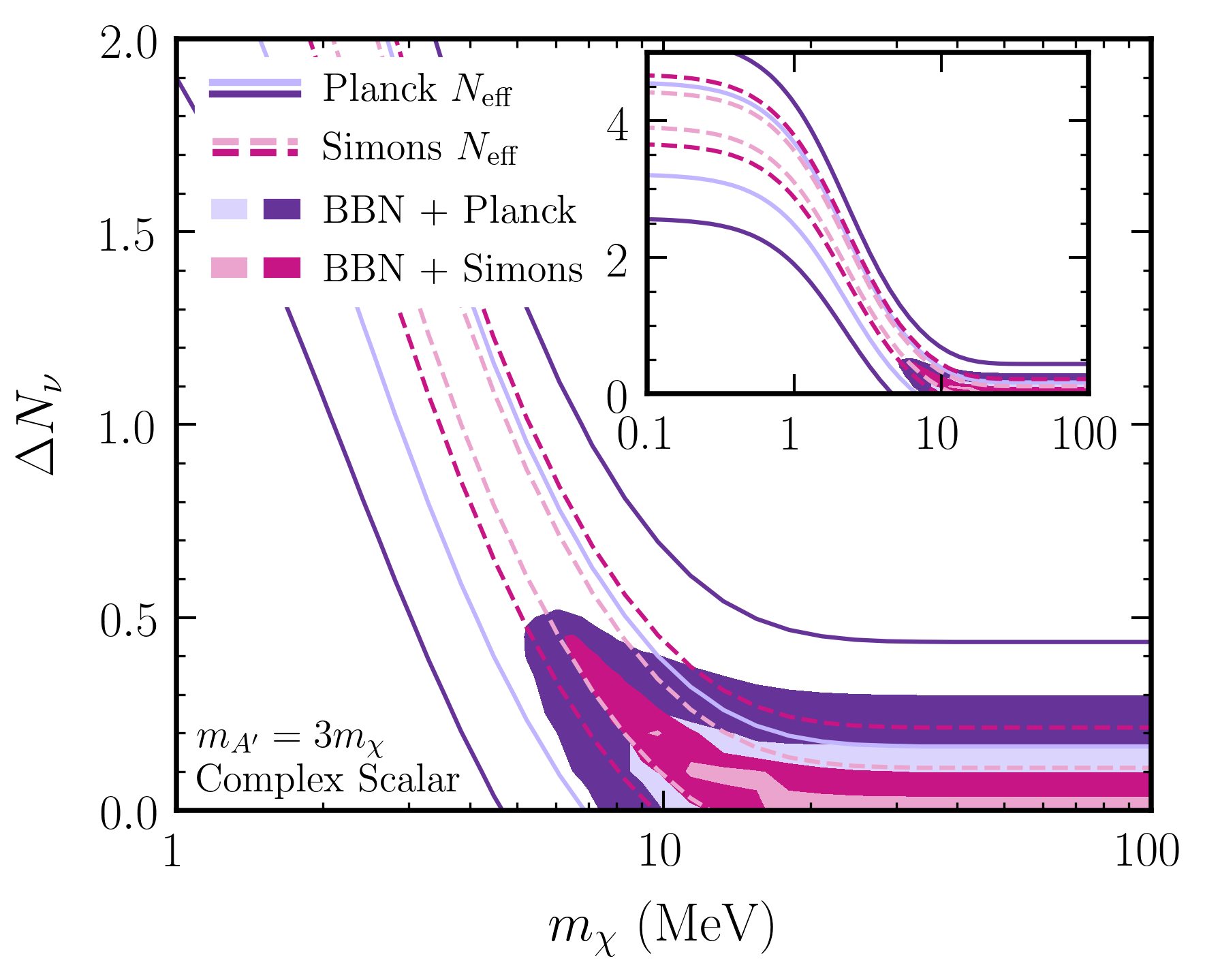
Figure 1: The allowed region of dark matter mass $m_{\chi}$ and $\Delta N_{\nu}$, for a complex scalar particle and a dark photon with mass $3m_{\chi}$. The inset shows the same contours over a larger range of $m_{\chi}$ and $\Delta N_{\nu}$. The purple (pink) lines denote the Planck (projected Simons Observatory) $N_{\rm eff}$ 68/95% confidence regions. The corresponding shaded regions correspond to the bounds including BBN measurements. The BBN measurements clearly play a powerful role in setting the lower limit on the dark matter mass, even when $\Delta N_{\nu}>0$ is allowed. The value of $\Omega_{b}h^{2}$ that maximizes the likelihood was chosen for each parameter point.

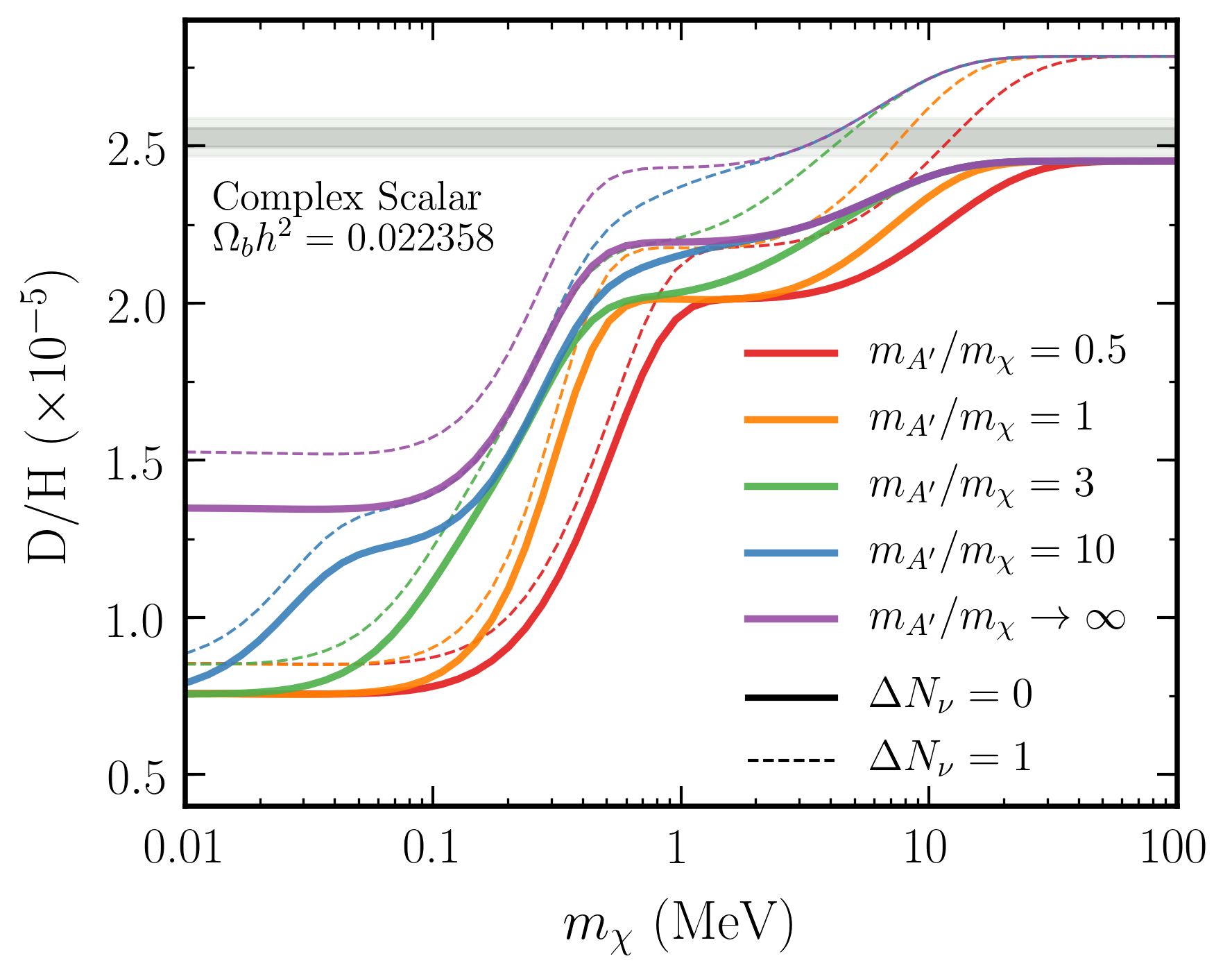
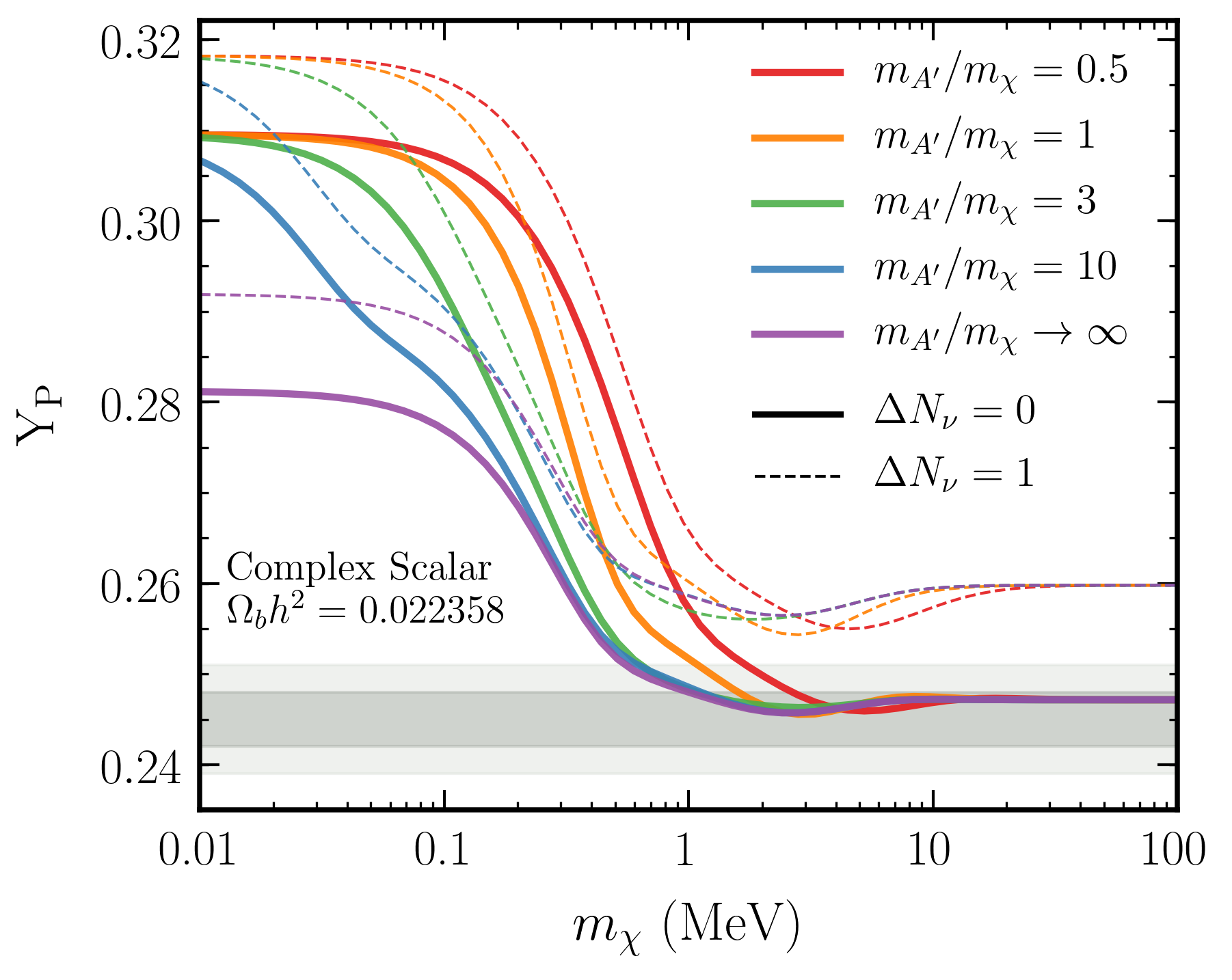
Figure 2: Predictions for D/H (left) and Y${}_{\textrm{P}}$ (right) for a complex scalar particle $\chi$ of mass $m_{\chi}$. The solid (dashed) lines correspond to $\Delta N_{\nu}=0~{}(1)$. The results are shown for five different ratios of dark photon to DM mass: $m_{A^{\prime}}/m_{\chi}=0.5,1,3,10$, and approaching $\infty$ in red, orange, green, blue, and purple, respectively. The 1 and 2$\sigma$ uncertainties on the measured values of D/H Cooke et al. (2018) and Y${}_{\textrm{P}}$ Zyla et al. (2020) are indicated by the gray horizontal bands. The standard cosmology predictions for D/H and Y_P are consistent with the results in Ref. Pitrou et al. (2021). $\Omega_{b}h^{2}$ is fixed to $0.022358$.

The contribution from BBN, $L_{\text{BBN}}$, is computed using the central values of the observed elemental abundances, and a covariance matrix that combines experimental and theoretical uncertainties. The measured values and uncertainties of Y${}_{\textrm{P}}$ Zyla et al. (2020) and D/H Cooke et al. (2018) are

$$\textrm{Y}_{\textrm{P}} = 0.245\pm 0.003\,,$$ (4)

D/H $$= (2.527\pm 0.030)\times 10^{-5}\,.$$

Theoretical uncertainties and correlations between predicted Y${}_{\text{P}}$ and D/H values arise from uncertainties in nuclear rates. The D/H theoretical uncertainty varies with both $\boldsymbol{\theta}$ and $\Omega_{b}h^{2}$, and can be comparable to or even exceed the measurement uncertainty; it is therefore evaluated at each parameter point. We compute the theoretical uncertainty and correlations of both D/H and Y${}_{\text{P}}$ by varying the nuclear rates by 1$\sigma$, and adding the resulting fractional variations to the abundances in quadrature. Finally, both theoretical and measurement uncertainties are added in quadrature to obtain the full BBN covariance matrix. Further details on this procedure are provided in Appendix B.

We then calculate the profile likelihood ratio $\lambda_{p}(\boldsymbol{\theta})=L_{p}(\boldsymbol{\theta})/\hat{L}_{p}$, where $L_{p}(\boldsymbol{\theta})=\max_{\Omega_{b}h^{2}}L(\boldsymbol{\theta},\Omega_{b}h^{2})$ and $\hat{L}_{p}=\max_{\boldsymbol{\theta},\Omega_{b}h^{2}}L(\boldsymbol{\theta},\Omega_{b}h^{2})$. By Wilk’s theorem, the quantity $-2\log\lambda_{p}(\boldsymbol{\theta})$ follows a chi-squared distribution with degrees of freedom given by the number of model parameters Zyla et al. (2020). 68 (95)% confidence limits for $\boldsymbol{\theta}$ in our two-parameter benchmark model are therefore set when $-2\log\lambda_{p}(\boldsymbol{\theta})=2.30~{}(6.18)$.

Dark Photon Model Constraints.—Fig. 1 illustrates the interplay between CMB and BBN measurements in constraining a complex scalar $\chi$ and a dark photon with $m_{A^{\prime}}=3m_{\chi}$. The purple (pink) lines correspond to the constraints on $m_{\chi}$ and $\Delta N_{\nu}$ that are consistent with the Planck (projected Simons Observatory) measurements. Above $m_{\chi}\sim 20$ MeV, the predicted value of $N_{\text{eff}}$  approaches the standard cosmological value because the DM freezes out well before neutrino decoupling, and so the DM annihilations heat the electromagnetic and neutrino sectors equally.

The impact of the dark sector becomes apparent when $m_{\chi}\lesssim$20\text{\,}\mathrm{Me\kern-0.50003ptV}$$, and entropy is injected into the electromagnetic sector during and after the period of neutrino decoupling, when the SM bath has a temperature of $T_{\nu d}\sim$2\text{\,}\mathrm{Me\kern-0.50003ptV}$$. In this case, $N_{\text{eff}}$  decreases relative to the standard value because the electromagnetic sector is preferentially heated, but the photon temperature today is fixed at its measured value of 2.7 K. A nonzero $\Delta N_{\nu}$ can restore $N_{\text{eff}}$  to its measured value; when $m_{\chi}$ falls below $\sim$20\text{\,}\mathrm{Me\kern-0.50003ptV}$$, the fit clearly prefers a larger $\Delta N_{\nu}$ to explain the observed value of $N_{\text{eff}}$. Below $m_{\chi}\lesssim$1\text{\,}\mathrm{Me\kern-0.50003ptV}$$, the DM is relativistic throughout neutrino decoupling, entropy is dumped only into the electromagnetic sector regardless of mass, and the constraints level off (Fig. 1 inset).

The result of including BBN constraints from Y${}_{\text{P}}$ and D/H is indicated by the shaded regions in Fig. 1. BBN clearly adds significant discriminating power, placing a 95% lower confidence bound on the DM mass of $m_{\chi}\sim$5\text{\,}\mathrm{Me\kern-0.50003ptV}$$ when combined with Planck data, regardless of $\Delta N_{\nu}$. The Simons Observatory will have improved sensitivity to $m_{\chi}$ with its more precise measurement of $N_{\text{eff}}$, while also reducing the uncertainty on $\Delta N_{\nu}$.

The introduction of an $\text{\,}\mathrm{Me\kern-0.50003ptV}$-scale DM particle and dark photon leads to a variety of effects on BBN physics, which are summarized in Fig. 2 for fixed $\Omega_{b}h^{2}=0.022358$. The solid (dashed) colored lines correspond to different ratios of $m_{A^{\prime}}/m_{\chi}$ for $\Delta N_{\nu}=$ 0 (1). The case where $m_{A^{\prime}}/m_{\chi}\rightarrow\infty$ is consistent with Refs. Kolb et al. (1986); Serpico and Raffelt (2004); Boehm et al. (2013); Nollett and Steigman (2014). The interplay of the following four quantities is relevant for understanding this behavior: i) the neutron-proton ratio, which is positively correlated with the helium-4 abundance, ii) the baryon-to-photon ratio, $\eta$, which is inversely correlated with the deuterium abundance, iii) the expansion rate, which impacts both the neutron abundance and the deuterium burning rate Mukhanov (2004), and iv) the rate of neutron-proton interconversion, affected by a modified $T_{\nu}$ (at fixed $T_{\gamma}$). When $m_{\chi}\gtrsim 3\,T_{\nu d}$, BBN proceeds as per the standard scenario. When $m_{e}\lesssim m_{\chi}\lesssim 3\,T_{\nu d}$, DM injects significant entropy into the electromagnetic sector after neutrino decoupling. The expansion rate is therefore slower at fixed photon temperature, which drives down the deuterium abundance as there is more time to convert deuterium to heavier elements. Meanwhile, near-cancellation of effects on neutron-proton interconversion and on the expansion rate keeps Y${}_{\textrm{P}}$ essentially constant in this regime Nollett and Steigman (2014). When $m_{\chi}\lesssim m_{e}$, the DM acts as a new relativistic species during BBN. This increases the expansion rate, causing weak interactions to decouple earlier, thereby increasing Y${}_{\textrm{P}}$. In contrast, D/H is further reduced because post-BBN DM annihilations lead to an increased $\eta$ during BBN.

$\Delta N_{\nu}>0$ compounds the effect of introducing an MeV-scale DM particle by further increasing the expansion rate. This increases the production of helium-4 and mitigates the decrease in the deuterium abundance. As a result, an increase in $\Delta N_{\nu}$ shifts the $\Delta N_{\nu}=0$ curves in Fig. 2 upwards.

As $m_{A^{\prime}}/m_{\chi}$ is reduced, the effects described above are only further enhanced because of the additional entropy injection from the dark photon. In particular circumstances, the presence of the dark photon can qualitatively affect the shape of the D/H and Y${}_{\textrm{P}}$ curves in Fig. 2. For example, the $m_{A^{\prime}}/m_{\chi}=10$ curve exhibits distinctive behavior when $m_{\chi}\lesssim m_{e}$. The observed plateau in D/H corresponds to the transition from the point where the dark photon entropy injection heats the photon bath, to the point where the dark photon acts as an additional relativistic species throughout BBN. Elsewhere, the curves for different values of $m_{A^{\prime}}/m_{\chi}$ look similar, but the curves shift to the right as $m_{A^{\prime}}/m_{\chi}$ decreases, since the entropy injection from the dark photon increases as $m_{A^{\prime}}$ decreases.

The current measurements of D/H and Y${}_{\textrm{P}}$ are indicated in Fig. 2. For the case where $m_{\chi}\rightarrow\infty$, we find a $\sim 2\sigma$ discrepancy with the measured deuterium abundance from Ref. Cooke et al. (2018), consistent with other studies using PRIMAT. Refs. Yeh et al. (2021); Pisanti et al. (2021), which perform independent analyses with different code packages, find better agreement with larger uncertainties. These differences are likely due, at least in part, to differing treatments of the 2D $\rightarrow$ ³He + n and 2D $\rightarrow$ ³H + p reactions Pisanti et al. (2021); Pitrou et al. (2021). The method presented in this Letter can be easily adapted to account for future improvements in BBN calculations.

Table 1 enumerates the 95% confidence lower bound on $m_{\chi}$ for a complex scalar, a Majorana fermion, and a Dirac fermion for different values of $m_{A^{\prime}}/m_{\chi}$. In all cases, the minimum mass is constant for $m_{A^{\prime}}/m_{\chi}\gtrsim 10$ and is a factor of 1.3–1.8 weaker than joint CMB and BBN limits assuming $\Delta N_{\nu}=0$ Sabti et al. (2021). We find a robust lower bound of $m_{\chi}>$3.9\text{\,}\mathrm{Me\kern-0.50003ptV}$$ across all DM particle types, for any non-zero $\Delta N_{\nu}$, using Planck data Aghanim et al. (2020). The Simons Observatory will be sensitive to heavier masses by several $\text{\,}\mathrm{Me\kern-0.50003ptV}$.

The lower bound on $m_{\chi}$ has important implications for experiments searching for dark sector DM. Our benchmark model is commonly used to present bounds and sensitivity projections for direct-detection and accelerator-based experiments. To date, the generality of CMB $N_{\text{eff}}$ limits on this model has been questioned due to the degeneracy between DM entropy injection and $\Delta N_{\nu}$ Boehm et al. (2013); Essig et al. (2016); Wilkinson et al. (2016); Izaguirre et al. (2017); Berlin et al. (2019). Because our joint CMB and BBN constraints apply for any $\Delta N_{\nu}>0$, they address these prior concerns and establish a robust cosmological bound on the dark sector model under consideration.

	Minimum $\boldsymbol{m_{\chi}}$ [MeV]
$m_{A^{\prime}}/m_{\chi}$	Complex Scalar	Majorana Fermion	Dirac    Fermion
0.5	14.3  (16.5)	14.3  (16.5)	15.2  (17.1)
1	9.0  (10.1)	9.0  (10.1)	10.4  (11.5)
1.5	7.1  (8.1)	7.1  (8.0)	9.0  (10.0)
3	5.2  (6.2)	5.0  (6.1)	7.9  (9.1)
$\geq 10$	4.3  (5.8)	4.0  (5.6)	7.8  (9.1)

Table 1: The joint Planck CMB and BBN 95% lower limit on the mass of a DM particle that is a complex scalar, Majorana fermion, or Dirac fermion in our benchmark model. The mass limits are provided for different ratios of the dark photon to DM mass. The values in parentheses are the projected Simons Observatory and BBN constraints Ade et al. (2019); Sabti et al. (2020). The value of $\Omega_{b}h^{2}$ that maximizes the likelihood was chosen for each parameter point.

We present our results in Fig. 3 for $m_{A^{\prime}}=3m_{\chi}$ in terms of the reference DM-electron scattering cross section, $\overline{\sigma}_{e}\equiv 16\pi\alpha\alpha_{D}\epsilon^{2}\mu_{\chi e}^{2}/(\alpha^{2}m_{e}^{2}+m_{A^{\prime}}^{2})^{2}$, where $\alpha$, $\alpha_{D}$ are the electromagnetic and dark sector fine structure constants respectively, $\epsilon$ is the SM-$A^{\prime}$ mixing parameter, and $\mu_{\chi e}$ is the electron-$\chi$ reduced mass. We show the lower limit on $m_{\chi}$ for a Dirac fermion and a complex scalar, together with existing direct-detection Essig et al. (2012, 2017); Agnes et al. (2018); Aprile et al. (2019); Barak et al. (2020); Cheng et al. (2021) and accelerator Adler et al. (2002); Artamonov et al. (2009); deNiverville et al. (2011); Batell et al. (2014); Banerjee et al. (2019); Lees et al. (2017) limits on $\overline{\sigma}_{e}$, assuming $\chi$ makes up all of the DM for direct-detection experiments, and choosing $\alpha_{D}=0.5$ for beam experiments. We solve the Boltzmann equation for $\chi$ with the processes $\chi\overline{\chi}\leftrightarrow e^{+}e^{-}$ and $\mu^{+}\mu^{-}$ to obtain i) $\overline{\sigma}_{e}$ as a function of $m_{\chi}$ for a symmetric complex scalar $\chi$ undergoing a standard freezeout through annihilation into SM fermions, and ii) the lower limit on $\overline{\sigma}_{e}$ as a function of $m_{\chi}$ for an asymmetric Dirac fermion $\chi$ freezing out through annihilation into SM fermions, given the Planck limits on DM annihilation Lin et al. (2012); Slatyer (2016); Aghanim et al. (2020) (see, e.g., Refs. Steigman et al. (2012); Feng and Smolinsky (2017); Berlin et al. (2019) for similar relic abundance calculations). The joint constraints set a lower limit of $m_{\chi}>$5.2\text{\,}\mathrm{Me\kern-0.50003ptV}$$ ($7.9\text{\,}\mathrm{Me\kern-0.50003ptV}$) for a complex scalar (Dirac fermion) $\chi$ with an arbitrary number of light degrees of freedom at 95% confidence. The Simons Observatory Ade et al. (2019); Sabti et al. (2020) is forecasted to have slightly improved sensitivity.

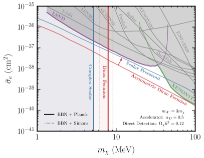
Figure 3: Joint CMB and BBN 95% confidence constraints on $m_{\chi}$ when $\chi$ is a Dirac fermion (shaded red) or a complex scalar (shaded blue), with $m_{A^{\prime}}=3m_{\chi}$. The $y$-axis shows the reference dark matter-electron scattering cross section $\overline{\sigma}_{e}$. Projected constraints from the Simons Observatory are demarcated by the vertical dotted lines. The blue line indicates where a complex scalar $\chi$ undergoes a standard freezeout to attain the correct relic abundance; the line above which the freezeout of an asymmetric Dirac fermion $\chi$ can produce all of DM is indicated in red. The region of parameter space that is ruled out by experiments at the 90% confidence level is shaded grey, with the strongest constraints coming from LSND deNiverville et al. (2011) (purple) and XENON1T Aprile et al. (2019) (green). Other experimental limits are shown as labeled gray lines Adler et al. (2002); Artamonov et al. (2009); Essig et al. (2012); Banerjee et al. (2019); Lees et al. (2017); Essig et al. (2017); Agnes et al. (2018); Barak et al. (2020); Cheng et al. (2021). All direct-detection limits on $\overline{\sigma}_{e}$ assume $\chi$ is all of the DM, while accelerator-based limits are independent of the $\chi$-abundance, but assume $\alpha_{D}=0.5$.

Our limits apply only for dark sectors in chemical equilibrium with the SM while $A^{\prime}$ is relativistic, where our entropy injection calculation is valid. In the early Universe, processes such as $\chi\overline{\chi}\leftrightarrow e^{+}e^{-}$ bring the dark sector into chemical equilibrium with the SM while $T_{\gamma}\gtrsim m_{A^{\prime}}$ for sufficiently large $\overline{\sigma}_{e}$. We estimate this $\overline{\sigma}_{e}$ by requiring the rate of $e^{+}e^{-}\to\chi\overline{\chi}$ to exceed the Hubble rate at $T_{\gamma}=m_{A^{\prime}}$, and find $\overline{\sigma}_{e}\gtrsim${10}^{-46}\text{\,}{\mathrm{cm}}^{2}$($10\text{\,}\mathrm{Me\kern-0.50003ptV}$/m_{\chi})^{3}$.

Conclusions.— We have developed a method for obtaining joint CMB and BBN constraints on general dark sectors. As a concrete example, we focused on the dark sector model where a DM particle interacts with the SM through a massive dark photon mediator, including the possibility of an arbitrary number of light degrees of freedom. We place a 95% confidence lower bound of $m_{\chi}\gtrsim$4\text{\,}\mathrm{Me\kern-0.50003ptV}$$ on the DM mass as long as the dark sector is fully thermalized with the SM in the early Universe. In Table 1, we also illustrate how the constraints strengthen with decreasing dark photon mass. Recent studies have identified cosmological and astrophysical probes of $\chi e\rightarrow\chi e$ scattering Buen-Abad et al. (2021); Nguyen et al. (2021), resulting in constraints on $\bar{\sigma}_{e}$ that are many orders of magnitude weaker than the range plotted in Fig. 3 (e.g., $\overline{\sigma}_{e}\gtrsim${10}^{-30}\text{\,}{\mathrm{cm}}^{2}$$ for $m_{\chi}=$1\text{\,}\mathrm{Me\kern-0.50003ptV}$$). Thus, for the example of $m_{\chi}=$1\text{\,}\mathrm{Me\kern-0.50003ptV}$$, our constraints are expected to apply between $${10}^{-43}\text{\,}{\mathrm{cm}}^{2}$\lesssim\overline{\sigma}_{e}\lesssim${10}^{-30}\text{\,}{\mathrm{cm}}^{2}$$, above which $\chi e\to\chi e$ becomes important. To our knowledge, there are no existing models of electrophilic DM that completely evade our bounds, though model-building extensions have been proposed for other scenarios that can weaken the CMB $N_{\text{eff}}$ constraints and allow for $110\text{\,}\mathrm{Me\kern-0.50003ptV}$ electromagnetically-coupled dark sector particles, e.g., by allowing some DM annihilation into neutrinos Escudero (2019); Sabti et al. (2020); Agashe et al. (2021). We hope to better understand the robustness of these cosmological limits on generic dark sectors in future work.

Appendices C and D describe the modifications made to nudec_BSM and PRIMAT to handle the dark sector model studied in this Letter. The modified code is available upon request from the authors.

Acknowledgements.—The authors thank Kaustubh Agashe, Alexandre Arbey, Asher Berlin, Kimberly Boddy, Manuel Buen-Abad, Bhaskar Dutta, Rouven Essig, Jonathan Feng, Vera Gluscevic, David McKeen, Siddharth Mishra-Sharma, Cyril Pitrou, Maxim Pospelov, Jordan Smolinsky, Yuhsin Tsai, Neal Weiner, Tien-Tien Yu and Yiming Zhong for fruitful conversations. This material is based upon work supported by the NSF Graduate Research Fellowship under Grant No. DGE1839302. HL and ML are supported by the DOE under Award Number DE-SC0007968. ML is also supported by the Cottrell Scholar Program through the Research Corporation for Science Advancement. HL is also supported by NSF grant PHY-1915409, and the Simons Foundation. JTR is supported by NSF CAREER grant PHY-1554858 and NSF grant PHY-1915409. This work was performed in part at the Aspen Center for Physics, which is supported by NSF grant PHY-1607611. The work presented in this paper was performed on computational resources managed and supported by Princeton Research Computing. This research made extensive use of the publicly available codes nudec_BSM Escudero (2019); Escudero Abenza (2020) and PRIMAT Pitrou et al. (2018, 2021), as well as the IPython (Perez and Granger, 2007), Jupyter (Kluyver et al., 2016), matplotlib (Hunter, 2007), NumPy (van der Walt et al., 2011), and SciPy (Jones et al., 2001) software packages.

oneΔ

Appendix A $N_{\text{eff}}$ Constraint

This appendix provides a pedagogical derivation of $N_{\text{eff}}$  as a function of $m_{\chi}$ in the presence of a dark matter (DM) particle $\chi$ and a dark photon $A^{\prime}$. We assume that neutrino decoupling is instantaneous in this appendix so that the results are analytical; however, the results in the main Letter include corrections for non-instantaneous neutrino decoupling, obtained using the modified nudec_BSM code described in Appendices C and D.

Our goal is to use conservation of entropy to determine the increase in photon temperature due to DM freezeout. The entropy density of a given species $i$ is defined as

$$s_{i}=\frac{\rho_{i}+P_{i}}{T_{i}}\,,$$

where $\rho_{i}$ is the energy density, $P_{i}$ is the pressure, and $T_{i}$ is the temperature of species $i$. For the benchmark dark sector considered in this work, the total radiation density of the early Universe is given by

$$\rho_{R}=\rho_{\gamma}+\rho_{e}+3\rho_{\nu}+\rho_{\xi}+\rho_{\chi}+\rho_{A^{\prime}}\,,$$

where we have included the energy density of additional light degrees of freedom $\xi$, in addition to the contribution from photons, electrons/positrons, neutrinos, $\chi$, and $A^{\prime}$. The energy density of species $i$ with energy $E_{i}(p)$ is given by

$$\rho_{i}(E_{i})=\frac{g_{i}}{2\pi^{2}}\int_{0}^{\infty}\textrm{d}p\,f_{i}(p)\,E_{i}(p)\,p^{2}\,,$$

where the distribution function $f_{i}(p)$ is either Bose-Einstein or Fermi-Dirac, and $g_{i}$ corresponds to the internal degrees of freedom of the particle (i.e., 1 for a real scalar, 2 for a complex scalar or Majorana fermion, and 4 for a Dirac fermion). Taking $E_{i}(p)=\sqrt{p^{2}+m_{i}^{2}}$ and substituting in for $f_{i}(p)$ yields

$$\rho_{i}(m_{i},T_{i})=\frac{g_{i}}{2\pi^{2}}\int_{0}^{\infty}\,\textrm{d}p\,\frac{p^{2}\sqrt{p^{2}+m_{i}^{2}}}{e^{\sqrt{p^{2}+m_{i}^{2}}/T_{i}}\pm 1}\,.$$

For notational convenience, we change variables to $x_{i}\equiv m_{i}/T_{i}$ and $\lambda_{i}\equiv p/T_{i}$, so that the energy density becomes

$$\rho_{i}(x_{i})=\frac{g_{i}}{2\pi^{2}}\,T_{i}^{4}\,J_{\pm}(x_{i})\,\,,$$ (A1)

where

$$J_{\pm}(x)\equiv\int_{0}^{\infty}\differential\lambda\,\frac{\lambda^{2}\sqrt{\lambda^{2}+x^{2}}}{e^{\sqrt{\lambda^{2}+x^{2}}}\pm 1}\,.$$

Meanwhile, the pressure of species $i$ is given by

$$P_{i}(E_{i})=\frac{g_{i}}{(2\pi)^{2}}\int_{0}^{\pi}\differential\theta\sin\theta\int_{0}^{\infty}\textrm{d}p\,f_{i}(p)\,\frac{p^{2}}{3E_{i}(p)}\,p^{2}\,,$$

which can be rewritten as

$$P_{i}(x_{i})=\frac{g_{i}}{2\pi^{2}}\,T_{i}^{4}\int_{0}^{\infty}\differential\lambda\,\frac{\lambda^{4}}{3\sqrt{\lambda^{2}+x_{i}^{2}}}\frac{1}{e^{\sqrt{\lambda^{2}+x_{i}^{2}}}\pm 1}\,.$$ (A2)

The total entropy density is therefore

$$s_{\textrm{tot}}=\sum_{i}\frac{g_{i}}{2\pi^{2}}\,T^{3}_{i}\left[J_{\pm}(x_{i})+\int_{0}^{\infty}\differential\lambda\,\frac{\lambda^{4}}{3\sqrt{\lambda^{2}+x_{i}^{2}}}\frac{1}{e^{\sqrt{\lambda^{2}+x_{i}^{2}}}\pm 1}\right]\,.$$ (A3)

For light or massless species ($x_{i}\ll 1$), Eq. (A3) can be further simplified because $J_{\pm}(x)$ can be evaluated analytically in the relativistic limit. In this case,

$$J_{+}(0)=\frac{7\pi^{4}}{120}\quad\text{ and }\quad J_{-}(0)=\frac{\pi^{4}}{15}\,,$$

which gives

$$\rho_{i}(0)=\frac{\pi^{2}}{30}\,g_{i}\,T_{i}^{4}\times\begin{cases}1&\text{for bosons}\\ \frac{7}{8}&\text{for fermions}\,.\\ \end{cases}$$ (A4)

We define

$$g_{*}(T_{\gamma})\equiv\sum_{i\in\textrm{bosons}}g_{i}\left(\frac{T_{i}}{T_{\gamma}}\right)^{4}+\frac{7}{8}\sum_{i\in\textrm{fermions}}g_{i}\left(\frac{T_{i}}{T_{\gamma}}\right)^{4},$$

where $T_{\gamma}$ is the photon temperature, such that the total energy density of all relativistic SM species and DM is

$$\rho_{\textrm{tot,rel}}=\frac{\pi^{2}}{30}\,T_{\gamma}^{4}\,g_{*}(T_{\gamma})\,.$$

The expression for pressure also simplifies in this limit; taking $x\rightarrow 0$ in the relativistic limit, we find

$$P_{i}(0)=\frac{g_{i}}{6\pi^{2}}\,T_{i}^{4}\int_{0}^{\infty}\textrm{d}\lambda\,\frac{\lambda^{3}}{e^{\lambda}\pm 1}=\frac{1}{3}\,\rho_{i}(0)\,,$$

returning the expected relation for a relativistic gas. The total entropy density for relativistic species then becomes

$$s_{\textrm{tot,rel}}=\frac{4}{3}\sum_{i}\frac{\rho_{i}(0)}{T_{i}}=\frac{2\pi^{2}}{45}\,T_{\gamma}^{3}\left[\sum_{i\in\textrm{bosons}}g_{i}\left(\frac{T_{i}}{T_{\gamma}}\right)^{3}+\frac{7}{8}\sum_{i\in\textrm{fermions}}g_{i}\left(\frac{T_{i}}{T_{\gamma}}\right)^{3}\right]\,.$$ (A5)

We can simplify this expression by defining

$$g_{*S}(T_{\gamma})\equiv\sum_{i\in\textrm{bosons}}g_{i}\left(\frac{T_{i}}{T_{\gamma}}\right)^{3}+\frac{7}{8}\sum_{i\in\textrm{fermions}}g_{i}\left(\frac{T_{i}}{T_{\gamma}}\right)^{3}$$

such that Eq. (A5) becomes

$$s_{\textrm{tot,rel}}=\frac{2\pi^{2}}{45}\,T_{\gamma}^{3}\,g_{*S}(T_{\gamma})\,.$$ (A6)

To find the total entropy density including contributions from nonrelativistic species, we must evaluate the integrals in Eq.(A3) numerically.

Now that we have an expression for entropy density as a function of temperature and particle mass, we can use conservation of entropy to determine the photon heating from DM freeze out. We assume that electrons, photons, and DM are in thermal equilibrium until they decouple from the SM plasma. At the point of neutrino decoupling, the total entropy density of all radiative species

$$s_{\textrm{tot}}\big{|}_{a_{d}}=\frac{2\pi^{2}}{45}\,T_{\nu d}^{3}\left[g_{\gamma}+\frac{7}{8}\big{(}g_{e}\phi(x_{ed})+3g_{\nu}\big{)}+\tilde{g}_{\chi}\phi(x_{\chi d})+g_{A^{\prime}}\phi(x_{A^{\prime}d})\right]+\frac{2\pi^{2}}{45}T^{3}_{\xi,a_{d}}\tilde{g}_{\xi}\,,$$ (A7)

where $T_{\nu d}$ is the common temperature of all SM species and dark sector species at the point of neutrino decoupling, which occurs at the corresponding scale factor $a_{d}$, and

$$\phi(x_{id})\equiv\frac{s_{i}(x_{id})}{s_{i}(0)}\,,$$

where $x_{id}\equiv m_{i}/T_{\nu d}$ for species $i$. Following Ref. Nollett and Steigman (2015), we have introduced the notation $\tilde{g}_{\chi}$ to absorb fermion factors of 7/8 for particles with different numbers of degrees of freedom, i.e., $\tilde{g}_{\chi}=1,\,7/4,\,2$, and $7/2$ for a real scalar, Majorana fermion, complex scalar, and Dirac fermion, respectively. We also include a term $\tilde{g}_{\xi}$ to parametrize the entropy contributed by equivalent neutrinos (which also may have additional fermion factors attached), as well as the temperature of the equivalent neutrinos at the point of neutrino decoupling $T_{\xi,a_{d}}$, which is not necessarily the temperature of the SM plasma.

After some time, the DM and the positrons/electrons annihilate, injecting energy into the photon bath. DM annihilations that occur after neutrino decoupling inject entropy into the electromagnetic plasma only, thereby increasing $T_{\gamma}$; the same occurs during electron-positron annihilation. In this Appendix, we assume that $e^{+}e^{-}$ annihilation occurs entirely after neutrinos have decoupled, so that all of the annihilations heat the electromagnetic sector and our calculations remain analytical. In reality, there is some overlap between neutrino decoupling and electron-positron annihilation that causes neutrinos to be slightly heated by this process as well; this effect is tracked numerically in the main Letter. To track temperature evolution during these processes, we separately conserve entropy among all species coupled to photons (photons, electrons, DM and dark photons), and among all species that do not receive an energy injection from electron-positron annihilation or DM freeze out. This means that, at some reference value of the scale factor $a=a_{2}$ after electron-positron annihilation and DM freeze out, the total entropy is given by

$$s_{\textrm{tot}}\big{|}_{a_{2}}=\frac{2\pi^{2}}{45}\left[g_{\gamma}T_{\gamma,a_{2}}^{3}+\frac{21}{8}g_{\nu}T_{\nu,a_{2}}^{3}+g_{\xi}T^{3}_{\xi,a_{2}}\right]\,,$$ (A8)

where $T_{\gamma,a_{2}}\neq T_{\nu,a_{2}}$ because photons are heated after neutrino decoupling. Because neutrinos decouple completely before any other species freezes out in this approximation, we expect $T_{\nu}$ to scale as $a^{-1}$, i.e., $a_{d}T_{\nu d}=a_{2}T_{\nu,a_{2}}$. A similar relation holds for the equivalent neutrino temperature. Equating the total entropy before and after electron-positron annihilation and DM freeze out then yields

$$g_{\gamma}+\frac{7}{2}\phi(x_{ed})+\frac{21}{8}g_{\nu}+\tilde{g}_{\chi}\phi(x_{\chi d})+g_{A^{\prime}}\phi(x_{A^{\prime}d})+g_{\xi}=\left(\frac{T_{\gamma}}{T_{\nu}}\right)_{0}^{3}g_{\gamma}+\frac{21}{8}g_{\nu}+g_{\xi}\,,$$

or

$$\left(\frac{T_{\nu}}{T_{\gamma}}\right)^{3}_{0}=\frac{g_{\gamma}}{g_{\gamma}+\frac{7}{2}\phi(x_{ed})+\tilde{g}_{\chi}\phi(x_{\chi d})+g_{A^{\prime}}\phi(x_{A^{\prime}d})}\,.$$ (A9)

We use the subscript ‘0’ to denote a late point in time when $T_{\gamma}\ll m_{\chi}$, $m_{A^{\prime}}$, and $m_{e}$. Knowing the late-time ratio of the neutrino and photon temperatures, we can also use Eq. (A4) to find the ratio of their radiation densities. This allows us to find the effective number of relativistic degrees of freedom,

$$N_{\textrm{eff}}\equiv\left(\frac{\rho_{R}-\rho_{\gamma}}{\rho_{\nu,\textrm{std}}}\right)_{0}\,.$$ (A10)

Here, the subscript “std” denotes the standard result (i.e., ignoring contributions from DM freeze out or other dark sector effects), including the assumption of i) instantaneous neutrino decoupling, and ii) no heating of the neutrinos from electrons and positrons. Using Eq. (A4), we may write this as

$$\left(\rho_{\nu,\textrm{std}}\right)_{0}=\frac{7}{8}\left(\frac{T_{\nu}}{T_{\gamma}}\right)_{0,\textrm{std}}^{4}\left(\rho_{\gamma}\right)_{0}=\frac{7}{8}\left(\frac{4}{11}\right)^{4/3}\left(\rho_{\gamma}\right)_{0},$$

where we have used expressions similar to Eqs. (A7) and (A8) to find the ratio of the photon and neutrino temperatures under the assumptions listed above (see Dodelson (2003)). We can also write

$$\left(\frac{\rho_{R}}{\rho_{\gamma}}\right)_{0} =1+\left(\frac{3\rho_{\nu}}{\rho_{\gamma}}\right)_{0}+\left(\frac{\rho_{\xi}}{\rho_{\gamma}}\right)_{0}$$

$$=1+\left(\frac{\rho_{\nu}}{\rho_{\gamma}}\right)_{0}\big{(}3+\Delta N_{\nu}\big{)},$$ (A11)

with $\Delta N_{\nu}\equiv\left(\frac{\rho_{\xi}}{\rho_{\nu}}\right)_{0}$ as the number of equivalent neutrinos in the early Universe. With the result from Eq. (A9), $N_{\text{eff}}$ is given by

$$N_{\textrm{eff}}=3\left(\frac{11}{4}\frac{g_{\gamma}}{g_{\gamma}+\frac{7}{2}\phi(x_{ed})+\tilde{g}_{\chi}\phi(x_{\chi d})+g_{A^{\prime}}\phi(x_{A^{\prime}d})}\right)^{4/3}\left(1+\frac{\Delta N_{\nu}}{3}\right).$$ (A12)

This provides an analytical expression to find $N_{\text{eff}}$  in the presence of DM with mass $m_{\chi}$ and a dark photon with mass $m_{A^{\prime}}$. This result can be easily extended to accommodate richer dark sectors. In order to account for additional corrections from non-instantaneous neutrino decoupling and from QED, numerical tools are required; the modifications made to nudec_BSM to accomplish this are detailed in Appendix C. This code eliminates any need for an assumption of instantaneous neutrino decoupling by explicitly tracking the photon and neutrino temperatures as a function of time with a pair of coupled Boltzmann equations, taking into account collisions that occur between electrons and neutrinos and calculating the resulting energy transfer between the two sectors as neutrinos decouple over a finite period of time Escudero (2019).

Appendix B Treatment of CMB and BBN Covariances

In this appendix, we detail how to obtain the joint CMB and BBN constraints outlined in the main body. Starting from any dark sector model with some model parameters $\boldsymbol{\theta}$, we compute the overall effect of the dark sector on i) $N_{\text{eff}}$, the effective number of relativistic degrees of freedom at late times, and ii) the primordial abundances of elements after the process of BBN has ended. For each dark sector model, we perform the abundance calculations over the range $\Omega_{b}h^{2}\in[0.0218,0.0226]$, which is much broader than the Planck uncertainty on this parameter Aghanim et al. (2020). We leave a discussion of how to implement this procedure using existing numerical codes to the following section, simply assuming for now that the parameters $N_{\text{eff}}(\boldsymbol{\theta})$, $\textrm{Y}_{\textrm{P}}(\boldsymbol{\theta},\Omega_{b}h^{2})$, and D/H$(\boldsymbol{\theta},\Omega_{b}h^{2})$ can be obtained, together with theoretical uncertainties and correlations affecting the BBN calculation.

To assess the consistency of a given dark sector model with experimental measurements of primordial elemental abundance and the CMB, we perform a hypothesis test on our model parameters by constructing a profile likelihood ratio, as discussed in the main text. We define

$$L(\boldsymbol{\theta},\Omega_{b}h^{2})=L_{\text{BBN}}(\boldsymbol{\theta},\Omega_{b}h^{2})\cdot L_{\text{CMB}}(\boldsymbol{\theta},\Omega_{b}h^{2})\,,$$ (B1)

where $L$ is the Gaussian likelihood of the parameters $\boldsymbol{\theta}$ and $\Omega_{b}h^{2}$. The CMB contribution is

$$-2\log L_{\text{CMB}}(\boldsymbol{\theta},\Omega_{b}h^{2})=\left(\mathbf{x}(\boldsymbol{\theta},\Omega_{b}h^{2})-\hat{\mathbf{x}}\right)^{\intercal}\mathsf{C}_{\text{CMB}}^{-1}\left(\mathbf{x}(\boldsymbol{\theta},\Omega_{b}h^{2})-\hat{\mathbf{x}}\right)\,,$$ (B2)

where $\mathbf{x}(\boldsymbol{\theta},\Omega_{b}h^{2})\equiv(\Omega_{b}h^{2},N_{\text{eff}}(\boldsymbol{\theta}),\textrm{Y}_{\textrm{P}}(\boldsymbol{\theta}))^{\intercal}$, $\hat{\mathbf{x}}$ is the central value of the same parameters as reported by Planck Aghanim et al. (2020), and $\mathsf{C}$ is the reported covariance matrix for the three parameters we are considering. We use the base_nnu_yhe_plikHM_TTTEEE_lowl_lowE_post_BAO_lensing dataset, which fits for both $N_{\text{eff}}$ and Y${}_{\text{P}}$, in addition to the six $\Lambda$CDM parameters. For this dataset,

$$\hat{\mathbf{x}}\equiv(\Omega_{b}h^{2},N_{\text{eff}},\textrm{Y}_{\textrm{P}})_{\text{Planck}}=(0.022358,2.93,0.244)\,,\qquad\mathsf{C}_{\text{CMB}}=\begin{bmatrix}3.6\times 10^{-8}&1.5\times 10^{-5}&9.3\times 10^{-7}\\ 1.5\times 10^{-5}&8.2\times 10^{-2}&-3.5\times 10^{-3}\\ 9.3\times 10^{-7}&-3.5\times 10^{-3}&3.2\times 10^{-4}\end{bmatrix}\,.$$ (B3)

The BBN contribution is similarly constructed as

$$-2\log L_{\text{BBN}}(\boldsymbol{\theta},\Omega_{b}h^{2})=\left(\mathbf{y}(\boldsymbol{\theta},\Omega_{b}h^{2})-\hat{\mathbf{y}}\right)^{\intercal}\mathsf{C}_{\text{BBN}}^{-1}(\boldsymbol{\theta},\Omega_{b}h^{2})\left(\mathbf{y}(\boldsymbol{\theta},\Omega_{b}h^{2})-\hat{\mathbf{y}}\right)\,,$$ (B4)

where $\mathbf{y}(\boldsymbol{\theta},\Omega_{b}h^{2})\equiv(\textrm{Y}_{\textrm{P}}(\boldsymbol{\theta},\Omega_{b}h^{2}),\text{D/H}(\boldsymbol{\theta},\Omega_{b}h^{2}))^{\intercal}$, and $\hat{\mathbf{y}}$ is the vector of observed central values of Y${}_{\textrm{P}}$ Zyla et al. (2020) and D/H Cooke et al. (2018), given by $\hat{\mathbf{y}}=(0.245,2.527\times 10^{-5})^{\intercal}$. We use our modified version of PRIMAT Pitrou et al. (2018) to compute $\mathbf{y}(\boldsymbol{\theta},\Omega_{b}h^{2})$. Unlike the CMB covariance matrix, the BBN covariance $\mathsf{C}_{\text{BBN}}(\boldsymbol{\theta},\Omega_{b}h^{2})$ depends on both the model parameters and baryon density. There are two contributions: i) uncertainties in the measurement of Y${}_{\textrm{P}}$ and D/H, $\sigma_{\textrm{Y}_{\textrm{P}}}^{\text{ex}}$ and $\sigma_{\text{D/H}}^{\text{ex}}$, which can be straightforwardly obtained from the quoted measurement uncertainties in Refs. Zyla et al. (2020); Cooke et al. (2018), and ii) theoretical uncertainties in the computation of elemental abundances as a function of $\boldsymbol{\theta}$ and $\Omega_{b}h^{2}$ due to uncertainties in nuclear rates, which depend on $\boldsymbol{\theta}$ and $\Omega_{b}h^{2}$.

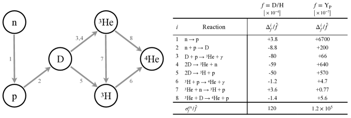
Figure B1: (Left, the piscis) The reactions in the BBN network that contribute most significantly to the theoretical uncertainties in the D/H and Y${}_{\textrm{P}}$ predictions, assuming the standard cosmological scenario ($m_{\chi}\rightarrow\infty$). Each reaction is labeled by an index $i$ (gray number), which is specified in the associated table. (Right)  The table shows the fractional change in the D/H and Y${}_{\textrm{P}}$ predictions, relative to the central measured values provided in Eq. (4), that we obtain by varying the rate of reaction $i$ within $1\sigma^{\rm th}_{i}$ of its theoretical uncertainty. Importantly, the theoretical uncertainty $\sigma^{\rm th}_{i}$ depends on both the model parameters $\boldsymbol{\theta}$ as well as $\Omega_{b}h^{2}$. The values in this table correspond to the standard cosmological scenario with $\Omega_{b}h^{2}=0.022358$, and will change for different regions of dark sector parameter space, although we find that they always remain $\lesssim 1.3\%$. For comparison, the bottom row of the table includes the relative size of the measurement uncertainty in the D/H and Y${}_{\textrm{P}}$ abundances, compared to their respective central values. Note that the uncertainty of proton-neutron interconversion is dominated by the uncertainty in the neutron lifetime Pitrou et al. (2018).

To estimate the theoretical uncertainties, we follow the method described in Refs. Fiorentini et al. (1998); Arbey et al. (2016) and implemented in the public BBN code AlterBBN Arbey (2012); Arbey et al. (2020) to calculate the covariances through variation of the reaction rates. Specifically, we compare the predicted BBN abundances using the central values for each reaction rate versus the predictions when the $i^{\text{th}}$ reaction rate in the network is increased to the central value plus its quoted theoretical uncertainity, $\sigma^{\text{th}}_{i}(\boldsymbol{\theta},\Omega_{b}h^{2})$, which in general varies with the photon temperature. This gives rise to a change to the elemental abundances $\Delta_{f}^{i}$, where $f$ is either Y${}_{\textrm{P}}$ or D/H. Fig. B1 shows the eight reactions that give the largest shift to the fractional abundances of D/H and Y_P, assuming the standard cosmological scenario with $m_{\chi}\rightarrow\infty$. Because all reaction rates lead to a small ($\lesssim 1$%) change in $\Delta_{f}^{i}/\hat{f}$, we can approximate the uncertainties in the predicted abundances as linear and add them in quadrature, i.e.,

$$\sigma_{\textrm{Y}_{\textrm{P}}}^{\text{th}}(\boldsymbol{\theta},\Omega_{b}h^{2})=\left[\sum_{i}(\Delta_{\textrm{Y}_{\textrm{P}}}^{i})^{2}\right]^{1/2}\,,\quad\sigma_{\text{D/H}}^{\text{th}}(\boldsymbol{\theta},\Omega_{b}h^{2})=\left[\sum_{i}(\Delta_{\text{D/H}}^{i})^{2}\right]^{1/2}\,,\quad\tau^{\text{th}}(\boldsymbol{\theta},\Omega_{b}h^{2})=\sum_{i}\Delta^{i}_{\textrm{Y}_{\textrm{P}}}\Delta^{i}_{\text{D/H}}\,,$$ (B5)

where $\tau\equiv\text{cov}(\textrm{Y}_{\textrm{P}},\text{D/H})$ is the covariance between Y${}_{\textrm{P}}$ and D/H, and the sum $i$ is over the eight reactions shown in Fig. B1. Without any electromagnetically interacting DM and taking the central value of $\Omega_{b}h^{2}=0.022358$ in our Planck dataset, these quantities as computed by our modified version of PRIMAT are

$$\sigma_{\textrm{Y}_{\textrm{P}}}^{\text{th},\Lambda\text{CDM}}=1.7\times 10^{-4}\quad,\quad\sigma_{\text{D/H}}^{\text{th},\Lambda\text{CDM}}=2.8\times 10^{-7}\quad,\quad\tau^{\text{th}}_{\Lambda\text{CDM}}=-3.0\times 10^{-12}\,.$$ (B6)

Note that these uncertainties are similar to those obtained using a more sophisticated Monte Carlo approach taken in the PRIMAT code to obtain precision BBN predictions Pitrou et al. (2021). We emphasize that these quantities are computed for each set of model parameters $\boldsymbol{\theta}$ and baryon density $\Omega_{b}h^{2}$, but that $\Delta_{f}^{i}/\hat{f}$ always remains $\lesssim 1.3\%$ for both Y${}_{\textrm{P}}$ and D/H, justifying the linear approximation used here. This careful treatment of the theoretical uncertainty is important because the theoretical uncertainty for D/H is of the same order of magnitude as the measurement uncertainty, and can vary by up to 90% with different values of $\boldsymbol{\theta}$ and $\Omega_{b}h^{2}$, leading to similar variations in the overall uncertainty.

We can now add the theoretical and measured uncertainties in quadrature to obtain the full covariance matrix $\mathsf{C}_{\text{BBN}}$:

$$\mathsf{C}_{\text{BBN}}(\boldsymbol{\theta},\Omega_{b}h^{2})=\begin{bmatrix}(\sigma_{\textrm{Y}_{\textrm{P}}}^{\text{th}}(\boldsymbol{\theta},\Omega_{b}h^{2}))^{2}+(\sigma_{\textrm{Y}_{\textrm{P}}}^{\text{ex}})^{2}&\tau^{\text{th}}(\boldsymbol{\theta},\Omega_{b}h^{2})\\ \tau^{\text{th}}(\boldsymbol{\theta},\Omega_{b}h^{2})&(\sigma_{\text{D/H}}^{\text{th}}(\boldsymbol{\theta},\Omega_{b}h^{2}))^{2}+(\sigma_{\text{D/H}}^{\text{ex}})^{2}\end{bmatrix}\,.$$ (B7)

This completes the calculation of $L(\boldsymbol{\theta},\Omega_{b}h^{2})$.

Note the theoretical BBN uncertainty on Y_P is treated independently from the Planck uncertainty on the same parameter. We have verified computationally that neglecting Y_P entirely in the CMB constraint changes our bounds by only 5-10%. Therefore, any potential correlation between the CMB and BBN theoretical uncertainties on Y_P does not have noticeable impact on the joint constraint.

In addition to CMB constraints derived from the Planck measurement, we also include results using the forecasted covariance matrices for the upcoming Simons Observatory Ade et al. (2019). The relevant central values and covariance matrix are Sabti et al. (2020):

$$\hat{\mathbf{x}}_{\text{SO}} \equiv(\Omega_{b}h^{2},N_{\text{eff}},\text{Y}_{\text{p}})_{\text{SO}}=(0.022360,3.046,0.2472)\,,\quad\mathsf{C}_{\text{CMB,SO}} =\begin{bmatrix}5.3\times 10^{-9}&5.8\times 10^{-7}&1.6\times 10^{-7}\\ 5.8\times 10^{-7}&1.2\times 10^{-2}&-6.2\times 10^{-4}\\ 1.6\times 10^{-7}&-6.2\times 10^{-4}&4.4\times 10^{-5}\end{bmatrix}\,.$$ (B8)

Appendix C Modifications to Public Codes

In this appendix, we detail the modifications made to the publicly-available versions of nudec_BSM Escudero (2019); Escudero Abenza (2020) and PRIMAT Pitrou et al. (2018). Broadly, we modify nudec_BSM to calculate $T_{\gamma}$, $T_{\nu}$, the Hubble constant $H$, and the expansion rate $a$ following its normal calculation routines but including extra terms in the relevant equations for the dark photon and $\Delta N_{\nu}$. The resulting thermodynamics are output to text files; these can be used on their own to calculate final values of $N_{\text{eff}}$, and can also be fed into PRIMAT so that the precise thermodynamics do not have to be recomputed. We add additional modules to PRIMAT to read in and interpret these text files and use the results at the appropriate stage in the calculation, and finally add a new module to PRIMAT to calculate the linear covariance associated with any given reaction in its network.

The python code nudec_BSM contains several modules for calculating $N_{\text{eff}}$  in modified cosmologies. To perform the calculations in this paper, we modify the script WIMP_e.py, which is intended to calculate $N_{\text{eff}}$  in the presence of a light, electrophilic WIMP with user-defined mass, statistics, and number of degrees of freedom. We expand this module to accommodate a second particle in the dark sector (assuming the second particle is a massive vector boson, but it is straightforward to consider other scenarios of interest), as well as nonzero $\Delta N_{\nu}$, by modifying several sections of the code.

Including nonzero $\Delta N_{\nu}$, a quantity defined at late times by $(\rho_{\xi}/\rho_{\nu})_{0}$, involves guessing at the initial conditions of $\rho_{\xi}\propto a^{-4}$ at early times that yields the correct value of $\Delta N_{\nu}$ at the end of BBN. This is achieved by bracketing the target $\Delta N_{\nu}$ with two extreme values of $\rho_{\xi}$, and adopting a bisection method to find the correct initial value of $\rho_{\xi}$. Therefore, this module must be run multiple times to obtain the thermodynamics for a single combination of DM parameters and nonzero $\Delta N_{\nu}$. In order to make scans over large swaths of parameter space economical with this constraint, it is necessary to perform a number of integrals originally evaluated using the default SciPy numerical quadrature method in nudec_BSM with a more computationally efficient method. We numerically evaluate these integrals by rewriting them as convergent infinite series, and summing over a sufficient number of leading terms, taking into account both precision and speed. This speeds up a single evaluation by roughly a factor of 10 with no significant loss in precision, while typically $\mathcal{O}(10)$ evaluations are required for a single data point, so the script can still be run reasonably quickly despite the number of evaluations required to obtain constraints. The details of our numerical integration method are left to Appendix D, though the series themselves will be included in the code in this appendix.

We first summarize all of the modifications made to nudec_BSM briefly, and subsequently detail the modifications explicitly. Briefly, the required modifications are:

1. Augmenting the command line input to allow the user to specify dark photon and $\Delta N_{\nu}>0$ scenarios,

2. Restructuring function definitions to accommodate series evaluation of Bose-Einstein and Fermi-Dirac integrals,

3. Including a new flag to allow the user to toggle between the series evaluation and numerical integral evaluation,

4. Implementing the series method to calculate the DM thermodynamics,

5. Including functions to characterize the thermodynamics of the dark photon,

6. Including functions to characterize the thermodynamics of the equivalent neutrinos,

7. Updating the combined thermodynamics functions for all species to include dark photons and $\Delta N_{\nu}$,

8. Updating the temperature evolution equations to reflect the presence of dark photons and $\Delta N_{\nu}$,

9. Extending the period over which the thermodynamics are calculated to match the initial and final conditions of PRIMAT,

10. Implementing a method to find the initial conditions that will at late times produce the value of $\Delta N_{\nu}$ specified by the user,

11. Re-running the code at high precision once these initial conditions are known,

12. Calculating the scale factor, and

13. Outputting the results to be read into PRIMAT.

Explicitly, these modifications take the following form:

1. We augment the command line input to include inputs for dNnu, which stands for $\Delta N_{\nu}$, and the mass ratio $m_{A^{\prime}}/m_{\chi}$, given in the script by ratio. The dark photon mass MDP is set using this second input.

2. In addition to importing additional packages in the preamble required later for computing sums or integrals, we also include in the beginning of the code all-purpose functions for computing the energy densities and pressures of general particle species:

   ⬇

   from scipy.integrate import trapz

   from scipy.special import kv

   # Define Integrands

   def rho_integrand(E, m_over_T, SPIN):

   if SPIN == ’B’ or SPIN == ’BOSE’ or SPIN == ’Bose’:

   return E**2*(E**2-(m_over_T)**2)**0.5/(np.exp(E)-1.)

   elif SPIN == ’F’ or SPIN == ’Fermi’ or SPIN == ’Fermion’:

   return E**2*(E**2-(m_over_T)**2)**0.5/(np.exp(E)+1.)

   else:

   raise TypeError(’Invalid SPIN.’)

   def p_integrand(E, m_over_T, SPIN):

   if SPIN == ’B’ or SPIN == ’BOSE’ or SPIN == ’Bose’:

   return (E**2-(m_over_T)**2)**1.5/(np.exp(E)-1.)

   elif SPIN == ’F’ or SPIN == ’Fermi’ or SPIN == ’Fermion’:

   return (E**2-(m_over_T)**2)**1.5/(np.exp(E)+1.)

   else:

   raise TypeError(’Invalid SPIN.’)

   def drho_dT_integrand(E, m_over_T, SPIN):

   if SPIN == ’B’ or SPIN == ’BOSE’ or SPIN == ’Bose’:

   return 0.25*E**3*(E**2-(m_over_T)**2)**0.5*np.sinh(E/2.0)**-2

   elif SPIN == ’F’ or SPIN == ’Fermi’ or SPIN == ’Fermion’:

   return 0.25*E**3*(E**2-(m_over_T)**2)**0.5*np.cosh(E/2.0)**-2

   def int_3_2(a, SPIN):

   k_plus_1_vec = np.arange(20) + 1

   K_terms = kv(2, a*(k_plus_1_vec))

   if SPIN == ’B’ or SPIN == ’BOSE’ or SPIN == ’Bose’:

   b = 1

   elif SPIN == ’F’ or SPIN == ’Fermi’ or SPIN == ’Fermion’:

   b = -1

   return 3 * a**2 * np.sum((b**(k_plus_1_vec-1)) * K_terms / k_plus_1_vec**2)

   def int_1_2(a, SPIN):

   k_plus_1_vec = np.arange(20) + 1

   K_terms = kv(1, a*(k_plus_1_vec))

   if SPIN == ’B’ or SPIN == ’BOSE’ or SPIN == ’Bose’:

   b = 1

   elif SPIN == ’F’ or SPIN == ’Fermi’ or SPIN == ’Fermion’:

   b = -1

   return a * np.sum(b**(k_plus_1_vec-1) * K_terms / k_plus_1_vec)

   def int_drho_dT(a, SPIN):

   k_plus_1_vec = np.arange(20) + 1

   K_3_terms = kv(3, a*(k_plus_1_vec))

   K_2_terms = kv(2, a*(k_plus_1_vec))

   if SPIN == ’B’ or SPIN == ’BOSE’ or SPIN == ’Bose’:

   b = 1

   elif SPIN == ’F’ or SPIN == ’Fermi’ or SPIN == ’Fermion’:

   b = -1

   series_1 = 3 * a**3 * (b**(k_plus_1_vec-1) * K_3_terms / k_plus_1_vec)

   series_2 = a**4 * (b**(k_plus_1_vec-1) * K_2_terms)

   return np.sum(series_1 + series_2)

3. We include an option seriesFlag, which is set to True for series evaluation of numerical integrals, or False for numerical evaluation of these integrals.

4. We augment the functions in the WIMP Thermodynamics section to evaluate the numerical integrals using the series method described in Appendix D if seriesFlag is set to True:

   ⬇

   # WIMP Thermodynamics

   def rho_DM(T, MDM, series=seriesFlag):

   if T < MDM/30.0:

   return 0.0

   else:

   if series:

   if MDM/T < 0.01:

   if SPIN == ’F’ or SPIN == ’Fermi’ or SPIN == ’Fermion’:

   fac = 7. / 8. * np.pi**4 / 15.

   elif SPIN == ’B’ or SPIN == ’BOSE’ or SPIN == ’Bose’:

   fac = np.pi ** 4 / 15.

   return gDM / (2* np.pi**2) * T**4 * fac

   else:

   return gDM / (2* np.pi**2) * T**4 * (

   int_3_2(MDM/T, SPIN) + (MDM/T)**2 * int_1_2(MDM/T, SPIN)

   )

   else:

   return gDM / (2 * np.pi**2) * T**4 * quad(

   rho_integrand, MDM/T, 100,

   args=(MDM/T, SPIN), epsabs=1e-8, epsrel=1e-8

   )[0]

   def p_DM(T, MDM, series=seriesFlag):

   if T < MDM/30.0:

   return 0.0

   else:

   if series:

   if MDM/T < 0.01:

   if SPIN == ’F’ or SPIN == ’Fermi’ or SPIN == ’Fermion’:

   fac = 7. / 8. * np.pi**4 / 15.

   elif SPIN == ’B’ or SPIN == ’BOSE’ or SPIN == ’Bose’:

   fac = np.pi ** 4 / 15.

   return gDM / (6 * np.pi**2) * T**4 * fac

   else:

   return gDM / (6 * np.pi**2) * T**4 * int_3_2(MDM/T, SPIN)

   else:

   return gDM / (6 * np.pi**2) * T**4 * quad(

   p_integrand, MDM/T, 100, args=(MDM/T, SPIN), epsabs=1e-8, epsrel=1e-8

   )[0]

   def drho_DMdT(T, MDM, series=seriesFlag):

   if T < MDM / 30.0:

   return 0.0

   else:

   if series:

   if MDM/T < 0.01:

   if SPIN == ’F’ or SPIN == ’Fermi’ or SPIN == ’Fermion’:

   fac = 7 * np.pi**4 / 30

   elif SPIN == ’B’ or SPIN == ’BOSE’ or SPIN == ’Bose’:

   fac = 4 * np.pi**4 / 15

   return gDM / (2 * np.pi**2) * T**3 * fac

   else:

   return gDM / (2 * np.pi**2) * T**3 * int_drho_dT(MDM/T, SPIN)

   else:

   return gDM / (2 * np.pi**2) * T**3 * quad(

   drho_dT_integrand, MDM/T, 100,

   args=(MDM/T, SPIN), epsabs=1e-8, epsrel=1e-8

   )[0]

   Note these quantities are negligible by the time the temperature of the species drops below $1/30$ of the species mass, and are therefore set to zero in order to avoid numerical overflow. We also use the relativistic expressions for all quantities whenever the particle mass is less than 1% of its temperature, where this is an excellent approximation.

5. We also add similar, new functions to characterize the thermodynamics of the dark photon in the same section:

   ⬇

   def p_DM_DP(T, MDP, series=seriesFlag):

   if T < MDP / 30.0:

   return 0.0

   else:

   if series:

   if MDP/T < 0.01:

   fac = np.pi ** 4 / 15.

   return 3. / (6 * np.pi**2) * T**4 * fac

   else:

   return 3. / (6 * np.pi**2) * T**4 * int_3_2(MDP/T, ’B’)

   else:

   return 3. / (6 * np.pi**2) * T**4 * quad(

   p_integrand, MDP/T, 100, args=(MDP/T, ’B’), epsabs=1e-8, epsrel=1e-8

   )[0]

   def drho_DM_DPdT(T, MDP, series=seriesFlag):

   if T < MDP/30.0:

   return 0.0

   else:

   if series:

   if MDP/T < 0.01:

   fac = 4 * np.pi**4 / 15

   return 3. / (2 * np.pi**2) * T**3 * fac

   else:

   return 3. / (2 * np.pi**2) * T**3 * int_drho_dT(MDP/T, ’B’)

   else:

   return 3. / (2 * np.pi**2) * T**3 * quad(

   drho_dT_integrand, MDP/T, 100, args=(MDP/T, ’B’), epsabs=1e-8, epsrel=1e-8

   )[0]

6. We modify the Thermodynamics and Derivatives sections to include functions to characterize the equivalent neutrino energy density. We also modify the functions for electrons in these sections to use the series method as well if seriesFlag=True.

   ⬇

   # Thermodynamics

   ⋮

   ⬇

   def rho_eqnu(T): return 2 * 7./8. * np.pi**2/30. * T**4

   def rho_e(T, series=seriesFlag):

   if T < me / 30.0:

   return 0.0

   else:

   if series:

   if me/T < 0.01:

   fac = 7. / 8. * np.pi**4 / 15.

   return 4. / (2* np.pi**2) * T**4 * fac

   else:

   return 4. / (2* np.pi**2) * T**4 * (

   int_3_2(me/T, ’F’) + (me/T)**2 * int_1_2(me/T, ’F’)

   )

   else:

   return 4. / (2 * np.pi**2) * T**4 * quad(

   rho_integrand, me/T, 100, args=(me/T, ’F’), epsabs=1e-12, epsrel=1e-12

   )[0]

   def p_e(T, series=seriesFlag):

   if T < me / 30.0:

   return 0.0

   else:

   if series:

   if me/T < 0.01:

   fac = 7. / 8. * np.pi**4 / 15.

   return 4. / (6 * np.pi**2) * T**4 * fac

   else:

   return 4. / (6 * np.pi**2) * T**4 * int_3_2(me/T, ’F’)

   else:

   return 4. / (6 * np.pi**2) * T**4 * quad(

   p_integrand, me/T, 100, args=(me/T, ’F’), epsabs=1e-12, epsrel=1e-12

   )[0]

   # Derivatives

   ⋮

   ⬇

   def drho_eqnudT(T): return 4*rho_eqnu(T)/T

   def drho_edT(T, series=seriesFlag):

   if T < me/30.0:

   return 0.0

   if series:

   if me/T < 0.01:

   fac = 7 * np.pi**4 / 30

   return 4. / (2 * np.pi**2) * T**3 * fac

   else:

   return 4. / (2 * np.pi**2) * T**3 * int_drho_dT(me/T, ’F’)

   else:

   return 4./(2*np.pi**2)*T**3 * quad(

   drho_dT_integrand, me/T, 100, args=(me/T, ’F’), epsabs=1e-8, epsrel=1e-8

   )[0]

7. We define the total energy density, pressure, and Hubble rate to include contributions from the second particle in the dark sector and $\Delta N_{\nu}$:

   ⬇

   # Add contributions from dark photon and equivalent neutrino

   # to total energy density, total pressure and Hubble rate

   # Rho tot; neglects the possibility of neutrino asymmetry

   def rho_tot(T_gam,T_nue,T_numu,Tnu_eq,MDM):

   return (

   rho_gam(T_gam) + rho_e(T_gam) + rho_DM(T_gam,MDM)

   + rho_DM_DP(T_gam,ratio*MDM) + rho_nu(T_nue) + 2*rho_nu(T_numu)

   + rho_eqnu(Tnu_eq) - P_int(T_gam) + T_gam*dP_intdT(T_gam)

   )

   # P tot

   def p_tot(T_gam,T_nue,T_numu,Tnu_eq,MDM):

   return (

   1./3. * rho_gam(T_gam) + p_e(T_gam) + p_DM(T_gam,MDM)

   + p_DM_DP(T_gam,ratio*MDM) + 1./3. * rho_nu(T_nue) + 1./3. * 2*rho_nu(T_numu)

   + 1./3. * rho_eqnu(Tnu_eq) + P_int(T_gam)

   )

   # Hubble

   def Hubble(T_gam,T_nue,T_numu,Tnu_eq,MDM):

   return FAC * (rho_tot(T_gam,T_nue,T_numu,Tnu_eq,MDM)*8*np.pi/(3*Mpl**2))**0.5

8. We modify functions in the Temperature Evolution Equations section to include these new contributions, and add a new function to calculate the scale factor as a function of time:

   ⬇

   # Update photon temperature and neutrino temperature derivative functions

   # to include dark photon and equivalent neutrino contributions.

   # Also, include a function to calculate the scale factor.

   def dTnu_dt(T_gam,T_nue,T_numu,Tnu_eq,MDM):

   return -(

   Hubble(T_gam,T_nue,T_numu,Tnu_eq,MDM) * (3 * 4 * rho_nu(T_nue) )

   - (2*DeltaRho_numu(T_gam,T_nue,T_numu) + DeltaRho_nue(T_gam,T_nue,T_numu))

   ) / (3*drho_nudT(T_nue))

   def dTgam_dt(T_gam,T_nue,T_numu,Tnu_eq,MDM):

   return -(

   Hubble(T_gam,T_nue,T_numu,Tnu_eq,MDM)*( 4*rho_gam(T_gam)

   + 3*(rho_e(T_gam)+p_e(T_gam)) + 3*(rho_DM(T_gam,MDM)+p_DM(T_gam,MDM)

   + rho_DM_DP(T_gam,ratio*MDM) + p_DM_DP(T_gam,ratio*MDM))

   + 3 * T_gam * dP_intdT(T_gam)) + DeltaRho_nue(T_gam,T_nue,T_numu)

   + 2*DeltaRho_numu(T_gam,T_nue,T_numu)

   )/ (

   drho_gamdT(T_gam) + drho_edT(T_gam) + drho_DMdT(T_gam,MDM)

   + drho_DM_DPdT(T_gam,ratio*MDM) + T_gam * d2P_intdT2(T_gam)

   )

   def dTeqnu_dt(T_gam,T_nue,T_numu,Tnu_eq,MDM):

   return -(

   Hubble(T_gam,T_nue,T_numu,Tnu_eq,MDM) * (4*rho_eqnu(Tnu_eq))

   )/drho_eqnudT(Tnu_eq)

   def dT_totdt(vec,t,MDM):

   T_gam, T_nu, Tnu_eq = vec

   return [

   dTgam_dt(T_gam,T_nu,T_nu,Tnu_eq,MDM),

   dTnu_dt(T_gam,T_nu,T_nu,Tnu_eq,MDM),

   dTeqnu_dt(T_gam,T_nu,T_nu,Tnu_eq,MDM)

   ]

   # Find a(t)

   def scale_fac(i,a0):

   log_a_over_a0 = trapz(HubbleTime[:i+1],tvec[:i+1])

   return np.exp(log_a_over_a0)* a0

   (The array HubbleTime is defined later in the code.)

9. We modify the initial and final times and temperatures for the integration so the output may be passed to PRIMAT without any extrapolation. We begin the calculation at a common temperature of $\texttt{T0}=$100\text{\,}\mathrm{Me\kern-0.50003ptV}$$ and increase the end time t_max to $5\times 10^{6}$ seconds.

10. We implement a guess-and-check method to find the correct initial temperature of the inert species that leads to the user-specified value of $\Delta N_{\nu}$. This involves using a bisection method, where a bounded region that includes the correct initial temperature is identified, and then initial conditions are chosen at the midpoint of that region. The size of the bounding region is halved depending on whether the resulting $\Delta N_{\nu}$ is too high or too low, and the initial temperature is chosen at the new midpoint. This process repeats until the correct value of $\Delta N_{\nu}$ is achieved. This block also contains several lines to ensure the tolerance of the integrator odeint is reduced appropriately as the bounded region decreases in size.

    ⬇

    # Guess-and-check the inert species initial temperature until the target

    # value of dNnu (at late times) is obtained, using a bisection method.

    dNnuTarget = round(dNnuTarget,3)

    dNnuFacMin = dNnuTarget**0.25

    dNnuFacMax = 1.2

    dNnu = ’placeholder’

    bounded = False

    dNnuFac = dNnuFacMax

    rtolerance = 1e-4

    rtolermax = rtolerance

    iter = 0

    while dNnu != dNnuTarget:

    if dNnuTarget == 0:

    dNnuFac = 1e-6 # sufficiently small so as to reproduce 0

    # Start the integration at a common temperature of T0\approx 86 MeV (100) to include

    # PRIMAT’s Ti

    T0 = 100.0

    t0 = 1./(2*Hubble(T0,T0,T0,dNnuFac*T0,MDM))

    # Finish the calculation at t = 5e6 seconds to accommodate PRIMAT

    t_max = 5e6

    # Calculate

    tvec = np.logspace(np.log10(t0),np.log10(t_max),num=100)

    toleranceMultiple = 0.1

    while True:

    if dNnuFacMax - dNnuFacMin > 0:

    rtolerance = np.min((0.1 * (dNnuFacMax - dNnuFacMin) / dNnuFac, rtolermax))

    else:

    rtolerance = rtolermax

    try:

    sol = odeint(dT_totdt, [T0,T0,dNnuFac*T0], tvec, args=(MDM,), rtol = rtolerance)

    break

    except:

    rtolerance *= toleranceMultiple

    dNnu = round(rho_eqnu(sol[-1,2])/rho_nu(sol[-1,1]),3)

    if dNnuTarget == 0:

    break

    if dNnu < dNnuTarget:

    if not bounded:

    dNnuFacMax *= 1.2

    dNnuFac = dNnuFacMax

    else:

    dNnuFacMin = dNnuFac

    dNnuFac = (dNnuFacMin + dNnuFacMax) / 2.

    elif dNnu > dNnuTarget:

    bounded = True

    dNnuFacMax = dNnuFac

    dNnuFac = (dNnuFacMin + dNnuFacMax) / 2.

    else:

    break

    iter += 1

    if iter >= 20: # start over with a lower tolerance, if the solver gets stuck

    dNnuFacMin = dNnuTarget**0.25

    dNnuFacMax = 1.2

    dNnu = ’placeholder’

    bounded = False

    dNnuFac = dNnuFacMax

    rtolerance = rtolermax*0.1

    rtolermax *= 0.1

    iter = 0

11. After the correct value of $\Delta N_{\nu}$ is obtained, the thermodynamics are computed once more at greater precision to be output and ultimately read by PRIMAT. We set the tolerance of odeint to $10^{-8}$ and the number of points in time at which the system is evaluated to 6000.

12. After the thermodynamic quantities are calculated in the code body, we calculate the Hubble rate and the scale factor using the output tvec and sol from the Calculate section:

    ⬇

    # Calculate thermodynamic quantities and the scale factor as

    # functions of time and store them so that they may be output

    # Calculate the relevant Thermodynamic quantities

    rho_vec, p_vec = np.zeros(len(tvec)),np.zeros(len(tvec))

    for i in range(len(tvec)):

    rho_vec[i], p_vec[i] = (

    rho_tot(sol[i,0], sol[i,1], sol[i,1],sol[i,2],MDM),

    p_tot(sol[i,0], sol[i,1], sol[i,1],sol[i,2],MDM)

    )

    # Find the scale factor

    HubbleTime=np.zeros(len(tvec))

    for i in range(len(tvec)):

    HubbleTime[i] = Hubble(sol[i,0],sol[i,1],sol[i,1],sol[i,2],MDM)

    Ht=interp1d(tvec,HubbleTime)

    Tgam=sol[:,0]

    final_a = 2.3487596e-10 / Tgam[-1]

    log_final_a_over_a0 = trapz(HubbleTime,tvec)

    a0 = 1./np.exp(log_final_a_over_a0) * final_a

    a=np.zeros(len(tvec))

    for i in range(len(tvec)):

    a[i]=scale_fac(i,a0)

13. Finally, we augment the output to include a column for Hubble and the scale factor as functions of time.

Once the thermodynamics calculation is updated for these scenarios as described above, the resulting output is piped into the Mathematica code PRIMAT. We add a function to PRIMAT to load in and store these results. While the newest version of PRIMAT contains routines for precisely calculating corrections from QED and non-instantaneous neutrino decoupling, similar to nudec_BSM, it is simpler and less computationally intensive to use the results from nudec_BSM in the BBN calculation rather than modifying PRIMAT to accommodate alternative cosmologies on its own and recomputing the relevant thermodynamics. We therefore eliminate the sections of PRIMAT responsible for calculating thermodynamics; this includes all sections under the header Thermodynamics of the plasma except for Scale factor determination, and the Friedmann equation section under the header Time integration of Cosmology and BBN. Several modifications are included in place of these sections. We also add a linear covariance estimation routine to PRIMAT, similar to the one used in AlterBBN Arbey (2012); Arbey et al. (2020). Again, we first briefly summarize these modifications and then detail them explicitly below:

1. Including an option to calculate abundances with central$+1\sigma$ values for one specified reaction rate in order to estimate the covariance,

2. Including options to characterize the additional DM, dark photons, and $\Delta N_{\nu}$,

3. Creating a function to load the specified precomputed thermodynamics from nudec_BSM output,

4. Eliminating or replacing the functions in PRIMAT that compute the same thermodynamics as those loaded from nudec_BSM output,

5. Updating the naming conventions for additional thermodynamics computed by PRIMAT to reflect the characteristics of the alternative cosmology,

6. Adding a linear covariance estimation routine into the appropriate functions in PRIMAT, and

7. Redefining the functions used to call PRIMAT’s abundance calculation routines to reflect these changes.

In more detail, these modifications take the following form:

1. Under Preambule $\rightarrow$ Options $\rightarrow$ Numerical options, we add a flag $LinearCovarianceEstimation; when set to “True”, PRIMAT will calculate BBN abundances using the central$+1\sigma$ value for a given reaction rate specified later in the code.

2. We include another section after the Initial Definitions section that is titled Alternative Cosmology Parameters. This section includes definitions of $\Delta N_{\nu}$ (dNnu), strings indicating the DM mass and number of degrees of freedom mchiStr and gchi, respectively, a flag $DarkPhotonMediator to specify whether a dark photon mediator is present in the dark sector, and a string ratioStr to specify the mass ratio $m_{A^{\prime}}/m_{\chi}$ if the dark photon is present. There are also flags $DMeBoson and $DMeFermion that the user can use to specify whether the DM is bosonic or fermionic.

3. We replace most of the sections under the Thermodynamics of the plasma header by a single section, Thermodynamics from nudec_BSM. Here, the output from the previous section is imported and processed by PRIMAT (the user should define nudecBSMFilePath appropriately):

   ⬇

   (* Define a function to load in the precomputed thermodynamics from nudec_BSM\@.

   Then, call that function. *)

   nudecBSMFilePath =

   LoadNudecBSM := (

   DPPrefix = If[$DarkPhotonMediator, "DP_", ""];

   SpinChar = Which[$DMeBoson, "B", $DMeFermion, "F"];

   filename = StringTemplate["mchi-‘a‘_g-‘b‘_Spin-‘c‘_dNnu-‘d‘_mratio-‘e‘.dat"][

   <|"a" -> mchiStr, "b" -> gchi, "c" -> SpinChar, "d" -> dNnu, "e" -> ratioStr|>

   ];

   nudecBSMThermo = Import[

   nudecBSMFilePath <> "/Results/WIMPS/" <> DPPrefix <> filename

   ];

   (*Functions of Plasma Temperature*)

   T\[Nu]OverTgammaOFTgamma = Join[

   Transpose[List[nudecBSMThermo[[All, 2]]]], Transpose[List[nudecBSMThermo[[All, 3]]]], 2

   ];

   aOFTgamma = Join[

   Transpose[List[nudecBSMThermo[[All, 2]]]], Transpose[List[nudecBSMThermo[[All, 5]]]], 2

   ];

   T\[Nu]overT[Tv_] := Interpolation[T\[Nu]OverTgammaOFTgamma][Tv];

   a[Tv_] := Interpolation[aOFTgamma][Tv];

   (* Functions of Time *);

   TgammaOFTime = Join[

   Transpose[List[nudecBSMThermo[[All, 1]]]], Transpose[List[nudecBSMThermo[[All, 2]]]], 2

   ];

   aOFTime = Join[

   Transpose[List[nudecBSMThermo[[All, 1]]]], Transpose[List[nudecBSMThermo[[All, 5]]]], 2

   ];

   Toft[t_] := Interpolation[TgammaOFTime][t];

   aoft[t_] := Interpolation[aOFTime][t];

   (* Functions of Scale Factor *);

   TimeOFa = Join[

   Transpose[List[nudecBSMThermo[[All, 5]]]], Transpose[List[nudecBSMThermo[[All, 1]]]], 2

   ];

   TgammaOFa = Join[

   Transpose[List[nudecBSMThermo[[All, 5]]]], Transpose[List[nudecBSMThermo[[All, 2]]]], 2

   ];

   HubbleOFa = Join[

   Transpose[List[nudecBSMThermo[[All, 5]]]], Transpose[List[nudecBSMThermo[[All, 4]]]], 2

   ];

   tofa[a_] := Interpolation[TimeOFa][a];

   Tofa[a_] := Interpolation[TgammaOFa][a];

   H[a_] := Interpolation[HubbleOFa][a];

   );

   LoadNudecBSM;

4. We remove the definitions of the functions a[T] and Tofa[a] from the remaining section under this header, Scale factor determination. Similarly, we eliminate the definitions of tofa[a], aoft[t], and Toft[t] from the section Time integration of Cosmology and BBN $\rightarrow$ Time and scale factor as they are now defined above.

5. We modify the Weak reactions n+$\nu$ $\leftrightarrow$ p+e $\rightarrow$ Precomputation and storage of rates section such that new files encoding the weak rates are created and stored when DM is included. It is necessary to recompute the weak rates in the presence of DM since the rate of proton-neutron interconversion is sensitive to the photon and neutrino temperatures, which are in turn affected by the presence of DM. We add new blocks to redefine the file naming convention:

   ⬇

   (* Change the weak rate file naming conventions to reflect whether there was a dark photon present

   and the mass and characteristics of the DM in the scenario in which the weak rates were computed *)

   DPPrefix = If[$DarkPhotonMediator, "DP_", ""];

   SpinChar = Which[$DMeBoson, "B", $DMeFermion, "F"];

   If[

   ratioStr == "3.0" || ratioStr == 3.0,

   WRfilename = StringTemplate["mchi-‘a‘_g-‘b‘_Spin-‘c‘_dNnu-‘d‘_Omegab-‘e‘"][

   <|"a" -> mchiStr, "b" -> gchi, "c" -> SpinChar, "d" -> dNnu, "e" -> h2\[CapitalOmega]b0|>

   ],

   WRfilename = StringTemplate["mchi-‘a‘_g-‘b‘_Spin-‘c‘_dNnu-‘d‘_Omegab-‘e‘_mratio-‘f‘"][

   <|"a" -> mchiStr, "b" -> gchi, "c" -> SpinChar, "d" -> dNnu, "e" -> h2\[CapitalOmega]b0,

   "f" -> ratioStr|>

   ]

   ];

   This change is also reflected in the definition of the function RateImport in the section:

   ⬇

   (* Tell PRIMAT to look for precomputed rates with the file naming convention defined above.

   If those files are not found, recompute weak rates. *)

   RateImport := (

   DPPrefix = If[$DarkPhotonMediator, "DP_", ""];

   SpinChar = Which[$DMeBoson, "B", $DMeFermion, "F"];

   If[ratioStr == "3.0" || ratioStr == 3.0,

   WRfilename = StringTemplate["mchi-‘a‘_g-‘b‘_Spin-‘c‘_dNnu-‘d‘_Omegab-‘e‘"][

   <|"a" -> mchiStr, "b" -> gchi, "c" -> SpinChar, "d" -> dNnu, "e" -> h2\[CapitalOmega]b0|>

   ],

   WRfilename = StringTemplate["mchi-‘a‘_g-‘b‘_Spin-‘c‘_dNnu-‘d‘_Omegab-‘e‘_mratio-‘f‘"][

   <|"a" -> mchiStr, "b" -> gchi, "c" -> SpinChar, "d" -> dNnu, "e" -> h2\[CapitalOmega]b0,

   "f" -> ratioStr|>

   ]

   ];

   NamePENFilenp = "Interpolations/PENRatenp" <> DPPrefix <> WRfilename <> ".dat";

   NamePENFilepn = "Interpolations/PENRatepn" <> DPPrefix <> WRfilename <> ".dat";

   TabRatenp = Check[

   Import[NamePENFilenp, "TSV"],

   Print["Precomputed n -> p rate not found. We recompute the rates and store them. This can take very long"];

   $Failed, Import::nffil

   ];

   TabRatepn = Check[

   Import[NamePENFilepn, "TSV"],

   Print["Precomputed p -> n rate not found. We recompute the rates and store them. This can take very long"];

   $Failed, Import::nffil

   ];

   Timing[

   If[

   TabRatenp === $Failed || TabRatepn === $Failed || $RecomputeWeakRates,

   PreComputeWeakRates;

   Export[NamePENFilenp, TabRatenp, "TSV"];

   Export[NamePENFilepn, TabRatepn, "TSV"];,

   \[Lambda]nTOpI = MyInterpolationRate[ToExpression[TabRatenp]];

   \[Lambda]pTOnI = MyInterpolationRate[ToExpression[TabRatepn]];

   ];

   ]

   )

6. The following items encompass all of the changes made to the section Nuclear reactions network and most of the changes required to add the linear covariance estimation routine to PRIMAT. Note these modifications only make it possible to compute the BBN abundances using the central$+1\sigma$ value for one specified reaction rate in the reaction network; the user still must write a separate script that calls this routine, modifying the reactions in the network whose uncertainties contribute most to the uncertainties of the desired abundances (see Appendix B) and computes the covariances if they wish to access the theoretical uncertainties for the abundance predictions.

   1. We modify the function TreatReactionLine in the subsection Nuclear Reaction rates $\rightarrow$ Importation of reactions from external files (336 reactions):

      ⬇

      (* Include a condition to import the modified reaction rate for a specified reaction

      (indicated later in the code) if the user sets the $LinearCovarianceEstimation flag to True *)

      TreatReactionLine[line_] :=

      …

      ⬇

      table = Map[{Giga #[[1]], #[[2]] Hz, #[[3]]} &, data];

      Tmin = Last[table][[1]];

      rmin = Last[table][[2]];

      Lname = ToExpression["Hold@L" <> Name];

      rv = NormalRealisation;

      MySet[Lname, MyInterpolationRate[

      {#[[1]], Identity[

      rescalefactor #[[2]] * Which[

      $RandomNuclearRates, TruncateRateVariation[#[[3]]^rv],

      $LinearCovarianceEstimation, If[

      ToString[Name] == ToString[ChosenName],

      TruncateRateVariation[#[[3]]], 1

      ],

      True, 1

      ]

      ]} & /@ table

      ]];

      (* We do not rescale the reverse because it is computed FROM the forward rate.

      So rescaling the forward rate by rescalefactor rescales them both *)

      ReverseReaction[Name, FrontFactor, PoweronT9, Qoverkb];

      {Name, InitialParticles, FinalParticles, rv, ReferencePaper}];

   2. In the subsection Nuclear Reaction rates $\rightarrow$ Collecting all reaction rates, we add an array to easily access the names used to index the reactions in the network:

      ⬇

      (* An array of abbreviations of all of the reactions in the PRIMAT reaction network,

      which allows the user to more easily specify which reaction rate they wish to adjust

      to find the linear covariance *)

      NamesArray = {"nTOp", "npTOdg", "dpTOHe3g", "ddTOHe3n", "ddTOtp",

      "tpTOag", "tdTOan", "taTOLi7g", "He3nTOtp", "He3dTOap",

      "He3aTOBe7g", "Be7nTOLi7p", "Li7pTOaa", "Li7pTOaag", "Be7nTOaa",

      "daTOLi6g", "Li6pTOBe7g", "Li6pTOHe3a", "Be9tTOB11n", "O18nTOO19g",

      "Li9pTOHe6a", "Li9dTOBe10n", "Be10aTOC14g", "N12nTOC12p",

      "Li9pTOBe9n", "Li9aTOB12n", "Li9pTOBe10g", "N13nTON14g",

      "B10aTON14g", "B8aTON12g", "B12pTOBe9a", "Be10pTOB11g",

      "Be10pTOLi7a", "Be11pTOLi8a", "Be11pTOB11n", "B8nTOaap",

      "B10nTOB11g", "B10aTOC13p", "O17nTOO18g", "F17nTOO17p",

      "F18nTOO18p", "Be10aTOC13n", "Be11aTOC14n", "N14aTOF18g",

      "N15aTOF19g", "O15aTONe19g", "O16pTOF17g", "O16aTONe20g",

      "O17pTOF18g", "O18pTOF19g", "O18aTONe22g", "F17pTONe18g",

      "F18pTONe19g", "Ne19pTONa20g", "O17pTON14a", "O18pTON15a",

      "F18pTOO15a", "C14aTOO18g", "C14pTON15g", "Be12pTOLi9a",

      "Li6He3TOaap", "Li6tTOBe9g", "Li6tTOaan", "Li6tTOLi8p",

      "Li7dTOBe9g", "Li7He3TOB10g", "Li7He3TOLi6a", "Li7tTOBe10g",

      "Li8aTOB12g", "Li8aTOB11n", "Li8dTOBe10g", "Li8He3TOB11g",

      "Li8He3TOB10n", "Li8He3TOBe10p", "Li8He3TOLi7a", "Li8tTOBe11g",

      "Li8tTOBe10n", "Li9aTOB13g", "Li9dTOBe11g", "Li9He3TOB12g",

      "Li9He3TOB11n", "Li9He3TOBe11p", "Li9He3TOLi8a", "Li9tTOBe12g",

      "Li9tTOBe11n", "Be7He3TOC10g", "Be7tTOB10g", "Be7tTOBe9p",

      "Be7tTOLi6a", "Be9aTOC13g", "Be9dTOB11g", "Be9dTOB10n",

      "Be9dTOBe10p", "Be9dTOLi7a", "Be9He3TOC12g", "Be9He3TOC11n",

      "Be9He3TOB11p", "Be9He3TOaaa", "Be9tTOB12g", "Be9tTOLi8a",

      "Be10dTOB12g", "Be10dTOB11n", "Be10dTOLi8a", "Be10He3TOC13g",

      "Be10He3TOC12n", "Be10He3TOB12p", "Be10He3TOBe9a", "Be10tTOB13g",

      "Be10tTOB12n", "Be10tTOLi9a", "Be11aTOC15g", "Be11dTOB13g",

      "Be11dTOB12n", "Be11dTOBe12p", "Be11dTOLi9a", "Be11He3TOC14g",

      "Be11He3TOC13n", "Be11He3TOB13p", "Be11He3TOBe10a", "Be11pTOB12g",

      "Be11tTOB14g", "Be11tTOB13n", "Be12aTOC16g", "Be12aTOC15n",

      "Be12dTOB14g", "Be12dTOB13n", "Be12He3TOC15g", "Be12He3TOC14n",

      "Be12He3TOB14p", "Be12He3TOBe11a", "Be12pTOB13g", "Be12pTOB12n",

      "Be12tTOB15g", "Be12tTOB14n", "B8aTOC11p", "B8dTOC10g",

      "B8He3TOC10p", "B8tTOC11g", "B8tTOC10n", "B8tTOB10p", "B8tTOBe7a",

      "B10dTOC12g", "B10dTOC11n", "B10dTOB11p", "B10dTOaaa",

      "B10He3TON13g", "B10He3TON12n", "B10He3TOC12p", "B10nTOBe10p",

      "B10tTOC13g", "B10tTOC12n", "B10tTOB12p", "B10tTOBe9a",

      "B11dTOC13g", "B11dTOC12n", "B11dTOB12p", "B11dTOBe9a",

      "B11He3TON14g", "B11He3TON13n", "B11He3TOC13p", "B11He3TOB10a",

      "B11tTOC14g", "B11tTOC13n", "B11tTOBe10a", "B12aTON16g",

      "B12pTOC12n", "B12aTON15n", "B12dTOC14g", "B12dTOC13n",

      "B12dTOB13p", "B12dTOBe10a", "B12He3TON15g", "B12He3TON14n",

      "B12He3TOC14p", "B12He3TOB11a", "B12nTOB13g", "B12pTOC13g",

      "B12tTOC15g", "B12tTOC14n", "B12tTOBe11a", "C9aTOO13g",

      "C9dTOC10p", "C9nTOC10g", "C9tTON12g", "C9tTOC11p", "C9tTOB8a",

      "C11dTON13g", "C11dTOC12p", "C11He3TOO14g", "C11He3TON13p",

      "C11He3TOC10a", "C11tTON14g", "C11tTON13n", "C11tTOC13p",

      "C11tTOB10a", "C12aTOO16g", "C12dTON14g", "C12dTOC13p",

      "C12He3TOO15g", "C12He3TON14p", "C11aTOO15g", "C12He3TOC11a",

      "C12nTOC13g", "C12pTON13g", "C12tTON15g", "C12tTON14n",

      "C12tTOC14p", "C12tTOB11a", "C13aTOO17g", "C13dTON15g",

      "C13dTON14n", "C13dTOC14p", "C13dTOB11a", "C13He3TOO16g",

      "C13He3TOO15n", "C13He3TON15p", "C13He3TOC12a", "C13nTOC14g",

      "C13pTON14g", "C13tTON16g", "C13tTON15n", "C13tTOC15p",

      "C13tTOB12a", "C14dTON16g", "C14dTOB12a", "C14He3TOO17g",

      "C14He3TOO16n", "C14He3TON16p", "C14He3TOC13a", "C14tTON17g",

      "C14tTON16n", "C15aTOO19g", "C15aTOO18n", "C15nTOC16g",

      "C15pTON16g", "C15pTON15n", "C15pTOB12a", "N12aTOO15p",

      "N12nTON13g", "N12pTOO13g", "N13aTOF17g", "N13nTOC13p",

      "N13pTOO14g", "N14nTON15g", "N14pTOO15g", "N15nTON16g",

      "N15pTOO16g", "O14nTOO15g", "O14nTOC11a", "O15nTOO16g",

      "O15nTON15p", "O15nTOC12a", "O17aTONe21g", "O17aTONe20n",

      "O19aTONe23g", "O19aTONe22n", "O19nTOO20g", "O19pTOF20g",

      "O19pTOF19n", "O19pTON16a", "F17aTONa21g", "F17aTONe20p",

      "F17nTOF18g", "F18aTONa22g", "F18aTONe21p", "F18nTOF19g",

      "F19aTONa23g", "F19aTONe22p", "F19nTOF20g", "F19pTONe20g",

      "F19pTOO16a", "B8nTOLi6He3", "Li9pTOLi7t", "B8nTOBe7d",

      "C9nTOBe7He3", "B10nTOaat", "Be10pTOaat", "Be11pTOBe9t",

      "Be11pTOBe10d", "Be12pTOBe10t", "C9nTOB8d", "N13nTOC12d",

      "B10aTOC12d", "O14nTOC12He3", "C15pTOC14d", "Ne18nTOO15a",

      "Ne19nTOO16a", "Na20nTOF17a", "Ne18nTOF18p", "Ne19nTOF19p",

      "Li7He3TOBe9p", "Li6tTOLi7d", "Li6He3TOBe7d", "Li7He3TOaad",

      "Li8He3TOBe9d", "Li8He3TOaat", "Li9dTOLi8t", "Li9He3TOBe10d",

      "Li9He3TOBe9t", "Be7tTOaad", "Be7tTOLi7He3", "Be9dTOaat",

      "Be9tTOBe10d", "Be9He3TOB10d", "Be10He3TOB11d", "Be10He3TOB10t",

      "B8dTOBe7He3", "B8tTOaaHe3", "B10pTOaaHe3", "B10tTOB11d",

      "B10He3TOC11d", "B11tTOB13p", "B11He3TOC12d", "N12nTOC11d",

      "C11tTOC12d", "C11tTOB11He3", "Be7He3TOppaa", "ddTOag",

      "He3He3TOapp", "Li7aTOB11g", "Be7pTOB8g", "Be7aTOC11g",

      "Be9pTOB10g", "Be9pTOaad", "Be9pTOLi6a", "Be9aTOC12n",

      "B10pTOC11g", "B10pTOBe7a", "B11pTOC12g", "B11pTOaaa",

      "B11aTON14n", "C13aTOO16n", "N15pTOC12a", "Li7tTOBe9n",

      "B11nTOB12g", "C11nTOaaa", "Li7dTOaan", "dnTOtg", "ttTOann",

      "He3nTOag", "He3tTOad", "He3tTOanp", "aanTOBe9g", "Li7tTOaann",

      "Li7He3TOaanp", "Li8dTOLi9p", "Li8dTOLi7t", "Be7dTOaap",

      "Be7tTOaanp", "Be7He3TOaapp", "C9aTON12p", "Li6nTOta",

      "He3tTOLi6g", "anpTOLi6g", "Li6nTOLi7g", "Li6dTOLi7p",

      "Li6dTOBe7n", "Li6aTOB10g", "Li7aTOB10n", "Li7nTOLi8g",

      "Li7dTOLi8p", "Li8nTOLi9g", "Li8pTOaan", "Li8dTOBe9n",

      "Be9nTOBe10g", "Be9pTOaapn", "B11pTOC11n", "Be10nTOBe11g",

      "Be11nTOBe12g", "B8pTOC9g", "aaaTOC12gg", "C11pTON12g",

      "B10aTON13n", "B11aTOC14p", "C11nTOC12g", "He6TOLi6Bm",

      "Li8TOaaBm", "Li9TOBe9Bm", "Li9TOaanBm", "Be11TOB11Bm",

      "Be12TOB12Bm", "B8TOaaBp", "B12TOC12Bm", "B13TOC13Bm",

      "B14TOC14Bm", "B15TOC15Bm", "C9TOaapBp", "C10TOB10Bp",

      "C11TOB11Bp", "C15TON15Bm", "C16TON16Bm", "N12TOC12Bp",

      "N13TOC13Bp", "N16TOO16Bm", "N17TOO16nBm", "O13TON13Bp",

      "O14TON14Bp", "O15TON15Bp", "O19TOF19Bm", "O20TOF20Bm",

      "F17TOO17Bp", "F18TOO18Bp", "F20TONe20Bm", "Ne18TOF18Bp",

      "Ne19TOF19Bp", "Ne23TONa23Bm", "Na20TONe20Bp", "Na21TONe21Bp",

      "annTOHe6g", "O16nTOO17g", "N14nTOC14p", "O14nTON14p",

      "O14aTONe18g", "C11aTON14p", "O14aTOF17p", "O17nTOC14a",

      "F17nTON14a", "F18nTON15a", "C14dTON15n", "ppnTOdp", "C14nTOC15g",

      "O16pTON13a", "Li8pTOBe9g", "B11aTON15g"};

   3. In the same subsection, we redefine or add new functions to load the reaction network with the desired reaction rate increased to its $1\sigma$ upper limit:

      ⬇

      (* Include alternate definitions of the LoadRates function,

      which loads in the reaction rates for the PRIMAT reaction network,

      to accommodate the changes made to the code for the covariance estimation *)

      LoadRatesNoCovariance := (

      \[Tau]neutron = Mean\[Tau]neutron;

      LnTOp[Tv_] := 1/\[Tau]neutron*\[Lambda]nTOpI[Tv];

      LpTOn[Tv_] := 1/\[Tau]neutron*\[Lambda]pTOnI[Tv];

      LbarnTOp[Tv_] := LpTOn[Tv];

      ChosenName = "Placeholder";

      (* The list of reactions which are tabulated in external .dat file*)

      ListReactionsFile = TreatReactionLine /@ ReshapedTabulatedReactions;

      (* The list of reactions defined analytically *)

      ExtraAnalyticReactions = DefineAnalyticRates;

      (* We concatenate the weak reactions, the tabulated rates and the analytic rates*)

      ListReactions = Join[{ReactionPEN}, ListReactionsFile, ExtraAnalyticReactions];

      );

      ⬇

      LoadRatesCovariance[TweakedReactionNumber_] := (

      If[

      TweakedReactionNumber == 0,

      LoadRatesNoCovariance;,(*0 loads the central values*)

      (*If we’re tweaking reaction 1 (n\[TwoWayRule]p),

      include the uncertainty in the neutron lifetime (which dominates \

      the weak rate uncertainty).*)

      If[

      TweakedReactionNumber == 1,

      \[Tau]neutron = Mean\[Tau]neutron + \[Sigma]\[Tau]neutron;,

      \[Tau]neutron = Mean\[Tau]neutron;

      ];

      LnTOp[Tv_] := 1/\[Tau]neutron*\[Lambda]nTOpI[Tv];

      LpTOn[Tv_] := 1/\[Tau]neutron*\[Lambda]pTOnI[Tv];

      LbarnTOp[Tv_] := LpTOn[Tv];

      ChosenName = NamesArray[[TweakedReactionNumber]];

      (* The list of reactions which are tabulated in external .dat file*)

      ListReactionsFile = TreatReactionLine /@ ReshapedTabulatedReactions;

      (* The list of reactions defined analytically *)

      ExtraAnalyticReactions = DefineAnalyticRates;

      (* We concatenate the weak reactions, the tabulated rates and the analytic rates*)

      ListReactions = Join[{ReactionPEN}, ListReactionsFile, ExtraAnalyticReactions];

      ];

      );

      ⬇

      LoadRates[NumberifCovariance_] := If[

      $LinearCovarianceEstimation,

      LoadRatesCovariance[NumberifCovariance],

      LoadRatesNoCovariance

      ]

      ⬇

      LoadRates[0]; (*Input value other than zero directs PRIMAT to adjust the rate

      of the reaction number (see NamesArray) to the upper 1sigma value*)

7. Finally, we tweak the RunNumericalIntegrals function to ensure the precomputed thermodynamics are loaded in and add an additional function to Time integration of Cosmology and BBN $\rightarrow$ Gathering integrations on all periods in one function to run PRIMAT with the functions defined for linear covariance estimation:

   ⬇

   (* Specify the precomputed thermodynamics from nudec_BSM should be loaded before running PRIMAT.

   Also, include an additional function to allow the user to run PRIMAT with one reaction rate

   adjusted for covariance estimation. *)

   RunNumericalIntegrals := (

   LoadNudecBSM;

   If[$RecomputeWeakRates, PreComputeWeakRates;

   \[Lambda]nTOpI = MyInterpolationRate[ToExpression[TabRatenp]];

   \[Lambda]pTOnI = MyInterpolationRate[ToExpression[TabRatepn]];

   ];

   …

   ⬇

   InterpolateResults;

   );

   ⬇

   RunNumericalIntegralsLinEstimation[ReactionNumber_] := (

   LoadNudecBSM;

   (*Check to see if the weak rate file exists; if not, calculate weak rates*)

   If[$RecomputeWeakRates, PreComputeWeakRates;

   \[Lambda]nTOpI = MyInterpolationRate[ToExpression[TabRatenp]];

   \[Lambda]pTOnI = MyInterpolationRate[ToExpression[TabRatepn]];

   ];

   (* Build equations. Needed since rate are modified randomly by the f factor of each reaction*)

   LoadRates[ReactionNumber];

   DefineEquations;

   (* High temperature integration with only PEN reactions *)

   SolveValueHighTemperatures;

   (* Middle and Low temperature WITH nuclear reactions*)

   RunNumericalIntegralsNuclearReactions;

   InterpolateResults;

   );

   Either of the above functions can be called to compute the abundances of light elements after BBN, depending on the user’s needs.

Appendix D Fast Numerical Evaluation of Bose-Einstein and Fermi-Dirac Integrals

To solve the differential equations governing the evolution of the photon and neutrino temperatures prior to and during BBN, the energy density $\rho$, pressure $P$, and $d\rho/dT$ of all the fluids in both the electromagnetic and the neutrino sectors need to be evaluated at each time step. In nudec_BSM, these quantities are evaluated using the default numerical quadrature method in SciPy; performing these numerical integrals takes up the majority of the time in each individual run of nudec_BSM, and makes the code unsuitable for large parameter scans involving nonzero $\Delta N_{\nu}$.

To improve the speed of the code, we adopt a method that was developed for numerical integration over a photon blackbody distribution in Ref. Liu et al. (2020): integrals over a Fermi-Dirac or Bose-Einstein distribution are rewritten as an infinite converging series, and the numerical value of the integral approximated by evaluating a sufficient number of leading terms in the series. This method of evaluating integrals leads to an order of magnitude speed-up in the nudec_BSM code compared to the default numerical quadrature method.

To obtain $\rho$, $P$, and $d\rho/dT$ for a Fermi-Dirac or a Bose-Einstein gas, we need to numerically evaluate the following integrals:

$$I_{3/2}^{\pm}(a,b)=\int_{a}^{\infty}d\xi\frac{(\xi^{2}-a^{2})^{3/2}}{e^{b\xi}\pm 1}\,,\qquad I_{1/2}^{\pm}(a,b)=\int_{a}^{\infty}d\xi\frac{\sqrt{\xi^{2}-a^{2}}}{e^{b\xi}\pm 1}\,,$$ (D1)

where the $+$($-$) sign is taken for a Fermi-Dirac (Bose-Einstein) gas. For a particle with internal degrees of freedom $g$, mass $m$, and temperature $T$, the relevant quantities are related to these integrals by

$$\rho_{\pm} =\frac{gT^{4}}{2\pi^{2}}\left[I^{\pm}_{3/2}(x,1)+x^{2}I^{\pm}_{1/2}(x,1)\right]\,,$$

$$P_{\pm} =\frac{gT^{4}}{6\pi^{2}}I_{3/2}^{\pm}(x,1)\,,$$

$$\frac{d\rho_{\pm}}{dT} =-\frac{gT^{3}}{2\pi^{2}}\left[\frac{\partial I_{3/2}^{\pm}}{\partial b}(x,1)+x^{2}\frac{\partial I_{1/2}^{\pm}}{\partial b}(x,1)\right]\,,$$ (D2)

where $x\equiv m/T$.

We begin by writing $I_{1/2}^{\pm}$ as a convergent infinite series of integrals that can be analytically performed. First, we rewrite

$$\frac{1}{e^{b\xi}\pm 1}=e^{-b\xi}\sum_{k=0}^{\infty}(\mp 1)^{k}e^{-kb\xi}\,,$$

so that the integral now becomes

$$I_{1/2}^{\pm}(a,b)=\sum_{k=0}^{\infty}(\mp 1)^{k}\int_{a}^{\infty}d\xi\,\sqrt{\xi^{2}-a^{2}}e^{-(k+1)b\xi}\,,$$ (D3)

which can be performed in a computer algebra system to obtain

$$I_{1/2}^{\pm}(a,b)=\sum_{k=0}^{\infty}(\mp 1)^{k}\frac{a}{b(k+1)}K_{1}(ab(k+1))\,,$$ (D4)

where $K_{1}$ is the modified Bessel function of the second kind. A similar exercise for $I_{3/2}^{\pm}$ leads to

$$I_{3/2}^{\pm}(a,b)=\sum_{k=0}^{\infty}(\mp 1)^{k}\frac{3a^{2}}{b^{2}(k+1)^{2}}K_{2}(ab(k+1))\,.$$ (D5)

The integrals that we need are therefore

$$I_{1/2}^{\pm}(x,1) =\sum_{k=0}^{\infty}(\mp 1)^{k}\frac{x}{k+1}K_{1}((k+1)x)\,,\qquad I_{3/2}^{\pm}(x,1) =\sum_{k=0}^{\infty}(\mp 1)^{k}\frac{3x^{2}}{(k+1)^{2}}K_{2}((k+1)x)\,,$$

$$\frac{\partial I_{1/2}^{\pm}}{\partial b}(x,1) =-\sum_{k=0}^{\infty}(\mp 1)^{k}x^{2}K_{2}((k+1)x)\,,\quad\ \ \frac{\partial I_{3/2}^{\pm}}{\partial b}(x,1) =-\sum_{k=0}^{\infty}(\mp 1)^{k}\frac{3x^{3}}{k+1}K_{3}((k+1)x)\,.$$ (D6)

These series converge very quickly for large $x$: for $x>0.01$, we find that evaluating the first 20 terms in the series is sufficient to obtain a result that is within 0.1% of the result from the default SciPy numerical quadrature method. For $x<0.01$, we simply set $x=0$ (i.e., taking the massless limit) and evaluating the integral analytically, which gives a result that is also within 0.1% of the result from the default SciPy numerical quadrature method. For completeness, $\rho$, $P$, and $d\rho/dT$ for a massless Bose-Einstein gas with internal degrees of freedom $g$ and temperature $T$ is

$$\rho_{-}=\frac{gT^{4}}{2\pi^{2}}\frac{\pi^{4}}{15}\,,\qquad P_{-}=\frac{1}{3}\rho\,,\qquad\frac{d\rho_{-}}{dT}=\frac{4\rho}{T}\,.$$ (D7)

For a massless Fermi-Dirac gas, $\rho_{+}=(7/8)\rho_{-}$ for the same $g$ and $T$, with $P_{+}=\rho_{+}/3$ and $d\rho_{+}/dT=4\rho_{+}/T$ once again.

References

- Kolb et al. (1986) Edward W. Kolb, Michael S. Turner, and Terrence P. Walker, “Effect of interacting particles on primordial nucleosynthesis,” Phys. Rev. D 34, 2197 (1986).
- Sarkar (1996) Subir Sarkar, “Big bang nucleosynthesis and physics beyond the standard model,” Rept. Prog. Phys. 59, 1493 (1996), arXiv:hep-ph/9602260 .
- Serpico and Raffelt (2004) Pasquale Dario Serpico and Georg G. Raffelt, “MeV-mass dark matter and primordial nucleosynthesis,” Phys. Rev. D 70, 043526 (2004), arXiv:astro-ph/0403417 .
- Iocco et al. (2009) Fabio Iocco, Gianpiero Mangano, Gennaro Miele, Ofelia Pisanti, and Pasquale D. Serpico, “Primordial Nucleosynthesis: from precision cosmology to fundamental physics,” Phys. Rept. 472, 1 (2009), arXiv:0809.0631 [astro-ph] .
- Pospelov and Pradler (2010) Maxim Pospelov and Josef Pradler, “Big Bang Nucleosynthesis as a Probe of New Physics,” Ann. Rev. Nucl. Part. Sci. 60, 539 (2010), arXiv:1011.1054 [hep-ph] .
- Ho and Scherrer (2013) Chiu Man Ho and Robert J. Scherrer, “Limits on MeV Dark Matter from the Effective Number of Neutrinos,” Phys. Rev. D 87, 023505 (2013), arXiv:1208.4347 [astro-ph.CO] .
- Boehm et al. (2013) Céline Boehm, Matthew J. Dolan, and Christopher McCabe, “A Lower Bound on the Mass of Cold Thermal Dark Matter from Planck,” JCAP 08, 041 (2013), arXiv:1303.6270 [hep-ph] .
- Nollett and Steigman (2014) Kenneth M. Nollett and Gary Steigman, “BBN And The CMB Constrain Light, Electromagnetically Coupled WIMPs,” Phys. Rev. D 89, 083508 (2014), arXiv:1312.5725 [astro-ph.CO] .
- Nollett and Steigman (2015) Kenneth M. Nollett and Gary Steigman, “BBN And The CMB Constrain Neutrino Coupled Light WIMPs,” Phys. Rev. D 91, 083505 (2015), arXiv:1411.6005 [astro-ph.CO] .
- Wilkinson et al. (2016) Ryan J. Wilkinson, Aaron C. Vincent, Céline Bœhm, and Christopher McCabe, “Ruling out the light weakly interacting massive particle explanation of the Galactic 511 keV line,” Phys. Rev. D 94, 103525 (2016), arXiv:1602.01114 [astro-ph.CO] .
- Green and Rajendran (2017) Daniel Green and Surjeet Rajendran, “The Cosmology of Sub-MeV Dark Matter,” JHEP 10, 013 (2017), arXiv:1701.08750 [hep-ph] .
- Escudero (2019) Miguel Escudero, “Neutrino decoupling beyond the Standard Model: CMB constraints on the Dark Matter mass with a fast and precise Neff evaluation,” JCAP 2019, 007 (2019).
- Depta et al. (2019) Paul Frederik Depta, Marco Hufnagel, Kai Schmidt-Hoberg, and Sebastian Wild, “BBN constraints on the annihilation of MeV-scale dark matter,” JCAP 04, 029 (2019), arXiv:1901.06944 [hep-ph] .
- Sabti et al. (2020) Nashwan Sabti, James Alvey, Miguel Escudero, Malcolm Fairbairn, and Diego Blas, “Refined Bounds on MeV-scale Thermal Dark Sectors from BBN and the CMB,” JCAP 01, 004 (2020), arXiv:1910.01649 [hep-ph] .
- Sabti et al. (2021) Nashwan Sabti, James Alvey, Miguel Escudero, Malcolm Fairbairn, and Diego Blas, “Implications of LUNA for BBN and CMB constraints on MeV-scale Thermal Dark Sectors,” (2021), arXiv:2107.11232 [hep-ph] .
- Boehm et al. (2012) Céline Boehm, Matthew J. Dolan, and Christopher McCabe, “Increasing Neff with particles in thermal equilibrium with neutrinos,” JCAP 12, 027 (2012), arXiv:1207.0497 [astro-ph.CO] .
- Steigman (2013) Gary Steigman, “Equivalent Neutrinos, Light WIMPs, and the Chimera of Dark Radiation,” Phys. Rev. D 87, 103517 (2013), arXiv:1303.0049 [astro-ph.CO] .
- Boehm and Fayet (2004) C. Boehm and Pierre Fayet, “Scalar dark matter candidates,” Nucl. Phys. B 683, 219 (2004), arXiv:hep-ph/0305261 .
- Pospelov et al. (2008) Maxim Pospelov, Adam Ritz, and Mikhail B. Voloshin, “Secluded WIMP Dark Matter,” Phys. Lett. B 662, 53 (2008), arXiv:0711.4866 [hep-ph] .
- Feng and Kumar (2008) Jonathan L. Feng and Jason Kumar, “The WIMPless Miracle: Dark-Matter Particles without Weak-Scale Masses or Weak Interactions,” Phys. Rev. Lett. 101, 231301 (2008), arXiv:0803.4196 [hep-ph] .
- Kaplan et al. (2009) David E. Kaplan, Markus A. Luty, and Kathryn M. Zurek, “Asymmetric Dark Matter,” Phys. Rev. D 79, 115016 (2009), arXiv:0901.4117 [hep-ph] .
- Cohen et al. (2010) Timothy Cohen, Daniel J. Phalen, Aaron Pierce, and Kathryn M. Zurek, “Asymmetric Dark Matter from a GeV Hidden Sector,” Phys. Rev. D 82, 056001 (2010), arXiv:1005.1655 [hep-ph] .
- Chu et al. (2012) Xiaoyong Chu, Thomas Hambye, and Michel H. G. Tytgat, “The Four Basic Ways of Creating Dark Matter Through a Portal,” JCAP 05, 034 (2012), arXiv:1112.0493 [hep-ph] .
- Agashe et al. (2014) Kaustubh Agashe, Yanou Cui, Lina Necib, and Jesse Thaler, “(In)direct Detection of Boosted Dark Matter,” JCAP 10, 062 (2014), arXiv:1405.7370 [hep-ph] .
- Hochberg et al. (2014) Yonit Hochberg, Eric Kuflik, Tomer Volansky, and Jay G. Wacker, “Mechanism for Thermal Relic Dark Matter of Strongly Interacting Massive Particles,” Phys. Rev. Lett. 113, 171301 (2014), arXiv:1402.5143 [hep-ph] .
- Hochberg et al. (2015) Yonit Hochberg, Eric Kuflik, Hitoshi Murayama, Tomer Volansky, and Jay G. Wacker, “Model for Thermal Relic Dark Matter of Strongly Interacting Massive Particles,” Phys. Rev. Lett. 115, 021301 (2015), arXiv:1411.3727 [hep-ph] .
- Lee and Seo (2015) Hyun Min Lee and Min-Seok Seo, “Communication with SIMP dark mesons via Z’ -portal,” Phys. Lett. B 748, 316 (2015), arXiv:1504.00745 [hep-ph] .
- Hochberg et al. (2016) Yonit Hochberg, Eric Kuflik, and Hitoshi Murayama, “SIMP Spectroscopy,” JHEP 05, 090 (2016), arXiv:1512.07917 [hep-ph] .
- Izaguirre et al. (2015) Eder Izaguirre, Gordan Krnjaic, Philip Schuster, and Natalia Toro, “Analyzing the Discovery Potential for Light Dark Matter,” Phys. Rev. Lett. 115, 251301 (2015), arXiv:1505.00011 [hep-ph] .
- Bernal and Chu (2016) Nicolas Bernal and Xiaoyong Chu, “ SIMP Dark Matter,” JCAP 01, 006 (2016), arXiv:1510.08527 [hep-ph] .
- Kopp et al. (2016) Joachim Kopp, Jia Liu, Tracy R. Slatyer, Xiao-Ping Wang, and Wei Xue, “Impeded Dark Matter,” JHEP 12, 033 (2016), arXiv:1609.02147 [hep-ph] .
- Choi et al. (2016) Soo-Min Choi, Yoo-Jin Kang, and Hyun Min Lee, “On thermal production of self-interacting dark matter,” JHEP 12, 099 (2016), arXiv:1610.04748 [hep-ph] .
- Dey et al. (2017) Ujjal Kumar Dey, Tarak Nath Maity, and Tirtha Sankar Ray, “Light Dark Matter through Assisted Annihilation,” JCAP 03, 045 (2017), arXiv:1612.09074 [hep-ph] .
- Bernal et al. (2017) Nicolás Bernal, Xiaoyong Chu, and Josef Pradler, “Simply split strongly interacting massive particles,” Phys. Rev. D 95, 115023 (2017), arXiv:1702.04906 [hep-ph] .
- Cline et al. (2017) James M. Cline, Hongwan Liu, Tracy Slatyer, and Wei Xue, “Enabling Forbidden Dark Matter,” Phys. Rev. D 96, 083521 (2017), arXiv:1702.07716 [hep-ph] .
- Knapen et al. (2017) Simon Knapen, Tongyan Lin, and Kathryn M. Zurek, “Light Dark Matter: Models and Constraints,” Phys. Rev. D 96, 115021 (2017), arXiv:1709.07882 [hep-ph] .
- Escudero Abenza (2020) Miguel Escudero Abenza, “Precision early universe thermodynamics made simple: and neutrino decoupling in the Standard Model and beyond,” JCAP 05, 048 (2020), arXiv:2001.04466 [hep-ph] .
- Pitrou et al. (2018) Cyril Pitrou, Alain Coc, Jean-Philippe Uzan, and Elisabeth Vangioni, “Precision big bang nucleosynthesis with improved Helium-4 predictions,” Phys. Rept. 754, 1 (2018), arXiv:1801.08023 [astro-ph.CO] .
- Essig et al. (2016) Rouven Essig, Marivi Fernandez-Serra, Jeremy Mardon, Adrian Soto, Tomer Volansky, and Tien-Tien Yu, “Direct Detection of sub-GeV Dark Matter with Semiconductor Targets,” JHEP 05, 046 (2016), arXiv:1509.01598 [hep-ph] .
- Izaguirre et al. (2017) Eder Izaguirre, Yonatan Kahn, Gordan Krnjaic, and Matthew Moschella, “Testing Light Dark Matter Coannihilation With Fixed-Target Experiments,” Phys. Rev. D 96, 055007 (2017), arXiv:1703.06881 [hep-ph] .
- Berlin et al. (2019) Asher Berlin, Nikita Blinov, Gordan Krnjaic, Philip Schuster, and Natalia Toro, “Dark Matter, Millicharges, Axion and Scalar Particles, Gauge Bosons, and Other New Physics with LDMX,” Phys. Rev. D 99, 075001 (2019), arXiv:1807.01730 [hep-ph] .
- Battaglieri et al. (2017) Marco Battaglieri et al., “US Cosmic Visions: New Ideas in Dark Matter 2017: Community Report,” in U.S. Cosmic Visions: New Ideas in Dark Matter (2017) arXiv:1707.04591 [hep-ph] .
- Aghanim et al. (2020) N. Aghanim et al. (Planck), “Planck 2018 results. VI. Cosmological parameters,” Astron. Astrophys. 641, A6 (2020), arXiv:1807.06209 [astro-ph.CO] .
- Zyla et al. (2020) P. A. Zyla et al. (Particle Data Group), “Review of Particle Physics,” PTEP 2020, 083C01 (2020).
- Cooke et al. (2018) Ryan J. Cooke, Max Pettini, and Charles C. Steidel, “One Percent Determination of the Primordial Deuterium Abundance,” Astrophys. J. 855, 102 (2018), arXiv:1710.11129 [astro-ph.CO] .
- Pitrou et al. (2021) Cyril Pitrou, Alain Coc, Jean-Philippe Uzan, and Elisabeth Vangioni, “A new tension in the cosmological model from primordial deuterium?” Mon. Not. Roy. Astron. Soc. 502, 2474 (2021), arXiv:2011.11320 [astro-ph.CO] .
- Mossa et al. (2020) V. Mossa et al., “The baryon density of the Universe from an improved rate of deuterium burning,” Nature 587, 210 (2020).
- (48) “2018 Planck Explanatory Supplement,” https://wiki.cosmos.esa.int/planck-legacy-archive/index.php/Main_Page, accessed: 2021-5-14.
- Ade et al. (2019) Peter Ade et al. (Simons Observatory), “The Simons Observatory: Science goals and forecasts,” JCAP 02, 056 (2019), arXiv:1808.07445 [astro-ph.CO] .
- Mukhanov (2004) Viatcheslav F. Mukhanov, “Nucleosynthesis without a computer,” Int. J. Theor. Phys. 43, 669 (2004), arXiv:astro-ph/0303073 .
- Yeh et al. (2021) Tsung-Han Yeh, Keith A. Olive, and Brian D. Fields, “The impact of new He rates on Big Bang Nucleosynthesis,” JCAP 03, 046 (2021), arXiv:2011.13874 [astro-ph.CO] .
- Pisanti et al. (2021) Ofelia Pisanti, Gianpiero Mangano, Gennaro Miele, and Pierpaolo Mazzella, “Primordial Deuterium after LUNA: concordances and error budget,” JCAP 04, 020 (2021), arXiv:2011.11537 [astro-ph.CO] .
- Essig et al. (2012) Rouven Essig, Aaron Manalaysay, Jeremy Mardon, Peter Sorensen, and Tomer Volansky, “First Direct Detection Limits on sub-GeV Dark Matter from XENON10,” Phys. Rev. Lett. 109, 021301 (2012), arXiv:1206.2644 [astro-ph.CO] .
- Essig et al. (2017) Rouven Essig, Tomer Volansky, and Tien-Tien Yu, “New Constraints and Prospects for sub-GeV Dark Matter Scattering off Electrons in Xenon,” Phys. Rev. D 96, 043017 (2017), arXiv:1703.00910 [hep-ph] .
- Agnes et al. (2018) P. Agnes et al. (DarkSide), “Constraints on Sub-GeV Dark-Matter–Electron Scattering from the DarkSide-50 Experiment,” Phys. Rev. Lett. 121, 111303 (2018), arXiv:1802.06998 [astro-ph.CO] .
- Aprile et al. (2019) E. Aprile et al. (XENON), “Light Dark Matter Search with Ionization Signals in XENON1T,” Phys. Rev. Lett. 123, 251801 (2019), arXiv:1907.11485 [hep-ex] .
- Barak et al. (2020) Liron Barak et al. (SENSEI), “SENSEI: Direct-Detection Results on sub-GeV Dark Matter from a New Skipper-CCD,” Phys. Rev. Lett. 125, 171802 (2020), arXiv:2004.11378 [astro-ph.CO] .
- Cheng et al. (2021) Chen Cheng et al. (PandaX-II), “Search for Light Dark Matter-Electron Scatterings in the PandaX-II Experiment,” Phys. Rev. Lett. 126, 211803 (2021), arXiv:2101.07479 [hep-ex] .
- Adler et al. (2002) S. Adler et al. (E787), “Search for the decay K+ — pi+ nu anti-nu in the momentum region P(pi) less than 195-MeV/c,” Phys. Lett. B 537, 211 (2002), arXiv:hep-ex/0201037 .
- Artamonov et al. (2009) A. V. Artamonov et al. (BNL-E949), “Study of the decay in the momentum region MeV/c,” Phys. Rev. D 79, 092004 (2009), arXiv:0903.0030 [hep-ex] .
- deNiverville et al. (2011) Patrick deNiverville, Maxim Pospelov, and Adam Ritz, “Observing a light dark matter beam with neutrino experiments,” Phys. Rev. D 84, 075020 (2011), arXiv:1107.4580 [hep-ph] .
- Batell et al. (2014) Brian Batell, Rouven Essig, and Ze’ev Surujon, “Strong Constraints on Sub-GeV Dark Sectors from SLAC Beam Dump E137,” Phys. Rev. Lett. 113, 171802 (2014), arXiv:1406.2698 [hep-ph] .
- Banerjee et al. (2019) D. Banerjee, V.E. Burtsev, A.G. Chumakov, D. Cooke, P. Crivelli, E. Depero, A.V. Dermenev, S.V. Donskov, R.R. Dusaev, T. Enik, et al., “Dark Matter Search in Missing Energy Events with NA64,” Physical Review Letters 123 (2019), 10.1103/physrevlett.123.121801.
- Lees et al. (2017) J. P. Lees et al. (BaBar), “Search for Invisible Decays of a Dark Photon Produced in Collisions at BaBar,” Phys. Rev. Lett. 119, 131804 (2017), arXiv:1702.03327 [hep-ex] .
- Lin et al. (2012) Tongyan Lin, Hai-Bo Yu, and Kathryn M. Zurek, “On Symmetric and Asymmetric Light Dark Matter,” Phys. Rev. D 85, 063503 (2012), arXiv:1111.0293 [hep-ph] .
- Slatyer (2016) Tracy R. Slatyer, “Indirect dark matter signatures in the cosmic dark ages. I. Generalizing the bound on s-wave dark matter annihilation from Planck results,” Phys. Rev. D 93, 023527 (2016), arXiv:1506.03811 [hep-ph] .
- Steigman et al. (2012) Gary Steigman, Basudeb Dasgupta, and John F. Beacom, “Precise Relic WIMP Abundance and its Impact on Searches for Dark Matter Annihilation,” Phys. Rev. D 86, 023506 (2012), arXiv:1204.3622 [hep-ph] .
- Feng and Smolinsky (2017) Jonathan L. Feng and Jordan Smolinsky, “Impact of a resonance on thermal targets for invisible dark photon searches,” Phys. Rev. D 96, 095022 (2017), arXiv:1707.03835 [hep-ph] .
- Buen-Abad et al. (2021) Manuel A. Buen-Abad, Rouven Essig, David McKeen, and Yi-Ming Zhong, “Cosmological Constraints on Dark Matter Interactions with Ordinary Matter,” (2021), arXiv:2107.12377 [astro-ph.CO] .
- Nguyen et al. (2021) David Nguyen, Dimple Sarnaaik, Kimberly K. Boddy, Ethan O. Nadler, and Vera Gluscevic, “Observational constraints on dark matter scattering with electrons,” (2021), arXiv:2107.12380 [astro-ph.CO] .
- Agashe et al. (2021) Kaustubh Agashe, Steven J. Clark, Bhaskar Dutta, and Yuhsin Tsai, “Nonlocal effects from boosted dark matter in indirect detection,” Phys. Rev. D 103, 083006 (2021), arXiv:2007.04971 [astro-ph.CO] .
- Perez and Granger (2007) Fernando Perez and Brian E. Granger, “IPython: A System for Interactive Scientific Computing,” Computing in Science and Engineering 9, 21–29 (2007).
- Kluyver et al. (2016) Thomas Kluyver, Benjamin Ragan-Kelley, Fernando Pérez, Brian E. Granger, Matthias Bussonnier, Jonathan Frederic, Kyle Kelley, Jessica B. Hamrick, Jason Grout, Sylvain Corlay, Paul Ivanov, Damián Avila, Safia Abdalla, and Carol Willing et al., “Jupyter notebooks - a publishing format for reproducible computational workflows,” in ELPUB (2016).
- Hunter (2007) J. D. Hunter, “Matplotlib: A 2d graphics environment,” Computing In Science & Engineering 9, 90–95 (2007).
- van der Walt et al. (2011) Stéfan van der Walt, S. Chris Colbert, and Gaël Varoquaux, “The NumPy Array: A Structure for Efficient Numerical Computation,” Computing in Science and Engineering 13, 22 (2011), arXiv:1102.1523 [cs.MS] .
- Jones et al. (2001) Eric Jones, Travis Oliphant, Pearu Peterson, et al., “SciPy: Open source scientific tools for Python,” (2001), [Online; accessed August 26, 2019].
- Dodelson (2003) Scott Dodelson, Modern Cosmology (Academic Press, Amsterdam, 2003).
- Fiorentini et al. (1998) G. Fiorentini, E. Lisi, Subir Sarkar, and F. L. Villante, “Quantifying uncertainties in primordial nucleosynthesis without Monte Carlo simulations,” Phys. Rev. D 58, 063506 (1998), arXiv:astro-ph/9803177 .
- Arbey et al. (2016) Alexandre Arbey, Sylvain Fichet, Farvah Mahmoudi, and Grégory Moreau, “The correlation matrix of Higgs rates at the LHC,” JHEP 11, 097 (2016), arXiv:1606.00455 [hep-ph] .
- Arbey (2012) Alexandre Arbey, “AlterBBN: A program for calculating the BBN abundances of the elements in alternative cosmologies,” Comput. Phys. Commun. 183, 1822 (2012), arXiv:1106.1363 [astro-ph.CO] .
- Arbey et al. (2020) A. Arbey, J. Auffinger, K. P. Hickerson, and E. S. Jenssen, “AlterBBN v2: A public code for calculating Big-Bang nucleosynthesis constraints in alternative cosmologies,” Comput. Phys. Commun. 248, 106982 (2020), arXiv:1806.11095 [astro-ph.CO] .
- Liu et al. (2020) Hongwan Liu, Gregory W. Ridgway, and Tracy R. Slatyer, “Code package for calculating modified cosmic ionization and thermal histories with dark matter and other exotic energy injections,” Phys. Rev. D 101, 023530 (2020), arXiv:1904.09296 [astro-ph.CO] .
oneΔ