Subsystem-Based Control with Modularity for Strict-Feedback Form Nonlinear Systems

Abstract

This study proposes an adaptive subsystem-based control (SBC) for systematic and straightforward nonlinear control of nth-order strict-feedback form (SFF) systems. By decomposing the SFF system to subsystems, a generic term (namely stability connector) can be created to address dynamic interactions between the subsystems. This 1) enables modular control design with global asymptotic stability, 2) such that both the control design and the stability analysis can be performed locally at a subsystem level, 3) while avoiding an excessive growth of the control design complexity when the system order n increases. The latter property makes the method suitable especially for high-dimensional systems. We also design a smooth projection function for addressing system parametric uncertainties. Numerical simulations demonstrate the efficiency of the method.

I Introduction

Nonlinear model-based control aims to design a specific feedforward (FF) compensation term based on the system inverse dynamics to generate the control output(s) from the system states and desired input signals [1]. If the FF compensation can exactly capture the inverse of the plant dynamics for all frequencies, an infinite control bandwidth with zero tracking error becomes theoretically possible [2, 3]. While early control methods, e.g., feedback linearization [4], aimed to cancel (or linearize) the system nonlinearities, adaptive backstepping [5] became a significant breakthrough in nonlinear systems control by incorporating the nonlinearities towards ideal FF compensation with global asymptotic stability.

This study proposes globally asymptotically stable adaptive subsystem-based control (SBC) for nth-order strict-feedback form (SFF) systems. The proposed method has built-in modularity and it avoids excessive growth of the control design complexity when the system order n increases (an issue reported for backstepping-based methods in several studies [6, 7, 8, 9]). Dynamic surface control (DSC) [6, 7] and adaptive DSC [8] are previously developed as an alternative to backstepping to avoid the reported “explosion of complexity” with semi-global stability. They are based on multiple sliding surface (MSS) control [10, 11] (a method similar to backstepping) using a series of low-pass filters [7]. Our method does not employ filtering and achieves global asymptotic stability.

The proposed method originates from virtual decomposition control (VDC) [3], [12] that is developed for controlling complex robotic systems. Modularity is one of the key aspects in addressing complexity in advanced control realizations [13], [14, Sec. IV]. In VDC, robotic systems are virtually decomposed into modular subsystems (rigid links and joints) such that both control design and stability analysis can be performed locally at the subsystem (SS) level to guarantee overall global asymptotic stability. In particular, VDC introduced virtual power flows (VPFs) [3, Def. 2.16] to define dynamic interactions between the adjacent SSs such that the VPFs cancel each others out when the SSs are connected. However, when applied beyond robotics, the interactions between SSs will no longer be described by VPFs [15]. Some early ideas for the proposed method originate from the application-oriented paper in [15]. In addition, some ideological similarities can be seen to the passivity-based approach in [16] for controlling SFF systems with global asymptotic stability. While the method in [16] designed strictly passive interaction dynamics for adjacent SSs, we propose new generic tools to compensate the interaction dynamics such that every SS is automatically stabilized by its adjacent SS. More details on differences to [16] can be found in Remark III.4.

As the main contribution, the proposed method generalizes the “subsystem-based control philosophy” in [3, 15] for controlling the nth-order SFF systems. After defining a generic form for SSs, we design a specific stability connector (a generic spill-over term in SS stability analysis in Def. IV.1) to address dynamic interactions between the adjacent SSs. We show that every SS with a “stability preventing” connector is compensated by the subsequent SS with a corresponding “stabilizing” connector. Similarly to VDC, we formulate a generic definition for virtual stability such that when every SS is virtually stable, the overall system becomes automatically globally asymptotically stable. Instead of using Lebesque $L_{2}$/$L_{\infty}$ integrable functions as in [3, 16, 15], we base the results on Lyapunov functions. The proposed method is modular in the sense that control laws for every SS can be designed with a single generic-form equation as shown in Remarks III.1 and III.3. As part of the control design, we design a smooth projection function to address the system parametric uncertainties.

Next, Section II introduces the control problem. Section III formulates the proposed method. Section IV provides in-depth analysis on the control design and its stability. Section V provides numerical validation. Section VI concludes the study.

II The Control Problem

Consider the following nth-order SFF system

$$\theta_{11}\dot{x}_{1} =f_{1}({x}_{1})+g_{1}({x}_{1})x_{2}$$ (1)

$$\theta_{i1}\dot{x}_{i} =f_{i}(\boldsymbol{x}_{i})+g_{i}(\boldsymbol{x}_{i})x_{i+1},\ \forall i\in\{2,...,n-1\}$$ (2)

$$\theta_{n1}\dot{x}_{n} =f_{n}(\boldsymbol{x}_{n})+g_{n}(\boldsymbol{x}_{n})u$$ (3)

where $\boldsymbol{x}_{k}=[x_{1},x_{2},\cdots,x_{k}]$ for all $k\in\{1,\cdots,n\}$, $u$ is the system input, $f_{k}(\boldsymbol{x}_{k})$ for all $k\in\{1,\cdots,n\}$ can be further written as

$$f_{k}(\boldsymbol{x}_{k})=\theta_{k2}\gamma_{k2}(\boldsymbol{x}_{k})+\theta_{k3}\gamma_{k3}(\boldsymbol{x}_{k})+\cdots+\theta_{kj}\gamma_{kj}(\boldsymbol{x}_{k})$$ (4)

and $\theta_{k1},\theta_{k2},\cdots,\theta_{kj}>0$ in (1)–(4) are the system parameters. Similarly to backstepping, we assume that $g_{k}(t,\boldsymbol{x}_{k})$ and $f_{k}(t,\boldsymbol{x}_{k})$ (i.e, $\gamma_{k\zeta}(t,\boldsymbol{x}_{k})$, $\forall\zeta\in\{2,\ldots,j\}$) are sufficiently smooth and $g_{k}(t,\boldsymbol{x}_{k})\neq 0$ on $[0,\infty)\times\mathbb{R}^{k}$.

Throughout the paper, we use n to denote the system overall order, while it also denotes the last SS (or its element) in (3). We use $i\in\{2,\cdots,n-1\}$ to denote a SS (or its element) in the middle of the SFF sequence; see (2). We use $k$ to denote an arbitrary decomposed SS (or its element), such that generic form for the kth SS (i.e., SS_k) in (1)–(3) is given by

$$\theta_{k1}\dot{x}_{k}=f_{k}(\boldsymbol{x}_{k})+g_{k}(\boldsymbol{x}_{k})x_{k+1},\ \forall k\in\{1,...,n\}$$ (5)

where we denote $x_{n+1}=u$.

Let $x_{{1}\rm d}(t)\in C^{n-1}(0,\infty)$ be a desired trajectory for $x_{{1}}(t)$ such that $x_{1{\rm d}}^{(n)}$ exists almost everywhere. Next, our aim is to design a control for the system in (1)–(3), such that $e_{1}(t)$ = $x_{{1}\rm d}(t)-x_{1}(t)$ globally asymptotically converges to zero when $t>0$.

III The Proposed Control Method

In Section III-A, we first design the baseline SBC by assuming the plant parameters ${\theta}_{kj}$ in (1)–(4) known $\forall k$, $\forall j$. Then, Section III-B proposes a projection function $\mathcal{P}_{k}$ for parametric uncertainties, such that SBC can be updated to the proposed adaptive SBC in Section III-C. The control design philosophy behind the proposed method is analyzed later in Section IV.

III-A Subsystem-Based Control

Assume that the system in (1)–(4) is not subject to any parametric uncertainty in ${\theta}_{kj}$, $\forall k,\forall j$. The baseline SBC for the SFF system in (1)–(3) can be designed as

$$g_{1}({x}_{1})x_{\rm 2d} ={\theta}_{11}\dot{x}_{1{\rm d}}-{f}_{1}({x}_{1})+\lambda_{1}{e}_{1}$$

$$={\mathbf{Y}}_{1}{\boldsymbol{\theta}}_{1}+\lambda_{1}{e}_{1}$$ (6)

$$g_{i}(\boldsymbol{x}_{i})x_{(i+1){\rm d}} ={\theta}_{i1}\dot{x}_{i{\rm d}}-{f}_{i}(\boldsymbol{x}_{i})+\delta_{i-1}g_{i-1}(\boldsymbol{x}_{i-1}){e}_{i-1}+\lambda_{i}{e}_{i}$$

$$={\mathbf{Y}}_{i}{\boldsymbol{\theta}}_{i}+\delta_{i-1}g_{i-1}(\boldsymbol{x}_{i-1}){e}_{i-1}+\lambda_{i}{e}_{i}$$ (7)

$$g_{n}(\boldsymbol{x}_{n})u ={\theta}_{n1}\dot{x}_{n{\rm d}}-{f}_{n}(\boldsymbol{x}_{n})+\delta_{n-1}g_{n-1}(\boldsymbol{x}_{n-1}){e}_{n-1}+\lambda_{n}{e}_{n}$$

$$={\mathbf{Y}}_{n}{\boldsymbol{\theta}}_{n}+\delta_{n-1}g_{n-1}(\boldsymbol{x}_{n-1}){e}_{n-1}+\lambda_{n}{e}_{n}$$ (8)

where $\lambda_{k}e_{k}=\lambda_{k}({x}_{k{\rm d}}-{x}_{k})$ is the local feedback (FB) term with $\lambda_{k}>0$; $\delta_{k-1}g_{k-1}(\boldsymbol{x}_{k-1}){e}_{k-1}$ is the stabilizing FB term for the previous subsystem, $\delta_{k-1}>0$; ${f}_{k}(\boldsymbol{x}_{k})$ is defined in (4); and in the model-based FF compensation term ${\mathbf{Y}}_{k}{\boldsymbol{\theta}}_{k}$, the regressor ${\mathbf{Y}}_{k}$ and the parameter vector ${\boldsymbol{\theta}}_{k}$ are defined as

$${\mathbf{Y}}_{k} :=\big{[}\dot{x}_{k{\rm d}},\ -\gamma_{k2}(\boldsymbol{x}_{k}),\ -\gamma_{k3}(\boldsymbol{x}_{k}),\cdots,\ -\gamma_{kj}(\boldsymbol{x}_{k})\big{]}\in\mathbb{R}^{1\times j}$$ (9)

$${\boldsymbol{\theta}}_{k} :=\left[\theta_{k1},\theta_{k2},\theta_{k3},\cdots,\theta_{kj}\right]^{T}\in\mathbb{R}^{j}.$$ (10)

Similarly to backstepping, $x_{(k+1){\rm d}}$ in (6) and (7) acts as a fictitious control from SS_k to the subsequent SS, $\forall k\in\{1,...,n-1\}$. The real control effort $u$ can be obtained from (8) after stepping through every SS.

Remark III.1

Similarly to SS_k dynamics in (5), the control in (6)–(8) can be reproduced with a generic and modular equation

$$g_{k}(\boldsymbol{x}_{k})x_{(k+1){\rm d}}={\mathbf{Y}}_{k}{\boldsymbol{\theta}}_{k}+\delta_{k-1}g_{k-1}(\boldsymbol{x}_{k-1}){e}_{k-1}+\lambda_{k}{e}_{k}$$

$\forall k\in\{1,...,n\}$, such that $\delta_{0}g_{0}(\boldsymbol{x}_{0}){e}_{0}=0$ and $x_{(n+1){\rm d}}=u$. The modularity in the control provides that changing SS_k dynamics, or adding/removing SSs, do not alter the structure of control laws in the remaining SSs.

III-B The Proposed Smooth Projection Function

Definition III.1

A piecewise-continuous function $\mathcal{P}_{k}({\rm p}(t),\rho,$ $\sigma,a,b,c,t)\in\mathbb{R}$ is a kth-order differentiable scalar function, $\forall k\in\{1,...,n\}$, defined for $t\geqslant 0$ such that its time derivative is governed by

$$\dot{\mathcal{P}}_{k}=\rho\left({\rm p}(t)+\sigma{\kappa}\right)$$ (11)

where $\rho,\sigma>0$, ${\rm p}(t)\in C^{n-k}(0,\infty;\mathbb{R})$, $\forall k\in\{1,...,n\}$, and

$${\kappa}=\left\{\begin{array}[]{l l l}(b-\mathcal{P}_{k}),&\text{if}\hskip 38.69576pt\mathcal{P}_{k}\geqslant b+c\\ (b-\mathcal{P}_{k})S_{b}(\mathcal{P}_{k}),&\text{if}\hskip 21.33955ptb<\mathcal{P}_{k}<b+c\\ 0,&\text{if}\hskip 21.33955pta\leqslant\mathcal{P}_{k}\leqslant b\\ (a-\mathcal{P}_{k})S_{a}(\mathcal{P}_{k}),&\text{if}\hskip 6.25963pta-c<\mathcal{P}_{k}<a\\ (a-\mathcal{P}_{k}),&\text{if}\hskip 38.69576pt\mathcal{P}_{k}\leqslant a-c\end{array}\right.$$ (17)

where $a,b,c>0$ satisfy $c+b>b\geqslant a>a-c>0$; $S_{a}(\mathcal{P}_{k})\in C^{n-k}:(a-c,a)\to(1,0)$ is strictly decreasing; and $S_{b}(\mathcal{P}_{k})\in C^{n-k}:(b,b+c)\to(0,1)$ is strictly increasing.

A solution for the switching functions $S_{a}(\mathcal{P}_{k})$ and $S_{b}(\mathcal{P}_{k})$ can be found in Appendix A that also provides a detailed analysis on the projection function $\mathcal{P}_{k}$ and its properties.

III-C Adaptive Subsystem-Based Control

Let the system in (1)–(4) be subject to parametric uncertainties, i.e., ${\theta}_{kj}$ is unknown $\forall k,\forall j$. The control in Section III-A can be updated to the proposed adaptive SBC as

$$g_{1}({x}_{1})x_{\rm 2d} ={\mathbf{Y}}_{1}\widehat{\boldsymbol{\theta}}_{1}+\lambda_{1}{e}_{1}$$ (18)

$$g_{i}(\boldsymbol{x}_{i})x_{(i+1){\rm d}} ={\mathbf{Y}}_{i}\widehat{\boldsymbol{\theta}}_{i}+\delta_{i-1}g_{i-1}(\boldsymbol{x}_{i-1}){e}_{i-1}+\lambda_{i}{e}_{i}$$ (19)

$$g_{n}(\boldsymbol{x}_{n})u ={\mathbf{Y}}_{n}\widehat{\boldsymbol{\theta}}_{n}+\delta_{n-1}g_{n-1}(\boldsymbol{x}_{n-1}){e}_{n-1}+\lambda_{n}{e}_{n}$$ (20)

where ${\mathbf{Y}}_{k}\widehat{\boldsymbol{\theta}}_{k}$ is the adaptive model-based FF compensation, ${\mathbf{Y}}_{k}$ is defined in (9) and $\widehat{\boldsymbol{\theta}}_{k}\in\mathbb{R}^{j}$ is an estimate of ${\boldsymbol{\theta}}_{k}$ in (10). The estimated parameters in $\widehat{{\boldsymbol{\theta}}}_{k}$ need to be updated. We define

$${\mathbf{p}}_{k}:={e}_{k}{{\mathbf{Y}}}^{T}_{k}$$ (21)

such that the $\zeta$th element of $\widehat{{\boldsymbol{\theta}}}_{k}$ in (18)–(20) can be updated by using the projection function $\mathcal{P}_{k}$ in Definition III.1 as

$$\widehat{\theta}_{k\zeta}=\mathcal{P}_{k}({\rm p}_{k\zeta},\rho_{k\zeta},\sigma_{k\zeta},\underline{\theta}_{k\zeta},\overline{\theta}_{k\zeta},c_{k\zeta},t),\forall\zeta\in\{1,...,j\}$$ (22)

where $\widehat{\theta}_{k\zeta}$ is the $\zeta$th element of $\widehat{{\boldsymbol{\theta}}}_{k}$; ${\rm p}_{k\zeta}$ is the $\zeta$th element of ${\mathbf{p}}_{k}$ in (21); $\rho_{k\zeta}>0$ and $\sigma_{k\zeta}>0$ are the parameter update gains; $\underline{\theta}_{k\zeta}$ and $\overline{\theta}_{k\zeta}$ are the lower and the upper bounds of ${\theta}_{k\zeta}$; and $c_{k\zeta}$ defines the activation interval beyond the bounds.

Fig. 1 shows the diagram of the proposed method.

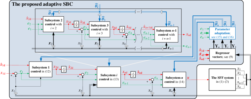
Figure 1: Diagram of the proposed adaptive SBC (highlighted in light blue). The desired variables (and the control output $u$) are shown in red, the feedback signals are in green, the adaptive control is in blue, and the system output states are in black. The bold lines are vectors and the thin lines are scalar variables.

Remark III.2

As Fig. 1 and (18)–(20) show, $\widehat{\boldsymbol{\theta}}_{k}$ in SS_k should be continuously differentiable in $C^{n-k}$ when stepping through the remaining SSs. The projection function $\mathcal{P}_{k}$ in (11) satisfies $\widehat{\boldsymbol{\theta}}_{k}\in C^{n-k}$, $\forall k\in\{1,...,n\}$. If SS_k satisfies $n-k\leqslant 1$, a projection function $\mathcal{P}\in C^{1}$ in [3, 17] can be used instead of $\mathcal{P}_{k}$. If SS_k satisfies $n-k\leqslant 2$, $\mathcal{P}_{2}\in C^{2}$ in [3, 17] can be used.

Remark III.3

As in Remark III.1, SS_k control in (18)–(20) can be reproduced with a generic and modular equation

$$g_{k}(\boldsymbol{x}_{k})x_{(k+1){\rm d}}={\mathbf{Y}}_{k}\widehat{\boldsymbol{\theta}}_{k}+\delta_{k-1}g_{k-1}(\boldsymbol{x}_{k-1}){e}_{k-1}+\lambda_{k}{e}_{k}$$

$\forall k\in\{1,...,n\}$, such that $\delta_{0}g_{0}(\boldsymbol{x}_{0}){e}_{0}=0$ and $x_{(n+1){\rm d}}=u$. The modularity in the control provides that changing SS_k dynamics, or adding/removing SSs, do not alter the structure of control laws in the remaining SSs.

Remark III.4

As the main difference to [16], we design stabilizing FB term $\delta_{k-1}g_{k-1}(\boldsymbol{x}_{k-1}){e}_{k-1}$, $\forall k\in\{2,...,n\}$, in (18)–(20) to produce stability connector $s_{k-1}$ (analyzed next in Section IV), such that passivity between SSs do not need to be considered. While the results in [16] are based on Lebesque $L_{2}$/$L_{\infty}$ integrable functions, we base the results on Lyapunov functions. We also proposed novel projection function $\mathcal{P}_{k}$ in Definition III.1 to address the system parametric uncertainties.

IV Stability Analysis

Next, we provide an in-depth analysis on the adaptive SBC in Section III-C. Respective analysis can be performed for the SBC in Section III-A using $\boldsymbol{\theta}_{k}-{\boldsymbol{\theta}}_{k}=0$ instead of $\boldsymbol{\theta}_{k}-\widehat{\boldsymbol{\theta}}_{k}$.

Motivated by a key concept in virtual stability analysis—a virtual power flow [3, Sect. 2.9.2]—we introduce a related notion of a stability connector as follows:

Definition IV.1

For the system (1)–(3) with the control (18)–(20), the stability connector $s_{k}$ is defined as

$$s_{k}=\Delta_{k}g_{k}(t,\boldsymbol{x}_{k}){e}_{k}{e}_{k+1}$$

where SS-related term $\Delta_{k}=1$, if $k=1$, and $\Delta_{k}=\frac{1}{\delta_{1}\cdots\delta_{k-1}}$, if $k>1$, and $\delta_{1},\delta_{2},\cdots,\delta_{k-1}>0$ are feedback gains from Section III.

Next, in Lemmas IV.1–IV.3 we provide auxiliary results for the convergence analysis in Theorem IV.1. Motivated by the concept of virtual stability [3, Sect. 2.9], the auxiliary analysis is carried out for the individual subsystem error dynamics $e_{k}$ and the corresponding parameter estimation errors $\boldsymbol{\theta}_{k}-\widehat{\boldsymbol{\theta}}_{k}$.

Subtracting (1) from (18), adding $\theta_{11}\dot{x}_{\rm 1d}-\theta_{11}\dot{x}_{\rm 1d}$ = 0, using (4), (9) and (10), and rearranging the terms, we get the following error dynamics for SS₁

$$\theta_{11}\dot{e}_{1}=-\lambda_{1}{e}_{1}+g_{1}({x}_{1})e_{\rm 2}+{\mathbf{Y}}_{1}({\boldsymbol{\theta}}_{1}-\widehat{\boldsymbol{\theta}}_{1}).$$ (23)

Lemma IV.1

Considering SS₁ error dynamics in (23), and $\boldsymbol{\theta}_{1}-\widehat{\boldsymbol{\theta}}_{1}$ governed by (10), (21) and (22), the derivative of the quadratic function

$$\nu_{1}=\frac{1}{2}\left(\theta_{11}{e}_{1}^{2}+\sum_{\zeta=1}^{j}\frac{(\theta_{1\zeta}-\widehat{\theta}_{1\zeta})^{2}}{\rho_{1\zeta}}\right)$$ (24)

along the trajectories of the error dynamics satisfies

$$\dot{\nu}_{1}\leqslant-\lambda_{1}{e}_{1}^{2}+s_{1}$$ (25)

where $s_{1}$ is the stability connector from Definition IV.1.

Proof:

See Appendix B. ∎

Remark IV.1

In Lemma IV.1, term $e_{2}$ in (23) is treated as an external input that causes $s_{1}$ to appear in (25) (see Appendix B) that will be canceled out based on the result of the next lemma. The dynamics of $e_{2}$ as well as the subsequent subsystems error dynamics are accounted for in the next two lemmas.

Subtracting (2) from (19), adding $\theta_{i1}\dot{x}_{i{\rm d}}-\theta_{i1}\dot{x}_{i{\rm d}}$ = 0 using (4), (9) and (10), and rearranging the terms, we get the following error dynamics for SS_i, $\forall i\in\{2,...,n-1\}$,

$$\theta_{i1}\dot{e}_{i} =-\lambda_{i}{e}_{i}-\delta_{i-1}g_{i-1}(\boldsymbol{x}_{i-1}){e}_{i-1}+g_{i}(\boldsymbol{x}_{i})e_{i+1}$$

$$\hskip 11.38092pt+{\mathbf{Y}}_{i}({\boldsymbol{\theta}}_{i}-\widehat{\boldsymbol{\theta}}_{i}).$$ (26)

Lemma IV.2

Considering SS_i error dynamics in (26), and $\boldsymbol{\theta}_{i}-\widehat{\boldsymbol{\theta}}_{i}$ governed by (10), (21) and (22), the derivative of the quadratic function

$$\nu_{i}=\frac{1}{2(\delta_{1}\cdots\delta_{i-1})}\left(\theta_{i1}{e}_{i}^{2}+\sum_{\zeta=1}^{j}\frac{(\theta_{i\zeta}-\widehat{\theta}_{i\zeta})^{2}}{\rho_{i\zeta}}\right)$$ (27)

along the trajectories of the error dynamics satisfies

$$\dot{\nu}_{i}\leqslant-\frac{\lambda_{i}}{\delta_{1}\cdots\delta_{i-1}}{e}_{i}^{2}-s_{i-1}+s_{i}$$ (28)

where $s_{i-1}$ and $s_{i}$ are the stability connectors from Definition IV.1.

Proof:

See Appendix B. ∎

Remark IV.2

Similarly to Lemma IV.1, $e_{i+1}$ in (26) is treated as an external input that causes $s_{i}$ to appear in (28). The stabilizing FB term $\delta_{i-1}g_{i-1}(\boldsymbol{x}_{i-1}){e}_{i-1}$ in (26) creates another stability connector $-s_{i-1}$ to appear in (28) (see Appendix B) that will cancel out $s_{i-1}$ from the previous SS. The last connector $s_{n-1}$ will be canceled out based on the result of the next lemma, after which we are in the position to present the convergence result for the overall error dynamics.

Subtracting (3) from (20), adding $\theta_{n1}\dot{x}_{n{\rm d}}-\theta_{n1}\dot{x}_{n{\rm d}}$ = 0 using (4), (9) and (10), and rearranging the terms, we get the following error dynamics for SS_n

$$\theta_{n1}\dot{e}_{n}=-\lambda_{n}{e}_{n}-\delta_{n-1}g_{n-1}(\boldsymbol{x}_{n-1}){e}_{n-1}+{\mathbf{Y}}_{n}({\boldsymbol{\theta}}_{n}-\widehat{\boldsymbol{\theta}}_{n}).$$ (29)

Lemma IV.3

Considering SS_n error dynamics in (29), and $\boldsymbol{\theta}_{n}-\widehat{\boldsymbol{\theta}}_{n}$ governed by (10), (21) and (22), the derivative of the quadratic function

$$\nu_{n}=\frac{1}{2(\delta_{1}\cdots\delta_{n-1})}\left(\theta_{n1}{e}_{n}^{2}+\sum_{\zeta=1}^{j}\frac{(\theta_{n\zeta}-\widehat{\theta}_{n\zeta})^{2}}{\rho_{n\zeta}}\right)$$ (30)

along the trajectories of the error dynamics satisfies

$$\dot{\nu}_{n}\leqslant-\frac{\lambda_{n}}{\delta_{1}\cdots\delta_{n-1}}{e}_{n}^{2}-s_{n-1}$$ (31)

where $s_{n-1}$ is the stability connector from Definition IV.1.

Proof:

See Appendix B. ∎

We will now construct a Lyapunov candidate for the overall error dynamics as the sum of the quadratic functions from Lemmas IV.1–IV.3. Based on the properties derived in the lemmas, we obtain that the error dynamics will remain bounded, and moreover, that the control errors converge globally asymptotically to zero. The result is given in the following theorem.

Theorem IV.1

Consider the error dynamics $\boldsymbol{e}=[e_{1},\ldots,e_{n}]^{T}$ and the parameter estimation error $\boldsymbol{\theta}_{k}-\widehat{\boldsymbol{\theta}}_{k}$, $\forall k\in\{1,2,\ldots,n\}$, that are governed in Lemmas IV.1–IV.3. For arbitrary initial conditions, $\boldsymbol{\theta}_{k}-\widehat{\boldsymbol{\theta}}_{k}$ remains bounded and $e_{k}(t)\to 0$ globally as $t\to\infty$ for all $k\in\{1,2,\ldots,n\}$.

Proof:

Using (24), (27) and (30), we choose a Lyapunov candidate function for the overall error dynamics as

$$\nu_{\rm tot} =\nu_{1}+\sum_{i=2}^{n-1}{\nu_{i}}+\nu_{n}$$

$$=\frac{1}{2}\boldsymbol{e}^{T}{\mathbf{A}}\boldsymbol{e}+\sum_{k=1}^{n}\frac{1}{2(\delta_{1}\cdots\delta_{k-1})}\sum_{\zeta=1}^{j}\frac{(\theta_{k\zeta}-\widehat{\theta}_{k\zeta})^{2}}{\rho_{k\zeta}}$$

where ${\mathbf{A}}={diag}\left(\theta_{11},\frac{\theta_{21}}{\delta_{1}},\frac{\theta_{31}}{\delta_{1}\delta_{2}},\cdots,\frac{\theta_{n1}}{\delta_{1}\cdots\delta_{n-1}}\right)\in\mathbb{R}^{n\times n}$ is positive definite. Then, it follows from (25), (28) and (31) that

$$\hskip 85.35826pt\dot{\nu}_{\rm tot}=\dot{\nu}_{1}+\sum_{i=2}^{n-1}\dot{\nu}_{i}+\dot{\nu}_{n}$$

$$\hskip 102.43008pt\leqslant-\lambda_{1}{e}_{1}^{2}+s_{1}-\sum_{i=2}^{n-1}\left[\frac{\lambda_{i}}{\delta_{1}\cdots\delta_{i-1}}{e}_{i}^{2}-s_{i-1}+s_{i}\right]-\frac{\lambda_{n}}{\delta_{1}\cdots\delta_{n-1}}{e}_{n}^{2}-s_{n-1}$$

$$\hskip 102.43008pt=-\lambda_{1}{e}_{1}^{2}-\sum_{i=2}^{n-1}\frac{\lambda_{1}}{\delta_{1}\cdots\delta_{i-1}}{e}_{i}^{2}-\frac{\lambda_{n}}{\delta_{1}\cdots\delta_{n-1}}{e}_{n}^{2}+\sum_{k=1}^{n-1}(s_{k}-s_{k})$$

$$\hskip 102.43008pt=-\boldsymbol{e}^{T}{\mathbf{B}}\boldsymbol{e}$$

where ${\mathbf{B}}={diag}\left(\lambda_{1},\frac{\lambda_{2}}{\delta_{1}},\frac{\lambda_{3}}{\delta_{1}\delta_{2}},\cdots,\frac{\lambda_{n}}{\delta_{1}\cdots\delta_{n-1}}\right)\in\mathbb{R}^{n\times n}$ is positive definite and every stability connector $s_{k}$ is canceled by its negative counterpart $-s_{k}$, $\forall k\in\{1,2,...,n-1\}$. By [18, Thm. 8.4] both the control errors and the parameter estimation errors are bounded, and $\boldsymbol{e}(t)^{T}{\mathbf{B}}\boldsymbol{e}(t)\to 0$ globally as $t\to\infty$, which by the positive-definiteness of $\mathbf{B}$ is equivalent to $\boldsymbol{e}(t)\to\bf 0$ as $t\to\infty$, i.e., $e_{k}(t)\to 0$, $\forall k\in\{1,2,\ldots,n\}$ as $t\to\infty$. ∎

Finally, motivated by the original concept of virtual stability [3, Sect. 2.9], Definition IV.2 generalizes the results in Lemmas IV.1–IV.3 for virtual stability of the kth subsystem.

Definition IV.2

The kth subsystem, $\forall k\in\{1,...,n\}$, in (1)–(3), combined with its respective control in (18)–(22), is said to be virtually stable if the derivative of a quadratic function $\nu_{k}=\alpha_{k}{e}_{k}^{2}+(\boldsymbol{\theta}_{k}-\widehat{\boldsymbol{\theta}}_{k})^{T}{\boldsymbol{\Gamma}}_{k}(\boldsymbol{\theta}_{k}-\widehat{\boldsymbol{\theta}}_{k})$ along the trajectories of the error dynamics satisfies $\dot{\nu}_{k}\leqslant-\beta_{k}{e}_{k}^{2}-s_{k-1}+s_{k}$ for some $\alpha_{k},\beta_{k}>0$ and positive-definite ${\boldsymbol{\Gamma}}_{k}\in\mathbb{R}^{k\times k}$, where $s_{k-1}$ and $s_{k}$ are the stability connectors by Def. IV.1 such that $s_{0}=0$ and $s_{n}=0$.

Remark IV.3

Definition IV.2 provides generic tools to design local subsystem-based control for SFF systems. As we demonstrated in Theorem IV.1, virtual stability of every SS in the sense of Definition IV.2 (derived from Lemmas IV.1–IV.3) guarantees global asymptotic stability of the overall system.

V Numerical Validation

In order to validate the proposed method, we consider the 3rd order nonlinear system from [8, 9], namely,

$$\dot{x}_{1} =a_{1}x_{1}^{3}+x_{2}$$

$$\dot{x}_{2} =a_{2}(x_{1}^{2}+x_{2}^{2})+x_{3}$$ (32)

$$\dot{x}_{3} =u.$$

Using (18)–(20), the proposed adaptive SBC for the system in (32) can be designed as

$$x_{\rm 2d} ={\mathbf{Y}}_{1}\widehat{\boldsymbol{\theta}}_{1}+\lambda_{1}{e}_{1}$$

$$x_{\rm 3d} ={\mathbf{Y}}_{2}\widehat{\boldsymbol{\theta}}_{2}+\lambda_{2}{e}_{2}+\delta_{1}{e}_{1}$$ (33)

$$u ={\rm Y}_{3}\widehat{\theta}_{3}+\lambda_{3}{e}_{3}+\delta_{2}{e}_{2}$$

where ${\mathbf{Y}}_{1}=[\dot{x}_{\rm 1d}\ \ -x_{1}^{3}]$, ${\boldsymbol{\theta}}_{1}=[1\ \ \theta_{12}]^{T}$, ${\mathbf{Y}}_{2}=[\dot{x}_{\rm 2d}$ $-(x_{1}^{2}+x_{2}^{2})]$, ${\boldsymbol{\theta}}_{2}=[1\ \ \theta_{22}]^{T}$, ${\rm Y}_{3}=\dot{x}_{\rm 3d}$ and ${\theta}_{3}=$ ${\theta}_{31}=1$. The parameters in $\widehat{\boldsymbol{\theta}}_{k}$, $\forall k\in\{1,2,3\}$, are updated with $\mathcal{P}_{k}$ in Definition III.1. For simplicity, only parameters $\theta_{12}$ and $\theta_{22}$ (corresponding ${a}_{1}$ and ${a}_{2}$ in the plant) are adapted in the experiments, although possibility to adapt $\theta_{k1}$ = 1, $\forall k\in\{1,2,3\}$, remains.

To study the global asymptotic convergence suggested by Theorem IV.1, the following piecewise differentiable and sufficiently smooth reference trajectory $x_{\rm 1d}(t)$ is used

$$x_{\rm 1d}(t)=\left\{\begin{array}[]{l}{\rm sin}(2\pi t){\rm tanh}(t^{3}),\hskip 5.69046pt{\rm if}\ 0\leqslant t\leqslant 5\\ {\rm sin}(2\pi t){\rm tanh}(t^{3})[1-{\rm tanh}((t-5)^{3})],\hskip 5.69046pt{\rm if}\ t>5.\end{array}\right.$$ (36)

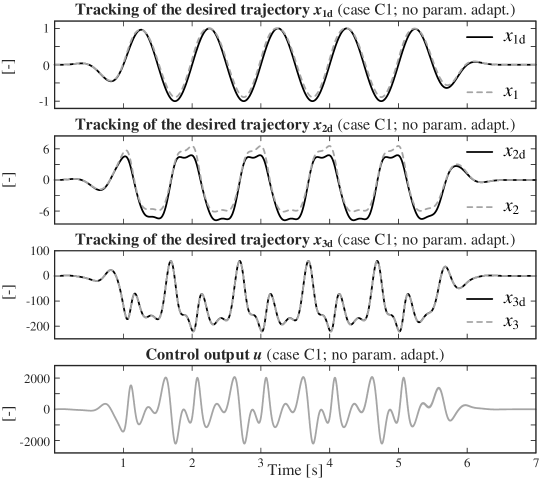
Figure 2: Control performance in C1 with inaccurate parameter values $\theta_{12}$ = 6 and $\theta_{22}$ = 4 in relation to the actual plant parameters $a_{1}$ = 5 and $a_{2}$ = 5. The desired trajectories are shown in black and their controlled variables in gray (plots 1–3). The last plot shows the control output $u$.

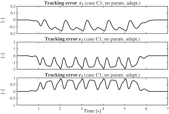
Figure 3: Tracking errors $e_{k}$, $\forall k\in\{1,2,3\}$, in C1 (adaptive control disabled).

Throughout the simulations, $a_{1}$ = 5 and $a_{2}$ = 5 are used for the plant in (32), and the FB gains were loosely tuned to $\lambda_{1}$ = 10, $\lambda_{2}$ = 20, $\lambda_{3}$ = 40, $\delta_{1}$ = 10 and $\delta_{2}$ = 20. The sample time in simulations was set to 0.01 ms to address the exponential rate of dynamics. The following three test cases are studied:

C1:

The baseline SBC (in Sec. III-A) is employed, i.e., ${\boldsymbol{\theta}}_{1}$, ${\boldsymbol{\theta}}_{2}$ and ${\theta}_{3}$ (instead of $\widehat{\boldsymbol{\theta}}_{1}$, $\widehat{\boldsymbol{\theta}}_{2}$ and $\widehat{\theta}_{3}$) are used in (33). In addition, inaccurate FF parameters $\theta_{12}$ = 6 and $\theta_{22}$ = 4 are used in relation to their respective plant parameters $a_{1}=5$ and $a_{2}=5$ in (32). Figs. 2 and 3 show the results.

C2:

The proposed adaptive SBC (in Sec. III-C) is employed with initial parameter estimate values $\widehat{\theta}_{12}(0)$ = 6 and $\widehat{\theta}_{22}$(0) = 4 in (33). Figs. 4–6 show the results.

C3:

The proposed adaptive SBC (in Sec. III-C) is employed with initial parameter estimate values $\widehat{\theta}_{12}(0)$ = 0.1 and $\widehat{\theta}_{22}$(0) = 9.9. Figs. 5 and 6 show the results.

In cases C2 and C3 with the adaptive control, the parameter update gains were set to $\rho_{12}=1000$, $\sigma_{12}=1000/\rho_{12}$, $\rho_{22}=2$ and $\sigma_{22}=1000/\rho_{22}$; the parameter bounds were set to $\overline{\theta}_{12}=9$, $\underline{\theta}_{12}=1$, $\overline{\theta}_{22}=9$ and $\underline{\theta}_{22}=1$; and the activation intervals beyond the bounds were set to 0.5 ($c_{\rm 21}=0.5$ and $c_{\rm 22}=0.5$)

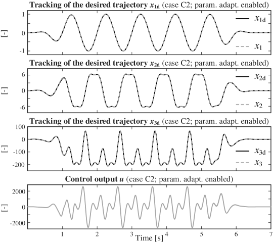
Figure 4: Control performance in C2 with initial parameter values $\widehat{\theta}_{12}(0)$ = 6 and $\widehat{\theta}_{22}(0)$ = 4, while $a_{1}$ = 5 and $a_{2}$ = 5 hold for the respective plant parameters. The desired trajectories are shown in black and their controlled variables in gray (plots 1–3). The last plot shows the control output $u$.

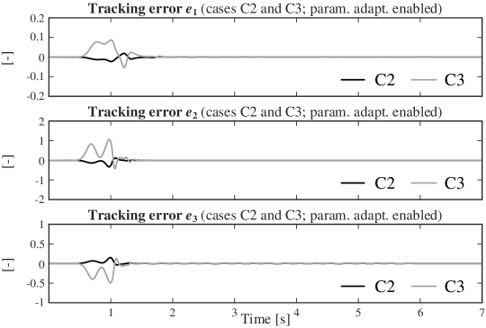
Figure 5: Tracking errors $e_{k}$, $\forall k\in\{1,2,3\}$, in C2 and C3 (adaptive control enabled). The results in C2 are in black and the results in C3 are in gray.

Figs. 2 and 3 show the results in case C1, where the control for the plant is designed by the theory in Section III-A. However, inaccurate FF parameters (i.e., $\theta_{12}\neq a_{1}$ and $\theta_{22}\neq a_{2}$) are used such that, in cases C2 and C3, comparisons can be made to the proposed adaptive SBC. In plots 1–3, Fig. 2 shows the desired trajectory $x_{k{\rm d}}$, $\forall k\in\{1,2,3\}$, in black and its controlled state $x_{k}$ in gray. The last plot shows the control output $u$. The detailed tracking errors are shown in Fig. 3, the maximum absolute tracking errors being $|e_{1}|_{\rm max}$ = 0.163, $|e_{2}|_{\rm max}$ = 1.877 and $|e_{3}|_{\rm max}$ = 0.924. As can be seen, noticeable tracking errors occur in the transition phases due to the parametric uncertainty.

Figs. 4–6 show the main results of the study with the proposed adaptive SBC in (33). Fig. 4 shows the tracking results in case C2 where the initial values for the parameter estimates are selected in accordance to case C1, i.e., $\widehat{\theta}_{12}(0)$ = 6 and $\widehat{\theta}_{22}(0)$ = 4. As the black lines in Fig. 5 shows, the tracking errors are substantially decreased in relation to case C1, with the maximum absolute tracking errors $|e_{1}|_{\rm max}$ = 0.023, $|e_{2}|_{\rm max}$ = 0.336 and $|e_{3}|_{\rm max}$ = 0.152. As predicted by the theory, global asymptotic convergence is achieved. Fig. 6 shows the behavior of the parameter estimates $\widehat{\theta}_{12}$ and $\widehat{\theta}_{22}$ in black, illustrating that the proposed projection function ${\mathcal{P}}_{k}$ actively pushes the parameter values toward their real values in the plant.

In the last case C3, the initial parameter values are set outside the projection function ${\mathcal{P}}_{k}$ bounds such that $\widehat{\theta}_{12}$(0) = 0.1 and $\widehat{\theta}_{22}$(0) = 9.9. The results are shown in Figs. 5 and 6 in gray. Despite a significant inaccuracy in the initial parameter values, the projection function ${\mathcal{P}}_{k}$ actively pushes the parameter values toward their real values in the plant (see Fig. 6), with the maximum absolute tracking errors $|e_{1}|_{\rm max}$ = 0.087, $|e_{2}|_{\rm max}$ = 1.060 and $|e_{3}|_{\rm max}$ = 0.496 (see Fig. 5). After 1.5 s the control behavior in case C3 becomes virtually identical to case C2.

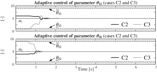
Figure 6: Adapted parameters $\widehat{\theta}_{12}(t)$ (the 1st plot) and $\widehat{\theta}_{22}(t)$ (the 2nd plot). The results in C2 ($\widehat{\theta}_{12}(0)$ = 6 and $\widehat{\theta}_{22}(0)$ = 4) are given in black, while the result in C3 ($\widehat{\theta}_{12}(0)$ = 0.1 and $\widehat{\theta}_{22}(0)$ = 9.9) are given in dark gray. The plant parameters $a_{1}$ = 5 and $a_{2}$ = 5 are shown in dashed line. The upper bound $\overline{\theta}$ = 9 and lower bound $\underline{\theta}$ = 1 are shown in dashed-dot line. The bound activation intervals (defined by $c_{\rm 21}=0.5$ and $c_{\rm 22}=0.5$) are in gray.

VI Conclusions

This study proposed an adaptive subsystem-based control for controlling nth-order SFF systems with parametric uncertainties. As an alternative for backstepping, we provided systematic and straightforward tools for globally asymptotically stable control while avoiding a growth of the control design complexity when the system order n increases. The proposed method is modular in the sense that the control for every SS can be designed with a single generic-form equation such that changing SS dynamics or removing/adding SSs do not affect to the control laws in the remaining SSs. For the method, we reformulated the original concept of virtual stability in [3, Def. 2.17] and proposed a specific stability connector to address dynamic interactions between the adjacent SSs. These features enable that both the control design and the stability analysis can be performed locally at a SS level (as opposed to the whole system); see Remark IV.3. We proposed also a smooth projection function ${\mathcal{P}}_{k}$ for the system parametric uncertainties. Theoretical developments on global asymptotic convergence (in Theorem IV.1) were verified in numerical simulations. Semi-SFF systems with unknown dynamics remain a subject for future studies.

Appendix A The Projection Function $\mathcal{P}_{k}$

Consider the piecewise-continuous projection function $\mathcal{P}_{k}$ in Definition III.1. Parameters $a$ and $b$ define the lower and upper bounds for $\mathcal{P}_{k}$ such that $b\geqslant a>0$. Within the bounds, $\dot{\mathcal{P}}_{k}$ is driven by $\rho{\rm p}(t)$ and the behavior of $\mathcal{P}_{k}$ is equal to $\mathcal{P}\in C^{1}$ and $\mathcal{P}_{2}\in C^{2}$ in [3, 17]. Outside the bounds, a corrective term $\sigma{\kappa}$ is designed to bring $\mathcal{P}_{k}$ back toward the bounds. The parameter $c$ defines activation interval lengths $(a-c,a)$ and $(b,b+c)$ for the switching functions $S_{a}(\mathcal{P}_{k})$ and $S_{b}(\mathcal{P}_{k})$.

Let $|{\rm p}^{(n-k)}(t)|<+\infty$, $\forall k\in\{1,...,n\}$. To guarantee the existence of ${\mathcal{P}^{(k)}_{k}}$ outside the bounds, the switching functions $S_{a}(\mathcal{P}_{k}):(a-c,a)\to(1,0)$ and $S_{b}(\mathcal{P}_{k}):(b,b+c)\to(0,1)$ are required to satisfy the boundary conditions [in (LABEL:EQ_BCa) and (LABEL:EQ_BCb)]

$${\lim_{x\to(a-c)^{+}}}S_{a}(x)=1,\hskip 5.69046pt{\lim_{x\to(a-c)^{+}}}S_{a}^{(j)}(x)=0,$$ (37)

$$\hskip 7.11317pt{\lim_{x\to a^{-}}}S_{a}(x)=0\ \ {\rm and}\ {\lim_{x\to a^{-}}}S_{a}^{(j)}(x)=0,$$

$${\lim_{x\to(b+c)^{-}}}S_{b}(x)=1,\hskip 5.69046pt{\lim_{x\to(b+c)^{-}}}S_{b}^{(j)}(x)=0,$$ (38)

$$\hskip 7.11317pt{\lim_{x\to b^{+}}}S_{b}(x)=0\ \ {\rm and}\ {\lim_{x\to b^{+}}}S_{b}^{(j)}(x)=0,$$

$\forall j\in\{1,...,n-1\}$. Definition A.1 provides smooth and strictly decreasing solution for $S_{a}(\mathcal{P}_{k})$, satisfying (LABEL:EQ_BCa), and smooth and strictly increasing solution for $S_{b}(\mathcal{P}_{k})$, satisfying (LABEL:EQ_BCb).

Definition A.1

$S_{a}(\mathcal{P}_{k}):(a-c,a)\to(1,0)$ is a smooth and strictly decreasing switching function defined as

$$S_{a}(\mathcal{P}_{k}):=\frac{1}{2}\left[1-\tanh\left(\frac{1}{a-c-\mathcal{P}_{k}}+\frac{1}{a-\mathcal{P}_{k}}\right)\right]$$

and $S_{b}(\mathcal{P}_{k}):(b,b+c)\to(0,1)$ is a smooth and strictly increasing switching function defined as

$$S_{b}(\mathcal{P}_{k}):=\frac{1}{2}\left[1+\tanh\left(\frac{1}{b-\mathcal{P}_{k}}+\frac{1}{b+c-\mathcal{P}_{k}}\right)\right].$$

The projection function in (11) has the following property.

Lemma A.1

For any constant $\mathcal{P}_{c}$ with $a\leqslant\mathcal{P}_{c}\leqslant b$ we have

$$({\mathcal{P}_{c}}-\mathcal{P}_{k})\left({\rm p}(t)-\frac{1}{\rho}\dot{\mathcal{P}}_{k}\right)\leqslant-\sigma\kappa^{2}\leqslant 0.$$ (39)

Proof:

The proof of Lemma A.1 follows a similar procedure as the proof of Lemma 2.10 in [3]. Let $a\leqslant{\mathcal{P}_{c}}\leqslant b$. Then, for a constant ${\mathcal{P}_{c}}$ we have

$$({\mathcal{P}_{c}}-\mathcal{P}_{k}) \geqslant(a-\mathcal{P}_{k})$$ (40)

$$(\mathcal{P}_{k}-{\mathcal{P}_{c}}) \geqslant(\mathcal{P}_{k}-b).$$ (41)

Substituting (11) into (39) we get

$$({\mathcal{P}_{c}}-\mathcal{P}_{k})\left({\rm p}(t)-\frac{1}{\rho}\dot{\mathcal{P}}_{k}\right)=-\sigma({\mathcal{P}_{c}}-\mathcal{P}_{k}){\kappa}.$$ (42)

When $\mathcal{P}_{n}\leqslant a-c$, Definition III.1 yields ${\kappa}=(a-\mathcal{P}_{k})$. Using (40), we get

$$-\sigma({\mathcal{P}_{c}}-\mathcal{P}_{k}){\kappa}\leqslant-\sigma(a-\mathcal{P}_{k}){\kappa}=-\sigma\kappa^{2}\leqslant 0.$$ (43)

When $a-c<\mathcal{P}_{k}<a$, Definition III.1 yields ${\kappa}=(a-\mathcal{P}_{k})S_{a}(\mathcal{P}_{k})$ and $S_{a}(\mathcal{P}_{k})\in(0,1)$. Using (40), we get

$$-\sigma({\mathcal{P}_{c}}-\mathcal{P}_{k}){\kappa} \leqslant-\sigma(a-\mathcal{P}_{k}){\kappa}$$

$$<-\sigma(a-\mathcal{P}_{k})S_{a}(\mathcal{P}_{k}){\kappa}$$

$$=-\sigma\kappa^{2}\leqslant 0.$$ (44)

When $a\leqslant\mathcal{P}_{k}\leqslant b$, Definition III.1 yields ${\kappa}=0$ and we get

$$-\sigma({\mathcal{P}_{c}}-\mathcal{P}_{k}){\kappa}=0.$$ (45)

When $b<\mathcal{P}_{k}<b+c$, Definition III.1 yields ${\kappa}=(b-\mathcal{P}_{k})S_{b}(\mathcal{P}_{k})$ and $S_{b}(\mathcal{P}_{k})\in(0,1)$. Using (41), we get

$$-\sigma({\mathcal{P}_{c}}-\mathcal{P}_{k}){\kappa} =\sigma(\mathcal{P}_{k}-{\mathcal{P}_{c}}){\kappa}$$

$$\leqslant\sigma(\mathcal{P}_{k}-b){\kappa}$$

$$<\sigma(\mathcal{P}_{k}-b)S_{b}(\mathcal{P}_{k}){\kappa}$$

$$=-\sigma(b-\mathcal{P}_{k})S_{b}(\mathcal{P}_{k}){\kappa}$$

$$=-\sigma\kappa^{2}\leqslant 0.$$ (46)

When $\mathcal{P}_{k}\geqslant b+c$, Definition III.1 yields ${\kappa}=(b-\mathcal{P}_{k})$. Using (41), we get

$$-\sigma({\mathcal{P}_{c}}-\mathcal{P}_{k}){\kappa} =\sigma(\mathcal{P}_{k}-{\mathcal{P}_{c}}){\kappa}$$

$$\leqslant\sigma(\mathcal{P}_{k}-b){\kappa}$$

$$=-\sigma(b-\mathcal{P}_{k}){\kappa}$$

$$=-\sigma\kappa^{2}\leqslant 0.$$ (47)

Finally, (43)–(A) together with (42) complete the proof. ∎

Appendix B Proofs of Lemmas IV.1, IV.2, and IV.3

Proof of Lemma IV.1: Using (23), Definition IV.1 and Lemma A.1, the derivative of the quadratic function $\nu_{1}$ in (24) can be written as

$$\dot{\nu}_{1} ={e}_{1}\theta_{11}\dot{e}_{1}-\sum_{\zeta=1}^{j}(\theta_{1\zeta}-\widehat{\theta}_{1\zeta})\frac{\dot{\widehat{\theta}}_{1\zeta}}{\rho_{1\zeta}}$$

$$=-\lambda_{1}{e}_{1}^{2}+g_{1}({x}_{1}){e}_{1}{e}_{2}+{e}_{1}{\mathbf{Y}}_{1}({\boldsymbol{\theta}}_{1}-\widehat{\boldsymbol{\theta}}_{1})-\sum_{\zeta=1}^{j}(\theta_{1\zeta}-\widehat{\theta}_{1\zeta})\frac{\dot{\widehat{\theta}}_{1\zeta}}{\rho_{1\zeta}}$$

$$=-\lambda_{1}{e}_{1}^{2}+g_{1}({x}_{1}){e}_{1}{e}_{2}+\sum_{\zeta=1}^{j}({\theta}_{1\zeta}-\widehat{{\theta}}_{1\zeta})\left({\rm p}_{1\zeta}-\frac{\dot{\widehat{{\theta}}}_{1\zeta}}{{\rho}_{1\zeta}}\right)$$

$$\leqslant-\lambda_{1}{e}_{1}^{2}+s_{1}$$

which completes the proof of Lemma IV.1. $\blacksquare$

Proof of Lemma IV.2: Using (26), Definition IV.1 and Lemma A.1, the derivative of the quadratic function $\nu_{i}$ in (27), $\forall i\in\{2,...,$ $n-1\}$, can be written as

$$\hskip 93.89418pt\dot{\nu}_{i}={e}_{i}\frac{\theta_{i1}}{\delta_{1}\cdots\delta_{i-1}}\dot{e}_{i}-\frac{1}{\delta_{1}\cdots\delta_{i-1}}\sum_{\zeta=1}^{j}(\theta_{i\zeta}-\widehat{\theta}_{i\zeta})\frac{\dot{\widehat{\theta}}_{i\zeta}}{\rho_{i\zeta}}$$

$$\hskip 102.43008pt={e}_{i}\frac{1}{\delta_{1}\cdots\delta_{i-1}}\Big{[}g_{i}(\boldsymbol{x}_{i})e_{i+1}-\delta_{i-1}g_{i-1}(\boldsymbol{x}_{i-1}){e}_{i-1}-\lambda_{i}{e}_{i}+{\mathbf{Y}}_{i}({\boldsymbol{\theta}}_{i}-\widehat{\boldsymbol{\theta}}_{i})\Big{]}$$

$$\hskip 113.81102pt-\frac{1}{\delta_{1}\cdots\delta_{i-1}}\sum_{\zeta=1}^{j}(\theta_{i\zeta}-\widehat{\theta}_{i\zeta})\frac{\dot{\widehat{\theta}}_{i\zeta}}{\rho_{i\zeta}}$$

$$\hskip 102.43008pt=-\frac{\lambda_{i}}{\delta_{1}\cdots\delta_{i-1}}{e}_{i}^{2}-\frac{1}{\delta_{1}\cdots\delta_{i-2}}g_{i-1}(\boldsymbol{x}_{i-1}){e}_{i-1}{e}_{i}+\frac{1}{\delta_{1}\cdots\delta_{i-1}}g_{i}(\boldsymbol{x}_{i}){e}_{i}{e}_{i+1}$$

$$\hskip 113.81102pt+\frac{1}{\delta_{1}\cdots\delta_{i-1}}\sum_{\zeta=1}^{j}({\theta}_{i\zeta}-\widehat{{\theta}}_{i\zeta})\left({\rm p}_{i\zeta}-\frac{\dot{\widehat{{\theta}}}_{i\zeta}}{{\rho}_{i\zeta}}\right)$$

$$\hskip 102.43008pt\leqslant-\frac{\lambda_{i}}{\delta_{1}\cdots\delta_{i-1}}{e}_{i}^{2}-s_{i-1}+s_{i}$$

which completes the proof of Lemma IV.2. $\blacksquare$

Proof of Lemma IV.3: Using (29), Definition IV.1 and Lemma A.1, the derivative of the quadratic function $\nu_{n}$ in (30) can be written as

$$\dot{\nu}_{n} ={e}_{n}\frac{\theta_{n1}}{\delta_{1}\cdots\delta_{n-1}}\dot{e}_{n}-\frac{1}{\delta_{1}\cdots\delta_{n-1}}\sum_{\zeta=1}^{j}(\theta_{n\zeta}-\widehat{\theta}_{n\zeta})\frac{\dot{\widehat{\theta}}_{n\zeta}}{\rho_{n\zeta}}$$

$$={e}_{n}\frac{1}{\delta_{1}\cdots\delta_{n-1}}\Big{[}-\lambda_{n}{e}_{n}-\delta_{n-1}g_{n-1}(\boldsymbol{x}_{n-1}){e}_{n-1}+{\mathbf{Y}}_{n}({\boldsymbol{\theta}}_{n}-\widehat{\boldsymbol{\theta}}_{n})\Big{]}-\frac{1}{\delta_{1}\cdots\delta_{n-1}}\sum_{\zeta=1}^{j}(\theta_{n\zeta}-\widehat{\theta}_{n\zeta})\frac{\dot{\widehat{\theta}}_{n\zeta}}{\rho_{n\zeta}}$$

$$=-\frac{\lambda_{n}}{\delta_{1}\cdots\delta_{n-1}}{e}_{n}^{2}-\frac{1}{\delta_{1}\cdots\delta_{n-2}}g_{n-1}(\boldsymbol{x}_{n-1}){e}_{n-1}{e}_{n}+\frac{1}{\delta_{1}\cdots\delta_{n-1}}\sum_{\zeta=1}^{j}({\theta}_{n\zeta}-\widehat{{\theta}}_{n\zeta})\left({\rm p}_{n\zeta}-\frac{\dot{\widehat{{\theta}}}_{n\zeta}}{{\rho}_{n\zeta}}\right)$$

$$\leqslant-\frac{\lambda_{n}}{\delta_{1}\cdots\delta_{n-1}}{e}_{n}^{2}-s_{n-1}$$

which completes the proof of Lemma IV.3. $\blacksquare$

References

• [1] J.-J. E. Slotine and W. Li, Applied nonlinear control, Prentice-Hall Englewood Cliffs, NJ, 1991.
• [2] S. Skogestad and I. Postlethwaite, Multivariable feedback control: analysis and design, vol. 2, New York: Wiley, 2007.
• [3] W.-H. Zhu, Virtual Decomposition Control - Toward Hyper Degrees of Freedom Robots, Springer-Verlag, 2010.
• [4] L. Hunt, R. Su, and G. Meyer, “Global transformations of nonlinear systems,” IEEE Trans. Autom. Control, vol. 28, no. 1, pp. 24–31, 1983.
• [5] M. Krstić, I. Kanellakopoulos, and P. Kokotović, Nonlinear and Adaptive Control Design, John Wiley & Sons, Inc., 1995.
• [6] D. Swaroop, J. K. Hedrick, P. P. Yip, and J. C. Gerdes, “Dynamic surface control for a class of nonlinear systems,” IEEE Trans. Autom. Control, vol. 45, no. 10, pp. 1893–1899, 2000.
• [7] B. Song and J. K. Hedrick, Dynamic surface control of uncertain nonlinear systems: an LMI approach, Springer Science & Business Media, 2011.
• [8] P. P. Yip and J. K. Hedrick, “Adaptive dynamic surface control: a simplified algorithm for adaptive backstepping control of nonlinear systems,” Int. J. Control, vol. 71, no. 5, pp. 959–979, 1998.
• [9] D. Wang and J. Huang, “Neural network-based adaptive dynamic surface control for a class of uncertain nonlinear systems in strict-feedback form,” IEEE Trans. Neural Netw., vol. 16, no. 1, pp. 195–202, 2005.
• [10] J.-J. Slotine and J. K. Hedrick, “Robust input-output feedback linearization,” Int. J. control, vol. 57, no. 5, pp. 1133–1139, 1993.
• [11] M. Won and J. K. Hedrick, “Multiple-surface sliding control of a class of uncertain nonlinear systems,” Int. J. Control, vol. 64, no. 4, pp. 693–706, 1996.
• [12] W.-H. Zhu, Y.-G. Xi, Z.-J. Zhang, Z. Bien, and J. De Schutter, “Virtual decomposition based control for generalized high dimensional robotic systems with complicated structure,” IEEE Trans. Robot. Autom., vol. 13, no. 3, pp. 411–436, 1997.
• [13] S. Mastellone and A. van Delft, “The impact of control research on industrial innovation: What would it take to make it happen?,” Control Engineering Practice, vol. 111, pp. 104737, 2021.
• [14] J. Mattila, J. Koivumäki, D. Caldwell, and C. Semini, “A survey on control of hydraulic robotic manipulators with projection to future trends,” IEEE/ASME Trans. Mechatronics, vol. 22, no. 2, pp. 669–680, 2017.
• [15] J. Koivumäki and J. Mattila, “Adaptive and nonlinear control of discharge pressure for variable displacement axial piston pumps,” J. Dyn. Sys., Meas., Control, vol. 139, no. 10, pp. 101008, 2017.
• [16] P. Seiler and A. Alleyne, “Dissipative adaptive control for strict feedback form systems,” Eur. J. Control, vol. 8, no. 5, pp. 435–444, 2002.
• [17] W.-H. Zhu and J. De Schutter, “Adaptive control of mixed rigid/flexible joint robot manipulators based on virtual decomposition,” IEEE Trans. Robot. Autom., vol. 15, no. 2, pp. 310–317, 1999.
• [18] H.K. Khalil, Nonlinear systems, Prentice Hall, 3rd edition, 2002.