On the impact of MDP design for Reinforcement Learning agents in Resource Management

Abstract

The recent progress in Reinforcement Learning applications to Resource Management presents Markov Decision Processes without a deeper analysis of the impacts of design decisions on agent performance. In this paper, we compare and contrast four different MDP variations, discussing their computational requirements and impacts on agent performance by means of an empirical analysis. We conclude by showing that, in our experiments, when using Multi-Layer Perceptrons as approximation function, a compact state representation allows transfer of agents between environments, and that transferred agents have good performance and outperform specialized agents in 80% of the tested scenarios, even without retraining.

1 Introduction

Deep Reinforcement Learning (DRL) has the potential of finding novel solutions to complex problems, as outlined by recent progress in diverse areas such as Control of Gene Regulatory Networks [9], adaptive video acceleration [11], and management of computational resources [7].

Resource management, the process by which we map computational resources to the tasks and jobs (programs) that require them, in particular, is an area in which recent learning approaches have demonstrated superior performance over classical algorithms and optimization techniques. Still, we see that, in recent work, each approach defines their own MDP formulations, with different design decisions. Thus, the literature lacks an analysis of the impact of certain decisions on agent performance.

In this paper, we investigate what happens to agent performance as we modify an MDP, observing the impacts when we change the state representation, the transition function, and when we shape the reward signal, performing an empirical investigation using open-source software from the deep learning and Reinforcement Learning (RL) communities.

Our main contribution is the formulation and analysis of a set of MDPs derived from one in the literature [7] that allows agents to learn faster, and to perform transfer learning with various function approximation methods. We also show that doing so does not degrade performance in the task.

The rest of this paper is organized as follows: In Section 2, we describe the papers that influenced this one, together with other deep RL work for resource management. In Section 3, we describe the theoretical background with an ongoing example applied to a resource management problem. In Section 4, we describe our methods and the proposed extensions to a base MDP. In Section 5, we describe our experimental framework, along with the experiments designed to evaluate our MDPs. In Section 6 we present our concluding remarks and a brief discussion of consequences of the work described here.

2 Related Work

In recent years, interest in Deep Reinforcement Learning (RL) applied to executing the scheduling of computing jobs was probably inspired by the Deep Resource Management (DeepRM) [7] agent and environment. DeepRM presented an approach of using Policy Gradients to schedule jobs based on CPU and memory requirements. DeepRM’s approach uses images to represent jobs, and a window of jobs from which it can choose which job to schedule next. It was shown that DeepRM can learn to schedule based on different metrics. Domeniconi et al. [3] proposed CuSH, a system that built on DeepRM to schedule for CPUs and GPUs, but proposed a hierarchical agent by introducing an additional Convolutional Neural Network (cnn) that chooses which job is going to be scheduled next, and then uses a policy network to choose the scheduling policy to use with the previously selected job. It is important to highlight a major difference between DeepRM and CuSH: whereas DeepRM learns the scheduling policy itself, CuSH is essentially a classifier, which chooses between two existing policies. This means that, even without training, CuSH’s behavior is more stable than that of DeepRM, since DeepRM-style schedulers might get stuck in local minima, as reported by de Freitas Cunha and Chaimowicz [2], who investigated the behavior of DeepRM-style agents when trained with state-of-the-art RL algorithms such as Advantage Actor-Critic (A2C) and Proximal Policy Optimization (ppo), and proposed an OpenAI Gym environment for easier evaluation of RL agents for job scheduling.

Another agent that has been proposed recently, and that learns the scheduling policy itself, is RLscheduler [16]. RLscheduler is a ppo-based agent with a fully convolutional neural network for scoring jobs in a fixed window of size 128. The major innovation in RLscheduler is in the training setting, in which the authors combine synthetic workload traces with real workload traces to present the agent with ever more difficult settings, similar to learning a curriculum of tasks.

Similarly to CuSH, other agents that use a classification approach have been proposed. A recent one is the Deep Reinforcement agent for Scheduling in HPC (DRaS) [4], which classifies jobs in three categories: ready, reserved, and backfilled. After this classification step, the cluster scheduler takes the output of this classification and allocates jobs accordingly (for example, by reserving slots in the future for reserved jobs, scheduling immediately ready jobs, and finding “holes” in the schedule for backfilled jobs). DRaS uses a five-layer cnn that works in two levels, with the first level selecting jobs for immediate and reserved execution, and the second layer for backfilled execution.

None of the papers mentioned above discuss the impact of their design decisions, resorting to only comparing their results with existing algorithms. In this paper, we aim to analyze how decisions in MDP design impact DeepRM-style algorithms, and how they impact both computational performance and scheduling performance.

3 Background

In this section, we describe the background needed to understand the techniques and methodology presented in this paper. To help in understanding, we will use a resource management problem as running example throughout this section.

3.1 Batch job scheduling

The primary goal of a job scheduler is to manage the job queue and coordinate execution of jobs in High Performance Computing (HPC) clusters, while matching jobs to resources in an efficient way. In a discrete time setting, at each time step, zero or more jobs may arrive in the queue for processing, and the scheduler’s job is to allocate jobs to resources while satisfying their resource requirements. The job scheduler guarantees jobs execute when requested resources are available, and usually guarantee there won’t be oversubscription of resources. Given this primary goal, secondary goals vary between schedulers and HPC facilities, depending on whether the hosting institution prefers to satisfy the needs of individuals submitting jobs, or the whole group of users [5].

When optimization of response time is a subgoal, it is usually modeled as the minimization of the average response time, with response time used as a synonym to turnaround time: the difference between the time a job was submitted to the time it completed execution. A metric commonly used to evaluate this is the slowdown of a job, which, for job $j$ is defined as

$$\mathrm{slowdown}(j)=\frac{(t_{f}(j)-t_{s}(j))}{t_{e}(j)}=\frac{t_{w}(j)+t_{e}(j)}{t_{e}(j)}=\frac{1}{t_{e}(j)}\left(\sum_{i=1}^{t_{w}(j)}1+\sum_{i=1}^{t_{e}(j)}1\right)\text{,}$$ (1)

where $t_{s}(j)$ is the time job $j$ was submitted, $t_{e}(j)$ is the time it took to execute job $j$, and $t_{f}(j)$ is the finish time of job $j$. The equality in the middle holds because the wait time, $t_{w}$, of a job $j$ is defined as $t_{w}(j)=t_{f}(j)-(t_{e}(j)+t_{s}(j))$.

Figure 1: A possible schedule when three jobs arrive in a scheduling system at discrete time step 1 and no more jobs are submitted to the system at least until time step 7, the last one shown in the figure.

Consider the case of three batch jobs, $j_{1}=$ , $j_{2}=$ , and $j_{3}=$ , submitted to a scheduling system with two processors, and that the three jobs were submitted “between” time step 0 and 1, such that, when transitioning from the first time step to the second, now there are three jobs waiting. Also consider that, for these jobs, the generated schedule is the one displayed in Figure 1. As shown in the figure, the jobs execute for two, three and four time steps respectively, and all of them use a single processor.

The reader should observe that different schedules can yield substantially different values of (average) slowdown. For example, the schedule shown in Figure 1 has an average slowdown equal to $\nicefrac{{1}}{{3}}\sum_{i=1}^{3}\mathrm{slowdown}(j_{i})=\nicefrac{{1}}{{3}}(1+1+\nicefrac{{3}}{{2}})=\nicefrac{{7}}{{6}}$, whereas, if we swapped $j_{3}$ with $j_{1}$, and started $j_{1}$ soon after $j_{2}$ finished, the slowdown would be $\nicefrac{{1}}{{3}}(\frac{3+2}{2}+1+1)=\nicefrac{{9}}{{6}}=\nicefrac{{3}}{{2}}$, a $\approx 29\%$ increase. Therefore, a scheduler should choose job sequences wisely, otherwise its performance can be degraded.

In this paper, we will focus our discussion on what happens when an RL system tries to minimize the average slowdown, but our conclusions are general and apply to other metrics and problems as well.

3.2 Deep Reinforcement Learning and Job Scheduling

In a Reinforcement Learning (RL) problem, an agent interacts with an unknown environment in which it attempts to optimize a reward signal by sequentially observing the environment’s state and taking actions according to its perception. For each action, the agent receives a reward. Thus, in the end, we want to find the sequence of actions that maximizes the total reward, as we will detail in the next paragraphs.

RL formalizes the problem as a Markov Decision Process (MDP) represented by a tuple $\mathcal{M}=\langle\mathcal{S},\mathcal{A},\mathcal{R},\mathcal{T},\rho,\gamma\rangle$. At each discrete time step $t$ the agent is in state $S_{t}\in\mathcal{S}$. From $S_{t}$, the agent takes an action $A_{t}\in\mathcal{A}$, receives reward $R_{t+1}\in\mathcal{R}$ and ends up in state $S_{t+1}\in\mathcal{S}$. Therefore, when we assume the first time step is $0$, the interaction between agent and environment create a sequence $S_{0},A_{0},R_{1},S_{1},A_{1},R_{2},\ldots$ of states, actions and rewards. To a specific sequence $S_{0},A_{0},R_{1},S_{1},A_{1},R_{2},\ldots$ of states, actions, and rewards we give the name of trajectory, and will denote such sequences by $\tau$. The transition from state $S_{t}$ to $S_{t+1}$ follows the probability distribution defined by $\mathcal{T}:\mathcal{S}\times\mathcal{A}\rightarrow\mathcal{S}$ or, in an equivalent way, $\mathcal{T}$ gives the probabiliy of reaching any new state $s^{\prime}$ when taking action $a$ when in state $s$: $p(s^{\prime}|s,a)=p(S_{t+1}=s^{\prime}|S_{t}=s,A_{t}=a)$. $\rho$ is a distribution of initial states, and $\gamma$ is a parameter $0\leq\gamma\leq 1$, called the discount rate. The discount rate models the present value of future rewards. For example, a reward received $k$ steps in the future is worth only $\gamma^{k}$ now. This discount factor is added due to the uncertainty in receiving rewards and is useful for modeling stochastic environments. In such cases, there is no guarantee an anticipated reward will actually be received and the discount rate models this uncertainty.

To map our presentation of RL into our problem of job scheduling, we consider $\rho(\leavevmode\hbox to11.78pt{\vbox to6.38pt{\text{[drawing]}}})=1$ (the only possible initial state is the empty cluster), with the first state consisting of the empty cluster, with no jobs in the system, $S_{0}=\langle\leavevmode\hbox to11.78pt{\vbox to6.38pt{\text{[drawing]}}}\rangle$ and $A_{0}=\emptyset$, since there is no job to schedule.

Recall our discussion about classifying jobs to be processed by different policies, versus choosing the next job to enter the system. In this paper, we are modeling an MDP in which the next job is chosen by the agent, so the agent is learning a scheduling policy. In our example, one can obtain a reward function by using the sequential version of slowdown, shown in the rightmost equality of (1), such that the reward at each time step is given by the sum of the current slowdown for all jobs in the system: $\mathcal{R}=-\sum_{j\in\mathcal{J}}\nicefrac{{1}}{{t_{e}(j)}}$. When the reward function is such that it computes the online version of slowdown for all jobs in the system, if $A_{1}=\emptyset$, $R_{2}=\nicefrac{{1}}{{2}}+\nicefrac{{1}}{{3}}+\nicefrac{{1}}{{4}}$. Moreover, if jobs $j_{1}$, $j_{2}$, and $j_{3}$ are chosen in sequence, the next state, shown in Fig. 1, will be given by sequentially applying the transition function $\mathcal{T}$ as $\mathcal{T}(\leavevmode\hbox to11.78pt{\vbox to6.38pt{\text{[drawing]}}},\leavevmode\hbox to9.97pt{\vbox to6.1pt{\text{[drawing]}}})\mathcal{T}(\leavevmode\hbox to11.78pt{\vbox to6.8pt{\text{[drawing]}}},\leavevmode\hbox to14.71pt{\vbox to6.1pt{\text{[drawing]}}})\mathcal{T}(\leavevmode\hbox to11.78pt{\vbox to6.8pt{\text{[drawing]}}},\leavevmode\hbox to19.44pt{\vbox to6.1pt{\text{[drawing]}}})$. If the episode finished immediately after the state shown in Fig. 1, the trajectory $\tau_{1}$ would be given by $\tau_{1}=\langle S_{0}=\leavevmode\hbox to11.78pt{\vbox to6.38pt{\text{[drawing]}}},A_{0}=\leavevmode\hbox to9.97pt{\vbox to6.1pt{\text{[drawing]}}},R_{1}=0,S_{1}=\leavevmode\hbox to11.78pt{\vbox to6.8pt{\text{[drawing]}}},A_{1}=\leavevmode\hbox to14.71pt{\vbox to6.1pt{\text{[drawing]}}},R_{2}=0,S_{2}=\leavevmode\hbox to11.78pt{\vbox to6.8pt{\text{[drawing]}}},\ldots\rangle$.

The reward signal encodes all of the agent’s goals and purposes, and the agent’s sole objective is to find a policy $\pi_{\theta}$ parameterized by $\theta$ that maximizes the expected return

$$G(\tau)=R_{1}+\gamma R_{2}+\cdots+\gamma^{T-1}R_{T}=\sum_{t=0}^{T-1}\gamma^{t}R(S_{t},A_{t}\sim\pi_{\theta}(S_{t}))\text{,}$$ (2)

which is the sum of discounted rewards encountered by the agent. When $T$ is unbounded, $\gamma<1$. Otherwise, Equation (2) would diverge. In our example, a deterministic policy that always chose the smallest job first would yield $\pi_{\theta}(\langle\leavevmode\hbox to11.78pt{\vbox to6.38pt{\text{[drawing]}}},\leavevmode\hbox to9.97pt{\vbox to6.1pt{\text{[drawing]}}},\leavevmode\hbox to14.71pt{\vbox to6.1pt{\text{[drawing]}}},\leavevmode\hbox to19.44pt{\vbox to6.1pt{\text{[drawing]}}}\rangle)=\leavevmode\hbox to9.97pt{\vbox to6.1pt{\text{[drawing]}}}$, while a stochastic policy would assign a probability to each job, and either choose the one with highest probability or sample from the jobs according to that distribution. In practice, when neural networks are used for approximation, the last layer of the neural network is usually a softmax, so that each action gets a number that can be interpreted as a probability. As mentioned before, in the example in this section, rewards are based on the negative online slowdown and, therefore, returns will also depend on the slowdown. The policy $\pi$ is a mapping from states and actions to a probability of taking an action $A$ when in state $S$, and the parameters $\theta$ relate to the approximation method used by the policy. Popular function approximators include linear combinations of features [6] and neural networks [15, 13].

3.3 Policy gradients

In this section we present the main optimization method we use to find policies: policy gradients. As implied by the name, we compute gradients of policy approximations, and use them to find better parameters for those functions.

Formally, we generalize policies to define distributions over trajectories with

$$\phi_{\theta}(\tau)=\rho(S_{0})\prod_{t}\pi_{\theta}(A_{t}|S_{t})\underbrace{\mathcal{T}(S_{t+1}|S_{t},A_{t})}_{\text{Environment}}\text{,}$$ (3)

in which $\pi_{\theta}$ is being optimized by the agent, and $\rho$ and $\mathcal{T}$ are provided by the environment. What (3) says is that we can assign probabilities to any trajectory, since we know the distribution of initial states $\rho$, and we know that the policy will assign probabilities to actions given states, and that, when such actions are taken, the environment will sample a new state for the agent. When we do so, we can define an optimization objective to find the optimal set of parameters

$$\theta^{*}=\arg\max_{\theta}J(\theta)=\arg\max_{\theta}\int_{\tau}G(\tau)\phi_{\theta}(\tau)d\tau\text{,}$$ (4)

where $J(\theta)$ is the performance measure given by the expected return of a trajectory, which can be approximated by a Monte Carlo estimate $\widehat{J(\theta)}=\nicefrac{{1}}{{N}}\sum_{i}G(\tau_{i})\phi_{\theta}(\tau_{i})$. If we construct $\widehat{J(\theta)}$ such that it is differentiable, we can approximate $\theta^{*}$ by gradient ascent in $\theta$, such that $\theta_{j+1}\leftarrow\theta_{j}+\alpha\nabla\widehat{J(\theta)}$, with $\alpha>0$, yielding

$$\nabla_{\theta}J(\theta)\approx\frac{1}{N}\sum_{i}G(\tau_{i})\nabla_{\theta}\log\phi_{\theta}(\tau_{i});\tau_{i}\sim\pi_{\theta}\text{.}$$ (5)

By expanding (2) by one time-step, we get the update $G(\tau)=R_{1}+\gamma G(\tau_{1})$ or, more generally, $G(\tau_{t})=R_{t+1}+\gamma G(\tau_{t+1})$, where $\tau_{i}$ indicates the trajectory $\tau$ starting from offset $i$. This update is usually written as $G_{t}=R_{t+1}+\gamma v_{\pi}(S_{t+1})$, where $G_{t}$ is shorthand notation for $G(\tau_{t})$, and $v_{\pi}(S_{t+1})$ is the return when starting at state $S_{t+1}$ and following policy $\pi$ (which generated trajectory $\tau$). Another function related to $v_{\pi}(S_{t})$ is $q_{\pi}(S_{t},A_{t})$, which gives the return when starting at state $S_{t}$ and taking action $A_{t}$ then following policy $\pi$. With these two functions, we can define a third one, which gives the relative advantage of taking action $A_{t}$ when in state $S_{t}$, defined as $a_{\pi}(S_{t},A_{t})=q_{\pi}(S_{t},A_{t})-v_{\pi}(S_{t})$, and called the advantage function. As with the policy, $q_{\pi}$, $v_{\pi}$, and $a_{\pi}$ can also be approximated and, thus, learned. When such an approximation is used, the update (5) becomes

$$\nabla_{\theta}J(\theta)\approx\frac{1}{N}\sum_{i}\nabla_{\theta}\log\pi_{\theta}(A_{t}|S_{t})\hat{a}_{\pi}(S_{t},A_{t});S_{t},A_{t}\sim\pi_{\theta}\text{,}$$ (6)

where $\hat{a}_{\pi}$ is an approximation of $a_{\pi}$, and which can be further split into two estimators as $\hat{a}_{\pi}=\hat{q}_{\pi}-\hat{v}_{\pi}$, with the arguments $S_{t}$ and $A_{t}$ dropped for better readability. In this setting, the $\pi_{\theta}$ approximator is called an actor, and the $\hat{a}_{\pi}$ approximator is called a critic.

In the literature, we find techniques that regularize updates [8, 12], but as presented, equation (6) is sufficient for understanding of the techniques discussed in this paper.

4 Methodology

Although the discussion in the previous section is helpful for conceptualizing the problem we are interested in, it is not enough to help us implement a solution, since it does not specify when the agent is invoked for learning, how a state is actually represented, nor how rewards are computed for each action. In this section, we will detail our design decisions, and will elaborate on what changes are required to assess the impact of said decisions in RL performance. We begin by describing the base MDP, and then we will describe incremental changes that can be made to the environment so that it may become faster to compute, and easier to learn, leading to faster convergence.

We implemented the base MDP and each incremental change discussed in this section. Then, we evaluated all implementations, observing both convergence performance and final agent performance in the task of scheduling HPC jobs.

4.1 The base, image-like MDP

We begin by following the design of DeepRM [7], summarized here, and exemplified in Fig. 2. We start by representing states as images whose height corresponds to a look to a time horizon of $H$ time-steps “into” the future, and the width comprising: the number of processors in the system and their occupancy state, a window of configurable size $W$ (in the Figure, $W=2$) containing the first $W$ jobs in the wait queue times the number of processors in the system, and a column vector indicating jobs in a “backlog”. If there are more jobs in the system that can fit the window and the backlog, they are omitted from the state representation.

Figure 2: Dense state representation with images representing state. In the figure, there is one job in execution (with two processors for the next two time steps), three waiting jobs in total, two of them within window $W=2$, one using one CPU for at least five time steps, and another using three CPUs for four time steps. Details for the third job, in the backlog are omitted.

For the action, the agent can either choose to schedule a job from one of the $W$ slots, or it can refuse to schedule a job, totalling three possible actions in the example of Fig. 2. Regarding when actions are taken, the MDP was built in such a way that agents see every simulation time step and “intermediate” time-steps as well: when a job is scheduled, there is a state change in the MDP, with the job moving to the in-use processors, and the queue being re-organized so that all slots in window $W$ are filled.

In the base MDP, whenever a job is scheduled, the agent receives a reward of zero. In all other cases, the reward is given by the negative online slowdown (1): $\mathcal{R}=-\sum_{j\in\mathcal{J}}\frac{1}{t_{e}(j)}$. For a detailed description of the environment, we direct the reader to Mao et al. [7], who first introduced it.

4.2 Compact state representation

The first realization we had was that the state representation in the base MDP is wasteful, in the sense that one can reduce the size of the state without losing information. Particularly when working with larger clusters, or with a larger number of job slots, it may be the case that full trajectories take too much space in memory, reducing the computational performance of learning agents. Due to that, and based on a set of features found in the literature for machine learning with HPC jobs [1], we devised a set of features that can represent states in a compact way. In our new state representation, jobs in the queue are represented by the features shown in Table 1, where “work” is computed by multiplying the number of processors a job requires by the time it is expected to run, and cluster features are a pair that indicates the number of processors in use, and the number of free processors. The features related to the cluster state still use a time horizon $H$ but instead of using a matrix, we used a pair of integers representing how many processors are in use, and how many processors are free in a given time-step. As an example, assuming the job in the cluster was submitted at time 1, the job in slot 1 was submitted at time 2, and the job in slot 2 was submitted in time 3, the state shown in Fig. 2 can be fully described by the concatenation of vectors with cluster state $\langle(2,1),(2,1),(0,3),(0,3),(0,3)\rangle$, jobs in window $W$ $\langle(1,5,1,0,0,1,6,0),(2,4,3,1,5,1,4,0)\rangle$ and backlog $\langle 1\rangle$. The features in the jobs slots are presented in the same order as the ones shown in Table 1.

Table 1: Job features in a compact state representation.

Feature	Description
Submission time	Time at which the job was submitted
Requested time	Amount of time requested to execute the job
Requested processors	Number of processors requested at the submission time
Queue size	Number of jobs in the wait queue at job submission time
Queued work	Amount of work that was in the queue at job submission time
Free processors	Amount of free processors when the job was submitted
Remaining work	Amount of work remaining to be executed at job submission time
Backlog	The number of jobs waiting outside window $W$

A side-effect of using this new compact state representation is that, when $H$ and $W$ are fixed between different cluster configurations, learned features are directly transferable between clusters even when using function approximation methods that depend on a fixed number of features.

4.3 Sparse State Transitions

Another deficiency we’ve identified in the base MDP is that the agent sees all time-steps in the simulation, but this causes the agent to have to take an action even when there is no good action to take. Consider, for example, the case in which all resources are in use (there are no free resources). In cases such as this, any action the agent takes will lead to the same outcome: increasing the simulation clock, receiving negative rewards related to the slowdown of the jobs, and having no new jobs scheduled. This will be repeated for all time steps between the start of the last job that exhausted resources until the finish of the first job that frees them, causing non-negative rewards to be more sparse, making the reinforcement signal noisier and, therefore, harder to learn. The opposite is also true: if there are no jobs waiting to be scheduled, no matter what the agent chooses, the outcome will be the same: no jobs will be scheduled.

Due to that, we updated the environment to only call the agent and, therefore, to only add states, actions and rewards to a trajectory, when it was possible for the agent to take an action that could result in a job being scheduled. In short, we change the transition function $\mathcal{T}(S_{t+1}\mid S_{t},A_{t})$ so that all state transitions from $S_{t}$ to $S_{t+1}$ will always have at least one job that may be scheduled by the agent in state $S_{t+1}$. We did not change the initial state, though, so $\rho=\{\leavevmode\hbox to11.78pt{\vbox to6.38pt{\text{[drawing]}}}\}$ still holds. This essentially turns the MDP into a semi-MDP [14]. To make our formulation compatible with a semi-MDP, we extend the reward function to return zero in all intermediate states after successfully scheduling a job.

4.4 Reducing the noise of the reward signal

Based on the idea of only showing the agent what it can use to learn and act, we noticed that the reward signal could be further improved by, instead of computing the online slowdown of all jobs in the system $\mathcal{J}$, considering only the jobs that are in the waiting queue, and within the job slots window $W$: the jobs that can be directly influenced by the agent’s actions. Therefore, we defined the set $\mathcal{W}$ that contains the subset of jobs from $\mathcal{J}$ that are within the window $W$, and the reward function became $\mathcal{R}=-\sum_{j\in\mathcal{W}}\frac{1}{t_{e}(j_{i})}$ when the action taken doesn’t schedule a job, and 0 otherwise.

We evaluate the impact of the various MDPs on agent performance by performing two sets of experiments, one in which we observe the impact of the changes proposed in Sections 4.2 through 4.4 (called Compact, Sparse, and Reduced respectively in the experiments) as opposed to the dense MDP, and another in which we observe the impact of using an event-based simulation and bounded rewards both in dense and compact MDPs.

5 Experiments

In order to evaluate our methodology, we used open-source libraries to implement both our agents and environment, with stable-baselines3 [10] providing the ppo agent and its training loop, and sched-rl-gym [2] providing the simulator and environment implementation.

Table 2: List of hyper-parameters used when training agents.

Hyper-parameter	Value
Learning rate	$10^{-4}$
$n$ steps	$50$
batch size	$64$
Entropy coefficient	$10^{-2}$
gae $\lambda$	$0.95$
Clipping $\epsilon$	$0.2$
Surrogate epochs	$10$
$\gamma$	$0.99$
Value coefficient	$0.5$

All our experiments consisted of training a ppo agent in the different formulations of the previous section. We also fixed the neural network architecture used for function approximation, consisting of a two-layer neural network with 64 units in each layer, and with parameter sharing between policy and value networks. The fixed number of units implies the image-like representation will use more parameters, as it contains more data than the compact representation. The hyper-parameters used for training the agent are summarized in Table 2. We performed no hyper-parameter optimization, and used values found in the literature when training the image-like agent. For a full description of ppo, we direct the reader to Schulman et al. [12].

We also maintained the environment specification fixed for all agent evaluations and used $W=10$ job slots, with simulations of length $T=100$ time-steps and time horizon $H\in\{20,60\}$. These two horizon values enable us to contrast cases in which agents can see when jobs will complete, or not. Regarding the workload, we used a workload generator from the literature [7, 2], which submitted a new job with $30\%$ chance on each time step. Of these, a job had $80\%$ chance of being a “small” job, and “large” otherwise. The number of processors $n_{p}$ was chosen in the set {10, 32, 64}, while the maximum job length (duration) $d$ varied from {15, 33, 48} and the size of the largest job (number of processors) $j_{s}$ came from the set {10, 32, 64}. In the workload generator, the length of small jobs was sampled uniformly from $[1,\nicefrac{{d}}{{5}}]$, and the length of large jobs was sampled uniformly from $[\nicefrac{{2d}}{{3}},d]$. The number of processors used by any job was sampled from $[\nicefrac{{n_{p}}}{{2}},n_{p}]$.

All agents were trained for three million time-steps as perceived by the agent. This means that all agents will see the same number of states, and will take the same number of actions, but the number of time steps in the underlying simulation will vary, due to the event-based case becoming a semi-MDP. We evaluated agents with a thousand independent trials, reporting average values.

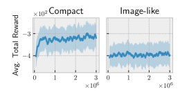
(a) $n_{p}=10,d=15,j_{s}=10$

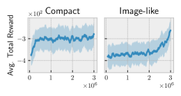
(b) $n_{p}=38,d=15,j_{s}=32$

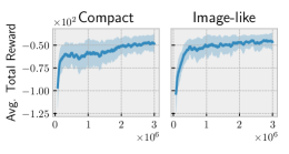
(c) $n_{p}=38,d=48,j_{s}=10$

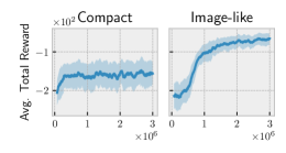
(d) $n_{p}=64,d=33,j_{s}=32$

Figure 3: Learning curves for various scenarios with $H=20$ contrasting learning using a compact representation with learning with an image-like representation. Curves are an average of six agents, with shaded areas representing one standard deviation, and show a moving average of total rewards received by the agents during training.

In Fig. 3 we show a sampling of learning curves comparing the learning performance of agents that were trained using the image-like representation and the compact representation with rewards computed from all jobs. The compact representation converges faster than the image-like representation, probably due to its smaller number of parameters. We also notice that although convergence is faster, the compact representation is not necessarily better (Fig. 3(c), 3(d)). There doesn’t seem to be a general rule, but we noticed that when jobs are shorter (the $d$ parameter is smaller), the compact representation dominates (Fig. 3(a), 3(b)). When $d$ increases and most jobs use few processors ($j_{s}\ll n_{p}$), the compact representation tends to have comparable performance with the image-like representation (Fig. 3(c)), whereas when jobs use many processors and have a longer duration, agents using the image-like representation learn the environment better (Fig. 3(d)). For this set of experiments, the size of the time horizon ($H$) doesn’t impact the learning performance, as curves obtained with $H=60$ (not shown) are indistinguishable from visual inspection to the ones obtained with $H=20$. When evaluating agents, we performed t-tests to check whether there was a difference in agent performance when using these different $H$ values. In other words, the null hypothesis was that performance was equal, and the alternative hypothesis was that agent performance varied. In this setting, the null hypothesis was rejected only $36.6\%$ of the time when considering p-values $\leq 1\%$.

Table 3: Key to the scenarios presented in Fig. 4. Procs. refers to the number of processors in the cluster, Max Length refers to the maximum job length, and Max Size refers to the maximum number of processors used by jobs.

Scenario	Procs.	Max Length	Max Size
1	10	15	10
2	10	48	10
3	38	15	32
4	38	33	32
5	38	48	32
6	64	15	64
7	64	33	32
8	64	33	64
9	64	48	32
10	64	48	64

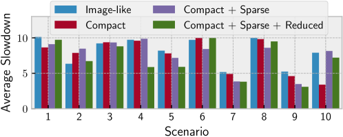
Figure 4: Average slowdown for the various scenarios considered. Each bar represents a different instantiation of the (semi-)MDPs. Average slowdowns were computed by averaging the slowdown of a thousand independent trials for each agent in each scenario. All agents were evaluated with same workload and random seed. In the legend, image-like corresponds to the base MDP, compact to the compact representation, sparse to the sparse state transitions, and reduced to the reduced set of jobs to compute rewards.

When evaluating agents after one million iterations, scheduling performance was similar between agents when the maximum number of processors used by jobs was smaller (which implies less parallelism). Given job submission rates in all environments was the same, clusters were less busy in these situations: as long as jobs are scheduled, there shouldn’t be significant differences in average slowdown, due to smaller queues.

In Fig. 4, with key to scenarions shown in Table 3, we show average slowdown of the agents for the scenarios in which there was some variability in performance between agents. From the figure, we see that, apart from scenarios 2 and 6, agent performance in the “Compact + Sparse + Reduced” MDP is not worse than that of the image-like MDP. Of these two, only the difference for scenario 6 is statistically significant, with p-value $\leq 5\%$ when performing a t-test with alternative hypothesis of different distributions. For the cases where “Compact + Sparse + Reduced” agents are better, the results are statistically significant (p-value $\leq 5\%$) in scenarios 3, 4, 5, 7, and 9. Scenarios 2 and 6 are interesting, since they were configured to have shorter jobs of at most 15 time-steps, with scenario 1 having 10 processors, and scenario 6 having 64, both with jobs with the potential of using all cluster resources.

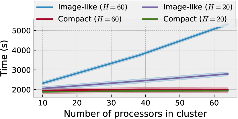
Figure 5: Time needed to train agents for three million iterations. The shaded area represents one standard deviation. Increasing the time horizon increases the training time of compact agents by a constant factor, while it adds a linear factor to the training times of agents that use an image-like representation.

In Fig. 5 we contrast the training times for the various agents. As can be seen, training times for agents based on the dense MDP are highly variable, due to the fact that different MDP configurations result in different sizes of state representations, which impacts training performance. As an example, the image-like agent requires 301068, 1089548, and 1821708 parameters for the scenarios with 10, 38, and 64 processors, while all compact agents require a fixed number of parameters: 24332. Times were measured in a Linux 5.10.42 desktop with an NVIDIA GTX 1070 GPU and an i7–8700K processor using the performance CPU frequency-scaling governor.

The compact MDPs proposed in this paper all have the characteristic of having a state representation with a fixed size, which allows for transfer of learned weights between MDPs. Here, we consider transfer the ability to change cluster configuration without the need for retraining an agent from scratch, which is simply not possible when using the image-like representation. In Figure 6, for example, we show the performance of an agent trained in the bounded reward, event-based, compact MDP with 64 processors and with jobs of length 33 (the best agent in Fig. 4, corresponding to scenario 9) evaluated in a compact environment without event-based updates. With this same agent, we were able to evaluate its performance in all different scenarios, without the need for retraining. We see that, for the most part, slowdown is kept low, and not only that: this agent outperformed other agents in 80% of scenarios (differences are statistically significant, with p-value $\leq 1\%$, except for scenario 9, since this is the same agent, and scenario 5, where the test has low power to reject the null hypothesis). This highlights the advantage of using a representation that allows for easy transfer between agents, enabling good performance in a variety of cluster settings.

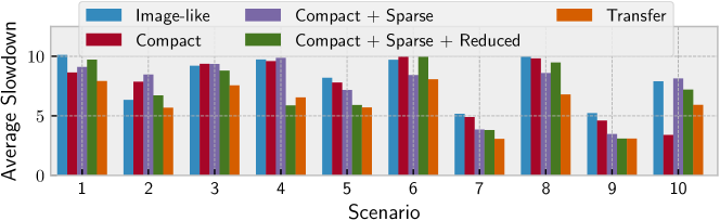
Figure 6: Bar chart contrasting the performance of a transferred agent to agents trained specifically in their environments.

6 Conclusion

In this paper, we’ve filled a gap in the literature by analyzing the effects of different MDP design decisions on the behavior of RL agents. In particular, we experimented with resource management agents for job scheduling in computing clusters, discussing cases in which a compact representation outperforms a dense one, and vice-versa. We proposed a new state representation, a transition function, and a reward function for an MDP studied in the literature, and we saw that these environments support transferring agents between different cluster settings, while also keeping agent memory consumption constant, and processing requirements stable. We also saw that these compact representations are no worse than image-like ones, and, thus, might be preferable when constant memory usage is a requirement. Moreover, our results indicate that transferred agents may outperform specialized agents in 80% of the tested scenarios without the need for retraining.

References

- Cunha et al. [2017] Renato L.F. Cunha, Eduardo R. Rodrigues, Leonardo P. Tizzei, and Marco A.S. Netto. Job placement advisor based on turnaround predictions for HPC hybrid clouds. Future Generation Computer Systems, 67:35 – 46, 2017. ISSN 0167-739X.
- de Freitas Cunha and Chaimowicz [2020] Renato Luiz de Freitas Cunha and Luiz Chaimowicz. Towards a common environment for learning scheduling algorithms. In 2020 28th International Symposium on Modeling, Analysis, and Simulation of Computer and Telecommunication Systems (MASCOTS), pages 1–8, 2020.
- Domeniconi et al. [2019] Giacomo Domeniconi, Eun Kyung Lee, and Alessandro Morari. CuSH: Cognitive ScHeduler for Heterogeneous High Performance Computing System. In Proceedings of DRL4KDD 19: Workshop on Deep Reinforcement Learning for Knowledge Discovery (DRL4KDD), volume 12, 2019.
- Fan et al. [2021] Yuping Fan, Zhiling Lan, Taylor Childers, Paul Rich, William Allcock, and Michael E Papka. Deep reinforcement agent for scheduling in hpc. arXiv preprint arXiv:2102.06243, 2021.
- Feitelson and Rudolph [1996] Dror G Feitelson and Larry Rudolph. Toward convergence in job schedulers for parallel supercomputers. In Workshop on Job Scheduling Strategies for Parallel Processing, pages 1–26. Springer, 1996.
- Liang et al. [2016] Yitao Liang, Marlos C. Machado, Erik Talvitie, and Michael Bowling. State of the Art Control of Atari Games Using Shallow Reinforcement Learning. In AAMAS, 2016.
- Mao et al. [2016] Hongzi Mao, Mohammad Alizadeh, Ishai Menache, and Srikanth Kandula. Resource management with deep reinforcement learning. In Proceedings of the 15th ACM Workshop on Hot Topics in Networks, pages 50–56, 2016.
- Mnih et al. [2016] Volodymyr Mnih, Adria Puigdomenech Badia, Mehdi Mirza, Alex Graves, Timothy Lillicrap, Tim Harley, David Silver, and Koray Kavukcuoglu. Asynchronous methods for deep reinforcement learning. In International conference on machine learning, pages 1928–1937, 2016.
- Nishida et al. [2018] Cyntia Eico Hayama Nishida, Anna Helena Reali Costa, and Reinaldo Augusto da Costa Bianchi. Control of gene regulatory networks basin of attractions with batch reinforcement learning. In 2018 7th Brazilian Conference on Intelligent Systems (BRACIS), pages 127–132, 2018.
- Raffin et al. [2019] Antonin Raffin, Ashley Hill, Maximilian Ernestus, Adam Gleave, Anssi Kanervisto, and Noah Dormann. Stable baselines3. https://github.com/DLR-RM/stable-baselines3, 2019.
- Ramos et al. [2020] Washington Ramos, Michel Silva, Edson Araujo, Leandro Soriano Marcolino, and Erickson Nascimento. Straight to the point: Fast-forwarding videos via reinforcement learning using textual data. In Proceedings of the IEEE/CVF Conference on Computer Vision and Pattern Recognition, pages 10931–10940, 2020.
- Schulman et al. [2017] John Schulman, Filip Wolski, Prafulla Dhariwal, Alec Radford, and Oleg Klimov. Proximal policy optimization algorithms. arXiv preprint arXiv:1707.06347, 2017.
- Silver et al. [2018] David Silver, Thomas Hubert, Julian Schrittwieser, Ioannis Antonoglou, Matthew Lai, Arthur Guez, Marc Lanctot, Laurent Sifre, Dharshan Kumaran, Thore Graepel, et al. A general reinforcement learning algorithm that masters chess, shogi, and Go through self-play. Science, 362(6419):1140–1144, 2018.
- Sutton et al. [1999] Richard S. Sutton, Doina Precup, and Satinder Singh. Between MDPs and semi-MDPs: A framework for temporal abstraction in reinforcement learning. Artificial Intelligence, 112(1):181–211, 1999. ISSN 0004-3702. doi: https://doi.org/10.1016/S0004-3702(99)00052-1.
- Tesauro [1994] Gerald Tesauro. TD-Gammon, a self-teaching backgammon program, achieves master-level play. Neural computation, 6(2):215–219, 1994.
- Zhang et al. [2020] Di Zhang, Dong Dai, Youbiao He, Forrest Sheng Bao, and Bing Xie. Rlscheduler: an automated hpc batch job scheduler using reinforcement learning. In SC20: International Conference for High Performance Computing, Networking, Storage and Analysis, pages 1–15. IEEE, 2020.