Infusing Future Information into Monotonic Attention Through Language Models

Abstract

Simultaneous neural machine translation (SNMT) models start emitting the target sequence before they have processed the source sequence. The recent adaptive policies for SNMT use monotonic attention to perform read/write decisions based on the partial source and target sequences. The lack of sufficient information might cause the monotonic attention to take poor read/write decisions, which in turn negatively affects the performance of the SNMT model. On the other hand, human translators make better read/write decisions since they can anticipate the immediate future words using linguistic information and domain knowledge. Motivated by human translators, in this work, we propose a framework to aid monotonic attention with an external language model to improve its decisions. We conduct experiments on the MuST-C English-German and English-French speech-to-text translation tasks to show the effectiveness of the proposed framework. The proposed SNMT method improves the quality-latency trade-off over the state-of-the-art monotonic multihead attention.

1 Introduction

Simultaneous Neural Machine Translation (SNMT) addresses the problem of real-time interpretation in machine translation. A typical application of real-time translation is conversational speech or live video caption translation. In order to achieve live translation, an SNMT model alternates between reading from the source sequence and writing to the target sequence using either a fixed or an adaptive read/write policy.

The fixed policies Ma et al. (2019a) may introduce too much delay for some examples or not enough for others. The recent works focus on training adaptive policies using techniques such as monotonic attention. There are several variants of monotonic attention: hard monotonic attention Raffel et al. (2017), monotonic chunkwise attention Chiu* and Raffel* (2018), monotonic infinite lookback attention (MILk) Arivazhagan et al. (2019), and monotonic multihead attention (MMA) Ma et al. (2019b). These monotonic attention processes can anticipate target words using only the available prefix source and target sequence. However, human translators anticipate the target words using their language expertise (linguistic anticipation) and contextual information (extra-linguistic anticipation) Vandepitte (2001) as well.

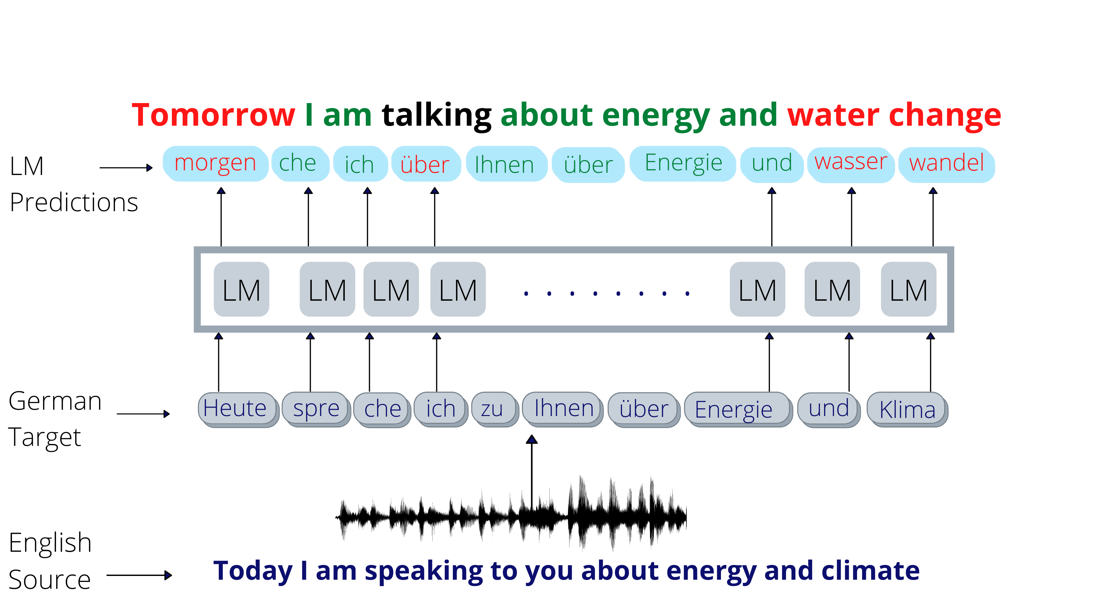
Figure 1: The finetuned XLM-Roberta language model predicts German words using the prefix as input.
(Green: Correct, Red: Incorrect, Black: Neutral).

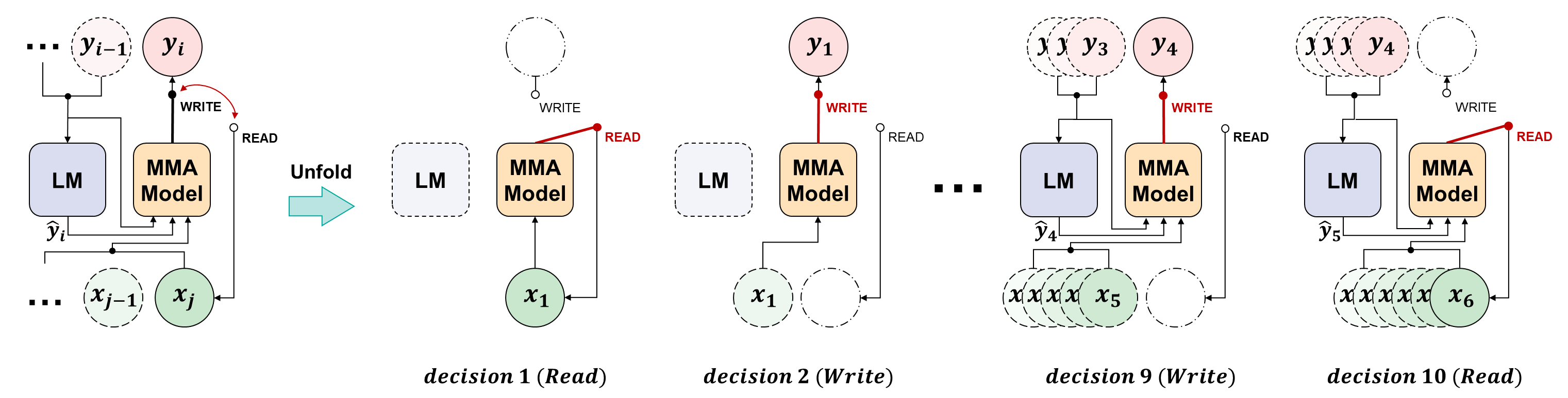
Figure 2: Overview of the simultaneous translation model with future information.

Motivated by human translation experts, we aim to augment monotonic attention with linguistic and extra-linguistic information. We propose to use language model (LM) to obtain the above-mentioned future information. As shown in Figure 1, at each step, the LM takes the prefix target (and source, for cross-lingual LM) sequence and predicts the plausible future information. We hypothesize that aiding the monotonic attention with this future information might help the SNMT model improve the latency-quality trade-off.

The main contributions of this paper are: (1) A novel monotonic attention mechanism to leverage the future information (2) Improved latency-quality trade-offs compared to the state-of-the-art MMA models on MUST-C Di Gangi et al. (2019) English-German and English-French speech-to-text translation tasks. (3) Analyses on how our proposed monotonic attention achieves superior performance over MMA and LM rescoring-based MMA. We also analyze the performance of the proposed framework with custom and general-purpose LM.

2 Monotonic Attention with Future Information Model

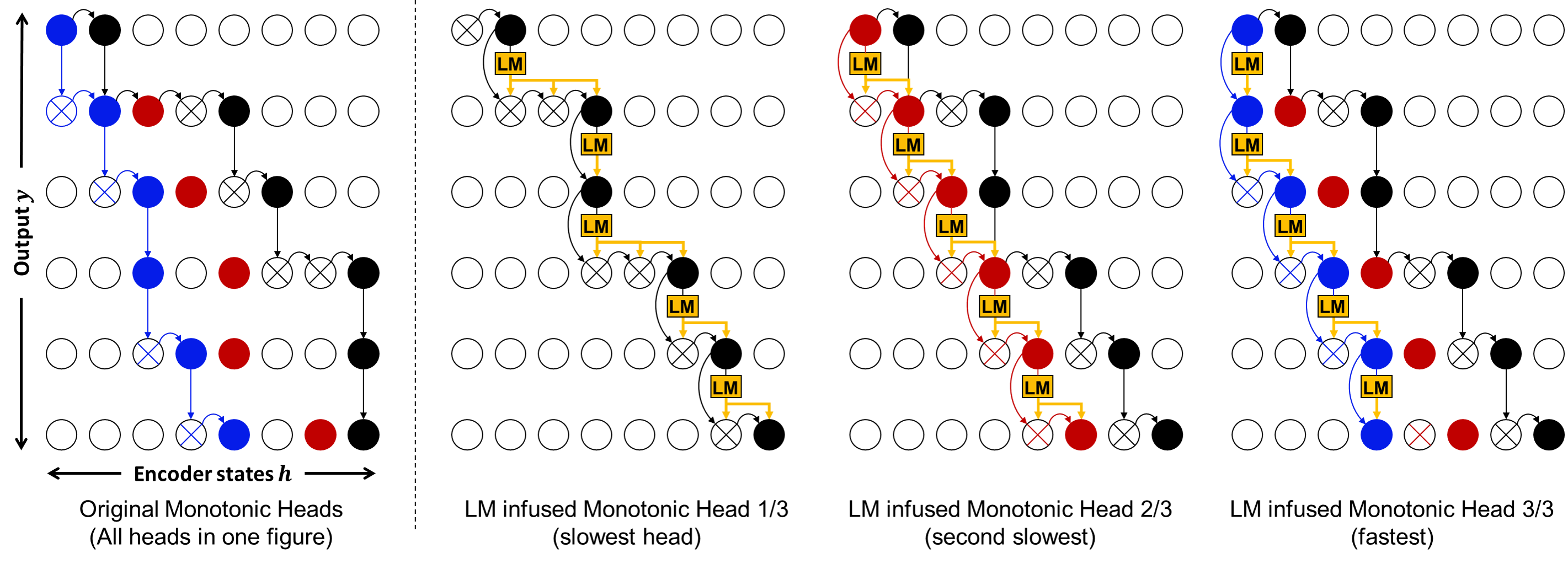
Figure 3: Overview of the monotonic multihead attention with future information.

1 Input: Training examples, $E=\{x^{n},y^{n}\}_{n=1}^{N}$, hyperparameters such as learning rate ($\alpha$), $\lambda$ (latency), language model (LM)

2Extract plausible future information using LM, $\hat{y}_{i}^{n}=LM({y_{1}^{n},\cdots,y_{i-1}^{n}})\quad\forall i,n$

3Append each $\hat{y}^{n}$ information to target sequence $y^{n}$. New target sequence $\bar{y}^{n}=\{(y_{1}^{n},\hat{y}_{1}^{n}),(y_{2}^{n},\hat{y}_{2}^{n}),\cdots,(y_{|y|}^{n},\emptyset)\}$

4Modified training examples are $\bar{E}=\{x^{n},\bar{y}^{n}\}_{n=1}^{N}$

5Initialize model parameters $\theta$

6while training is not done do

7       Sample a training example(s) from $\bar{E}$

8      compute $\{h_{1},\cdots,h_{|x|}\}$ for $x$ (Eq. 1)

9      tokenize $y$ and $\hat{y}_{i}$

10      Run a sub-token summary layer ( Eq. 13) on $\hat{y})$ , to obtain $\tilde{\mathbf{y}_{i}}$ for each $\mathbf{y}_{i-1}$

11      for each decoding step do

12             Compute monotonic energy and future monotonic energy for $\mathbf{y}_{i-1}$, $\tilde{\mathbf{y}_{i}}$ (Eq. 8 and 15)

13            Compute read/write decision (Eq. 16)

14            compute context vector $c_{i}$ (Eq. 12), and output target token (Eq. 2, 3)

15       end for

16      Compute the latency loss along with negative log likelihood

17      Update $\theta$ with gradient descent

18 end while

19

20Return: $\theta$

Algorithm 1 Monotonic Attention with Future Information

2.1 Monotonic Attention

The source and the target sequences are represented as $\mathbf{x}=\{x_{1},x_{2},\cdots,x_{S}\}$ and $\mathbf{y}=\{y_{1},y_{2},\cdots,y_{T}\}$, with $S$ and $T$ being the length of the source and the target sequences. The simultaneous machine translation models (SNMT) produce the target sequence concurrently with the growing source sequence. In other words, the probability of predicting the target token $y_{i}\in\mathbf{y}$ depends on the partial source and target sequences ($x_{\leq j}\in\mathbf{x},y_{<i}\in\mathbf{y}$). In this work, we consider sequence-to-sequence based SNMT model in which each target token $y_{i}$ is generated as follows:

$$h_{j}=\mathcal{E}(x_{\leq j})$$ (1)

$$s_{i}=\mathcal{D}(y_{<i},c_{i})$$ (2)

$$y_{i}=Output(s_{i})$$ (3)

where $\mathcal{E}(.)$ and $\mathcal{D}(.)$ are the Transformer Vaswani et al. (2017) encoder and decoder layers, and $c_{i}$ is a context vector. In offline MT, the context vector is computed using a soft attention mechanism Bahdanau et al. (2015). In monotonic attention based SNMT, the context vector is computed as follows:

$$e_{i,j}=MonotonicEnergy(y_{i-1},h_{j})$$ (4)

$$p_{i,j}=Sigmoid(e_{i,j})$$ (5)

$$z_{i,j}\sim Bernoulli(p_{i,j})$$ (6)

When generating a new target token $y_{i}$, the decoder chooses whether to read/write based on Bernoulli selection probability $p_{i,j}$. When $z_{i,j}=1$, we set $t_{i}=j$, $c_{i}=h_{j}$ (write) and generate the target token $y_{i}$; otherwise, we set $t_{i}=j+1$ (read) and repeat Eq. 4 to 6. Here $t_{i}$ refers to the index of the encoder entry needed to produce the $i^{th}$ target token. Instead of hard assignment of $c_{i}=h_{j}$, Raffel et al. (2017) compute an expected alignment $\boldsymbol{\alpha}$ which can be calculated in a recurrent manner as shown in Eq. 7:

$$\alpha_{i,j} =p_{i,j}\sum_{k=1}^{j}\left(\alpha_{i-1,k}\prod_{l=k}^{j-1}(1-p_{i,l})\right)$$

$$=p_{i,j}\left((1-p_{i,j-1})\frac{\alpha_{i,j-1}}{p_{i,j}}+\alpha_{i-1,j}\right)$$ (7)

Raffel et al. (2017) also propose a closed-form parallel solution that allows $\alpha_{i,j}$ to be computed for all $j$ in parallel using cumulative sum and cumulative product operations. Arivazhagan et al. (2019) propose Monotonic Infinite Lookback Attention (MILk), which combines the soft attention with monotonic attention to attend all the encoder states from the beginning of the source sequence till $t_{i}$ for each $y_{i}$. Ma et al. (2019b) extends MILk to monotonic multihead attention (MMA) to integrate it into the Transformer model Vaswani et al. (2017).

The MMA model implements the monotonic energy function in Eq. 4 through scaled-dot product attention. For a Transformer model with $L$ decoder layers and $H$ attention heads per layer, the energy function of a $h$-th head encoder-decoder attention in the $l$-th decoder layer is computed as follows:

$$e_{i,j}^{l,h}=\left(\frac{h_{j}W_{l,h}^{K}(\mathbf{y}_{i-1}W_{l,h}^{Q})^{T}}{\sqrt{d_{k}}}\right)_{i,j}$$ (8)

$$p_{i,j}^{l,h}=Sigmoid(e_{i,j}^{l,h})$$ (9)

where $W_{l,h}^{K}$ and $W_{l,h}^{Q}$ are the projection matrices for $h_{j}$ and $\mathbf{y}_{i-1}$, $\mathbf{y}_{i-1}$ is the representation of the previous output token and $d_{k}$ is the dimension of the attention head.

The MMA attention for each head is calculated as follows:

$$u_{i,o}^{l,h}=\left(\frac{h_{o}W_{l,h}^{K}(y_{i-1}W_{l,h}^{Q})^{T}}{\sqrt{d_{k}}}\right)_{i,j},o\in 1,2,\cdots,t_{i}$$ (10)

$$\beta_{i,j}=\sum_{k=j}^{|x|}\left(\frac{\alpha_{i,k}exp(u_{i,j})}{\sum_{n=1}^{k}exp(u_{i,n})}\right)$$ (11)

$$c_{i}=\sum_{j=1}^{|x|}\beta_{i,j}h_{j}$$ (12)

The attention mechanisms in MILk and MMA encourage the model to output the target token with limited source information by adding latency loss metrics to the training objective. Please refer to Arivazhagan et al. (2019) and Ma et al. (2019b) for more details.

2.2 Monotonic Attention with Future Information

The monotonic attention described in Section 2.1 performs anticipation based only on the currently available source and target information. We propose to use linguistic and extra-linguistic information, similar to human interpreters, to improve the performance of the SNMT model.

In order to get the future information for monotonic attention, we rely on LMs, which can inherently provide linguistic information. The extra-linguistic information is also obtained when the LM is finetuned on a particular task. To incorporate the future information, we propose the following modifications to the monotonic attention.

2.2.1 Future Representation Layer

At every decoding step $i$, the previous target token $y_{i-1}$ is equipped with a plausible future token $\hat{y}_{i}$ as shown in the Figure 2. Since the token $\hat{y}_{i}$ comes from an LM possibly with a different tokenizer and vocabulary set, applying the model’s tokenizer and vocabulary might split the token $\hat{y}_{i}$ further into multiple sub-tokens $\{\hat{y}_{i}^{1},\hat{y}_{i}^{2},\cdots,\hat{y}_{i}^{m}\}$. To get a single future token representation $\tilde{\textbf{y}}_{i}\in\mathcal{R}^{d}$ from all the sub-tokens, we apply a sub-token summary layer as follows:

$$\tilde{\textbf{y}}_{i}=\Gamma(\{\hat{y}_{i}^{1},\hat{y}_{i}^{2},\cdots,\hat{y}_{i}^{m}\})$$ (13)

The $\Gamma$ represents a general sequence representation layer such as a Transformer encoder layer or a simple normalized sum of sub-token representations.

We enrich $\tilde{\textbf{y}}_{i}$ at every layer $l$ of the decoder block by applying a residual-feed forward network similar to the final sub-layer in the transformer decoder block.

$$\tilde{\mathbf{y}}_{i}^{l}=FFN(\tilde{\mathbf{y}}_{i}^{l-1})$$ (14)

2.2.2 Monotonic Energy Layer with Future Information

We can add the plausible future information to the output layer or append it to the target token representation $y_{i-1}$. However, the MMA read/write decisions happen in Eq. 8, therefore, we integrate $\tilde{\mathbf{y}}_{i}$ into the Eq. 8. This way of integration of plausible future information allows the model to condition the LM output usage on the input speech. Hence, it can choose to discard incorrect information. The integration is carried out by modifying Eq. 4 - Eq. 9 in the following way:

First, we compute the monotonic energy for future information using the enriched future token representation $\tilde{\mathbf{y}}_{i}^{l}$ available at each layer:

$$\tilde{e}_{i,j}^{l}=\left(\frac{h_{j}\tilde{W}_{l}^{K}(\tilde{\mathbf{y}}_{i}\tilde{W}_{l}^{Q})^{T}}{\sqrt{d}}\right)_{i,j}$$ (15)

where $\tilde{W}_{l}^{K}$ and $\tilde{W}_{l}^{Q}$ are the projection matrices for $h_{j}$ and $\tilde{\mathbf{y}}_{i}$, and $d_{k}$ is the dimension of the attention head of Eq. 8.

We integrate the future monotonic energy function into Eq. 9 as follows:

$$\tilde{p}_{i,j}^{l,h}=\Omega(e_{i,j}^{l,h},\tilde{e}_{i,j}^{l})$$ (16)

$\Omega$ represents a general modulation operator and can be replaced with feature-wise linear modulation Perez et al. (2018) or multiplicative or additive operations. As shown in Figure 3, during training, each head in the monotonic energy $e_{i,j}^{l,h}$ sees the same future monotonic energy $\tilde{e}_{i,j}^{l}$, since during the inference of multihead monotonic attention, the write operation depends on the slowest head.

After computing $\tilde{p}_{i,j}^{l,h}$, we compute $c_{i}$ using Eq. 12. The overall process is described in Algorithm 1. In our experiments, we use the MMA-Infinite Lookback attention model, but our algorithm can be easily extended for MMA-H by modifying the context vector computation to choose only one encoder state.

2.2.3 Inference

During the inference time, the start token does not contain any plausible information. After predicting the first target token, for every subsequent prediction of target token $y_{i}$, we invoke the LM to predict the next plausible future token. Whenever new source information arrives, we run step 8 of Algorithm 1. Similarly, for every new target token prediction, we extract new plausible future information from LM using the available predicted sequence, and then we run step 9 to 14 of the Algorithm 1.

3 Experiments

3.1 Datasets and Metrics

We conduct our experiments on the English(En)-German(De) and English(En)-French(Fr) speech-to-text (ST) translation task. These tasks are more involved compared to the text-to-text translations since these are low resource tasks. Moreover, due to different input-output modalities, the difference in source and target sequence lengths is larger compared to the text-to-text task. We use the EnDe, and EnFr portions of the MuST-C dataset. We use the MuST-C dev set for validation and tst-COMMON test set for evaluation. More details about the datasets have been provided in the Appendix.

The speech sequence is represented using 80-dimensional log mel features extracted using the KaldiPovey et al. (2011) toolkit with a 25ms window size and 10ms shift. The target sequence is represented as subwords using a SentencePiece Kudo and Richardson (2018) model with a unigram vocabulary of size 10,000. We evaluate the performance of the models on both the latency and quality aspects. We use Average Lagging(AL) as our latency metric and case-sensitive detokenized SacreBLEU Post (2018) to measure the translation quality, similar to Ma et al. (2020b). The best models are chosen based on the dev set results and reported results are computed using the MuST-C test sets.

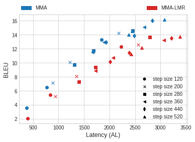
(a) EnDe Task

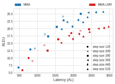
(b) EnFr Task

Figure 4: BLEU vs Average Lagging results for MMA and MMA-LMR models

3.2 Implementation Details

Our base model is adopted from Ma et al. (2020b) and the initial implementation is taken from Fairseq repository. In the text-to-text case, each encoder state corresponds to a vocabulary unit. Hence, the read/write decisions are taken for each encoder state. For Simultaneous ST, each encoder state represents only 40ms of speech, assuming a sub-sampling factor of 4 from the convolutional layers. We use a pre-decision ratio of 7 (segment size of 280ms), which means that the simultaneous read/write decisions are made after every seven encoder states, which roughly corresponds to a word(average word length for the EnDe dataset is 270ms Ma et al. (2020b)). Since we train MMA-IL Ma et al. (2019b) models, we set $\lambda_{var}=0$ for all our experiments as it was not reported to be helpful for models with infinite lookback. We use $\lambda$ or $\lambda_{latency}$ to refer to the hyperparameter corresponding to the weighted average($\lambda_{avg}$) in MMA. The values of this hyperparameter $\lambda$ are chosen from the set $\{0.01,0.05,0.1\}$. The $\Gamma$ layer in Eq. 13 computes the normalized sum of the sub-token representations. For SLM, it simply finds the embedding since it shares the same vocabulary set. The $\Omega$ layer in Eq. 16 performs the additive operation to add the energies corresponding to previous output token $y_{i-1}$ and the prediction $\hat{y}_{i}$. All the models were trained by simulating 8 GPU settings on a single NVIDIA v100 GPU.

3.3 Models

We train a baseline model based on Ma et al. (2020b), called the MMA model. The base MMA model encoder and decoder embedding dimensions are set to 392, whereas our proposed model’s encoder and decoder embeddings are set to 256 to have similar parameters ($\approx 39M$) for a fairer comparison. Apart from the encoder and decoder embedding dimension difference, all other hyperparameter settings and training procedures are similar for all the reported models. We train two MMA models based on two different LMs used for extracting future information. Details have been provided in Section 3.4.

We explored a naive approach of integrating LM information into the MMA. We modify the baseline MMA inference process to integrate the information from the LM. Instead of greedy decoding, we evaluate the top-5 outputs from the MMA at each decoding step using the LM. We use the perplexity score provided by the LM to rank the partial predicted sentences formed using these top-5 outputs and choose the best one. The advantage of this approach is that we do not need to modify the training process of the MMA model. We refer to this experiment as ’LM Rescoring(LMR)’, and the corresponding model is called MMA-LMR.

We follow the training process similar to Ma et al. (2020b) training process. We train an English ASR model using the source speech data. Next, we train a simultaneous model without the latency loss (setting $\lambda_{latency}=0$) after initializing the encoder from the English ASR model. After this step, we finetune the simultaneous model for different $\lambda$s. This training process is repeated for all the reported models and for each task.

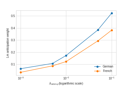
Figure 5: LM prediction weight vs $\lambda$

3.4 Language Model

We use two different language models to train our proposed LM-based simultaneous speech translation model. Firstly, we use the pretrained XLM-RoBERTa Conneau et al. (2019) model from Huggingface Transformers model repository. It is a multilingual(more than 100 languages) LM trained on a wide variety of cross-lingual tasks. The model contains 550M parameters with 24 layers, 1,024 hidden-states. Since the LM output can be very open-ended and might not directly suit/cater to our task and dataset, we finetune the head of the model using the target MuST-C text data corresponding to each task.

We also train a smaller language model(SLM), which contains 6 Transformer decoder layers, 512 hidden-states and 24M parameters. We use the MuST-C data along with additional data augmentation to reduce overfitting. Although trained on a much smaller monolingual dataset, it helps to remove the issues related to vocabulary mismatch as discussed in the Section 2.2.1. This LM has lower inference time and has higher accuracy on the next token prediction task as compared to XLM, 30.15% vs. 21.5% for German & 31.65% vs. 18.45% for French. More details about LMs have been provided in the Appendix. The models trained using these LMs are referred to as MMA-XLM and MMA-SLM.

3.5 Results

In this section, we first provide the results for the MMA-LMR model. The results for MMA-XLM and MMA-SLM have been provided in the form of latency-quality trade-off curves. Finally, we provide analysis and explanation for the results.

LM based Rescoring

For MMA-LMR, we use the LM only during inference. As observed in Figure 4, MMA-LMR has inferior performance compared to the MMA model. Since the LM information integration is not conditioned on the input speech, the MMA model cannot discard the incorrect information from LM. This motivates us to tightly integrate the LM information into the simultaneous model.

Latency-Quality Curves

We obtain several simultaneous models based on MMA, MMA-XLM, MMA-SLM systems by using different latencies ($\lambda$) during training and different speech segment sizes during inference. The speech segment size refers to the duration of speech(in ms) processed corresponding to each read decision. We plot the BLEU scores against the Average Lagging(AL) incurred during the evaluation using SimulEval toolkitMa et al. (2020a). The BLEU-AL curves for all the models have been provided in Figure 6. We can observe that the LM-based models provide a better translation quality at the same latency or lower latency for the same translation quality or some times improving in both aspects

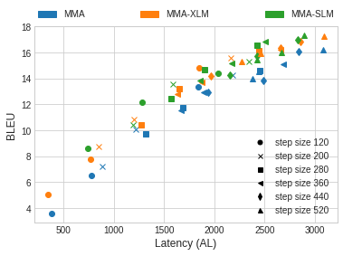
(a) EnDe Task

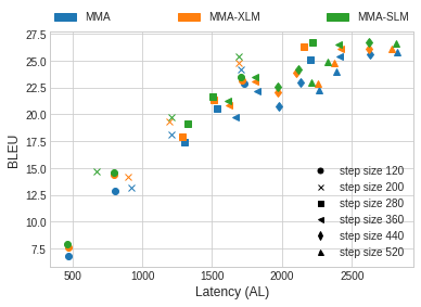
(b) EnFr Task

Figure 6: BLEU vs Average Lagging results for MMA, MMA-XLM and MMA-SLM models. MMA-XLM and MMA-SLM provide better latency/quality tradeoff curves.

LM anticipation vs Latency

In order to measure the relative weight given to the predictions from the LM, we compare the norm of the monotonic energies corresponding to the LM predictions $e_{pred}$(Eq. 15) and the previous output tokens $e_{output}$(Eq. 8 ). Let us define LM prediction weight as

$$LM_{pw}=\left(\frac{\left\lVert e_{pred}\right\rVert}{\left\lVert e_{output}\right\rVert}\right)$$ (17)

In Figure 5, we plot the variation of $LM_{pw}$(averaged) vs. ${\lambda}$. We can observe that as the latency requirements become more and more strict, the model starts to give more weightage to the predictions coming from the LM. In other words, as the need for anticipation increases, the model starts to rely more on the LM predictions.

Effect of LM Size on CAAL

As we can observe from the Figure 6, the results for MMA-XLM and MMA-SLM are very close. Not only does MMA-SLM perform slightly better than MMA-XLM, but the prediction computation time is also much lower since XLM is much deeper than SLM. The average time taken to compute one token during prediction for SLM is 6.1ms as compared to 24.78ms for XLM. However, XLM is more suitable for multilingual settings since we can use same LM for all the languages.

In order to account for the computation time incurred by the model, we also use the Computation Aware Average Latency (CAAL) introduced in Ma et al. (2020b). AL(non-computation aware) is measured in terms of the duration of speech listened to before generating target token, while CAAL uses the wall-clock time, which also factors in the time elapsed due to the model complexity. In Figure 7, we provide the CAAL for various $\lambda$ values for approximately similar BLEU. For a given value of AL, LM based MMA models have a higher CAAL when compared to the MMA model. This gap is expected and occurs due to the time taken for the LM to compute the predictions. However, both MMA-XLM and MMA-SLM improve the latency-quality trade-off and hence reduce the AL for a given BLEU. As observed, MMA-SLM has lesser CAAL as compared to MMA since the extra computation time is balanced by the reductions in AL due to the algorithmic improvements. MMA-XLM, on the other hand, has a slightly higher CAAL. English speakers utter 6.2 syllables per secPellegrino et al. (2011), which means 160ms/syllable. Both German and French readers read roughly 5 syllables/sec, 200ms/syllable Trauzettel-Klosinski et al. (2012). Considering this human perception speed, a gap of 6 or 24ms per sub-word(which might contain multiple syllables) should not cause acute deterioration in the user experience.

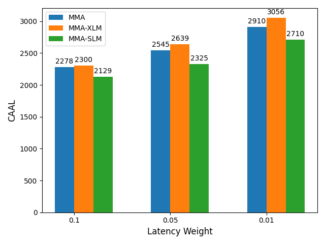
(a) EnDe Task

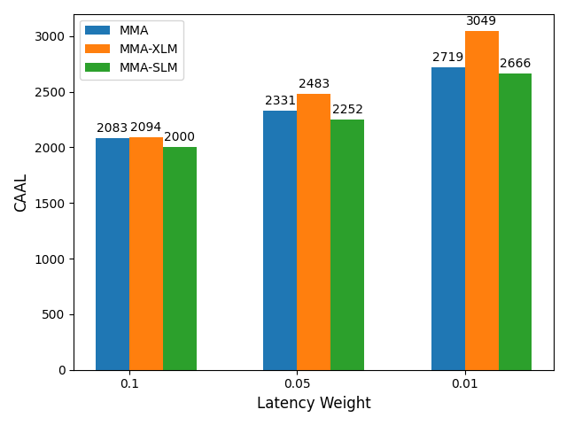
(b) EnFr Task

Figure 7: Computational aware latency of MMA, MMA-XLM, MMA-SLM with similar BLEU scores and different latencies={0.1, 0.05, 0.01}

4 Related Work

The earlier works in streaming simultaneous translation such as Cho and Esipova (2016); Gu et al. (2016); Press and Smith (2018) lack the ability to anticipate the words with missing source context. Ma et al. (2019a) established a more sophisticated approach by integrating their read/write agent directly into MT. Similar to Dalvi et al. (2018), they employ a fixed agent that first reads $k$ source tokens and then proceeds to alternate between write and read until the source tokens are finished. Recently, the adaptive policies based on several variants of monotonic attention for SNMT have been explored: hard monotonic attention Raffel et al. (2017), monotonic chunkwise attention (MoChA) Chiu* and Raffel* (2018) and monotonic infinite lookback attention (MILk) Arivazhagan et al. (2019). MILK improves upon the wait-k training with an attention that can adapt how it will wait based on the current context. Monotonic multihead attention (MMA) Ma et al. (2019b) extends MILk to transformer-based models.

Gulcehre et al. (2015, 2017) propose shallow fusion of language models(LMs) into text-to-text machine translation(MT) by combining LM and MT scores at inference time using a log-linear model. However, this has a mismatch between training and inference of MT. To overcome this drawback, Stahlberg et al. (2018) integrate the LM scores during MT training. They use a pretrained LM and train the MT system to optimize the combined score of LM and MT on the training set. Sriram et al. (2018) explored a similar idea for Automatic Speech Recognition(ASR) using a gating network for controlling the relative contribution of the LM. These techniques allow the main sequence to sequence model(either ASR or MT) to focus on modeling the source sentence, while the LM controls the target side generation. Wu et al. (2020) implicitly uses future information during training of SNMT systems by simultaneously training different wait-k systems. The translation model is jointly trained with a controller model that decides which $k$ is optimal to use for training a particular batch of examples. However, they do not use any explicit future information during training and inference.

End-to-end speech translation Indurthi et al. (2020); Sperber and Paulik (2020) has recently made great progress and even surpassed the cascaded models (ASR followed by MT) Ney (1999); Post et al. (2013). Recently, Ren et al. (2020) investigate how to adapt the simultaneous models for speech-to-text translation tasks. Han et al. (2020) use meta-learning algorithm Finn et al. (2017) and improve these wait-k based simultaneous speech-to-text models. Ma et al. (2020b) explore the usage of monotonic multihead attention by introducing a pre-decision module.

5 Conclusion

In this work, we provide a generic framework to integrate the linguistic and extra-linguistic information into simultaneous models. This information helps to improve the anticipation for monotonic attention based SNMT models. We rely on language models to extract plausible future information and propose a new monotonic attention mechanism to infuse future information. We conduct several experiments on low resource speech-to-text translation tasks to show the effectiveness of proposed approach. We have achieved superior quality-latency trade-off compared to the state-of-the-art monotonic multihead attention. In the future work, we plan to extend the proposed framework to the text-to-text simultaneous translation and analyze different future information fusion mechanisms.

Task	# Hours	# Sentences			# Talks	# Words
		Train	Dev	Test		Source	Target
English-German	408	225k	1,423	2,641	2,093	4.3M	4M
English-French	492	269k	1,412	2,632	2,510	5.2M	5.4M

Table 1: Dataset Statistics(# - Number of)

	MMA	MMA-XLM/CLM
Hyperparameter
encoder layers	12	12
encoder embed dim	292	256
encoder ffn embed dim	2048	2048
encoder attention heads	4	4
decoder layers	6	6
decoder embed dim	292	256
decoder ffn embed dim	2048	2048
monotonic ffn embde dim	–	2048
decoder attention heads	4	4
dropout	0.1	0.1
optimizer	adam	adam
adam-$\beta$	(0.9, 0.999)	(0.9, 0.999)
clip-norm	10.0	10.0
lr scheduler	inverse sqrt	inverse sqrt
learning rate	0.0001	0.0001
warmup-updates	4000	4000
label-smoothing	0.0	0.0
max tokens	40000	40000
conv layers	2	2
conv stride	(2,2)	(2,2)
#params	$\approx 39M$	$\approx 39M$

Table 2: Model Hyperparameters

Appendix A Language Models

As mentioned earlier, we train two different language models (LMs) and use them to improve the anticipation in monotonic attention based Simultaneous models.

A.1 XLM-Roberta(XLM-R)

XLM-R Large model was trained on the 100 languages CommonCrawl corpora total size of 2.5TB with 550M parameters from 24 layers, 1024 hidden states, 4096 feed-forward hidden-states, and 16 heads. Total number of parameters is 558M. We finetune the head of the XLM-R LM model using the Masked Language Modeling objective which accounts for 0.23% of the total model parameters, i.e., 1.3M parameters.

A.2 Smaller Language Model

Since the LM predictions are computed serially during inference, the time taken to compute the LM token serves as a bottleneck to the latency requirements. To reduce the LM computation time, we train a smaller Language Model (SLM) from scratch using the Causal Language Modeling objective. SLM is composed of 6 Transformer decoder blocks, 512 hidden-states, 2048 feed-forward hidden-states & 8 attention heads. It alleviates the need for the sub-token summary layer since it shares the vocabulary and tokenization with the MMA models. The train examples are at the sentence level, rather than forming a block out of multiple sentences(which is the usual case for Language Models).

Since the target texts contain lesser than 250k examples, we use additional data augmentation techniques to upsample the target data. We also use additional data to avoid overfitting on the MuST-C target text. Details have been provided in A.2.1.

A.2.1 Data Augmentation

Up-Sampling:

To boost the LM performance and mitigate overfitting, we use contextual data augmentation Kobayashi (2018) to upsample the MuST-C target text data by substituting and inserting words based on LM predictions. We use the NLPAUG package to get similar words based on contextual embeddings. From the Hugging Face Repository, we use two different pretrained BERT Devlin et al. (2019) models for German bert-base-german-dbmdz-cased & bert-base-german-dbmdz-uncased and bert-base-fr-cased for French. We upsample German to 1.13M examples and French to 1.38M examples.

Additional Data:

We also use additional data to avoid overfitting. For German we use the Newscrawl(WMT 19) data which includes 58M examples. For French, we use Common Crawl and Europarl to augment 4M extra training examples.

We observe that both upsampling and data augmentation help us to reduce the overfitting on the MuST-C dev set.

A.3 Token Prediction

For each output token, the LM prediction is obtained by feeding the prefix upto that token to the LM model. These predictions are pre-computed for training and validation sets. This ensures parallelization and avoids the overhead to run the LM simultaneously during the training process. During inference, the LM model is called every time a new output token is written.

Appendix B Dataset

The MuST-C dataset comprises of English TED talks, the translations and transcriptions have been aligned with the speech at sentence level. Dataset statistics have been provided in the Table 1.

Appendix C Hyperparameters

The details regarding the hyperparameters for the model have been provided in Table 2.

References

- Arivazhagan et al. (2019) Naveen Arivazhagan, Colin Cherry, Wolfgang Macherey, Chung-Cheng Chiu, Semih Yavuz, Ruoming Pang, Wei Li, and Colin Raffel. 2019. Monotonic infinite lookback attention for simultaneous machine translation. In Proceedings of the 57th Annual Meeting of the Association for Computational Linguistics, pages 1313–1323, Florence, Italy. Association for Computational Linguistics.
- Bahdanau et al. (2015) Dzmitry Bahdanau, Kyunghyun Cho, and Yoshua Bengio. 2015. Neural machine translation by jointly learning to align and translate.
- Chiu* and Raffel* (2018) Chung-Cheng Chiu* and Colin Raffel*. 2018. Monotonic chunkwise attention. In International Conference on Learning Representations.
- Cho and Esipova (2016) Kyunghyun Cho and Masha Esipova. 2016. Can neural machine translation do simultaneous translation? arXiv preprint arXiv:1606.02012.
- Conneau et al. (2019) Alexis Conneau, Kartikay Khandelwal, Naman Goyal, Vishrav Chaudhary, Guillaume Wenzek, Francisco Guzmán, Edouard Grave, Myle Ott, Luke Zettlemoyer, and Veselin Stoyanov. 2019. Unsupervised cross-lingual representation learning at scale. arXiv preprint arXiv:1911.02116.
- Dalvi et al. (2018) Fahim Dalvi, Nadir Durrani, Hassan Sajjad, and Stephan Vogel. 2018. Incremental decoding and training methods for simultaneous translation in neural machine translation. In Proceedings of the 2018 Conference of the North American Chapter of the Association for Computational Linguistics: Human Language Technologies, Volume 2 (Short Papers), pages 493–499, New Orleans, Louisiana. Association for Computational Linguistics.
- Devlin et al. (2019) Jacob Devlin, Ming-Wei Chang, Kenton Lee, and Kristina Toutanova. 2019. BERT: Pre-training of deep bidirectional transformers for language understanding. In Proceedings of the 2019 Conference of the North American Chapter of the Association for Computational Linguistics: Human Language Technologies, Volume 1 (Long and Short Papers), pages 4171–4186, Minneapolis, Minnesota. Association for Computational Linguistics.
- Di Gangi et al. (2019) Mattia A. Di Gangi, Roldano Cattoni, Luisa Bentivogli, Matteo Negri, and Marco Turchi. 2019. MuST-C: a Multilingual Speech Translation Corpus. In Proceedings of the 2019 Conference of the North American Chapter of the Association for Computational Linguistics: Human Language Technologies, Volume 1 (Long and Short Papers), pages 2012–2017, Minneapolis, Minnesota. Association for Computational Linguistics.
- Finn et al. (2017) Chelsea Finn, Pieter Abbeel, and Sergey Levine. 2017. Model-agnostic meta-learning for fast adaptation of deep networks. In Proceedings of the 34th International Conference on Machine Learning, volume 70 of Proceedings of Machine Learning Research, pages 1126–1135. PMLR.
- Gu et al. (2016) Jiatao Gu, Graham Neubig, Kyunghyun Cho, and Victor OK Li. 2016. Learning to translate in real-time with neural machine translation. arXiv preprint arXiv:1610.00388.
- Gulcehre et al. (2015) Caglar Gulcehre, Orhan Firat, Kelvin Xu, Kyunghyun Cho, Loic Barrault, Huei-Chi Lin, Fethi Bougares, Holger Schwenk, and Yoshua Bengio. 2015. On using monolingual corpora in neural machine translation.
- Gulcehre et al. (2017) Caglar Gulcehre, Orhan Firat, Kelvin Xu, Kyunghyun Cho, and Yoshua Bengio. 2017. On integrating a language model into neural machine translation. Computer Speech and Language, 45:137–148.
- Han et al. (2020) Hou Jeung Han, Mohd Abbas Zaidi, Sathish Reddy Indurthi, Nikhil Kumar Lakumarapu, Beomseok Lee, and Sangha Kim. 2020. End-to-end simultaneous translation system for IWSLT2020 using modality agnostic meta-learning. In Proceedings of the 17th International Conference on Spoken Language Translation, pages 62–68, Online. Association for Computational Linguistics.
- Indurthi et al. (2020) S. Indurthi, H. Han, N. K. Lakumarapu, B. Lee, I. Chung, S. Kim, and C. Kim. 2020. End-end speech-to-text translation with modality agnostic meta-learning. In ICASSP 2020 - 2020 IEEE International Conference on Acoustics, Speech and Signal Processing (ICASSP), pages 7904–7908.
- Kobayashi (2018) Sosuke Kobayashi. 2018. Contextual augmentation: Data augmentation by words with paradigmatic relations. In Proceedings of the 2018 Conference of the North American Chapter of the Association for Computational Linguistics: Human Language Technologies, Volume 2 (Short Papers), pages 452–457, New Orleans, Louisiana. Association for Computational Linguistics.
- Kudo and Richardson (2018) Taku Kudo and John Richardson. 2018. Sentencepiece: A simple and language independent subword tokenizer and detokenizer for neural text processing. arXiv preprint arXiv:1808.06226.
- Ma et al. (2019a) Mingbo Ma, Liang Huang, Hao Xiong, Renjie Zheng, Kaibo Liu, Baigong Zheng, Chuanqiang Zhang, Zhongjun He, Hairong Liu, Xing Li, Hua Wu, and Haifeng Wang. 2019a. Stacl: Simultaneous translation with implicit anticipation and controllable latency using prefix-to-prefix framework.
- Ma et al. (2020a) Xutai Ma, Mohammad Javad Dousti, Changhan Wang, Jiatao Gu, and Juan Pino. 2020a. Simuleval: An evaluation toolkit for simultaneous translation. CoRR, abs/2007.16193.
- Ma et al. (2019b) Xutai Ma, Juan Pino, James Cross, Liezl Puzon, and Jiatao Gu. 2019b. Monotonic multihead attention.
- Ma et al. (2020b) Xutai Ma, Juan Pino, and Philipp Koehn. 2020b. Simulmt to simulst: Adapting simultaneous text translation to end-to-end simultaneous speech translation. arXiv preprint arXiv:2011.02048.
- Ney (1999) Hermann Ney. 1999. Speech translation: Coupling of recognition and translation. In 1999 IEEE International Conference on Acoustics, Speech, and Signal Processing. Proceedings. ICASSP99 (Cat. No. 99CH36258), volume 1, pages 517–520. IEEE.
- Pellegrino et al. (2011) François Pellegrino, Christophe Coupé, and Egidio Marsico. 2011. A cross-language perspective on speech information rate. Language, pages 539–558.
- Perez et al. (2018) Ethan Perez, Florian Strub, Harm de Vries, Vincent Dumoulin, and Aaron Courville. 2018. Film: Visual reasoning with a general conditioning layer.
- Post (2018) Matt Post. 2018. A call for clarity in reporting bleu scores. arXiv preprint arXiv:1804.08771.
- Post et al. (2013) Matt Post, Gaurav Kumar, Adam Lopez, Damianos Karakos, Chris Callison-Burch, and Sanjeev Khudanpur. 2013. Improved speech-to-text translation with the fisher and callhome spanish–english speech translation corpus. In International Workshop on Spoken Language Translation (IWSLT 2013).
- Povey et al. (2011) Daniel Povey, Arnab Ghoshal, Gilles Boulianne, Lukas Burget, Ondrej Glembek, Nagendra Goel, Mirko Hannemann, Petr Motlicek, Yanmin Qian, Petr Schwarz, et al. 2011. The kaldi speech recognition toolkit. In IEEE 2011 workshop on automatic speech recognition and understanding, CONF. IEEE Signal Processing Society.
- Press and Smith (2018) Ofir Press and Noah A Smith. 2018. You may not need attention. arXiv preprint arXiv:1810.13409.
- Raffel et al. (2017) Colin Raffel, Minh-Thang Luong, Peter J. Liu, Ron J. Weiss, and Douglas Eck. 2017. Online and linear-time attention by enforcing monotonic alignments. In Proceedings of the 34th International Conference on Machine Learning, volume 70 of Proceedings of Machine Learning Research, pages 2837–2846. PMLR.
- Ren et al. (2020) Yi Ren, Jinglin Liu, Xu Tan, Chen Zhang, Tao Qin, Zhou Zhao, and Tie-Yan Liu. 2020. SimulSpeech: End-to-end simultaneous speech to text translation. In Proceedings of the 58th Annual Meeting of the Association for Computational Linguistics, pages 3787–3796, Online. Association for Computational Linguistics.
- Sperber and Paulik (2020) Matthias Sperber and Matthias Paulik. 2020. Speech translation and the end-to-end promise: Taking stock of where we are. arXiv preprint arXiv:2004.06358.
- Sriram et al. (2018) Anuroop Sriram, Heewoo Jun, Sanjeev Satheesh, and Adam Coates. 2018. Cold fusion: Training seq2seq models together with language models. In Proc. Interspeech 2018, pages 387–391.
- Stahlberg et al. (2018) Felix Stahlberg, James Cross, and Veselin Stoyanov. 2018. Simple fusion: Return of the language model. In Proceedings of the Third Conference on Machine Translation: Research Papers, pages 204–211, Brussels, Belgium. Association for Computational Linguistics.
- Trauzettel-Klosinski et al. (2012) Susanne Trauzettel-Klosinski, Klaus Dietz, IReST Study Group, et al. 2012. Standardized assessment of reading performance: The new international reading speed texts irest. Investigative ophthalmology & visual science, 53(9):5452–5461.
- Vandepitte (2001) Sonia Vandepitte. 2001. Anticipation in conference interpreting: a cognitive process. Alicante Journal of English Studies / Revista Alicantina de Estudios Ingleses, 0(14):323–335.
- Vaswani et al. (2017) Ashish Vaswani, Noam Shazeer, Niki Parmar, Jakob Uszkoreit, Llion Jones, Aidan N Gomez, Ł ukasz Kaiser, and Illia Polosukhin. 2017. Attention is all you need. In Advances in Neural Information Processing Systems 30, pages 5998–6008. Curran Associates, Inc.
- Wu et al. (2020) Xueqing Wu, Yingce Xia, Lijun Wu, Shufang Xie, Weiqing Liu, Jiang Bian, Tao Qin, and Tie-Yan Liu. 2020. Learn to use future information in simultaneous translation.