Deep learning for the modeling and inverse design of radiative heat transfer

Abstract

Deep learning is having a tremendous impact in many areas of computer science and engineering. Motivated by this success, deep neural networks are attracting an increasing attention in many other disciplines, including physical sciences. In this work, we show that artificial neural networks can be successfully used in the theoretical modeling and analysis of a variety of radiative heat transfer phenomena and devices. By using a set of custom-designed numerical methods able to efficiently generate the required training datasets, we demonstrate this approach in the context of three very different problems, namely, (i) near-field radiative heat transfer between multilayer systems that form hyperbolic metamaterials, (ii) passive radiate cooling in photonic-crystal slab structures, and (iii) thermal emission of subwavelength objects. Despite their fundamental differences in nature, in all three cases we show that simple neural network architectures trained with datasets of moderate size can be used as fast and accurate surrogates for doing numerical simulations, as well as engines for solving inverse design and optimization in the context of radiative heat transfer. Overall, our work shows that deep learning and artificial neural networks provide a valuable and versatile toolkit for advancing the field of thermal radiation.

I Introduction

Deep learning is a form of machine learning that allows a computational model composed of multiple layers of processing units (or artificial neurons) to learn multiple levels of abstraction in given data [1, 2, 3]. In recent years, there has been a revival of deep learning triggered by the availability of large datasets and recent advances in architectures, algorithms, and computational hardware [1]. This, in turn, has resulted in a huge impact of deep learning in topics related to computer science and engineering such as computer vision [4], natural language processing [5], autonomous driving [6], or speech recognition [7], just to mention a few. Motivated by this success, deep learning is attracting an increasing attention from researchers in other disciplines. In particular, deep learning and artificial neural networks have already found numerous applications in the physical sciences, see recent reviews of Refs. [8, 9, 10].

A paradigmatic example is the field of photonics (including nanophotonics, plasmonics, metamaterials, etc.) in which all the basic types of neural networks have already been employed to model, design, and optimize photonic devices. The first applications of neural networks in photonics actually date back to the 1990s and were related to the computer-aided design of microwave devices [11]. But it has been only in the last three years that we have witnessed a true revolution in this topic, for detailed reviews see Refs. [12, 13, 14, 15, 16, 17]. Neural networks in photonics are being used for three main purposes. First, deep neural networks, configured as discriminative networks, are used to do forward modeling of photonic structures, i.e., they are operated as high-speed surrogate electromagnetic solvers, see for instance Refs. [18, 19]. Second, it has been shown that properly trained networks can be efficiently used to optimize structures for a given purpose [18, 20, 21]. Third, neural networks are used to tackle inverse design problems [22, 23, 24, 25], and, once trained, they have been shown to be clearly faster for this task than other existent numerical strategies [18].

Radiative heat transfer [26, 27, 28] is experiencing its own revival in recent years [29]. Thus, for instance, the study of the thermal radiation exchange in the near-field regime is attracting a lot of attention [30, 31, 29, 32]. The progress on this topic includes crucial experimental advances and numerous theoretical proposals to tune, actively control, and manage near-field thermal radiation. Other topics of great current interest in this field are the control of thermal emission of an object, with special emphasis in its implications for energy applications [33, 34], and the comprehension of far-field radiative heat transfer beyond Planck’s law [35]. Despite its significant potential, and apart from notable exceptions [36], a systematic study of the application of deep learning techniques to radiative heat transfer is still lacking.

In this work we show how artificial neural networks can be helpful in the modeling and analysis of a wide variety of thermal radiation phenomena, as well as in the optimization and inverse design of structures for radiative heat transfer. To illustrate these ideas we present here the use of neural networks in three distinct problems that cover many of the basic aspects of current interest in the field of radiative heat transfer. In the first example, we use neural networks in the context of near-field radiative heat transfer between multilayer systems that form hyperbolic metamaterials. In a second example, we show how neural networks can be used to optimize the performance of a device in the context of passive radiative cooling. In the third example, we illustrate how neural networks can be helpful in the description of the thermal emission of an object of arbitrary size and shape, with especial attention to subwavelength objects. In all three cases we used custom-designed numerical methods that allow us to carry out an efficient and robust generation of the training data required in the proposed approach.

The rest of the paper is organized as follows. In Sec. II we briefly introduce the topic of neural networks, as used in this work, and discuss some of the technical details related to their practical implementation. In Sec. III we discuss the use of neural networks in the context of the near-field radiative heat transfer between multilayer structures. Then, Sec. IV is devoted to the use of neural networks for the optimization of devices in the context of passive radiative cooling. In Sec. V we show how neural networks can be helpful in the problem of the description of the thermal emission of a single object of arbitrary size and shape. Finally, we summarize our main conclusions in Sec. VI.

II Theoretical background

Neural networks (NNs), as used in this work, are nonlinear models for supervised learning. More specifically, they are general-purpose function approximators that can be trained using many examples. The basic unit of a NN is an artificial neuron that takes $n$ input features $\{x_{1},x_{2},\dots,x_{n}\}$ and produces a scalar output $a(x_{i})$, see Fig. 1(a). The value of the neuron $a$ is obtained starting from the values $x_{k}$ of some other neurons that feed into it as follows. First, one calculates a linear function of those values: $z=\sum_{k}w_{k}x_{k}+b$, where the coefficients $w_{k}$ are called the weights and the offset $b$ is called the bias. Then, a nonlinear function $\sigma$, known as activation function, is applied to yield the neuron’s value: $a=\sigma(z)$. There are many different choices for the activation function $\sigma$ and in this work we have mainly used two of the most popular ones, namely the sigmoid $\sigma(z)=1/(1+e^{-z})$ and the rectified linear unit (ReLU) $\sigma(z)=\mbox{max}(0,z)$, see Fig. 1(a).

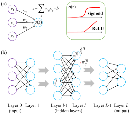
Figure 1: (a) Schematic representation of a neuron, the basic component of a neural network. The value of a neuron is determined by a linear transformation that weights the importance of various inputs, followed by a nonlinear activation function. Two typical nonlinear activation functions are also shown: sigmoid and ReLU. (b) Feed-forward neural network with neurons arranged into layers with the output of one layer serving as the input to the next layer.

A NN consists of many neurons stacked into layers, with the output of one layer serving as the input of the next one, see Fig. 1(b). In this simple feedforward fully-connected network, which is the architecture used throughout this work, the first layer ($l=0$) is called the input layer, the middle layers (from $l=1$ to $l=L-1$) are called hidden layers, and the final layer ($l=L$) is called the output layer. Here, we have $n_{l}$ neurons in layer $l$. The task of this network is for every input to produce an output, which will depend on the current value of the parameters of the model (weights and biases). To see how the network operates, let us consider a single input example with $n$ features encoded in the row vector $x=(x_{1},x_{2},\dots,x_{n})$. Let us call $W^{(l)}$ the $n_{l-1}\times n_{l}$ matrix whose element $W^{(l)}_{ij}$ is the weight connecting the neuron $i$ of layer $l-1$ with neuron $j$ of layer $l$, and $b^{(l)}$ the row vector whose element $b^{(l)}_{j}$ is the bias corresponding to neuron $j$ in layer $l$. The output of the network is obtained by going layer by layer, starting at the input layer $l=0$, whose neuron value is simply the example $x$ provided by the user, i.e.,

$$z^{(0)} = x,\;\;a^{(0)}=z^{(0)}$$

$$z^{(1)} = a^{(0)}W^{(1)}+b^{(1)},\;\;a^{(1)}=\sigma(z^{(1)})$$

$$\vdots$$

$$z^{(l)} = a^{(l-1)}W^{(l)}+b^{(l)},\;\;a^{(l)}=\sigma(z^{(l)})$$

$$\vdots$$

$$z^{(L)} = a^{(L-1)}W^{(L)}+b^{(L)},\;\;\hat{y}=a^{(L)}=\sigma(z^{(L)}).$$ (1)

Here, $z^{(l)}$ and $a^{(l)}$ are row vectors with $n_{l}$ elements and $\hat{y}$ is a row vector with $n_{L}$ elements containing the output of the network corresponding to the input $x$. Moreover, $\sigma(z^{(l)})$ should be understood as the element-wise application of the activation function $\sigma$, which could be different in different layers. These equations can be trivially generalized to deal in parallel with an arbitrary number of input examples.

Once a network architecture is fixed, the next step is to train the NN, i.e., to adjust the parameters of the model (weights and biases) to reproduce the desired function. Like in all supervised learning procedures, one starts by providing a set of examples (or training set) $\{(x_{i},y_{i});i=1,\dots,m\}$, where $x_{i}$ contains the $n$ input variables or features of example $i$, and $y_{i}$ corresponds to the target variable or output of example $i$. In the problems addressed in the following sections, the features will be the geometrical parameters defining the investigated structures (thickness, size, filling factor, etc.) and the number of these input variables will set the number of neurons of the input layer ($n_{0}=n$). On the other hand, the target will correspond to a spectral function (like a spectral thermal conductance or a frequency-dependent emissivity) that will be calculated numerically using different computational methods. The number of neurons of the output layer $n_{L}$ will be equal to the number of frequency or wavelength points used to represent that spectral function, and the value of the output neurons will correspond to the prediction made by the NN for that function. To train the network one also needs an error function, also known as cost or loss function, that provides a metric of the deviation between the NN output and the function that it is trying to approximate. A typical choice, which we will frequently use, is the mean square error (MSE) given by

$$E(\theta)=\frac{1}{m}\sum^{m}_{i=1}(y_{i}-\hat{y}_{i}(\bm{\theta}))^{2},$$ (2)

where $\bm{\theta}$ represents the set of model parameters (weights and biases), $m$ is the number of examples in the training set, $y_{i}$ is target $i$ and $\hat{y}_{i}$ is the NN prediction for example $i$.

Once the cost function has been defined, the idea is to find its minimum in the high-dimensional space of parameters $\bm{\theta}$. This minimization can be done with the method of gradient descent, or any of its generalizations [8], and a proper choice of the learning rate (the parameter that determines how big a step we should take in the direction of the gradient). In this work we have always made use of the ADAM optimizer [37], which has been shown to be a robust choice for deep learning optimization in a variety of different contexts [38]. ADAM makes use of running averages of both the gradients of the cost function and their second moments. In general, we have used ADAM as a stochastic algorithm. Stochasticity is incorporated by approximating the gradient of the cost function on a subset of the data called a minibatch, which has a size ($m_{\rm batch}$) much smaller than the number of training examples $m$. In every optimization step we use the mini-batch approximation to the gradient to update the parameters $\bm{\theta}$ and then we cycle over all $m/m_{\rm batch}$ minibatches one at a time. A full iteration over all $m$ data points (i.e., using all $m/m_{\rm batch}$ minibatches) is called an epoch.

Due to the large number of parameters $\bm{\theta}$, the training procedure of a NN requires a specialized algorithm, which is referred to as backpropagation [39, 40]. This algorithm is conceptually very simple and makes a clever use of the chain rule for derivatives of a multivariate function to compute the gradient of the cost function with respect to all the parameters in only one backward pass from the output layer to the input layer. This algorithm is described in many textbooks and reviews, see e.g. Refs. [40, 8, 10], and we have made use of it in all our calculations.

Another point worth mentioning is that, following the common practice in supervised learning, and in order to evaluate the ability of our models to generalize to previously not seen data, we have divided our training sets into two portions, the dataset we train on, which we shall simply refer to as training set, and a smaller validation (or cross-validation) set that allows us to gauge the out-of-sample performance of the model. While training our models, we have followed both the training error and the validation error (using the same cost function). Then, we have adjusted the hyperparameters, such as the number of layers and neurons per layer, to reduce the validation error to optimize the performance for a specific dataset. Additionally, one should also use a third and independent portion of the original dataset as test set, i.e., as a set that is neither used for training nor for validation and that provides an unbiased measure of the generalization ability of a model. This test set is strictly necessary when one uses any regularization method based on the validation error such as the so-called early stopping, otherwise the validation set plays very much the role of the test set and this latter one becomes unnecessary. Finally, we point out that most of our NN calculations were done using the open source library Tensorflow [41], and in particular, its higher level application programming interface (API) Keras [42].

III Near-field radiative heat transfer between multilayer systems

One of the major advances in recent years in the field of thermal radiation has been the experimental confirmation of the long-standing prediction that the limit set by Stefan-Boltzmann’s law for the radiative heat transfer between two bodies can be largely overcome by bringing them sufficiently close [43]. This phenomenon is possible because in the near-field regime, i.e., when the separation between two bodies is smaller than the thermal wavelength $\lambda_{\rm Th}$ ($\sim$10 $\mu$m at room temperature), radiative heat can also be transferred via evanescent waves (or photon tunneling). This mechanism provides an additional contribution not taken into account in Stefan-Boltzmann’s law and it turns out to dominate the near-field radiative heat transfer (NFRHT) for sufficiently small gaps o separations. Up to date, this phenomenon has been confirmed in numerous experiments and it has led to a huge experimental and theoretical activity on the topic of NFRHT, for recent reviews see Refs. [31, 29, 32]. The workhorse geometry in the study of NFRHT is that of two parallel plates and to maximize the heat transfer special attention has been devoted to the use of materials that exhibit electromagnetic surface modes at the body-vacuum interfaces, such as polar dielectrics (SiO₂, SiN, etc.) or metallic materials exhibiting surface plasmon polaritons in the infrared. Different strategies have been recently proposed to further enhance NFRHT [31, 29, 32]. One of the most popular ideas is based on the use of multiple surface modes that can naturally appear in multilayer structures. In this regard, a lot of attention has been devoted to multilayer systems where dielectric and metallic layers are alternated to give rise to hyperbolic metamaterials [44, 45, 46, 47, 48, 49, 50, 51, 52, 53]. The hybridization of surface modes appearing in different metal-dielectric interfaces have indeed been shown to lead to a great enhancement of the NFRHT, as compared to the case of two infinite parallel plates, see e.g. Ref. [51]. The goal of this Section is to show how NNs can be used to describe the NFRHT between multilayer structures and how they can assist in the design and optimization of these structures for different purposes.

Following Ref. [51], we consider here the radiative heat transfer between two identical multilayer structures separated by a gap $d_{0}$, as shown in Fig. 2(a). Each body contains $N$ total layers alternating between a metallic layer with a permittivity $\epsilon_{\mathrm{m}}$ and a lossless dielectric layer of permittivity $\epsilon_{\mathrm{d}}$. The thickness of the layer $i$ is denoted by $d_{i}$ and it can take any value within a given range (to be specified below). While the dielectric layers will be set to vacuum ($\epsilon_{\mathrm{d}}=1$), the metallic layers will be described by a permittivity given by a Drude model:

$$\epsilon_{\mathrm{m}}(\omega)=\epsilon_{\infty}-\frac{\omega^{2}_{p}}{\omega(\omega+i\gamma)},$$ (3)

where $\epsilon_{\infty}$ is the permittivity at infinite frequency, $\omega_{p}$ is the plasma frequency, and $\gamma$ de damping rate. From now on, we set $\epsilon_{\infty}=1$, $\omega_{p}=2.5\times 10^{14}$ rad/s, and $\gamma=1\times 10^{12}$ rad/s.

We describe the radiative heat transfer within the framework of theory of fluctuational electrodynamics [54, 55] and focus on the near-field regime. In this regime, the radiative heat transfer is dominated by TM- or $p$-polarized evanescent waves and the heat transfer coefficient (HTC) between the two bodies, i.e., the linear radiative thermal conductance per unit of area, is given by [30]

$$h=\frac{\partial}{\partial T}\int^{\infty}_{0}\frac{d\omega}{2\pi}\Theta(\omega,T)\int^{\infty}_{\omega/c}\frac{dk}{2\pi}\,k\tau_{p}(\omega,k),$$ (4)

where $T$ is temperature, $\Theta(\omega,T)=\hbar\omega/(e^{\hbar\omega/k_{\rm B}T}-1)$ is the mean thermal energy of a mode of frequency $\omega$, $k$ is the magnitude of the wave vector parallel to the surface planes, and $\tau_{p}(\omega,k)$ is the transmission (between 0 and 1) of the $p$-polarized evanescent modes given by

$$\tau_{p}(\omega,k)=\frac{4\left[\mbox{Im}\left\{r_{p}(\omega,k)\right\}\right]^{2}e^{-2q_{0}d_{0}}}{|1-r_{p}(\omega,k)^{2}e^{-2q_{0}d_{0}}|^{2}}.$$ (5)

Here, $r_{p}(\omega,k)$ is the Fresnel reflection coefficient of the $p$-polarized evanescent waves from the vacuum to one of the bodies and $q_{0}=\sqrt{k^{2}-\omega^{2}/c^{2}}$ ($\omega/c<k$) is the wave number component normal to the layers in vacuum. The Fresnel coefficient needs to be computed numerically and we have done it by using the scattering matrix method described in Ref. [56]. In our numerical calculations of the HTC we also took into account the contribution of $s$-polarized modes, but it turns out to be negligible for the gap sizes explored in this work.

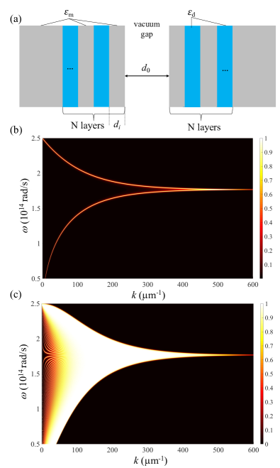
Figure 2: (a) Sketch of two identical multilayer systems separated by a vacuum gap of size $d_{0}$. The two reservoirs feature $N$ total layers alternating between a Drude metal (grey areas) with permittivity $\epsilon_{\mathrm{m}}$ and a dielectric (white areas) with permittivity $\epsilon_{\mathrm{d}}$. The last layer in both cases is made of metal and the thickness of layer $i$ is denoted by $d_{i}$. (b) The transmission of the evanescent waves as a function of the frequency $\omega$ and the magnitude of the parallel wave vector $k$ for the bulk system, i.e., two parallel plates made of the metal, and $d_{0}=10$ nm. (c) The same as in panel (b), but for the multilayer system with $N=160$ and $d_{i}=10$ nm for all layers.

Let us briefly recall that, as explained in Ref. [51], the interest in the NFRHT in this multilayer structures resides in the fact that the heat exchange in this regime is dominated by surfaces modes that can be shaped by playing with the layer thicknesses. In the case of two parallel plates made of a Drude metal, the NFRHT is dominated by the two cavity surface modes resulting from the hybridization of the surface plasmon polaritons (SPPs) of the two metal-vacuum interfaces [51]. As shown in Fig. 2(b), these two cavity modes give rise to two near-unity lines in the transmission function $\tau_{p}(\omega,k)$. Upon introducing more internal layers with appropriate thickness, one can have NFRHT contributions from surface states at multiple surfaces, as we illustrate in Fig. 2(c) for the case of $N=160$ layers. As shown in Ref. [51], the contribution of these additional surface states originating from internal layers can lead to a great enhancement of the NFRHT as compared to the bulk system (two parallel plates) in a wide range of gap values. Our goal in this Section is to show that NNs can learn the NFRHT characteristics of these multilayer systems and that they can be used in turn to solve inverse design and optimization problems in this context.

We start by considering the NFRHT between two systems formed by $N=4$ layer (2 metallic and 2 dielectric layers). We set the vacuum gap to $d_{0}=10$ nm and the temperature to $T=300$ K. Our objective is to show that a NN can learn, in particular, the spectral HTC $h_{\omega}$, i.e., the HTC per unit of frequency: $h=\int^{\infty}_{0}h_{\omega}d\omega$. To train the network, we used the theory detailed above and prepared a training set with 881 $h_{\omega}$-spectra where the thicknesses $d_{i}$ of the 4 layers were varied between 5 and 20 nm. Every spectrum contains 200 frequency points in the range $\omega\in[0.3,3]\times 10^{14}$ rad/s. The training set was, in turn, divided into 80% for actual training and 20% for the test set. In this case we found that a NN with 5 hidden layers and 250 neurons per layer was able to accurately reproduce the training set. This network contains 4 neurons in the input layer (corresponding to the 4 input parameters, i.e., the layer thicknesses), while the output layer has 200 neurons corresponding to the frequency values in the $h_{\omega}$-spectra. The NN was trained during 50,000 epochs using the MSE as the cost function, the ADAM optimizer, the ReLU activation function in all layers, except in the output one, and we did not use early stopping. We found helpful to use a variable learning rate ($l_{r}$) to improve the training given by $l_{r}=0.001\times 0.3^{p/20,000}$, where $p$ is the number of epochs (the numerical values defining $l_{r}$ have been found by a trial-and-error process). To give a quantitative idea about the ability of our network to reproduce the training set and to generalize, we calculated the average relative error in the integral of the $h_{\omega}$-spectra (i.e., the total HTC) and found that is 0.81% for the training set and 1.45% for the test set. The generalization accuracy of the NN is illustrated in Fig. 3(a) where we show how the network is able to reproduce different spectra from the test set (i.e., spectra it was not trained on).

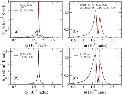
Figure 3: Results for the spectral heat transfer coefficient $h_{\omega}$ between two multilayers with $N=4$ and a gap size $d_{0}=10$ nm. (a) Comparison between real $h_{\omega}$-spectra computed with fluctuational electrodynamics (solid lines) and the prediction of the NN (dashed lines). The layer thicknesses (in nm) are indicated in the legend. (b) Comparison of the NN approximation to the target spectrum (layer thicknesses in nm are indicated in the legend) following the inverse design problem described in the text. (c) Result of the optimization problem in which the total heat transfer coefficient is maximized. (d) Result of the optimization problem where $h_{\omega}$ is minimized in the frequency region indicated by the dashed vertical lines.

As a next step, we show how the NN can be used to solve inverse design problems. As proof-of-principle calculation, the idea is to show that with the help of the NN we can find the layer thicknesses that would be able to reproduce an arbitrary $h_{\omega}$-spectrum. For this purpose, we freeze all the parameters of the NN and use backpropagation to train the inputs. This is done by fixing the output to the desired output and iterating the input to minimize the difference between the spectrum predicted by the NN and the target spectrum. This means in practice that the cost function for this task is simply defined as the MSE between the predicted and the target spectrum. This minimization process is very efficient because the gradients of the cost function with respect to the inputs can be computed analytically using backpropagation [18]. Once the minimization process is finished, the NN suggests the thickness values to reproduce the target spectrum. We illustrate this inverse design problem in Fig. 3(b) where the target spectrum was randomly chosen to correspond to the layer thicknesses $\{d_{1},d_{2},d_{3},d_{4}\}=\{5.0,12.5,12.5,16.25\}$ nm (to ensure that we have a physically realizable spectrum). Notice that the NN is able to reproduce this target spectrum very well and suggests that the corresponding layer thicknesses are $\{5.0,12.45,12.66,16.55\}$ nm, which is in excellent agreement with the actual value.

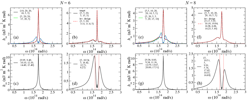
Figure 4: (a-d) Same as in Fig. 3 but now for $N=6$. (e-h) Same as in Fig. 3 but for $N=8$.

We now want to illustrate how the NN can also be used to solve optimization problems. A first natural problem is to determine the layer structure (with $N=4$) that maximizes the total HTC $h$. Naively, in the limit $N\to\infty$ one expects to maximize the HTC by having all the layer thicknesses equal and equal to the gap size ($d_{0}=10$ nm) [51], but for finite $N$ this is not necessarily the case and one cannot simply rely on physical intuition. This optimization problem can be easily solved by fixing the parameters of the NN, using the total HTC as the cost function to be maximized, and optimizing the network with respect to the input parameters (layer thicknesses). The result for this optimization problem is shown in Fig. 3(c) and the optimal thicknesses are $\{9.29,9.78,11.84,14.43\}$ nm that lead to a total HTC at room temperature of $1.01\times 10^{5}$ W/(m²K). This value is $\sim 2.9$ larger than the HTC of the bulk system [$0.35\times 10^{5}$ W/(m²K)], which illustrates the fact that these multilayer systems can be used to further increase the NFRHT. Notice also that the optimal result is close to the case where all $d_{i}$ are equal to the value of the gap size ($d_{0}$), which as mentioned above would the naive choice based on the idea of a quasi-periodic system, which in turn would reduce the (Anderson-like) disorder in the structure.

Another interesting optimization problem consists in minimizing the heat transfer in a given frequency region, see Fig. 3(d), which might be motivated by the desire to inhibit the heat transfer in a certain frequency range. In this case, the cost function is defined as the ratio of the average of $h_{\omega}$ inside the range of interest and the corresponding average outside that region: $E=\bar{h}_{\omega,\mathrm{in}}/\bar{h}_{\omega,\mathrm{out}}$. The result of this optimization problem is shown in Fig. 3(d) and the corresponding layer thicknesses are $\{5.0,12.44,5.0,19.32\}$ nm. Notice that the network suggests rather disparate thicknesses for the neighboring layers and, in particular, the smallest possible thickness (within the range explored here) for the first metallic layer. This latter fact simply means that it is advantageous to have the first metallic layer as thin as possible to make it transparent and avoid the contribution of the surface mode appearing in the layer 1-vacuum interface at $\omega_{p}/\sqrt{2}\approx 1.77\times 10^{14}$ rad/s, which corresponds to the center of the chosen gap.

We extended our analysis above to structures with 6 and 8 layers. As explained above, the presence of additional layers in the system makes possible to the appearance of extra surface states that may lead to the increase in the heat transfer [51]. On the other hand, from a deep learning standpoint, the additional degrees of freedom associated to the additional layers enables the used NNs to feature broader generalization abilities. For this purpose, we used the same network architecture (only changing the number of features in the input layer) and studied the same inverse and optimization problems. The results for these two structures are summarized in Fig. 4. The NNs were trained in these two cases with training sets containing 4825 $h_{\omega}$-spectra for $N=6$ and 65536 for $N=8$. Again, this amounts to an average of 4-5 thickness values per layer in the same range as for $N=4$. The training was done using the same cost function, optimizer, variable learning rate scheme, and the same division (80%-20%) between training and test set. The main difference in the training was the use of transfer learning, a standard technique in deep learning which consists in using the parameters (weights and biases) of certain layers of a pre-trained network to train another network with similar architecture. In our case, we found that the best strategy is to use the parameters of all the layers of the network for $N=4$ ($N=6$) to initialize the parameters of the network for $N=6$ ($N=8$) and then proceed with the training. Since the networks for different values of $N$ have different number of neurons in the input layer, the extra parameters in the first layer were initialized randomly. With the help of transfer learning, we achieved average relative errors in the total integral of the $h_{\omega}$-spectra of 1.28% (1.95%) for the training set and 1.70% (2.00%) for the structure with $N=6$ ($N=8$). Without transfer learning the corresponding errors were 1.52% (2.81%) for the training set and 1.81% (2.83%) for the structure with $N=6$ ($N=8$), which is a significant difference.

Another important point to highlight is that in the optimization problem, which consists in maximizing the total heat transfer resulted in an optimal structure for $N=6$ with thicknesses $\{9.95,9.49,10.10,12.10,14.49,15.49\}$ nm with a HTC of $1.19\times 10^{5}$ W/(m²K), while for $N=8$ the optimal structure is $\{9.36,8.80,9.34,11.18,12.59,13.67,20.00,17.51\}$ nm with a HTC of $1.31\times 10^{5}$ W/(m²K). Notice that, as expected, the maximum HTC increases with the number of layers in the structure.

Let us conclude this Section by emphasizing that the study presented here can be extended to essentially any multilayer system, which may include anisotropic materials and metamaterials, in general, or the effect of external fields [57, 53]. Moreover, it could also be straightforwardly extended to deal with NFRHT between periodically patterned structures [58] (this is exemplified in the following Section in the case of far-field emission).

IV Passive radiative cooling

Recently it has been shown that it is possible to cool down a device by simply exposing it to sunlight and without any electricity input [59, 60]. This striking phenomenon, referred to as passive radiative cooling, is possible due to the fact that the Earth’s atmosphere has a transparency window for electromagnetic radiation between 8 and 13 $\mu$m that coincides with the peak thermal radiation wavelengths at typical ambient temperatures. By exploiting this window one can cool a body on the Earth’s surface by radiating its heat away into the cold outer space. While nighttime radiative cooling has been widely studied in the past, the first proposal to realize this phenomenon during daytime was put forward in 2013 by Rephaeli et al. [59]. Inspired by nanophotonic concepts, these authors proposed a passive cooler that consisted of two thermally emitting photonic crystal layers comprised of SiC and quartz, with a broadband solar reflector underneath. Subsequently, the same group designed and fabricated a multilayer photonic structure consisting of seven dielectric layers deposited on top of a silver mirror [60]. This design was shown to reach a temperature that is 5^oC below the ambient air temperature, in spite of having about 900 W/m² of sunlight directly impinging upon it. After this first realization, there has been an intense research activity with the goal to optimize this daytime radiative cooling [61, 62, 63, 64, 65, 66, 67, 68, 69, 70, 71, 72]. The goal of this Section is to illustrate how deep learning techniques can help in the theoretical design of devices for passive radiative cooling.

Let us start by recalling the basics of the theory of passive radiative cooling following Refs. [59, 60]. Consider a radiative cooler of area $A$ at temperature $T$, whose spectral and angular emissivity is $\varepsilon(\lambda,\theta)$. When the radiative cooler is exposed to a daylight sky, it is subject to both solar irradiance and atmospheric thermal radiation (corresponding to an ambient air temperature $T_{\rm amb}$). The net cooling power $P_{\rm cool}$ of such a radiative cooler is given by the following power balance:

$$P_{\rm cool}=P_{\rm rad}(T)-P_{\rm atm}(T_{\rm amb})-P_{\rm Sun}-P_{\rm cond+conv}.$$ (6)

Here, $P_{\rm rad}$ corresponds to the power radiated out by the structure and it is given by

$$P_{\rm rad}(T)=A\int d\Omega\cos\theta\int^{\infty}_{0}d\lambda\,I_{\rm BB}(\lambda,T)\varepsilon(\lambda,\theta),$$ (7)

where $\int d\Omega=2\pi\int^{\pi/2}_{0}d\theta\sin\theta$ is the angular integral over a hemisphere and

$$I_{\rm BB}(\lambda,T)=\frac{2hc^{2}}{\lambda^{5}}\frac{1}{e^{hc/(\lambda k_{\rm B}T)}-1}$$ (8)

is Planck’s distribution describing the spectral radiance of a blackbody at temperature $T$. On the other hand, $P_{\rm atm}$ is the absorbed power due to incident atmospheric thermal radiation and it is given by

$$P_{\rm atm}(T_{\rm amb})=A\int d\Omega\cos\theta\int^{\infty}_{0}d\lambda\,I_{\rm BB}(\lambda,T_{\rm amb})\times\\ \varepsilon(\lambda,\theta)\varepsilon_{\rm atm}(\lambda,\theta),$$ (9)

where $T_{\rm amb}$ is the ambient atmospheric temperature and $\varepsilon_{\rm atm}(\lambda,\theta)$ is the angle-dependent emissivity of the atmosphere [73]. The term $P_{\rm Sun}$ in Eq. (6) is the incident solar power absorbed by the structure and is given by

$$P_{\rm Sun}=A\cos(\theta_{\rm Sun})\int^{\infty}_{0}d\lambda\,I_{\rm AM1.5}(\lambda)\varepsilon(\lambda,\theta_{\rm Sun}),$$ (10)

where $I_{\rm AM1.5}(\lambda)$ is the AM1.5 spectrum representing the solar illumination and $\theta_{\rm Sun}$ corresponds to the angle at which the structure is facing the Sun, which we shall assume to be zero. Finally, the term $P_{\rm cond+conv}$ in Eq. (6) is the power lost due to convection and conduction and adopts the form

$$P_{\rm cond+conv}(T,T_{\rm amb})=A\>h_{c}\>(T_{\rm amb}-T),$$ (11)

where $h_{c}=h_{\rm cond}+h_{\rm conv}$ is a combined non-radiative heat coefficient that takes into account the net effect of conductive and convective heating due to the contact of the cooler with external surfaces and the air adjacent to the radiative cooler.

A given structure behaves effectively as a daytime cooling device when $P_{\rm cool}>0$ at the ambient temperature, i.e., when the power radiated out by the cooler is greater than the combined effects of the incoming sources of heat from the Sun, atmosphere, and local conduction/convection. The power outflow $P_{\rm cool}(T=T_{\rm amb})$ then defines the device’s cooling power at ambient air temperature. Another important metric of the performance of the device is the equilibrium temperature, $T_{\rm eq}$, at which $P_{\rm cool}=0$ in Eq. (6). A radiative cooler with $T_{\rm eq}$ below the ambient temperature would cool an attached structure to a temperature below ambient over time.

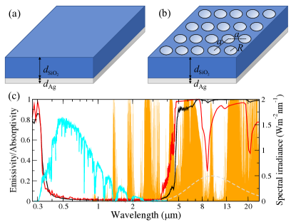
Figure 5: (a) Schematics of the silica mirror used as a passive radiative cooler in Ref. [64]. It consists of a SiO₂ slab of thickness $d_{\mathrm{SiO_{2}}}$ and a silver thin film of thickness $d_{\mathrm{Ag}}$. (b) A nanostructured version of the cooler of panel (a), but featuring a periodic array of circular holes of radius $R$ with a lattice parameter $a$ (square lattice). (c) Emissivity as a function of the wavelength for a silica photonic crystal (black solid line) and a silica mirror (red solid line) for $d_{\mathrm{SiO_{2}}}=500$ $\mu$m and $d_{\mathrm{Ag}}=120$ nm. For the photonic crystal: $a=100$ nm and $R=50$ nm ($f=0.785$). The cyan solid line corresponds to the AM1.5 solar spectrum $I_{\rm AM1.5}$ (see right vertical axis), the orange curve to the atmospheric emissivity/absorptivity spectrum $\varepsilon_{\rm atm}$, and the gray dashed line to the blackbody radiation curve $I_{\rm BB}$ (50 times enlarged in spectral irradiance) at 300 K.

From the discussion above, it is obvious that the basic requirements for a structure to be a good passive cooler are: (i) to selectively emit thermal radiation in the atmospheric transparency window (from 8 to 13 $\mu$m), and, (ii) to reflect the solar radiation as much as possible. This requires to tune the emissivity over a very wide range (from the mid-infrared to the ultraviolet) and many complex structures have been proposed and realized. Here, we shall use as a starting point a rather simple configuration put forward in Ref. [64], which consists of a silica mirror, see Fig. 5(a), featuring a SiO₂ slab of thickness $d_{\mathrm{SiO_{2}}}$, which is responsible of a near-ideal blackbody in the mid-infrared, and a silver thin film of thickness $d_{\mathrm{Ag}}$, which provides reflection for the solar radiation. This simple structure with $d_{\mathrm{SiO_{2}}}=500$ $\mu$m and $d_{\mathrm{Ag}}=120$ nm was shown to achieve radiative cooling below ambient air temperature under direct sunlight ($\sim 8$^oC), which clearly outperforms more sophisticated designs [60]. Furthermore, it was estimated that this cooler reached an average net cooling power of $\sim 110$ W/m² during daytime at ambient temperature even considering the significant influence of external conduction and convection [64]. The device’s performance was also shown to slightly improve by coating it with a polymer. In what follows, we shall investigate how the performance of this silica mirror can be improved via nanostructuration and how NNs can used to optimize its design.

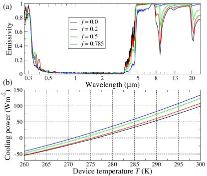
Figure 6: (a) Emissivity of the photonic crystal cooling device as a function of the wavelength for several filling factors $f$ and a hole radius $R=50$ nm. The rest of the parameters are: $d_{\mathrm{SiO_{2}}}=500$ $\mu$m and $d_{\mathrm{Ag}}=120$ nm. (b) The corresponding cooling power density as a function of the device temperature under AM1.5 illumination. The ambient temperature of the atmosphere is taken to be $T_{\mathrm{amb}}=300$ K.

To be precise, we shall now discuss how the introduction of a periodic array of air circular holes in the silica layer can boost the performance of the device as a passive cooler, see Fig. 5(b). We consider the case of a square lattice with a lattice parameter $a$ and holes of radius $R$. We define the filling factor $f$ as the fraction of the area occupied by the air holes: $f=\pi(R/a)^{2}$, which varies between 0 (no holes) and $\pi/4\approx 0.785$ (for the largest possible holes, $R=a/2$). The basic idea is that this photonic crystal can enhance the emissivity of silica in the atmospheric transparency window, while maintaining the sunlight absorption of the unstructured silica mirror [74]. The infrared enhancement of the photonic crystal is simply due to a reduction of the impedance mismatch between the silica surface and the surrounding air. This effect is illustrated in Fig. 5(c) where we compare the normal-incidence emissivity of a silica photonic crystal with the corresponding silica mirror with no holes. For reference, we also show in that figure the AM1.5 spectrum, the normal-incidence of the atmosphere’s emissivity and Planck’s blackbody distribution. As one can see, the photonic crystal device behaves almost as a black body in the relevant infrared region, which is precisely what we are looking for.

We illustrate in more detail the role of the nanostructuration in Fig. 6(a) where we show how the emissivity of a photonic crystal device progressively increases in the atmospheric transparency window upon increasing the filling factor. In this example we set $R=50$ nm, $d_{\mathrm{SiO_{2}}}=500$ $\mu$m, and an ambient temperature $T_{\mathrm{amb}}=300$ K. The emissivity increase in the mid-infrared results in an improvement of the performance of the cooling device as shown in Fig. 6(b) where we display the corresponding cooling power $P_{\mathrm{cool}}$ as a function of the device temperature $T$. Here, we have ignored the contribution of non-radiative processes (conduction and convection) and approximated the emissivities by the normal incidence results (this approximation will be used throughout this Section). Notice that upon increasing the filling factor, the cooling power can increase up to a 40% at ambient temperature (300 K) and the equilibrium temperature $T_{\mathrm{eq}}$ can be reduced by $\sim 5$^oC, as compared to the unstructured silica mirror.

All the results in this work for the emissivity of the periodically patterned structures were calculated using the rigorous coupled wave analysis (RCWA) described in Ref. [56]. It is important to stress that this is a numerically exact method that makes use of the so-called fast Fourier factorization when dealing with the Fourier transform of two discontinuous functions in the Maxwell equations. This factorization solves the known convergence problems of the RCWA approach, see Ref. [56] for details, and its use was critical in this case because we deal with materials with very different dielectric functions and the emissivities have to be computed over a huge wavelength range (from the UV to the mid-infrared). Owing to its ability to generate training sets in a robust and efficient way, our own implementation of the RCWA method became a key ingredient in the successful application of deep techniques in this context.

Finally, we point out that for all the parameter values considered here, we made sure that the emissivity spectra were converged up to a 1% relative error for every wavelength point. This required to take into account up to several thousand plane waves for the shortest wavelength (UV/visible range) and the largest holes. To give an idea of the required computational time, the most time-consuming emissivity spectra took about 24 hours in a desktop computer with a 2.3-GHz Intel Xenon processor running in parallel in 18 CPUs. For the RCWA calculations we used as an input the dielectric function of SiO₂ tabulated in Ref. [75] and for Ag that of Ref. [76].

To study systematically the role of the nanostructuration in the performance of the cooler, we define the following optimization problem. We consider as input parameters the silica layer thickness $d_{\mathrm{SiO_{2}}}$, the filling factor $f$, and the hole radius $R$ (we fix the thickness of the back reflector to $d_{\mathrm{Ag}}=120$ nm), and we search for the optimal values of these parameters to maximize the cooling power at ambient temperature. To solve this problem with the help of NNs, we first constructed a training set with RCWA calculations of the emissivity of the cooler, which were then used to compute $P_{\mathrm{cool}}$ using Eqs. (6)-(11). The training set contained 900 emissivity spectra with 15 different values of $d_{\mathrm{SiO_{2}}}$ between 1 and 2000 $\mu$m, 10 different values of $f$ between 0 and $\pi/4$, and 6 values of $d_{\mathrm{SiO_{2}}}$ from 30 to 200 nm. Every spectrum contains the emissivity for 525 wavelength values ranging from 270 nm to 25 $\mu$m. A preliminary analysis using this training set indicated that below hole radii of 100 nm the results are fairly insensitive to the exact radius value, while for larger holes the sunlight absorption increases and the performance of the device decreases drastically. For this reason, we fixed the radius value to $R=30$ nm, and reduced the input parameters to $d_{\mathrm{SiO_{2}}}$ and $f$ (the filling factor). Thus, our training set contained in practice 150 emissivity spectra, which were divided into an actual training set (80%) and a test set (20%).

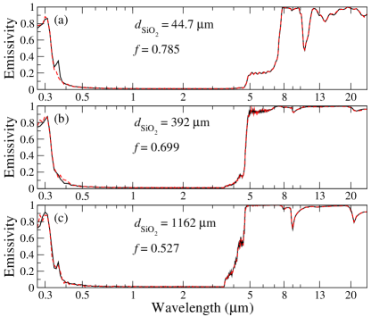
Figure 7: (a-c) Comparison between the emissivity spectra of silica photonic crystal devices computed with the RCWA method (solid lines) and the prediction of the NN (dashed lines) for different values of the silica layer thickness and filling factor, as indicated in the legends. The hole radius is $R=30$ nm and $d_{\mathrm{Ag}}=120$ nm.

For this problem we found that a NN with 3 hidden layers (with 250 neurons per layer) is enough to satisfactorily reproduce the training set. This network contains two neurons in the input layer (corresponding to the two input parameters or features in this problem), while the output layer has 525 neurons corresponding to the wavelength values in the emissivity spectra. The NN was trained during 50,000 epochs using the MSE as the cost function, the ADAM optimizer, and the ReLU activation function in all layers, except in the output one. No early stopping was used in this case. After training, the MSE for the training set was $4.6\times 10^{-5}$ and $4.4\times 10^{-4}$ for the test set. In Fig. 7 we illustrate the ability of this NN to reproduce emissivity spectra of the test set. As seen, the NN is able to accurately reproduce very different spectra over the entire wavelength range, which demonstrates the ability of our NN to generalize to cases it was not trained on. It is also remarkable to find that degree of accuracy despite the moderate size of our training set (as mentioned, formed by just 150 samples).

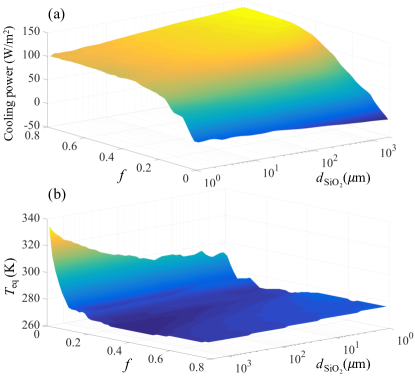
Figure 8: (a) Cooling power density as a function of the silica thickness layer and filling factor of photonic crystal cooling devices as computed with the trained NN. In this case, the device temperature and the ambient temperature were assumed to be 300 K. The contribution of non-radiative processes was neglected. (b) The corresponding equilibrium temperature.

Next, we used the NN as a computational engine to solve our optimization problem, namely the maximization of the device’s cooling power. As explained in the previous Section, this optimization process is very efficient because we can analytically compute the NN gradients with respect to the inputs using backpropagation [18]. In Fig. 8(a) we illustrate the results predicted by the NN for the cooling power density as a function of the filling factor and the silica layer thickness for $T=T_{\mathrm{amb}}=300$ K. For these calculations, and since we are mainly interested in comparing with the results for the unstructured silica mirror, we ignored the contribution of the non-radiative processes (conduction and convection). For completeness, we also show in Fig. 8(b) the corresponding equilibrium temperature. Let us remind that, contrary to the cooling power, the equilibrium temperature is very sensitive to the contribution of conduction and convection. As it is obvious from Fig. 8(a), the optimization process suggests that the optimal parameters are $f=0.785$ and $d_{\mathrm{SiO_{2}}}=2$ mm. This means that the filling factor has to be as large as possible, which confirms the naive expectation. With respect to the silica layer thickness, there is no significant difference in the cooling power in the range $d_{\mathrm{SiO_{2}}}\in[500\,\mu\mbox{m},2\,\mbox{mm}]$.

The study presented in this Section can be generalized in a number of ways. For instance, we also analyzed the role of a finite depth of the air holes (in the calculations discussed above, it was assumed that the silica layer was perforated all the way down to the Ag thin film). In particular, we found that for the optimal parameters found above, a hole depth of around 10 $\mu$m is enough to reach values for the cooling power very similar to those obtained for a fully perforated silica layer. Of course, there are a number of different Bravais lattices that one could also explore, as well as many different shapes of the air holes. In the case of regular hole shapes one could still use sequential fully connected NNs like in this work, but if one wants to consider arbitrary shapes it might be more convenient to use two-dimensional convolutional neural networks (CNNs) [77], which have already been successfully used in the context of nanophotonics for the design of metasurfaces with desired properties [12, 13, 14, 15, 16, 17].

V Thermal emission of subwavelength objects

The goal of this Section is to show how NNs can also be helpful in the context of the description of the thermal emission of a single object of arbitrary size and shape. In particular, we are interested in the thermal emission of subwavelength objects, i.e., objects in which some of their dimensions are smaller than the thermal wavelength $\lambda_{\rm Th}$. Part of the interest in this problem lies in the fact that, as already acknowledged by Planck in his seminal work [78], Planck’s law fails to describe the thermal properties of subwavelength objects simply because it is based on ray optics. In this sense, one may wonder whether the blackbody limit for the thermal emission of a body (given by Stefan-Boltzmann’s law) can be overcome in the case of subwavelength objects, something that is not possible in the case of infinite objects. Actually, it is well-known that the emissivity of a finite object can be greater than 1 at certain frequencies [79, 80], but that is not enough to emit more than a black body. In fact, only a modest super-Planckian thermal emission has been predicted in rather academic situations [81, 82], and it has never been observed. Recently, Fernández-Hurtado et al. [83] showed that elongated objects with subwavelength dimensions can indeed have directional emissivities much larger than 1, which can lead to super-Planckian far-field radiative heat transfer between two of those bodies, as it has been experimentally verified [84]. However, the total thermal emission of those objects is still smaller than that of a black body. There are by now several experiments showing the failure of Planck’s law in the description of the thermal emission of subwavelength objects (although no super-Planckian emission has yet been observed). For instance, Ref. [85] reported this failure in the case of small optical fibers, while Ref. [86] did it in the case of nanoribbons made of silica with a thickness of 100 nm, much smaller than both $\lambda_{\rm Th}$ and the skin depth, while the other dimensions could be much larger. From the theory side, the description of the thermal emission of a single object of arbitrary size and shape continues to be very challenging and there is only a handful of general-purpose numerical approaches that can tackle this problem [87, 88, 89, 90, 91]. These techniques are often exceedingly time consuming and systems like the nanoribbons explored in Ref. [86] are still out of the scope of these techniques. Thus, in the rest of this Section we shall show how the use of NNs can contribute to alleviate this situation.

The total power emitted by any object at a temperature $T$ is given by [26]

$$P_{\rm em}=\pi A\int^{\infty}_{0}d\omega\,I_{\rm BB}(\omega,T)\varepsilon(\omega),$$ (12)

where $A$ is the total area of the object, $\varepsilon(\omega)$ is the angular-averaged frequency-dependent emissivity of the body, and $I_{\rm BB}(\omega,T)$ is the frequency-dependent Planck distribution given by

$$I_{\rm BB}(\omega,T)=\frac{\omega^{2}}{4\pi^{3}c^{2}}\frac{\hbar\omega}{e^{\hbar\omega/k_{\rm B}T}-1}.$$ (13)

In the case of a black body, $\varepsilon(\omega)=1$ for all frequencies and the total emitted power is given by Stefan-Boltzmann law: $P_{\rm em,BB}=A\sigma T^{4}$, where $\sigma=5.67\times 10^{-8}$ W/(m²K⁴).

To illustrate the use of NNs in this particular context, we consider here a proof-of-principle example, namely the thermal emission of a silica cube of arbitrary side $L$ and at room temperature ($T=300$ K), see inset of Fig. 9(b). A cube is already a sufficiently complicated geometry such that its emissivity cannot be calculated analytically. We have computed this emissivity using the numerical approach known as thermal discrete dipole approximation (TDDA), as described in section IV of Ref. [91]. In this approach, an object is discretized in terms of point dipoles in the spirit of the DDA method that is widely used for describing the scattering and absorption of light by small particles [92, 93]. In our case, we modeled silica cubes with sides ranging from 0.1 $\mu$m (much smaller than the thermal wavelength) to 20 $\mu$m, which is comparable to the thermal wavelength. We discretized the cubes in terms of a lattice of cubic dipoles and used up to $\sim 12000$ dipoles, which was checked to be enough to accurately converge the results even for the largest cubes considered here. The calculation of a single spectrum with 200 frequency points and with a discretization with $\sim 12000$ dipoles took about 24 hours in a desktop computer with a 2.3-GHz Intel Xenon processor running in parallel in 18 CPUs. The dielectric function of SiO₂ was taken from the tabulated values in Ref. [75].

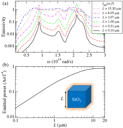
Figure 9: (a) Emissivity of a silica cube of side $L$ as a function of the frequency. The dotted orange line corresponds to Planck’s distribution $I_{\rm BB}(\omega,T)$ at $T=300$ K in arbitrary units. (b) Total power emitted by a SiO₂ cube (see inset) as a function of its side $L$ at $T=300$ K. The power is normalized with the blackbody result, $A\sigma T^{4}$, where $A=6L^{2}$ is the total area of the cube.

A representative set of examples of the computed emissivity are shown in Fig. 9(a) for various values of $L$. Notice that for certain frequencies the emissivity can be larger than 1 (e.g., for $L=1\,\mu$m and $\omega\sim 2.1\times 10^{14}$ rad/s, $\varepsilon\sim 2.9$). However, this does not mean that a silica cube can be a super-Planckian emitter. As we show in Fig. 9(b) where one can see the total emitted power as a function of $L$, a cube always emits less than a black-body cube of the same size. Notice also that for small cubes the emitted power is proportional to the cube volume, which is due to the fact that in this regime the silica skin depth at the relevant frequencies is larger than $L$ [94, 95]. This means that the whole object contributes to the thermal emission. However, as the size increases, the emitted power becomes proportional the cube area and it tends to converge to the value of an infinite silica surface, which with the optical constants used here is equal to 0.79 at room temperature. This behavior reflects the fact that when $L$ becomes larger than the skin depth, the thermal emission only originates from the surface, as it happens in macroscopic objects.

Now we show that a NN can learn the emissivity spectra of a cube. For this purpose, we have computed a training set of 100 emissivity spectra with $L\in[0.1\,\mu\mbox{m},20\,\mu\mbox{m}]$ with equally spaced side values in a logarithmic scale. Additionally, we have calculated another 20 spectra in the same range to form the test set. Later on we shall explore what happens when varying the size of the training set. In this case, we have done a hyperparameter search (changing the number of layers, the number of neurons per layer, the learning rate, etc.), and used $k$-fold cross-validation (with $k=5$) to select the optimal hyperparameters [96]. The only input feature in this was the cube side (i.e., we have a single neuron in the input layer), and the output was the emissivity spectrum sampled at 200 equidistant points between $0.15\times 10^{14}$ and $3.04\times 10^{14}$ rad/s (i.e., the output layer has 200 neurons). The NNs were trained using the MSE as the cost function, the ADAM optimizer, and the ReLU activation function in all layers, but the output one where no activation function was used as it is customary in a regression problem. The NNs were trained for a maximum of $\sim 50,000$ epochs and we used early stopping based on the validation error to conclude the training. We found that an optimal NN is composed of 4 hidden layers with 250 neurons per layer, which is the network we used for all the calculations that we are about to describe.

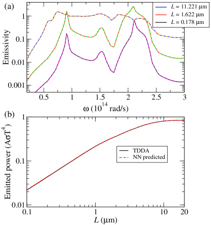
Figure 10: (a) Comparison between the real emissivity spectra of a SiO₂ cube computed with TDDA (solid lines) and the prediction of the NN (dashed lines) for various values of cube side $L$. (b) The corresponding comparison for the total power emitted by a SiO₂ cube as a function of its side $L$ at $T=300$ K. The power is normalized with the blackbody result.

As in the previous examples, the first application was to test the forward computation of the network to see how well it reproduces the emissivity spectra it was not trained on. This is illustrated in Fig. 10(a) where we show that the NN can very accurately reproduce several representative examples of the test set. We also show in Fig. 10(b) that using the NN predictions for the emissivity spectra and Eq. (12), we can accurately reproduce the size-dependence of the total emitted power. To be more quantitative, we computed the average relative error per point in the emissivity spectra and found that is equal to $0.65$% for the training set and $0.63$% for the test set, which demonstrates the excellent generalization ability of the optimal NN.

Now, we illustrate the possibility to use the NN to do inverse design. The goal is to show that with the help of the NN we can find the geometry (the value of the cube side) that would be able to reproduce an arbitrary emissivity spectrum. Again, the idea is to keep fixed all the parameters of the NN and use backpropagation to train the inputs. This is done by fixing the output to the desired output and iterating the input to minimize the difference between the spectrum predicted by the NN and the target spectrum (i.e., the cost function in this case is simply defined as the MSE between the predicted and the target spectrum). As also pointed in the previous Sections, this minimization process is extremely efficient because we can analytically compute the NN gradients of the cost function with respect to the inputs using backpropagation [18]. After converging this process, the NN suggests a geometry to reproduce the target spectrum. The inverse design ability of our NN is illustrated in Fig. 11(a) where the target spectrum was randomly chosen to be that of a cube of $L=10.250$ $\mu$m (to ensure that we have a physically realizable spectrum). As observed, the NN is able to accurately reproduce this target spectrum and suggests that the corresponding cube side is $L=10.246$ $\mu$m, which is in excellent agreement with the actual value. We have obtained similar results with all the target spectra explored in the range of cube sides used to train the network.

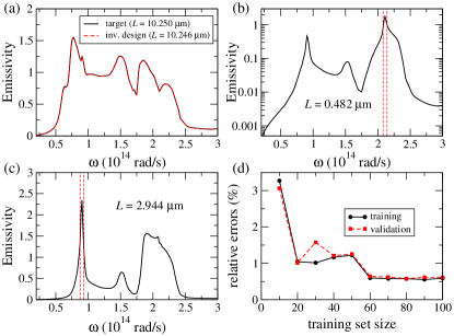
Figure 11: (a) Comparison of the NN approximation for the emissivity of a SiO₂ cube to a target spectrum for $L=10.250$ $\mu$m following the inverse design problem described in the text. (b,c) Result of the optimization problem where the emissivity of a SiO₂ cube in the frequency range defined by the vertical dashed lines is maximized while the emissivity outside is minimized. The obtained value of the optimal cube side is indicated in the panels. (d) Learning curves showing the mean relative error (training and validation) as a function of the training set size for the optimal NN simulating the emissivity of a SiO₂ cube.

Next, we illustrate the fact that the NN can also be used to solve optimization problems. In particular, we aim at determining what is the optimal cube side to maximize the emissivity at a given narrow frequency range while minimizing the emissivity outside this range. For this purpose, we fix the parameters of the NN, define a cost function for this task, and optimize the network with respect to the input parameters (the cube side in this problem). A convenient cost function in this case is defined as the ratio of the average of the emissivity inside the range of interest and the corresponding average outside that region: $E=\bar{\varepsilon}_{\mathrm{in}}/\bar{\varepsilon}_{\mathrm{out}}$. The results for this optimization problem for two ranges around the frequencies of the silica phonon polaritons are shown in Fig. 11(b,c), where we also indicate the corresponding optimal values of the cube side $L$. Notice that for the high-frequency phonon polariton (panel b), the emission is maximized for a relatively small cube, in which the emission comes from the whole body. For the low-frequency resonance (panel c) such an emission is maximized for a cube of size comparable to the skin depth, in which thermal emission is mainly a surface phenomenon.

The use of neural networks becomes particularly useful when there is lack of real (or training) data. In this sense, one may wonder how large the training set has to be in this case for the NN to be able to generalize well, i.e., to accurately predict spectra that have not been used in the training procedure. To answer this question, we analyzed the performance of our optimal NN as a function of the training set size. The corresponding learning curves are shown in Fig. 11(d) where one can see both the training and validation error expressed as the mean percent off per point on the spectrum. As seen, even training the NN with as little as 20 spectra, the validation error is on the order of $1$%, which illustrates how efficient NNs are at learning complex patterns like our emissivity spectra. Notice also that the evolution of the training and validation errors, which are very similar, shows that there is little overfitting, irrespective of the training set size.

Finally, having shown that simple NNs can efficiently learn the emissivity spectra of small objects, we also explored how to extend their use in this context. Thus, for instance, we tried and succeeded in using the NN trained on silica cubes to study the thermal emission of other simple objects such as spheres. Following the idea of transfer learning, we used the weights and biases of our NN as an initial starting point to train a network with the same architecture to learn the emissivity spectra of silica spheres of arbitrary radius (not shown here). As expected, this type of transfer learning substantially improves the accuracy of the training process and provides a promising path to model more demanding structures. In this sense, we are currently investigating if such an approach may be allow us to model structures like the silica nanoribbons mentioned above [86], which still remain out of the scope of any current theoretical method.

VI Conclusions

In summary, in this work we have reported the, to our knowledge, first systematic study of the application of deep learning techniques to the theoretical analysis of different radiative heat transfer phenomena. In particular, we have applied deep artificial neural networks to three state-of-the-art problems, ranging from near-field radiative heat transfer between multilayer systems to the description of the far-field thermal emission of extended systems in the context of passive radiative cooling and finite systems of arbitrary shape that defy Planck’s law. Despite the significant differences of the three studied scenarios, in all of them we have shown that, after training them on datasets of moderate size, simple neural network architectures can be used to do fast simulations of a great variety of thermal processes with a high precision. Moreover, we have demonstrated that neural networks can also be used as computational engines to solve interesting inverse design and optimization problems in the context of radiative heat transfer.

In this work, we have focused on proof-of-principle examples with the goal to illustrate some of the main ideas. We believe the concepts put forward here can be generalized to deal with much more complex structures and phenomena. Thus, for instance, it would of great interest to use the ideas discussed here in the context of heat transfer in many-body systems, a vast topic that is currently attracting a lot of attention [32]. Although we have mainly focused on the use of neural networks as function approximators, this is by no means the only possibility. It would also be very interesting to apply generative models to thermal radiation problems based on techniques like variational autoencoders (VAEs) or generative adversarial networks (GANs) [2]. Those techniques could, for instance, help to generate new data in situations where it is very hard to provide extensive training sets. This, in turn, could help to better train neural networks via data augmentation. On the other hand, less conventional networks like recurrent neural networks (RNNs) might find applications in the modeling of time-dependent thermal phenomena or in the development of protocols for thermal management. Overall, we believe that the application of deep learning to radiative heat transfer is still in its infancy and we hope this work can stimulate further research work aimed at exploring how artificial neural networks, and more generally artificial intelligence techniques, can contribute to accelerate the advance of this field.

- [1] Y. LeCun, Y. Bengio, and G. Hinton, Deep learning, Nature (London) 521, 436 (2015).
- [2] I. Goodfellow, Y. Bengio, and A. Courville, Deep Learning (MIT Press, Cambridge, MA, 2013).
- [3] C. C. Aggarwal, Neural Networks and Deep Learning (Springer, Cham, 2018).
- [4] A. Krizhevsky, I. Sutskever, G. E. Hinton, ImageNet classification with deep convolutional neural networks, In Proc. 25th Int. Conf. Neural Information Processing Systems 1097–1105 (NIPS, 2012).
- [5] K Cho, B. van Merrienboer, C. Gulcehre, D. Bahdanau, F. Bougares, H. Schwenk, Y. Bengio, Learning phrase representations using RNN encoder–decoder for statistical machine translation, in Proc. 2014 Conf. Empirical Methods in Natural Language Processing (EMNLP) 1724 (2014).
- [6] S. Shalev-Shwartz, S. Shammah, A. Shashua, Safe, multi-agent, reinforcement learning for autonomous driving, arXiv:1610.03295 (2016).
- [7] G. Hinton, L. Deng, D. Yu, G. E. Dahl, A. Mohamed, N. Jaitly, A. Senior, V. Vanhoucke, P. Nguyen, T. N. Sainath, and B. Kingsbury, Deep neural networks for acoustic modeling in speech recognition: the shared views of four research groups, IEEE Signal Proc. Mag. 29, 82 (2012).
- [8] P. Mehta, M. Bukov, C.-H. Wanga, A. G. R. Day, C. Richardson, C. K. Fisher, D. J. Schwab, A high-bias, low-variance introduction to Machine Learning for physicists, Phys. Rep. 810, 1 (2019).
- [9] G. Carleo, I. Cirac, K. Cranmer, L. Daudet, M. Schuld, N. Tishby, L. Vogt-Maranto, and L. Zdeborová, Machine learning and the physical sciences, Rev. Mod. Phys. 91, 045002 (2019).
- [10] F. Marquardt, Machine Learning and Quantum Devices, SciPost Phys. Lect. Notes 29 (2021).
- [11] Q.-J. Zhang, , Gupta, K. C. Gupta, and V. K. Devabhaktuni, Artificial neural networks for RF and microwave design-from theory to practice, IEEE Trans. Microw. Theory Tech. 51, 1339 (2003).
- [12] S. So, T. Badloe, J. Noh, J. Bravo-Abad, and J. Rho, Deep learning enabled inverse design in nanophotonics, Nanophotonics 9, 1041 (2020).
- [13] R. S. Hegde, Deep learning: a new tool for photonic nanostructure design, Nanoscale Adv. 2, 1007 (2020).
- [14] J. Jiang, M. Chen, and J. A. Fan, Deep neural networks for the evaluation and design of photonic devices, Nat. Rev. Mater. 6, 679 (2020).
- [15] W. Ma, Z. Liu, Z. A. Kudyshev, A. Boltasseva, W. Cai, and Y. Liu, Deep learning for the design of photonic structures, Nat. Photon. 16, 77 (2021).
- [16] D. Piccinotti, K. F. MacDonald, S. A. Gregory, I. Youngs, and N. I. Zheludev, Artificial intelligence for photonics and photonic materials, Rep. Prog. Phys. 84, 012401 (2021).
- [17] Z. Liu, D. Zhu, L. Raju, and W. Cai, Tackling Photonic Inverse Design with Machine Learning Adv. Sci. 8, 2002923 (2021).
- [18] J. Peurifoy, Y. Shen, L. Jing, Y. Yang, F. Cano-Renteria, B. G. DeLacy, J. D. Joannopoulos, M. Tegmark, M. Soljačić, Nanophotonic particle simulation and inverse design using artificial neural networks, Sci. Adv. 4, eaar4206 (2018).
- [19] Y. Qu, L. Jing, Y. Shen, M. Qiu, and M. Soljačić, Migrating Knowledge between Physical Scenarios Based on Artificial Neural Networks, ACS Photonics 6, 1168 (2019).
- [20] W. Ma, F. Cheng, and Y. Liu, Deep-Learning-Enabled On-Demand Design of Chiral Metamaterials, ACS Nano 12, 6326 (2018).
- [21] J. Jiang and J. A. Fan, Global Optimization of Dielectric Metasurfaces Using a Physics-Driven Neural Network, Nano Lett. 19, 5366 (2019).
- [22] D. Liu, Y. Tan, E. Khoram, and Z. Yu, Training Deep Neural Networks for the Inverse Design of Nanophotonic Structures, ACS Photonics 5, 1365 (2018).
- [23] S. An, C. Fowler, B. Zheng, M. Y. Shalaginov, H. Tang, H. Li, L. Zhou, J. Ding, A. M. Agarwal, C. Rivero-Baleine, K. A. Richardson, T. Gu, J. Hu, and H. Zhang, A Deep Learning Approach for Objective-Driven All-Dielectric Metasurface Design, ACS Photonics 6, 3196 (2019).
- [24] J. Jiang and J. A. Fan, Simulator-based Training of Generative Neural Networks for the Inverse Design of Metasurfaces, Nanophotonics 9, 1059 (2019).
- [25] R. Unni, K. Yao, and Y. Zheng, Deep Convolutional Mixture Density Network for Inverse Design of Layered Photonic Structures, ACS Photonics 7, 2703 (2020).
- [26] M. F. Modest, Radiative Heat Transfer (Academic Press, New York, 2013).
- [27] J. R. Howell, M. P. Mengüç,̧ R. Siegel, Thermal Radiation Heat Transfer, 6th ed.; (CRC Press: Boca Raton, FL, 2016).
- [28] Z. M. Zhang, Nano/Microscale Heat Transfer (McGraw-Hill: New York, 2007).
- [29] J. C. Cuevas and F. J. García-Vidal, Radiative Heat Transfer, ACS Photonics 5, 3896 (2018).
- [30] S. Basu, Z. M. Zhang, and C. J. Fu, Review of near‐field thermal radiation and its application to energy conversion, Int. J. Energy Res. 33, 1203 (2009).
- [31] B. Song, A. Fiorino, E. Meyhofer, and P. Reddy, Near-field radiative thermal transport: From theory to experiment, AIP Advances 5, 053503 (2015).
- [32] S.-A. Biehs, R. Messina, P. S. Venkataram, A. W. Rodriguez, J. C. Cuevas, P. Ben-Abdallah, Near-field radiative heat transfer in many-body systems, Rev. Mod. Phys. 93, 025009 (2021).
- [33] W. Li and S. Fan, Nanophotonic control of thermal radiation for energy applications, Opt. Express 26, 15995 (2018).
- [34] S. Fan, Thermal Photonics and Energy Applications, Joule 1, 264 (2017).
- [35] J. C. Cuevas, Thermal radiation from subwavelength objects and the violation of Planck’s law, Nat. Commun. 10, 3342 (2019).
- [36] Z. A. Kudyshev, A. V. Kildishev, V. M. Shalaev, Machine-learning-assisted metasurface design for high-efficiency thermal emitter optimization, Appl. Phys. Rev. 7, 021407 (2020).
- [37] D. P. Kingma and J. Ba, Adam: A Method for Stochastic Optimization, arXiv:1412.6980 (2014).
- [38] R. M. Schmidt, F. Schneider, and P. Hennig, Descending through a crowded valley — benchmarking deep learning optimizers, arXiv:2007.01547 (2021).
- [39] D. E. Rumelhart and D. Zipser, Feature discovery by competitive learning, Cogn. Sci. 9, 75 (1985).
- [40] D. E. Rumelhart, G. E. Hinton, and R. J. Williams, Learning representations by back-propagating errors, Nature 323, 533 (1986).
- [41] https://www.tensorflow.org
- [42] https://keras.io
- [43] D. Polder and M. Van Hove, Theory of radiative heat transfer between closely spaced bodies Phys. Rev. B 4, 3303 (1971).
- [44] Y. Guo, C. L. Cortes, S. Molesky, and Z. Jacob, Broadband super-Planckian thermal emission from hyperbolic metamaterials, Appl. Phys. Lett. 101, 131106 (2012).
- [45] S. A. Biehs, M. Tschikin, and P. Ben-Abdallah, Hyperbolic Metamaterials as an Analog of a Blackbody in the Near Field, Phys. Rev. Lett. 109, 104301 (2012).
- [46] Y. Guo and Z. Jacob, Thermal hyperbolic metamaterials, Opt. Express 21, 15014 (2013).
- [47] S.-A. Biehs, M. Tschikin, R. Messina, and P. Ben-Abdallah, Super-Planckian near-field thermal emission with phonon-polaritonic hyperbolic metamaterials, Appl. Phys. Lett. 102, 131106 (2013).
- [48] T. J. Bright, X. L. Liu, and Z. M. Zhang, Energy streamlines in near-field radiative heat transfer between hyperbolic metamaterials, Opt. Express 22, A1112 (2014).
- [49] O. D. Miller, S. G. Johnson, and A. W. Rodriguez, Effectiveness of Thin Films in Lieu of Hyperbolic Metamaterials in the Near Field, Phys. Rev. Lett. 112, 157402 (2014).
- [50] S.-A. Biehs and P. Ben-Abdallah, Near-field heat transfer between multilayer hyperbolic metamaterials, Z. Naturforsch. A 72, 115 (2017).
- [51] H. Iizuka and S. Fan, Significant enhancement of near-field electromagnetic heat transfer in a multilayer structure through multiple surface-states coupling, Phys. Rev. Lett. 120, 063901 (2018).
- [52] J. Song, Q. Cheng , L. Lu, B. Li, K. Zhou, B. Zhang, Z. Luo, and X. Zhou, Magnetically tunable near-field radiative heat transfer in hyperbolic metamaterials, Phys. Rev. Appl. 13 024054 (2020).
- [53] E. Moncada-Villa and J. C. Cuevas, Near-field radiative heat transfer between one-dimensional magnetophotonic crystals, Phys. Rev. B 103, 075432 (2021).
- [54] S. M. Rytov, Theory of Electric Fluctuations and Thermal Radiation, (Air Force Cambrige Research Center, Bedford, MA, 1953).
- [55] S. M. Rytov, Y. A. Kravtsov, and V. I. Tatarskii, Principles of Statistical Radiophysics, Vol. 3 (Springer-Verlag, Berlin Heidelberg, 1989).
- [56] B. Caballero, A. García-Martín, and J. C. Cuevas, Generalized scattering-matrix approach for magneto-optics in periodically patterned multilayer systems, Phys. Rev. B 85, 245103 (2012).
- [57] E. Moncada-Villa, V. Fernández-Hurtado, F. J. García-Vidal, A. García-Martín, and J. C. Cuevas, Magnetic field control of near-field radiative heat transfer and the realization of highly tunable hyperbolic thermal emitters, Phys. Rev B 92, 125418 (2015).
- [58] V. Fernández-Hurtado, F.J. García-Vidal, Shanhui Fan, J.C. Cuevas, Enhancing Near-Field Radiative Heat Transfer with Si-based Metasurfaces, Phys. Rev. Lett. 118, 203901 (2017).
- [59] E. Rephaeli, A. Raman, and S. Fan, Ultrabroadband Photonic Structures to Achieve High-Performance Daytime Radiative Cooling, Nano Lett. 13, 1457 (2013).
- [60] A. P. Raman, M. A. Anoma, L. Zhu, E. Rephaeli, and S. Fan, Passive radiative cooling below ambient air temperature under direct sunlight, Nature (London) 515, 540 (2014).
- [61] M. M. Hossain, B. Jia, M. Gu, A metamaterial emitter for highly efficient radiative cooling. Adv. Opt. Mater. 3, 1047 (2015).
- [62] A. R. Gentle and G. B. Smith, A subambient open roof surface under the mid-summer Sun, Adv. Sci. 2, 1500119 (2015).
- [63] Z. Chen, L. Zhu, A. Raman, S. Fan, Radiative cooling to deep sub-freezing temperatures through a 24-h day-night cycle, Nat. Commun. 7, 13729 (2016).
- [64] J. Kou, Z. Jurado, Z. Chen, S. Fan, A. J. Minnich, Daytime radiative cooling using near-black infrared emitters, ACS Photonics 4, 626 (2017).
- [65] Y. Zhai, Y. Ma, S. N. David, D. Zhao, R. Lou, G. Tan, R. Yang, X. Yin, Scalable-manufactured randomized glass-polymer hybrid metamaterial for daytime radiative cooling, Science 355, 1062 (2017).
- [66] E. A. Goldstein, A. P. Raman, and S. Fan, Sub-ambient non-evaporative fluid cooling with the sky, Nat. Energy 2, 17143 (2017).
- [67] J. Mandal, Y. Fu, A. C. Overvig, M. Jia, K. Sun, N. N. Shi, H. Zhou, X. Xiao, N. Yu, Y. Yang, Hierarchically porous polymer coatings for highly efficient passive daytime radiative cooling, Science 362, 315 (2018).
- [68] T. Li, Y. Zhai, S. He, W. Gan, Z. Wei, M. Heidarinejad, D. Dalgo, R. Mi, X. Zhao, J. Song, J. Dai, C. Chen, A. Aili, A. Vellore, A. Martini, R. Yang, J. Srebric, X. Yin L. Hu, A radiative cooling structural material, Science 364, 760 (2019).
- [69] L. Zhou, H. Song, J. Liang, M. Singer, M. Zhou, E. Stegenburgs, N. Zhang, C. Xu, T. Ng, Z. Yu, B. Ooi, and Q. Gan, A polydimethylsiloxane-coated metal structure for all-day radiative cooling, Nat. Sustain. 2, 718 (2019).
- [70] D. Zhao, A. Aili, Y. Zhai, S. Xu, G. Tan, X. Yin, and R. Yang, Radiative sky cooling: fundamental principles, materials, and applications, Appl. Phys. Rev. 6, 021306 (2019).
- [71] W. Li and S. Fan, Radiative cooling: harvesting the coldness of the universe, Opt. Photon. News 30, 32 (2019).
- [72] D. Li, X. Liu, W. Li, Z. Lin, B. Zhu, Z. Li, J. Li, B. Li, S. Fan, J. Xie and J. Zhu, Scalable and hierarchically designed polymer film as a selective thermal emitter for high-performance all-day radiative cooling, Nat. Nanotechnol. 16, 153 (2021).
- [73] IR Transmission Spectra, Gemini Observatory Kernel Description. http://www.gemini.edu/?q/node/10789, accessed Aug 10, 2018.
- [74] L. Zhu, A. P. Raman, and S. Fan, Radiative cooling of solar absorbers using a visibly transparent photonic crystal thermal blackbody, Proc. Natl. Acad. Sci. U.S.A. 112, 12282 (2015).
- [75] E. D. Palik, Handbook of Optical Constants of Solids (Academic Press, London, 1985).
- [76] H. U. Yang, J. D’Archangel, M. L. Sundheimer, E. Tucker, G. D. Boreman, and M. B. Raschke, Optical dielectric function of silver, Phys. Rev. B 91, 235137 (2015).
- [77] J. Gu, Z. Wang, J. Kuen, L. Ma, A. Shahroudy, B. Shuai, T. Liu, X. Wang, G. Wang, J. Cai, and Tsuhan Chen, Recent advances in convolutional neural networks, Pattern Recognition, 77, 354 (2018).
- [78] M. Planck, The Theory of Thermal Radiation (P. Blakiston Son & Co., Philadelphia, 1914).
- [79] C. F. Bohren and D. R. Huffman, Absorption and Scattering of Light by Small Particles (Wiley, New York, 1998).
- [80] J. A. Schuller, T. Taubner, and M. L. Brongersma, Optical Antenna Thermal Emitters, Nat. Photon. 3, 658 (2009).
- [81] G. W. Kattawar and M. Eisner, Radiation from a Homogeneous Isothermal Sphere, Appl. Opt. 9, 2685 (1970).
- [82] V. A. Golyk, M. Krüger, and M. Kardar, Heat radiation from long cylindrical objects, Phys. Rev. E 85, 046603 (2012).
- [83] V. Fernández-Hurtado, A. I. Fernández-Domínguez, J. Feist, F. J. García-Vidal, and J. C. Cuevas, Super-Planckian far-field radiative heat transfer, Phys. Rev. B 97, 045408 (2018).
- [84] D.Thompson, L. Zhu, R. Mittapally, S. Sadat, Z. Xing, P. McArdle, M. M. Qazilbash, P. Reddy, and E. Meyhofer, Hundred-fold enhancement in far-field radiative heat transfer over the blackbody limit, Nature (London) 561, 216 (2018).
- [85] C. Wuttke and A. Rauschenbeutel, Thermalization Via Heat Radiation of an Individual Object Thinner than the Thermal Wavelength, Phys. Rev. Lett. 111, 024301 (2013).
- [86] S. Shin, M. Elzouka, R. Prasher, and R. Chen, Far-field coherent thermal emission from polaritonic resonance in individual anisotropic nanoribbons, Nat. Commun. 10, 1377 (2019).
- [87] C. R. Otey, L. Zhu, S. Sandhu, and S. Fan, Fluctuational electrodynamics calculations of near-field heat transfer in non-planar geometries: A brief overview, J. Quant. Spectrosc. Radiat. Transfer 132, 3 (2014).
- [88] A. W. Rodriguez, M. T. H. Reid, and S. G. Johnson, Fluctuating-surface-current formulation of radiative heat transfer: Theory and applications, Phys. Rev. B 88, 054305 (2013).
- [89] M. T. H. Reid and S. G. Johnson, Efficient computation of power, force and torque in BEM scattering calculations, IEEE T. Antenn. Propag. 63, 3588 (2015).
- [90] A. G. Polimeridis, M. T. H. Reid, W. Jin, S. G. Johnson, J. K. White, and A. W. Rodriguez, Fluctuating volume-current formulation of electromagnetic fluctuations in inhomogeneous media: Incandescence and luminescence in arbitrary geometries, Phys. Rev. B 92, 134202 (2015).
- [91] R. M. Abraham Ekeroth, A. García-Martín, and J. C. Cuevas, Thermal discrete dipole approximation for the description of thermal emission and radiative heat transfer of magneto-optical systems, Phys. Rev. B 95, 235428 (2017).
- [92] E. M. Purcell and C. R. Pennypacker, Scattering and Absorption of Light by Nonspherical Dielectric Grains, Astrophys. J. 186, 705 (1973).
- [93] M. A. Yurkin and A. G. Hoekstra, The discrete dipole approximation: An overview and recent developments, J. Quant. Spectrosc. Radiat. Transfer 106, 558 (2007).
- [94] M. Krüger, T. Emig, and M. Kardar, Nonequilibrium Electromagnetic Fluctuations: Heat Transfer and Interactions, Phys. Rev. Lett. 106, 210404 (2011).
- [95] M. Krüger, G. Bimonte, T. Emig, and M. Kardar, Trace formulas for nonequilibrium Casimir interactions, heat radiation, and heat transfer for arbitrary objects, Phys. Rev. B 86, 115423 (2012).
- [96] G. James, D. Witten, T. Hastie, R. Tibshirani, An Introduction to Statistical Learning (Springer, New York, 2017).