Estimating the case fatality rate of a disease during the course of an epidemic with an application to COVID-19 in Argentina

Abstract

We present an accurate estimator of the case fatality rate that can be computed during the course of an epidemic outbreak and we prove its asymptotic properties. We apply it to the real case of covid-19 in Argentina during 2020 and to simulated data and show its very good performance.

(1) Instituto de Ciencias, Universidad de General Sarmiento

(2) Departamento de matemática, Facultad de Ciencias Exactas y Naturales, Universidad de Buenos Aires

(3) Instituto de Cálculo, Universidad de Buenos Aires - CONICET

1 Introduction

One of the most important questions when a new infectious disease arises, as Covid-19, is to know how deadly it is, that is to say, to know the proportion of infected people that dies. Note that the term infected includes confirmed and some unconfirmed cases, that are nevertheless infected. This proportion is known as infection fatality rate (ifr). This rate is a key epidemiological measure for quantifying disease severity and is particularly important during outbreaks of emerging infectious diseases such as Covid-19. It is difficult to estimate this rate during the course of an outbreak for several reasons: the great number of cases which are never diagnosed, bias from reporting delays and the time gap between diagnosis and death (see Baud et al. (2020)). Since the Covid- 19 information is limited to confirmed cases and, in general, the real number of infected people remains unknown due to the presence of asymptomatic cases or patients with very mild symptoms, we focus on the proportion of diagnosed people that dies. Traditionally, the “naive”case fatality rate over a certain period of time (a day, a week, a month, the whole epidemic) is understood as the proportion of people diagnosed over this period of time who die from the disease in the same period. The World Health Organization and many countries report this naive case fatality rate on a daily basis, considering the period of time from the beginning of the epidemic up to that day. The reason for using this rate is that it requires minimum information for computation and eventually equals the final case fatality rate when the epidemic is over, see Kim et al. (2021). This rate has a tendency to underestimation, so many other estimators have been proposed to reduce the bias. There have been many attempts to define and calculate the case fatality rate for Covid-19, see for instance, Chang et al. (2020) and Shim et al. (2020). Lipsitch et al. (2015) and Marschner (2021) define the case fatality rate as the probability of death from the disease among confirmed cases and discuss the potential biases in its estimation. Another attempt in this direction is made in Lee and Lim (2019). Most of the rates mentioned so far, use data of daily recovered patients. The data base publicly available in Argentina does not include this information. Garske et al. (2009) proposed a definition of case fatality rate that can be computed with minimum information.

The rate informed in Argentina daily during the Covid-19 pandemic underestimates the true case fatality rate since the estimation is made on day t by dividing the number of deceased people from Covid-19 until day t by the number of confirmed cases until day t. The denominator also includes confirmed cases that have not yet died from the disease, but will do so in the future. Thus, the delay between confirmation and death might result in bias when estimating the case fatality rate in this naive way. This bias may be high, especially when the estimation is made in a moment of rapid growth of confirmed cases or if the time between diagnosis and death is long. At the beginning of the outbreak, the number of cofirmed cases may double in a few days. However, only a small proportion of the patients that will finally die, do so in the first days after diagnosis.

In this work we define the case fatality rate until day t ($cfr(t)$) as the expected proportion of confirmed cases that die or will die from Covid-19 infection among cases confirmed since the beginning of the epidemic until day t included. The defined $cfr(t)$ could be called cumulative case fatality rate but, for simplicity, we will refer to it as case fatality rate by day $t$. We propose an unbiased estimator of $cfr(t)$. This estimation is achieved by accounting for the expected future fatalities. Garske et al. (2009) attempt to correct the problem of the time gap between diagnosis and death. The estimator of $cfr(t)$ they propose is unbiased if the probability of death among confirmed cases each day is constant in time but it may be biased if these probabilities change. In this work, we propose an estimator of $cfr(t)$ that can be computed on day $t$ and we show that it is unbiased even when the probability of death among confirmed cases is not constant in time. We apply our proposal, Garske et al’s estimator and the naive estimator and compare them in the real case of Covid-19 in Argentina during 2020 as well as in simulated data and we show the very good performance of our proposal.

The paper is organized as follows. In Section 2 we introduce the main definitions and notations, including the definition of $cfr(t)$ together with the proposed estimators and confidence intervals for $cfr(t)$. In Section 3 we report the results of a simulation study. In Section 4 we apply the proposed estimators to the real data set from Argentina in 2020. In section 5 we comment on how we estimate the distribution of time between diagnosis and death for patients who died. In Section 6 we summarize the concluding remarks. Finally, in the Appendix we present the proofs of the assymptotic properties of the proposed estimator.

2 Main definitions and notation

We shall denote random variables with upper case letters and non random parameters with lower case letters. We define

• $p_{d}$ the probability of death among cases confirmed during day $d$.

• $c_{d}$ the number of cases confirmed during day $d$.

• $M_{d,i}$ a dichotomous variable that equals $1$ if the $i$–th confirmed case on day $d$ dies because of the disease and $0$ if it does not.

• $M_{d,i}(t)$ a dichotomous variable that equals $1$ if the $i$–th confirmed case on day $d$ has died because of the disease by day $t$ and $0$ if it has not, defined for $d\leq t$.

• $M_{f}(t)$ the total number of persons that die from Covid-19 infection among cases confirmed until day $t$ included, once the epidemic has ended.

• $M(t)$ the number of confirmed cases that died from Covid-19 from the beginning of the epidemic (day $0$), until day $t$ inclusive.

Suppose that $M_{d,1},\ldots,M_{d,c_{d}}$ are i.i.d. with a Bernoulli distribution with probability of success $p_{d}$, i.e. $M_{d,i}\sim\mbox{Be}(p_{d})$. Observe that

$$M_{f}(t)=\sum\limits_{d=0}^{t}\sum\limits_{i=1}^{c_{d}}M_{d,i}\,\,\text{ while }\,\,M(t)=\sum_{d=0}^{t}\sum_{i=1}^{c_{d}}M_{d,i}(t).$$ (1)

We call $CFR_{N}$ the naive estimator of the case fatality rate that is usually reported on day $t$. With this notation, this estimator is

$$CFR_{N}(t)=\frac{M(t)}{\sum_{d=0}^{t}c_{d}}.$$ (2)

We define $CFR_{F}(t)$ as the proportion of cases confirmed unitl day $t$ which finally die because of the disease, and refer to this proportion as the final case fatality rate by day $t$. In terms of the defined variables we have that

$$CFR_{F}(t)=\frac{M_{f}(t)}{\sum_{d=0}^{t}c_{d}}\,.$$ (3)

Notice that $CFR_{F}(t)$ cannot be computed on day $t$; one would have to wait for all the diagnosed people by day $t$ to recover or die. We define the case fatality rate by day $t$ as the expected value of $CFR_{F}(t)$, i.e, $cfr(t)=\mathbb{E}\left(CFR_{F}(t)\right)$. It is worth noting that the case fatality rate by $t$ defined in this way is a population parameter and it is not observable, not even at the end of the epidemic. Using (1), we easily obtain

$$cfr(t)=\sum\limits_{d=0}^{t}c_{d}p_{d}/\sum\limits_{d=0}^{t}c_{d}=\sum\limits_{d=0}^{t}\omega_{d}p_{d}.$$ (4)

$cfr(t)$ is a weihted sum of daily case fatality rates $p_{d}$, where each day’s weight is the proportion of cases that was confirmed that day with respect to the total number of cases confirmed until day $t$. $cfr(t)$ can be interpreted as the probability of dying from the disease for a randomly picked person among those diagnosed by day $t$. If $p_{d}=p$ ($p_{d}$ is constant all along the epidemic), $cfr(t)=p$. We remark that $cfr(t)$ is the parameter of interest, of which the case fatality rate observed at the end of the epidemic is an observation. In order to estimate $cfr(t)$ we define

$T_{d,i}=$ Number of days since confirmation until death in the $i$-th case confirmed on day $d$.

Let $F_{d}$ be the cumulative distribution function ($cdf$) of $T_{d,i}|M_{d,i}=1$. Several authors use this distribution in their estimations, see for instance Marschner (2021), Garske et al. (2009), Nishiura et al. (2009), Dorigatti et al. (2020). Note that we are allowing the $cdf$ to change in time unlike Garske et al. (2009). This seems realistic for several reasons; for instance, new treatments may lengthen the survival time, the sanitary system may collapse and this may shorten the survival time or the confirmation of cases may be faster, lengthening also the time from confirmation until death, among others.

2.1 Proposed estimators

2.1.1 An unbiased estimator of $cfr(t)$

Our goal is to predict on day $t$ the number of people that eventually will die, among confirmed cases until day $t$, that is to say $M_{f}(t)$, as defined in (1). The idea of our proposal is the following: we know that, among the cases confirmed on day $d$, with $d\leq t$, the expected proportion that will have died by day $t$, among those that have died or will die eventually is $F_{d}(t-d)$. Therefore, dividing the cases confirmed during day $d$ that have died by day $t$ by $F_{d}(t-d)$, we will obtain a predictor of the number of confirmed cases during day $d$ that will finally die. In concrete, we define the predictor of $M_{f}(t)$ as follows:

$$\widehat{M}_{f}(t)=\sum\limits_{d=0}^{t}\displaystyle\frac{\sum\limits_{i=1}^{c_{d}}M_{d,i}(t)}{F_{d}(t-d)}$$

We then estimate the case fatality rate by day $t$, $cfr(t)$, by

$$CFR(t)=\widehat{M}_{f}(t)/\sum\limits_{d=0}^{t}c_{d}.$$ (5)

Note that the probability of dying from covid by day $t$ for a case confirmed on day $d$ can be expressed in the following way

$$\mathbb{P}(M_{d,i}(t)=1) = \mathbb{P}(M_{d,i}=1)\cdot\mathbb{P}(T_{d,i}\leq t-d|M_{d,i}=1)$$

$$= p_{d}F_{d}(t-d).$$

Straightforward calculations show that $\mathbb{E}(CFR(t))=cfr(t)$ and, therefore, the proposed estimator is unbiased. Setting $Z_{d,i}(t)=M_{d,i}(t)/F_{d}(t-d)$, we see that $CFR(t)$ is an average of the $Z_{d,i}(t)$ variables, which are independent but not necessarily identically distributed since $M_{d,i}(t)\sim Be(p_{d}F_{d}(t-d))$. However, since the sequence of variables satisfy the Lindemberg condition (under certain conditions, see appendix) we will be able to build an asymptotic $(1-\alpha)\cdot 100\%$ confidence interval for the expected value of the average, which is $cfr(t)$. The confidence interval takes the form $CFR(t)\pm z_{1-\alpha/2}\sqrt{V(CFR(t))}$, where

$$V(CFR(t))=\frac{\sum_{d=0}^{t}c_{d}p_{d}(1-p_{d}F_{d}(t-d))/F_{d}(t-d)}{r_{t}^{2}}$$ (6)

and $r_{t}=\sum_{d=0}^{t}c_{d}$ is the total number of variables. The estimator $CFR(t)$ can only be used if $F_{d}$ is known. Since this is not the case when we work with real data, we will replace it by an estimator $\hat{F}_{d}$, see Section 5. Therefore, the predictor we will actually use for real data is

$$\widehat{M}_{f}(t)=\sum\limits_{d=0}^{t}\left(\sum\limits_{i=1}^{c_{d}}M_{d,i}(t)\right)/{\hat{F}_{d}(t-d)}.$$

To build the confidence interval on day $t$ we also need the $p_{d}$ values for $0\leq d\leq t$, which we do not have in a real data analysis. In such case, for $t_{0}\leq t_{1}$, call $cfr_{t_{0}}^{t_{1}}$ the expected proportion of people that dies from Covid-19 between those who are confirmed in the period of time from $t_{0}$ to $t_{1}$ days after the start of the epidemic. In order to estimate $p_{d^{*}}$ on day $t$, for $d^{*}\leq t$ we propose to use an estimator of $cfr_{d^{*}-3}^{d^{*}+3}$ based on the same idea of the cumulative case fatality rate estimator $CFR$, as follows:

$$\hat{p}_{d^{*}}=CFR_{d^{*}-3}^{d^{*}+3}(t)=\displaystyle\frac{\sum\limits_{d=d^{*}-3}^{d^{*}+3}(\sum\limits_{i=1}^{c_{d}}M_{d,i}(t))/F_{d}(t-d)}{\sum\limits_{d=d^{*}-3}^{d^{*}+3}c_{d}}\,.$$ (7)

We compute estimation (7) for days $d^{*}$, with $3\leq d^{*}\leq t-3$ and we estimate $\hat{p}_{d^{*}}=\hat{p}_{t-3}$ for $t-2\leq d^{*}\leq t$ and $\hat{p}_{d^{*}}=\hat{p}_{3}$ for $0\leq d^{*}\leq 2$. Estimation of $p_{d}$ is here used as an auxiliary calculus in order to estimate the variance of the confidence intervals but it is a problem of interest in its own since it allows to estimate the actual probability of dying from Covid-19 for the cases confirmed on day $d$. An analogous calculation can be done in order to estimate the daily probability of needing an intensive care unit (ICU), which might be useful in order to predict the number of people who will arrive to ICU. This may be the subject of future work.

2.1.2 Modified Garske et al. (2009) estimator

Garske et al. (2009) do not consider the possibility that the distribution of the time from confirmation to death, $F_{d}$ or the daily case fatality rate $p_{d}$ may vary with time. Their estimator of the case fatality rate is defined as follows

$$CFR_{G}(t)=\frac{M(t)}{\sum\limits_{d=0}^{t}c_{d}F(t-d)}.$$ (8)

Where $F$ is the distribution of the time from confirmation to death and $M(t)$ is the random variable that counts the number of confirmed cases that died from the beginning of the epidemic (day $0$), to day $t$. If we consider varying $F_{d}$ their estimator becomes

$$CFR_{G}^{M}(t)=\frac{M(t)}{\sum\limits_{d=0}^{t}c_{d}F_{d}(t-d)}.$$

Simple computations yield

$$\mathbb{E}(CFR_{G}^{M}(t))=\frac{\sum\limits_{d=0}^{t}c_{d}F_{d}(t-d)p_{d}}{\sum\limits_{d=0}^{t}c_{d}F_{d}(t-d)}=\sum\limits_{d=0}^{t}\omega^{*}_{d}p_{d}.$$ (9)

Equation (9) shows that the expected value of this estimator is a weighted mean of $p_{d}$, but the weights are not the same as in $cfr(t)$ and therefore, the estimator is not necessarily unbiased, unless $p_{d}=p$ for all $d$. Of course these estimators are also computed by replacing $F$ or $F_{d}$ by their estimates.

Despite this bias, Garske et al’s estimator has some advantages if $p_{d}$ is constant. First, if the distribution function $F_{d}=F$ is known or estimated previously, it can be computed for day $t$ using only the number of confirmed cases and the number of deaths until day $t$. The estimator we propose, on the other hand, requires knowing the number of deaths by day $t$, among all confirmed cases on day $d$, for all $d\leq t$.

3 Monte Carlo study

To evaluate the performance of the proposed estimators, we performed a Monte Carlo study. The hypothetical epidemic develops in the following way. For the first 158 days it has the same number of daily cases $c_{d}$ as we had in Argentina from March 3rd until august 7th, 2020. During the subsequent 158 days, the daily cases diminish in such a way that the curve is symmetric. That is to say, $c_{158+d}=c_{157-d}$ for $0\leq d\leq 157$. Then, from $d\geq 316$ onwards, we set $c_{d}\equiv 0$. For each confirmed case on day $d$ we set its probability of dying from covid in $p_{d}$. For $p_{d}$ we consider the following setting: $p_{d}=c_{1}I_{[0,d^{*}-1]}(d)+c_{2}I_{[d^{*},315]}(d)$, where $d^{*}$ is the day in which $p_{d}$ changes and $315$ is the day of the last confirmed case. We consider $d^{*}\in\{90,120\}$ and we vary $c_{1}$ and $c_{2}$ in $\{0.02,0.05,0.1\}$ with $c_{1}\neq c_{2}$. For those who die from the disease, we set a survival time since confirmation of $F_{d}\equiv F$, using $F=\mbox{BN}(\mu=10.79,r=0.88)$. This distribution has been seen to provide a good fit in the real case of Argentina by August 2020, and the values of the parameters are the maximum likelihood estimates. In all cases we calulate all the estimators presented in Section 2.1, namely $CFR_{N}(t)$, $CFR(t)$ and $CFR_{G}(t)$, as defined in equations (2), (5) and (8), respectively. In order to calculate $CFR(t)$ and $CFR_{G}(t)$ we do it in two different ways. At a first instance we make the estimation using the known distribution of survival times $F$ used to generate the data, and in such case we make the estimation for all times $t$, for $0\leq t\leq t_{f}$, where $t_{f}$ is the final day of epidemic, i.e., every confirmed case has either died or recovered from Covid by $t_{f}$. At the second instance we estimate the distribution $F$ by what we call the “empirical estimation” $\hat{F}_{emp}$ in the way described in section 5. Since for the empirical estimation of $F_{d}$, we analyze the survival time of cases confirmed 45 days before day $t$ (see Section 5), at this second instance we calculate the estimators for days $t$ with $90\leq t\leq t_{f}$. At both instances we calculate $95\%$ confidence intervals for $cfr(t)$ presented in Section 2.1: $CFR(t)\pm z_{0.975}\sqrt{V(CFR(t))}$. Since $V(CFR(t))$ depends both on the daily case fatality rates $p_{d}$ and on the distribution functions $F_{d}$ for $0\leq d\leq t$, for the first instance estimation we use the known $p_{d}$ values and the known $F_{d}\equiv F$ distribution used to generate the data while for the second instance estimation we used the empirical estimation $\hat{F}_{emp}$ as the estimate of the $F_{d}$ and we performed the estimation of the daily $p_{d}$ presented in (7). For the derivation of the confidence intervals, see the Appendix.

We compare three estimators of the case fatality rate by day $t$ that can be computed on day $t$, namely $CFR_{N}(t)$, $CFR(t)$ and $CFR_{G}(t)$ with $cfr(t)$. The three estimators are defined in equations (2), (5) and (8), respectively

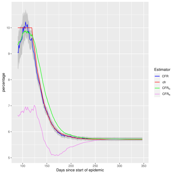
In Figure 1 we observe the $cfr(t)$ values and its estimators together with the confidence intervals based on $CFR$, presented as a shaded band around $CFR(t)$. The graph corresponds to the scenario of an estimated $F$ with parameters $c_{1}=0.1$, $c_{2}=0.05$ and $d^{*}=120$, i.e., the daily case fatality rates jump from $0.1$ to $0.05$ on day $120$ since the beginning of the epidemic. One can observe that the $CFR$ estimator works very well in the whole epidemic as well as the confidence intervals which contain $cfr(t)$ during almost the whole epidemic. The estimator proposed by Garske et al. (2009), $CFR_{G}$, overestimates $cfr(t)$ for a long period of time after day $120$, the day when the cumulative case fatality rates $cfr(t)$ start to decrease. On the other hand one observes that the “naive” case fatality rate $CFR_{N}$ underestimates $cfr(t)$ during most of the epidemic. At the end of the epidemic all the estimators work well.

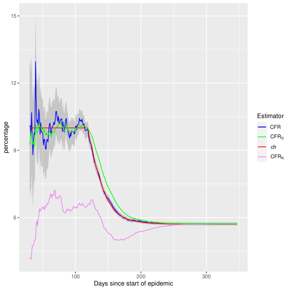
In Figure 2 we observe the same scenario as in Figure 1 but using the known $F$ for the estimators and also the known $p_{d}$ values to calculate the variance of the confidence intervals. We graph since day $30$ from the start of epidemic because there are few cases and much noise during the first month. In addition to Figure 1 comments we can observe here the unbiased behaviour of $CFR_{G}$ while $p_{d}$ and $cfr(t)$ values remain constant, until day $120$. In that period a lower variability of $CFR_{G}$ estimator compared to $CFR$ is observed as well. Again after day $120$ when the $cfr(t)$ values start to change a better behaviour of $CFR$ estimator, as compared to $CFR_{G}$, is observed. The same comments of Figures 1 and 2 apply to all scenarios we have studied and so we only present these two graphs.

Figure 1: Case fatality rate estimated by different methods in simulated data, generated using $p_{d}=0.1$ until day 120 and $p_{d}=0.05$ after day 120.

Figure 2: Case fatality rate estimated by different methods in simulated data, generated using $p_{d}=0.1$ until day 120 and $p_{d}=0.05$ after day 120, assuming $F$ is known.

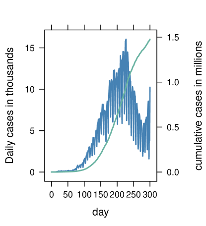
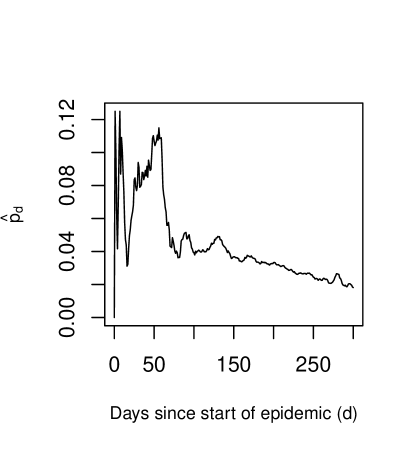
In the Appendix we prove that the proposed confidence intervals (C.I.) have assympthotic level $(1-\alpha)\times 100\%$. However, it is desirable to have an idea of how many confirmed cases we need in order for the C.I. to have approximately the desired level. To deal with this interest we performed a simulation study. To generate the data we made $1000$ replicates. In each replication, we used $c_{d}$, the number of confirmed cases of the first $301$ days of the epidemic in Argentina, see Figure 3. For each day $d$, the value of $p_{d}$ used is the proportion of confirmed cases which finally died between those cases confirmed between days $d-3$ and $d+3$, i.e, during the week centered at $d$, see Figure 4. We used $F_{d}\equiv F$ where $F$ is a Zero Inflated Negative Binomial (ZINB) distribution, i.e., a convex combination of $F_{0}$, the distribution of a constantly zero variable, and $F_{1}$ a negative binomial distribution. We set $F=\pi F_{0}+(1-\pi)F_{1}$, where $\pi=0.103$, and $F_{1}\sim NB(\mu=12.59,r=1.2191)$, where the values of the parameters correspond to the maximium likelihood ZINB estimate for the distribution $F$ of the survival times since diagnosis for people who died from Covid and were confirmed positive during the first $300$ days of the epidemic in Argentina. For each replication we built the confidence interval $(a(t),b(t))$ estimating $F_{d}$ with $\hat{F}_{emp}$ as in the former simulation and also estimating the $p_{d}$ values, as it was explained in (7). For each replication we checked for every $t$ with $90\leq t\leq 301$ whether the real interval contained the case fatality rate by day $t$, $cfr(t)$ or not. Then, for each $t$ we measured the proportion of times between the $1000$ replications in which $a(t)\leq cfr(t)\leq b(t)$, and we call that proportion the “mean coverage” of the intervals at time $t$.

Figure 3: Blue line is for daily cases and green line for cumulative cases.

Figure 4: Proportion of confirmed cases which finally died among those cases confirmed between days $d-3$ and $d+3$ in the first $300$ days of the epidemic in Argentina

Figure 5: Blue line is for mean coverage and green line for mean length of intervals.

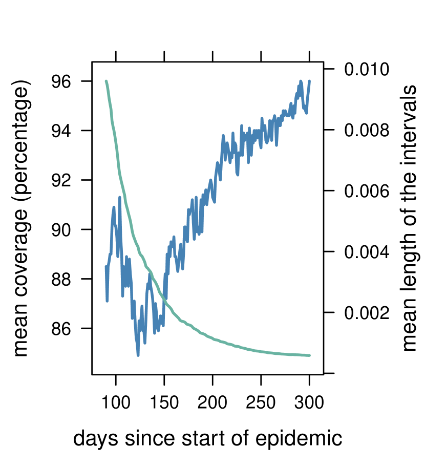
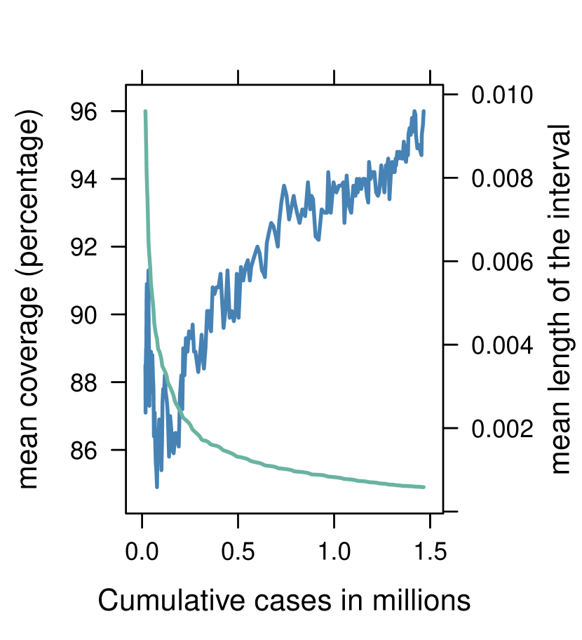
In Figure 5 (left) we observe that since day $90$ of the epidemic the C.I. have “mean coverage” greater than $85\%$, since day $200$ approximately the “mean coverage” is greater than $90\%$ and the mean coverage approaches $95\%$ when $t$ approaches $300$. In Figure 5 (right) we see how the “mean coverage” behaves depending on the number of cases, and see that for more than $500,000$ cases the “mean coverage” is over $90\%$ and that the coverage is around $95\%$ when the number of cases is around $1,500,000$.

4 Real data: the Covid-19 epidemic in Argentina

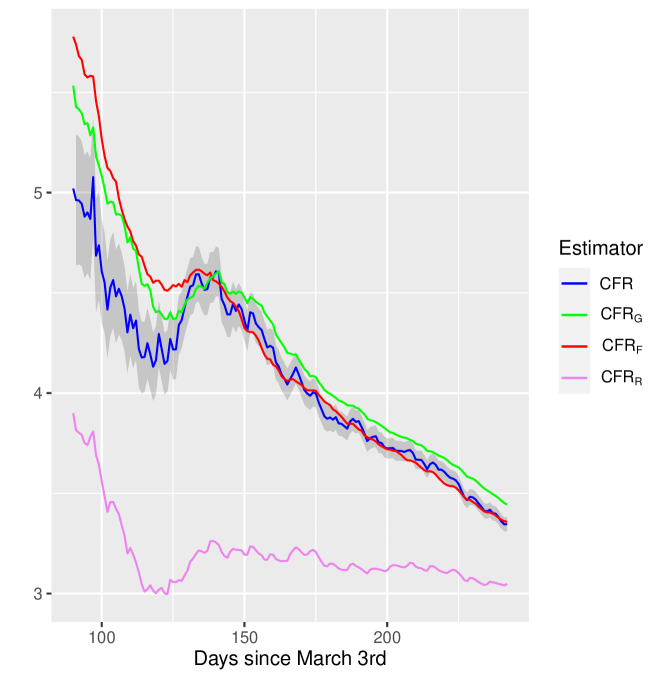
In this section we analise the behaviour of the estimators presented in Section 2.1 in a real data example. Of course, in this case, we cannot compare the values of the estimators with the value of interest $cfr(t)$ because this value is not observable. The natural way to deal with this problem is to compare the estimators to the final case fatality rate by day $t$, $CFR_{F}(t)$. We compute, for each day $t$ from June 1st to December 31st 2020, different estimators of $cfr(t)$ using the data base from the Ministry of Health of Argentina as of April 4th, 2021. We compare three estimators of the case fatality rate by day $t$, $cfr(t)$, that can be computed on day $t$, namely $CFR_{N}(t)$, $CFR(t)$ and $CFR_{G}(t)$ to the final case fatality rate until day $t$ observed on April 4th, which we call $CFR_{F}(t)$, assuming that all the confirmed cases during 2020 have either recovered or die by that date. The three estimators are defined in equations (2), (5) and (8), respectively, and $CFR_{F}(t)$ is computed by

$$CFR_{F}(t)=\frac{\sum_{d=0}^{t}\sum_{i=1}^{c_{d}}M_{d,i}(t_{F})}{\sum_{d=0}^{t}c_{d}}$$ (10)

where $t_{F}$ is the number of days from March 3rd 2020 to April 4th 2021. Observe that $CFR_{F}(t)$ defined in (10) equals the one defined in (3) if all people diagnosed until day $t$ have already died or recovered by day $t_{F}$, which might not be true but both values should be very close one from the other. In fact, the Argentine data set shows that the $0.98$ quantile of the times between confirmation and death is $45$ days and that the proportion of dead among cases confirmed during 2020 that died in 90 days or less is $0.9967$.

Figure 6 displays the estimated curves, together with the observed $CFR_{F}(t)$. First, observe that both $CFR_{G}(t)$ and $CFR(t)$ do a much better job than the usual $CFR_{N}(t)$ at estimating $cfr(t)$, since they are both much closer to $CFR_{F}(t)$. Second, we remark that $CFR_{G}(t)$ is nearer to $CFR_{F}(t)$ until around day $110$ but soon after that day, the biased nature of $CFR_{G}(t)$ becomes apparent. Our simulations (unreported here) show that $CFR_{G}(t)$ has less variability than $CFR(t)$. However, since for both estimators the variance converges to zero as the number of observations goes to infinity, the weight of the variance in the bias-variance trade off gets smaller and smaller as the number of cases rises. By day 150 approximately, we begin to see clearly that $CFR_{G}(t)$ is biased and converges to a different value, not the $cfr(t)$ we are trying to estimate. Finally we would like to remark that the most realistic thing to do would have been to use the data base reported on day $t$ to compute the estimators, for each $t$ in the analysis, instead of using the data base of April 4th for all the estimations. This was not possible because we did not have all the data bases from june to december of 2020. However, we had access to some data bases from june 2020 and we observed (in estimations not reported here) that the estimators did not work as well as those we report here. The reason is the problem of delays in entering data, i.e., many people who was already a confirmed case and a dead case by day $t$, only appear in the data base of day $t$ as a confirmed case, but not as a dead case, whereas if we take a posterior data base (say, a two month later data base), these people appear correctly as diagnosed and dead by day $t$. This problem of delays in entering the data may be dealt with nowcasting techniques, see for example Bastos et al. (2019). This may be subject of further work.

Figure 6: Case fatality rate of Covid-19 in Argentina in 2020 estimated by different methods

5 Estimation of $F_{d}$

We now explain briefly how we estimate $F_{d}$, for $d\leq t$. For such estimation, we assume that $F_{d}\equiv F$ for all $d$ and, on day $t$, we estimate $F_{d}(k)$ by $\hat{F}_{emp}(k)$, the proportion of confirmed cases who died in $k$ or less days since confirmation, among those who died form the disease. For estimating this proportion we consider only cases who were confirmed by day $t-45$ and dead by day $t$. The reason for considering only cases confirmed 45 days before the day of interest is that in the Argentine data set, approximately $98\%$ of confirmed cases that die, do so in 45 days or less. Considering all confirmed cases until day $t$ would lead to an overestimation of $F(k)$, for small values of $k$. We studied different estimators of $F$, assuming parametric models for this distribution, including regression of $y$ on $x$ with $y=$ number of days from diagnosis to death and $x$= number of days from the beginning of the epidemic (March 3rd in this case) until diagnosis date. We fitted a linear model and different generalized linear models. However for the vast majority of values of $t$ the regressions were non significant. Moreover, it was necessary to use the fitted models to estimate $F_{d}$ for values of $d$ that were way out of the range of the training data. This induced large extrapolation errors. We believe this problem can be solved by estimating with techniques designed for censored data. This does not seem simple for this kind of data and may be the subject of further work.

6 Concluding remarks

Given the diagnosed cases of an epidemic disease we set a statistical model for the outcomes of the disease for patients diagnosed in different days. Based on the model, we define the case fatality rate of the disease by day $t$ as the probability of dying from the disease for a randomly picked person among those diagnosed by day $t$ and we propose an estimator for this rate. This estimator is based on the distribution of the times between confirmation and death of confirmed cases that die because of the disease.

We prove that the proposed estimator is unbiased, consistent and asymptotically normal and we derive asymptotic confidence intervals. Both the estimator and confidence intervals for the case fatality rate can be computed during the course of the epidemic.

We show the very good performance of the proposed estimator and the confidence intervals for large samples, as compared to the estimator proposed by Garske et al. (2009), by means of a Monte Carlo study and an analysis of the Covid-19 epidemic in Argentina during 2020.

We also performe a Monte Carlo simulation to study the mean coverage of the asymptotic confidence intervals as a function of the cumulative number of cases and we show that it is very near the nominal confidence level when the number of cases is large.

We also propose an estimator of the daily case fatality rate and an extension of the estimator proposed by Garske et al. (2009) that allows the distribution of the times between confirmation and death to change in time.

Appendix

In this section we prove the consistency and asymptotic normality of the $CFR(t)$. We call consistency of $CFR(t)$ to the fact that $CFR(t)-cfr(t)\buildrel p\over{\longrightarrow}0$, as $t\to\infty$. First of all, recall the Central Limit Theorem for triangular arrays.

Theorem 1

Suppose that for each $t\in\mathbb{N}_{0}$, $X_{t,1},X_{t,2},\ldots,X_{t,r_{t}}$ are independent random variables. Let $S_{t}=X_{t,1}+X_{t,2}+\ldots+X_{t,r_{t}}$. Suppose that $\mathbb{E}(X_{t,k})=0$ for all $t$ and $k$, and that the variances $\mathbb{E}(X_{t,k}^{2})$ are finite. Call $\sigma_{t}^{2}=\mbox{\sc Var}(S_{t})$. If the Lindemberg condition is satisfied, i.e.:

$$\lim_{t\to\infty}\frac{1}{\sigma_{t}^{2}}\sum_{k=1}^{r_{t}}\mathbb{E}\left[X_{t,k}^{2}\cdot\mathbf{1}_{\{|X_{t,k}|>\varepsilon s_{t}\}}\right]=0$$

for all $\varepsilon>0$, where $\mathbf{1}_{\{\cdots\}}$ is the indicator function, then the central limit theorem holds, i.e. $S_{t}/\sigma_{t}\buildrel D\over{\longrightarrow}{\mathcal{N}}(0,1)$

Proof. See Theorem 27.2 in Billingsley (2008)

For a collection of variables $M_{d,i}(t)$, with $t\geq 0$, $0\leq d\leq t$ and $1\leq i\leq c_{d}$, and distributions $F_{d}$ for $d\geq 0$ defined as in Section 2, define the following assumptions:

A1 $\inf_{d}F_{d}(0)=D>0$.
A2 $\inf_{d}p_{d}=I>0$.
A3 $\sup_{d}p_{d}=S<1$.

Theorem 2

For each $t\in\mathbb{N}$, let $\{M_{d,i}(t)\}_{d,i}$ for $0\leq d\leq t$ and $1\leq i\leq c_{d}$ be independent random variables ${Be(p_{d}F_{d}(t-d))}$. Assume that the total number of confirmed cases until day $t$, $r_{t}=\sum_{d=0}^{t}c_{d}\stackrel{{\scriptstyle t\to\infty}}{{\longrightarrow}}\infty$. Then

$(i)$ If A1 holds, then $CFR(t)-cfr(t)\buildrel p\over{\longrightarrow}0\,,$

$(ii)$ If A1 to A3 hold, then $\frac{CFR(t)-cfr(t)}{\sqrt{V(CFR(t))}}\stackrel{{\scriptstyle D}}{{\longrightarrow}}N(0,1).$

Proof. Even though weak consistency is a consequence of asymptotic normality, we write the proof of part $(i)$ because it is interesting in itself and has a simple proof independent of $(ii)$.

The estimator $CFR(t)$ we propose for the case fatality rate, $cfr(t)$, is a sample average of the variables $Z_{d,i}(t)=M_{d,i}(t)/F_{d}(t-d)$. Easy calculations show that $\mathbb{E}(Z_{d,i}(t))=p_{d}$ and $V(Z_{d,i}(t))=p_{d}(1-p_{d}F_{d}(t-d))/F_{d}(t-d)$ are finite.

$(i)$ Since A1 holds, we get

$$V(Z_{d,i}(t))\leq\frac{1}{\inf_{d^{\prime}}{F_{d^{\prime}}(0)}}-\inf_{d^{\prime}}p_{d^{\prime}}\leq\frac{1}{D},$$

for all $d$ and for all $i$. Then

$$V(CFR(t))=\frac{\sum_{d=0}^{t}c_{p}V(Z_{d,i}(t))}{r_{t}^{2}}\leq\frac{1}{Dr_{t}}\stackrel{{\scriptstyle t\to\infty}}{{\longrightarrow}}0,$$

since $r_{t}\stackrel{{\scriptstyle t\to\infty}}{{\longrightarrow}}\infty$. Since $CFR(t)$ is an unbiased estimator of $cfr(t)$, this implies that $CFR(t)-cfr(t)\buildrel p\over{\longrightarrow}0$.

$(ii)$ For each day $t$ by taking the centered variables $Z_{d,i}(t)-p_{d}$ for $0\leq d\leq t$ and $1\leq i\leq c_{d}$, we have $r_{t}$ independent variables of mean $0$. If we rename these variables as $X_{t,1},\ldots,X_{t,r_{t}}$, we will see that the Lindemberg condition of Theorem 1 is satisfied and then if $S_{t}=X_{t,1}+X_{t,2}+\ldots+X_{t,r_{t}}$ and $\sigma_{t}^{2}=\mbox{\sc Var}(S_{t})$, the convergence in distribution $S_{t}/\sigma_{t}\buildrel D\over{\longrightarrow}{\mathcal{N}}(0,1)$ is obtained. The proof concludes by observing with elementary calculations that

$$\frac{CFR(t)-cfr(t)}{\sqrt{\mbox{\sc Var}(CFR(t))}}=\frac{S_{t}}{\sigma_{t}}\,.$$

Let us see that the variables $\{Z_{d,i}(t)-p_{d}\}_{d,i}$ satisfy the Lindemberg condition. We have that

$$V(Z_{d,i}(t))\geq(\inf_{d^{\prime}}p_{d^{\prime}})(1-\sup_{d^{\prime}}p_{d^{\prime}})=I(1-S),$$

for all $d$ and for all $i$. This implies

$$\sigma_{t}^{2}=\sum_{d=0}^{t}\sum_{i=1}^{c_{d}}V(Z_{d,i}(t))\geq r_{t}I(1-S)$$

and then $\sigma_{t}\to\infty$ as $r_{t}\to\infty$. We observe that the variable $Z_{d,i}(t)-p_{d}$ takes only two possible values: $-p_{d}$ and $1/F_{d}(t-d)-p_{d}$, so we get that

$$|Z_{d,i}(t)-p_{d})|\leq\max\left\{1,\frac{1}{\inf_{d}{F_{d}(0)}}-\inf_{d^{\prime}}p_{d^{\prime}}\right\}\leq\max\left\{1,\frac{1}{D}\right\}=M.$$

Given $\varepsilon>0$, if $r_{t}$ is large enough, then $\varepsilon\cdot\sigma_{t}>M$ and ${\mathbf{1}_{\{|Z_{d,i}(t)-p_{d}|>\varepsilon\sigma_{t}\}}=0}$ for all $d$ and $i$, and then the Lindemberg condition

$$\lim_{t\to\infty}\frac{1}{\sigma_{t}^{2}}\sum_{d=0}^{t}\sum_{i=1}^{c_{d}}\mathbb{E}\left[(Z_{d,i}(t)-p_{d})^{2}\cdot\mathbf{1}_{\{|Z_{d,i}(t)-p_{d}|>\varepsilon\sigma_{t}\}}\right]=0$$

is satisfied.

References

- Bastos et al. (2019) Bastos, L.S., Economou, T., Gomes, M.F., Villela, D.A., Coelho, F.C., Cruz, O.G., Stoner, O., Bailey, T., Codeço, C.T., 2019. A modelling approach for correcting reporting delays in disease surveillance data. Statistics in medicine 38, 4363–4377.
- Baud et al. (2020) Baud, D., Qi, X., Nielsen-Saines, K., Musso, D., Pomar, L., Favre, G., 2020. Real estimates of mortality following covid-19 infection. The Lancet infectious diseases 20, 773.
- Billingsley (2008) Billingsley, P., 2008. Probability and measure. John Wiley & Sons.
- Chang et al. (2020) Chang, C.S., Yeh, Y.T., Chien, T.W., Lin, J.C.J., Cheng, B.W., Kuo, S.C., 2020. The computation of case fatality rate for novel coronavirus (covid-19) based on bayes theorem: An observational study. Medicine 99.
- Dorigatti et al. (2020) Dorigatti, I., Okell, L., Cori, A., Imai, N., Baguelin, M., Bhatia, S., Boonyasiri, A., Cucunubá, Z., Cuomo-Dannenburg, G., FitzJohn, R., et al., 2020. Report 4: severity of 2019-novel coronavirus (ncov). Imperial College London, London .
- Garske et al. (2009) Garske, T., Legrand, J., Donnelly, C.A., Ward, H., Cauchemez, S., Fraser, C., Ferguson, N.M., Ghani, A.C., 2009. Assessing the severity of the novel influenza a/h1n1 pandemic. Bmj 339.
- Kim et al. (2021) Kim, B., Kim, S., Jang, W., Jung, S., Lim, J., 2021. Estimation of the case fatality rate based on stratification for the covid-19 outbreak. PloS one 16, e0246921.
- Lee and Lim (2019) Lee, S., Lim, J., 2019. Online estimation of the case fatality rate using a run-off triangle data approach: An application to the korean mers outbreak in 2015. Statistics in medicine 38, 2664–2679.
- Lipsitch et al. (2015) Lipsitch, M., Donnelly, C.A., Fraser, C., Blake, I.M., Cori, A., Dorigatti, I., Ferguson, N.M., Garske, T., Mills, H.L., Riley, S., et al., 2015. Potential biases in estimating absolute and relative case-fatality risks during outbreaks. PLoS neglected tropical diseases 9, e0003846.
- Marschner (2021) Marschner, I.C., 2021. Case fatality risk estimated from routinely collected disease surveillance data: application to covid–19. Biostatistics & Epidemiology , 1–20.
- Nishiura et al. (2009) Nishiura, H., Klinkenberg, D., Roberts, M., Heesterbeek, J.A., 2009. Early epidemiological assessment of the virulence of emerging infectious diseases: a case study of an influenza pandemic. PloS one 4, e6852.
- Shim et al. (2020) Shim, E., Mizumoto, K., Choi, W., Chowell, G., 2020. Estimating the risk of covid-19 death during the course of the outbreak in korea, february–may 2020. Journal of clinical medicine 9, 1641.