Testing the Early Universe with Anisotropies of the Gravitational Wave Background

Ema Dimastrogiovanni    Matteo Fasiello    Ameek Malhotra    P. Daniel Meerburg    and Giorgio Orlando
Abstract

In this work we analyse in detail the possibility of using small and intermediate-scale gravitational wave anisotropies to constrain the inflationary particle content. First, we develop a phenomenological approach focusing on anisotropies generated by primordial tensor-tensor-scalar and purely gravitational non-Gaussianities. We highlight the quantities that play a key role in determining the detectability of the signal. To amplify the power of anisotropies as a probe of early universe physics, we consider cross-correlations with CMB temperature anisotropies. We assess the size of the signal from inflationary interactions against so-called induced anisotropies. In order to arrive at realistic estimates, we obtain the projected constraints on the non-linear primordial parameter FNLsubscript𝐹NLF_{\rm NL} for several upcoming gravitational wave probes in the presence of the astrophysical gravitational wave background. We further illustrate our findings by considering a concrete inflationary realisation and use it to underscore a few subtleties in the phenomenological analysis.

1 Introduction

The advent of laser interferometers has opened up a new era for gravitational wave (GW) astronomy. From the very first direct detection [1] of a GW event in 2015 we have learned precious lessons in stellar evolution and astrophysics. The growing number of GW events detected also provides the ideal testing ground for general relativity. In this sense, the GW170817 event and its optical counterpart have been especially consequential [2, 3, 4]. Operational and upcoming GW detectors hold the potential to bring about transformative changes also in cosmology and the particle physics of the early universe. The increasing number and sensitivity of laser interferometers (LIGO/Virgo/Kagra, LISA, Taiji, Einstein Telescope(ET), Cosmic Explorer (CE) to mention but a few), together with the possibility of detecting GWs at intermediate scales via pulsar timing arrays (PTA) puts us in the enviable position to access key information on cosmological GW sources and, possibly, distinguish their signal from the astrophysical GW background.

Mechanism for GW production are abound in the early universe [5]. Gravitational waves are a universal prediction of inflation and may also result from pre-heating dynamics, the energy loss of cosmic strings via gravitational radiation, and first order phase transitions (this typically requires beyond-the-Standard-Model physics). In this work we will focus on the stochastic gravitational wave background (SGWB) from inflation. We shall be interested in probing inflationary (self)interactions, and thus the particle content of the very early universe, through GW probes at intermediate and small scales (from the 109superscript10910^{-9} Hz of PTAs to the 10kHz of, for example, LIGO).
A GW signal at PTA scales or at the frequency range accessible via laser interferometers is typically associated to a multi-field or multi-clock inflationary realisation111The proposed Big Bang Observer (BBO) is an exception in that it might be able to detect even a signal from single-field slow roll models provided that the tensor-to-scalar ratio r𝑟r is close to the current combined Planck + BICEP2/Keck Array BK15 upper bound of r<0.056𝑟0.056r<0.056 [6]. There are interesting proposals for single-field models generating a GW signal detectable at small scales. One such mechanism [7] postulates the existence of a non-attractor phase followed by an attractor solution [8].. Detection of a primordial SGWB of inflationary origin would then by itself be strongly suggestive of a rich inflationary field content. In this manuscript we take the analysis one step further and detail on how one may use GW probes to test inflation beyond the “standard” power spectrum (i.e. beyond the quadratic Lagrangian). Anisotropies of the GW spectrum are the key observables here, and in particular those engendered by primordial tensor-tensor-scalar (TTS) and purely GW (TTT) non-Gaussianities.
Primordial non-Gaussianities are well constrained on large scales by cosmic microwave background (CMB) observations [9, 10]. The physics of the intermediate and small scales constraints is also very interesting. As show in [11, 12], propagation effects suppress e.g. the primordial TTT signal in most of the momentum configurations. Let us offer an intuitive understanding of such suppression. Direct access to the bispectrum at intermediate/small scales requires that the modes have all entered the horizon during radiation domination and thus have accumulated a history of propagation through structure. Given that the momenta are to be different in view of the overall momentum conservation, different modes have different propagation history, so much so that this “washes out” any initial correlation, i.e. any correlation due to the initial conditions set by inflation.
A proven way to get around this suppression is to consider specific momenta configurations, such as the ultra-squeezed one [13]. In this configuration there is one long (up to horizon-size) mode and two short ones222Another momenta configuration that can be probed is the folded one, see for example [14].. This implies that only small modes can be accessed directly, but it also guarantees a much milder suppression: a very long mode does not suffer suppression effects and the two short ones may have a much more similar propagation history, thereby avoiding the wash out effect. The anisotropies we shall study in this work probe precisely this momentum configuration and therefore provide a precious handle on non-Gaussianities at intermediate and small scales333For alternative examples of probes of primordial non-Gaussianities, see e.g. [15, 16, 17, 18, 19, 20, 21, 22, 23, 24, 25, 26]..
We will explore the constraining power of anisotropies on primordial physics in two steps. First, we will consider anisotropies due to non-trivial squeezed primordial TTS and TTT bispectra. Second, we will study the cross-correlation of such GW anisotropies with temperature anisotropies of the CMB. As we shall see, the latter observable can take us a long way towards verifying the primordial nature of possible GW anisotropies even in the presence of a large stochastic GW background of astrophysical origin.
We find it worthwhile in this manuscript to first provide a phenomenological, agnostic, approach to anisotropies from primordial long-short mode couplings, without committing to any specific inflationary model. It will allow us to show what is typically expected in terms of observables and single out the key quantities that determine the likelihood for a given signal to be observed. Besides the usual suspects, i.e. the non-linear parameters FNLttssubscriptsuperscript𝐹ttsNLF^{\rm tts}_{\rm NL}, FNLtttsubscriptsuperscript𝐹tttNLF^{\rm ttt}_{\rm NL} and the tensor-to-scalar ratio r𝑟r, we will see how e.g. cross-correlations are also rather sensitive to the angular dependence of primordial bispectra.
Our analysis would be incomplete without a detailed example of an inflationary mechanism that supports a GW signal on small scales as well as a sufficiently large primordial non-Gaussian amplitude to give the leading contribution to GW anisotropies, beyond the ever-present induced component [27, 28, 29, 30]. To this aim, we employ an EFT formulation of the inflationary Lagrangian comprising an extra444That is, beyond the massless spin-2 field of general relativity. spin-2 field non-minimally coupled to the inflaton [31, 32]. Such coupling is necessary to weaken unitarity bounds on the spin-2 particle mass range (see e.g. [33, 34]), thus allowing it to have a small (compared to the Hubble rate H𝐻H) mass.
This paper is organised as follows. In Section 2 we briefly review induced anisotropies and compare them with those generated by primordial non-Gaussianities. We give a rule of thumb criterion to estimate the size of each contribution. We study the case of both monopolar and quadrupolar-type contributions to GW anisotropies from a TTS correlator, providing both the general result and its simplified analytical expression in the scale-invariant case. The contribution to anisotropies due to a primordial TTT correlation is also scrutinised.
Section 3 is devoted to cross-correlations with the CMB temperature anisotropies. After reviewing the induced contribution, we focus on cross-correlating the TTS term with the CMB and derive the projected constraints on FNLttssubscriptsuperscript𝐹ttsNLF^{\rm tts}_{\rm NL} from a range of GW probes: PTAs, LISA&Taiji, ET&CE, and BBO. We also account for the presence of an astrophysical gravitational wave background (AGWB), which allows us to highlight the power of cross-correlations: a primordial signal may be detected even if the AGWB dominates over the primordial SGWB. The TTT contribution to cross-correlations is also analysed.
In Section 4 we consider a specific inflationary realisation and show how, interestingly, in this specific case it is the TTT primordial correlation that provides the leading contribution both at the level of the auto- and the cross-correlation. This is true despite the factor of r𝑟r suppression any TTT correlator inherits with respect to its TTS counterpart. We find that an instrument such as BBO can deliver a percent level relative error on FNLtttsubscriptsuperscript𝐹tttNLF^{\rm ttt}_{\rm NL} in this model. We discuss our findings and comment on future work in Section 5.

2 SGWB anisotropies

Cosmological backgrounds of gravitational waves (CGWB) are typically characterised in terms of the their normalised energy density [35],

ΩGW(k)1ρcrdρGWdlnk,subscriptΩGW𝑘1subscript𝜌cr𝑑subscript𝜌GW𝑑𝑘\displaystyle{\Omega_{{\rm{{GW}}}}}(k)\equiv\frac{1}{\rho_{\rm{cr}}}\frac{d\rho_{\rm GW}}{d\ln k}\,, (2.1)

where ρGWsubscript𝜌GW\rho_{\rm GW} is the energy density of GW and ρcrsubscript𝜌cr\rho_{\rm cr} is the critical energy density. For the primordial GW background from inflation, the energy density observed today at time η0subscript𝜂0\eta_{0} is related to the primordial tensor power spectrum as

ΩGW(k,η0)=k212a02H02𝒯2(k,η0)14πd2n^𝒫γ(𝐤,𝐝,ηin),subscriptΩGW𝑘subscript𝜂0superscript𝑘212superscriptsubscript𝑎02superscriptsubscript𝐻02superscript𝒯2𝑘subscript𝜂014𝜋superscript𝑑2^𝑛subscript𝒫𝛾𝐤𝐝subscript𝜂in\displaystyle{\Omega_{{\rm{{GW}}}}}(k,\eta_{0})=\frac{k^{2}}{12a_{0}^{2}H_{0}^{2}}\mathcal{T}^{2}(k,\eta_{0})\cdot\frac{1}{4\pi}\int d^{2}\hat{n}\,\mathcal{P}_{\gamma}(\mathbf{k},\mathbf{d},\eta_{\rm in})\,, (2.2)

where 𝒯(k,η0)𝒯𝑘subscript𝜂0\mathcal{T}(k,\eta_{0}) is the tensor transfer function [36] and 𝐤=kn^𝐤𝑘^𝑛\mathbf{k}=k\hat{n}. The primordial power spectrum is evaluated at the point 𝐝=dn^𝐝𝑑^𝑛\mathbf{d}=-d\hat{n} with d=η0ηin𝑑subscript𝜂0subscript𝜂ind=\eta_{0}-\eta_{\rm in} being the conformal time elapsed from horizon-entry of the mode k𝑘k to the present. Allowing for anisotropies in the energy density we can write the above quanitity as

ΩGW(f)=Ω¯GW(f)[1+14πd2n^δGW(f,n^)],subscriptΩGW𝑓subscript¯ΩGW𝑓delimited-[]114𝜋superscript𝑑2^𝑛subscript𝛿GW𝑓^𝑛\displaystyle{\Omega_{{\rm{{GW}}}}}(f)=\overline{\Omega}_{\rm GW}(f)\Big{[}1+\frac{1}{4\pi}\int d^{2}\hat{n}\,\delta_{\rm GW}(f,\hat{n})\Big{]}\,, (2.3)

where δGWsubscript𝛿GW\delta_{\rm GW} and Ω¯GW(f)subscript¯ΩGW𝑓\overline{\Omega}_{\text{\tiny GW}}(f) denote the anisotropic and isotropic component of the energy density respectively. For a generic cosmological gravitational wave background, these anisotropies can arise from (i) propagation in the perturbed universe, and (ii) an inhomogeneous production mechanism. We shall refer to these anisotropies as ‘induced’ and ‘intrinsic’, respectively.

2.1 Induced anisotropies

The induced anisotropies arise from the propagation of GW through the large scale scalar perturbations of the universe555There is also a contribution from the large scale tensor peturbations but similar to the CMB, this is subdominant compared to the contribution from the scalar perturbations [28, 29].. Note that such anisotropies are universal in nature, in the sense that they are rather model-independent. These anisotropies have been studied using the standard Boltzmann formalism in [27, 28, 29, 37]. Similarly to what happens with the CMB, one finds that the SGWB is affected by both the Sachs-Wolfe (SW) and Integrated Sachs-Wolfe (ISW) effects. On large angular scales, the dominant contribution is given by the SW term which can be written as [28, 29]

δindGW[4lnΩGW(k)lnk]d3q(2π)3eidn^𝐪23ζ(q).similar-to-or-equalssubscriptsuperscript𝛿GWinddelimited-[]4subscriptΩGW𝑘𝑘superscript𝑑3𝑞superscript2𝜋3superscript𝑒𝑖𝑑^𝑛𝐪23𝜁𝑞\displaystyle\delta^{\rm{{GW}}}_{\rm ind}\simeq\left[4-\frac{\partial\ln{{\Omega_{{\rm{{GW}}}}}(k)}}{\partial\ln{k}}\right]\int\frac{d^{3}q}{(2\pi)^{3}}e^{-id\hat{n}\cdot\mathbf{q}}\cdot\frac{2}{3}\zeta(\vec{q})\,. (2.4)

2.2 Intrinsic anisotropies from primordial non-Gaussianity

The instrinsic anisotropies of interest here are those arising from large primordial non-Gaussianities in the squeezed limit, i.e. primordial bispectra of the form γ𝐤1γ𝐤2X𝐪0delimited-⟨⟩subscript𝛾subscript𝐤1subscript𝛾subscript𝐤2subscript𝑋𝐪0\langle\gamma_{\mathbf{k}_{1}}\gamma_{\mathbf{k}_{2}}\,X_{\mathbf{q}\to 0}\rangle. Here X𝐪subscript𝑋𝐪X_{\mathbf{q}} denotes a long wavelength mode of either a scalar or tensor perturbation while γ𝐤1,2subscript𝛾subscript𝐤12\gamma_{\mathbf{k}_{1,2}} are the short wavelength tensor modes which we take to be at interferometer scales (these modes re-enter the horizon during radiation domination). Let us begin with the case where the long mode X𝐪subscript𝑋𝐪X_{\mathbf{q}} corresponds to the long wavelength mode of the primordial curvature perturbation ζ𝜁\zeta. The existence of this coupling between the long modes ζ𝐪subscript𝜁𝐪\zeta_{\mathbf{q}} and the short modes γ𝐤subscript𝛾𝐤\gamma_{\mathbf{k}} modulates the primordial power spectrum as [17, 38, 39, 18, 40, 41],

𝒫γmod(𝐤,𝐱)=λ𝒫γλ(k)[1+qkd3q(2π)3ei𝐪𝐱FNLλ,tts(𝐤,𝐪)ζ(𝐪)],subscriptsuperscript𝒫mod𝛾𝐤𝐱subscript𝜆subscriptsuperscript𝒫𝜆𝛾𝑘delimited-[]1subscriptmuch-less-than𝑞𝑘superscript𝑑3𝑞superscript2𝜋3superscript𝑒𝑖𝐪𝐱superscriptsubscript𝐹NL𝜆tts𝐤𝐪𝜁𝐪\displaystyle\mathcal{P}^{\rm mod}_{\gamma}(\mathbf{k},\mathbf{x})=\sum_{\lambda}\mathcal{P}^{\lambda}_{\gamma}(k)\left[1+\int_{q\ll k}\frac{d^{3}q}{(2\pi)^{3}}\,e^{i\mathbf{q}\cdot\mathbf{x}}F_{\rm NL}^{\lambda,\rm tts}(\mathbf{k},\mathbf{q})\zeta(\mathbf{q})\right]\,, (2.5)

where

FNLλ,tts(𝐤,𝐪)=Bttsλ(𝐤𝐪/2,𝐤𝐪/2,𝐪)Pζ(q)Pγλ(k),superscriptsubscript𝐹NL𝜆tts𝐤𝐪subscriptsuperscript𝐵𝜆tts𝐤𝐪2𝐤𝐪2𝐪subscript𝑃𝜁𝑞subscriptsuperscript𝑃𝜆𝛾𝑘\displaystyle F_{\rm NL}^{\lambda,\rm tts}(\mathbf{k},\mathbf{q})=\frac{B^{\lambda}_{\rm tts}(\mathbf{k}-\mathbf{q}/2,-\mathbf{k}-\mathbf{q}/2,\mathbf{q})}{P_{\zeta}(q)P^{\lambda}_{\gamma}(k)}, (2.6)

and the primordial bispectrum Btts(𝐤1,𝐤2,𝐤3)subscript𝐵ttssubscript𝐤1subscript𝐤2subscript𝐤3B_{\rm tts}(\mathbf{k}_{1},\mathbf{k}_{2},\mathbf{k}_{3}) in the squeezed limit is defined as

γ𝐤1λγ𝐤2λζ𝐤30=δλλBTTSλ(𝐤1,𝐤2,𝐤3).superscriptdelimited-⟨⟩superscriptsubscript𝛾subscript𝐤1𝜆superscriptsubscript𝛾subscript𝐤2superscript𝜆subscript𝜁subscript𝐤30superscript𝛿𝜆superscript𝜆subscriptsuperscript𝐵𝜆TTSsubscript𝐤1subscript𝐤2subscript𝐤3\displaystyle\langle\gamma_{\mathbf{k}_{1}}^{\lambda}\gamma_{\mathbf{k}_{2}}^{\lambda^{\prime}}\zeta_{\mathbf{k}_{3}\to 0}\rangle^{\prime}=\delta^{\lambda\lambda^{\prime}}B^{\lambda}_{\rm TTS}(\mathbf{k}_{1},\mathbf{k}_{2},\mathbf{k}_{3})\,. (2.7)

The prime here denotes the fact that we have omitted the factor of (2π)3δ(3)(𝐤1+𝐤2+𝐤3)superscript2𝜋3superscript𝛿3subscript𝐤1subscript𝐤2subscript𝐤3(2\pi)^{3}\,\delta^{(3)}(\mathbf{k}_{1}+\mathbf{k}_{2}+\mathbf{k}_{3}) that ensures momentum conservation. Note that while in principle it is possible to have polarisation-dependent power spectra and bispectra and hence FNLλ1,ttsFNLλ2,ttssuperscriptsubscript𝐹NLsubscript𝜆1ttssuperscriptsubscript𝐹NLsubscript𝜆2ttsF_{\rm NL}^{\lambda_{1},\rm tts}\neq F_{\rm NL}^{\lambda_{2},\rm tts} for the different helicities λ1λ2subscript𝜆1subscript𝜆2\lambda_{1}\neq\lambda_{2}, this shall not be the case for the inflationary models we will consider here. Hence, in what follows further we will write FNLλ,ttsFNLttssuperscriptsubscript𝐹NL𝜆ttssubscriptsuperscript𝐹ttsNLF_{\rm NL}^{\lambda,\rm tts}\equiv F^{\text{tts}}_{\rm NL} and Eq. (2.5) becomes,

𝒫γmod(𝐤,𝐱)=𝒫γ(k)[1+qkd3q(2π)3ei𝐪𝐱FNLtts(𝐤,𝐪)ζ(𝐪)].subscriptsuperscript𝒫mod𝛾𝐤𝐱subscript𝒫𝛾𝑘delimited-[]1subscriptmuch-less-than𝑞𝑘superscript𝑑3𝑞superscript2𝜋3superscript𝑒𝑖𝐪𝐱subscriptsuperscript𝐹ttsNL𝐤𝐪𝜁𝐪\displaystyle\mathcal{P}^{\rm mod}_{\gamma}(\mathbf{k},\mathbf{x})=\mathcal{P}_{\gamma}(k)\left[1+\int_{q\ll k}\frac{d^{3}q}{(2\pi)^{3}}\,e^{i\mathbf{q}\cdot\mathbf{x}}F^{\text{tts}}_{\rm NL}(\mathbf{k},\mathbf{q})\zeta(\mathbf{q})\right]\,. (2.8)

The isotropic and anisotropic666In the context of the Boltzmann formalism for GW [27, 28, 29], these anisotropies are captured by the initial condition term. components of the energy density can then be expressed in terms of this primordial tensor power spectrum as

Ω¯GW(k,η0)=k212a02H02𝒯2(k,η0)𝒫γ(k)subscript¯ΩGW𝑘subscript𝜂0superscript𝑘212superscriptsubscript𝑎02superscriptsubscript𝐻02superscript𝒯2𝑘subscript𝜂0subscript𝒫𝛾𝑘\displaystyle\overline{\Omega}_{\text{\tiny GW}}(k,\eta_{0})=\frac{k^{2}}{12a_{0}^{2}H_{0}^{2}}\mathcal{T}^{2}(k,\eta_{0})\mathcal{P}_{\gamma}(k) (2.9)

and

δttsGW(k,n^)=qkd3q(2π)3eidn^𝐪FNLtts(𝐤,𝐪)ζ(q).subscriptsuperscript𝛿GWtts𝑘^𝑛subscriptmuch-less-than𝑞𝑘superscript𝑑3𝑞superscript2𝜋3superscript𝑒𝑖𝑑^𝑛𝐪subscriptsuperscript𝐹ttsNL𝐤𝐪𝜁𝑞\displaystyle\delta^{\rm{{GW}}}_{\rm tts}(k,\hat{n})=\int_{q\ll k}\frac{d^{3}q}{(2\pi)^{3}}\,e^{-id\hat{n}\cdot\mathbf{q}}F^{\text{tts}}_{\rm NL}(\mathbf{k},\mathbf{q})\zeta(\vec{q})\,. (2.10)

We also consider here the anisotropies generated from the modulation of the power spectrum by a long wavelength tensor mode [13],

𝒫γmod(𝐤,𝐱)=𝒫γ(k)[1+qkd3q(2π)3ei𝐪𝐱FNLttt(𝐤,𝐪)λγλ(𝐪)ϵijλ(q^)n^in^j],subscriptsuperscript𝒫mod𝛾𝐤𝐱subscript𝒫𝛾𝑘delimited-[]1subscriptmuch-less-than𝑞𝑘superscript𝑑3𝑞superscript2𝜋3superscript𝑒𝑖𝐪𝐱subscriptsuperscript𝐹𝑡𝑡𝑡NL𝐤𝐪subscript𝜆superscript𝛾𝜆𝐪subscriptsuperscriptitalic-ϵ𝜆𝑖𝑗^𝑞superscript^𝑛𝑖superscript^𝑛𝑗\displaystyle\mathcal{P}^{\rm mod}_{\gamma}(\mathbf{k},\mathbf{x})=\mathcal{P}_{\gamma}(k)\left[1+\int_{q\ll k}\frac{d^{3}q}{(2\pi)^{3}}\,e^{i\mathbf{q}\cdot\mathbf{x}}F^{ttt}_{\rm NL}(\mathbf{k},\mathbf{q})\sum_{\lambda}\gamma^{\lambda}(\mathbf{q})\epsilon^{\lambda}_{ij}(\hat{q})\hat{n}^{i}\hat{n}^{j}\right]\,, (2.11)

where (once again we have dropped the polarisation dependence in FNLtttsubscriptsuperscript𝐹tttNLF^{\text{ttt}}_{\rm NL}),

FNLttt(𝐤,𝐪)=Bttt(𝐤𝐪/2,𝐤+𝐪/2,𝐪)Pγλ1(q)Pγλ2(k),subscriptsuperscript𝐹tttNL𝐤𝐪subscript𝐵ttt𝐤𝐪2𝐤𝐪2𝐪subscriptsuperscript𝑃subscript𝜆1𝛾𝑞subscriptsuperscript𝑃subscript𝜆2𝛾𝑘\displaystyle F^{\text{ttt}}_{\rm NL}(\mathbf{k},\mathbf{q})=\frac{B_{\rm ttt}(\mathbf{k}-\mathbf{q}/2,-\mathbf{k}+\mathbf{q}/2,\mathbf{q})}{P^{\lambda_{1}}_{\gamma}(q)P^{\lambda_{2}}_{\gamma}(k)}\,, (2.12)

and Bttt(𝐤1,𝐤2,𝐤3)subscript𝐵tttsubscript𝐤1subscript𝐤2subscript𝐤3B_{\rm ttt}(\mathbf{k}_{1},\mathbf{k}_{2},\mathbf{k}_{3}) is the squeezed-limit primordial bispectrum defined as

γ𝐤1λ1γ𝐤2λ1γ𝐤30λ3=δλ2λ3ϵijλ3(k3)k2ik1jBTTT(𝐤1,𝐤2,𝐤3).superscriptdelimited-⟨⟩subscriptsuperscript𝛾subscript𝜆1subscript𝐤1subscriptsuperscript𝛾subscript𝜆1subscript𝐤2subscriptsuperscript𝛾subscript𝜆3subscript𝐤30superscript𝛿subscript𝜆2subscript𝜆3superscriptsubscriptitalic-ϵ𝑖𝑗subscript𝜆3subscript𝑘3superscriptsubscript𝑘2𝑖superscriptsubscript𝑘1𝑗subscript𝐵TTTsubscript𝐤1subscript𝐤2subscript𝐤3\displaystyle\langle\gamma^{\lambda_{1}}_{\mathbf{k}_{1}}\gamma^{\lambda_{1}}_{\mathbf{k}_{2}}\gamma^{\lambda_{3}}_{\mathbf{k}_{3}\to 0}\rangle^{\prime}=-\delta^{\lambda_{2}\lambda_{3}}\,\epsilon_{ij}^{\lambda_{3}}(k_{3})\,k_{2}^{i}k_{1}^{j}\,B_{\rm TTT}(\mathbf{k}_{1},\mathbf{k}_{2},\mathbf{k}_{3})\,. (2.13)

Thus, the anisotropies in this case are given by,

δtttGW(k,n^)=qkd3q(2π)3eidn^𝐪FNLttt(𝐤,𝐪)sγs(𝐪)ϵijs(q^)n^in^j.subscriptsuperscript𝛿GWttt𝑘^𝑛subscriptmuch-less-than𝑞𝑘superscript𝑑3𝑞superscript2𝜋3superscript𝑒𝑖𝑑^𝑛𝐪subscriptsuperscript𝐹tttNL𝐤𝐪subscript𝑠superscript𝛾𝑠𝐪superscriptsubscriptitalic-ϵ𝑖𝑗𝑠^𝑞superscript^𝑛𝑖superscript^𝑛𝑗\displaystyle\delta^{\rm{{GW}}}_{\rm ttt}(k,\hat{n})=-\int_{q\ll k}\frac{d^{3}q}{\left(2\pi\right)^{3}}\,e^{-id\hat{n}\cdot\mathbf{q}}F^{\text{ttt}}_{\rm NL}(\mathbf{k},\mathbf{q})\sum_{s}\gamma^{s}(\mathbf{q})\epsilon_{ij}^{s}(\hat{q})\hat{n}^{i}\hat{n}^{j}\,. (2.14)

From the above discussion, one can expect the typical amplitude of these anisotropies to be

δindGWsubscriptsuperscript𝛿GWind\displaystyle\delta^{\rm{{GW}}}_{\rm ind} ASsimilar-toabsentsubscript𝐴𝑆\displaystyle\sim\sqrt{A_{S}}
δttsGWsubscriptsuperscript𝛿GWtts\displaystyle\delta^{\rm{{GW}}}_{\rm tts} FNLttsASsimilar-toabsentsubscriptsuperscript𝐹ttsNLsubscript𝐴𝑆\displaystyle\sim F^{\text{tts}}_{\rm NL}\sqrt{A_{S}} (2.15)
δtttGWsubscriptsuperscript𝛿GWttt\displaystyle\delta^{\rm{{GW}}}_{\rm ttt} FNLtttrAS,similar-toabsentsubscriptsuperscript𝐹tttNL𝑟subscript𝐴𝑆\displaystyle\sim F^{\text{ttt}}_{\rm NL}\sqrt{rA_{S}}\,,

where ASsubscript𝐴𝑆A_{S} denotes the amplitude of the scalar power spectra on CMB scales and r𝑟r is the tensor-to-scalar ratio. Thus, if the primordial bispectrum in the squeezed limit is large enough (FNL1)much-greater-thansubscript𝐹NL1(F_{\rm NL}\gg 1), the intrinsic anisotropies can dominate over the induced anisotropies. Furthermore, when FNLttsFNLtttsimilar-tosubscriptsuperscript𝐹ttsNLsubscriptsuperscript𝐹tttNLF^{\text{tts}}_{\rm NL}\sim F^{\text{ttt}}_{\rm NL} (e.g. as is the case for the solid inflation model of [42, 43]) we will have δttsGWδtttGWmuch-greater-thansubscriptsuperscript𝛿GWttssubscriptsuperscript𝛿GWttt\delta^{\rm{{GW}}}_{\rm tts}\gg\delta^{\rm{{GW}}}_{\rm ttt}. We will explicitly evaluate these two contributions to the anisotropies in Sec. 2.3 where we will also elaborate on the effects of the angular dependence of FNLtts(𝐤,𝐪)subscriptsuperscript𝐹ttsNL𝐤𝐪F^{\text{tts}}_{\rm NL}(\mathbf{k},\mathbf{q}). Such a dependence will turn out to be particularly important in calculating the cross-correlation of these GW anisotropies with the CMB temperature anisotropies in Section 3.2.

2.3 Angular power spectra of SGWB anisotropies

To compute the angular power spectrum of the SGWB anisotropies we first expand them in spherical harmonics,

δmGW=d2n^δGW(n^)Ym(n^).subscriptsuperscript𝛿GW𝑚superscript𝑑2^𝑛superscript𝛿GW^𝑛superscriptsubscript𝑌𝑚^𝑛\displaystyle\delta^{\rm{{GW}}}_{\ell m}=\int d^{2}\hat{n}\,\delta^{\rm{{GW}}}(\hat{n})Y_{\ell m}^{*}(\hat{n})\,. (2.16)

The rotationally invariant777See [44] for a discussion of intrinsic anisotropies of the CGWB in a statistically anisotropic background. angular power spectra are then defined as

δmGWδmGWδδmmCGW.delimited-⟨⟩subscriptsuperscript𝛿GW𝑚subscriptsuperscript𝛿GWsuperscriptsuperscript𝑚subscript𝛿superscriptsubscript𝛿𝑚superscript𝑚subscriptsuperscript𝐶GW\displaystyle\langle\delta^{\rm{{GW}}}_{\ell m}\delta^{\rm GW*}_{\ell^{\prime}m^{\prime}}\rangle\equiv\delta_{\ell\ell^{\prime}}\delta_{mm^{\prime}}C^{\rm{GW}}_{\ell}\,. (2.17)

Induced anisotropies

For the induced anisotropies, Eq. (2.4), one finds [28, 29]

CGW,ind=[4lnΩGW(k)lnk]22πq2𝑑qj(qd)249Pζ(q),superscriptsubscript𝐶GWindsuperscriptdelimited-[]4subscriptΩGW𝑘𝑘22𝜋superscript𝑞2differential-d𝑞subscript𝑗superscript𝑞𝑑249subscript𝑃𝜁𝑞\displaystyle C_{\ell}^{\rm{GW,ind}}=\left[4-\frac{\partial\ln{{\Omega_{{\rm{{GW}}}}}(k)}}{\partial\ln{k}}\right]^{2}\,\frac{2}{\pi}\int q^{2}dq\,j_{\ell}(qd)^{2}\cdot\frac{4}{9}P_{\zeta}(q)\,, (2.18)

where jsubscript𝑗j_{\ell} are the spherical Bessel functions of the first kind and Pζsubscript𝑃𝜁P_{\zeta} denotes the primordial curvature power spectrum. The factor of 4/9494/9 is a consequence of the relation between the curvature perturbation ζ𝜁\zeta and the scalar potential ΦΦ\Phi on super-horizon scales during the radiation dominated era. To evaluate Eq. (2.18) analytically, we assume a scale invariant power spectrum for the curvature perturbation Pζ(q)=(2π2/q3)ASsubscript𝑃𝜁𝑞2superscript𝜋2superscript𝑞3subscript𝐴𝑆P_{\zeta}(q)=(2\pi^{2}/q^{3})A_{S}, as well as a scale invariant spectrum of GW (i.e. lnΩGW(k)/lnk=0subscriptΩGW𝑘𝑘0\partial\ln{\Omega_{{\rm{{GW}}}}}(k)/\partial\ln k=0). We can then use the identity for the spherical Bessel functions,

0dxxj2(x)=12(+1),superscriptsubscript0𝑑𝑥𝑥subscriptsuperscript𝑗2𝑥121\displaystyle\int_{0}^{\infty}\frac{dx}{x}\,j^{2}_{\ell}(x)=\frac{1}{2\ell(\ell+1)}\,, (2.19)

to get

CGW,ind128πAS9(+1).similar-to-or-equalssuperscriptsubscript𝐶GWind128𝜋subscript𝐴𝑆91\displaystyle C_{\ell}^{\rm{GW,ind}}\simeq\frac{128\pi A_{S}}{9\ell(\ell+1)}\,. (2.20)

We will now move on to the calculation of the angular power spectrum for the intrinsic anisotropies of the CGWB.

Anisotropies from γγζdelimited-⟨⟩𝛾𝛾𝜁\langle\gamma\gamma\zeta\rangle bispectrum

Here, we shall consider two cases. First we consider the case where the TTS bispectrum is independent of q^k^^𝑞^𝑘\hat{q}\cdot\hat{k}, i.e. the angle between the long wavelength scalar mode ζq0subscript𝜁𝑞0\zeta_{q\to 0} and the short wavelength GW, γksubscript𝛾𝑘\gamma_{k}. The second case of interest is a scenario where the bispectrum has a quadrupolar angular dependence in q^k^^𝑞^𝑘\hat{q}\cdot\hat{k}. This kind of angular dependence can arise in the inflationary scenarios presented in [42, 43, 45] as well as in the model we consider in Sec. 4.

Monopolar TTS

Let us begin with the case where the parameter FNLttssubscriptsuperscript𝐹ttsNLF^{\text{tts}}_{\rm NL} defined in Eq. (2.6) has no angular dependence in q^k^^𝑞^𝑘\hat{q}\cdot\hat{k}, i.e. we write

FNLtts(𝐤,𝐪)=F~NLtts(k,q).subscriptsuperscript𝐹ttsNL𝐤𝐪subscriptsuperscript~𝐹ttsNL𝑘𝑞\displaystyle F^{\text{tts}}_{\rm NL}(\mathbf{k},\mathbf{q})=\tilde{F}^{\text{tts}}_{\rm NL}(k,q)\,. (2.21)

The GW anisotropies of this form of the bispectrum have been previously considered in Ref. [41] and the result, starting from Eq. (2.10), can be written as

CGW,tts=2πqkq2𝑑qj(qd)2F~NLtts(q,k)2Pζ(q).subscriptsuperscript𝐶GWtts2𝜋subscriptmuch-less-than𝑞𝑘superscript𝑞2differential-d𝑞subscript𝑗superscript𝑞𝑑2subscriptsuperscript~𝐹ttsNLsuperscript𝑞𝑘2subscript𝑃𝜁𝑞\displaystyle C^{\rm{GW,tts}}_{\ell}=\frac{2}{\pi}\int_{q\ll k}q^{2}dq\,j_{\ell}(qd)^{2}\tilde{F}^{\text{tts}}_{\rm NL}(q,k)^{2}P_{\zeta}(q)\,. (2.22)

This can be calculated analytically assuming for simplicity a scale-independent F~NLttssubscriptsuperscript~𝐹ttsNL\tilde{F}^{\text{tts}}_{\rm NL} and a scale invariant Pζsubscript𝑃𝜁P_{\zeta} as before. We find

CGW,tts(F~NLtts)22πAS(+1).similar-to-or-equalssubscriptsuperscript𝐶GWttssuperscriptsubscriptsuperscript~𝐹ttsNL22𝜋subscript𝐴𝑆1\displaystyle C^{\rm{GW,tts}}_{\ell}\simeq\left(\tilde{F}^{\text{tts}}_{\rm NL}\right)^{2}\frac{2\pi A_{S}}{\ell(\ell+1)}\,. (2.23)

As expected, we find the same scaling with \ell as for the induced anisotropies,

CGW,tts=(38F~NLtts)2CGW,ind.subscriptsuperscript𝐶GWttssuperscript38subscriptsuperscript~𝐹ttsNL2superscriptsubscript𝐶GWind\displaystyle C^{\rm{GW,tts}}_{\ell}=\left(\frac{3}{8}\tilde{F}^{\text{tts}}_{\rm NL}\right)^{2}C_{\ell}^{\rm{GW,ind}}\,. (2.24)

Thus, for F~NLtts1much-greater-thansubscriptsuperscript~𝐹ttsNL1\tilde{F}^{\text{tts}}_{\rm NL}\gg 1, we find that the intrinsic anisotropies dominate, as anticipated in Eq. (2.2).

Quadrupolar TTS

Next, we consider the case where FNLttssubscriptsuperscript𝐹ttsNLF^{\text{tts}}_{\rm NL} has a quadrupolar angular dependence in q^k^^𝑞^𝑘\hat{q}\cdot\hat{k}. In this case we parametrise FNLttssubscriptsuperscript𝐹ttsNLF^{\text{tts}}_{\rm NL} as

FNLtts(𝐤,𝐪)=F~NLtts(q,k)[4π5MY2M(k^)Y2M(q^)]=F~NLtts𝒫2(q^k^),subscriptsuperscript𝐹ttsNL𝐤𝐪subscriptsuperscript~𝐹ttsNL𝑞𝑘delimited-[]4𝜋5subscript𝑀subscript𝑌2𝑀^𝑘subscriptsuperscript𝑌2𝑀^𝑞subscriptsuperscript~𝐹ttsNLsubscript𝒫2^𝑞^𝑘\displaystyle F^{\text{tts}}_{\rm NL}(\mathbf{k},\mathbf{q})=\tilde{F}^{\text{tts}}_{\rm NL}(q,k)\,\left[\frac{4\pi}{5}\sum_{M}Y_{2M}(\hat{k})Y^{*}_{2M}(\hat{q})\right]=\tilde{F}^{\text{tts}}_{\rm NL}\,\mathcal{P}_{2}(\hat{q}\cdot\hat{k})\,, (2.25)

where 𝒫2subscript𝒫2\mathcal{P}_{2} is the second Legendre polynomial. The angular power spectrum of the anisotropies for such an angular dependence is given by,

CGW,tts=16π2L1,L2iL1L2hL122hL222HL1L2(2+1)2,subscriptsuperscript𝐶GWtts16superscript𝜋2subscriptsubscript𝐿1subscript𝐿2superscript𝑖subscript𝐿1subscript𝐿2superscriptsubscriptsubscript𝐿122superscriptsubscriptsubscript𝐿222subscript𝐻subscript𝐿1subscript𝐿2superscript212\displaystyle C^{\rm{GW,tts}}_{\ell}={16\pi^{2}}\sum_{L_{1},L_{2}}i^{L_{1}-L_{2}}h_{\ell L_{1}2}^{2}h_{{\ell}L_{2}2}^{2}\frac{H_{L_{1}L_{2}}}{(2\ell+1)^{2}}, (2.26)

where the sum is over L1,L2=2,,+2formulae-sequencesubscript𝐿1subscript𝐿222L_{1},\,L_{2}=\ell-2,\ell,\ell+2, the quantity h123subscriptsubscript1subscript2subscript3h_{\ell_{1}\ell_{2}\ell_{3}} is defined in terms of the Wigner 3j3𝑗3j symbols as

h123(21+1)(22+1)(23+1)4π(123000),subscriptsubscript1subscript2subscript32subscript112subscript212subscript314𝜋matrixsubscript1subscript2subscript3000\displaystyle h_{\ell_{1}\ell_{2}\ell_{3}}\equiv\sqrt{\frac{(2\ell_{1}+1)(2\ell_{2}+1)(2\ell_{3}+1)}{4\pi}}\begin{pmatrix}\ell_{1}&\ell_{2}&\ell_{3}\\ 0&0&0\end{pmatrix}\,, (2.27)

and

HL1L2subscript𝐻subscript𝐿1subscript𝐿2\displaystyle H_{L_{1}L_{2}} 225πqkq2𝑑qjL1(qd)jL2(qd)F~NLtts(k,q)2Pζ(q).absent225𝜋subscriptmuch-less-than𝑞𝑘superscript𝑞2differential-d𝑞subscript𝑗subscript𝐿1𝑞𝑑subscript𝑗subscript𝐿2𝑞𝑑subscriptsuperscript~𝐹ttsNLsuperscript𝑘𝑞2subscript𝑃𝜁𝑞\displaystyle\equiv\frac{2}{25\pi}\int_{q\ll k}q^{2}dq\,j_{L_{1}}(qd)j_{L_{2}}(q{d})\tilde{F}^{\text{tts}}_{\rm NL}(k,q)^{2}P_{\zeta}(q)\,. (2.28)

The result up to Eq. (2.26) was previously derived in [44]. As before, we now obtain an analytic expression for this auto-correlation: for >22\ell>2, this can be estimated using the identity [46],

0𝑑xJν(ax)Jμ(ax)xλ=superscriptsubscript0differential-d𝑥subscript𝐽𝜈𝑎𝑥subscript𝐽𝜇𝑎𝑥superscript𝑥𝜆absent\displaystyle\int_{0}^{\infty}dx\,J_{\nu}(ax)J_{\mu}(ax)x^{-\lambda}= aλΓ(λ)Γ(μ+νλ+12)2λΓ(μν+λ+12)Γ(μ+ν+λ+12)Γ(μ+ν+λ+12),superscript𝑎𝜆Γ𝜆Γ𝜇𝜈𝜆12superscript2𝜆Γ𝜇𝜈𝜆12Γ𝜇𝜈𝜆12Γ𝜇𝜈𝜆12\displaystyle\frac{a^{\lambda}\,\Gamma(\lambda)\Gamma(\frac{\mu+\nu-\lambda+1}{2})}{2^{\lambda}\,\Gamma(\frac{\mu-\nu+\lambda+1}{2})\Gamma(\frac{-\mu+\nu+\lambda+1}{2})\Gamma(\frac{\mu+\nu+\lambda+1}{2})}\,, (2.29)
[for Re(μ+ν+1)>Reλ>0,a>0]delimited-[]formulae-sequencefor Re𝜇𝜈1Re𝜆0𝑎0\displaystyle\left[\text{for }{\rm Re}\,{(\mu+\nu+1)}>{\rm Re}\,{\lambda}>0,\;a>0\right]

where Jnsubscript𝐽𝑛J_{n} are the Bessel functions of the first kind whose relation to the spherical Bessel functions is given by

jn(x)=π2xJn+1/2(x).subscript𝑗𝑛𝑥𝜋2𝑥subscript𝐽𝑛12𝑥\displaystyle j_{n}(x)=\sqrt{\frac{\pi}{2x}}J_{n+1/2}(x)\,. (2.30)

We finally get

CGW,tts2π5(F~NLtts)2AS(2)(+3).similar-to-or-equalssubscriptsuperscript𝐶GWtts2𝜋5superscriptsubscriptsuperscript~𝐹ttsNL2subscript𝐴𝑆23\displaystyle C^{\rm{GW,tts}}_{\ell}\simeq\frac{2\pi}{5}\frac{(\tilde{F}^{\text{tts}}_{\rm NL})^{2}A_{S}}{(\ell-2)(\ell+3)}\,. (2.31)

Anisotropies from γγγdelimited-⟨⟩𝛾𝛾𝛾\langle\gamma\gamma\gamma\rangle bispectrum

Let us now compute the intrinsic anisotropies from the TTT bispectrum. Starting from Eq. (2.14) and assuming that FNLttt(𝐪,𝐤)=FNLttt(q,k)subscriptsuperscript𝐹tttNL𝐪𝐤subscriptsuperscript𝐹tttNL𝑞𝑘F^{\text{ttt}}_{\rm NL}(\mathbf{q},\mathbf{k})=F^{\text{ttt}}_{\rm NL}(q,k), we can obtain the spherical harmonic coefficients for δtttGWsubscriptsuperscript𝛿GWttt\delta^{\rm{{GW}}}_{\rm ttt} using the following relation [47, 48],

γijR/L(q)ninjeidn^𝐪=(2π)γR/L(q)LM(i)L(L+2)!(L2)!jL(qd)(qd)2YLM2(q^)YLM(n^).superscriptsubscript𝛾𝑖𝑗𝑅𝐿𝑞superscript𝑛𝑖superscript𝑛𝑗superscript𝑒𝑖𝑑^𝑛𝐪2𝜋superscript𝛾𝑅𝐿𝑞subscript𝐿𝑀superscript𝑖𝐿𝐿2𝐿2subscript𝑗𝐿𝑞𝑑superscript𝑞𝑑2subscriptsuperscriptsubscript𝑌𝐿𝑀minus-or-plus2^𝑞subscript𝑌𝐿𝑀^𝑛\displaystyle\gamma_{ij}^{R/L}(q)\,n^{i}n^{j}\,e^{-id\hat{n}\cdot\mathbf{q}}=-(2\pi)\,\gamma^{R/L}(q)\sum_{LM}(-i)^{L}\sqrt{\frac{(L+2)!}{(L-2)!}}\frac{j_{L}(qd)}{(qd)^{2}}{}_{\mp 2}Y_{LM}^{*}(\hat{q})Y_{LM}(\hat{n})\,. (2.32)

This gives

δmGW=(2π)(i)(+2)!(2)!s=±2d3q(2π)3FNLttt(k,q)γ𝐪sj(qd)(qd)2Yms(q^).subscriptsuperscript𝛿GW𝑚2𝜋superscript𝑖22subscript𝑠plus-or-minus2superscript𝑑3𝑞superscript2𝜋3subscriptsuperscript𝐹tttNL𝑘𝑞superscriptsubscript𝛾𝐪𝑠subscript𝑗𝑞𝑑superscript𝑞𝑑2subscriptsuperscriptsubscript𝑌𝑚𝑠^𝑞\displaystyle\delta^{\rm{{GW}}}_{\ell m}=(2\pi)(-i)^{\ell}\sqrt{\frac{(\ell+2)!}{(\ell-2)!}}\sum_{s=\pm 2}\int\frac{d^{3}q}{(2\pi)^{3}}\,F^{\text{ttt}}_{\rm NL}(k,q)\gamma_{\mathbf{q}}^{s}\,\frac{j_{\ell}(qd)}{(qd)^{2}}{}_{-s}Y_{\ell m}^{*}(\hat{q})\,. (2.33)

Thus, the angular power spectrum of these anisotropies is given by

CGW,ttt=(1)(+1)(+2)2πs=±2qkq2𝑑qFNLttt(k,q)2Pγs(q)j(qd)2(qd)4.subscriptsuperscript𝐶GWttt1122𝜋subscript𝑠plus-or-minus2subscriptmuch-less-than𝑞𝑘superscript𝑞2differential-d𝑞subscriptsuperscript𝐹tttNLsuperscript𝑘𝑞2superscriptsubscript𝑃𝛾𝑠𝑞subscript𝑗superscript𝑞𝑑2superscript𝑞𝑑4\displaystyle C^{\rm{GW,ttt}}_{\ell}=\frac{(\ell-1)\ell(\ell+1)(\ell+2)}{2\pi}\sum_{s=\pm 2}\int_{q\ll k}\,q^{2}dq\,F^{\text{ttt}}_{\rm NL}(k,q)^{2}P_{\gamma}^{s}(q)\frac{j_{\ell}(qd)^{2}}{(qd)^{4}}\,. (2.34)

Once again, an analytic form (for >22\ell>2) can be obtained by assuming a scale independent FNLtttsubscriptsuperscript𝐹tttNLF^{\text{ttt}}_{\rm NL} and a scale invariant Pγ=(2π2/q3)rASsubscript𝑃𝛾2superscript𝜋2superscript𝑞3𝑟subscript𝐴𝑆P_{\gamma}=(2\pi^{2}/q^{3})rA_{S},

CGW,ttt4π(FNLttt)2rAS15(2)(+3),similar-to-or-equalssubscriptsuperscript𝐶GWttt4𝜋superscriptsubscriptsuperscript𝐹tttNL2𝑟subscript𝐴𝑆1523\displaystyle C^{\rm{GW,ttt}}_{\ell}\simeq\frac{4\pi\,(F^{\text{ttt}}_{\rm NL})^{2}\,rA_{S}}{15(\ell-2)(\ell+3)}\,, (2.35)

where we have used the identity

0𝑑xj2(x)x5=415(2)!(+2)!(+3)(2).superscriptsubscript0differential-d𝑥superscriptsubscript𝑗2𝑥superscript𝑥54152232\displaystyle\int_{0}^{\infty}dx\,\frac{j_{\ell}^{2}(x)}{x^{5}}=\frac{4}{15}\frac{(\ell-2)!}{(\ell+2)!(\ell+3)(\ell-2)}\,. (2.36)

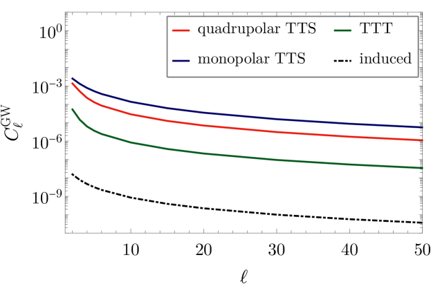
In Fig. 1 we plot the angular power spectra calculated in this section for a representative value |F~NLtts|=|FNLttt|=103subscriptsuperscript~𝐹ttsNLsubscriptsuperscript𝐹tttNLsuperscript103|\tilde{F}^{\text{tts}}_{\rm NL}|=|F^{\text{ttt}}_{\rm NL}|=10^{3} and taking r=0.05𝑟0.05r=0.05. As anticipated in Eq. (2.2), for |FNL|1much-greater-thansubscript𝐹NL1|F_{\rm NL}|\gg 1, we see that the angular power spectra for the intrinsic anisotropies are larger than the induced ones by roughly a factor (F~NLtts)2superscriptsubscriptsuperscript~𝐹ttsNL2(\tilde{F}^{\text{tts}}_{\rm NL})^{2} in the TTS case and r(FNLttt)2𝑟superscriptsubscriptsuperscript𝐹tttNL2r(F^{\text{ttt}}_{\rm NL})^{2} in the TTT case. Thus, for inflationary models with a significant enhancement of squeezed primordial non-Gaussianity, these anisotropies will be dominant.
Refer to caption
Figure 1: The auto-correlation of the SGWB anisotropies as a function of \ell plotted for |F~NLtts|=|FNLttt|=103subscriptsuperscript~𝐹ttsNLsubscriptsuperscript𝐹tttNLsuperscript103|\tilde{F}^{\text{tts}}_{\rm NL}|=|F^{\text{ttt}}_{\rm NL}|=10^{3} and the tensor-scalar ratio r=0.05𝑟0.05r=0.05.

3 CMB-GW Cross-correlation

The GW anisotropies considered in the previous section arise from the modulation of the primordial tensor power spectrum by the long wavelength scalar/tensor modes and will be correlated with the scalar/tensor contributions to the CMB temperature anisotropies δTsuperscript𝛿T\delta^{\rm{{T}}} 888One could also consider correlating the SGWB anisotropies with the E-mode polarisation of the CMB. Although this turns out to be smaller than the induced GW-T cross-correlation by at least one order of magnitude [49], including it can help put tighter constraints on F~NLttssubscriptsuperscript~𝐹ttsNL\tilde{F}^{\text{tts}}_{\rm NL}. As for the cross-correlation with CMB B-mode polarisation, this will be non-zero only when there is parity violation, similar to the CMB case where TB=0delimited-⟨⟩TB0\langle\rm TB\rangle=0 if parity is preserved in the theory.. Here, we calculate this cross-correlation and for the TTS case we comment briefly on the dependence of this cross-correlation on the angular structure of the primordial bispectrum. As in the previous section, we provide analytic estimates wherever possible by assuming a scale independent FNLsubscript𝐹NLF_{\rm NL} and Pζ(q)=(2π2/q3)ASsubscript𝑃𝜁𝑞2superscript𝜋2superscript𝑞3subscript𝐴𝑆P_{\zeta}(q)=(2\pi^{2}/q^{3})A_{S}.

3.1 Cross-correlations with induced anisotropies

Since the induced anisotropies are sourced by the large scale curvature perturbation, they are also correlated with the CMB temperature anisotropies. Their cross-correlation with the CMB is given by

δmGWδmT=δδmmCGWT,inddelimited-⟨⟩subscriptsuperscript𝛿GW𝑚subscriptsuperscript𝛿Tsuperscriptsuperscript𝑚subscript𝛿superscriptsubscript𝛿𝑚superscript𝑚superscriptsubscript𝐶GWTind\displaystyle\langle\delta^{\rm{{GW}}}_{\ell m}\delta^{\rm T*}_{\ell^{\prime}m^{\prime}}\rangle=\delta_{\ell\ell^{\prime}}\delta_{mm^{\prime}}C_{\ell}^{\rm{GW-T,ind}} (3.1)

with

CGWT,ind1615πq2𝑑qj(qd)j(qrlss)Pζ(q),similar-to-or-equalssuperscriptsubscript𝐶GWTind1615𝜋superscript𝑞2differential-d𝑞subscript𝑗𝑞𝑑subscript𝑗𝑞subscript𝑟lsssubscript𝑃𝜁𝑞\displaystyle C_{\ell}^{\rm{GW-T,ind}}\simeq\frac{16}{15\pi}\int q^{2}dq\,j_{\ell}(qd)j_{\ell}(qr_{\rm lss})P_{\zeta}(q)\,, (3.2)

assuming a flat spectrum for ΩGWsubscriptΩGW{\Omega_{{\rm{{GW}}}}}. To get to Eq. (3.2), we have assumed that the temperature anisotropies are given by the SW term which is a good approximation on large angular scales. Its spherical harmonic coefficients are given by [50],

δmT=4π5(i)d3p(2π)3Ym(p^)j(prlss)ζ(𝐩),subscriptsuperscript𝛿T𝑚4𝜋5superscript𝑖superscript𝑑3𝑝superscript2𝜋3subscriptsuperscript𝑌𝑚^𝑝subscript𝑗𝑝subscript𝑟lss𝜁𝐩\displaystyle\delta^{\rm{{T}}}_{\ell m}=\frac{4\pi}{5}(-i)^{\ell}\int\frac{d^{3}p}{(2\pi)^{3}}Y^{*}_{\ell m}(\hat{p})j_{\ell}(pr_{\rm lss})\zeta(\mathbf{p})\,, (3.3)

where rlsssubscript𝑟lssr_{\rm lss} denotes the comoving distance to the last scattering surface. Detailed numerical analyses of this cross-correlation highlighting the relative contribution of the various terms (SW, early and late ISW, Doppler etc.) and the effects of pre-recombination physics have been recently carried out in Refs. [51] and [49] respectively. For our purposes, it suffices to take only the SW term Eq. (3.3) since this is the main contribution to the cross-correlation (intrinsic as well as induced) on large angular scales. We can now evaluate this correlation analytically as

CGWT=32π15ASqkdqqj(qd)j(qrlss).subscriptsuperscript𝐶GWT32𝜋15subscript𝐴𝑆subscriptmuch-less-than𝑞𝑘𝑑𝑞𝑞subscript𝑗𝑞𝑑subscript𝑗𝑞subscript𝑟lss\displaystyle C^{\rm{GW-T}}_{\ell}=\frac{32\pi}{15}A_{S}\int_{q\ll k}\frac{dq}{q}\,j_{\ell}(qd)j_{\ell}(qr_{\rm lss})\,. (3.4)

For the low multipole range (<20)20(\ell<20), a good approximation can be obtained by letting d=rlss𝑑subscript𝑟lssd=r_{\rm lss} and using the identity Eq. (2.19) to get

CGWT32π15AS2(+1).similar-to-or-equalssubscriptsuperscript𝐶GWT32𝜋15subscript𝐴𝑆21\displaystyle C^{\rm{GW-T}}_{\ell}\simeq\frac{32\pi}{15}\frac{A_{S}}{2\ell(\ell+1)}\,. (3.5)

If instead one does not make this approximation, one can derive a more accurate but complicated expression in terms of the Gamma functions and the Hypergeometric function F12subscriptsubscript𝐹12{}_{2}F_{1} using the identity [46],

0𝑑xJν(ax)Jμ(bx)xλ=superscriptsubscript0differential-d𝑥subscript𝐽𝜈𝑎𝑥subscript𝐽𝜇𝑏𝑥superscript𝑥𝜆absent\displaystyle\int_{0}^{\infty}dx\,J_{\nu}(ax)J_{\mu}(bx)x^{-\lambda}= aνΓ(μ+νλ+12)2λbνλ+1Γ(μν+λ+12)Γ(ν+1)superscript𝑎𝜈Γ𝜇𝜈𝜆12superscript2𝜆superscript𝑏𝜈𝜆1Γ𝜇𝜈𝜆12Γ𝜈1\displaystyle\frac{a^{\nu}\,\Gamma(\frac{\mu+\nu-\lambda+1}{2})}{2^{\lambda}\,b^{\nu-\lambda+1}\Gamma(\frac{\mu-\nu+\lambda+1}{2})\Gamma(\nu+1)}
×F12(μ+νλ+12,νμλ+12;ν+1;a2b2),absentsubscriptsubscript𝐹12𝜇𝜈𝜆12𝜈𝜇𝜆12𝜈1superscript𝑎2superscript𝑏2\displaystyle\times{}_{2}F_{1}\left(\frac{\mu+\nu-\lambda+1}{2},\frac{\nu-\mu-\lambda+1}{2};\nu+1;\frac{a^{2}}{b^{2}}\right)\,, (3.6)
[for Re(μ+νλ+1)>0,Reλ>1, 0<a<b]delimited-[]formulae-sequencefor Re𝜇𝜈𝜆10formulae-sequenceRe𝜆1 0𝑎𝑏\displaystyle\left[\text{for }{\rm Re}\,{(\mu+\nu-\lambda+1)}>0,\;{\rm Re}\,{\lambda}>-1,\;0<a<b\right]

With this, from Eq. (3.4) we find

CGWT=8π3/215AS(rlssd)Γ()Γ(+32)F12(12,,+32,rlss2d2).subscriptsuperscript𝐶GWT8superscript𝜋3215subscript𝐴𝑆superscriptsubscript𝑟lss𝑑ΓΓ32subscriptsubscript𝐹121232superscriptsubscript𝑟lss2superscript𝑑2\displaystyle C^{\rm{GW-T}}_{\ell}=\frac{8\pi^{3/2}}{15}A_{S}\left(\frac{r_{\rm lss}}{d}\right)^{\ell}\frac{\Gamma(\ell)}{\Gamma(\ell+\frac{3}{2})}\;{}_{2}{F}_{1}\left(-\frac{1}{2},\ell,\ell+\frac{3}{2},\frac{r_{\rm lss}^{2}}{d^{2}}\right)\,. (3.7)

Thus we see that this cross-correlation decays sharply with \ell due to the factor (rlss/d)superscriptsubscript𝑟lss𝑑(r_{\rm lss}/d)^{\ell}, as also pointed out in Refs. [41, 51]. This suppression arises from the fact that the time when the gravitons begin their free streaming ηinsubscript𝜂in\eta_{\rm in} is different from that of the CMB photons ηlsssubscript𝜂lss\eta_{\rm lss}, thus rlss/d<1subscript𝑟lss𝑑1r_{\rm lss}/d<1 (recall that d=η0ηin𝑑subscript𝜂0subscript𝜂ind=\eta_{0}-\eta_{\rm in} for the short mode k𝑘k so ηinsubscript𝜂in\eta_{\rm in} corresponds to a conformal time deep within radiation domination, whereas rlss=η0ηlsssubscript𝑟lsssubscript𝜂0subscript𝜂lssr_{\rm lss}=\eta_{0}-\eta_{\rm lss}). As a result, these anisotropies become uncorrelated on small scales (large \ell). Since drlss𝑑subscript𝑟lssd\approx r_{\rm lss}, this also explains why the estimate of Eq. (3.5) works well for small \ell but fails for 20greater-than-or-equivalent-to20\ell\gtrsim 20 (see Figure 2). To see the explicit scaling with \ell we use the following numerical fit,

Γ()Γ(+32)F12(12,;+32;rlss2d2)0.8(+0.44)0.78similar-to-or-equalsΓΓ32subscriptsubscript𝐹121232superscriptsubscript𝑟lss2superscript𝑑20.8superscript0.440.78\displaystyle\frac{\Gamma(\ell)}{\Gamma(\ell+\frac{3}{2})}\,{}_{2}{F}_{1}\left(-\frac{1}{2},\ell;\ell+\frac{3}{2};\frac{r_{\rm lss}^{2}}{d^{2}}\right)\simeq\frac{0.8}{\ell(\ell+0.44)^{0.78}}\, (3.8)

which gives

CGWT,tts(rlssd)12.similar-tosubscriptsuperscript𝐶GWTttssuperscriptsubscript𝑟lss𝑑1superscript2\displaystyle C^{\rm{GW-T,tts}}_{\ell}\sim\left(\frac{r_{\rm lss}}{d}\right)^{\ell}\frac{1}{\ell^{2}}\,. (3.9)

A similar behaviour will also be present for the TTS cross-correlation, as we shall see below.

3.2 Cross-correlations with anisotropies from γγζdelimited-⟨⟩𝛾𝛾𝜁\langle\gamma\gamma\zeta\rangle bispectrum

Monopolar TTS

We consider here the CMB-GW cross-correlation for the intrinsic CGWB anisotropies where the long-wavelength mode is a scalar. For the monopolar F~NLttssubscriptsuperscript~𝐹ttsNL\tilde{F}^{\text{tts}}_{\rm NL} we have

CGWT=25πqkq2𝑑qj(qd)j(qrlss)F~NLtts(k,q)Pζ(q),subscriptsuperscript𝐶GWT25𝜋subscriptmuch-less-than𝑞𝑘superscript𝑞2differential-d𝑞subscript𝑗𝑞𝑑subscript𝑗𝑞subscript𝑟lsssubscriptsuperscript~𝐹ttsNL𝑘𝑞subscript𝑃𝜁𝑞\displaystyle C^{\rm{GW-T}}_{\ell}=\frac{2}{5\pi}\int_{q\ll k}q^{2}dq\,j_{\ell}(qd)j_{\ell}(qr_{\rm lss})\tilde{F}^{\text{tts}}_{\rm NL}(k,q)P_{\zeta}(q)\,, (3.10)

which was previously derived in [41]. Similar to the previous section, we can now analytically evaluate this cross-correlation,

CGWT=4π5F~NLttsASqkdqqj(qd)j(qrlss).subscriptsuperscript𝐶GWT4𝜋5subscriptsuperscript~𝐹ttsNLsubscript𝐴𝑆subscriptmuch-less-than𝑞𝑘𝑑𝑞𝑞subscript𝑗𝑞𝑑subscript𝑗𝑞subscript𝑟lss\displaystyle C^{\rm{GW-T}}_{\ell}=\frac{4\pi}{5}\tilde{F}^{\text{tts}}_{\rm NL}A_{S}\int_{q\ll k}\frac{dq}{q}\,j_{\ell}(qd)j_{\ell}(qr_{\rm lss})\,. (3.11)

The approximation with d=rlss𝑑subscript𝑟lssd=r_{\rm lss} gives

CGWT4π5F~NLttsAS2(+1).similar-to-or-equalssubscriptsuperscript𝐶GWT4𝜋5subscriptsuperscript~𝐹ttsNLsubscript𝐴𝑆21\displaystyle C^{\rm{GW-T}}_{\ell}\simeq\frac{4\pi}{5}\tilde{F}^{\text{tts}}_{\rm NL}\frac{A_{S}}{2\ell(\ell+1)}\,. (3.12)

The full result with drlss𝑑subscript𝑟lssd\neq r_{\rm lss} and using Eq. (3.1) is instead

CGWT=π3/25F~NLttsAS(rlssd)Γ()Γ(+32)F12(12,;+32;rlss2d2).subscriptsuperscript𝐶GWTsuperscript𝜋325subscriptsuperscript~𝐹ttsNLsubscript𝐴𝑆superscriptsubscript𝑟lss𝑑ΓΓ32subscriptsubscript𝐹121232superscriptsubscript𝑟lss2superscript𝑑2\displaystyle C^{\rm{GW-T}}_{\ell}=\frac{\pi^{3/2}}{5}\tilde{F}^{\text{tts}}_{\rm NL}A_{S}\left(\frac{r_{\rm lss}}{d}\right)^{\ell}\frac{\Gamma(\ell)}{\Gamma(\ell+\frac{3}{2})}\,{}_{2}{F}_{1}\left(-\frac{1}{2},\ell;\ell+\frac{3}{2};\frac{r_{\rm lss}^{2}}{d^{2}}\right)\,. (3.13)

We see that the cross-correlation for the monopolar TTS scales with \ell in exactly the same manner as the cross-correlation for the induced anisotropies,

CGWT,tts=(38F~NLtts)CGWT,ind.subscriptsuperscript𝐶GWTtts38subscriptsuperscript~𝐹ttsNLsuperscriptsubscript𝐶GWTind\displaystyle C^{\rm{GW-T,tts}}_{\ell}=\left(\frac{3}{8}\tilde{F}^{\text{tts}}_{\rm NL}\right)C_{\ell}^{\rm{GW-T,ind}}\,. (3.14)

Quadrupolar TTS

For the quadrupolar case we have,

CGWT,tts=4πLiLh2L2GL2+1,subscriptsuperscript𝐶GWTtts4𝜋subscript𝐿superscript𝑖𝐿superscriptsubscript2𝐿2subscript𝐺𝐿21\displaystyle C^{\rm{GW-T,tts}}_{\ell}=4\pi\sum_{L}i^{L-\ell}h_{2L\ell}^{2}\frac{G_{L\ell}}{2\ell+1}\,, (3.15)

where the sum is over L=2,,+2𝐿22L=\ell-2,\ell,\ell+2 and the function G12subscript𝐺subscript1subscript2G_{\ell_{1}\ell_{2}} is defined as

G12subscript𝐺subscript1subscript2\displaystyle G_{\ell_{1}\ell_{2}} =225πqkq2𝑑qj1(qd)j2(qrlss)F~NLtts(k,q)Pζ(q),absent225𝜋subscriptmuch-less-than𝑞𝑘superscript𝑞2differential-d𝑞subscript𝑗subscript1𝑞𝑑subscript𝑗subscript2𝑞subscript𝑟lsssubscriptsuperscript~𝐹ttsNL𝑘𝑞subscript𝑃𝜁𝑞\displaystyle=\frac{2}{25\pi}\int_{q\ll k}q^{2}dq\,j_{\ell_{1}}(qd)j_{\ell_{2}}(qr_{\rm lss})\tilde{F}^{\text{tts}}_{\rm NL}(k,q)P_{\zeta}(q), (3.16)

and h123subscriptsubscript1subscript2subscript3h_{\ell_{1}\ell_{2}\ell_{3}} was defined in Eq. (2.27). The result Eq. (3.15), previously derived in [44], can now be analytically estimated using Eq. (3.1) to get

CGWT,tts=π3/2F~NLttsAS20(rlssd)(rlssd1)(rlssd+1)ΔF,subscriptsuperscript𝐶GWTttssuperscript𝜋32subscriptsuperscript~𝐹ttsNLsubscript𝐴𝑆20superscriptsubscript𝑟lss𝑑subscript𝑟lss𝑑1subscript𝑟lss𝑑1Δsubscript𝐹\displaystyle C^{\rm{GW-T,tts}}_{\ell}=\frac{\pi^{3/2}\tilde{F}^{\text{tts}}_{\rm NL}A_{S}}{20}\left(\frac{r_{\rm lss}}{d}\right)^{\ell}\left(\frac{r_{\rm lss}}{d}-1\right)\left(\frac{r_{\rm lss}}{d}+1\right)\Delta F_{\ell}\,, (3.17)

where ΔFΔsubscript𝐹\Delta F_{\ell} is given by

ΔFΓ()Γ(+3/2)[(+1)F12(12,;+32;rlss2d2)F12(12,;+32;rlss2d2)].Δsubscript𝐹ΓΓ32delimited-[]1subscriptsubscript𝐹121232superscriptsubscript𝑟lss2superscript𝑑2subscriptsubscript𝐹121232superscriptsubscript𝑟lss2superscript𝑑2\displaystyle\Delta F_{\ell}\equiv\frac{\Gamma(\ell)}{\Gamma(\ell+3/2)}\left[(\ell+1)\,{}_{2}{F}_{1}\left(-\frac{1}{2},\ell;\ell+\frac{3}{2};\frac{r_{\text{lss}}^{2}}{d^{2}}\right)-\,{}_{2}{F}_{1}\left(\frac{1}{2},\ell;\ell+\frac{3}{2};\frac{r_{\text{lss}}^{2}}{d^{2}}\right)\right]\,. (3.18)

The function ΔFΔsubscript𝐹\Delta F_{\ell} is well fit by

ΔF0.2(+2)0.45.similar-to-or-equalsΔsubscript𝐹0.2superscript20.45\displaystyle\Delta F_{\ell}\simeq\frac{0.2}{(\ell+2)^{0.45}}\,. (3.19)

Thus, the CGWT,ttssubscriptsuperscript𝐶GWTttsC^{\rm{GW-T,tts}}_{\ell} for the quadrupolar case scales with \ell as

CGWT,tts(rlssd)11/2.similar-tosubscriptsuperscript𝐶GWTttssuperscriptsubscript𝑟lss𝑑1superscript12\displaystyle C^{\rm{GW-T,tts}}_{\ell}\sim\left(\frac{r_{\rm lss}}{d}\right)^{\ell}\frac{1}{\ell^{1/2}}\,. (3.20)

From the above results we notice the familiar (rlss/d)superscriptsubscript𝑟lss𝑑(r_{\rm lss}/d)^{\ell} suppression that we have seen previously in Eq. (3.7) and Eq. (3.13) for the induced and monopolar TTS anisotropies, thus the cross-correlation again decreases as we go towards the smaller scales. However from Eq. (3.17), we also see that for the quadrupolar case when drlss𝑑subscript𝑟lssd\to r_{\rm lss}, this cross-correlation does not increase, instead it drops to zero. Physically, this can be understood from the fact that the source term for the GW anisotropy is locally a quadrupole, whereas the source term for the CMB is a monopole. Therefore, if the sources operate at the same point in space, their cross-correlation will be zero (orthogonality of the Legendre polynomials 𝒫(k^q^)subscript𝒫^𝑘^𝑞\mathcal{P}_{\ell}(\hat{k}\cdot\hat{q}) and 𝒫(k^q^)subscript𝒫superscript^𝑘^𝑞\mathcal{P}_{\ell^{\prime}}(\hat{k}\cdot\hat{q}) for superscript\ell\neq\ell^{\prime}). A further point of difference is that this cross-correlation decays more slowly compared to the monopolar one owing to the term proportional to (+1)1(\ell+1) in ΔFΔsubscript𝐹\Delta F_{\ell}.

Refer to caption
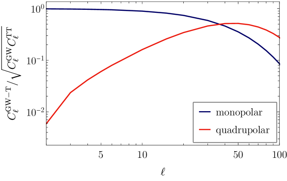
Figure 2: The ratio CGWT/CGWCTTsubscriptsuperscript𝐶GWTsubscriptsuperscript𝐶GWsubscriptsuperscript𝐶TTC^{\rm{GW-T}}_{\ell}/\sqrt{C^{\rm{GW}}_{\ell}C^{\rm{TT}}_{\ell}} plotted for the monopolar and the quadrupolar TTS cross-correlation. The corresponding ratio for the induced anisotropies follows the same curve as the one for the monopolar TTS.

Overall, from the results of this section one can expect that the cross-correlation for the quadrupolar TTS will be smaller compared to the one for the monopolar TTS which will have important consequences for cross-correlation-based observations/constraints on CGWB anisotropies. We can understand why this is to be expected by looking at the expression for the relative error in estimating the individual CGWTsubscriptsuperscript𝐶GWTC^{\rm{GW-T}}_{\ell} (e.g. see [52]),

δCGWT[CTTCGW(2+1)(CGWT)2]1/2.proportional-to𝛿subscriptsuperscript𝐶GWTsuperscriptdelimited-[]subscriptsuperscript𝐶TTsubscriptsuperscript𝐶GW21superscriptsubscriptsuperscript𝐶GWT212\displaystyle\delta C^{\rm{GW-T}}_{\ell}\propto\left[{\frac{C^{\rm{TT}}_{\ell}C^{\rm{GW}}_{\ell}}{(2\ell+1)(C^{\rm{GW-T}}_{\ell})^{2}}}\right]^{1/2}\,. (3.21)

The ratio CGWT/CGWCTTsubscriptsuperscript𝐶GWTsubscriptsuperscript𝐶GWsubscriptsuperscript𝐶TTC^{\rm{GW-T}}_{\ell}/\sqrt{C^{\rm{GW}}_{\ell}C^{\rm{TT}}_{\ell}} is plotted in Fig. 2 for the monopolar and the quadrupolar cross-correlations. In the low \ell range which is the relevant range for GW detectors999Even though the ratio CGWT/CGWCTTsubscriptsuperscript𝐶GWTsubscriptsuperscript𝐶GWsubscriptsuperscript𝐶TTC^{\rm{GW-T}}_{\ell}/\sqrt{C^{\rm{GW}}_{\ell}C^{\rm{TT}}_{\ell}} increases initially for the quadrupolar case, higher multipoles do not offer any improvement on the constraints. This is due to the fact that the angular resolution of GW detectors is quite poor and we typically have CGWNGWsimilar-to-or-equalssubscriptsuperscript𝐶GWsubscriptsuperscript𝑁GWC^{\rm{GW}}_{\ell}\simeq N^{\rm{GW}}_{\ell}, i.e. a noise dominated map with the NGWsuperscriptsubscript𝑁GWN_{\ell}^{\text{\tiny GW}} increasing quite rapidly with \ell whereas the signal typically decreases. Thus, in practice one is limited to max1530similar-tosubscriptmax1530\ell_{\rm max}\sim 15\text{--}30 (e.g. see [53, 54] for ground-based networks and LISA, and see Fig. 3 for other examples)., we have (CGWT)2CGWCTTsimilar-to-or-equalssuperscriptsubscriptsuperscript𝐶GWT2subscriptsuperscript𝐶GWsubscriptsuperscript𝐶TT(C^{\rm{GW-T}}_{\ell})^{2}\simeq C^{\rm{GW}}_{\ell}C^{\rm{TT}}_{\ell} for the monopolar TTS, whereas for the quadrupolar case we have (CGWT)2CGWCTTmuch-less-thansuperscriptsubscriptsuperscript𝐶GWT2subscriptsuperscript𝐶GWsubscriptsuperscript𝐶TT(C^{\rm{GW-T}}_{\ell})^{2}\ll C^{\rm{GW}}_{\ell}C^{\rm{TT}}_{\ell}. Thus, based on the above considerations, we expect cross-correlations to be more effective in the case of the monopolar TTS as compared to the quadrupolar TTS. We confirm this in the following section.

3.2.1 Projected constraints on F~NLttssubscriptsuperscript~𝐹ttsNL\tilde{F}^{\text{tts}}_{\rm NL}

We now estimate the error in the measurement of F~NLttssubscriptsuperscript~𝐹ttsNL\tilde{F}^{\text{tts}}_{\rm NL} using a joint auto- and cross-correlation measurement. The Fisher matrix in this case is given by [55, 44],

Fij=XY=minmaxCXθi(𝒞XY)1CYθj,subscript𝐹𝑖𝑗subscript𝑋𝑌superscriptsubscriptsubscriptminsubscriptmaxsubscriptsuperscript𝐶𝑋subscript𝜃𝑖superscriptsuperscriptsubscript𝒞𝑋𝑌1subscriptsuperscript𝐶𝑌subscript𝜃𝑗\displaystyle F_{ij}=\sum_{XY}\sum_{{\ell=}\ell_{\rm min}}^{\ell_{\rm max}}\frac{\partial C^{X}_{\ell}}{\partial\theta_{i}}\left(\mathscr{C}_{\ell}^{XY}\right)^{-1}\frac{\partial C^{Y}_{\ell}}{\partial\theta_{j}}\,, (3.22)

where X,Y={TT,GW,GW-T}𝑋𝑌TT,GW,GW-TX,Y=\{{\text{TT,GW,GW-T}}\} and θisubscript𝜃𝑖\vec{\theta}_{i} are the parameters being measured. The elements of the matrix 𝒞subscript𝒞\mathscr{C}_{\ell} are

𝒞=22+1[(CTT)2(CGWT)2CTTCGWT(CGWT)2(CGW)2CGWCGWTCTTCGWTCGWCGWT12(CGWT)2+12CTTCGW].subscript𝒞221matrixsuperscriptsubscriptsuperscript𝐶TT2superscriptsubscriptsuperscript𝐶GWT2subscriptsuperscript𝐶TTsubscriptsuperscript𝐶GWTsuperscriptsubscriptsuperscript𝐶GWT2superscriptsubscriptsuperscript𝐶GW2subscriptsuperscript𝐶GWsubscriptsuperscript𝐶GWTsubscriptsuperscript𝐶TTsubscriptsuperscript𝐶GWTsubscriptsuperscript𝐶GWsubscriptsuperscript𝐶GWT12superscriptsubscriptsuperscript𝐶GWT212subscriptsuperscript𝐶TTsubscriptsuperscript𝐶GW\displaystyle\mathscr{C}_{\ell}=\frac{2}{2\ell+1}\begin{bmatrix}(C^{\rm{TT}}_{\ell})^{2}&(C^{\rm{GW-T}}_{\ell})^{2}&C^{\rm{TT}}_{\ell}C^{\rm{GW-T}}_{\ell}\\ (C^{\rm{GW-T}}_{\ell})^{2}&(C^{\rm{GW}}_{\ell})^{2}&C^{\rm{GW}}_{\ell}C^{\rm{GW-T}}_{\ell}\\ C^{\rm{TT}}_{\ell}C^{\rm{GW-T}}_{\ell}&C^{\rm{GW}}_{\ell}C^{\rm{GW-T}}_{\ell}&\frac{1}{2}(C^{\rm{GW-T}}_{\ell})^{2}+\frac{1}{2}C^{\rm{TT}}_{\ell}C^{\rm{GW}}_{\ell}\end{bmatrix}\,. (3.23)

The error is then estimated as Δθi=(F1)iiΔsubscript𝜃𝑖subscriptsuperscript𝐹1𝑖𝑖\Delta\theta_{i}=\sqrt{(F^{-1})_{ii}} with

CTTsubscriptsuperscript𝐶TT\displaystyle C^{\rm{TT}}_{\ell} 2πAS25(+1),similar-to-or-equalsabsent2𝜋subscript𝐴𝑆251\displaystyle\simeq\frac{2\pi A_{S}}{25\ell(\ell+1)},
CGWsubscriptsuperscript𝐶GW\displaystyle C^{\rm{GW}}_{\ell} =CGW,tts+CGW,ind+NGW,absentsubscriptsuperscript𝐶GWttssuperscriptsubscript𝐶GWindsubscriptsuperscript𝑁GW\displaystyle=C^{\rm{GW,tts}}_{\ell}+C_{\ell}^{\rm{GW,ind}}+N^{\rm{GW}}_{\ell}, (3.24)
CGWTsubscriptsuperscript𝐶GWT\displaystyle C^{\rm{GW-T}}_{\ell} =CGWT,tts+CGWT,ind,absentsubscriptsuperscript𝐶GWTttssuperscriptsubscript𝐶GWTind\displaystyle=C^{\rm{GW-T,tts}}_{\ell}+C_{\ell}^{\rm{GW-T,ind}},

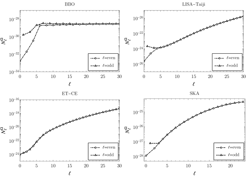
with the NGWsuperscriptsubscript𝑁GWN_{\ell}^{\text{\tiny GW}} being the noise angular power spectra of the detector network being used for the measurement (Fig. 3).
Refer to caption
Figure 3: NΩsuperscriptsubscript𝑁ΩN_{\ell}^{\Omega} plotted for BBO, LISA-Taiji, ET-CE and SKA at frefBBO=0.1superscriptsubscript𝑓refBBO0.1f_{\rm ref}^{\rm BBO}=0.1 Hz, frefLISATaiji=0.01superscriptsubscript𝑓refLISATaiji0.01f_{\rm ref}^{\rm LISA-Taiji}=0.01 Hz, frefETCE=63superscriptsubscript𝑓refETCE63f_{\rm ref}^{\rm ET-CE}=63 Hz and frefSKA=1year1superscriptsubscript𝑓refSKA1superscriptyear1f_{\rm ref}^{\rm SKA}=1\,{\rm year}^{-1} Hz. The quantity NGWsuperscriptsubscript𝑁GWN_{\ell}^{\rm GW} is defined as NGWNΩ/Ω¯GW2superscriptsubscript𝑁GWsuperscriptsubscript𝑁Ωsubscriptsuperscript¯Ω2GWN_{\ell}^{\rm GW}\equiv N_{\ell}^{\Omega}/\overline{\Omega}^{2}_{\rm GW}

The calculation of the NGWsuperscriptsubscript𝑁GWN_{\ell}^{\rm GW} is based on the formalism of [54] and employs the associated code schNell101010https://github.com/damonge/schNell. The NGWsuperscriptsubscript𝑁GWN_{\ell}^{\rm GW} for ET-CE were already calculated in [54] and following [44] we have adapted this code to calculate the NGWsuperscriptsubscript𝑁GWN_{\ell}^{\rm GW} for BBO, LISA-Taiji and SKA. The details of their detector configurations and noise curves are described below.

BBO

We consider the full BBO configuration with 4 LISA-like constellations, 2 of which will be arranged as a six-pointed star. In addition there will be 2 outer constellations trailing and leading the star constellation by 120superscript120120^{\circ} in an earth-like orbit around the sun [56]. The full BBO configuration improves upon the star configuration by reducing the noise at the >44\ell>4 multipoles (compare to Fig. 5 of [44]). The noise curve for BBO is given in Ref. [57] and the total time of observation is taken to be Tobs=4subscript𝑇obs4T_{\rm obs}=4 years.

LISA-Taiji

The total time of observation is taken to be Tobs=4subscript𝑇obs4T_{\rm obs}=4 years and the noise curves for LISA and Taiji are obtained from [58] and [59] respectively. Both LISA and Taiji will be in an earth-like orbit around the sun with an angular separation of 40superscript4040^{\circ} [59].

ET-CE

The total time of observation is taken to be Tobs=4subscript𝑇obs4T_{\rm obs}=4 years and the noise curves for ET111111http://www.et-gw.eu/index.php and CE121212https://dcc.ligo.org/LIGO-T1500293/public are also available online. The locations for ET and CE are taken to be the same as those assumed in [54].

PTAs

We consider a futuristic PTA experiment like SKA with a network of Npsrsubscript𝑁psrN_{\rm psr} identical pulsars distributed isotropically across the sky whose timing noise is of the form [60],

Nf=2σt2ΔT.subscript𝑁𝑓2superscriptsubscript𝜎𝑡2Δ𝑇\displaystyle N_{f}=2\sigma_{t}^{2}\Delta T\,. (3.25)

Here 1/ΔT1Δ𝑇1/\Delta T is the cadence of the observations and σtsubscript𝜎𝑡\sigma_{t} is the rms error of the timing residuals. For SKA we assume the following set of values Npsr=50subscript𝑁psr50N_{\rm psr}=50, ΔT=2Δ𝑇2\Delta T=2 weeks, σt=30subscript𝜎𝑡30\sigma_{t}=30 ns and a total time of observation Tobs=20subscript𝑇obs20T_{\rm obs}=20 years. The choice of values is similar to that considered in [61]. This estimate for the NGWsuperscriptsubscript𝑁GWN_{\ell}^{\rm GW} could be made more realistic by dropping the assumption of identical pulsars and including additional sources of noise, e.g. a red timing noise as well as correlated noise sources arising from clock or solar system ephemeris errors [62]. One could also consider including more pulsars (Npsr1001000similar-tosubscript𝑁psr1001000N_{\rm psr}\sim 100\operatorname{--}1000), as expected for SKA2 [63]. We leave this for future work.

In Fig. 4 we plot the relative error in the measurement of F~NLttssubscriptsuperscript~𝐹ttsNL\tilde{F}^{\text{tts}}_{\rm NL} defined as

δF~NLttsΔF~NLtts/F~NLtts,𝛿subscriptsuperscript~𝐹ttsNLΔsubscriptsuperscript~𝐹ttsNLsubscriptsuperscript~𝐹ttsNL\displaystyle\delta\tilde{F}^{\text{tts}}_{\rm NL}\equiv{\Delta\tilde{F}^{\text{tts}}_{\rm NL}}/{\tilde{F}^{\text{tts}}_{\rm NL}}\,, (3.26)

for different values of ΩGWsubscriptΩGW{\Omega_{{\rm{{GW}}}}} and taking a scale independent F~NLtts=103subscriptsuperscript~𝐹ttsNLsuperscript103\tilde{F}^{\text{tts}}_{\rm NL}=10^{3}.

Refer to caption
Refer to caption
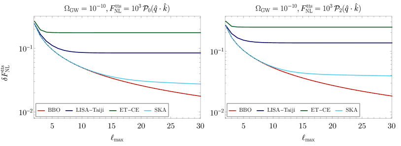
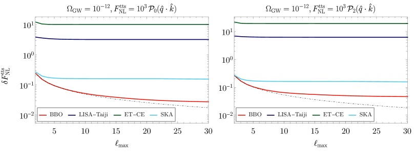
Figure 4: The relative error in the measurement of F~NLttssubscriptsuperscript~𝐹ttsNL\tilde{F}^{\text{tts}}_{\rm NL} as a function of maxsubscriptmax\ell_{\rm max} for BBO, SKA, LISA-Taiji and ET-CE. The dashed curves show the errors for an idealised, cosmic variance limited measurement.

In calculating the error we have also assumed for simplicity a spectrum for ΩGWsubscriptΩGW{\Omega_{{\rm{{GW}}}}} that is flat on small scales, in the frequency range relevant to the particular GW detector. For reference, note that we previously defined

FNLtts(𝐤,𝐪)=F~NLtts𝒫(q^k^)subscriptsuperscript𝐹ttsNL𝐤𝐪subscriptsuperscript~𝐹ttsNLsubscript𝒫^𝑞^𝑘\displaystyle F^{\text{tts}}_{\rm NL}(\mathbf{k},\mathbf{q})=\tilde{F}^{\text{tts}}_{\rm NL}\,\mathcal{P}_{\ell}(\hat{q}\cdot\hat{k}) (3.27)

in terms of the Legendre polynomials with =0,202\ell=0,2 for the monopolar and quadrupolar cases respectively. We see that for a large value of the CGWB monopole ΩGW=1010subscriptΩGWsuperscript1010{\Omega_{{\rm{{GW}}}}}=10^{-10} we can achieve a relative error δF~NLtts102similar-to-or-equals𝛿superscriptsubscript~𝐹NLttssuperscript102\delta\tilde{F}_{\rm NL}^{\rm tts}\simeq 10^{-2} with BBO for both the monopolar and the quadrupolar FNLttssubscriptsuperscript𝐹ttsNLF^{\text{tts}}_{\rm NL} and a slightly larger error with SKA. With the ET-CE and LISA-Taiji networks the relative error in this case is of the order 101superscript10110^{-1} and saturates quickly around max10similar-tosubscriptmax10\ell_{\rm max}\sim 10 due to their lower sensitivity compared to BBO. For a smaller value of ΩGW=1012subscriptΩGWsuperscript1012{\Omega_{{\rm{{GW}}}}}=10^{-12} only BBO and SKA are able to detect FNLttssubscriptsuperscript𝐹ttsNLF^{\text{tts}}_{\rm NL}, reaching a relative error of the order 101superscript10110^{-1}. For both values of ΩGWsubscriptΩGW{\Omega_{{\rm{{GW}}}}} BBO is cosmic variance limited, especially for the monopolar TTS. We also see that the error is smaller in the case of the monopolar TTS as compared to the quadrupolar one, which is to be expected from the discussion of the previous section.

Astrophysical foregrounds

The analysis carried out so far implicitly assumes that only the cosmological background contributes to the SGWB. However, in addition to this background, one also expects a background of gravitational waves arising from unresolved astrophysical sources to contribute to the SGWB and its anisotropies [64, 65, 66, 67, 68, 69, 70, 71, 72, 73, 74, 75, 76]. Detecting the cosmological background in the presence of this astrophysical foreground will be a major challenge and various methods to separate the monopoles of these backgrounds have been proposed in [77, 78, 79, 80, 81, 82, 83, 84, 85]. Importantly, these techniques exploit the fact that astrophysical and cosmological backgrounds have different properties w.r.t their frequency range, spectral dependence, yearly modulation (e.g. in the case of galactic binaries), and can thus be distinguished from each other. In particular for the inflationary background, there is the possibility of detection on vastly different scales ranging from the CMB up to interferometers whereas the various different astrophysical backgrounds are each expected to be limited to a much smaller frequency window.
Moving beyond the monopole, one can also study the prospects of detecting the anisotropies of such backgrounds, both cosmological and astrophysical. Since the properties of the astrophysical background depend strongly on the distribution of the large scale structure, it will have cross-correlations with probes like galaxy clustering and weak lensing [65, 67, 86, 87, 88, 89]. As for cross-correlation of the AGWB anisotropies with the CMB, this is a direction which is being actively investigated [51]. Interestingly, the findings of [51] suggest that cross-correlating the CMB with the cosmological SGWB provides a stronger signal131313A GW signal of cosmological origin that is detectable at e.g. BBO frequencies is assumed here.. One may then exploit these cross-correlations to help distinguish between astrophysical and primordial anisotropies.

To highlight the effectiveness of this approach, we compute here the signal to noise ratio of the cross-correlation of the primordial GW anisotropies with the CMB in the presence of an astrophysical background which acts as a foreground to the primordial signal. The signal to noise ratio (SNR) of this cross-correlation is defined as

SNR×=[minmax(2+1)(CGWT,signal)2(CGWT,total)2+CGW,totalCTT]1/2,superscriptSNRsuperscriptdelimited-[]superscriptsubscriptsubscriptminsubscriptmax21superscriptsuperscriptsubscriptCGWTsignal2superscriptsuperscriptsubscriptCGWTtotal2superscriptsubscriptCGWtotalsubscriptsuperscriptCTT12\displaystyle\rm{SNR}^{\times}=\left[\sum_{\ell_{\rm min}}^{\ell_{\rm max}}(2\ell+1)\frac{\left(C_{\ell}^{\rm{GW-T,signal}}\right)^{2}}{\left(C_{\ell}^{\rm{GW-T,total}}\right)^{2}+C_{\ell}^{\rm{GW,total}}C^{\rm{TT}}_{\ell}}\right]^{1/2}\,, (3.28)

where

CGWT,signal=CGWT,ttssuperscriptsubscript𝐶GWTsignalsubscriptsuperscript𝐶GWTtts\displaystyle C_{\ell}^{\rm{GW-T,signal}}=C^{\rm{GW-T,tts}}_{\ell}\,
CGWT,total=CGWT,signal+CGWT,induced,superscriptsubscript𝐶GWTtotalsuperscriptsubscript𝐶GWTsignalsuperscriptsubscript𝐶GWTinduced\displaystyle C_{\ell}^{\rm{GW-T,total}}=C_{\ell}^{\rm{GW-T,signal}}+C_{\ell}^{\rm{GW-T,induced}}\,, (3.29)
CGW,total=CGW,tts+CGW,induced+CGW,astro+NGW.superscriptsubscript𝐶GWtotalsuperscriptsubscript𝐶GWttssuperscriptsubscript𝐶GWinducedsuperscriptsubscript𝐶GWastrosuperscriptsubscript𝑁GW\displaystyle C_{\ell}^{\rm{GW,total}}=C_{\ell}^{\rm{GW,tts}}+C_{\ell}^{\rm{GW,induced}}+C_{\ell}^{\rm{GW,astro}}+N_{\ell}^{\rm GW}\,.

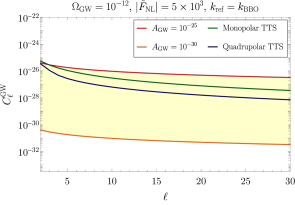
We assume an astrophysical background of the form (+1/2)CGW,astroAGWB12superscriptsubscript𝐶GWastrosubscript𝐴GWB(\ell+1/2)C_{\ell}^{\rm{GW,astro}}\approx A_{\rm GWB}, which is based on the astrophysical models of [67, 68, 69]. The upper limit AGWB=1025subscript𝐴GWBsuperscript1025A_{\rm GWB}=10^{-25} roughly corresponds to the expected magnitude of the background around f=63𝑓63f=63 Hz, while the lower limit AGWB=1030subscript𝐴GWBsuperscript1030A_{\rm GWB}=10^{-30} corresponds to the magnitude around f=0.01𝑓0.01f=0.01 Hz [68, 69]. Since our aim here is to estimate the SNR for the cross-correlation at the frequency range relevant to BBO, we assume for simplicity that the quantity AGWBsubscript𝐴GWBA_{\rm GWB} takes on values between these two limits.
Refer to caption
Figure 5: The CGWsubscriptsuperscript𝐶GWC^{\rm{GW}}_{\ell} for the astrophysical background (yellow shaded region) and for the CGWB with ΩGW=1012,|F~NLtts|=5×10³formulae-sequencesubscriptΩGWsuperscript1012subscriptsuperscript~𝐹ttsNL5superscript103{\Omega_{{\rm{{GW}}}}}=10^{-12},|\tilde{F}^{\text{tts}}_{\rm NL}|=5\times 10^{3}. We have assumed an astrophysical background of the form (+1/2)C=AGWB12subscript𝐶subscript𝐴GWB(\ell+1/2)C_{\ell}=A_{\rm GWB}. For comparison the CGWsubscriptsuperscript𝐶GWC^{\rm{GW}}_{\ell} of the CGWB have been rescaled as CGWΩ¯GW2CGWsubscriptsuperscript𝐶GWsuperscriptsubscript¯ΩGW2subscriptsuperscript𝐶GWC^{\rm{GW}}_{\ell}\to\overline{\Omega}_{\text{\tiny GW}}^{2}C^{\rm{GW}}_{\ell}.

The resulting SNR is plotted in Fig. 6. As discussed earlier in this section, the SNR for the monopolar TTS cross-correlation is much larger than that of the quadrupolar TTS. The primordial signal can be detected at a statistically significant level even for the upper limit of the astrophysical background, AGWB=1025subscript𝐴GWBsuperscript1025A_{\rm GWB}=10^{-25}, despite the fact this upper limit is larger than the primordial CGWsubscriptsuperscript𝐶GWC^{\rm{GW}}_{\ell} whenever ΩGW<1012subscriptΩGWsuperscript1012{\Omega_{{\rm{{GW}}}}}<10^{-12} and |F~NLtts|<5×10³subscriptsuperscript~𝐹ttsNL5superscript103|\tilde{F}^{\text{tts}}_{\rm NL}|<5\times 10^{3} (see Fig. 5). Thus, even if a direct observation of the primordial anisotropies is made difficult by the presence of the astrophysical foreground, cross-correlations with the CMB can still prove to be useful. We also see that for the quadrupolar TTS, a similar SNR is possible for a much weaker astrophysical signal, with AGWB=1027subscript𝐴GWBsuperscript1027A_{\rm GWB}=10^{-27} or lower.

Refer to caption
Refer to caption
Figure 6: Left : SNR for the GW-CMB cross-correlation arising from the monopolar TTS bispectrum plotted as a function of ΩGWsubscriptΩGW{\Omega_{{\rm{{GW}}}}} and |F~NLtts|subscriptsuperscript~𝐹ttsNL|\tilde{F}^{\text{tts}}_{\rm NL}|, taking (+1/2)C=AGWB12subscript𝐶subscript𝐴GWB(\ell+1/2)C_{\ell}=A_{\rm GWB} for the astrophysical background. Right: SNR for the same cross-correlation but for the quadrupolar TTS bispectrum.

3.3 Cross-correlations with anisotropies from γγγdelimited-⟨⟩𝛾𝛾𝛾\langle\gamma\gamma\gamma\rangle bispectrum

We now calculate the cross-correlation of the intrinsic GW anisotropies from the TTT bispectrum, Eq. (2.14), with the CMB temperature anisotropies sourced by the large scale tensor modes. This contribution to the CMB temperature anisotropies can be written as [48],

δT(n^)=12s=±2𝑑ηd3q(2π)3γ𝐪sηϵijs(q^)n^in^jeiχ(η)n^𝐪,superscript𝛿T^𝑛12subscript𝑠plus-or-minus2differential-d𝜂superscript𝑑3𝑞superscript2𝜋3subscriptsuperscript𝛾𝑠𝐪𝜂superscriptsubscriptitalic-ϵ𝑖𝑗𝑠^𝑞superscript^𝑛𝑖superscript^𝑛𝑗superscript𝑒𝑖𝜒𝜂^𝑛𝐪\displaystyle\delta^{\rm{{T}}}(\hat{n})=-\frac{1}{2}\sum_{s=\pm 2}\int\,d\eta\,\frac{d^{3}q}{\left(2\pi\right)^{3}}\frac{\partial\gamma^{s}_{\mathbf{q}}}{\partial\eta}\epsilon_{ij}^{s}(\hat{q})\hat{n}^{i}\hat{n}^{j}e^{-i\chi(\eta)\hat{n}\cdot\mathbf{q}}\,, (3.30)

where χ(η)=η0η𝜒𝜂subscript𝜂0𝜂\chi(\eta)=\eta_{0}-\eta and the integral over the conformal time spans from ηi=ηrecsubscript𝜂𝑖subscript𝜂rec\eta_{i}=\eta_{\rm rec} to ηf=η0subscript𝜂𝑓subscript𝜂0\eta_{f}=\eta_{0}. The spherical harmonic coefficients can be obtained using Eq. (2.32),

δmT=π(i)(+2)!(2)!s=±2𝑑ηd3q(2π)3γ𝐪sηj(qχ(η))(qχ(η))2YLMs(q^).subscriptsuperscript𝛿T𝑚𝜋superscript𝑖22subscript𝑠plus-or-minus2differential-d𝜂superscript𝑑3𝑞superscript2𝜋3subscriptsuperscript𝛾𝑠𝐪𝜂subscript𝑗𝑞𝜒𝜂superscript𝑞𝜒𝜂2subscriptsuperscriptsubscript𝑌𝐿𝑀𝑠^𝑞\displaystyle\delta^{\rm{{T}}}_{\ell m}=\pi\,(-i)^{\ell}\sqrt{\frac{(\ell+2)!}{(\ell-2)!}}\sum_{s=\pm 2}\int\,d\eta\,\frac{d^{3}q}{\left(2\pi\right)^{3}}\frac{\partial\gamma^{s}_{\mathbf{q}}}{\partial\eta}\frac{j_{\ell}(q\chi(\eta))}{(q\chi(\eta))^{2}}{}_{-s}Y_{LM}^{*}(\hat{q})\,. (3.31)

The resulting cross-correlation is

CGWT,ttt=(1)(+1)(+2)4πsubscriptsuperscript𝐶GWTttt1124𝜋\displaystyle C^{\rm{GW-T,ttt}}_{\ell}=\frac{(\ell-1)\ell(\ell+1)(\ell+2)}{4\pi} s=±2qkq2𝑑qFNLttt(𝐤,𝐪)Pγs(q)j(qd)(qd)2subscript𝑠plus-or-minus2subscriptmuch-less-than𝑞𝑘superscript𝑞2differential-d𝑞superscriptsubscript𝐹NL𝑡𝑡𝑡𝐤𝐪superscriptsubscript𝑃𝛾𝑠𝑞subscript𝑗𝑞𝑑superscript𝑞𝑑2\displaystyle\sum_{s=\pm 2}\int_{q\ll k}q^{2}dq\,F_{\rm NL}^{ttt}(\mathbf{k},\mathbf{q})P_{\gamma}^{s}(q)\frac{j_{\ell}(qd)}{(qd)^{2}}
×dη𝒯(k,η)ηj(qχ(η))(qχ(η))2.\displaystyle\times\int d\eta\,\frac{\partial\mathcal{T}(k,\eta)}{\partial\eta}\frac{j_{\ell}(q\chi(\eta))}{(q\chi(\eta))^{2}}\,. (3.32)

For modes that re-enter the horizon after the universe becomes matter dominated (k<keq𝑘subscript𝑘eqk<k_{\rm eq}) we have [90],

𝒯γ(k,η)=3j1(k,η)kη.subscript𝒯𝛾𝑘𝜂3subscript𝑗1𝑘𝜂𝑘𝜂\displaystyle\mathcal{T}_{\gamma}(k,\eta)=\frac{3j_{1}(k,\eta)}{k\eta}\,. (3.33)

Limiting ourselves to these modes with k<keq𝑘subscript𝑘eqk<k_{\rm eq}, we can approximate the cross-correlation as

CGWT,ttt(1)(+1)(+2)4πsimilar-to-or-equalssubscriptsuperscript𝐶GWTttt1124𝜋\displaystyle C^{\rm{GW-T,ttt}}_{\ell}\simeq\frac{(\ell-1)\ell(\ell+1)(\ell+2)}{4\pi} s=±21/η0keqq2𝑑qFNLttt(𝐤,𝐪)Pγs(q)j(qd)(qd)2subscript𝑠plus-or-minus2superscriptsubscript1subscript𝜂0subscript𝑘eqsuperscript𝑞2differential-d𝑞subscriptsuperscript𝐹tttNL𝐤𝐪superscriptsubscript𝑃𝛾𝑠𝑞subscript𝑗𝑞𝑑superscript𝑞𝑑2\displaystyle\sum_{s=\pm 2}\int_{1/\eta_{0}}^{k_{\rm eq}}q^{2}dq\,F^{\text{ttt}}_{\rm NL}(\mathbf{k},\mathbf{q})P_{\gamma}^{s}(q)\frac{j_{\ell}(qd)}{(qd)^{2}}
×ηrecη0dη𝒯(k,η)ηj(qχ(η))(qχ(η))2.\displaystyle\times\int_{\eta_{\rm rec}}^{\eta_{0}}d\eta\,\frac{\partial\mathcal{T}(k,\eta)}{\partial\eta}\frac{j_{\ell}(q\chi(\eta))}{(q\chi(\eta))^{2}}\,. (3.34)

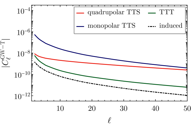
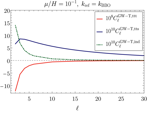
The magnitudes of the different contributions to the cross-correlation are plotted in Fig. 7. In the next section, we will consider the signatures studied in this section for a specific realisation of inflation. The analysis of the projected constraints on FNLtttsubscriptsuperscript𝐹tttNLF^{\text{ttt}}_{\rm NL} is presented in Sec. 4.6.

Refer to caption
Figure 7: The cross-correlation of the SGWB anisotropies as a function of \ell plotted for |F~NLtts|=|FNLttt|=103subscriptsuperscript~𝐹ttsNLsubscriptsuperscript𝐹tttNLsuperscript103|\tilde{F}^{\text{tts}}_{\rm NL}|=|F^{\text{ttt}}_{\rm NL}|=10^{3} and a tensor-to-scalar ratio r=0.05𝑟0.05r=0.05.

4 Constraints on the extra spin-2 setup

4.1 Description of the model

In this section, we consider an effective field theory approach to inflation comprising an extra spin-2 field σijsubscript𝜎𝑖𝑗\sigma_{ij} non-minimally coupled to the inflaton [31]. This direct coupling allows σijsubscript𝜎𝑖𝑗\sigma_{ij} to be effectively light compared to the Hubble scale (avoiding the so-called Higuchi bound [33]) and, in turn, the bispectrum to have a significant squeezed component (as already mentioned e.g. in [31, 91]). The action describing this model is given by

S=Sπ+Sσ+Sint,𝑆subscript𝑆𝜋subscript𝑆𝜎subscript𝑆intS=S_{\pi}+S_{\sigma}+S_{\rm int}\,, (4.1)

where Sπsubscript𝑆𝜋S_{\pi} denotes the standard generalised slow-roll dynamics captured by the single-field EFT approach to inflation [92], Sσsubscript𝑆𝜎S_{\sigma} is the free action for the spin-2 field σijsubscript𝜎𝑖𝑗\sigma_{ij} and Sintsubscript𝑆intS_{\rm int} contains the quadratic and cubic mixing interactions141414From here onwards τ𝜏\tau denotes conformal time and stands for differentiation with respect to conformal time.,

𝒮intsubscript𝒮int\displaystyle\mathcal{S_{\rm int}} =𝑑τd3xa4[g2ϵHa2ijπcσij+12a1gγcσijij]absentdifferential-d𝜏superscript𝑑3𝑥superscript𝑎4delimited-[]𝑔2italic-ϵ𝐻superscript𝑎2subscript𝑖subscript𝑗subscript𝜋𝑐superscript𝜎𝑖𝑗12superscript𝑎1𝑔subscriptsuperscript𝛾𝑐subscriptsuperscript𝜎𝑖𝑗𝑖𝑗\displaystyle=\;\;\,\int d\tau\,d^{3}x\,a^{4}\Big{[}-\frac{g}{\sqrt{2\epsilon}H}a^{-2}\partial_{i}\partial_{j}\pi_{c}\sigma^{ij}+\frac{1}{2}a^{-1}g\,\gamma^{\prime}_{c}\,{}_{ij}\sigma^{ij}\Big{]}\;
+dτd3xa4[g2ϵH2MPla2(a1iπcjπcσij\displaystyle\;\;+\,\int d\tau\,d^{3}x\,a^{4}\Big{[}-\frac{g}{2\epsilon H^{2}M_{\rm Pl}}a^{-2}(a^{-1}\partial_{i}\pi_{c}\partial_{j}\pi_{c}{\sigma^{\prime}}^{ij} (4.2)
+2Hiπcjπcσij)μ(σij)3+].\displaystyle\qquad\qquad\qquad\qquad\qquad+2H\partial_{i}\pi_{c}\partial_{j}\pi_{c}{\sigma}^{ij})-\mu(\sigma_{ij})^{3}+\dots\Big{]}\;.

Canonically normalising the fields, we have γcγMPlsubscript𝛾𝑐𝛾subscript𝑀Pl\gamma_{c}\equiv\gamma M_{\rm Pl}, where γijsubscript𝛾𝑖𝑗\gamma_{ij} describes the standard traceless and transverse tensor fluctuations and πc2ϵHMPlπsubscript𝜋𝑐2italic-ϵ𝐻subscript𝑀Pl𝜋\pi_{c}\equiv\sqrt{2\epsilon}HM_{\rm Pl}\,\pi. The field π𝜋\pi is the canonically normalised Goldstone boson, linearly related to the curvature fluctuation via ζHπsimilar-to-or-equals𝜁𝐻𝜋\zeta\simeq-H\pi [92]. The quantities g,μ𝑔𝜇g,\mu are coupling constants. The dots in Eq. (4.1) stand for higher-order mixing interactions.

We can decompose the spin-2 field σijsuperscript𝜎𝑖𝑗\sigma^{ij} into the helicity states as

σij=σij(0)+σij(1)+σij(2).subscript𝜎𝑖𝑗superscriptsubscript𝜎𝑖𝑗0superscriptsubscript𝜎𝑖𝑗1superscriptsubscript𝜎𝑖𝑗2\displaystyle{\sigma}_{ij}={\sigma}_{ij}^{(0)}+{\sigma}_{ij}^{(1)}+{\sigma}_{ij}^{(2)}\,. (4.3)

As usual, we may neglect helicity-1 modes as they end up being diluted by the inflationary expansion (see e.g. [93]). The (traceless and transverse) tensor degrees of freedom in the theory, γijsubscript𝛾𝑖𝑗\gamma_{ij} and σij(2)subscriptsuperscript𝜎2𝑖𝑗\sigma^{(2)}_{ij}, can be expanded in the R/L-handed basis

γij=d3k(2π)3ei𝐤𝐱λ=R/Lϵijλ(k^)γ𝐤λ(τ),subscript𝛾𝑖𝑗superscript𝑑3𝑘superscript2𝜋3superscript𝑒𝑖𝐤𝐱subscript𝜆𝑅𝐿subscriptsuperscriptitalic-ϵ𝜆𝑖𝑗^𝑘subscriptsuperscript𝛾𝜆𝐤𝜏\displaystyle\gamma_{ij}=\int\frac{d^{3}k}{(2\pi)^{3}}e^{i\mathbf{k}\cdot\mathbf{x}}\sum_{\lambda=R/L}\epsilon^{\lambda}_{ij}(\hat{k})\,\gamma^{\lambda}_{\mathbf{k}}(\tau)\,, (4.4)

and

σij(2)=d3k(2π)3ei𝐤𝐱λ=R/Lϵijλ(k^)σ𝐤2,λ(τ),subscriptsuperscript𝜎2𝑖𝑗superscript𝑑3𝑘superscript2𝜋3superscript𝑒𝑖𝐤𝐱subscript𝜆𝑅𝐿subscriptsuperscriptitalic-ϵ𝜆𝑖𝑗^𝑘subscriptsuperscript𝜎2𝜆𝐤𝜏\displaystyle\sigma^{(2)}_{ij}=\int\frac{d^{3}k}{(2\pi)^{3}}e^{i\mathbf{k}\cdot\mathbf{x}}\sum_{\lambda=R/L}\epsilon^{\lambda}_{ij}(\hat{k})\,\sigma^{2,\lambda}_{\mathbf{k}}(\tau)\,, (4.5)

where we have introduced the basis

ϵijR/Lsuperscriptsubscriptitalic-ϵ𝑖𝑗𝑅𝐿\displaystyle\epsilon_{ij}^{R/L} =12(ϵij+±iϵij×),absent12plus-or-minussuperscriptsubscriptitalic-ϵ𝑖𝑗𝑖superscriptsubscriptitalic-ϵ𝑖𝑗\displaystyle=\frac{1}{2}\left(\epsilon_{ij}^{+}\pm i\epsilon_{ij}^{\times}\right)\,, (4.6)

see App. A for more details. The polarisation tensors obey the following normalisation conventions

ϵijR/L(k^)ϵijL/R(k^)=1,subscriptsuperscriptitalic-ϵ𝑅𝐿𝑖𝑗^𝑘subscriptsuperscriptitalic-ϵ𝐿𝑅𝑖𝑗^𝑘1\displaystyle\epsilon^{R/L}_{ij}(\hat{k})\cdot\epsilon^{L/R}_{ij}(\hat{k})=1\,, (4.7)
ϵijR/L(k^)ϵijR/L(k^)=0,subscriptsuperscriptitalic-ϵ𝑅𝐿𝑖𝑗^𝑘subscriptsuperscriptitalic-ϵ𝑅𝐿𝑖𝑗^𝑘0\displaystyle\epsilon^{R/L}_{ij}(\hat{k})\cdot\epsilon^{R/L}_{ij}(\hat{k})=0\,, (4.8)
ϵijR/L(k^)=ϵijL/R(k^)=ϵijR/L(k^).subscriptsuperscriptitalic-ϵ𝑅𝐿𝑖𝑗^𝑘subscriptsuperscriptitalic-ϵ𝐿𝑅𝑖𝑗^𝑘subscriptsuperscriptitalic-ϵ𝑅𝐿𝑖𝑗^𝑘\displaystyle\epsilon^{R/L*}_{ij}(\hat{k})=\epsilon^{L/R}_{ij}(\hat{k})=\epsilon^{R/L}_{ij}(-\hat{k})\,. (4.9)

We may also write ζ𝜁\zeta and σij(0)subscriptsuperscript𝜎0𝑖𝑗\sigma^{(0)}_{ij}, as

ζ=𝜁absent\displaystyle\zeta= d3k(2π)3ei𝐤𝐱ζ𝐤(τ),superscript𝑑3𝑘superscript2𝜋3superscript𝑒𝑖𝐤𝐱subscript𝜁𝐤𝜏\displaystyle\int\frac{d^{3}k}{(2\pi)^{3}}e^{i\mathbf{k}\cdot\mathbf{x}}\zeta_{\mathbf{k}}(\tau)\,, (4.10)
σij(0)=subscriptsuperscript𝜎0𝑖𝑗absent\displaystyle\sigma^{(0)}_{ij}= d3k(2π)3ei𝐤𝐱ϵij0(k^)σ𝐤0(τ),superscript𝑑3𝑘superscript2𝜋3superscript𝑒𝑖𝐤𝐱subscriptsuperscriptitalic-ϵ0𝑖𝑗^𝑘subscriptsuperscript𝜎0𝐤𝜏\displaystyle\int\frac{d^{3}k}{(2\pi)^{3}}e^{i\mathbf{k}\cdot\mathbf{x}}\epsilon^{0}_{ij}(\hat{k})\sigma^{0}_{\mathbf{k}}(\tau)\,, (4.11)

where

ϵij0(k^)=32(k^ik^jδij3),subscriptsuperscriptitalic-ϵ0𝑖𝑗^𝑘32subscript^𝑘𝑖subscript^𝑘𝑗subscript𝛿𝑖𝑗3\displaystyle\epsilon^{0}_{ij}(\hat{k})=\sqrt{\frac{3}{2}}\left(\hat{k}_{i}\hat{k}_{j}-\frac{\delta_{ij}}{3}\right)\,, (4.12)

with ϵij0subscriptsuperscriptitalic-ϵ0𝑖𝑗\epsilon^{0}_{ij} conforming to the following normalisation rule

ϵij0(k^)ϵij0(k^)=1.subscriptsuperscriptitalic-ϵ0𝑖𝑗^𝑘subscriptsuperscriptitalic-ϵ0𝑖𝑗^𝑘1\epsilon^{0}_{ij}(\hat{k})\cdot\epsilon^{0}_{ij}(\hat{k})=1\,. (4.13)

One may proceed to quantise fields X𝐤(τ)subscript𝑋𝐤𝜏X_{\mathbf{k}}(\tau) by expanding in terms of annihilation and creation operators,

X𝐤(τ)=a𝐤u𝐤X(τ)+a𝐤u𝐤X,(τ).subscript𝑋𝐤𝜏subscript𝑎𝐤subscriptsuperscript𝑢𝑋𝐤𝜏superscriptsubscript𝑎𝐤subscriptsuperscript𝑢𝑋𝐤𝜏\displaystyle X_{\mathbf{k}}(\tau)=a_{\bf k}u^{X}_{\bf k}(\tau)+a_{-\bf k}^{\dagger}u^{X,*}_{\bf-k}(\tau)\,. (4.14)

We report below the mode functions of ζ𝜁\zeta and γ𝛾\gamma,

u𝐤ζ(τ)=iH2MPlϵk3(1+ikτ)eikτ,subscriptsuperscript𝑢𝜁𝐤𝜏𝑖𝐻2subscript𝑀𝑃𝑙italic-ϵsuperscript𝑘31𝑖𝑘𝜏superscript𝑒𝑖𝑘𝜏\displaystyle u^{\zeta}_{\bf k}(\tau)=\frac{iH}{2M_{Pl}\sqrt{\epsilon k^{3}}}(1+ik\tau)e^{-ik\tau}\,, (4.15)
u𝐤γ(τ)=2iHMPl2k3(1+ikτ)eikτ,subscriptsuperscript𝑢𝛾𝐤𝜏2𝑖𝐻subscript𝑀𝑃𝑙2superscript𝑘31𝑖𝑘𝜏superscript𝑒𝑖𝑘𝜏\displaystyle u^{\gamma}_{\bf k}(\tau)=\frac{2iH}{M_{Pl}\sqrt{2k^{3}}}(1+ik\tau)e^{-ik\tau}\,, (4.16)

and those for the σijsubscript𝜎𝑖𝑗\sigma_{ij} field,

u𝐤σ(2)(τ)=π2H(τ)3/2(c2(τ)c2i)1/2ν(1)(c2(τ)kτ),subscriptsuperscript𝑢superscript𝜎2𝐤𝜏𝜋2𝐻superscript𝜏32superscriptsubscript𝑐2𝜏subscript𝑐2𝑖12superscriptsubscript𝜈1subscript𝑐2𝜏𝑘𝜏\displaystyle u^{\sigma^{(2)}}_{\bf k}(\tau)=\sqrt{\frac{\pi}{2}}H(-\tau)^{3/2}\left(\frac{c_{2}(\tau)}{c_{2i}}\right)^{1/2}\mathcal{H}_{\nu}^{(1)}(-c_{2}(\tau)k\tau)\,, (4.17)
u𝐤σ(0)(τ)=π2H(τ)3/2(c0(τ)c0i)1/2ν(1)(c0(τ)kτ).subscriptsuperscript𝑢superscript𝜎0𝐤𝜏𝜋2𝐻superscript𝜏32superscriptsubscript𝑐0𝜏subscript𝑐0𝑖12superscriptsubscript𝜈1subscript𝑐0𝜏𝑘𝜏\displaystyle u^{\sigma^{(0)}}_{\bf k}(\tau)=\sqrt{\frac{\pi}{2}}H(-\tau)^{3/2}\left(\frac{c_{0}(\tau)}{c_{0i}}\right)^{1/2}\mathcal{H}_{\nu}^{(1)}(-c_{0}(\tau)k\tau)\,. (4.18)

Here ν=9/4(mσ2/H2)𝜈94superscriptsubscript𝑚𝜎2superscript𝐻2\nu=\sqrt{9/4-(m_{\sigma}^{2}/H^{2})}, mσsubscript𝑚𝜎m_{\sigma} being the mass of the “extra” spin-2 field, ν(1)superscriptsubscript𝜈1\mathcal{H}_{\nu}^{(1)} is the Hankel function of the first kind, and c0/2subscript𝑐02c_{0/2} denote the sound speeds of the helicity-0/2 components, with c0isubscript𝑐0𝑖c_{0i} and c2isubscript𝑐2𝑖c_{2i} the initial sound speeds. We verified151515See e.g. [94] for the full derivation of the mode functions in the case of a time-varying sound speed. Our solutions for the wave-functions coincide with those obtained in [94] in terms of canonically normalised fields. that the solutions (4.17) and (4.18) reproduce the Bunch-Davies vacuum at early times, and that they reduce to those obtained in the c0,2=subscript𝑐02absentc_{0,2}= constant case when the sound speeds are time-independent [31]. By combining together the expressions for the different sound speeds, the following independent relation follows [31]

c12=14c22+34c02,superscriptsubscript𝑐1214superscriptsubscript𝑐2234superscriptsubscript𝑐02c_{1}^{2}=\frac{1}{4}c_{2}^{2}+\frac{3}{4}c_{0}^{2}\,, (4.19)

which connects the sound speeds of the different helicity modes. We shall require that the expressions above are valid under the assumption of slowly varying sound speeds. Whenever the time dependence of the sound speeds is more sharp one ought to employ different approaches to the solutions (see e.g. [95]).

4.2 Sound speed(s) scaling

In this work we will adopt scale dependent sound speeds. This can be taken simply as an ansatz but one may show that in terms of cosmological correlators this choice corresponds, to a good approximation, to employing weakly time-dependent sound speeds. Let us start by considering the following parametrisation for the helicity-j𝑗j sound speed

cj(t)=cjiesjN+cjf,subscript𝑐𝑗𝑡superscriptsubscript𝑐𝑗𝑖superscript𝑒subscript𝑠𝑗𝑁superscriptsubscript𝑐𝑗𝑓c_{j}(t)=c_{j}^{i}\,e^{-s_{j}N}+c_{j}^{f}\,, (4.20)

where N=titH(t)𝑑t𝑁superscriptsubscriptsubscript𝑡𝑖𝑡𝐻superscript𝑡differential-dsuperscript𝑡N=\int_{t_{i}}^{t}H(t^{\prime})\,dt^{\prime} is the number of e-folds between a given reference time tisubscript𝑡𝑖t_{i} and t𝑡t, with cji=cj(ti)superscriptsubscript𝑐𝑗𝑖subscript𝑐𝑗subscript𝑡𝑖c_{j}^{i}=c_{j}(t_{i}). Our choice to add an asymptotic value cjfsuperscriptsubscript𝑐𝑗𝑓c_{j}^{f} is slightly different from the one adopted in [96]: it ensures that, regardless of the duration of inflation, there is a lower limit cjfcjimuch-less-thansuperscriptsubscript𝑐𝑗𝑓superscriptsubscript𝑐𝑗𝑖c_{j}^{f}\ll c_{j}^{i} in place for the sound speeds. This is very convenient in view of perturbativity bounds on cjsubscript𝑐𝑗c_{j} as the latter impose a lower limit on cjsubscript𝑐𝑗c_{j} of the order of 103superscript10310^{-3}. Each sjsubscript𝑠𝑗s_{j} is taken to be a constant positive parameter. Their meaning is most clear in the cjfcjiesjNmuch-less-thansuperscriptsubscript𝑐𝑗𝑓superscriptsubscript𝑐𝑗𝑖superscript𝑒subscript𝑠𝑗𝑁c_{j}^{f}\ll c_{j}^{i}\,e^{-s_{j}N} regime, where they approach the slow-roll parameter s~~𝑠\tilde{s} usually defined [97] as s~j=c˙j/cjHsubscript~𝑠𝑗subscript˙𝑐𝑗subscript𝑐𝑗𝐻\tilde{s}_{j}=\dot{c}_{j}/c_{j}H. A weak time dependence for the sound-speeds is then tantamount to requiring sj1much-less-thansubscript𝑠𝑗1s_{j}\ll 1. In conformal time Eq. (4.20) reads

cj(τ)=cji(ττi)sj+cjf,subscript𝑐𝑗𝜏superscriptsubscript𝑐𝑗𝑖superscript𝜏subscript𝜏𝑖subscript𝑠𝑗superscriptsubscript𝑐𝑗𝑓c_{j}(\tau)=c_{j}^{i}\left(\frac{\tau}{\tau_{i}}\right)^{s_{j}}+c_{j}^{f}\,, (4.21)

where for reference we take τi=1/k0subscript𝜏𝑖1subscript𝑘0\tau_{i}=1/k_{0} with k0=a0H0subscript𝑘0subscript𝑎0subscript𝐻0k_{0}=a_{0}H_{0}. It is well known that, when employing the in-in formalism for cosmological correlators, the main contribution comes from the time when mode-functions are at horizon crossing. This is because mode functions exhibit highly oscillating behaviour deep inside the(ir) horizon.
As explicit in our calculations, each σ𝜎\sigma mode function is proportional to functions of the ν(1,2)[cj(τ)kτ]superscriptsubscript𝜈12delimited-[]subscript𝑐𝑗𝜏𝑘𝜏\mathcal{H}_{\nu}^{(1,2)}[-c_{j}(\tau)\,k\tau] type, so the horizon is at cj(τ)kτ1similar-tosubscript𝑐𝑗𝜏𝑘𝜏1-c_{j}(\tau)\,k\tau\sim 1. Given that cjsubscript𝑐𝑗c_{j} values have a rather narrow range between c2isuperscriptsubscript𝑐2𝑖c_{2}^{i} and c2fsuperscriptsubscript𝑐2𝑓c_{2}^{f}, one may solve for τ𝜏\tau and verify that (i) at CMB scales (i.e. k=kCMB𝑘subscript𝑘CMBk=k_{\rm CMB}) one finds cj(τCMB)c2isimilar-to-or-equalssubscript𝑐𝑗superscript𝜏CMBsuperscriptsubscript𝑐2𝑖c_{j}(\tau^{\rm CMB})\simeq c_{2}^{i} and (ii) at e.g. BBO scales (i.e. k=kBBO𝑘subscript𝑘BBOk=k_{\rm BBO}) one finds cj(τBBO)c2fsimilar-to-or-equalssubscript𝑐𝑗superscript𝜏BBOsuperscriptsubscript𝑐2𝑓c_{j}(\tau^{\rm BBO})\simeq c_{2}^{f} to a very good approximation. This is precisely what one finds also in employing scale-dependent sound speeds:

cj(k)=cji(kk0)sj+cjf,subscript𝑐𝑗𝑘superscriptsubscript𝑐𝑗𝑖superscript𝑘subscript𝑘0subscript𝑠𝑗superscriptsubscript𝑐𝑗𝑓c_{j}(k)=c_{j}^{i}\left(\frac{k}{k_{0}}\right)^{-s_{j}}+c_{j}^{f}\,, (4.22)

which we shall adopt henceforth. The above line of reasoning is based on the notion that the key contributions to correlators come from the horizon of the mode functions at hand. This is easily verified to be the case when all wavefunctions in the integral corresponding to a given vertex share the same horizon. Whenever there are instead mode functions with different arguments (and therefore different horizons) in the same integral, the horizon of choice is clear: that corresponding to the mode that exits the horizon last (see e.g. [98, 99]). The reasoning is always the same: the integrand at any earlier time would display a highly oscillating behaviour due to at least one mode function. We will implement this criterion in all our in-in calculations.

4.3 The γγγdelimited-⟨⟩𝛾𝛾𝛾\langle\gamma\gamma\gamma\rangle and γγζdelimited-⟨⟩𝛾𝛾𝜁\langle\gamma\gamma\zeta\rangle bispectra

The mixing action in Eq. (4.1) can be made more explicit by writing it in terms of helicity-fields

𝒮intsubscript𝒮int\displaystyle\mathcal{S_{\rm int}} =𝑑τd3xa4[g2ϵHa2ijπcσ(0),ij+12a1gγcσ(2),ijij]absentdifferential-d𝜏superscript𝑑3𝑥superscript𝑎4delimited-[]𝑔2italic-ϵ𝐻superscript𝑎2subscript𝑖subscript𝑗subscript𝜋𝑐superscript𝜎0𝑖𝑗12superscript𝑎1𝑔subscriptsuperscript𝛾𝑐subscriptsuperscript𝜎2𝑖𝑗𝑖𝑗\displaystyle=\;\;\,\int d\tau\,d^{3}x\,a^{4}\Big{[}-\frac{g}{\sqrt{2\epsilon}H}a^{-2}\partial_{i}\partial_{j}\pi_{c}\sigma^{(0),ij}+\frac{1}{2}a^{-1}g\,\gamma^{\prime}_{c}\,{}_{ij}\sigma^{(2),ij}\Big{]}\;
+dτd3xa4[g2ϵH2MPla2(a1iπcjπcσ(0),ij+a1iπcjπcσ(2),ij\displaystyle\;\;+\,\int d\tau\,d^{3}x\,a^{4}\Big{[}-\frac{g}{2\epsilon H^{2}M_{\rm Pl}}a^{-2}(a^{-1}\partial_{i}\pi_{c}\partial_{j}\pi_{c}{\sigma^{\prime}}^{(0),ij}+a^{-1}\partial_{i}\pi_{c}\partial_{j}\pi_{c}{\sigma^{\prime}}^{(2),ij} (4.23)
+2Hiπcjπcσ(0),ij+2Hiπcjπcσ(2),ij)μ(σ(2),ij)33μσij(2)σjk(2)σki(2)+].\displaystyle\qquad\qquad\qquad+2H\partial_{i}\pi_{c}\partial_{j}\pi_{c}{\sigma}^{(0),ij}+2H\partial_{i}\pi_{c}\partial_{j}\pi_{c}{\sigma}^{(2),ij})-\mu(\sigma^{(2),ij})^{3}-3\mu\,\sigma^{(2)}_{ij}\cdot\sigma_{jk}^{(2)}\cdot\sigma_{ki}^{(2)}+\dots\Big{]}\;.

The interaction vertices of interest for our analysis are the following

Hσ(2)γ=d3xg2MPla3γijσ(2),ij=d3q(2π)3g2MPla3λ=R/Lγ𝐪λσ𝐪(2),λ,subscript𝐻superscript𝜎2𝛾superscript𝑑3𝑥𝑔2subscript𝑀𝑃𝑙superscript𝑎3subscriptsuperscript𝛾𝑖𝑗superscript𝜎2𝑖𝑗superscript𝑑3𝑞superscript2𝜋3𝑔2subscript𝑀𝑃𝑙superscript𝑎3subscript𝜆𝑅𝐿subscriptsuperscript𝛾𝜆𝐪subscriptsuperscript𝜎2𝜆𝐪\displaystyle H_{\sigma^{(2)}\gamma}=-\int d^{3}x\,\frac{g}{2}M_{Pl}\,a^{3}\gamma^{\prime}_{ij}\sigma^{(2),ij}=-\int\frac{d^{3}q}{(2\pi)^{3}}\,\frac{g}{2}M_{Pl}\,a^{3}\sum_{\lambda=R/L}\gamma^{\prime\lambda}_{\mathbf{q}}\,\sigma^{(2),\lambda}_{-\mathbf{q}}\,, (4.24)
H(σ(2))3=d3xμa4σij(2)σjk(2)σki(2)=d3q(2π)3d3q(2π)3d3q′′(2π)3(2π)3δ(3)(𝐪+𝐪+𝐪′′)subscript𝐻superscriptsuperscript𝜎23superscript𝑑3𝑥𝜇superscript𝑎4subscriptsuperscript𝜎2𝑖𝑗superscriptsubscript𝜎𝑗𝑘2superscriptsubscript𝜎𝑘𝑖2superscript𝑑3𝑞superscript2𝜋3superscript𝑑3superscript𝑞superscript2𝜋3superscript𝑑3superscript𝑞′′superscript2𝜋3superscript2𝜋3superscript𝛿3𝐪superscript𝐪superscript𝐪′′\displaystyle H_{(\sigma^{(2)})^{3}}=\int d^{3}x\,\mu\,a^{4}\,\sigma^{(2)}_{ij}\cdot\sigma_{jk}^{(2)}\cdot\sigma_{ki}^{(2)}=\int\frac{d^{3}q}{(2\pi)^{3}}\int\frac{d^{3}q^{\prime}}{(2\pi)^{3}}\int\frac{d^{3}q^{\prime\prime}}{(2\pi)^{3}}(2\pi)^{3}\delta^{(3)}(\mathbf{q}+\mathbf{q}^{\prime}+\mathbf{q}^{\prime\prime})
×μa4λ,λ,λ′′=R/L(ϵijλ(q^)ϵjkλ(q^)ϵkiλ′′(q^′′))σ𝐪(2),λσ𝐪(2),λσ𝐪′′(2),λ′′,absent𝜇superscript𝑎4subscript𝜆superscript𝜆superscript𝜆′′𝑅𝐿subscriptsuperscriptitalic-ϵ𝜆𝑖𝑗^𝑞superscriptsubscriptitalic-ϵ𝑗𝑘superscript𝜆superscript^𝑞superscriptsubscriptitalic-ϵ𝑘𝑖superscript𝜆′′superscript^𝑞′′subscriptsuperscript𝜎2𝜆𝐪subscriptsuperscript𝜎2superscript𝜆superscript𝐪subscriptsuperscript𝜎2superscript𝜆′′superscript𝐪′′\displaystyle\qquad\qquad\qquad\times\mu\,a^{4}\,\sum_{\lambda,\lambda^{\prime},\lambda^{{}^{\prime\prime}}=R/L}\left(\epsilon^{\lambda}_{ij}(\hat{q})\cdot\epsilon_{jk}^{\lambda^{\prime}}(\hat{q}^{\prime})\cdot\epsilon_{ki}^{\lambda^{\prime\prime}}(\hat{q}^{\prime\prime})\right)\,\sigma^{(2),\lambda}_{\mathbf{q}}\,\sigma^{(2),\lambda^{\prime}}_{\mathbf{q}^{\prime}}\,\sigma^{(2),\lambda^{\prime\prime}}_{\mathbf{q}^{\prime\prime}}\,, (4.25)
H(σ(2))2σ(0)=d3x 3μa4σij(2)σjk(2)σki(0)=d3q(2π)3d3q(2π)3d3q′′(2π)3(2π)3δ(3)(𝐪+𝐪+𝐪′′)subscript𝐻superscriptsuperscript𝜎22superscript𝜎0superscript𝑑3𝑥3𝜇superscript𝑎4subscriptsuperscript𝜎2𝑖𝑗superscriptsubscript𝜎𝑗𝑘2superscriptsubscript𝜎𝑘𝑖0superscript𝑑3𝑞superscript2𝜋3superscript𝑑3superscript𝑞superscript2𝜋3superscript𝑑3superscript𝑞′′superscript2𝜋3superscript2𝜋3superscript𝛿3𝐪superscript𝐪superscript𝐪′′\displaystyle H_{(\sigma^{(2)})^{2}\sigma^{(0)}}=\int d^{3}x\,3\mu\,a^{4}\,\sigma^{(2)}_{ij}\cdot\sigma_{jk}^{(2)}\cdot\sigma_{ki}^{(0)}=\int\frac{d^{3}q}{(2\pi)^{3}}\int\frac{d^{3}q^{\prime}}{(2\pi)^{3}}\int\frac{d^{3}q^{\prime\prime}}{(2\pi)^{3}}(2\pi)^{3}\delta^{(3)}(\mathbf{q}+\mathbf{q}^{\prime}+\mathbf{q}^{\prime\prime})
×332μa4λ,λ=R/L(q^iq^lϵijλ(q^)ϵjlλ(q^′′)13ϵijλ(q^)ϵijλ(q^′′))σ𝐪(0)σ𝐪(2),λσ𝐪′′(2),λ,absent332𝜇superscript𝑎4subscript𝜆superscript𝜆𝑅𝐿subscript^𝑞𝑖subscript^𝑞𝑙subscriptsuperscriptitalic-ϵ𝜆𝑖𝑗superscript^𝑞superscriptsubscriptitalic-ϵ𝑗𝑙superscript𝜆superscript^𝑞′′13subscriptsuperscriptitalic-ϵ𝜆𝑖𝑗superscript^𝑞superscriptsubscriptitalic-ϵ𝑖𝑗superscript𝜆superscript^𝑞′′subscriptsuperscript𝜎0𝐪subscriptsuperscript𝜎2𝜆superscript𝐪subscriptsuperscript𝜎2superscript𝜆superscript𝐪′′\displaystyle\qquad\qquad\qquad\times 3\sqrt{\frac{3}{2}}\mu\,a^{4}\,\sum_{\lambda,\lambda^{\prime}=R/L}\left(\hat{q}_{i}\hat{q}_{l}\cdot\epsilon^{\lambda}_{ij}(\hat{q}^{\prime})\cdot\epsilon_{jl}^{\lambda^{\prime}}(\hat{q}^{\prime\prime})-\frac{1}{3}\epsilon^{\lambda}_{ij}(\hat{q}^{\prime})\cdot\epsilon_{ij}^{\lambda^{\prime}}(\hat{q}^{\prime\prime})\right)\,\sigma^{(0)}_{\mathbf{q}}\,\sigma^{(2),\lambda}_{\mathbf{q}^{\prime}}\,\sigma^{(2),\lambda^{\prime}}_{\mathbf{q}^{\prime\prime}}\,, (4.26)
Hσ(0)ζ=d3xgHMPla2ijζσ(0),ij=d3q(2π)323gHMPla2q2ζ𝐪σ𝐪(0).subscript𝐻superscript𝜎0𝜁superscript𝑑3𝑥𝑔𝐻subscript𝑀𝑃𝑙superscript𝑎2subscript𝑖subscript𝑗𝜁superscript𝜎0𝑖𝑗superscript𝑑3𝑞superscript2𝜋323𝑔𝐻subscript𝑀𝑃𝑙superscript𝑎2superscript𝑞2subscript𝜁𝐪subscriptsuperscript𝜎0𝐪\displaystyle H_{\sigma^{(0)}\zeta}=-\int d^{3}x\,\frac{g}{H}M_{Pl}\,a^{2}\partial_{i}\partial_{j}\zeta\,\sigma^{(0),ij}=\int\frac{d^{3}q}{(2\pi)^{3}}\,\sqrt{\frac{2}{3}}\,\frac{g}{H}M_{Pl}\,a^{2}q^{2}\,\zeta_{\mathbf{q}}\,\sigma^{(0)}_{-\mathbf{q}}\,. (4.27)

These lead to σ𝜎\sigma-mediated contributions to primordial correlators (Fig. 8), which can be evaluated with in-in techniques. In this work we are interested in the effects of such contributions to the three point functions γγζdelimited-⟨⟩𝛾𝛾𝜁\langle\gamma\gamma\zeta\rangle and γγγdelimited-⟨⟩𝛾𝛾𝛾\langle\gamma\gamma\gamma\rangle. In particular, we are interested in those diagrams that end up giving the leading contributions to the three-point correlators above in view of our sampling the c21much-less-thansubscript𝑐21c_{2}\ll 1 region of parameter space. As we show in Secs. 2 and 3, this regime is the one for which the effect of primordial correlators on GW anisotropies is the strongest.
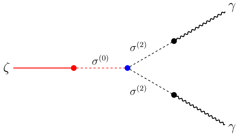
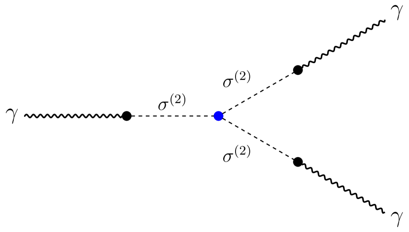
Refer to caption
Refer to caption
Figure 8: Leading σ𝜎\sigma-mediated contributions to γγζdelimited-⟨⟩𝛾𝛾𝜁\langle\gamma\gamma\zeta\rangle and γγγdelimited-⟨⟩𝛾𝛾𝛾\langle\gamma\gamma\gamma\rangle. Straight lines correspond to ζ𝜁\zeta, wiggly lines correspond to γ𝛾\gamma, red (black) dashed lines correspond to σ(0)superscript𝜎0\sigma^{(0)} (σ(2)superscript𝜎2\sigma^{(2)}) fields.

It is worth at this stage to comment on the squeezed limit of the STT and TTT correlators and consistency relations. For single-field slow-roll models inflation it is known [98, 100] that the leading contribution of these bispectra in the squeezed limit is in fact a gauge artifact. The physical contribution is instead to be found at sub-leading order (i.e. one typically pays the price of a kL2/kS2superscriptsubscript𝑘𝐿2superscriptsubscript𝑘𝑆2k_{L}^{2}/k_{S}^{2} suppression). Consistency relations may instead be broken161616We write “broken” to conform to standard terminology here. For our purposes it is enough for consistency relation to be modified, they can still be in place. In single field slow-roll the leading contribution to the three-point function has the same effect as a gauge transformation. In multi-field models it is often the case that a specific linear combination of different contributions to a diagram may be described as a gauge transformation, but, crucially, not each contribution taken on its own. There may be, in the multi-field case, more than one field that non-linearly transforms under the diffeomorphism behind the consistency relation and that is why it is a linear combination of contributions to correspond to the gauge transformation. See e.g. [101] for interesting examples along these lines. in multi-field scenarios, for non-Bunch-Davies initial conditions, in the case of non-attractor (followed by an attractor phase) solutions and for models with non-standard symmetry breaking patterns (e.g. solid inflation), to name a few. For the model at hand, it is straightforward to show the breaking of consistency conditions parametrically, in that certain coefficients appear only at cubic order and are not present in the (tree-level) power spectra [31, 91]. The diagrams under study then give a contribution that is both the leading one and physical. The main σ𝜎\sigma-mediated diagram in the γγγdelimited-⟨⟩𝛾𝛾𝛾\langle\gamma\gamma\gamma\rangle bispectrum is given by

γk1λ1γk2λ2γk3λ3=(2π)3δ(3)(k1+k2+k3)𝒜λ1λ2λ3Bttt(k1,k2,k3),delimited-⟨⟩superscriptsubscript𝛾subscript𝑘1subscript𝜆1superscriptsubscript𝛾subscript𝑘2subscript𝜆2superscriptsubscript𝛾subscript𝑘3subscript𝜆3superscript2𝜋3superscript𝛿3subscript𝑘1subscript𝑘2subscript𝑘3superscript𝒜subscript𝜆1subscript𝜆2subscript𝜆3subscript𝐵tttsubscript𝑘1subscript𝑘2subscript𝑘3\displaystyle\langle\gamma_{k_{1}}^{\lambda_{1}}\gamma_{k_{2}}^{\lambda_{2}}\gamma_{k_{3}}^{\lambda_{3}}\rangle=(2\pi)^{3}\delta^{(3)}(\vec{k}_{1}+\vec{k}_{2}+\vec{k}_{3})\,\mathcal{A}^{\lambda_{1}\lambda_{2}\lambda_{3}}B_{\rm ttt}(k_{1},k_{2},k_{3})\,, (4.28)

where the function Bttt(k1,k2,k3)subscript𝐵tttsubscript𝑘1subscript𝑘2subscript𝑘3B_{\rm ttt}(k_{1},k_{2},k_{3}) in the squeezed limit kL=k3k1k2=kSsubscript𝑘𝐿subscript𝑘3much-less-thansubscript𝑘1similar-to-or-equalssubscript𝑘2subscript𝑘𝑆k_{L}=k_{3}\ll k_{1}\simeq k_{2}=k_{S} reads

Bttt(kS,kS,kL)=24×2νπ2kS9/2νkL3/2+νμH(gMPl)3(c2(kS)c2i)5/2(c2(kL)c2i)1/2(c2,ν),subscript𝐵tttsubscript𝑘𝑆subscript𝑘𝑆subscript𝑘𝐿24superscript2𝜈superscript𝜋2superscriptsubscript𝑘𝑆92𝜈superscriptsubscript𝑘𝐿32𝜈𝜇𝐻superscript𝑔subscript𝑀Pl3superscriptsubscript𝑐2subscript𝑘𝑆subscript𝑐2𝑖52superscriptsubscript𝑐2subscript𝑘𝐿subscript𝑐2𝑖12subscript𝑐2𝜈\displaystyle B_{\rm ttt}(k_{S},k_{S},k_{L})=\frac{24\times 2^{\nu}\pi^{2}}{k_{S}^{9/2-\nu}k_{L}^{3/2+\nu}}\frac{\mu}{H}\left(\frac{g}{M_{\rm Pl}}\right)^{3}\left(\frac{c_{2}(k_{S})}{c_{2i}}\right)^{5/2}\left(\frac{c_{2}(k_{L})}{c_{2i}}\right)^{1/2}\mathcal{I}(c_{2},\nu)\,, (4.29)

and

𝒜λ1λ2λ3superscript𝒜subscript𝜆1subscript𝜆2subscript𝜆3\displaystyle\mathcal{A}^{\lambda_{1}\lambda_{2}\lambda_{3}} =ϵijλ1(k^1)ϵjlλ2(k^2)ϵlkλ1(k^3).absentsubscriptsuperscriptitalic-ϵsubscript𝜆1𝑖𝑗subscript^𝑘1subscriptsuperscriptitalic-ϵsubscript𝜆2𝑗𝑙subscript^𝑘2subscriptsuperscriptitalic-ϵsubscript𝜆1𝑙𝑘subscript^𝑘3\displaystyle=\epsilon^{\lambda_{1}}_{ij}(\hat{k}_{1})\epsilon^{\lambda_{2}}_{jl}(\hat{k}_{2})\epsilon^{\lambda_{1}}_{lk}(\hat{k}_{3})\,. (4.30)

In the same limit the quantity 𝒜𝒜\mathcal{A} reads

𝒜λ1λ2λ3|sq.=12k^Sik^Sjϵijλ1(k^L)×{1ifλ1=λ20ifλ1λ2.evaluated-atsuperscript𝒜subscript𝜆1subscript𝜆2subscript𝜆3sq12superscriptsubscript^𝑘𝑆𝑖superscriptsubscript^𝑘𝑆𝑗superscriptsubscriptitalic-ϵ𝑖𝑗subscript𝜆1subscript^𝑘𝐿cases1ifsubscript𝜆1subscript𝜆2otherwise0ifsubscript𝜆1subscript𝜆2otherwise\displaystyle\mathcal{A}^{\lambda_{1}\lambda_{2}\lambda_{3}}|_{\rm sq.}=-\frac{1}{2}\hat{k}_{S}^{i}\hat{k}_{S}^{j}\,\epsilon_{ij}^{\lambda_{1}}(\hat{k}_{L})\times\begin{cases}1\quad\mbox{if}\qquad\lambda_{1}=\lambda_{2}\\ 0\quad\mbox{if}\qquad\lambda_{1}\neq\lambda_{2}\end{cases}\,. (4.31)

The function (c2,ν)subscript𝑐2𝜈\mathcal{I}(c_{2},\nu) is given by Eq. (B.35) upon replacing c0subscript𝑐0c_{0} with c2subscript𝑐2c_{2}, obtaining

(c2,ν)subscript𝑐2𝜈\displaystyle\mathcal{I}(c_{2},\nu) =\displaystyle= Γ(ν)c2ν(kS)0𝑑x1x1𝑑x2x2𝑑x3(x1)1/2Γ𝜈subscriptsuperscript𝑐𝜈2subscript𝑘𝑆superscriptsubscript0differential-dsubscript𝑥1superscriptsubscriptsubscript𝑥1differential-dsubscript𝑥2superscriptsubscriptsubscript𝑥2differential-dsubscript𝑥3superscriptsubscript𝑥112\displaystyle\frac{\Gamma(\nu)}{c^{\nu}_{2}(k_{S})}\int_{-\infty}^{0}dx_{1}\int_{-\infty}^{x_{1}}dx_{2}\int_{-\infty}^{x_{2}}dx_{3}\,(-x_{1})^{-1/2}\, (4.32)
×{(x2)1/2ν(x3)1/2×sin[x1]Im[eix3ν(1)(c2(kS)x2)ν(2)(c2(kS)x3)]\displaystyle\times\Big{\{}(-x_{2})^{1/2-\nu}(-x_{3})^{-1/2}\,\times\sin[-x_{1}]\text{Im}\left[e^{ix_{3}}\mathcal{H}_{\nu}^{(1)}(-c_{2}(k_{S})x_{2})\mathcal{H}_{\nu}^{(2)}(-c_{2}(k_{S})x_{3})\right]
×Im[ν(1)(c2(kS)x1)ν(2)(c2(kS)x2)]+absentlimit-fromImdelimited-[]superscriptsubscript𝜈1subscript𝑐2subscript𝑘𝑆subscript𝑥1superscriptsubscript𝜈2subscript𝑐2subscript𝑘𝑆subscript𝑥2\displaystyle\quad\quad\times\text{Im}\left[\mathcal{H}_{\nu}^{(1)}(-c_{2}(k_{S})x_{1})\mathcal{H}_{\nu}^{(2)}(-c_{2}(k_{S})x_{2})\right]+
+(x2)1/2(x3)1/2νsin[x1]sin[x2]Im[ν(1)(c2(kS)x3)ν(1)(c2(kS)x3)\displaystyle\quad+(-x_{2})^{-1/2}(-x_{3})^{1/2-\nu}\sin[-x_{1}]\sin[-x_{2}]\,\text{Im}\Big{[}\mathcal{H}_{\nu}^{(1)}(-c_{2}(k_{S})x_{3})\mathcal{H}_{\nu}^{(1)}(-c_{2}(k_{S})x_{3})
×ν(2)(c2(kS)x1)ν(2)(c2(kS)x2)]}×\displaystyle\quad\quad\quad\times\mathcal{H}_{\nu}^{(2)}(-c_{2}(k_{S})x_{1})\mathcal{H}_{\nu}^{(2)}(-c_{2}(k_{S})x_{2})\Big{]}\Big{\}}\times
×(0𝑑y(y)1/2Re[eiyν(1)(c2(kL)y)]),absentsuperscriptsubscript0differential-d𝑦superscript𝑦12Redelimited-[]superscript𝑒𝑖𝑦superscriptsubscript𝜈1subscript𝑐2subscript𝑘𝐿𝑦\displaystyle\times\left(\int_{-\infty}^{0}dy\,(-y)^{-1/2}\text{Re}\left[e^{-iy}\mathcal{H}_{\nu}^{(1)}(-c_{2}(k_{L})y)\right]\right)\,,

and is well-fit by the following power law in c2subscript𝑐2c_{2}

(c2,ν)a(ν)c2(kL)νc2(kS)3ν,similar-to-or-equalssubscript𝑐2𝜈𝑎𝜈subscript𝑐2superscriptsubscript𝑘𝐿𝜈subscript𝑐2superscriptsubscript𝑘𝑆3𝜈\displaystyle\mathcal{I}(c_{2},\nu)\simeq\frac{a(\nu)}{c_{2}(k_{L})^{\nu}c_{2}(k_{S})^{3\nu}}\,, (4.33)

where a𝑎a is a parameter dependent on ν𝜈\nu (see Tab. 2 for a sample set of possible values). By proceeding in a similar fashion (see App. B for technical details), we obtain the following σ𝜎\sigma-mediated contribution to γγζdelimited-⟨⟩𝛾𝛾𝜁\langle\gamma\gamma\zeta\rangle

γk1λ1γk2λ2ζk3=(2π)3δ(3)(k1+k2+k3)𝒜λ1λ2Btts(k1,k2,k3),delimited-⟨⟩superscriptsubscript𝛾subscript𝑘1subscript𝜆1superscriptsubscript𝛾subscript𝑘2subscript𝜆2subscript𝜁subscript𝑘3superscript2𝜋3superscript𝛿3subscript𝑘1subscript𝑘2subscript𝑘3superscript𝒜subscript𝜆1subscript𝜆2subscript𝐵ttssubscript𝑘1subscript𝑘2subscript𝑘3\displaystyle\langle\gamma_{k_{1}}^{\lambda_{1}}\gamma_{k_{2}}^{\lambda_{2}}\zeta_{k_{3}}\rangle=(2\pi)^{3}\delta^{(3)}(\vec{k}_{1}+\vec{k}_{2}+\vec{k}_{3})\,\mathcal{A}^{\lambda_{1}\lambda_{2}}B_{\rm tts}(k_{1},k_{2},k_{3})\,, (4.34)

where the function Btts(k1,k2,k3)subscript𝐵ttssubscript𝑘1subscript𝑘2subscript𝑘3B_{\rm tts}(k_{1},k_{2},k_{3}) in the squeezed limit kL=k3k1k2=kSsubscript𝑘𝐿subscript𝑘3much-less-thansubscript𝑘1similar-to-or-equalssubscript𝑘2subscript𝑘𝑆k_{L}=k_{3}\ll k_{1}\simeq k_{2}=k_{S} is given by

Btts(kL,kS,kS)=subscript𝐵ttssubscript𝑘𝐿subscript𝑘𝑆subscript𝑘𝑆absent\displaystyle B_{\rm tts}(k_{L},k_{S},k_{S})= 2π2ϵμH(gMPl)32νkS9/2νkL3/2+ν(c2(kS)c2i)2(c0(kS)c0i)1/2(c0(kL)c0i)1/22superscript𝜋2italic-ϵ𝜇𝐻superscript𝑔subscript𝑀𝑃𝑙3superscript2𝜈superscriptsubscript𝑘𝑆92𝜈superscriptsubscript𝑘𝐿32𝜈superscriptsubscript𝑐2subscript𝑘𝑆subscript𝑐2𝑖2superscriptsubscript𝑐0subscript𝑘𝑆subscript𝑐0𝑖12superscriptsubscript𝑐0subscript𝑘𝐿subscript𝑐0𝑖12\displaystyle-\,\frac{2\pi^{2}}{\epsilon}\frac{\mu}{H}\left(\frac{g}{M_{Pl}}\right)^{3}\,\frac{2^{\nu}}{k_{S}^{9/2-\nu}k_{L}^{3/2+\nu}}\left(\frac{c_{2}(k_{S})}{c_{2i}}\right)^{2}\left(\frac{c_{0}(k_{S})}{c_{0i}}\right)^{1/2}\left(\frac{c_{0}(k_{L})}{c_{0i}}\right)^{1/2}\,
×(c0,c2,ν),absentsubscript𝑐0subscript𝑐2𝜈\displaystyle\times\mathcal{I}(c_{0},c_{2},\nu)\,, (4.35)

and

𝒜λ1λ2superscript𝒜subscript𝜆1subscript𝜆2\displaystyle\mathcal{A}^{\lambda_{1}\lambda_{2}} =(ϵijλ1(k^1)ϵijλ2(k^2)3k^3ik^3lϵijλ1(k^1)ϵjlλ2(k^2)).absentsubscriptsuperscriptitalic-ϵsubscript𝜆1𝑖𝑗subscript^𝑘1superscriptsubscriptitalic-ϵ𝑖𝑗subscript𝜆2subscript^𝑘23superscriptsubscript^𝑘3𝑖superscriptsubscript^𝑘3𝑙subscriptsuperscriptitalic-ϵsubscript𝜆1𝑖𝑗subscript^𝑘1superscriptsubscriptitalic-ϵ𝑗𝑙subscript𝜆2subscript^𝑘2\displaystyle=\left(\epsilon^{\lambda_{1}}_{ij}(\hat{k}_{1})\cdot\epsilon_{ij}^{\lambda_{2}}(\hat{k}_{2})-3\,\hat{k}_{3}^{i}\hat{k}_{3}^{l}\cdot\epsilon^{\lambda_{1}}_{ij}(\hat{k}_{1})\cdot\epsilon_{jl}^{\lambda_{2}}(\hat{k}_{2})\right)\,. (4.36)

In the squeezed limit 𝒜𝒜\mathcal{A} simplifies to

𝒜sq.λ1λ2=4π5MY2M(k^L)Y2M(k^S)×{1ifλ1=λ20ifλ1λ2.subscriptsuperscript𝒜subscript𝜆1subscript𝜆2sq4𝜋5subscript𝑀subscript𝑌2𝑀subscript^𝑘𝐿subscriptsuperscript𝑌2𝑀subscript^𝑘𝑆cases1ifsubscript𝜆1subscript𝜆2otherwise0ifsubscript𝜆1subscript𝜆2otherwise\mathcal{A}^{\lambda_{1}\lambda_{2}}_{\rm sq.}=\frac{4\pi}{5}\sum_{M}Y_{2M}(\hat{k}_{L})\,Y^{*}_{2M}(\hat{k}_{S})\times\begin{cases}1\quad\mbox{if}\qquad\lambda_{1}=\lambda_{2}\\ 0\quad\mbox{if}\qquad\lambda_{1}\neq\lambda_{2}\end{cases}\,. (4.37)

The function (c0,c2,ν)subscript𝑐0subscript𝑐2𝜈\mathcal{I}(c_{0},c_{2},\nu) is given by Eq. (B.35), which reads

(c0,c2,ν)subscript𝑐0subscript𝑐2𝜈\displaystyle\mathcal{I}(c_{0},c_{2},\nu) =\displaystyle= Γ(ν)c0ν(kS)0𝑑x1x1𝑑x2x2𝑑x3(x1)1/2Γ𝜈subscriptsuperscript𝑐𝜈0subscript𝑘𝑆superscriptsubscript0differential-dsubscript𝑥1superscriptsubscriptsubscript𝑥1differential-dsubscript𝑥2superscriptsubscriptsubscript𝑥2differential-dsubscript𝑥3superscriptsubscript𝑥112\displaystyle\frac{\Gamma(\nu)}{c^{\nu}_{0}(k_{S})}\int_{-\infty}^{0}dx_{1}\int_{-\infty}^{x_{1}}dx_{2}\int_{-\infty}^{x_{2}}dx_{3}\,(-x_{1})^{-1/2}\, (4.38)
×{(x2)1/2ν(x3)1/2×sin[x1]Im[eix3ν(1)(c2(kS)x2)ν(2)(c2(kS)x3)]\displaystyle\times\Big{\{}(-x_{2})^{1/2-\nu}(-x_{3})^{-1/2}\,\times\sin[-x_{1}]\text{Im}\left[e^{ix_{3}}\mathcal{H}_{\nu}^{(1)}(-c_{2}(k_{S})x_{2})\mathcal{H}_{\nu}^{(2)}(-c_{2}(k_{S})x_{3})\right]
×Im[ν(1)(c2(kS)x1)ν(2)(c2(kS)x2)]+absentlimit-fromImdelimited-[]superscriptsubscript𝜈1subscript𝑐2subscript𝑘𝑆subscript𝑥1superscriptsubscript𝜈2subscript𝑐2subscript𝑘𝑆subscript𝑥2\displaystyle\quad\quad\times\text{Im}\left[\mathcal{H}_{\nu}^{(1)}(-c_{2}(k_{S})x_{1})\mathcal{H}_{\nu}^{(2)}(-c_{2}(k_{S})x_{2})\right]+
+(x2)1/2(x3)1/2νsin[x1]sin[x2]Im[ν(1)(c2(kS)x3)ν(1)(c2(kS)x3)\displaystyle\quad+(-x_{2})^{-1/2}(-x_{3})^{1/2-\nu}\sin[-x_{1}]\sin[-x_{2}]\,\text{Im}\Big{[}\mathcal{H}_{\nu}^{(1)}(-c_{2}(k_{S})x_{3})\mathcal{H}_{\nu}^{(1)}(-c_{2}(k_{S})x_{3})
×ν(2)(c2(kS)x1)ν(2)(c2(kS)x2)]}×\displaystyle\quad\quad\quad\times\mathcal{H}_{\nu}^{(2)}(-c_{2}(k_{S})x_{1})\mathcal{H}_{\nu}^{(2)}(-c_{2}(k_{S})x_{2})\Big{]}\Big{\}}\times
×(0𝑑y(y)1/2Re[eiyν(1)(c0(kL)y)]),absentsuperscriptsubscript0differential-d𝑦superscript𝑦12Redelimited-[]superscript𝑒𝑖𝑦superscriptsubscript𝜈1subscript𝑐0subscript𝑘𝐿𝑦\displaystyle\times\left(\int_{-\infty}^{0}dy\,(-y)^{-1/2}\text{Re}\left[e^{-iy}\mathcal{H}_{\nu}^{(1)}(-c_{0}(k_{L})y)\right]\right)\,,

and is well fit by the following power law in c0subscript𝑐0c_{0} and c2subscript𝑐2c_{2}, Eq. (B.37),

(c0,c2,ν)a(ν)c0(kL)νc0(kS)νc2(kS)2ν.similar-to-or-equalssubscript𝑐0subscript𝑐2𝜈𝑎𝜈subscript𝑐0superscriptsubscript𝑘𝐿𝜈subscript𝑐0superscriptsubscript𝑘𝑆𝜈subscript𝑐2superscriptsubscript𝑘𝑆2𝜈\displaystyle\mathcal{I}(c_{0},c_{2},\nu)\simeq\frac{a(\nu)}{c_{0}(k_{L})^{\nu}c_{0}(k_{S})^{\nu}c_{2}(k_{S})^{2\nu}}\,. (4.39)

The key quantities that provide a handle on non-Gaussianities via GW anisotropies are FNLttt(kS,kL)subscriptsuperscript𝐹tttNLsubscript𝑘𝑆subscript𝑘𝐿F^{\rm ttt}_{\rm NL}(\vec{k}_{S},\vec{k}_{L}) and FNLtts(kS,kL)subscriptsuperscript𝐹ttsNLsubscript𝑘𝑆subscript𝑘𝐿F^{\rm tts}_{\rm NL}(\vec{k}_{S},\vec{k}_{L}), defined respectively in Eq. (2.12) and Eq. (2.6). The full scalar and tensor power spectra of the model under scrutiny are given by (see also [31, 32])

Pζ(k)=subscript𝑃𝜁𝑘absent\displaystyle P_{\zeta}(k)= H24MPl2ϵk3[1+𝒞ζ(ν)ϵc02ν(k)(c0(k)c0i)(gH)2],superscript𝐻24subscriptsuperscript𝑀2𝑃𝑙italic-ϵsuperscript𝑘3delimited-[]1subscript𝒞𝜁𝜈italic-ϵsubscriptsuperscript𝑐2𝜈0𝑘subscript𝑐0𝑘subscript𝑐0𝑖superscript𝑔𝐻2\displaystyle\frac{H^{2}}{4M^{2}_{Pl}\epsilon k^{3}}\left[1+\frac{\mathcal{C}_{\zeta}(\nu)}{\epsilon c^{2\nu}_{0}(k)}\left(\frac{c_{0}(k)}{c_{0i}}\right)\left(\frac{g}{H}\right)^{2}\right]\,, (4.40)
Pγ(k)=subscript𝑃𝛾𝑘absent\displaystyle P_{\gamma}(k)= 4H2MPl2k3[1+𝒞γ(ν)c22ν(k)(c2(k)c2i)(gH)2],4superscript𝐻2subscriptsuperscript𝑀2𝑃𝑙superscript𝑘3delimited-[]1subscript𝒞𝛾𝜈subscriptsuperscript𝑐2𝜈2𝑘subscript𝑐2𝑘subscript𝑐2𝑖superscript𝑔𝐻2\displaystyle\frac{4H^{2}}{M^{2}_{Pl}k^{3}}\left[1+\frac{\mathcal{C}_{\gamma}(\nu)}{c^{2\nu}_{2}(k)}\left(\frac{c_{2}(k)}{c_{2i}}\right)\left(\frac{g}{H}\right)^{2}\right]\,, (4.41)

where the analytical form of the ν𝜈\nu-dependent functions 𝒞ζ(ν)subscript𝒞𝜁𝜈\mathcal{C}_{\zeta}(\nu) and 𝒞γ(ν)subscript𝒞𝛾𝜈\mathcal{C}_{\gamma}(\nu) can be found in Ref. [31] in some specific configurations. Our interest lies in GW anisotropies at intermediate and small scales. The EFT at hand can deliver sufficiently large GW spectrum and anisotropic component at the appropriate frequencies provided we work in the c21much-less-thansubscript𝑐21c_{2}\ll 1 regime. A small helicity-2 sound speed at all scales may run afoul of non-Gaussianity bounds from CMB measurements. It is therefore convenient to consider a scale dependent c2subscript𝑐2c_{2}, and a blue GW spectrum in particular.

As we shall see, choosing a c2subscript𝑐2c_{2} that decreases towards smaller scales and a c0𝒪(1)similar-tosubscript𝑐0𝒪1c_{0}\sim\mathcal{O}(1) that exhibits a very limited variation across the frequency range, makes for a very interesting phenomenology. At CMB scales scalar and tensor spectra are close to those of single-field slow-roll inflation, i.e. the sourced contribution is sub-leading. Going towards smaller scales, the scalar spectrum remains largely dominated by vacuum fluctuations whilst the GW signal is due to the sourced contribution

Pζ(kL)similar-to-or-equalssubscript𝑃𝜁subscript𝑘𝐿absent\displaystyle P_{\zeta}(k_{L})\simeq H24MPl2ϵkL3,superscript𝐻24subscriptsuperscript𝑀2𝑃𝑙italic-ϵsuperscriptsubscript𝑘𝐿3\displaystyle\frac{H^{2}}{4M^{2}_{Pl}\epsilon k_{L}^{3}}\,, (4.42)
Pγ(kL)similar-to-or-equalssubscript𝑃𝛾subscript𝑘𝐿absent\displaystyle P_{\gamma}(k_{L})\simeq 4H2MPl2kL3,4superscript𝐻2subscriptsuperscript𝑀2𝑃𝑙superscriptsubscript𝑘𝐿3\displaystyle\frac{4H^{2}}{M^{2}_{Pl}k_{L}^{3}}\,, (4.43)
Pγ(kS)similar-to-or-equalssubscript𝑃𝛾subscript𝑘𝑆absent\displaystyle P_{\gamma}(k_{S})\simeq 4H2MPl2kS3𝒞γ(ν)c22ν(kS)(c2(kS)c2i)(gH)2,4superscript𝐻2subscriptsuperscript𝑀2𝑃𝑙superscriptsubscript𝑘𝑆3subscript𝒞𝛾𝜈subscriptsuperscript𝑐2𝜈2subscript𝑘𝑆subscript𝑐2subscript𝑘𝑆subscript𝑐2𝑖superscript𝑔𝐻2\displaystyle\frac{4H^{2}}{M^{2}_{Pl}k_{S}^{3}}\frac{\mathcal{C}_{\gamma}(\nu)}{c^{2\nu}_{2}(k_{S})}\left(\frac{c_{2}(k_{S})}{c_{2i}}\right)\left(\frac{g}{H}\right)^{2}\,, (4.44)

where one should picture kLsubscript𝑘𝐿k_{L} at CMB scales and kSsubscript𝑘𝑆k_{S} corresponding to e.g. PTA or interferometer frequencies. Given such behaviour for the power spectra, we may proceed to evaluate the non-linear parameters as defined in Eqs. (2.12) and (2.25), to obtain

FNLttt(kS,kL,ν)=subscriptsuperscript𝐹tttNLsubscript𝑘𝑆subscript𝑘𝐿𝜈absent\displaystyle F^{\rm ttt}_{\rm NL}(k_{S},k_{L},\nu)= 3π2 2νa(ν)Cγ(ν)(MPlH)(c2(kS)32νc2(kL)ν12c2i2)(gH)(μH)(kLkS)3/2ν,3superscript𝜋2superscript2𝜈𝑎𝜈subscript𝐶𝛾𝜈subscript𝑀𝑃𝑙𝐻subscript𝑐2superscriptsubscript𝑘𝑆32𝜈subscript𝑐2superscriptsubscript𝑘𝐿𝜈12superscriptsubscript𝑐2𝑖2𝑔𝐻𝜇𝐻superscriptsubscript𝑘𝐿subscript𝑘𝑆32𝜈\displaystyle 3\,\pi^{2}\,2^{\nu}\frac{a(\nu)}{C_{\gamma}(\nu)}\left(\frac{M_{Pl}}{H}\right)\left(\frac{c_{2}(k_{S})^{\frac{3}{2}-\nu}}{c_{2}(k_{L})^{\nu-\frac{1}{2}}\,c_{2i}^{2}}\right)\left(\frac{g}{H}\right)\left(\frac{\mu}{H}\right)\left(\frac{k_{L}}{k_{S}}\right)^{3/2-\nu}\,, (4.45)
F~NLtts(kS,kL,ν)=subscriptsuperscript~𝐹ttsNLsubscript𝑘𝑆subscript𝑘𝐿𝜈absent\displaystyle\tilde{F}^{\rm tts}_{\rm NL}(k_{S},k_{L},\nu)= 4π2 2νa(ν)Cγ(ν)(MPlH)(c2(kS)c0(kL)ν12c0(kS)ν12c2ic0i)(gH)(μH)(kLkS)32ν.4superscript𝜋2superscript2𝜈𝑎𝜈subscript𝐶𝛾𝜈subscript𝑀𝑃𝑙𝐻subscript𝑐2subscript𝑘𝑆subscript𝑐0superscriptsubscript𝑘𝐿𝜈12subscript𝑐0superscriptsubscript𝑘𝑆𝜈12subscript𝑐2𝑖subscript𝑐0𝑖𝑔𝐻𝜇𝐻superscriptsubscript𝑘𝐿subscript𝑘𝑆32𝜈\displaystyle-4\,\pi^{2}\,2^{\nu}\frac{a(\nu)}{C_{\gamma}(\nu)}\left(\frac{M_{Pl}}{H}\right)\left(\frac{c_{2}(k_{S})}{c_{0}(k_{L})^{\nu-\frac{1}{2}}c_{0}(k_{S})^{\nu-\frac{1}{2}}\,c_{2i}\,c_{0i}}\right)\left(\frac{g}{H}\right)\left(\frac{\mu}{H}\right)\left(\frac{k_{L}}{k_{S}}\right)^{\frac{3}{2}-\nu}\,. (4.46)

As clear from the common (kL/kS)3/2νsuperscriptsubscript𝑘𝐿subscript𝑘𝑆32𝜈(k_{L}/k_{S})^{3/2-\nu} scaling, a small exponent (i.e. a light field) will provide the most striking signatures for both the auto- and cross-correlations we are after. Combining Eq. (4.45) with Eq. (4.46) to obtain

FNLttt(kS,kL,ν)=34(c0ic2i)(c0(kS)c0(kL)c2(kS)c2(kL))ν12F~NLtts(kS,kL,ν),subscriptsuperscript𝐹tttNLsubscript𝑘𝑆subscript𝑘𝐿𝜈34subscript𝑐0𝑖subscript𝑐2𝑖superscriptsubscript𝑐0subscript𝑘𝑆subscript𝑐0subscript𝑘𝐿subscript𝑐2subscript𝑘𝑆subscript𝑐2subscript𝑘𝐿𝜈12subscriptsuperscript~𝐹ttsNLsubscript𝑘𝑆subscript𝑘𝐿𝜈F^{\rm ttt}_{\rm NL}(k_{S},k_{L},\nu)=-\frac{3}{4}\left(\frac{c_{0i}}{c_{2i}}\right)\left(\frac{c_{0}(k_{S})c_{0}(k_{L})}{c_{2}(k_{S})c_{2}(k_{L})}\right)^{\nu-\frac{1}{2}}\tilde{F}^{\rm tts}_{\rm NL}(k_{S},k_{L},\nu)\,, (4.47)

shows that whenever c2c0much-less-thansubscript𝑐2subscript𝑐0c_{2}\ll c_{0}, for a sufficiently light field the TTT non-linear parameter will be enhanced with respect to the TTS one.

4.4 Parameter space

Let us now discuss the parameter space of the theory. First of all, following the previous subsection, we fix the following parametrisation for the helicity-2 sound speed c2subscript𝑐2c_{2},

c2(k)=c2i(k0k)s2+c2f.subscript𝑐2𝑘subscript𝑐2𝑖superscriptsubscript𝑘0𝑘subscript𝑠2subscript𝑐2𝑓\displaystyle c_{2}(k)=c_{2i}\left(\frac{k_{0}}{k}\right)^{s_{2}}+c_{2f}\;. (4.48)

For the helicity-0 component we take the following parametrisation

c0(k)=c0i(k0k)s0.subscript𝑐0𝑘subscript𝑐0𝑖superscriptsubscript𝑘0𝑘subscript𝑠0\displaystyle c_{0}(k)=c_{0i}\left(\frac{k_{0}}{k}\right)^{s_{0}}\,. (4.49)

Note that here we are neglecting c0fsubscript𝑐0𝑓c_{0f}. The reason is that we are interested in scenarios where the running with scale of the helicity-0 sound speed is almost absent, with c0(k)1similar-to-or-equalssubscript𝑐0𝑘1c_{0}(k)\simeq 1.

A number of constraints on the parameter space of our model are already in place. These come from: (i) consistency of the theory (i.e. gradient instabilities, perturbativity); (ii) constraints on the scalar power spectrum amplitude and spectral index (e.g. it is important to keep c0subscript𝑐0c_{0} fairly close to 1 at CMB scales so that the scalar power spectrum is dominated by the vacuum and there is no issue with the spectral index being in agreement with observations); (iii) constraints on the tensor power spectrum; (iv) constraints on scalar and tensor non-Gaussianities. Points (i)-(iii) are discussed and summarised in Secs. 3.1, 3.2 and 3.3 of [32]. Point (iv) is discussed e.g. in [96].

The existing constraints on primordial non-Gaussianity at CMB scales require c2102greater-than-or-equivalent-tosubscript𝑐2superscript102c_{2}\gtrsim 10^{-2}, while one must impose c2f103greater-than-or-equivalent-tosubscript𝑐2𝑓superscript103c_{2f}\gtrsim 10^{-3} throughout due to the perturbativity bound. Moreover, taking c0isubscript𝑐0𝑖c_{0i} close to 111 with s0s2much-less-thansubscript𝑠0subscript𝑠2s_{0}\ll s_{2} implies the following relation for the sound speeds, c0c1c2similar-to-or-equalssubscript𝑐0subscript𝑐1much-greater-thansubscript𝑐2c_{0}\simeq c_{1}\gg c_{2} 171717We are assuming conservatively that the relation in Eq. (4.19) holds for scale-dependent sound speeds as well.. The momentum dependence of the sound speeds is plotted in Fig. 9 for a set of parameters that maximises the GW amplitudes at direct detection scales.
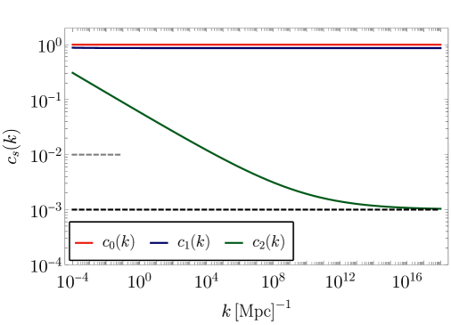
Refer to caption
Figure 9: The scale-dependence of the sound speeds cs(k)subscript𝑐𝑠𝑘c_{s}(k) taking c2i=2.5×101,c2f=103,s2=1.8×101,c0i=1,s0=0formulae-sequencesubscript𝑐2𝑖2.5superscript101formulae-sequencesubscript𝑐2𝑓superscript103formulae-sequencesubscript𝑠21.8superscript101formulae-sequencesubscript𝑐0𝑖1subscript𝑠00c_{2i}=2.5\times 10^{-1},\,c_{2f}=10^{-3},\,s_{2}=1.8\times 10^{-1},\,c_{0i}=1,\,s_{0}=0. The black and grey dashed lines show the bounds from perturbativity and CMB non-Gaussianity respectively.

Note that c0subscript𝑐0c_{0} has been chosen as large as possible (close to 1) throughout its scale dependence due to the constraint g/Hϵc02much-less-than𝑔𝐻italic-ϵsuperscriptsubscript𝑐02g/H\ll\sqrt{\epsilon c_{0}^{2}} imposed to avoid gradient instabilities [32]. This allows us to take larger values of g/H𝑔𝐻g/H, leading to an observable GW spectrum on small scales (the sourced contribution to the tensor power spectrum scales as (g/H)2superscript𝑔𝐻2(g/H)^{2}, Eq. (4.44)).
The same constraint also ensures that the sourced contribution to the scalar power spectrum is subdominant compared to the vacuum one whose amplitude and spectral index are taken to be AS=2.09×10⁹subscript𝐴𝑆2.09superscript109A_{S}=2.09\times 10^{-9} and nS=0.9649subscript𝑛𝑆0.9649n_{S}=0.9649 in accordance with the Planck values [102]. A detailed analysis of the constraints on the parameter space of this model has previously been carried out in [32, 96] and we have ensured that our choices for the parameters {cs,i,cs,f,s,μ/H,ρ/H,ν}subscript𝑐𝑠𝑖subscript𝑐𝑠𝑓𝑠𝜇𝐻𝜌𝐻𝜈\{c_{s,i},\,c_{s,f},s\,,\,\mu/H,\,\rho/H,\,\nu\} lie within the allowed region.

Refer to caption
Refer to caption
Figure 10: Left : The scalar power spectrum for the spin-2 model along with the measured power spectrum from CMB observations [102] and the constraints from various experiments (see [103, 104] for the exact constraints). Right: The different contributions to the tensor power spectrum for the spin-2 model. The choice of parameters for both panels is c2i=2.5×101,c2f=103,s2=1.8×101,c0i=1,s0=0,g/H=4×103,ν=1.45formulae-sequencesubscript𝑐2𝑖2.5superscript101formulae-sequencesubscript𝑐2𝑓superscript103formulae-sequencesubscript𝑠21.8superscript101formulae-sequencesubscript𝑐0𝑖1formulae-sequencesubscript𝑠00formulae-sequence𝑔𝐻4superscript103𝜈1.45c_{2i}=2.5\times 10^{-1},\,c_{2f}=10^{-3},\,s_{2}=1.8\times 10^{-1},\,c_{0i}=1,\,s_{0}=0,\,g/H=4\times 10^{-3},\nu=1.45.

The scalar and tensor power spectra for this model are plotted in Fig. 10 with the parameter choice c2i=2.5×101,c2f=103,s2=1.8×101,c0i=1,s0=0,g/H=4×103,ν=1.45,H/Mpl=105formulae-sequencesubscript𝑐2𝑖2.5superscript101formulae-sequencesubscript𝑐2𝑓superscript103formulae-sequencesubscript𝑠21.8superscript101formulae-sequencesubscript𝑐0𝑖1formulae-sequencesubscript𝑠00formulae-sequence𝑔𝐻4superscript103formulae-sequence𝜈1.45𝐻subscript𝑀plsuperscript105c_{2i}=2.5\times 10^{-1},\,c_{2f}=10^{-3},\,s_{2}=1.8\times 10^{-1},\,c_{0i}=1,\,s_{0}=0,\,g/H=4\times 10^{-3},\nu=1.45,\,H/M_{\rm pl}=10^{-5} and the GW spectrum is plotted in Fig. 11 for different values of c2fsubscript𝑐2𝑓c_{2f}. We see that for c2f=103subscript𝑐2𝑓superscript103c_{2f}=10^{-3}, the GW spectrum falls within the sensitivity range of SKA, Taiji and BBO as well as next generation CMB experiments like CMB-S4. For the same choice of parameters, in Fig. 12 we plot the TTS and TTT non-linearity parameters taking F~NLsubscript~𝐹NL\tilde{F}_{\rm NL} with the expressions given in Eq. (4.45) and Eq. (4.46). The expression for F~NLttssubscriptsuperscript~𝐹ttsNL\tilde{F}^{\text{tts}}_{\rm NL} is exact since the scalar power spectrum is dominated by the vacuum contribution throughout. For FNLtttsubscriptsuperscript𝐹tttNLF^{\text{ttt}}_{\rm NL}, note that since the tensor power spectrum is dominated by the sourced contribution on smaller scales Eq. (4.46) is an approximation that works well only on the largest scales (kL<102subscript𝑘𝐿superscript102k_{L}<10^{-2}). While this approximation reproduces the correct scaling as well as the order of magnitude in this range, the exact results are used for all the plots and in calculating the correlations in Sec. 4.5. The behaviour of both FNLtttsubscriptsuperscript𝐹tttNLF^{\text{ttt}}_{\rm NL} and F~NLttssubscriptsuperscript~𝐹ttsNL\tilde{F}^{\text{tts}}_{\rm NL} as a function of momentum can be understood as a result of the scale dependence arising from the factor (kL/kS)3/2νsuperscriptsubscript𝑘𝐿subscript𝑘𝑆32𝜈(k_{L}/k_{S})^{3/2-\nu}. There is also a moderate scale dependence due to the running sound speed c2subscript𝑐2c_{2} whereas c0subscript𝑐0c_{0} remains constant throughout.

Refer to caption
Figure 11: ΩGW(k)subscriptΩGW𝑘{\Omega_{{\rm{{GW}}}}}(k) for different values of c2fsubscript𝑐2𝑓c_{2f} plotted alongside the power law sensitivity curves for SKA, LISA, Taiji, BBO and ET. We also plot the current bound from the CMB as well as the expected sensitivity of CMB-S4 [105].
Refer to caption
Figure 12: The non-linearity parameters F~NL(kS,kL)subscript~𝐹NLsubscript𝑘𝑆subscript𝑘𝐿\tilde{F}_{\rm NL}(k_{S},k_{L}) for the TTS and TTT bispectra plotted as a function of kSsubscript𝑘𝑆k_{S} and kLsubscript𝑘𝐿k_{L} for μ/H=101𝜇𝐻superscript101\mu/H=10^{-1}.

4.5 Angular power spectra of GW anisotropies

With the above choice of parameters and armed with the results of Sec. 2.3 and 3, we are now able to calculate the angular power spectra of the GW anisotropies for the spin-2 model. We plot these in Fig. 13 at the frequency scales associated to BBO. We see that both the auto-correlation and the cross-correlation are dominated by the TTT contribution as a result of the small sound speed of the helicity-2 component of the spin-2 field.
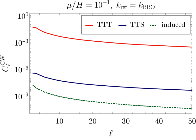
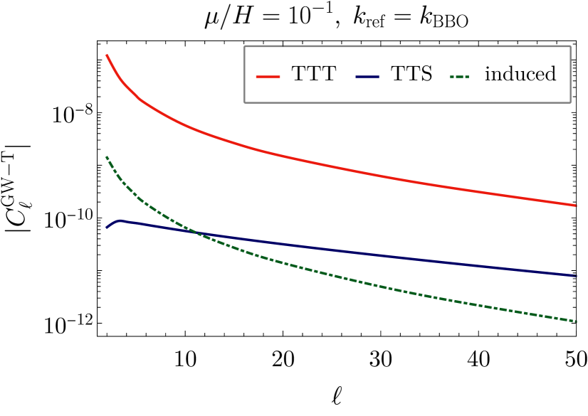
Refer to caption
Refer to caption
Figure 13: The different contributions to the auto-correlation CGWsubscriptsuperscript𝐶GWC^{\rm{GW}}_{\ell} and cross-correlation CGWTsubscriptsuperscript𝐶GWTC^{\rm{GW-T}}_{\ell} plotted for the spin-2 model. For comparison we also plot the induced anisotropies from propagation.
Refer to caption
Figure 14: The cross-correlation CGWTsubscriptsuperscript𝐶GWTC^{\rm{GW-T}}_{\ell} for the spin-2 model. For comparison we also plot the anisotropies induced by propagation.

Interestingly, as a result of the (kL/kS)3/2νsuperscriptsubscript𝑘𝐿subscript𝑘𝑆32𝜈(k_{L}/k_{S})^{3/2-\nu} scale dependence, the CMB-GW cross-correlation from the TTS bispectrum is suppressed at the largest angular scales, in particular at =22\ell=2 (Fig. 14), in contrast to the case where F~NLttssubscriptsuperscript~𝐹ttsNL\tilde{F}^{\text{tts}}_{\rm NL} is scale independent (Fig. 7). While this suppression can be a potential signature of the mass of the spin-2 field (recall that ν=9/4mσ2/H2𝜈94superscriptsubscript𝑚𝜎2superscript𝐻2\nu=\sqrt{9/4-m_{\sigma}^{2}/H^{2}}), the TTS cross-correlation is always smaller than the cross-correlation from the TTT bispectrum and thus this effect is unlikely to be observable. We also see that CGWT,ttt<0subscriptsuperscript𝐶GWTttt0C^{\rm{GW-T,ttt}}_{\ell}<0 (Fig. 14) which can be physically understood from the fact that the CMB temperature anisotropies from tensor perturbations arise from the subhorizon decay of the tensor modes. Thus, in Eq. (3.34) we have dγ/dη<0𝑑𝛾𝑑𝜂0d\gamma/d\eta<0 and so when FNLttt>0subscriptsuperscript𝐹tttNL0F^{\text{ttt}}_{\rm NL}>0 we will have CGWT,ttt<0subscriptsuperscript𝐶GWTttt0C^{\rm{GW-T,ttt}}_{\ell}<0. Additionally, the TTT and TTS cross-correlations have opposite signs which reduces the cross-correlation signal.

For reference note that the GW energy density and F~NLtts,FNLtttsubscriptsuperscript~𝐹ttsNLsubscriptsuperscript𝐹tttNL\tilde{F}^{\text{tts}}_{\rm NL},F^{\text{ttt}}_{\rm NL} at BBO scales can be approximated as a function of the model parameters μ/H,c2f𝜇𝐻subscript𝑐2𝑓\mu/H,c_{2f} as

ΩGW(kBBO)subscriptΩGWsubscript𝑘BBO\displaystyle{\Omega_{{\rm{{GW}}}}}(k_{\rm BBO}) 1.3×10¹³(c2f103)1.7,similar-to-or-equalsabsent1.3superscript1013superscriptsubscript𝑐2𝑓superscript1031.7\displaystyle\simeq 1.3\times 10^{-13}\left(\frac{c_{2f}}{10^{-3}}\right)^{-1.7},
FNLttt(kBBO,kp)subscriptsuperscript𝐹tttNLsubscript𝑘BBOsubscript𝑘𝑝\displaystyle F^{\text{ttt}}_{\rm NL}(k_{\rm BBO},k_{p}) 1.2×10⁶(μH),similar-to-or-equalsabsent1.2superscript106𝜇𝐻\displaystyle\simeq 1.2\times 10^{6}\left(\frac{\mu}{H}\right), (4.50)
F~NLtts(kBBO,kp)subscriptsuperscript~𝐹ttsNLsubscript𝑘BBOsubscript𝑘𝑝\displaystyle\tilde{F}^{\text{tts}}_{\rm NL}(k_{\rm BBO},k_{p}) 3.5×10²(μH).similar-to-or-equalsabsent3.5superscript102𝜇𝐻\displaystyle\simeq-3.5\times 10^{2}\left(\frac{\mu}{H}\right)\,.

Note that we have fixed all the other parameters to the values considered in Sec. 4.4.

As a consequence of the scale dependence of F~NLtts,FNLtttsubscriptsuperscript~𝐹ttsNLsubscriptsuperscript𝐹tttNL\tilde{F}^{\text{tts}}_{\rm NL},\,F^{\text{ttt}}_{\rm NL}, the resulting CGW,CGWTsubscriptsuperscript𝐶GWsubscriptsuperscript𝐶GWTC^{\rm{GW}}_{\ell},\,C^{\rm{GW-T}}_{\ell} will also be scale dependent181818The additional scale dependence arising from the running of the sound speed c2(k)subscript𝑐2𝑘c_{2}(k) on small scales can be safely neglected since this is nearly constant throughout (c2(kS)103similar-to-or-equalssubscript𝑐2subscript𝑘𝑆superscript103c_{2}(k_{S})\simeq 10^{-3}, see Fig. 9). , i.e.,

CGW(kref)subscriptsuperscript𝐶GWsubscript𝑘ref\displaystyle C^{\rm{GW}}_{\ell}(k_{\rm ref}) CGW(kBBO)×(kBBOkref)32ν,similar-to-or-equalsabsentsubscriptsuperscript𝐶GWsubscript𝑘BBOsuperscriptsubscript𝑘BBOsubscript𝑘ref32𝜈\displaystyle\simeq C^{\rm{GW}}_{\ell}(k_{\rm BBO})\times\left(\frac{k_{\rm BBO}}{k_{\rm ref}}\right)^{3-2\nu},
CGWT(kref)subscriptsuperscript𝐶GWTsubscript𝑘ref\displaystyle C^{\rm{GW-T}}_{\ell}(k_{\rm ref}) CGWT(kBBO)×(kBBOkref)3/2ν,similar-to-or-equalsabsentsubscriptsuperscript𝐶GWTsubscript𝑘BBOsuperscriptsubscript𝑘BBOsubscript𝑘ref32𝜈\displaystyle\simeq C^{\rm{GW-T}}_{\ell}(k_{\rm BBO})\times\left(\frac{k_{\rm BBO}}{k_{\rm ref}}\right)^{3/2-\nu}, (4.51)

for the anisotropies arising from both the TTS and TTT non-Gaussianity.

4.6 Projected constraints on FNLsubscript𝐹NLF_{\rm NL}

We can now estimate the error in the measurement of FNLsubscript𝐹NL{F}_{\rm NL}. For the spin-2 model we have seen that the anisotropies from the TTT bispectrum are dominant compared to those from the TTS bispectrum. Thus, we focus here on the error in the estimation of FNLtttsuperscriptsubscript𝐹NLttt{F}_{\rm NL}^{\rm ttt} using both auto-correlation and cross-correlation measurements (see Sec. 3.2.1 for the details).
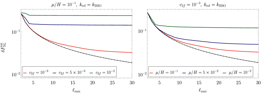
Refer to caption
Figure 15: The relative error in the measurement of FNLtttsuperscriptsubscript𝐹NLttt{F}_{\rm NL}^{\rm ttt} as a function of maxsubscriptmax\ell_{\rm max} with BBO for different values of μ,c2f𝜇subscript𝑐2𝑓\mu,c_{2f}. The dashed curves show the errors for an idealised, cosmic variance limited measurement.

In Fig. 15 we plot the relative error in the measurement of FNLtttsuperscriptsubscript𝐹NLttt{F}_{\rm NL}^{\rm ttt} defined as

δFNLtttΔFNLttt/FNLttt,𝛿superscriptsubscript𝐹NLtttΔsuperscriptsubscript𝐹NLtttsuperscriptsubscript𝐹NLttt\displaystyle\delta{F}_{\rm NL}^{\rm ttt}\equiv{\Delta{F}_{\rm NL}^{\rm ttt}}/{{F}_{\rm NL}^{\rm ttt}}\,, (4.52)

for different values of μ,c2f𝜇subscript𝑐2𝑓\mu,c_{2f}. For reference, note that at BBO scales, the GW amplitude and FNLtttsubscriptsuperscript𝐹tttNLF^{\text{ttt}}_{\rm NL} can be approximated as a function of c2f,μ/Hsubscript𝑐2𝑓𝜇𝐻c_{2f},\mu/H as given in Eq. (4.5). We see that in the case of c2f=103,μ/H=101formulae-sequencesubscript𝑐2𝑓superscript103𝜇𝐻superscript101c_{2f}=10^{-3},\mu/H=10^{-1} we can achieve a relative error δFNLttt102similar-to𝛿superscriptsubscript𝐹NLtttsuperscript102\delta{F}_{\rm NL}^{\rm ttt}\sim 10^{-2}; a similar error is achievable for the noiseless cosmic-variance limited case which is understandable from the fact that for this choice of parameters we have CGW,tttNGWmuch-greater-thansuperscriptsubscript𝐶GWtttsubscriptsuperscript𝑁GWC_{\ell}^{\rm{GW,ttt}}\gg N^{\rm{GW}}_{\ell}. For smaller values of μ𝜇\mu and larger c2fsubscript𝑐2𝑓c_{2f}, i.e. smaller FNLttt,ΩGWsuperscriptsubscript𝐹NLtttsubscriptΩGW{F}_{\rm NL}^{\rm ttt},\,{\Omega_{{\rm{{GW}}}}}, we see that the error saturates extremely quickly, around max610similar-tosubscriptmax610\ell_{\rm max}\sim 6\operatorname{--}10, due to the fact that the detector noise increases rapidly after the first few multipoles (see Fig. 3).

SNR of the CMB-GW cross-correlation

As in Sec. 3, we also estimate the signal to noise ratio of the CMB-GW cross-correlation for the spin-2 model in the presence of an astrophysical foreground.
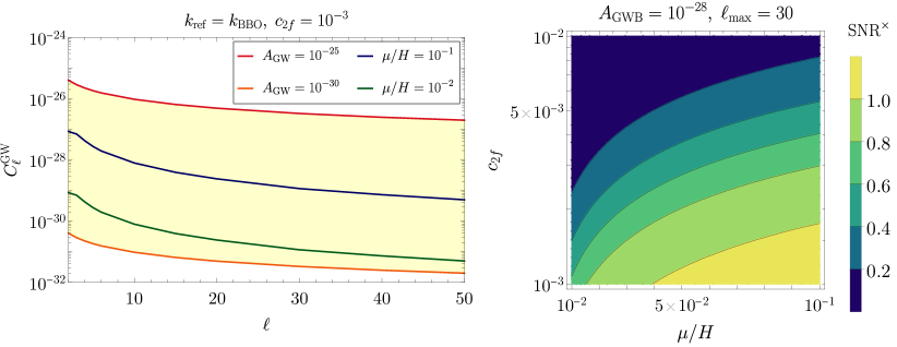
Refer to caption
Figure 16: Left: The CGWsubscriptsuperscript𝐶GWC^{\rm{GW}}_{\ell} for the astrophysical background (yellow shaded region) and for the CGWB anisotropies in the spin-2 model for different values of μ/H𝜇𝐻\mu/H taking c2f=103subscript𝑐2𝑓superscript103c_{2f}=10^{-3}. Right: Signal to noise of the total cross-correlation for the spin-2 model as a function of c2f,μ/Hsubscript𝑐2𝑓𝜇𝐻c_{2f},\,\mu/H.

To arrive at a detectable signal one needs to consider a relatively small AGWBsubscript𝐴GWBA_{\rm GWB}. This can be understood from an argument similar to the one made in Sec. 3.2. In the expression for the SNR Eq. (3.28) one has the following term,

SNR×[(2+1)(CGWT,signal)2CGW,totalCTT]1/2.similar-to-or-equalssuperscriptSNRsuperscriptdelimited-[]subscript21superscriptsuperscriptsubscriptCGWTsignal2superscriptsubscriptCGWtotalsubscriptsuperscriptCTT12\displaystyle\rm{SNR}^{\times}\simeq\left[\sum_{\ell}(2\ell+1)\frac{\left(C_{\ell}^{\rm GW-T,signal}\right)^{2}}{C_{\ell}^{\rm GW,total}C^{\rm{TT}}_{\ell}}\right]^{1/2}. (4.53)

For the spin-2 model we have seen that the CMB-GW cross-correlation as well as the auto-correlation is dominated by the TTT contribution, however the variance of the CMB temperature anisotropies is dominated by the scalar term rather than the tensor term. Thus, for the spin-2 model anisotropies, we again have CGWT,signal(CGW,totalCTT)1/2much-less-thansuperscriptsubscript𝐶GWTsignalsuperscriptsuperscriptsubscript𝐶GWtotalsubscriptsuperscript𝐶TT12C_{\ell}^{\rm GW-T,signal}\ll({C_{\ell}^{\rm GW,total}C^{\rm{TT}}_{\ell}})^{1/2} unlike that of the monopolar TTS considered in Sec. 3.2 where we found CGWT,signal(CGW,totalCTT)1/2similar-to-or-equalssuperscriptsubscript𝐶GWTsignalsuperscriptsuperscriptsubscript𝐶GWtotalsubscriptsuperscript𝐶TT12C_{\ell}^{\rm GW-T,signal}\simeq({C_{\ell}^{\rm GW,total}C^{\rm{TT}}_{\ell}})^{1/2}. Furthermore, we also see from Fig. 14 that CGWT,tttsubscriptsuperscript𝐶GWTtttC^{\rm{GW-T,ttt}}_{\ell} and CGWT,ttssubscriptsuperscript𝐶GWTttsC^{\rm{GW-T,tts}}_{\ell} for the spin-2 model have opposite signs which reduces the total signal appearing in the SNR.

5 Conclusions

During inflation, scalar and tensor quantum fluctuations are generated around the background solution. These modes eventually re-enter the horizon and “perturb” the path of any field that propagates trough structure. One such field is the massless graviton. The effect of GW propagation in a perturbed universe manifests itself in the intermediate/small scale GW power spectrum in the form of an anisotropic component (see e.g. [106, 27, 28, 29]). It is clear that such anisotropies are ultimately of inflationary origin and furthermore that they are universal in the sense that they rely on there being an inflationary phase but require no further model-dependent assumption. Naturally, detection requires the existence of an observable SGWB at the scales relevant for each given probe. In our nomenclature, these are induced anisotropies and their amplitude is typically δindGWAsζsimilar-tosubscriptsuperscript𝛿GWindsubscript𝐴𝑠similar-to𝜁\delta^{\rm GW}_{\rm ind}\sim\sqrt{A_{s}}\sim\zeta.
In this work we have studied another source of anisotropies, one that relies on the existence of sufficiently large primordial mixed and/or tensor non-Gaussianities. We have shown that, in order to be the leading source of anisotropies, this mechanism requires that the non-linear parameters satisfy: FNLtts1much-greater-thansubscriptsuperscript𝐹ttsNL1F^{\rm tts}_{\rm NL}\gg 1 and/or rFNLttt1much-greater-than𝑟subscriptsuperscript𝐹tttNL1\sqrt{r}\,F^{\rm ttt}_{\rm NL}\gg 1. These requirements limit the models that can be put to the test. On the other hand, by testing anisotropies of this nature we are automatically probing not only inflation but in particular inflationary interactions, which allows us to rule out significant regions of parameter space and possibly model space as well. Furthermore, it is often the case that the same (rich) field content that produces a GW signal within reach of e.g. PTAs or laser interferometers also has widen in the parameter space for those non-Gaussianities that give a leading contribution to GW anisotropies.
The first part of this paper took a phenomenological approach. Here we studied auto- and cross-correlations of GW anisotropies and identified the parameter space (in terms of ΩGW,FNLsubscriptΩGWsubscript𝐹NL\Omega_{\rm GW},F_{\rm NL}) that is within reach for upcoming GW probes. Our analysis revealed the importance of the angular dependence of the primordial bispectra especially in the case of cross-correlations. For pre-determined angular behaviour in the case of temperature anisotropies, having e.g. a monopolar or quadrupolar TTS signal can make the difference between having an observable cross-correlation vs an undetectable one.
The focus on a stochastic gravitational wave background of cosmological origin should not distract from the fact that there most certainly is a background of astrophysical origin. This must be negotiated within our effort to test early universe physics. We have accounted for the AGWB in our analysis, assuming its angular power spectrum amplitude varies between 1030superscript103010^{-30} and 1025superscript102510^{-25} (in the 102superscript10210^{-2} to 100similar-toabsent100\sim 100Hz range). We have seen that the use of cross-correlations with the CMB is likely the most powerful tool at our disposal in this case. Indeed, upon using cross-correlations, and depending on the parameter space, the primordial signal can be detected even when the anisotropies angular power spectrum is dominated by the AGWB component.
In the last part of this paper, we considered a concrete example of an inflationary model equipped with (i) a blue GW spectrum and (ii) sufficiently large non-Gaussian amplitude to grant a percent level relative error on FNLtttsubscriptsuperscript𝐹tttNLF^{\rm ttt}_{\rm NL} (for FNLttt104similar-tosubscriptsuperscript𝐹tttNLsuperscript104F^{\rm ttt}_{\rm NL}\sim 10^{4}105superscript10510^{5}) obtained via GW anisotropies measurements. Our specific realisation underscores the fact that, despite the unavoidable rsimilar-toabsent𝑟\sim\sqrt{r} suppression TTT-sourced anisotropies suffer w.r.t. to their TTS counterpart, it is still possible for TTT to generate the leading anisotropic component of the GW spectrum. It will be very interesting to consider other inflationary realisations for which this is not the case. Another direction worth pursuing is the study of models with a monopolar TTS contribution. We leaves these pursuits to future work.

Acknowledgements

M. F. would like to acknowledge support from the “Atracción de Talento” grant 2019-T1/TIC-15784. G.O. and P.D.M. acknowledge support from the Netherlands organisation for scientific research (NWO) VIDI grant (dossier 639.042.730).

Appendix A Helicity-2 polarisation tensors

In this section we set our conventions for the definition of the helicity-2 polarisation tensors. If the helicity-2 field wave-vector is written in polar coordinates as

k^=(sinθcosϕ,sinθsinϕ,cosθ),^𝑘𝜃italic-ϕ𝜃italic-ϕ𝜃\hat{k}=(\sin\theta\cos\phi,\sin\theta\sin\phi,\cos\theta)\,, (A.1)

we can define the linear polarisation tensors in terms of two unit vectors perpendicular to k^^𝑘\hat{k} as

ϵij+superscriptsubscriptitalic-ϵ𝑖𝑗\displaystyle\epsilon_{ij}^{+} =(u1)i(u1)j(u2)i(u2)j,absentsubscriptsubscript𝑢1𝑖subscriptsubscript𝑢1𝑗subscriptsubscript𝑢2𝑖subscriptsubscript𝑢2𝑗\displaystyle=(u_{1})_{i}(u_{1})_{j}-(u_{2})_{i}(u_{2})_{j}\,, (A.2)
ϵij×superscriptsubscriptitalic-ϵ𝑖𝑗\displaystyle\epsilon_{ij}^{\times} =(u1)i(u2)j+(u2)i(u1)j,absentsubscriptsubscript𝑢1𝑖subscriptsubscript𝑢2𝑗subscriptsubscript𝑢2𝑖subscriptsubscript𝑢1𝑗\displaystyle=(u_{1})_{i}(u_{2})_{j}+(u_{2})_{i}(u_{1})_{j}\,, (A.3)

where

u1=(sinϕ,cosϕ,0),u2={(cosθcosϕ,cosθsinϕ,sinθ)if θ<π/2(cosθcosϕ,cosθsinϕ,sinθ)if θ>π/2.formulae-sequencesubscript𝑢1italic-ϕitalic-ϕ0subscript𝑢2cases𝜃italic-ϕ𝜃italic-ϕ𝜃if 𝜃𝜋2otherwise𝜃italic-ϕ𝜃italic-ϕ𝜃if 𝜃𝜋2otherwiseu_{1}=\left(\sin\phi,-\cos\phi,0\right)\,,\qquad u_{2}=\begin{cases}\left(\cos\theta\cos\phi,\cos\theta\sin\phi,-\sin\theta\right)\qquad\mbox{if }\theta<\pi/2\\ -\left(\cos\theta\cos\phi,\cos\theta\sin\phi,-\sin\theta\right)\quad\mbox{if }\theta>\pi/2\,.\end{cases} (A.4)

For a given bispectrum one can always exploit the momentum conservation, 𝐤𝟏+𝐤𝟐+𝐤𝟑=0subscript𝐤1subscript𝐤2subscript𝐤30\mathbf{k_{1}}+\mathbf{k_{2}}+\mathbf{k_{3}}=0, and the invariance under rotations to make the three wave vectors lie on the same plane. If that is chosen to be (x,y)𝑥𝑦(x,y) plane, one can parametrise a generic wave-vector 𝐤𝐢subscript𝐤𝐢\mathbf{k_{i}} as

𝐤𝐢=ki(cosϕ,sinϕ,0),subscript𝐤𝐢subscript𝑘𝑖italic-ϕitalic-ϕ0\mathbf{k_{i}}=k_{i}\,(\cos\phi,\sin\phi,0)\,, (A.5)

where ϕitalic-ϕ\phi is the angle of k^isubscript^𝑘𝑖\hat{k}_{i} with respect to the chosen x𝑥x-axis. Employing Eq. (4.6), the polarisation tensor in the helicity basis reads

ϵ(s)(𝐤𝐢)=12(sin2ϕsinϕcosϕiλssinϕsinϕcosϕcos2ϕiλscosϕiλssinϕiλscosϕ1),superscriptitalic-ϵ𝑠subscript𝐤𝐢12matrixsuperscript2italic-ϕitalic-ϕitalic-ϕ𝑖subscript𝜆𝑠italic-ϕitalic-ϕitalic-ϕsuperscript2italic-ϕ𝑖subscript𝜆𝑠italic-ϕ𝑖subscript𝜆𝑠italic-ϕ𝑖subscript𝜆𝑠italic-ϕ1\epsilon^{(s)}(\mathbf{k_{i}})=\frac{1}{2}\begin{pmatrix}\sin^{2}\phi&-\sin\phi\cos\phi&-i\lambda_{s}\sin\phi\\ -\sin\phi\cos\phi&\cos^{2}\phi&i\lambda_{s}\cos\phi\\ -i\lambda_{s}\sin\phi&i\lambda_{s}\cos\phi&-1\\ \end{pmatrix}, (A.6)

where λs=±1subscript𝜆𝑠plus-or-minus1\lambda_{s}=\pm 1 for s=R𝑠𝑅s=R and s=L𝑠𝐿s=L, respectively.

Appendix B Computation of σ𝜎\sigma-mediated γγζdelimited-⟨⟩𝛾𝛾𝜁\langle\gamma\gamma\zeta\rangle

In this section we give the detailed computation of the σ𝜎\sigma-mediated contribution to γγζdelimited-⟨⟩𝛾𝛾𝜁\langle\gamma\gamma\zeta\rangle in the model described in Sec. 4.

As we are interested in the c21much-less-thansubscript𝑐21c_{2}\ll 1 limit as a way to maximise our primordial bispectra, the dominant in-in contribution being represented in (left panel of) Fig. 8. This turns out to be the tree-level diagram with the highest negative powers of c2subscript𝑐2c_{2}. Using the in-in formalism, one can express this diagram in terms of nested commutators (see e.g. [99])

γ𝐤1λ1(τ)γ𝐤2λ2(τ)ζ𝐤3(τ)=delimited-⟨⟩subscriptsuperscript𝛾subscript𝜆1subscript𝐤1𝜏subscriptsuperscript𝛾subscript𝜆2subscript𝐤2𝜏subscript𝜁subscript𝐤3𝜏absent\displaystyle\langle\gamma^{\lambda_{1}}_{\mathbf{k}_{1}}(\tau)\gamma^{\lambda_{2}}_{\mathbf{k}_{2}}(\tau)\zeta_{\mathbf{k}_{3}}(\tau)\rangle= τdτ1τ1dτ2τ2dτ3τ3dτ4×\displaystyle\int_{-\infty}^{\tau}d\tau_{1}\int_{-\infty}^{\tau_{1}}d\tau_{2}\int_{-\infty}^{\tau_{2}}d\tau_{3}\int_{-\infty}^{\tau_{3}}d\tau_{4}\times
×[HI(τ4),[HI(τ3),[HI(τ2),[HI(τ1),γ𝐤1λ1(τ)γ𝐤2λ2(τ)ζ𝐤3(τ)]]]],absentdelimited-⟨⟩subscript𝐻𝐼subscript𝜏4subscript𝐻𝐼subscript𝜏3subscript𝐻𝐼subscript𝜏2subscript𝐻𝐼subscript𝜏1subscriptsuperscript𝛾subscript𝜆1subscript𝐤1𝜏subscriptsuperscript𝛾subscript𝜆2subscript𝐤2𝜏subscript𝜁subscript𝐤3𝜏\displaystyle\times\langle[H_{I}(\tau_{4}),[H_{I}(\tau_{3}),[H_{I}(\tau_{2}),[H_{I}(\tau_{1}),\gamma^{\lambda_{1}}_{\mathbf{k}_{1}}(\tau)\gamma^{\lambda_{2}}_{\mathbf{k}_{2}}(\tau)\zeta_{\mathbf{k}_{3}}(\tau)]]]]\rangle\,, (B.1)

where all the integrands are written under a single time-ordered integral. We refer to this form as the commutator form. The first step is to sum over all the possible terms one can form by replacing one of the HIsubscript𝐻𝐼H_{I} with H(σ(2))2σ(0)subscript𝐻superscriptsuperscript𝜎22superscript𝜎0H_{(\sigma^{(2)})^{2}\sigma^{(0)}} i.e. Eq. (4.26), another with Hσ(0)ζsubscript𝐻superscript𝜎0𝜁H_{\sigma^{(0)}\zeta} i.e. Eq. (4.27), and the rest with Hσ(2)γsubscript𝐻superscript𝜎2𝛾H_{\sigma^{(2)}\gamma}, Eq. (4.24). By using the mode-functions as specified in Eqs. (4.15), (4.16), (4.17) and (4.18), we get

γ𝐤1λ1(0)γ𝐤2λ2(0)ζ𝐤3(0)|σ=(2π)3δ(3)(i𝐤i)π3ϵμHg3MPl31k1k2k3[A+B+C]𝒜λ1λ2+k1k2,evaluated-atdelimited-⟨⟩subscriptsuperscript𝛾subscript𝜆1subscript𝐤10subscriptsuperscript𝛾subscript𝜆2subscript𝐤20subscript𝜁subscript𝐤30𝜎superscript2𝜋3superscript𝛿3subscript𝑖subscript𝐤𝑖superscript𝜋3italic-ϵ𝜇𝐻superscript𝑔3subscriptsuperscript𝑀3𝑃𝑙1subscript𝑘1subscript𝑘2subscript𝑘3delimited-[]𝐴𝐵𝐶superscript𝒜subscript𝜆1subscript𝜆2subscriptk1subscriptk2\displaystyle\langle\gamma^{\lambda_{1}}_{\mathbf{k}_{1}}(0)\gamma^{\lambda_{2}}_{\mathbf{k}_{2}}(0)\zeta_{\mathbf{k}_{3}}(0)\rangle|_{\sigma}=-(2\pi)^{3}\delta^{(3)}(\sum_{i}\mathbf{k}_{i})\,\frac{\pi^{3}}{\epsilon}\frac{\mu}{H}\frac{g^{3}}{M^{3}_{Pl}}\frac{1}{k_{1}k_{2}k_{3}}\left[A+B+C\right]\mathcal{A}^{\lambda_{1}\lambda_{2}}+\rm{k_{1}\leftrightarrow k_{2}}\,, (B.2)

where

𝒜λ1λ2=(ϵijλ1(k^1)ϵijλ2(k^2)3k^3ik^3lϵijλ1(k^1)ϵjlλ2(k^2)),superscript𝒜subscript𝜆1subscript𝜆2subscriptsuperscriptitalic-ϵsubscript𝜆1𝑖𝑗subscript^𝑘1superscriptsubscriptitalic-ϵ𝑖𝑗subscript𝜆2subscript^𝑘23superscriptsubscript^𝑘3𝑖superscriptsubscript^𝑘3𝑙subscriptsuperscriptitalic-ϵsubscript𝜆1𝑖𝑗subscript^𝑘1superscriptsubscriptitalic-ϵ𝑗𝑙subscript𝜆2subscript^𝑘2\displaystyle\mathcal{A}^{\lambda_{1}\lambda_{2}}=\left(\epsilon^{\lambda_{1}}_{ij}(\hat{k}_{1})\cdot\epsilon_{ij}^{\lambda_{2}}(\hat{k}_{2})-3\,\hat{k}_{3}^{i}\hat{k}_{3}^{l}\cdot\epsilon^{\lambda_{1}}_{ij}(\hat{k}_{1})\cdot\epsilon_{jl}^{\lambda_{2}}(\hat{k}_{2})\right)\,, (B.3)

and

A=𝐴absent\displaystyle A= 0𝑑τ1τ1𝑑τ2τ2𝑑τ3τ3𝑑τ4τ2τ1τ3τ4(c0(τ2)c0i)1/2(c2(τ2)c2i){A1+A2+A3},superscriptsubscript0differential-dsubscript𝜏1superscriptsubscriptsubscript𝜏1differential-dsubscript𝜏2superscriptsubscriptsubscript𝜏2differential-dsubscript𝜏3superscriptsubscriptsubscript𝜏3differential-dsubscript𝜏4subscript𝜏2subscript𝜏1subscript𝜏3subscript𝜏4superscriptsubscript𝑐0subscript𝜏2subscript𝑐0𝑖12subscript𝑐2subscript𝜏2subscript𝑐2𝑖subscript𝐴1subscript𝐴2subscript𝐴3\displaystyle\int_{-\infty}^{0}d\tau_{1}\int_{-\infty}^{\tau_{1}}d\tau_{2}\int_{-\infty}^{\tau_{2}}d\tau_{3}\int_{-\infty}^{\tau_{3}}d\tau_{4}\,\sqrt{\frac{\tau_{2}}{\tau_{1}\tau_{3}\tau_{4}}}\,\left(\frac{c_{0}(\tau_{2})}{c_{0i}}\right)^{1/2}\,\left(\frac{c_{2}(\tau_{2})}{c_{2i}}\right)\,\Big{\{}A_{1}+A_{2}+A_{3}\Big{\}}\,,
B=𝐵absent\displaystyle B= 0𝑑τ1τ1𝑑τ2τ2𝑑τ3τ3𝑑τ4τ3τ1τ2τ4(c0(τ3)c0i)1/2(c2(τ3)c2i){B1+B2+B3},superscriptsubscript0differential-dsubscript𝜏1superscriptsubscriptsubscript𝜏1differential-dsubscript𝜏2superscriptsubscriptsubscript𝜏2differential-dsubscript𝜏3superscriptsubscriptsubscript𝜏3differential-dsubscript𝜏4subscript𝜏3subscript𝜏1subscript𝜏2subscript𝜏4superscriptsubscript𝑐0subscript𝜏3subscript𝑐0𝑖12subscript𝑐2subscript𝜏3subscript𝑐2𝑖subscript𝐵1subscript𝐵2subscript𝐵3\displaystyle-\int_{-\infty}^{0}d\tau_{1}\int_{-\infty}^{\tau_{1}}d\tau_{2}\int_{-\infty}^{\tau_{2}}d\tau_{3}\int_{-\infty}^{\tau_{3}}d\tau_{4}\,\sqrt{\frac{\tau_{3}}{\tau_{1}\tau_{2}\tau_{4}}}\,\left(\frac{c_{0}(\tau_{3})}{c_{0i}}\right)^{1/2}\,\left(\frac{c_{2}(\tau_{3})}{c_{2i}}\right)\,\Big{\{}B_{1}+B_{2}+B_{3}\Big{\}}\,,
C=𝐶absent\displaystyle C= 0𝑑τ1τ1𝑑τ2τ2𝑑τ3τ3𝑑τ4τ4τ1τ2τ3(c0(τ4)c0i)1/2(c2(τ4)c2i){C1+C2+C3}.superscriptsubscript0differential-dsubscript𝜏1superscriptsubscriptsubscript𝜏1differential-dsubscript𝜏2superscriptsubscriptsubscript𝜏2differential-dsubscript𝜏3superscriptsubscriptsubscript𝜏3differential-dsubscript𝜏4subscript𝜏4subscript𝜏1subscript𝜏2subscript𝜏3superscriptsubscript𝑐0subscript𝜏4subscript𝑐0𝑖12subscript𝑐2subscript𝜏4subscript𝑐2𝑖subscript𝐶1subscript𝐶2subscript𝐶3\displaystyle\int_{-\infty}^{0}d\tau_{1}\int_{-\infty}^{\tau_{1}}d\tau_{2}\int_{-\infty}^{\tau_{2}}d\tau_{3}\int_{-\infty}^{\tau_{3}}d\tau_{4}\,\sqrt{\frac{\tau_{4}}{\tau_{1}\tau_{2}\tau_{3}}}\,\left(\frac{c_{0}(\tau_{4})}{c_{0i}}\right)^{1/2}\,\left(\frac{c_{2}(\tau_{4})}{c_{2i}}\right)\,\Big{\{}C_{1}+C_{2}+C_{3}\Big{\}}\,. (B.4)

Here

A1=subscript𝐴1absent\displaystyle A_{1}= (c0(τ1)c0i)1/2(c2(τ3)c2i)1/2(c2(τ4)c2i)1/2×(sin[k3τ1]+k3τ1cos[k3τ1])superscriptsubscript𝑐0subscript𝜏1subscript𝑐0𝑖12superscriptsubscript𝑐2subscript𝜏3subscript𝑐2𝑖12superscriptsubscript𝑐2subscript𝜏4subscript𝑐2𝑖12subscript𝑘3subscript𝜏1subscript𝑘3subscript𝜏1subscript𝑘3subscript𝜏1\displaystyle\left(\frac{c_{0}(\tau_{1})}{c_{0i}}\right)^{1/2}\left(\frac{c_{2}(\tau_{3})}{c_{2i}}\right)^{1/2}\left(\frac{c_{2}(\tau_{4})}{c_{2i}}\right)^{1/2}\,\times\left(\sin[-k_{3}\tau_{1}]+k_{3}\tau_{1}\cos[-k_{3}\tau_{1}]\right)
×Im[eik2τ3ν(1)(c2(τ2)k2τ2)ν(2)(c2(τ3)k2τ3)]absentImdelimited-[]superscript𝑒𝑖subscript𝑘2subscript𝜏3superscriptsubscript𝜈1subscript𝑐2subscript𝜏2subscript𝑘2subscript𝜏2superscriptsubscript𝜈2subscript𝑐2subscript𝜏3subscript𝑘2subscript𝜏3\displaystyle\qquad\times\text{Im}\left[e^{ik_{2}\tau_{3}}\mathcal{H}_{\nu}^{(1)}(-c_{2}(\tau_{2})k_{2}\tau_{2})\mathcal{H}_{\nu}^{(2)}(-c_{2}(\tau_{3})k_{2}\tau_{3})\right]
×Im[ν(1)(c0(τ1)k3τ1)ν(2)(c0(τ2)k3τ2)]absentImdelimited-[]superscriptsubscript𝜈1subscript𝑐0subscript𝜏1subscript𝑘3subscript𝜏1superscriptsubscript𝜈2subscript𝑐0subscript𝜏2subscript𝑘3subscript𝜏2\displaystyle\qquad\times\text{Im}\left[\mathcal{H}_{\nu}^{(1)}(-c_{0}(\tau_{1})k_{3}\tau_{1})\mathcal{H}_{\nu}^{(2)}(-c_{0}(\tau_{2})k_{3}\tau_{2})\right]
×Im[eik1τ4ν(1)(c2(τ4)k1τ4)ν(2)(c2(τ2)k1τ2)],absentImdelimited-[]superscript𝑒𝑖subscript𝑘1subscript𝜏4superscriptsubscript𝜈1subscript𝑐2subscript𝜏4subscript𝑘1subscript𝜏4superscriptsubscript𝜈2subscript𝑐2subscript𝜏2subscript𝑘1subscript𝜏2\displaystyle\qquad\times\text{Im}\left[e^{-ik_{1}\tau_{4}}\mathcal{H}_{\nu}^{(1)}(-c_{2}(\tau_{4})k_{1}\tau_{4})\mathcal{H}_{\nu}^{(2)}(-c_{2}(\tau_{2})k_{1}\tau_{2})\right]\,, (B.5)
A2=subscript𝐴2absent\displaystyle A_{2}= (c0(τ4)c0i)1/2(c2(τ1)c2i)1/2(c2(τ3)c2i)1/2×sin[k1τ1]superscriptsubscript𝑐0subscript𝜏4subscript𝑐0𝑖12superscriptsubscript𝑐2subscript𝜏1subscript𝑐2𝑖12superscriptsubscript𝑐2subscript𝜏3subscript𝑐2𝑖12subscript𝑘1subscript𝜏1\displaystyle\left(\frac{c_{0}(\tau_{4})}{c_{0i}}\right)^{1/2}\left(\frac{c_{2}(\tau_{1})}{c_{2i}}\right)^{1/2}\left(\frac{c_{2}(\tau_{3})}{c_{2i}}\right)^{1/2}\,\times\sin[-k_{1}\tau_{1}]
×Im[eik2τ3ν(1)(c2(τ2)k2τ2)ν(2)(c2(τ3)k2τ3)]absentImdelimited-[]superscript𝑒𝑖subscript𝑘2subscript𝜏3superscriptsubscript𝜈1subscript𝑐2subscript𝜏2subscript𝑘2subscript𝜏2superscriptsubscript𝜈2subscript𝑐2subscript𝜏3subscript𝑘2subscript𝜏3\displaystyle\qquad\times\text{Im}\left[e^{ik_{2}\tau_{3}}\mathcal{H}_{\nu}^{(1)}(-c_{2}(\tau_{2})k_{2}\tau_{2})\mathcal{H}_{\nu}^{(2)}(-c_{2}(\tau_{3})k_{2}\tau_{3})\right]
×Im[ν(1)(c2(τ1)k1τ1)ν(2)(c2(τ2)k1τ2)]absentImdelimited-[]superscriptsubscript𝜈1subscript𝑐2subscript𝜏1subscript𝑘1subscript𝜏1superscriptsubscript𝜈2subscript𝑐2subscript𝜏2subscript𝑘1subscript𝜏2\displaystyle\qquad\times\text{Im}\left[\mathcal{H}_{\nu}^{(1)}(-c_{2}(\tau_{1})k_{1}\tau_{1})\mathcal{H}_{\nu}^{(2)}(-c_{2}(\tau_{2})k_{1}\tau_{2})\right]
×Im[eik3τ4(1+ik3τ4)ν(1)(c0(τ4)k3τ4)ν(2)(c0(τ2)k3τ2)],absentImdelimited-[]superscript𝑒𝑖subscript𝑘3subscript𝜏41𝑖subscript𝑘3subscript𝜏4superscriptsubscript𝜈1subscript𝑐0subscript𝜏4subscript𝑘3subscript𝜏4superscriptsubscript𝜈2subscript𝑐0subscript𝜏2subscript𝑘3subscript𝜏2\displaystyle\qquad\times\text{Im}\left[e^{-ik_{3}\tau_{4}}(1+ik_{3}\tau_{4})\mathcal{H}_{\nu}^{(1)}(-c_{0}(\tau_{4})k_{3}\tau_{4})\mathcal{H}_{\nu}^{(2)}(-c_{0}(\tau_{2})k_{3}\tau_{2})\right]\,, (B.6)
A3=subscript𝐴3absent\displaystyle A_{3}= (c0(τ3)c0i)1/2(c2(τ1)c2i)1/2(c2(τ4)c2i)1/2×sin[k1τ1]superscriptsubscript𝑐0subscript𝜏3subscript𝑐0𝑖12superscriptsubscript𝑐2subscript𝜏1subscript𝑐2𝑖12superscriptsubscript𝑐2subscript𝜏4subscript𝑐2𝑖12subscript𝑘1subscript𝜏1\displaystyle\left(\frac{c_{0}(\tau_{3})}{c_{0i}}\right)^{1/2}\left(\frac{c_{2}(\tau_{1})}{c_{2i}}\right)^{1/2}\left(\frac{c_{2}(\tau_{4})}{c_{2i}}\right)^{1/2}\,\times\sin[-k_{1}\tau_{1}]
×Im[eik3τ3(1ik3τ3)ν(1)(c0(τ2)k3τ2)ν(2)(c0(τ3)k3τ3)]absentImdelimited-[]superscript𝑒𝑖subscript𝑘3subscript𝜏31𝑖subscript𝑘3subscript𝜏3superscriptsubscript𝜈1subscript𝑐0subscript𝜏2subscript𝑘3subscript𝜏2superscriptsubscript𝜈2subscript𝑐0subscript𝜏3subscript𝑘3subscript𝜏3\displaystyle\qquad\times\text{Im}\left[e^{ik_{3}\tau_{3}}(1-ik_{3}\tau_{3})\mathcal{H}_{\nu}^{(1)}(-c_{0}(\tau_{2})k_{3}\tau_{2})\mathcal{H}_{\nu}^{(2)}(-c_{0}(\tau_{3})k_{3}\tau_{3})\right]
×Im[ν(1)(c2(τ1)k1τ1)ν(2)(c2(τ2)k1τ2)]absentImdelimited-[]superscriptsubscript𝜈1subscript𝑐2subscript𝜏1subscript𝑘1subscript𝜏1superscriptsubscript𝜈2subscript𝑐2subscript𝜏2subscript𝑘1subscript𝜏2\displaystyle\qquad\times\text{Im}\left[\mathcal{H}_{\nu}^{(1)}(-c_{2}(\tau_{1})k_{1}\tau_{1})\mathcal{H}_{\nu}^{(2)}(-c_{2}(\tau_{2})k_{1}\tau_{2})\right]
×Im[eik2τ4ν(1)(c2(τ4)k2τ4)ν(2)(c2(τ2)k2τ2)],absentImdelimited-[]superscript𝑒𝑖subscript𝑘2subscript𝜏4superscriptsubscript𝜈1subscript𝑐2subscript𝜏4subscript𝑘2subscript𝜏4superscriptsubscript𝜈2subscript𝑐2subscript𝜏2subscript𝑘2subscript𝜏2\displaystyle\qquad\times\text{Im}\left[e^{-ik_{2}\tau_{4}}\mathcal{H}_{\nu}^{(1)}(-c_{2}(\tau_{4})k_{2}\tau_{4})\mathcal{H}_{\nu}^{(2)}(-c_{2}(\tau_{2})k_{2}\tau_{2})\right]\,, (B.7)
B1=subscript𝐵1absent\displaystyle B_{1}= (c0(τ1)c0i)1/2(c2(τ2)c2i)1/2(c2(τ4)c2i)1/2×(sin[k3τ1]+k3τ1cos[k3τ1])superscriptsubscript𝑐0subscript𝜏1subscript𝑐0𝑖12superscriptsubscript𝑐2subscript𝜏2subscript𝑐2𝑖12superscriptsubscript𝑐2subscript𝜏4subscript𝑐2𝑖12subscript𝑘3subscript𝜏1subscript𝑘3subscript𝜏1subscript𝑘3subscript𝜏1\displaystyle\left(\frac{c_{0}(\tau_{1})}{c_{0i}}\right)^{1/2}\left(\frac{c_{2}(\tau_{2})}{c_{2i}}\right)^{1/2}\left(\frac{c_{2}(\tau_{4})}{c_{2i}}\right)^{1/2}\,\times\left(\sin[-k_{3}\tau_{1}]+k_{3}\tau_{1}\cos[-k_{3}\tau_{1}]\right)
×Im[ν(1)(c0(τ3)k3τ3)ν(1)(c2(τ3)k2τ3)ν(2)(c0(τ1)k3τ1)ν(2)(c2(τ2)k2τ2)]absentImdelimited-[]superscriptsubscript𝜈1subscript𝑐0subscript𝜏3subscript𝑘3subscript𝜏3superscriptsubscript𝜈1subscript𝑐2subscript𝜏3subscript𝑘2subscript𝜏3superscriptsubscript𝜈2subscript𝑐0subscript𝜏1subscript𝑘3subscript𝜏1superscriptsubscript𝜈2subscript𝑐2subscript𝜏2subscript𝑘2subscript𝜏2\displaystyle\qquad\times\text{Im}\left[\mathcal{H}_{\nu}^{(1)}(-c_{0}(\tau_{3})k_{3}\tau_{3})\mathcal{H}_{\nu}^{(1)}(-c_{2}(\tau_{3})k_{2}\tau_{3})\mathcal{H}_{\nu}^{(2)}(-c_{0}(\tau_{1})k_{3}\tau_{1})\mathcal{H}_{\nu}^{(2)}(-c_{2}(\tau_{2})k_{2}\tau_{2})\right]
×Im[eik1τ4ν(1)(c2(τ3)k1τ3)ν(2)(c2(τ4)k1τ4)]×sin[k2τ2],absentImdelimited-[]superscript𝑒𝑖subscript𝑘1subscript𝜏4superscriptsubscript𝜈1subscript𝑐2subscript𝜏3subscript𝑘1subscript𝜏3superscriptsubscript𝜈2subscript𝑐2subscript𝜏4subscript𝑘1subscript𝜏4subscript𝑘2subscript𝜏2\displaystyle\qquad\times\text{Im}\left[e^{ik_{1}\tau_{4}}\mathcal{H}_{\nu}^{(1)}(-c_{2}(\tau_{3})k_{1}\tau_{3})\mathcal{H}_{\nu}^{(2)}(-c_{2}(\tau_{4})k_{1}\tau_{4})\right]\times\sin[-k_{2}\tau_{2}]\,, (B.8)
B2=subscript𝐵2absent\displaystyle B_{2}= (c0(τ4)c0i)1/2(c2(τ1)c2i)1/2(c2(τ2)c2i)1/2×sin[k1τ1]superscriptsubscript𝑐0subscript𝜏4subscript𝑐0𝑖12superscriptsubscript𝑐2subscript𝜏1subscript𝑐2𝑖12superscriptsubscript𝑐2subscript𝜏2subscript𝑐2𝑖12subscript𝑘1subscript𝜏1\displaystyle\left(\frac{c_{0}(\tau_{4})}{c_{0i}}\right)^{1/2}\left(\frac{c_{2}(\tau_{1})}{c_{2i}}\right)^{1/2}\left(\frac{c_{2}(\tau_{2})}{c_{2i}}\right)^{1/2}\,\times\sin[-k_{1}\tau_{1}]
×Im[ν(1)(c2(τ3)k1τ3)ν(1)(c2(τ3)k2τ3)ν(2)(c2(τ1)k1τ1)ν(2)(c2(τ2)k2τ2)]absentImdelimited-[]superscriptsubscript𝜈1subscript𝑐2subscript𝜏3subscript𝑘1subscript𝜏3superscriptsubscript𝜈1subscript𝑐2subscript𝜏3subscript𝑘2subscript𝜏3superscriptsubscript𝜈2subscript𝑐2subscript𝜏1subscript𝑘1subscript𝜏1superscriptsubscript𝜈2subscript𝑐2subscript𝜏2subscript𝑘2subscript𝜏2\displaystyle\times\text{Im}\left[\mathcal{H}_{\nu}^{(1)}(-c_{2}(\tau_{3})k_{1}\tau_{3})\mathcal{H}_{\nu}^{(1)}(-c_{2}(\tau_{3})k_{2}\tau_{3})\mathcal{H}_{\nu}^{(2)}(-c_{2}(\tau_{1})k_{1}\tau_{1})\mathcal{H}_{\nu}^{(2)}(-c_{2}(\tau_{2})k_{2}\tau_{2})\right]\,
×Im[eik3τ4(1ik3τ4)ν(1)(c0(τ3)k3τ3)ν(2)(c0(τ4)k3τ4)]×sin[k2τ2],absentImdelimited-[]superscript𝑒𝑖subscript𝑘3subscript𝜏41𝑖subscript𝑘3subscript𝜏4superscriptsubscript𝜈1subscript𝑐0subscript𝜏3subscript𝑘3subscript𝜏3superscriptsubscript𝜈2subscript𝑐0subscript𝜏4subscript𝑘3subscript𝜏4subscript𝑘2subscript𝜏2\displaystyle\qquad\times\text{Im}\left[e^{ik_{3}\tau_{4}}(1-ik_{3}\tau_{4})\mathcal{H}_{\nu}^{(1)}(-c_{0}(\tau_{3})k_{3}\tau_{3})\mathcal{H}_{\nu}^{(2)}(-c_{0}(\tau_{4})k_{3}\tau_{4})\right]\times\sin[-k_{2}\tau_{2}]\,, (B.9)
B3=subscript𝐵3absent\displaystyle B_{3}= (c0(τ2)c0i)1/2(c2(τ1)c2i)1/2(c2(τ4)c2i)1/2×sin[k1τ1]superscriptsubscript𝑐0subscript𝜏2subscript𝑐0𝑖12superscriptsubscript𝑐2subscript𝜏1subscript𝑐2𝑖12superscriptsubscript𝑐2subscript𝜏4subscript𝑐2𝑖12subscript𝑘1subscript𝜏1\displaystyle\left(\frac{c_{0}(\tau_{2})}{c_{0i}}\right)^{1/2}\left(\frac{c_{2}(\tau_{1})}{c_{2i}}\right)^{1/2}\left(\frac{c_{2}(\tau_{4})}{c_{2i}}\right)^{1/2}\,\times\sin[-k_{1}\tau_{1}]
×Im[ν(1)(c2(τ3)k1τ3)ν(1)(c0(τ3)k3τ3)ν(2)(c2(τ1)k1τ1)ν(2)(c0(τ2)k3τ2)]absentImdelimited-[]superscriptsubscript𝜈1subscript𝑐2subscript𝜏3subscript𝑘1subscript𝜏3superscriptsubscript𝜈1subscript𝑐0subscript𝜏3subscript𝑘3subscript𝜏3superscriptsubscript𝜈2subscript𝑐2subscript𝜏1subscript𝑘1subscript𝜏1superscriptsubscript𝜈2subscript𝑐0subscript𝜏2subscript𝑘3subscript𝜏2\displaystyle\times\text{Im}\left[\mathcal{H}_{\nu}^{(1)}(-c_{2}(\tau_{3})k_{1}\tau_{3})\mathcal{H}_{\nu}^{(1)}(-c_{0}(\tau_{3})k_{3}\tau_{3})\mathcal{H}_{\nu}^{(2)}(-c_{2}(\tau_{1})k_{1}\tau_{1})\mathcal{H}_{\nu}^{(2)}(-c_{0}(\tau_{2})k_{3}\tau_{2})\right]\,
×Im[eik2τ4ν(1)(c2(τ3)k2τ3)ν(2)(c2(τ4)k2τ4)]absentImdelimited-[]superscript𝑒𝑖subscript𝑘2subscript𝜏4superscriptsubscript𝜈1subscript𝑐2subscript𝜏3subscript𝑘2subscript𝜏3superscriptsubscript𝜈2subscript𝑐2subscript𝜏4subscript𝑘2subscript𝜏4\displaystyle\qquad\times\text{Im}\left[e^{ik_{2}\tau_{4}}\mathcal{H}_{\nu}^{(1)}(-c_{2}(\tau_{3})k_{2}\tau_{3})\mathcal{H}_{\nu}^{(2)}(-c_{2}(\tau_{4})k_{2}\tau_{4})\right]
×sin[k2τ2](sin[k3τ2]+k3τ2cos[k3τ2]),absentsubscript𝑘2subscript𝜏2subscript𝑘3subscript𝜏2subscript𝑘3subscript𝜏2subscript𝑘3subscript𝜏2\displaystyle\qquad\times\sin[-k_{2}\tau_{2}]\left(\sin[-k_{3}\tau_{2}]+k_{3}\tau_{2}\cos[-k_{3}\tau_{2}]\right)\,, (B.10)
C1=subscript𝐶1absent\displaystyle C_{1}= (c0(τ1)c0i)1/2(c2(τ2)c2i)1/2(c2(τ3)c2i)1/2×(sin[k3τ1]+k3τ1cos[k3τ1])sin[k2τ2]sin[k1τ3]superscriptsubscript𝑐0subscript𝜏1subscript𝑐0𝑖12superscriptsubscript𝑐2subscript𝜏2subscript𝑐2𝑖12superscriptsubscript𝑐2subscript𝜏3subscript𝑐2𝑖12subscript𝑘3subscript𝜏1subscript𝑘3subscript𝜏1subscript𝑘3subscript𝜏1subscript𝑘2subscript𝜏2subscript𝑘1subscript𝜏3\displaystyle\left(\frac{c_{0}(\tau_{1})}{c_{0i}}\right)^{1/2}\left(\frac{c_{2}(\tau_{2})}{c_{2i}}\right)^{1/2}\left(\frac{c_{2}(\tau_{3})}{c_{2i}}\right)^{1/2}\,\times\left(\sin[-k_{3}\tau_{1}]+k_{3}\tau_{1}\cos[-k_{3}\tau_{1}]\right)\sin[-k_{2}\tau_{2}]\sin[-k_{1}\tau_{3}]
×Im[ν(1)(c0(τ4)k3τ4)ν(1)(c2(τ4)k2τ4)ν(1)(c2(τ4)k1τ4)\displaystyle\qquad\times\text{Im}\Big{[}\mathcal{H}_{\nu}^{(1)}(-c_{0}(\tau_{4})k_{3}\tau_{4})\mathcal{H}_{\nu}^{(1)}(-c_{2}(\tau_{4})k_{2}\tau_{4})\mathcal{H}_{\nu}^{(1)}(-c_{2}(\tau_{4})k_{1}\tau_{4})
×ν(2)(c0(τ1)k3τ1)ν(2)(c2(τ2)k2τ2)ν(2)(c2(τ3)k1τ3)],\displaystyle\qquad\qquad\qquad\times\mathcal{H}_{\nu}^{(2)}(-c_{0}(\tau_{1})k_{3}\tau_{1})\mathcal{H}_{\nu}^{(2)}(-c_{2}(\tau_{2})k_{2}\tau_{2})\mathcal{H}_{\nu}^{(2)}(-c_{2}(\tau_{3})k_{1}\tau_{3})\Big{]}\,, (B.11)
C2=subscript𝐶2absent\displaystyle C_{2}= (c0(τ3)c0i)1/2(c2(τ1)c2i)1/2(c2(τ2)c2i)1/2×(sin[k3τ3]+k3τ3cos[k3τ3])sin[k2τ2]sin[k1τ1]superscriptsubscript𝑐0subscript𝜏3subscript𝑐0𝑖12superscriptsubscript𝑐2subscript𝜏1subscript𝑐2𝑖12superscriptsubscript𝑐2subscript𝜏2subscript𝑐2𝑖12subscript𝑘3subscript𝜏3subscript𝑘3subscript𝜏3subscript𝑘3subscript𝜏3subscript𝑘2subscript𝜏2subscript𝑘1subscript𝜏1\displaystyle\left(\frac{c_{0}(\tau_{3})}{c_{0i}}\right)^{1/2}\left(\frac{c_{2}(\tau_{1})}{c_{2i}}\right)^{1/2}\left(\frac{c_{2}(\tau_{2})}{c_{2i}}\right)^{1/2}\,\times\left(\sin[-k_{3}\tau_{3}]+k_{3}\tau_{3}\cos[-k_{3}\tau_{3}]\right)\sin[-k_{2}\tau_{2}]\sin[-k_{1}\tau_{1}]
×Im[ν(1)(c0(τ4)k3τ4)ν(1)(c2(τ4)k2τ4)ν(1)(c2(τ4)k1τ4)\displaystyle\qquad\times\text{Im}\Big{[}\mathcal{H}_{\nu}^{(1)}(-c_{0}(\tau_{4})k_{3}\tau_{4})\mathcal{H}_{\nu}^{(1)}(-c_{2}(\tau_{4})k_{2}\tau_{4})\mathcal{H}_{\nu}^{(1)}(-c_{2}(\tau_{4})k_{1}\tau_{4})
×ν(2)(c0(τ3)k3τ3)ν(2)(c2(τ2)k2τ2)ν(2)(c2(τ1)k1τ1)],\displaystyle\qquad\qquad\qquad\times\mathcal{H}_{\nu}^{(2)}(-c_{0}(\tau_{3})k_{3}\tau_{3})\mathcal{H}_{\nu}^{(2)}(-c_{2}(\tau_{2})k_{2}\tau_{2})\mathcal{H}_{\nu}^{(2)}(-c_{2}(\tau_{1})k_{1}\tau_{1})\Big{]}\,, (B.12)
C3=subscript𝐶3absent\displaystyle C_{3}= (c0(τ2)c0i)1/2(c2(τ1)c2i)1/2(c2(τ3)c2i)1/2×(sin[k3τ2]+k3τ2cos[k3τ2])sin[k2τ3]sin[k1τ1]superscriptsubscript𝑐0subscript𝜏2subscript𝑐0𝑖12superscriptsubscript𝑐2subscript𝜏1subscript𝑐2𝑖12superscriptsubscript𝑐2subscript𝜏3subscript𝑐2𝑖12subscript𝑘3subscript𝜏2subscript𝑘3subscript𝜏2subscript𝑘3subscript𝜏2subscript𝑘2subscript𝜏3subscript𝑘1subscript𝜏1\displaystyle\left(\frac{c_{0}(\tau_{2})}{c_{0i}}\right)^{1/2}\left(\frac{c_{2}(\tau_{1})}{c_{2i}}\right)^{1/2}\left(\frac{c_{2}(\tau_{3})}{c_{2i}}\right)^{1/2}\,\times\left(\sin[-k_{3}\tau_{2}]+k_{3}\tau_{2}\cos[-k_{3}\tau_{2}]\right)\sin[-k_{2}\tau_{3}]\sin[-k_{1}\tau_{1}]
×Im[ν(1)(c0(τ4)k3τ4)ν(1)(c2(τ4)k2τ4)ν(1)(c2(τ4)k1τ4)\displaystyle\qquad\times\text{Im}\Big{[}\mathcal{H}_{\nu}^{(1)}(-c_{0}(\tau_{4})k_{3}\tau_{4})\mathcal{H}_{\nu}^{(1)}(-c_{2}(\tau_{4})k_{2}\tau_{4})\mathcal{H}_{\nu}^{(1)}(-c_{2}(\tau_{4})k_{1}\tau_{4})
×ν(2)(c0(τ2)k3τ2)ν(2)(c2(τ3)k2τ3)ν(2)(c2(τ1)k1τ1)].\displaystyle\qquad\qquad\qquad\times\mathcal{H}_{\nu}^{(2)}(-c_{0}(\tau_{2})k_{3}\tau_{2})\mathcal{H}_{\nu}^{(2)}(-c_{2}(\tau_{3})k_{2}\tau_{3})\mathcal{H}_{\nu}^{(2)}(-c_{2}(\tau_{1})k_{1}\tau_{1})\Big{]}\,. (B.13)

One may want to rewrite the integrals by introducing the dimensionless time xi=k1τisubscript𝑥𝑖subscript𝑘1subscript𝜏𝑖x_{i}=k_{1}\tau_{i}, finding

A=𝐴absent\displaystyle A= 1k130𝑑x1x1𝑑x2x2𝑑x3x3𝑑x4x2x1x3x4(c0(x2k1)c0i)1/2(c2(x2k1)c2i){A1+A2+A3},1superscriptsubscript𝑘13superscriptsubscript0differential-dsubscript𝑥1superscriptsubscriptsubscript𝑥1differential-dsubscript𝑥2superscriptsubscriptsubscript𝑥2differential-dsubscript𝑥3superscriptsubscriptsubscript𝑥3differential-dsubscript𝑥4subscript𝑥2subscript𝑥1subscript𝑥3subscript𝑥4superscriptsubscript𝑐0subscript𝑥2subscript𝑘1subscript𝑐0𝑖12subscript𝑐2subscript𝑥2subscript𝑘1subscript𝑐2𝑖subscript𝐴1subscript𝐴2subscript𝐴3\displaystyle\frac{1}{k_{1}^{3}}\int_{-\infty}^{0}dx_{1}\int_{-\infty}^{x_{1}}dx_{2}\int_{-\infty}^{x_{2}}dx_{3}\int_{-\infty}^{x_{3}}dx_{4}\,\sqrt{\frac{x_{2}}{x_{1}x_{3}x_{4}}}\,\left(\frac{c_{0}(\frac{x_{2}}{k_{1}})}{c_{0i}}\right)^{1/2}\,\left(\frac{c_{2}(\frac{x_{2}}{k_{1}})}{c_{2i}}\right)\,\Big{\{}A_{1}+A_{2}+A_{3}\Big{\}}\,,
B=𝐵absent\displaystyle B= 1k130𝑑x1x1𝑑x2x2𝑑x3x3𝑑x4x3x1x2x4(c0(x3k1)c0i)1/2(c2(x3k1)c2i){B1+B2+B3},1superscriptsubscript𝑘13superscriptsubscript0differential-dsubscript𝑥1superscriptsubscriptsubscript𝑥1differential-dsubscript𝑥2superscriptsubscriptsubscript𝑥2differential-dsubscript𝑥3superscriptsubscriptsubscript𝑥3differential-dsubscript𝑥4subscript𝑥3subscript𝑥1subscript𝑥2subscript𝑥4superscriptsubscript𝑐0subscript𝑥3subscript𝑘1subscript𝑐0𝑖12subscript𝑐2subscript𝑥3subscript𝑘1subscript𝑐2𝑖subscript𝐵1subscript𝐵2subscript𝐵3\displaystyle-\frac{1}{k_{1}^{3}}\int_{-\infty}^{0}dx_{1}\int_{-\infty}^{x_{1}}dx_{2}\int_{-\infty}^{x_{2}}dx_{3}\int_{-\infty}^{x_{3}}dx_{4}\,\sqrt{\frac{x_{3}}{x_{1}x_{2}x_{4}}}\,\left(\frac{c_{0}(\frac{x_{3}}{k_{1}})}{c_{0i}}\right)^{1/2}\,\left(\frac{c_{2}(\frac{x_{3}}{k_{1}})}{c_{2i}}\right)\,\Big{\{}B_{1}+B_{2}+B_{3}\Big{\}}\,,
C=𝐶absent\displaystyle C= 1k130𝑑x1x1𝑑x2x2𝑑x3x3𝑑x4x4x1x2x3(c0(x4k1)c0i)1/2(c2(x4k1)c2i){C1+C2+C3},1superscriptsubscript𝑘13superscriptsubscript0differential-dsubscript𝑥1superscriptsubscriptsubscript𝑥1differential-dsubscript𝑥2superscriptsubscriptsubscript𝑥2differential-dsubscript𝑥3superscriptsubscriptsubscript𝑥3differential-dsubscript𝑥4subscript𝑥4subscript𝑥1subscript𝑥2subscript𝑥3superscriptsubscript𝑐0subscript𝑥4subscript𝑘1subscript𝑐0𝑖12subscript𝑐2subscript𝑥4subscript𝑘1subscript𝑐2𝑖subscript𝐶1subscript𝐶2subscript𝐶3\displaystyle\frac{1}{k_{1}^{3}}\int_{-\infty}^{0}dx_{1}\int_{-\infty}^{x_{1}}dx_{2}\int_{-\infty}^{x_{2}}dx_{3}\int_{-\infty}^{x_{3}}dx_{4}\,\sqrt{\frac{x_{4}}{x_{1}x_{2}x_{3}}}\,\left(\frac{c_{0}(\frac{x_{4}}{k_{1}})}{c_{0i}}\right)^{1/2}\,\left(\frac{c_{2}(\frac{x_{4}}{k_{1}})}{c_{2i}}\right)\,\Big{\{}C_{1}+C_{2}+C_{3}\Big{\}}\,, (B.14)

where

A1=subscript𝐴1absent\displaystyle A_{1}= (c0(x1k1)c0i)1/2(c2(x3k1)c2i)1/2(c2(x4k1)c2i)1/2×(sin[k3k1x1]+k3k1x1cos[k3k1x1])×\displaystyle\left(\frac{c_{0}(\frac{x_{1}}{k_{1}})}{c_{0i}}\right)^{1/2}\left(\frac{c_{2}(\frac{x_{3}}{k_{1}})}{c_{2i}}\right)^{1/2}\left(\frac{c_{2}(\frac{x_{4}}{k_{1}})}{c_{2i}}\right)^{1/2}\,\times\left(\sin[-\frac{k_{3}}{k_{1}}x_{1}]+\frac{k_{3}}{k_{1}}x_{1}\cos[-\frac{k_{3}}{k_{1}}x_{1}]\right)\times
×Im[eik2k1x3ν(1)(c2(x2k1)k2k1x2)ν(2)(c2(x3k1)k2k1x3)]absentImdelimited-[]superscript𝑒𝑖subscript𝑘2subscript𝑘1subscript𝑥3superscriptsubscript𝜈1subscript𝑐2subscript𝑥2subscript𝑘1subscript𝑘2subscript𝑘1subscript𝑥2superscriptsubscript𝜈2subscript𝑐2subscript𝑥3subscript𝑘1subscript𝑘2subscript𝑘1subscript𝑥3\displaystyle\times\text{Im}\left[e^{i\frac{k_{2}}{k_{1}}x_{3}}\mathcal{H}_{\nu}^{(1)}(-c_{2}(\frac{x_{2}}{k_{1}})\frac{k_{2}}{k_{1}}x_{2})\mathcal{H}_{\nu}^{(2)}(-c_{2}(\frac{x_{3}}{k_{1}})\frac{k_{2}}{k_{1}}x_{3})\right]
×Im[ν(1)(c0(x1k1)k3k1x1)ν(2)(c0(x2k1)k3k1x2)]absentImdelimited-[]superscriptsubscript𝜈1subscript𝑐0subscript𝑥1subscript𝑘1subscript𝑘3subscript𝑘1subscript𝑥1superscriptsubscript𝜈2subscript𝑐0subscript𝑥2subscript𝑘1subscript𝑘3subscript𝑘1subscript𝑥2\displaystyle\times\text{Im}\left[\mathcal{H}_{\nu}^{(1)}(-c_{0}(\frac{x_{1}}{k_{1}})\frac{k_{3}}{k_{1}}x_{1})\mathcal{H}_{\nu}^{(2)}(-c_{0}(\frac{x_{2}}{k_{1}})\frac{k_{3}}{k_{1}}x_{2})\right]
×Im[eix4ν(1)(c2(x4k1)x4)ν(2)(c2(x2k1)x2)],absentImdelimited-[]superscript𝑒𝑖subscript𝑥4superscriptsubscript𝜈1subscript𝑐2subscript𝑥4subscript𝑘1subscript𝑥4superscriptsubscript𝜈2subscript𝑐2subscript𝑥2subscript𝑘1subscript𝑥2\displaystyle\times\text{Im}\left[e^{-ix_{4}}\mathcal{H}_{\nu}^{(1)}(-c_{2}(\frac{x_{4}}{k_{1}})x_{4})\mathcal{H}_{\nu}^{(2)}(-c_{2}(\frac{x_{2}}{k_{1}})x_{2})\right]\,, (B.15)
A2=subscript𝐴2absent\displaystyle A_{2}= (c0(x4k1)c0i)1/2(c2(x1k1)c2i)1/2(c2(x3k1)c2i)1/2×sin[x1]superscriptsubscript𝑐0subscript𝑥4subscript𝑘1subscript𝑐0𝑖12superscriptsubscript𝑐2subscript𝑥1subscript𝑘1subscript𝑐2𝑖12superscriptsubscript𝑐2subscript𝑥3subscript𝑘1subscript𝑐2𝑖12subscript𝑥1\displaystyle\left(\frac{c_{0}(\frac{x_{4}}{k_{1}})}{c_{0i}}\right)^{1/2}\left(\frac{c_{2}(\frac{x_{1}}{k_{1}})}{c_{2i}}\right)^{1/2}\left(\frac{c_{2}(\frac{x_{3}}{k_{1}})}{c_{2i}}\right)^{1/2}\,\times\sin[-x_{1}]
×Im[eik2k1x3ν(1)(c2(x2k1)k2k1x2)ν(2)(c2(x3k1)k2k1x3)]absentImdelimited-[]superscript𝑒𝑖subscript𝑘2subscript𝑘1subscript𝑥3superscriptsubscript𝜈1subscript𝑐2subscript𝑥2subscript𝑘1subscript𝑘2subscript𝑘1subscript𝑥2superscriptsubscript𝜈2subscript𝑐2subscript𝑥3subscript𝑘1subscript𝑘2subscript𝑘1subscript𝑥3\displaystyle\times\text{Im}\left[e^{i\frac{k_{2}}{k_{1}}x_{3}}\mathcal{H}_{\nu}^{(1)}(-c_{2}(\frac{x_{2}}{k_{1}})\frac{k_{2}}{k_{1}}x_{2})\mathcal{H}_{\nu}^{(2)}(-c_{2}(\frac{x_{3}}{k_{1}})\frac{k_{2}}{k_{1}}x_{3})\right]
×Im[ν(1)(c2(x1k1)x1)ν(2)(c2(x2k1)x2)]absentImdelimited-[]superscriptsubscript𝜈1subscript𝑐2subscript𝑥1subscript𝑘1subscript𝑥1superscriptsubscript𝜈2subscript𝑐2subscript𝑥2subscript𝑘1subscript𝑥2\displaystyle\,\,\times\text{Im}\left[\mathcal{H}_{\nu}^{(1)}(-c_{2}(\frac{x_{1}}{k_{1}})x_{1})\mathcal{H}_{\nu}^{(2)}(-c_{2}(\frac{x_{2}}{k_{1}})x_{2})\right]
×Im[eik3k1x4(1+ik3k1x4)ν(1)(c0(x4k1)k3k1x4)ν(2)(c0(x2k1)k3k1x2)],absentImdelimited-[]superscript𝑒𝑖subscript𝑘3subscript𝑘1subscript𝑥41𝑖subscript𝑘3subscript𝑘1subscript𝑥4superscriptsubscript𝜈1subscript𝑐0subscript𝑥4subscript𝑘1subscript𝑘3subscript𝑘1subscript𝑥4superscriptsubscript𝜈2subscript𝑐0subscript𝑥2subscript𝑘1subscript𝑘3subscript𝑘1subscript𝑥2\displaystyle\,\,\times\text{Im}\left[e^{-i\frac{k_{3}}{k_{1}}x_{4}}(1+i\frac{k_{3}}{k_{1}}x_{4})\mathcal{H}_{\nu}^{(1)}(-c_{0}(\frac{x_{4}}{k_{1}})\frac{k_{3}}{k_{1}}x_{4})\mathcal{H}_{\nu}^{(2)}(-c_{0}(\frac{x_{2}}{k_{1}})\frac{k_{3}}{k_{1}}x_{2})\right]\,, (B.16)
A3=subscript𝐴3absent\displaystyle A_{3}= (c0(x3k1)c0i)1/2(c2(x1k1)c2i)1/2(c2(x4k1)c2i)1/2×sin[x1]superscriptsubscript𝑐0subscript𝑥3subscript𝑘1subscript𝑐0𝑖12superscriptsubscript𝑐2subscript𝑥1subscript𝑘1subscript𝑐2𝑖12superscriptsubscript𝑐2subscript𝑥4subscript𝑘1subscript𝑐2𝑖12subscript𝑥1\displaystyle\left(\frac{c_{0}(\frac{x_{3}}{k_{1}})}{c_{0i}}\right)^{1/2}\left(\frac{c_{2}(\frac{x_{1}}{k_{1}})}{c_{2i}}\right)^{1/2}\left(\frac{c_{2}(\frac{x_{4}}{k_{1}})}{c_{2i}}\right)^{1/2}\,\times\sin[-x_{1}]
×Im[eik3k1x3(1ik3k1x3)ν(1)(c0(x2k1)k3k1x2)ν(2)(c0(x3k1)k3k1x3)]absentImdelimited-[]superscript𝑒𝑖subscript𝑘3subscript𝑘1subscript𝑥31𝑖subscript𝑘3subscript𝑘1subscript𝑥3superscriptsubscript𝜈1subscript𝑐0subscript𝑥2subscript𝑘1subscript𝑘3subscript𝑘1subscript𝑥2superscriptsubscript𝜈2subscript𝑐0subscript𝑥3subscript𝑘1subscript𝑘3subscript𝑘1subscript𝑥3\displaystyle\times\text{Im}\left[e^{i\frac{k_{3}}{k_{1}}x_{3}}(1-i\frac{k_{3}}{k_{1}}x_{3})\mathcal{H}_{\nu}^{(1)}(-c_{0}(\frac{x_{2}}{k_{1}})\frac{k_{3}}{k_{1}}x_{2})\mathcal{H}_{\nu}^{(2)}(-c_{0}(\frac{x_{3}}{k_{1}})\frac{k_{3}}{k_{1}}x_{3})\right]
×Im[ν(1)(c2(x1k1)x1)ν(2)(c2(x2k1)x2)]absentImdelimited-[]superscriptsubscript𝜈1subscript𝑐2subscript𝑥1subscript𝑘1subscript𝑥1superscriptsubscript𝜈2subscript𝑐2subscript𝑥2subscript𝑘1subscript𝑥2\displaystyle\,\,\times\text{Im}\left[\mathcal{H}_{\nu}^{(1)}(-c_{2}(\frac{x_{1}}{k_{1}})x_{1})\mathcal{H}_{\nu}^{(2)}(-c_{2}(\frac{x_{2}}{k_{1}})x_{2})\right]
×Im[eik2k1x4ν(1)(c2(x4k1)k2k1x4)ν(2)(c2(x2k1)k2k1x2)],absentImdelimited-[]superscript𝑒𝑖subscript𝑘2subscript𝑘1subscript𝑥4superscriptsubscript𝜈1subscript𝑐2subscript𝑥4subscript𝑘1subscript𝑘2subscript𝑘1subscript𝑥4superscriptsubscript𝜈2subscript𝑐2subscript𝑥2subscript𝑘1subscript𝑘2subscript𝑘1subscript𝑥2\displaystyle\times\text{Im}\left[e^{-i\frac{k_{2}}{k_{1}}x_{4}}\mathcal{H}_{\nu}^{(1)}(-c_{2}(\frac{x_{4}}{k_{1}})\frac{k_{2}}{k_{1}}x_{4})\mathcal{H}_{\nu}^{(2)}(-c_{2}(\frac{x_{2}}{k_{1}})\frac{k_{2}}{k_{1}}x_{2})\right]\,, (B.17)
B1=subscript𝐵1absent\displaystyle B_{1}= (c0(x1k1)c0i)1/2(c2(x2k1)c2i)1/2(c2(x4k1)c2i)1/2×(sin[k3k1x1]+k3k1x1cos[k3k1x1])×\displaystyle\left(\frac{c_{0}(\frac{x_{1}}{k_{1}})}{c_{0i}}\right)^{1/2}\left(\frac{c_{2}(\frac{x_{2}}{k_{1}})}{c_{2i}}\right)^{1/2}\left(\frac{c_{2}(\frac{x_{4}}{k_{1}})}{c_{2i}}\right)^{1/2}\,\times\left(\sin[-\frac{k_{3}}{k_{1}}x_{1}]+\frac{k_{3}}{k_{1}}x_{1}\cos[-\frac{k_{3}}{k_{1}}x_{1}]\right)\times
×Im[ν(1)(c0(x3k1)k3k1x3)ν(1)(c2(x3k1)k2k1x3)ν(2)(c0(x1k1)k3k1x1)ν(2)(c2(x2k1)k2k1x2)]absentImdelimited-[]superscriptsubscript𝜈1subscript𝑐0subscript𝑥3subscript𝑘1subscript𝑘3subscript𝑘1subscript𝑥3superscriptsubscript𝜈1subscript𝑐2subscript𝑥3subscript𝑘1subscript𝑘2subscript𝑘1subscript𝑥3superscriptsubscript𝜈2subscript𝑐0subscript𝑥1subscript𝑘1subscript𝑘3subscript𝑘1subscript𝑥1superscriptsubscript𝜈2subscript𝑐2subscript𝑥2subscript𝑘1subscript𝑘2subscript𝑘1subscript𝑥2\displaystyle\times\text{Im}\left[\mathcal{H}_{\nu}^{(1)}(-c_{0}(\frac{x_{3}}{k_{1}})\frac{k_{3}}{k_{1}}x_{3})\mathcal{H}_{\nu}^{(1)}(-c_{2}(\frac{x_{3}}{k_{1}})\frac{k_{2}}{k_{1}}x_{3})\mathcal{H}_{\nu}^{(2)}(-c_{0}(\frac{x_{1}}{k_{1}})\frac{k_{3}}{k_{1}}x_{1})\mathcal{H}_{\nu}^{(2)}(-c_{2}(\frac{x_{2}}{k_{1}})\frac{k_{2}}{k_{1}}x_{2})\right]
×Im[eix4ν(1)(c2(x3k1)x3)ν(2)(c2(x4k1)x4)]sin[k2k1x2],absentImdelimited-[]superscript𝑒𝑖subscript𝑥4superscriptsubscript𝜈1subscript𝑐2subscript𝑥3subscript𝑘1subscript𝑥3superscriptsubscript𝜈2subscript𝑐2subscript𝑥4subscript𝑘1subscript𝑥4subscript𝑘2subscript𝑘1subscript𝑥2\displaystyle\times\text{Im}\left[e^{ix_{4}}\mathcal{H}_{\nu}^{(1)}(-c_{2}(\frac{x_{3}}{k_{1}})x_{3})\mathcal{H}_{\nu}^{(2)}(-c_{2}(\frac{x_{4}}{k_{1}})x_{4})\right]\sin[-\frac{k_{2}}{k_{1}}x_{2}]\,, (B.18)
B2=subscript𝐵2absent\displaystyle B_{2}= (c0(x4k1)c0i)1/2(c2(x1k1)c2i)1/2(c2(x2k1)c2i)1/2×sin[x1]superscriptsubscript𝑐0subscript𝑥4subscript𝑘1subscript𝑐0𝑖12superscriptsubscript𝑐2subscript𝑥1subscript𝑘1subscript𝑐2𝑖12superscriptsubscript𝑐2subscript𝑥2subscript𝑘1subscript𝑐2𝑖12subscript𝑥1\displaystyle\left(\frac{c_{0}(\frac{x_{4}}{k_{1}})}{c_{0i}}\right)^{1/2}\left(\frac{c_{2}(\frac{x_{1}}{k_{1}})}{c_{2i}}\right)^{1/2}\left(\frac{c_{2}(\frac{x_{2}}{k_{1}})}{c_{2i}}\right)^{1/2}\,\times\sin[-x_{1}]
×Im[ν(1)(c2(x3k1)x3)ν(1)(c2(x3k1)k2k1x3)ν(2)(c2(x1k1)x1)ν(2)(c2(x2k1)k2k1x2)]absentImdelimited-[]superscriptsubscript𝜈1subscript𝑐2subscript𝑥3subscript𝑘1subscript𝑥3superscriptsubscript𝜈1subscript𝑐2subscript𝑥3subscript𝑘1subscript𝑘2subscript𝑘1subscript𝑥3superscriptsubscript𝜈2subscript𝑐2subscript𝑥1subscript𝑘1subscript𝑥1superscriptsubscript𝜈2subscript𝑐2subscript𝑥2subscript𝑘1subscript𝑘2subscript𝑘1subscript𝑥2\displaystyle\times\text{Im}\left[\mathcal{H}_{\nu}^{(1)}(-c_{2}(\frac{x_{3}}{k_{1}})x_{3})\mathcal{H}_{\nu}^{(1)}(-c_{2}(\frac{x_{3}}{k_{1}})\frac{k_{2}}{k_{1}}x_{3})\mathcal{H}_{\nu}^{(2)}(-c_{2}(\frac{x_{1}}{k_{1}})x_{1})\mathcal{H}_{\nu}^{(2)}(-c_{2}(\frac{x_{2}}{k_{1}})\frac{k_{2}}{k_{1}}x_{2})\right]\,
×Im[eik3k1x4(1ik3k1x4)ν(1)(c0(x3k1)k3k1x3)ν(2)(c0(x4k1)k3k1x4)]×sin[k2k1x2],absentImdelimited-[]superscript𝑒𝑖subscript𝑘3subscript𝑘1subscript𝑥41𝑖subscript𝑘3subscript𝑘1subscript𝑥4superscriptsubscript𝜈1subscript𝑐0subscript𝑥3subscript𝑘1subscript𝑘3subscript𝑘1subscript𝑥3superscriptsubscript𝜈2subscript𝑐0subscript𝑥4subscript𝑘1subscript𝑘3subscript𝑘1subscript𝑥4subscript𝑘2subscript𝑘1subscript𝑥2\displaystyle\,\,\times\text{Im}\left[e^{i\frac{k_{3}}{k_{1}}x_{4}}(1-i\frac{k_{3}}{k_{1}}x_{4})\mathcal{H}_{\nu}^{(1)}(-c_{0}(\frac{x_{3}}{k_{1}})\frac{k_{3}}{k_{1}}x_{3})\mathcal{H}_{\nu}^{(2)}(-c_{0}(\frac{x_{4}}{k_{1}})\frac{k_{3}}{k_{1}}x_{4})\right]\times\sin[-\frac{k_{2}}{k_{1}}x_{2}]\,, (B.19)
B3=subscript𝐵3absent\displaystyle B_{3}= (c0(x2k1)c0i)1/2(c2(x1k1)c2i)1/2(c2(x4k1)c2i)1/2×sin[x1]superscriptsubscript𝑐0subscript𝑥2subscript𝑘1subscript𝑐0𝑖12superscriptsubscript𝑐2subscript𝑥1subscript𝑘1subscript𝑐2𝑖12superscriptsubscript𝑐2subscript𝑥4subscript𝑘1subscript𝑐2𝑖12subscript𝑥1\displaystyle\left(\frac{c_{0}(\frac{x_{2}}{k_{1}})}{c_{0i}}\right)^{1/2}\left(\frac{c_{2}(\frac{x_{1}}{k_{1}})}{c_{2i}}\right)^{1/2}\left(\frac{c_{2}(\frac{x_{4}}{k_{1}})}{c_{2i}}\right)^{1/2}\,\times\sin[-x_{1}]
×Im[ν(1)(c2(x3k1)x3)ν(1)(c0(x3k1)k3k1x3)ν(2)(c2(x1k1)x1)ν(2)(c0(x2k1)k3k1x2)]absentImdelimited-[]superscriptsubscript𝜈1subscript𝑐2subscript𝑥3subscript𝑘1subscript𝑥3superscriptsubscript𝜈1subscript𝑐0subscript𝑥3subscript𝑘1subscript𝑘3subscript𝑘1subscript𝑥3superscriptsubscript𝜈2subscript𝑐2subscript𝑥1subscript𝑘1subscript𝑥1superscriptsubscript𝜈2subscript𝑐0subscript𝑥2subscript𝑘1subscript𝑘3subscript𝑘1subscript𝑥2\displaystyle\times\text{Im}\left[\mathcal{H}_{\nu}^{(1)}(-c_{2}(\frac{x_{3}}{k_{1}})x_{3})\mathcal{H}_{\nu}^{(1)}(-c_{0}(\frac{x_{3}}{k_{1}})\frac{k_{3}}{k_{1}}x_{3})\mathcal{H}_{\nu}^{(2)}(-c_{2}(\frac{x_{1}}{k_{1}})x_{1})\mathcal{H}_{\nu}^{(2)}(-c_{0}(\frac{x_{2}}{k_{1}})\frac{k_{3}}{k_{1}}x_{2})\right]\,
×Im[eik2k1x4ν(1)(c2(x3k1)k2k1x3)ν(2)(c2(x4k1)k2k1x4)]absentImdelimited-[]superscript𝑒𝑖subscript𝑘2subscript𝑘1subscript𝑥4superscriptsubscript𝜈1subscript𝑐2subscript𝑥3subscript𝑘1subscript𝑘2subscript𝑘1subscript𝑥3superscriptsubscript𝜈2subscript𝑐2subscript𝑥4subscript𝑘1subscript𝑘2subscript𝑘1subscript𝑥4\displaystyle\,\,\times\text{Im}\left[e^{i\frac{k_{2}}{k_{1}}x_{4}}\mathcal{H}_{\nu}^{(1)}(-c_{2}(\frac{x_{3}}{k_{1}})\frac{k_{2}}{k_{1}}x_{3})\mathcal{H}_{\nu}^{(2)}(-c_{2}(\frac{x_{4}}{k_{1}})\frac{k_{2}}{k_{1}}x_{4})\right]
×sin[k2k1x2](sin[k3k1x2]+k3k1x2cos[k3k1x2]),absentsubscript𝑘2subscript𝑘1subscript𝑥2subscript𝑘3subscript𝑘1subscript𝑥2subscript𝑘3subscript𝑘1subscript𝑥2subscript𝑘3subscript𝑘1subscript𝑥2\displaystyle\,\,\times\sin[-\frac{k_{2}}{k_{1}}x_{2}]\left(\sin[-\frac{k_{3}}{k_{1}}x_{2}]+\frac{k_{3}}{k_{1}}x_{2}\cos[-\frac{k_{3}}{k_{1}}x_{2}]\right)\,, (B.20)
C1=subscript𝐶1absent\displaystyle C_{1}= (c0(x1k1)c0i)1/2(c2(x2k1)c2i)1/2(c2(x3k1)c2i)1/2×(sin[k3k1x1]+k3k1x1cos[k3k1x1])×\displaystyle\left(\frac{c_{0}(\frac{x_{1}}{k_{1}})}{c_{0i}}\right)^{1/2}\left(\frac{c_{2}(\frac{x_{2}}{k_{1}})}{c_{2i}}\right)^{1/2}\left(\frac{c_{2}(\frac{x_{3}}{k_{1}})}{c_{2i}}\right)^{1/2}\,\times\left(\sin[-\frac{k_{3}}{k_{1}}x_{1}]+\frac{k_{3}}{k_{1}}x_{1}\cos[-\frac{k_{3}}{k_{1}}x_{1}]\right)\times
×sin[k2k1x2]sin[x3]×Im[ν(1)(c0(x4k1)k3k1x4)ν(1)(c2(x4k1)k2k1x4)ν(1)(c2(x4k1)x4)×\displaystyle\times\sin[-\frac{k_{2}}{k_{1}}x_{2}]\sin[-x_{3}]\times\text{Im}\Big{[}\mathcal{H}_{\nu}^{(1)}(-c_{0}(\frac{x_{4}}{k_{1}})\frac{k_{3}}{k_{1}}x_{4})\mathcal{H}_{\nu}^{(1)}(-c_{2}(\frac{x_{4}}{k_{1}})\frac{k_{2}}{k_{1}}x_{4})\mathcal{H}_{\nu}^{(1)}(-c_{2}(\frac{x_{4}}{k_{1}})x_{4})\times
×ν(2)(c0(x1k1)k3k1x1)ν(2)(c2(x2k1)k2k1x2)ν(2)(c2(x3k1)x3)],\displaystyle\qquad\qquad\qquad\qquad\qquad\qquad\times\mathcal{H}_{\nu}^{(2)}(-c_{0}(\frac{x_{1}}{k_{1}})\frac{k_{3}}{k_{1}}x_{1})\mathcal{H}_{\nu}^{(2)}(-c_{2}(\frac{x_{2}}{k_{1}})\frac{k_{2}}{k_{1}}x_{2})\mathcal{H}_{\nu}^{(2)}(-c_{2}(\frac{x_{3}}{k_{1}})x_{3})\Big{]}\,, (B.21)
C2=subscript𝐶2absent\displaystyle C_{2}= (c0(x3k1)c0i)1/2(c2(x1k1)c2i)1/2(c2(x2k1)c2i)1/2×(sin[k3k1x3]+k3k1x3cos[k3k1x3])×\displaystyle\left(\frac{c_{0}(\frac{x_{3}}{k_{1}})}{c_{0i}}\right)^{1/2}\left(\frac{c_{2}(\frac{x_{1}}{k_{1}})}{c_{2i}}\right)^{1/2}\left(\frac{c_{2}(\frac{x_{2}}{k_{1}})}{c_{2i}}\right)^{1/2}\,\times\left(\sin[-\frac{k_{3}}{k_{1}}x_{3}]+\frac{k_{3}}{k_{1}}x_{3}\cos[-\frac{k_{3}}{k_{1}}x_{3}]\right)\times
×sin[k2k1x2]sin[x1]×Im[ν(1)(c0(x4k1)k3k1x4)ν(1)(c2(x4k1)k2k1x4)ν(1)(c2(x4k1)x4)×\displaystyle\times\sin[-\frac{k_{2}}{k_{1}}x_{2}]\sin[-x_{1}]\times\text{Im}\Big{[}\mathcal{H}_{\nu}^{(1)}(-c_{0}(\frac{x_{4}}{k_{1}})\frac{k_{3}}{k_{1}}x_{4})\mathcal{H}_{\nu}^{(1)}(-c_{2}(\frac{x_{4}}{k_{1}})\frac{k_{2}}{k_{1}}x_{4})\mathcal{H}_{\nu}^{(1)}(-c_{2}(\frac{x_{4}}{k_{1}})x_{4})\times
×ν(2)(c0(x3k1)k3k1x3)ν(2)(c2(x2k1)k2k1x2)ν(2)(c2(x1k1)x1)],\displaystyle\qquad\qquad\qquad\qquad\qquad\qquad\times\mathcal{H}_{\nu}^{(2)}(-c_{0}(\frac{x_{3}}{k_{1}})\frac{k_{3}}{k_{1}}x_{3})\mathcal{H}_{\nu}^{(2)}(-c_{2}(\frac{x_{2}}{k_{1}})\frac{k_{2}}{k_{1}}x_{2})\mathcal{H}_{\nu}^{(2)}(-c_{2}(\frac{x_{1}}{k_{1}})x_{1})\Big{]}\,, (B.22)
C3=subscript𝐶3absent\displaystyle C_{3}= (c0(x2k1)c0i)1/2(c2(x1k1)c2i)1/2(c2(x3k1)c2i)1/2×(sin[k3k1x2]+k3k1x2cos[k3k1x2])superscriptsubscript𝑐0subscript𝑥2subscript𝑘1subscript𝑐0𝑖12superscriptsubscript𝑐2subscript𝑥1subscript𝑘1subscript𝑐2𝑖12superscriptsubscript𝑐2subscript𝑥3subscript𝑘1subscript𝑐2𝑖12subscript𝑘3subscript𝑘1subscript𝑥2subscript𝑘3subscript𝑘1subscript𝑥2subscript𝑘3subscript𝑘1subscript𝑥2\displaystyle\left(\frac{c_{0}(\frac{x_{2}}{k_{1}})}{c_{0i}}\right)^{1/2}\left(\frac{c_{2}(\frac{x_{1}}{k_{1}})}{c_{2i}}\right)^{1/2}\left(\frac{c_{2}(\frac{x_{3}}{k_{1}})}{c_{2i}}\right)^{1/2}\,\times\left(\sin[-\frac{k_{3}}{k_{1}}x_{2}]+\frac{k_{3}}{k_{1}}x_{2}\cos[-\frac{k_{3}}{k_{1}}x_{2}]\right)
×sin[k2k1x3]sin[x1]×Im[ν(1)(c0(x4k1)k3k1x4)ν(1)(c2(x4k1)k2k1x4)ν(1)(c2(x4k1)x4)×\displaystyle\times\sin[-\frac{k_{2}}{k_{1}}x_{3}]\sin[-x_{1}]\times\text{Im}\Big{[}\mathcal{H}_{\nu}^{(1)}(-c_{0}(\frac{x_{4}}{k_{1}})\frac{k_{3}}{k_{1}}x_{4})\mathcal{H}_{\nu}^{(1)}(-c_{2}(\frac{x_{4}}{k_{1}})\frac{k_{2}}{k_{1}}x_{4})\mathcal{H}_{\nu}^{(1)}(-c_{2}(\frac{x_{4}}{k_{1}})x_{4})\times
×ν(2)(c0(x2k1)k3k1x2)ν(2)(c2(x3k1)k2k1x3)ν(2)(c2(x1k1)x1)].\displaystyle\qquad\qquad\qquad\qquad\qquad\qquad\times\mathcal{H}_{\nu}^{(2)}(-c_{0}(\frac{x_{2}}{k_{1}})\frac{k_{3}}{k_{1}}x_{2})\mathcal{H}_{\nu}^{(2)}(-c_{2}(\frac{x_{3}}{k_{1}})\frac{k_{2}}{k_{1}}x_{3})\mathcal{H}_{\nu}^{(2)}(-c_{2}(\frac{x_{1}}{k_{1}})x_{1})\Big{]}\,. (B.23)

At this stage it is convenient to employ the approximations discussed in Sec. 4.2 whereby we use a scale-dependent sound speed in lieu of a time-dependent one. This leads to the next step in our calculation, which is performed in the squeezed limit191919Note here that working in the squeezed configuration amounts to enforcing a hierarchy among the momenta that is instrumental in determining the appropriate horizon discussed in Sec. 4.2..

Squeezed limit

In this subsection we evaluate the squeezed limit of the previous result when the scalar mode is much smaller than the tensor modes, kL=k3k1k2=kSsubscript𝑘𝐿subscript𝑘3much-less-thansubscript𝑘1similar-to-or-equalssubscript𝑘2subscript𝑘𝑆k_{L}=k_{3}\ll k_{1}\simeq k_{2}=k_{S}. By using the same arguments of [96], we note that the terms A2subscript𝐴2A_{2} and B2subscript𝐵2B_{2} are of lowest order in the ratio kL/kS0subscript𝑘𝐿subscript𝑘𝑆0k_{L}/k_{S}\rightarrow 0. Thus, they represent the dominant contribution in the squeezed limit. In this limit one obtains

A=𝐴absent\displaystyle A= 1kS3(c2(kS)c2i)2(c0(kS)c0i)1/2(c0(kL)c0i)1/20𝑑x1x1𝑑x2x2𝑑x3x3𝑑x4x2x1x3x4A2,1superscriptsubscript𝑘𝑆3superscriptsubscript𝑐2subscript𝑘𝑆subscript𝑐2𝑖2superscriptsubscript𝑐0subscript𝑘𝑆subscript𝑐0𝑖12superscriptsubscript𝑐0subscript𝑘𝐿subscript𝑐0𝑖12superscriptsubscript0differential-dsubscript𝑥1superscriptsubscriptsubscript𝑥1differential-dsubscript𝑥2superscriptsubscriptsubscript𝑥2differential-dsubscript𝑥3superscriptsubscriptsubscript𝑥3differential-dsubscript𝑥4subscript𝑥2subscript𝑥1subscript𝑥3subscript𝑥4subscript𝐴2\displaystyle\frac{1}{k_{S}^{3}}\left(\frac{c_{2}(k_{S})}{c_{2i}}\right)^{2}\left(\frac{c_{0}(k_{S})}{c_{0i}}\right)^{1/2}\left(\frac{c_{0}(k_{L})}{c_{0i}}\right)^{1/2}\int_{-\infty}^{0}dx_{1}\int_{-\infty}^{x_{1}}dx_{2}\int_{-\infty}^{x_{2}}dx_{3}\int_{-\infty}^{x_{3}}dx_{4}\,\sqrt{\frac{x_{2}}{x_{1}x_{3}x_{4}}}\,A_{2}\,, (B.24)
B=𝐵absent\displaystyle B= 1kS3(c2(kS)c2i)2(c0(kS)c0i)1/2(c0(kL)c0i)1/20𝑑x1x1𝑑x2x2𝑑x3x3𝑑x4x3x1x2x4B2,1superscriptsubscript𝑘𝑆3superscriptsubscript𝑐2subscript𝑘𝑆subscript𝑐2𝑖2superscriptsubscript𝑐0subscript𝑘𝑆subscript𝑐0𝑖12superscriptsubscript𝑐0subscript𝑘𝐿subscript𝑐0𝑖12superscriptsubscript0differential-dsubscript𝑥1superscriptsubscriptsubscript𝑥1differential-dsubscript𝑥2superscriptsubscriptsubscript𝑥2differential-dsubscript𝑥3superscriptsubscriptsubscript𝑥3differential-dsubscript𝑥4subscript𝑥3subscript𝑥1subscript𝑥2subscript𝑥4subscript𝐵2\displaystyle-\frac{1}{k_{S}^{3}}\left(\frac{c_{2}(k_{S})}{c_{2i}}\right)^{2}\left(\frac{c_{0}(k_{S})}{c_{0i}}\right)^{1/2}\left(\frac{c_{0}(k_{L})}{c_{0i}}\right)^{1/2}\int_{-\infty}^{0}dx_{1}\int_{-\infty}^{x_{1}}dx_{2}\int_{-\infty}^{x_{2}}dx_{3}\int_{-\infty}^{x_{3}}dx_{4}\,\sqrt{\frac{x_{3}}{x_{1}x_{2}x_{4}}}\,B_{2}\,, (B.25)

where

A2subscript𝐴2\displaystyle A_{2} =\displaystyle= Im[eix3ν(1)(c2(kS)x2)ν(2)(c2(kS)x3)]Imdelimited-[]superscript𝑒𝑖subscript𝑥3superscriptsubscript𝜈1subscript𝑐2subscript𝑘𝑆subscript𝑥2superscriptsubscript𝜈2subscript𝑐2subscript𝑘𝑆subscript𝑥3\displaystyle\text{Im}\left[e^{ix_{3}}\mathcal{H}_{\nu}^{(1)}(-c_{2}(k_{S})x_{2})\mathcal{H}_{\nu}^{(2)}(-c_{2}(k_{S})x_{3})\right] (B.26)
×Im[ν(1)(c2(kS)x1)ν(2)(c2(kS)x2)]absentImdelimited-[]superscriptsubscript𝜈1subscript𝑐2subscript𝑘𝑆subscript𝑥1superscriptsubscript𝜈2subscript𝑐2subscript𝑘𝑆subscript𝑥2\displaystyle\,\,\times\text{Im}\left[\mathcal{H}_{\nu}^{(1)}(-c_{2}(k_{S})x_{1})\mathcal{H}_{\nu}^{(2)}(-c_{2}(k_{S})x_{2})\right]
×Im[eikLkSx4ν(1)(c0(kL)kLkSx4)ν(2)(c0(kS)kLkSx2)]×sin[x1],absentImdelimited-[]superscript𝑒𝑖subscript𝑘𝐿subscript𝑘𝑆subscript𝑥4superscriptsubscript𝜈1subscript𝑐0subscript𝑘𝐿subscript𝑘𝐿subscript𝑘𝑆subscript𝑥4superscriptsubscript𝜈2subscript𝑐0subscript𝑘𝑆subscript𝑘𝐿subscript𝑘𝑆subscript𝑥2subscript𝑥1\displaystyle\,\,\times\text{Im}\left[e^{-i\frac{k_{L}}{k_{S}}x_{4}}\mathcal{H}_{\nu}^{(1)}(-c_{0}(k_{L})\frac{k_{L}}{k_{S}}x_{4})\mathcal{H}_{\nu}^{(2)}(-c_{0}(k_{S})\frac{k_{L}}{k_{S}}x_{2})\right]\times\sin[-x_{1}]\,,

and

B2subscript𝐵2\displaystyle B_{2} =\displaystyle= Im[ν(1)(c2(kS)x3)ν(1)(c2(kS)x3)ν(2)(c2(kS)x1)ν(2)(c2(kS)x2)]Imdelimited-[]superscriptsubscript𝜈1subscript𝑐2subscript𝑘𝑆subscript𝑥3superscriptsubscript𝜈1subscript𝑐2subscript𝑘𝑆subscript𝑥3superscriptsubscript𝜈2subscript𝑐2subscript𝑘𝑆subscript𝑥1superscriptsubscript𝜈2subscript𝑐2subscript𝑘𝑆subscript𝑥2\displaystyle\text{Im}\left[\mathcal{H}_{\nu}^{(1)}(-c_{2}(k_{S})x_{3})\mathcal{H}_{\nu}^{(1)}(-c_{2}(k_{S})x_{3})\mathcal{H}_{\nu}^{(2)}(-c_{2}(k_{S})x_{1})\mathcal{H}_{\nu}^{(2)}(-c_{2}(k_{S})x_{2})\right]\, (B.27)
×Im[eikLkSx4ν(1)(c0(kS)kLkSx3)ν(2)(c0(kL)kLkSx4)]×sin[x1]sin[x2].absentImdelimited-[]superscript𝑒𝑖subscript𝑘𝐿subscript𝑘𝑆subscript𝑥4superscriptsubscript𝜈1subscript𝑐0subscript𝑘𝑆subscript𝑘𝐿subscript𝑘𝑆subscript𝑥3superscriptsubscript𝜈2subscript𝑐0subscript𝑘𝐿subscript𝑘𝐿subscript𝑘𝑆subscript𝑥4subscript𝑥1subscript𝑥2\displaystyle\,\,\times\text{Im}\left[e^{i\frac{k_{L}}{k_{S}}x_{4}}\mathcal{H}_{\nu}^{(1)}(-c_{0}(k_{S})\frac{k_{L}}{k_{S}}x_{3})\mathcal{H}_{\nu}^{(2)}(-c_{0}(k_{L})\frac{k_{L}}{k_{S}}x_{4})\right]\times\sin[-x_{1}]\sin[-x_{2}]\,.\;

By virtue of the change of variable kL/kSx4=ysubscript𝑘𝐿subscript𝑘𝑆subscript𝑥4𝑦k_{L}/k_{S}\,x_{4}=y, these can be rewritten as

A𝐴\displaystyle A =\displaystyle= kS3(kLkS)1/2(c2(kS)c2i)2(c0(kS)c0i)1/2(c0(kL)c0i)1/2superscriptsubscript𝑘𝑆3superscriptsubscript𝑘𝐿subscript𝑘𝑆12superscriptsubscript𝑐2subscript𝑘𝑆subscript𝑐2𝑖2superscriptsubscript𝑐0subscript𝑘𝑆subscript𝑐0𝑖12superscriptsubscript𝑐0subscript𝑘𝐿subscript𝑐0𝑖12\displaystyle k_{S}^{-3}\,\left(\frac{k_{L}}{k_{S}}\right)^{-1/2}\left(\frac{c_{2}(k_{S})}{c_{2i}}\right)^{2}\left(\frac{c_{0}(k_{S})}{c_{0i}}\right)^{1/2}\left(\frac{c_{0}(k_{L})}{c_{0i}}\right)^{1/2} (B.28)
×0dx1x1dx2x2dx3kL/kSx3dyx2x1x3ysin[x1]\displaystyle\times\int_{-\infty}^{0}dx_{1}\int_{-\infty}^{x_{1}}dx_{2}\int_{-\infty}^{x_{2}}dx_{3}\int_{-\infty}^{k_{L}/k_{S}x_{3}}dy\,\sqrt{\frac{x_{2}}{x_{1}x_{3}y}}\,\sin[-x_{1}]
×Im[eix3ν(1)(c2(kS)x2)ν(2)(c2(kS)x3)]absentImdelimited-[]superscript𝑒𝑖subscript𝑥3superscriptsubscript𝜈1subscript𝑐2subscript𝑘𝑆subscript𝑥2superscriptsubscript𝜈2subscript𝑐2subscript𝑘𝑆subscript𝑥3\displaystyle\,\times\text{Im}\left[e^{ix_{3}}\mathcal{H}_{\nu}^{(1)}(-c_{2}(k_{S})x_{2})\mathcal{H}_{\nu}^{(2)}(-c_{2}(k_{S})x_{3})\right]
×Im[ν(1)(c2(kS)x1)ν(2)(c2(kS)x2)]absentImdelimited-[]superscriptsubscript𝜈1subscript𝑐2subscript𝑘𝑆subscript𝑥1superscriptsubscript𝜈2subscript𝑐2subscript𝑘𝑆subscript𝑥2\displaystyle\,\,\times\text{Im}\left[\mathcal{H}_{\nu}^{(1)}(-c_{2}(k_{S})x_{1})\mathcal{H}_{\nu}^{(2)}(-c_{2}(k_{S})x_{2})\right]
×Im[eiyν(1)(c0(kL)y)ν(2)(c0(kS)kLkSx2)],absentImdelimited-[]superscript𝑒𝑖𝑦superscriptsubscript𝜈1subscript𝑐0subscript𝑘𝐿𝑦superscriptsubscript𝜈2subscript𝑐0subscript𝑘𝑆subscript𝑘𝐿subscript𝑘𝑆subscript𝑥2\displaystyle\,\,\times\text{Im}\left[e^{-iy}\mathcal{H}_{\nu}^{(1)}(-c_{0}(k_{L})y)\mathcal{H}_{\nu}^{(2)}(-c_{0}(k_{S})\frac{k_{L}}{k_{S}}x_{2})\right]\,,

and

B𝐵\displaystyle B =\displaystyle= kS3(c2(kS)c2i)2(c0(kS)c0i)1/2(c0(kL)c0i)1/2superscriptsubscript𝑘𝑆3superscriptsubscript𝑐2subscript𝑘𝑆subscript𝑐2𝑖2superscriptsubscript𝑐0subscript𝑘𝑆subscript𝑐0𝑖12superscriptsubscript𝑐0subscript𝑘𝐿subscript𝑐0𝑖12\displaystyle-k_{S}^{-3}\,\left(\frac{c_{2}(k_{S})}{c_{2i}}\right)^{2}\left(\frac{c_{0}(k_{S})}{c_{0i}}\right)^{1/2}\left(\frac{c_{0}(k_{L})}{c_{0i}}\right)^{1/2} (B.29)
×0dx1x1dx2x2dx3kL/kSx3dyx3x1x2ysin[x1]sin[x2]\displaystyle\times\int_{-\infty}^{0}dx_{1}\int_{-\infty}^{x_{1}}dx_{2}\int_{-\infty}^{x_{2}}dx_{3}\int_{-\infty}^{k_{L}/k_{S}x_{3}}dy\,\sqrt{\frac{x_{3}}{x_{1}x_{2}y}}\,\sin[-x_{1}]\sin[-x_{2}]
×Im[ν(1)(c2(kS)x3)ν(1)(c2(kS)x3)ν(2)(c2(kS)x1)ν(2)(c2(kS)x2)]absentImdelimited-[]superscriptsubscript𝜈1subscript𝑐2subscript𝑘𝑆subscript𝑥3superscriptsubscript𝜈1subscript𝑐2subscript𝑘𝑆subscript𝑥3superscriptsubscript𝜈2subscript𝑐2subscript𝑘𝑆subscript𝑥1superscriptsubscript𝜈2subscript𝑐2subscript𝑘𝑆subscript𝑥2\displaystyle\times\text{Im}\left[\mathcal{H}_{\nu}^{(1)}(-c_{2}(k_{S})x_{3})\mathcal{H}_{\nu}^{(1)}(-c_{2}(k_{S})x_{3})\mathcal{H}_{\nu}^{(2)}(-c_{2}(k_{S})x_{1})\mathcal{H}_{\nu}^{(2)}(-c_{2}(k_{S})x_{2})\right]\,
×Im[eiyν(1)(c0(kS)kLkSx3)ν(2)(c0(kL)y)].absentImdelimited-[]superscript𝑒𝑖𝑦superscriptsubscript𝜈1subscript𝑐0subscript𝑘𝑆subscript𝑘𝐿subscript𝑘𝑆subscript𝑥3superscriptsubscript𝜈2subscript𝑐0subscript𝑘𝐿𝑦\displaystyle\,\,\times\text{Im}\left[e^{iy}\mathcal{H}_{\nu}^{(1)}(-c_{0}(k_{S})\frac{k_{L}}{k_{S}}x_{3})\mathcal{H}_{\nu}^{(2)}(-c_{0}(k_{L})y)\right]\,.

This last equation can be rewritten as

B𝐵\displaystyle B =\displaystyle= kS3(c2(kS)c2i)2(c0(kS)c0i)1/2(c0(kL)c0i)1/2superscriptsubscript𝑘𝑆3superscriptsubscript𝑐2subscript𝑘𝑆subscript𝑐2𝑖2superscriptsubscript𝑐0subscript𝑘𝑆subscript𝑐0𝑖12superscriptsubscript𝑐0subscript𝑘𝐿subscript𝑐0𝑖12\displaystyle k_{S}^{-3}\,\left(\frac{c_{2}(k_{S})}{c_{2i}}\right)^{2}\left(\frac{c_{0}(k_{S})}{c_{0i}}\right)^{1/2}\left(\frac{c_{0}(k_{L})}{c_{0i}}\right)^{1/2} (B.30)
×0dx1x1dx2x2dx3kL/kSx3dyx3x1x2ysin[x1]sin[x2]\displaystyle\times\int_{-\infty}^{0}dx_{1}\int_{-\infty}^{x_{1}}dx_{2}\int_{-\infty}^{x_{2}}dx_{3}\int_{-\infty}^{k_{L}/k_{S}x_{3}}dy\,\sqrt{\frac{x_{3}}{x_{1}x_{2}y}}\,\sin[-x_{1}]\sin[-x_{2}]
×Im[ν(1)(c2(kS)x3)ν(1)(c2(kS)x3)ν(2)(c2(kS)x1)ν(2)(c2(kS)x2)]absentImdelimited-[]superscriptsubscript𝜈1subscript𝑐2subscript𝑘𝑆subscript𝑥3superscriptsubscript𝜈1subscript𝑐2subscript𝑘𝑆subscript𝑥3superscriptsubscript𝜈2subscript𝑐2subscript𝑘𝑆subscript𝑥1superscriptsubscript𝜈2subscript𝑐2subscript𝑘𝑆subscript𝑥2\displaystyle\times\text{Im}\left[\mathcal{H}_{\nu}^{(1)}(-c_{2}(k_{S})x_{3})\mathcal{H}_{\nu}^{(1)}(-c_{2}(k_{S})x_{3})\mathcal{H}_{\nu}^{(2)}(-c_{2}(k_{S})x_{1})\mathcal{H}_{\nu}^{(2)}(-c_{2}(k_{S})x_{2})\right]\,
×Im[eiyν(2)(c0(kS)kLkSx3)ν(1)(c0(kL)y)].absentImdelimited-[]superscript𝑒𝑖𝑦superscriptsubscript𝜈2subscript𝑐0subscript𝑘𝑆subscript𝑘𝐿subscript𝑘𝑆subscript𝑥3superscriptsubscript𝜈1subscript𝑐0subscript𝑘𝐿𝑦\displaystyle\,\,\times\text{Im}\left[e^{-iy}\mathcal{H}_{\nu}^{(2)}(-c_{0}(k_{S})\frac{k_{L}}{k_{S}}x_{3})\mathcal{H}_{\nu}^{(1)}(-c_{0}(k_{L})y)\right]\,.

The Hankel functions of the kind ν(2)(c2(kS)x3)superscriptsubscript𝜈2subscript𝑐2subscript𝑘𝑆subscript𝑥3\mathcal{H}_{\nu}^{(2)}(-c_{2}(k_{S})x_{3}), oscillate and, as a result, suppress the integral for c2(kS)x31much-greater-thansubscript𝑐2subscript𝑘𝑆subscript𝑥31-c_{2}(k_{S})x_{3}\gg 1 202020In this regards, a clarification should be made. In principle, in the in-in integrals we should introduce the iϵ𝑖italic-ϵi\epsilon prescription at the far past, which projects the interacting vacuum of the full theory into the vacuum of the free theory (see e.g. [107]). Therefore, by giving an imaginary component to the integration contour in the asymptotic past, the oscillatory behaviour at -\infty of the Hankel functions, sines and cosines turn into an exponential decay, suppressing the integration in the large argument limit.. On small scales we want c2(kS)subscript𝑐2subscript𝑘𝑆c_{2}(k_{S}) small up to 103superscript10310^{-3}, therefore only values |x3|103less-than-or-similar-tosubscript𝑥3superscript103|x_{3}|\lesssim 10^{3} are relevant for the integral computation. As a consequence, the upper limit of the integral in y4subscript𝑦4y_{4} is effectively zero provided that kL/kS103much-less-thansubscript𝑘𝐿subscript𝑘𝑆superscript103k_{L}/k_{S}\ll 10^{-3}. Since we want to consider the scenario where kSsubscript𝑘𝑆k_{S} is a small scale (kS>105 Mpc1subscript𝑘𝑆superscript105superscript Mpc1k_{S}>10^{5}\mbox{ Mpc}^{-1}) and kLsubscript𝑘𝐿k_{L} is a CMB scale (kL102 Mpc1less-than-or-similar-tosubscript𝑘𝐿superscript102superscript Mpc1k_{L}\lesssim 10^{-2}\mbox{ Mpc}^{-1}), this requirement is easily satisfied. This allows one to factorise the y𝑦y integration.

Looking at the Hankel functions ν(2)(c2(kS)xj)superscriptsubscript𝜈2subscript𝑐2subscript𝑘𝑆subscript𝑥𝑗\mathcal{H}_{\nu}^{(2)}(-c_{2}(k_{S})x_{j}), one can further infer that only values of xjsubscript𝑥𝑗x_{j} for which c2(kS)xj1less-than-or-similar-tosubscript𝑐2subscript𝑘𝑆subscript𝑥𝑗1-c_{2}(k_{S})x_{j}\lesssim 1 (so |xj|c21(kS)less-than-or-similar-tosubscript𝑥𝑗subscriptsuperscript𝑐12subscript𝑘𝑆|x_{j}|\lesssim c^{-1}_{2}(k_{S})) contribute to the integral. So, the argument of the Hankel functions Hν(2)(c0(kS)kL/kSxj)superscriptsubscript𝐻𝜈2subscript𝑐0subscript𝑘𝑆subscript𝑘𝐿subscript𝑘𝑆subscript𝑥𝑗H_{\nu}^{(2)}(-c_{0}(k_{S})k_{L}/k_{S}\,x_{j}) is smaller than 107×c0(kS)/c2(kS)<104superscript107subscript𝑐0subscript𝑘𝑆subscript𝑐2subscript𝑘𝑆superscript10410^{-7}\times c_{0}(k_{S})/c_{2}(k_{S})<10^{-4}, as we want c0(kS)subscript𝑐0subscript𝑘𝑆c_{0}(k_{S}) to be of order 111. This suggests that the Hankel function ν(2)(c0(kS)kL/kSxj)superscriptsubscript𝜈2subscript𝑐0subscript𝑘𝑆subscript𝑘𝐿subscript𝑘𝑆subscript𝑥𝑗\mathcal{H}_{\nu}^{(2)}(-c_{0}(k_{S})k_{L}/k_{S}\,x_{j}) can be approximated in the small argument limit as (see e.g. [108])

ν(2)(c0(kS)kL/kSxj)i2νΓ(ν)(xj)νπc0ν(kS)(kSkL)ν.similar-to-or-equalssuperscriptsubscript𝜈2subscript𝑐0subscript𝑘𝑆subscript𝑘𝐿subscript𝑘𝑆subscript𝑥𝑗𝑖superscript2𝜈Γ𝜈superscriptsubscript𝑥𝑗𝜈𝜋subscriptsuperscript𝑐𝜈0subscript𝑘𝑆superscriptsubscript𝑘𝑆subscript𝑘𝐿𝜈\mathcal{H}_{\nu}^{(2)}(-c_{0}(k_{S})k_{L}/k_{S}\,x_{j})\simeq i\frac{2^{\nu}\,\Gamma(\nu)(-x_{j})^{-\nu}}{\pi c^{\nu}_{0}(k_{S})}\left(\frac{k_{S}}{k_{L}}\right)^{\nu}\,. (B.31)

As a result of these approximations, the previous integrals reduce into

A𝐴\displaystyle A =\displaystyle= 2νΓ(ν)πc0ν(kS)(c2(kS)c2i)2(c0(kS)c0i)1/2(c0(kL)c0i)1/2kL1/2νkS5/2+νsuperscript2𝜈Γ𝜈𝜋subscriptsuperscript𝑐𝜈0subscript𝑘𝑆superscriptsubscript𝑐2subscript𝑘𝑆subscript𝑐2𝑖2superscriptsubscript𝑐0subscript𝑘𝑆subscript𝑐0𝑖12superscriptsubscript𝑐0subscript𝑘𝐿subscript𝑐0𝑖12superscriptsubscript𝑘𝐿12𝜈superscriptsubscript𝑘𝑆52𝜈\displaystyle\frac{2^{\nu}\,\Gamma(\nu)}{\pi c^{\nu}_{0}(k_{S})}\,\left(\frac{c_{2}(k_{S})}{c_{2i}}\right)^{2}\left(\frac{c_{0}(k_{S})}{c_{0i}}\right)^{1/2}\left(\frac{c_{0}(k_{L})}{c_{0i}}\right)^{1/2}\,k_{L}^{-1/2-\nu}k_{S}^{-5/2+\nu} (B.32)
×0dx1x1dx2x2dx3(x1)1/2(x2)1/2ν(x3)1/2sin[x1]\displaystyle\times\int_{-\infty}^{0}dx_{1}\int_{-\infty}^{x_{1}}dx_{2}\int_{-\infty}^{x_{2}}dx_{3}\,(-x_{1})^{-1/2}(-x_{2})^{1/2-\nu}(-x_{3})^{-1/2}\,\sin[-x_{1}]
×Im[eix3ν(1)(c2(kS)x2)ν(2)(c2(kS)x3)]Im[ν(1)(c2(kS)x1)ν(2)(c2(kS)x2)]absentImdelimited-[]superscript𝑒𝑖subscript𝑥3superscriptsubscript𝜈1subscript𝑐2subscript𝑘𝑆subscript𝑥2superscriptsubscript𝜈2subscript𝑐2subscript𝑘𝑆subscript𝑥3Imdelimited-[]superscriptsubscript𝜈1subscript𝑐2subscript𝑘𝑆subscript𝑥1superscriptsubscript𝜈2subscript𝑐2subscript𝑘𝑆subscript𝑥2\displaystyle\times\,\text{Im}\left[e^{ix_{3}}\mathcal{H}_{\nu}^{(1)}(-c_{2}(k_{S})x_{2})\mathcal{H}_{\nu}^{(2)}(-c_{2}(k_{S})x_{3})\right]\text{Im}\left[\mathcal{H}_{\nu}^{(1)}(-c_{2}(k_{S})x_{1})\mathcal{H}_{\nu}^{(2)}(-c_{2}(k_{S})x_{2})\right]
×(0𝑑y(y)1/2Re[eiyν(1)(c0(kL)y)]),absentsuperscriptsubscript0differential-d𝑦superscript𝑦12Redelimited-[]superscript𝑒𝑖𝑦superscriptsubscript𝜈1subscript𝑐0subscript𝑘𝐿𝑦\displaystyle\times\left(\int_{-\infty}^{0}dy\,(-y)^{-1/2}\text{Re}\left[e^{-iy}\mathcal{H}_{\nu}^{(1)}(-c_{0}(k_{L})y)\right]\right)\,,

and

B𝐵\displaystyle B =\displaystyle= 2νΓ(ν)πc0ν(kS)(c2(kS)c2i)2(c0(kS)c0i)1/2(c0(kL)c0i)1/2kL1/2νkS5/2+νsuperscript2𝜈Γ𝜈𝜋subscriptsuperscript𝑐𝜈0subscript𝑘𝑆superscriptsubscript𝑐2subscript𝑘𝑆subscript𝑐2𝑖2superscriptsubscript𝑐0subscript𝑘𝑆subscript𝑐0𝑖12superscriptsubscript𝑐0subscript𝑘𝐿subscript𝑐0𝑖12superscriptsubscript𝑘𝐿12𝜈superscriptsubscript𝑘𝑆52𝜈\displaystyle\frac{2^{\nu}\,\Gamma(\nu)}{\pi c^{\nu}_{0}(k_{S})}\,\left(\frac{c_{2}(k_{S})}{c_{2i}}\right)^{2}\left(\frac{c_{0}(k_{S})}{c_{0i}}\right)^{1/2}\left(\frac{c_{0}(k_{L})}{c_{0i}}\right)^{1/2}\,k_{L}^{-1/2-\nu}k_{S}^{-5/2+\nu}\, (B.33)
×0dx1x1dx2x2dx3(x1)1/2(x2)1/2(x3)1/2νsin[x1]sin[x2]\displaystyle\times\int_{-\infty}^{0}dx_{1}\int_{-\infty}^{x_{1}}dx_{2}\int_{-\infty}^{x_{2}}dx_{3}\,(-x_{1})^{-1/2}(-x_{2})^{-1/2}(-x_{3})^{1/2-\nu}\,\sin[-x_{1}]\sin[-x_{2}]
×Im[ν(1)(c2(kS)x3)ν(1)(c2(kS)x3)ν(2)(c2(kS)x1)ν(2)(c2(kS)x2)]absentImdelimited-[]superscriptsubscript𝜈1subscript𝑐2subscript𝑘𝑆subscript𝑥3superscriptsubscript𝜈1subscript𝑐2subscript𝑘𝑆subscript𝑥3superscriptsubscript𝜈2subscript𝑐2subscript𝑘𝑆subscript𝑥1superscriptsubscript𝜈2subscript𝑐2subscript𝑘𝑆subscript𝑥2\displaystyle\times\,\text{Im}\left[\mathcal{H}_{\nu}^{(1)}(-c_{2}(k_{S})x_{3})\mathcal{H}_{\nu}^{(1)}(-c_{2}(k_{S})x_{3})\mathcal{H}_{\nu}^{(2)}(-c_{2}(k_{S})x_{1})\mathcal{H}_{\nu}^{(2)}(-c_{2}(k_{S})x_{2})\right]\,
×(0𝑑y(y)1/2Re[eiyν(1)(c0(kL)y)]).absentsuperscriptsubscript0differential-d𝑦superscript𝑦12Redelimited-[]superscript𝑒𝑖𝑦superscriptsubscript𝜈1subscript𝑐0subscript𝑘𝐿𝑦\displaystyle\times\left(\int_{-\infty}^{0}dy\,(-y)^{-1/2}\text{Re}\left[e^{-iy}\mathcal{H}_{\nu}^{(1)}(-c_{0}(k_{L})y)\right]\right)\,.

With this in mind, the bispectrum in Eq. (B.2) to leading order in the squeezed limit becomes

γkSλ1(0)γkSλ2(0)ζkL(0)|σsqueez=evaluated-atdelimited-⟨⟩subscriptsuperscript𝛾subscript𝜆1subscript𝑘𝑆0subscriptsuperscript𝛾subscript𝜆2subscript𝑘𝑆0subscript𝜁subscript𝑘𝐿0𝜎squeezabsent\displaystyle\langle\gamma^{\lambda_{1}}_{k_{S}}(0)\gamma^{\lambda_{2}}_{k_{S}}(0)\zeta_{k_{L}}(0)\rangle|^{\rm squeez}_{\sigma}= (2π)3δ(3)(i𝐤i)2π2ϵμHg3MPl3 2νkL3/2νkS9/2+ν×\displaystyle-(2\pi)^{3}\delta^{(3)}(\sum_{i}\mathbf{k}_{i})\,\frac{2\pi^{2}}{\epsilon}\frac{\mu}{H}\frac{g^{3}}{M^{3}_{Pl}}\,2^{\nu}\,k_{L}^{-3/2-\nu}k_{S}^{-9/2+\nu}\times
×(c2(kS)c2i)2(c0(kS)c0i)1/2(c0(kL)c0i)1/2×\displaystyle\times\,\left(\frac{c_{2}(k_{S})}{c_{2i}}\right)^{2}\left(\frac{c_{0}(k_{S})}{c_{0i}}\right)^{1/2}\left(\frac{c_{0}(k_{L})}{c_{0i}}\right)^{1/2}\times
×(c0,c2,ν)×4π5MY2M(k^L)Y2M(k^S)×{1ifλ1=λ20ifλ1λ2,absentsubscript𝑐0subscript𝑐2𝜈4𝜋5subscript𝑀subscript𝑌2𝑀subscript^𝑘𝐿subscriptsuperscript𝑌2𝑀subscript^𝑘𝑆cases1ifsubscript𝜆1subscript𝜆2otherwise0ifsubscript𝜆1subscript𝜆2otherwise\displaystyle\times\,\mathcal{I}(c_{0},c_{2},\nu)\times\frac{4\pi}{5}\sum_{M}Y_{2M}(\hat{k}_{L})\,Y^{*}_{2M}(\hat{k}_{S})\times\begin{cases}1\quad\mbox{if}\qquad\lambda_{1}=\lambda_{2}\\ 0\quad\mbox{if}\qquad\lambda_{1}\neq\lambda_{2}\end{cases}\,, (B.34)

where

(c0,c2,ν)subscript𝑐0subscript𝑐2𝜈\displaystyle\mathcal{I}(c_{0},c_{2},\nu) =\displaystyle= Γ(ν)c0ν(kS)0𝑑x1x1𝑑x2x2𝑑x3(x1)1/2Γ𝜈subscriptsuperscript𝑐𝜈0subscript𝑘𝑆superscriptsubscript0differential-dsubscript𝑥1superscriptsubscriptsubscript𝑥1differential-dsubscript𝑥2superscriptsubscriptsubscript𝑥2differential-dsubscript𝑥3superscriptsubscript𝑥112\displaystyle\frac{\Gamma(\nu)}{c^{\nu}_{0}(k_{S})}\int_{-\infty}^{0}dx_{1}\int_{-\infty}^{x_{1}}dx_{2}\int_{-\infty}^{x_{2}}dx_{3}\,(-x_{1})^{-1/2}\, (B.35)
×{(x2)1/2ν(x3)1/2×sin[x1]Im[eix3ν(1)(c2(kS)x2)ν(2)(c2(kS)x3)]\displaystyle\times\Big{\{}(-x_{2})^{1/2-\nu}(-x_{3})^{-1/2}\,\times\sin[-x_{1}]\text{Im}\left[e^{ix_{3}}\mathcal{H}_{\nu}^{(1)}(-c_{2}(k_{S})x_{2})\mathcal{H}_{\nu}^{(2)}(-c_{2}(k_{S})x_{3})\right]
×Im[ν(1)(c2(kS)x1)ν(2)(c2(kS)x2)]+absentlimit-fromImdelimited-[]superscriptsubscript𝜈1subscript𝑐2subscript𝑘𝑆subscript𝑥1superscriptsubscript𝜈2subscript𝑐2subscript𝑘𝑆subscript𝑥2\displaystyle\quad\quad\times\text{Im}\left[\mathcal{H}_{\nu}^{(1)}(-c_{2}(k_{S})x_{1})\mathcal{H}_{\nu}^{(2)}(-c_{2}(k_{S})x_{2})\right]+
+(x2)1/2(x3)1/2νsin[x1]sin[x2]Im[ν(1)(c2(kS)x3)ν(1)(c2(kS)x3)\displaystyle\quad+(-x_{2})^{-1/2}(-x_{3})^{1/2-\nu}\sin[-x_{1}]\sin[-x_{2}]\,\text{Im}\Big{[}\mathcal{H}_{\nu}^{(1)}(-c_{2}(k_{S})x_{3})\mathcal{H}_{\nu}^{(1)}(-c_{2}(k_{S})x_{3})
×ν(2)(c2(kS)x1)ν(2)(c2(kS)x2)]}×\displaystyle\quad\quad\quad\times\mathcal{H}_{\nu}^{(2)}(-c_{2}(k_{S})x_{1})\mathcal{H}_{\nu}^{(2)}(-c_{2}(k_{S})x_{2})\Big{]}\Big{\}}\times
×(0𝑑y(y)1/2Re[eiyν(1)(c0(kL)y)]).absentsuperscriptsubscript0differential-d𝑦superscript𝑦12Redelimited-[]superscript𝑒𝑖𝑦superscriptsubscript𝜈1subscript𝑐0subscript𝑘𝐿𝑦\displaystyle\times\left(\int_{-\infty}^{0}dy\,(-y)^{-1/2}\text{Re}\left[e^{-iy}\mathcal{H}_{\nu}^{(1)}(-c_{0}(k_{L})y)\right]\right)\,.

Notice that this is the same quantity as Eq. (3.12) of [96] apart for the coefficient exchange c2ν(kL)c0ν(kS)superscriptsubscript𝑐2𝜈subscript𝑘𝐿superscriptsubscript𝑐0𝜈subscript𝑘𝑆c_{2}^{\nu}(k_{L})\rightarrow c_{0}^{\nu}(k_{S}) outside the integrals, and the exchange c2(kL)c0(kL)subscript𝑐2subscript𝑘𝐿subscript𝑐0subscript𝑘𝐿c_{2}(k_{L})\rightarrow c_{0}(k_{L}) in the y𝑦y integration. This suggests that it can be fit by the following power law

(c0,c2,ν)=ac0ν(kL)c0ν(kS)c22ν(kS).subscript𝑐0subscript𝑐2𝜈𝑎subscriptsuperscript𝑐𝜈0subscript𝑘𝐿subscriptsuperscript𝑐𝜈0subscript𝑘𝑆subscriptsuperscript𝑐2𝜈2subscript𝑘𝑆\displaystyle\mathcal{I}(c_{0},c_{2},\nu)=\frac{a}{c^{\nu}_{0}(k_{L})c^{\nu}_{0}(k_{S})c^{2\nu}_{2}(k_{S})}\,. (B.36)

As in our case c0(kL)c0(kS)=c0similar-to-or-equalssubscript𝑐0subscript𝑘𝐿subscript𝑐0subscript𝑘𝑆subscript𝑐0c_{0}(k_{L})\simeq c_{0}(k_{S})=c_{0}, in Tab. 1 we present the fit of Eq. (B.35) with the following power law

(c0,c2,ν)=ac0bc2c(kS).subscript𝑐0subscript𝑐2𝜈𝑎subscriptsuperscript𝑐𝑏0subscriptsuperscript𝑐𝑐2subscript𝑘𝑆\displaystyle\mathcal{I}(c_{0},c_{2},\nu)=\frac{a}{c^{b}_{0}\,c^{c}_{2}(k_{S})}\,. (B.37)

The results of the fit suggest that the power law Eq. (B.36) can be taken as a very good fit of Eq. (B.35) as well. In Tab. 2 we present the fit of Eq. (B.35) with the power law Eq. (B.36).

ν𝜈\nu a𝑎a b𝑏b c𝑐c
0.7 0.92 1.392 1.409
1.1 2.91 2.199 2.205
1.4 503.3 2.80 2.801
1.45 7861.2 2.899 2.901
1.48 238569. 2.960 2.960
Table 1: Results of the power law fit in Eq. (B.37) obtained for different mass values, labeled by ν=(9/4(mσ2/H2))1/2𝜈superscript94superscriptsubscript𝑚𝜎2superscript𝐻212\nu=(9/4-(m_{\sigma}^{2}/H^{2}))^{1/2}. The results agree with the fit in Eq. (B.36).
ν𝜈\nu a𝑎a
0.7 0.96
1.1 2.99
1.4 506.2
1.45 7879.3
1.48 238800.
Table 2: Same as Tab. 1 for the power law in Eq. (B.36).

We end this section by noting that the computation of the σ𝜎\sigma-mediated contribution to the TTT bispectrum resembles the one shown here for TTS, and we end up with Eq. (4.29). The main difference in the final result is the replacement c0c2subscript𝑐0subscript𝑐2c_{0}\rightarrow c_{2}.

References

  • [1] LIGO Scientific, Virgo collaboration, B. P. Abbott et al., Observation of Gravitational Waves from a Binary Black Hole Merger, Phys. Rev. Lett. 116 (2016) 061102, [1602.03837].
  • [2] T. Baker, E. Bellini, P. G. Ferreira, M. Lagos, J. Noller and I. Sawicki, Strong constraints on cosmological gravity from GW170817 and GRB 170817A, Phys. Rev. Lett. 119 (2017) 251301, [1710.06394].
  • [3] P. Creminelli and F. Vernizzi, Dark Energy after GW170817 and GRB170817A, Phys. Rev. Lett. 119 (2017) 251302, [1710.05877].
  • [4] J. M. Ezquiaga and M. Zumalacárregui, Dark Energy After GW170817: Dead Ends and the Road Ahead, Phys. Rev. Lett. 119 (2017) 251304, [1710.05901].
  • [5] C. Caprini, Stochastic background of gravitational waves from cosmological sources, J. Phys. Conf. Ser. 610 (2015) 012004, [1501.01174].
  • [6] Planck collaboration, Y. Akrami et al., Planck 2018 results. X. Constraints on inflation, Astron. Astrophys. 641 (2020) A10, [1807.06211].
  • [7] M. Mylova, O. Özsoy, S. Parameswaran, G. Tasinato and I. Zavala, A new mechanism to enhance primordial tensor fluctuations in single field inflation, JCAP 12 (2018) 024, [1808.10475].
  • [8] O. Ozsoy, M. Mylova, S. Parameswaran, C. Powell, G. Tasinato and I. Zavala, Squeezed tensor non-Gaussianity in non-attractor inflation, JCAP 09 (2019) 036, [1902.04976].
  • [9] Planck collaboration, Y. Akrami et al., Planck 2018 results. IX. Constraints on primordial non-Gaussianity, Astron. Astrophys. 641 (2020) A9, [1905.05697].
  • [10] M. Shiraishi, Tensor Non-Gaussianity Search: Current Status and Future Prospects, Front. Astron. Space Sci. 6 (2019) 49, [1905.12485].
  • [11] N. Bartolo, V. De Luca, G. Franciolini, A. Lewis, M. Peloso and A. Riotto, Primordial Black Hole Dark Matter: LISA Serendipity, Phys. Rev. Lett. 122 (2019) 211301, [1810.12218].
  • [12] N. Bartolo, V. De Luca, G. Franciolini, M. Peloso, D. Racco and A. Riotto, Testing primordial black holes as dark matter with LISA, Phys. Rev. D 99 (2019) 103521, [1810.12224].
  • [13] E. Dimastrogiovanni, M. Fasiello and G. Tasinato, Searching for Fossil Fields in the Gravity Sector, Phys. Rev. Lett. 124 (2020) 061302, [1906.07204].
  • [14] C. Powell and G. Tasinato, Probing a stationary non-Gaussian background of stochastic gravitational waves with pulsar timing arrays, JCAP 01 (2020) 017, [1910.04758].
  • [15] N. Dalal, O. Doré, D. Huterer and A. Shirokov, The imprints of primordial non-gaussianities on large-scale structure: scale dependent bias and abundance of virialized objects, Phys. Rev. D77 (2008) 123514, [0710.4560].
  • [16] S. Matarrese and L. Verde, The effect of primordial non-Gaussianity on halo bias, Astrophys. J. 677 (2008) L77–L80, [0801.4826].
  • [17] D. Jeong and M. Kamionkowski, Clustering Fossils from the Early Universe, Phys. Rev. Lett. 108 (2012) 251301, [1203.0302].
  • [18] E. Dimastrogiovanni, M. Fasiello, D. Jeong and M. Kamionkowski, Inflationary tensor fossils in large-scale structure, JCAP 12 (2014) 050, [1407.8204].
  • [19] J. B. Muñoz, Y. Ali-Haïmoud and M. Kamionkowski, Primordial non-gaussianity from the bispectrum of 21-cm fluctuations in the dark ages, Phys. Rev. D 92 (2015) 083508, [1506.04152].
  • [20] E. Pajer and M. Zaldarriaga, A New Window on Primordial non-Gaussianity, Phys. Rev. Lett. 109 (2012) 021302, [1201.5375].
  • [21] R. Emami, E. Dimastrogiovanni, J. Chluba and M. Kamionkowski, Probing the scale dependence of non-Gaussianity with spectral distortions of the cosmic microwave background, Phys. Rev. D 91 (2015) 123531, [1504.00675].
  • [22] M. Shiraishi, M. Liguori, N. Bartolo and S. Matarrese, Measuring primordial anisotropic correlators with CMB spectral distortions, Phys. Rev. D 92 (2015) 083502, [1506.06670].
  • [23] A. Ota, Cosmological constraints from μE𝜇𝐸\mu E cross-correlations, Phys. Rev. D 94 (2016) 103520, [1607.00212].
  • [24] A. Ravenni, M. Liguori, N. Bartolo and M. Shiraishi, Primordial non-Gaussianity with μ𝜇\mu-type and y-type spectral distortions: exploiting Cosmic Microwave Background polarization and dealing with secondary sources, JCAP 09 (2017) 042, [1707.04759].
  • [25] G. Cabass, E. Pajer and D. van der Woude, Spectral distortion anisotropies from single-field inflation, JCAP 08 (2018) 050, [1805.08775].
  • [26] G. Orlando, P. D. Meerburg and S. P. Patil, Primordial tensor bispectra in μ𝜇\mu-CMB cross-correlations, 2109.01095.
  • [27] C. R. Contaldi, Anisotropies of Gravitational Wave Backgrounds: A Line Of Sight Approach, Phys. Lett. B 771 (2017) 9–12, [1609.08168].
  • [28] N. Bartolo, D. Bertacca, S. Matarrese, M. Peloso, A. Ricciardone, A. Riotto et al., Anisotropies and non-Gaussianity of the Cosmological Gravitational Wave Background, Phys. Rev. D 100 (2019) 121501, [1908.00527].
  • [29] N. Bartolo, D. Bertacca, S. Matarrese, M. Peloso, A. Ricciardone, A. Riotto et al., Characterizing the cosmological gravitational wave background: Anisotropies and non-Gaussianity, Phys. Rev. D 102 (2020) 023527, [1912.09433].
  • [30] V. Domcke, R. Jinno and H. Rubira, Deformation of the gravitational wave spectrum by density perturbations, JCAP 06 (2020) 046, [2002.11083].
  • [31] L. Bordin, P. Creminelli, A. Khmelnitsky and L. Senatore, Light Particles with Spin in Inflation, JCAP 10 (2018) 013, [1806.10587].
  • [32] L. Iacconi, M. Fasiello, H. Assadullahi, E. Dimastrogiovanni and D. Wands, Interferometer Constraints on the Inflationary Field Content, JCAP 03 (2020) 031, [1910.12921].
  • [33] A. Higuchi, Forbidden Mass Range for Spin-2 Field Theory in De Sitter Space-time, Nucl. Phys. B282 (1987) 397–436.
  • [34] M. Fasiello and A. J. Tolley, Cosmological Stability Bound in Massive Gravity and Bigravity, JCAP 12 (2013) 002, [1308.1647].
  • [35] M. Maggiore, Gravitational wave experiments and early universe cosmology, Phys. Rept. 331 (2000) 283–367, [gr-qc/9909001].
  • [36] C. Caprini and D. G. Figueroa, Cosmological Backgrounds of Gravitational Waves, Class. Quant. Grav. 35 (2018) 163001, [1801.04268].
  • [37] L. Valbusa Dall’Armi, A. Ricciardone, N. Bartolo, D. Bertacca and S. Matarrese, Imprint of relativistic particles on the anisotropies of the stochastic gravitational-wave background, Phys. Rev. D 103 (2021) 023522, [2007.01215].
  • [38] L. Dai, D. Jeong and M. Kamionkowski, Anisotropic imprint of long-wavelength tensor perturbations on cosmic structure, Phys. Rev. D88 (2013) 043507, [1306.3985].
  • [39] S. Brahma, E. Nelson and S. Shandera, Fossilized Gravitational Wave Relic and Primordial Clocks, Phys. Rev. D 89 (2014) 023507, [1310.0471].
  • [40] E. Dimastrogiovanni, M. Fasiello and M. Kamionkowski, Imprints of Massive Primordial Fields on Large-Scale Structure, JCAP 02 (2016) 017, [1504.05993].
  • [41] P. Adshead, N. Afshordi, E. Dimastrogiovanni, M. Fasiello, E. A. Lim and G. Tasinato, Multimessenger Cosmology: correlating CMB and SGWB measurements, Phys. Rev. D 103 (2021) 023532, [2004.06619].
  • [42] S. Endlich, A. Nicolis and J. Wang, Solid Inflation, JCAP 1310 (2013) 011, [1210.0569].
  • [43] S. Endlich, B. Horn, A. Nicolis and J. Wang, Squeezed limit of the solid inflation three-point function, Phys. Rev. D90 (2014) 063506, [1307.8114].
  • [44] A. Malhotra, E. Dimastrogiovanni, M. Fasiello and M. Shiraishi, Cross-correlations as a Diagnostic Tool for Primordial Gravitational Waves, JCAP 03 (2021) 088, [2012.03498].
  • [45] A. Ricciardone and G. Tasinato, Primordial gravitational waves in supersolid inflation, Phys. Rev. D 96 (2017) 023508, [1611.04516].
  • [46] 6–7 - definite integrals of special functions, in Table of Integrals, Series, and Products (Seventh Edition) (A. Jeffrey, D. Zwillinger, I. Gradshteyn and I. Ryzhik, eds.), pp. 631–857. Academic Press, Boston, seventh edition ed., 2007. DOI.
  • [47] W. Hu and M. J. White, CMB anisotropies: Total angular momentum method, Phys. Rev. D 56 (1997) 596–615, [astro-ph/9702170].
  • [48] A. Challinor, H. Peiris, M. Novello and S. Perez, Lecture notes on the physics of cosmic microwave background anisotropies, AIP Conference Proceedings (2009) , [0903.5158].
  • [49] M. Braglia and S. Kuroyanagi, Probing pre-Recombination Physics by the Cross-Correlation of Stochastic Gravitational Waves and CMB Anisotropies, 2106.03786.
  • [50] S. Dodelson, Modern Cosmology. Academic Press, Amsterdam, 2003.
  • [51] A. Ricciardone, L. V. Dall’Armi, N. Bartolo, D. Bertacca, M. Liguori and S. Matarrese, Cross-correlating Astrophysical and Cosmological Gravitational Wave Backgrounds with the Cosmic Microwave Background, 2106.02591.
  • [52] N. Afshordi, Y.-S. Loh and M. A. Strauss, Cross - correlation of the Cosmic Microwave Background with the 2MASS galaxy survey: Signatures of dark energy, hot gas, and point sources, Phys. Rev. D 69 (2004) 083524, [astro-ph/0308260].
  • [53] C. R. Contaldi, M. Pieroni, A. I. Renzini, G. Cusin, N. Karnesis, M. Peloso et al., Maximum likelihood map-making with the Laser Interferometer Space Antenna, Phys. Rev. D 102 (2020) 043502, [2006.03313].
  • [54] D. Alonso, C. R. Contaldi, G. Cusin, P. G. Ferreira and A. I. Renzini, Noise angular power spectrum of gravitational wave background experiments, Phys. Rev. D 101 (2020) 124048, [2005.03001].
  • [55] L. Verde, Statistical methods in cosmology, Lecture Notes in Physics (2010) 147–177.
  • [56] J. Crowder and N. J. Cornish, Beyond LISA: Exploring future gravitational wave missions, Phys. Rev. D 72 (2005) 083005, [gr-qc/0506015].
  • [57] T. L. Smith and R. Caldwell, Sensitivity to a Frequency-Dependent Circular Polarization in an Isotropic Stochastic Gravitational Wave Background, Phys. Rev. D 95 (2017) 044036, [1609.05901].
  • [58] T. L. Smith and R. Caldwell, LISA for Cosmologists: Calculating the Signal-to-Noise Ratio for Stochastic and Deterministic Sources, Phys. Rev. D 100 (2019) 104055, [1908.00546].
  • [59] W.-H. Ruan, C. Liu, Z.-K. Guo, Y.-L. Wu and R.-G. Cai, The LISA-Taiji network, Nature Astron. 4 (2020) 108–109, [2002.03603].
  • [60] J. S. Hazboun, J. D. Romano and T. L. Smith, Realistic sensitivity curves for pulsar timing arrays, Phys. Rev. D 100 (2019) 104028, [1907.04341].
  • [61] C. J. Moore, R. H. Cole and C. P. L. Berry, Gravitational-wave sensitivity curves, Class. Quant. Grav. 32 (2015) 015014, [1408.0740].
  • [62] NANOGrav collaboration, Z. Arzoumanian et al., The NANOGrav 12.5 yr Data Set: Search for an Isotropic Stochastic Gravitational-wave Background, Astrophys. J. Lett. 905 (2020) L34, [2009.04496].
  • [63] A. Weltman et al., Fundamental physics with the Square Kilometre Array, Publ. Astron. Soc. Austral. 37 (2020) e002, [1810.02680].
  • [64] T. Regimbau, The astrophysical gravitational wave stochastic background, Res. Astron. Astrophys. 11 (2011) 369–390, [1101.2762].
  • [65] G. Cusin, C. Pitrou and J.-P. Uzan, Anisotropy of the astrophysical gravitational wave background: Analytic expression of the angular power spectrum and correlation with cosmological observations, Phys. Rev. D 96 (2017) 103019, [1704.06184].
  • [66] G. Cusin, I. Dvorkin, C. Pitrou and J.-P. Uzan, Comment on the article ”Anisotropies in the astrophysical gravitational-wave background: The impact of black hole distributions” by A.C. Jenkins et al. [arXiv:1810.13435], 1811.03582.
  • [67] G. Cusin, I. Dvorkin, C. Pitrou and J.-P. Uzan, First predictions of the angular power spectrum of the astrophysical gravitational wave background, Phys. Rev. Lett. 120 (2018) 231101, [1803.03236].
  • [68] G. Cusin, I. Dvorkin, C. Pitrou and J.-P. Uzan, Stochastic gravitational wave background anisotropies in the mHz band: astrophysical dependencies, Mon. Not. Roy. Astron. Soc. 493 (2020) L1–L5, [1904.07757].
  • [69] G. Cusin, I. Dvorkin, C. Pitrou and J.-P. Uzan, Properties of the stochastic astrophysical gravitational wave background: astrophysical sources dependencies, Phys. Rev. D 100 (2019) 063004, [1904.07797].
  • [70] A. C. Jenkins, R. O’Shaughnessy, M. Sakellariadou and D. Wysocki, Anisotropies in the astrophysical gravitational-wave background: The impact of black hole distributions, Phys. Rev. Lett. 122 (2019) 111101, [1810.13435].
  • [71] A. C. Jenkins, M. Sakellariadou, T. Regimbau and E. Slezak, Anisotropies in the astrophysical gravitational-wave background: Predictions for the detection of compact binaries by LIGO and Virgo, Phys. Rev. D 98 (2018) 063501, [1806.01718].
  • [72] A. C. Jenkins, J. D. Romano and M. Sakellariadou, Estimating the angular power spectrum of the gravitational-wave background in the presence of shot noise, Phys. Rev. D 100 (2019) 083501, [1907.06642].
  • [73] A. C. Jenkins and M. Sakellariadou, Shot noise in the astrophysical gravitational-wave background, Phys. Rev. D 100 (2019) 063508, [1902.07719].
  • [74] D. Bertacca, A. Ricciardone, N. Bellomo, A. C. Jenkins, S. Matarrese, A. Raccanelli et al., Projection effects on the observed angular spectrum of the astrophysical stochastic gravitational wave background, Phys. Rev. D 101 (2020) 103513, [1909.11627].
  • [75] C. Pitrou, G. Cusin and J.-P. Uzan, Unified view of anisotropies in the astrophysical gravitational-wave background, Phys. Rev. D 101 (2020) 081301, [1910.04645].
  • [76] G. Capurri, A. Lapi, C. Baccigalupi, L. Boco, G. Scelfo and T. Ronconi, Intensity and anisotropies of the stochastic Gravitational Wave background from merging compact binaries in galaxies, 2103.12037.
  • [77] T. Regimbau, M. Evans, N. Christensen, E. Katsavounidis, B. Sathyaprakash and S. Vitale, Digging deeper: Observing primordial gravitational waves below the binary black hole produced stochastic background, Phys. Rev. Lett. 118 (2017) 151105, [1611.08943].
  • [78] Z. Pan and H. Yang, Probing Primordial Stochastic Gravitational Wave Background with Multi-band Astrophysical Foreground Cleaning, Class. Quant. Grav. 37 (2020) 195020, [1910.09637].
  • [79] A. Sharma and J. Harms, Searching for cosmological gravitational-wave backgrounds with third-generation detectors in the presence of an astrophysical foreground, Phys. Rev. D 102 (2020) 063009, [2006.16116].
  • [80] M. Pieroni and E. Barausse, Foreground cleaning and template-free stochastic background extraction for LISA, JCAP 07 (2020) 021, [2004.01135].
  • [81] S. Biscoveanu, C. Talbot, E. Thrane and R. Smith, Measuring the primordial gravitational-wave background in the presence of astrophysical foregrounds, Phys. Rev. Lett. 125 (2020) 241101, [2009.04418].
  • [82] K. Martinovic, P. M. Meyers, M. Sakellariadou and N. Christensen, Simultaneous estimation of astrophysical and cosmological stochastic gravitational-wave backgrounds with terrestrial detectors, Phys. Rev. D 103 (2021) 043023, [2011.05697].
  • [83] D. Poletti, Measuring the primordial gravitational wave background in the presence of other stochastic signals, 2101.02713.
  • [84] G. Boileau, N. Christensen, R. Meyer and N. J. Cornish, Spectral separation of the stochastic gravitational-wave background for LISA: observing both cosmological and astrophysical backgrounds, Phys. Rev. D 103 (2021) 103529, [2011.05055].
  • [85] G. Boileau, A. Lamberts, N. Christensen, N. J. Cornish and R. Meyer, Spectral separation of the stochastic gravitational-wave background for LISA in the context of a modulated Galactic foreground, 2105.04283.
  • [86] G. Cañas Herrera, O. Contigiani and V. Vardanyan, Cross-correlation of the astrophysical gravitational-wave background with galaxy clustering, Phys. Rev. D 102 (2020) 043513, [1910.08353].
  • [87] D. Alonso, G. Cusin, P. G. Ferreira and C. Pitrou, Detecting the anisotropic astrophysical gravitational wave background in the presence of shot noise through cross-correlations, Phys. Rev. D 102 (2020) 023002, [2002.02888].
  • [88] K. Z. Yang, V. Mandic, C. Scarlata and S. Banagiri, Searching for Cross-Correlation Between Stochastic Gravitational Wave Background and Galaxy Number Counts, Mon. Not. Roy. Astron. Soc. 500 (2020) 1666–1672, [2007.10456].
  • [89] S. Banagiri, V. Mandic, C. Scarlata and K. Z. Yang, Measuring angular N-point correlations of binary black hole merger gravitational-wave events with hierarchical Bayesian inference, Phys. Rev. D 102 (2020) 063007, [2006.00633].
  • [90] Y. Watanabe and E. Komatsu, Improved Calculation of the Primordial Gravitational Wave Spectrum in the Standard Model, Phys. Rev. D 73 (2006) 123515, [astro-ph/0604176].
  • [91] E. Dimastrogiovanni, M. Fasiello, G. Tasinato and D. Wands, Tensor non-Gaussianities from Non-minimal Coupling to the Inflaton, JCAP 02 (2019) 008, [1810.08866].
  • [92] C. Cheung, A. L. Fitzpatrick, J. Kaplan and L. Senatore, On the consistency relation of the 3-point function in single field inflation, JCAP 0802 (2008) 021, [0709.0295].
  • [93] A. Riotto, Inflation and the theory of cosmological perturbations, ICTP Lect. Notes Ser. 14 (2003) 317–413, [hep-ph/0210162].
  • [94] X. Chen, M.-x. Huang, S. Kachru and G. Shiu, Observational signatures and non-Gaussianities of general single field inflation, JCAP 0701 (2007) 002, [hep-th/0605045].
  • [95] A. Achúcarro, V. Atal, P. Ortiz and J. Torrado, Localized correlated features in the CMB power spectrum and primordial bispectrum from a transient reduction in the speed of sound, Phys. Rev. D 89 (2014) 103006, [1311.2552].
  • [96] L. Iacconi, M. Fasiello, H. Assadullahi and D. Wands, Small-scale Tests of Inflation, JCAP 12 (2020) 005, [2008.00452].
  • [97] D. Seery and J. E. Lidsey, Primordial non-Gaussianities in single field inflation, JCAP 0506 (2005) 003, [astro-ph/0503692].
  • [98] J. M. Maldacena, Non-Gaussian features of primordial fluctuations in single field inflationary models, JHEP 05 (2003) 013, [astro-ph/0210603].
  • [99] X. Chen and Y. Wang, Quasi-Single Field Inflation and Non-Gaussianities, JCAP 1004 (2010) 027, [0911.3380].
  • [100] K. Hinterbichler, L. Hui and J. Khoury, An Infinite Set of Ward Identities for Adiabatic Modes in Cosmology, JCAP 1401 (2014) 039, [1304.5527].
  • [101] V. Assassi, D. Baumann and D. Green, On Soft Limits of Inflationary Correlation Functions, JCAP 1211 (2012) 047, [1204.4207].
  • [102] Planck collaboration, Y. Akrami et al., Planck 2018 results. X. Constraints on inflation, 1807.06211.
  • [103] A. Kalaja, N. Bellomo, N. Bartolo, D. Bertacca, S. Matarrese, I. Musco et al., From Primordial Black Holes Abundance to Primordial Curvature Power Spectrum (and back), JCAP 10 (2019) 031, [1908.03596].
  • [104] S. Yoshiura, M. Oguri, K. Takahashi and T. Takahashi, Constraints on primordial power spectrum from galaxy luminosity functions, Phys. Rev. D 102 (2020) 083515, [2007.14695].
  • [105] CMB-S4 collaboration, K. Abazajian et al., CMB-S4: Forecasting Constraints on Primordial Gravitational Waves, 2008.12619.
  • [106] V. Alba and J. Maldacena, Primordial gravity wave background anisotropies, JHEP 03 (2016) 115, [1512.01531].
  • [107] D. Baumann, Primordial Cosmology, PoS TASI2017 (2018) 009, [1807.03098].
  • [108] NIST Digital Library of Mathematical Functions.” http://dlmf.nist.gov/, Release 1.0.27 of 2020-06-15.