The dominant CMB dipole anisotropy is a Doppler effect due to a particular motion of the solar system with velocity of 370 km/s. Since this derives from peculiar motions and local inhomogeneities, one could meaningfully consider a fundamental frame of rest $\Sigma$ associated with the Universe as a whole. From the group properties of Lorentz transformations, two observers, individually moving within $\Sigma$, would still be connected by the relativistic composition rules. But ultimate implications could be substantial. Physical interpretation is thus traditionally demanded to correlating some dragging of light observed in laboratory with the direct CMB observations. Today the small residuals, from Michelson-Morley to present experiments with optical resonators, are just considered instrumental artifacts. However, if the velocity of light in the interferometers is not the same parameter “c” of Lorentz transformations, nothing would prevent a non-zero dragging. Furthermore, observable effects would be much smaller than classically expected and most likely of irregular nature. We review an alternative reading of experiments which leads to remarkable correlations with the CMB observations. Notably, we explain the irregular $10^{-15}$ fractional frequency shift presently measured with optical resonators operating in vacuum and solid dielectrics. For integration times of about 1 second, and typical Central-Europe latitude, we also predict daily variations of the Allan variance in the range $(5\div 12)\cdot 10^{-16}$.

1. Introduction

Soon after the discovery [1] of the Cosmic Microwave Background (CMB) it was realized that the observed temperature of the radiation should exhibit a small anisotropy as a consequence of the Doppler effect associated with the motion of the earth [2, 3] ($\beta=V/c)$

$$T(\theta)={{T_{o}\sqrt{1-\beta^{2}}}\over{1-\beta\cos\theta}}$$ (1)

Accurate observations with satellites in space [4, 5] have shown that the measured temperature variations correspond to a motion of the solar system described by an average velocity $V\sim 370$ km/s, a right ascension $\alpha\sim 168^{o}$ and a declination $\gamma\sim-7^{o}$, pointing approximately in the direction of the constellation Leo. This means that, if one sets $T_{o}\sim$ 2.725 K and $\beta\sim 0.00123$, there are angular variations of a few millikelvin

$$\Delta T^{\rm CMB}(\theta)\sim T_{o}\beta\cos\theta\sim\pm 3.36~{}{\rm mK}$$ (2)

These variations represent by far the largest contribution to the CMB anisotropy and are usually denoted as the kinematic dipole [6].

With this interpretation, it is natural to wonder about the reference frame where this CMB dipole vanishes exactly, i.e. could it represent a fundamental system for relativity as in the original Lorentzian formulation? The standard answer is that one should not confuse these two concepts. The CMB is a definite medium and sets a rest frame where the dipole anisotropy is zero. There is nothing strange that our motion with respect to this system can be detected. In this sense, there would be no contradiction with special relativity.

Though, to good approximation, this kinematic dipole arises from the vector combination of the various forms of peculiar motion which are involved (rotation of the solar system around the center of the Milky Way, motion of the Milky Way toward the center of the Local Group, motion of the Local Group of galaxies in the direction of the Great Attractor…) [5]. Therefore, since the observed CMB dipole reflects local inhomogeneities, it becomes natural to imagine a global frame of rest associated with the Universe as a whole. The isotropy of the CMB could then just indicate the existence of this fundamental system $\Sigma$ that we may conventionally decide to call “ether” but the cosmic radiation itself would not coincide with this form of ether . Due to the group properties of Lorentz transformations, two observers S’ and S”, moving individually with respect to $\Sigma$, would still be connected by a Lorentz transformation with relative velocity parameter fixed by the standard relativistic composition rule . But, ultimate consequences could be far reaching. Just think to the implications for the interpretation of non-locality in the quantum theory .

The idea of a preferred frame finds further motivations in the modern picture of the vacuum, intended as the lowest energy state of the theory. This is not trivial emptiness but is believed to arise from the macroscopic Bose condensation process of Higgs quanta, quark-antiquark pairs, gluons… see e.g. [15, 16, 17, 18, 19]. The hypothetical global frame could then reflect a vacuum structure which has a certain substantiality and can determine the type of relativity physically realized in nature.

Since the answer cannot be found with theoretical arguments only, the physical role of $\Sigma$ is thus traditionally postponed to the experimental observation, in the earth frame $S^{\prime}$, of some dragging of light: the effect of an “ether drift”. This would require: i) to detect in laboratory a small angular dependence ${{\Delta\bar{c}_{\theta}}\over{c}}\neq 0$ of the two-way velocity of light and ii) to correlate this angular dependence with the direct CMB observations with satellites in space.

Of course, experimental evidence for both the undulatory and corpuscular aspects of radiation has substantially modified the consideration of an ether and its logical need for the physical theory. Yet, the existence of a rest frame tight to the underlying energy structure of the vacuum does not contradict the basic tenets of general relativity where the off-diagonal components $g_{0i}$ of the metric play the role of a velocity field and, as such, are the most natural way to introduce effects associated with the state of motion of the observer as, for instance, a small angular dependence of the velocity of light .

So far, it is generally believed that no genuine ether drift has ever been observed. In this traditional view, which dates back to the end of XIX century, when one was still comparing with Maxwell’s classical predictions for the orbital velocity $v_{\rm orb}=$ 30 km/s, all measurements (from Michelson-Morley to the most recent experiments with optical resonators) are seen as a long sequence of null results, i.e. typical instrumental effects in experiments with better and better systematics (see e.g. Figure 1 of ref.[25]).

However, to a closer look, things are not so simple for at least three reasons:

i) In the old experiments (Michelson-Morley, Miller, Tomaschek, Kennedy, Illingworth, Piccard-Stahel, Michelson-Pease-Pearson, Joos) [26]-[35], light was propagating in gaseous media, air or helium at room temperature and atmospheric pressure. In these systems with refractive index ${\cal N}=1+\epsilon$ the velocity of light in the interferometers, say $c_{\gamma}$, is not the same parameter $c$ of Lorentz transformations. Hence nothing prevents a non-zero effect because, when light gets absorbed and re-emitted, the small fraction of refracted light could keep track of the velocity of matter with respect to the hypothetical $\Sigma$ and produce a direction-dependent refractive index. Then, from symmetry arguments valid in the $\epsilon\to 0$ limit [36]-[40], one would expect ${{|\Delta\bar{c}_{\theta}|}\over{c}}\sim\epsilon(v^{2}/c^{2})$ which is much smaller than the classical expectation ${{|\Delta\bar{c}_{\theta}|_{\rm class}}\over{c}}\sim(v^{2}/2c^{2})$. For instance, in the old experiments in air (at room temperature and atmospheric pressure where $\epsilon\sim 2.8\cdot 10^{-4}$) a typical value was ${{|\Delta\bar{c}_{\theta}|_{\rm exp}}\over{c}}\sim 3\cdot 10^{-10}$. This was classically interpreted as a velocity of 7.3 km/s but would now correspond to 310 km/s. Analogously, in the old experiment in gaseous helium (at room temperature and atmospheric pressure, where $\epsilon\sim 3.3\cdot 10^{-5}$), a typical value was ${{|\Delta\bar{c}_{\theta}|_{\rm exp}}\over{c}}\sim 2.2\cdot 10^{-11}$. This was classically interpreted as a velocity of 2 km/s but would now correspond to 240 km/s. Those old measurements could thus become consistent with the motion of the earth in the CMB.

ii) Differently from those old measurements, in modern experiments light now propagates in a high vacuum or in solid dielectrics, often in the cryogenic regime. Then, the present more stringent limits might not depend on the technological progress only but also on the media that are tested thus preventing a straightforward comparison.

iii) In the analysis of the data, the hypothetical signal of the drift was always assumed a regular phenomenon, with only smooth time modulations depending deterministically on the rotation of the earth (and its orbital revolution). The data, instead, had always an irregular behavior, with statistical averages much smaller than the individual measurements, inducing to interpret the measurements as typical instrumental artifacts. But a relation, if any, between macroscopic motion of the earth and microscopic propagation of light in laboratory depends on a complicated chain of effects and, ultimately, on the nature of the physical vacuum. By comparing with the motion of a body in a fluid, the traditional view corresponds to a form of regular (“laminar”) flow where global and local velocity fields coincide. Some general arguments, see refs.[41, 42], suggest instead that the physical vacuum might behave as a stochastic medium which resembles a turbulent fluid where large-scale and small-scale flows are only related indirectly. This means that the projection of the global velocity field at the site of the experiment, say $\tilde{v}_{\mu}(t)$, could differ non trivially from the local field $v_{\mu}(t)$ which determines the direction and magnitude of the drift in the plane of the interferometer. Therefore, in the extreme limit of a turbulence which becomes isotropic at the small scale of the experiment, a genuine non-zero signal can coexist with vanishing statistical averages for all vector quantities. In this perspective, one should Fourier analyze the data for ${{\Delta\bar{c}_{\theta}(t)}\over{c}}$ and extract the (2nd-harmonic) phase $\theta_{2}(t)$ and amplitude $A_{2}(t)$, which give respectively the direction and magnitude of the effect, and concentrate on the amplitude which, being positive definite, remains non-zero under any averaging procedure. By correlating the local $v_{\mu}(t)$ with the global $\tilde{v}_{\mu}(t)$, the time modulations of the statistical average $\langle A_{2}(t)\rangle_{\rm stat}$ can then give information on the magnitude, right ascension and declination of the cosmic motion. Depending on the type of correlation, there would be various implications. For instance, in a simplest uniform-probability model, where the kinematic parameters of the global $\tilde{v}_{\mu}(t)$ are just used to fix the typical boundaries for a local random $v_{\mu}(t)$, one finds $\langle A_{2}(t)\rangle_{\rm stat}=(\pi^{2}/18){\tilde{A}}_{2}(t)$, where $\tilde{A}_{2}(t)$ is the amplitude in the deterministic picture. With such smaller statistical average, one will obtain a velocity larger by $\sqrt{18/\pi^{2}}\sim$ 1.35 from the same data. Therefore, by returning to those old measurements ${{|\Delta\bar{c}_{\theta}|_{\rm exp}}\over{c}}\sim 3\cdot 10^{-10}$ and ${{|\Delta\bar{c}_{\theta}|_{\rm exp}}\over{c}}\sim 2.2\cdot 10^{-11}$, respectively for air or gaseous helium at atmospheric pressure, the data can be interpreted in three different ways: a) as 7.3 and 2 km/s, in a classical picture b) as 310 and 240 km/s, in a modern scheme and in a smooth picture of the drift c) as 418 and 324 km/s, in a modern scheme but now allowing for irregular fluctuations of the signal. In this third interpretation, the average of the two values agrees very well with the CMB velocity of 370 km/s.

After having illustrated why the evidences for $\Sigma$ may be much more subtle than usually believed, we will review in Sect.2 the basics of these experiments and, in Sects.3 and 4, the alternative theoretical framework of refs.[37]-[40]. This will be applied in Sect.5 to the old experiments in gaseous media where ${{\Delta\bar{c}_{\theta}}\over{c}}$ was extracted from the fringe shifts in Michelson interferometers. As we will show, our scheme, which discards the phase and just focuses on the 2nd-harmonic amplitudes, leads to a consistent description of the data and to remarkable correlations with the direct CMB observations with satellites in space.

As it often happens, symmetry arguments can successfully describe a phenomenon regardless of the physical mechanisms behind it. The same is true here with our relation ${{|\Delta\bar{c}_{\theta}|}\over{c}}\sim\epsilon(v^{2}/c^{2})$. It gives a consistent description of the data but does not explain how the earth motion produces the tiny observed anisotropy in the gaseous systems. To this end, as a first possibility, we have considered that the electromagnetic field of the incoming light could determine different polarizations in different directions in the dielectric, depending on its state of motion. However, if this works in weakly bound gaseous matter, the same mechanism should also work in a strongly bound solid dielectric, where the refractivity is $({\cal N}_{\rm solid}-1)=O(1)$, and thus produce a much larger ${{|\Delta\bar{c}_{\theta}|}\over{c}}\sim({\cal N}_{\rm solid}-1)(v^{2}/c^{2})\sim 10^{-6}$. This is in contrast with the Shamir-Fox [43] experiment in perspex where the observed value was smaller by orders of magnitude. As an alternative possibility, we have thus re-considered in Sect.6 the traditional thermal interpretation [44, 45] of the observed residuals. The idea was that, in a weakly bound system as a gas, a small temperature difference $\Delta T^{\rm gas}(\theta)$, of a millikelvin or so, in the air of the optical arms could produce density changes and a difference in the refractive index proportional to $\epsilon_{\rm gas}\Delta T^{\rm gas}(\theta)/T$, where $T\sim$ 300 K is the temperature of the laboratory. Miller was aware of this potentially large effect [27] and objected that casual changes of temperature would largely cancel when averaging over many measurements. Only temperature effects which had a definite periodicity would survive. The overall consistency, in our scheme, of different experiments would now indicate that such $\Delta T^{\rm gas}(\theta)$ must have a non-local origin as if, for instance, the interactions with the background radiation could transfer a part of $\Delta T^{\rm CMB}(\theta)$ in Eq.(2) and bring the gas out of equilibrium. Only, those old estimates were slightly too large because our analysis gives $\Delta T^{\rm gas}(\theta)=(0.2\div 0.3)$ mK suggesting that the interactions are so weak that, on average, the induced temperature differences in the optical paths were only 1/10 of the $\Delta T^{\rm CMB}(\theta)$ in Eq.(2). Nevertheless, whatever its precise value, this typical magnitude can help intuition. In fact, it can explain the quantitative reduction of the effect in the vacuum limit where $\epsilon_{\rm gas}\to 0$ and the qualitative difference with solid dielectrics where such small temperature differences cannot produce any appreciable deviation from isotropy in the rest frame of the medium.

Most significantly, this thermal argument has also an interesting predictive power. In fact, it implies that if a very small, but non-zero, fundamental signal were definitely detected in vacuum then, with very precise measurements, the same signal should also show up in a solid dielectric where temperature differences of a millikelvin or so become irrelevant. In Sect.7, this expectation will be compared with the modern experiments where ${{\Delta\bar{c}_{\theta}}\over{c}}$ is now extracted from the frequency shift of two optical resonators. Here, after the vector average of many observations, the present limit is a residual $\langle{{\Delta\bar{c}_{\theta}}\over{c}}\rangle=10^{-18}\div 10^{-19}$. However, this just reflects the very irregular nature of the signal because its typical magnitude ${{|\Delta\bar{c}_{\theta}(t)|}\over{c}}\sim 10^{-15}$ is about 1000 times larger. This $10^{-15}$ magnitude is found with vacuum resonators [46]$-$[51] made of different materials, operating at room temperature and/or in the cryogenic regime, and in the most precise experiment ever performed in a solid dielectric [25]. As such, it could hardly be interpreted as a spurious effect. In the same model discussed above, we are then lead to the concept of a refractive index ${\cal N}_{v}$ for the physical vacuum which is established in an apparatus placed on the earth surface. This ${\cal N}_{v}$ should differ from unity at the $10^{-9}$ level, in order to give ${{|\Delta\bar{c}_{\theta}(t)|_{v}}\over{c}}\sim({\cal N}_{v}-1)~{}(v^{2}(t)/c^{2})~{}\sim 10^{-15}$, and thus would fit with ref.[52] where a vacuum refractivity $\epsilon_{v}=({\cal N}_{v}-1)\sim 10^{-9}$ was considered. Indeed, if the curvature observed in a gravitational field reflects local deformations of the physical space-time units, for an apparatus on the earth surface there might be a tiny refractivity $\epsilon_{v}\sim(2G_{N}M/c^{2}R)\sim 1.4\cdot 10^{-9}$ where $G_{N}$ is the Newton constant and $M$ and $R$ the mass and radius of the earth. This could make a difference with that ideal free-fall environment which is always assumed to define operationally the parameter $c$ of Lorentz transformations in the presence of gravitational effects. Then, for a typical daily projection 250 km/s $\lesssim\tilde{v}(t)\lesssim$ 370 km/s, and in the same uniform-probability model used successfully for the classical experiments, we would expect a fundamental signal with average magnitude $(8.5\pm 3.5)\cdot 10^{-16}$. This is a genuine signal which would pose an intrinsic limitation to the precision of measurements and that, from our numerical simulations, can be approximated as a white noise. Thus it should be compared with the frequency shift of two optical resonators at the largest integration time (typically 1 second) where the pure white-noise branch is as small as possible but other types of noise are not yet important.

As emphasized in the conclusive Sect.8, the consistency of this prediction with the most precise measurements in vacuum and solid dielectrics, operating at room temperature and in the cryogenic regime, and the satisfactory description of the old experiments should therefore induce to perform an ultimate experimental check: detecting the expected, periodic, daily variations in the range $(5\div 12)\cdot 10^{-16}$.

2. Basics of the ether-drift experiments

Let us start with some basic notions. As anticipated, old and modern experiments adopt a different technology but, in the end, have the same scope: looking for the hypothetical $\Sigma$ through a tiny angular dependence of the two-way velocity of light $\bar{c}_{\gamma}(\theta)$. This quantity can be measured unambiguously and is defined through the one-way velocity $c_{\gamma}(\theta)$ as

$$\bar{c}_{\gamma}(\theta)={{2~{}c_{\gamma}(\theta)c_{\gamma}(\pi+\theta)}\over{c_{\gamma}(\theta)+c_{\gamma}(\pi+\theta)}}$$ (3)

where $\theta$ indicates the angle between the direction where light propagates and the velocity with respect to $\Sigma$. By defining the anisotropy

$$\Delta\bar{c}_{\theta}=\bar{c}_{\gamma}(\pi/2+\theta)-\bar{c}_{\gamma}(\theta)$$

one finds a simple relation with $\Delta t(\theta)$, the difference in time for light propagating back and forth along perpendicular rods of length $D$, see Fig.1, and one finds

$$\Delta t(\theta)={{2D}\over{\bar{c}_{\gamma}(\theta)}}-{{2D}\over{\bar{c}_{\gamma}(\pi/2+\theta)}}\sim{{2D}\over{c}}~{}{{\Delta\bar{c}_{\theta}}\over{c}}$$ (4)

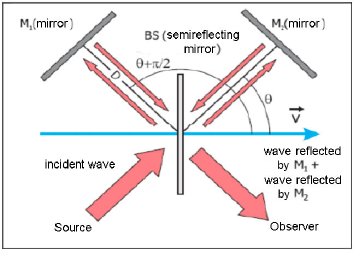
Figure 1: A schematic illustration of the Michelson interferometer.

This relation was at the base of the original Michelson interferometer but is also valid today when we assume Lorentz transformations. In this case, in fact, the length D, in the $S^{\prime}$ frame where the rod is at rest, is not depending on the orientation (in the last relation, we are assuming light propagation in a medium with a refractive index ${\cal N}=1+\epsilon$, and $\epsilon\ll 1$). We thus get the fringe patterns ($\lambda$ being the wavelength of light)

$${{\Delta\lambda(\theta)}\over{\lambda}}\sim{{2D}\over{\lambda}}~{}{{\Delta\bar{c}_{\theta}}\over{c}}$$ (5)

which were measured in the old experiments.

Instead, nowadays, an angular dependence of $\bar{c}_{\gamma}(\theta)$ is extracted from the frequency shift $\Delta\nu(\theta)$ of two optical resonators, see Fig.2. The particular type of laser-cavity coupling used in the experiments is known in the literature as the Pound-Drever-Hall system [53, 54]. The details of this technique go beyond our scopes. However, the main ideas are simple and beautifully explained in Black’s tutorial article [55]. A laser beam is sent into a Fabry-Perot cavity which acts as a filter. Then, a part of the output of the cavity is fed back to the laser to suppress its frequency fluctuations. This method provide a very narrow bandwidth and has been crucial for the precision measurements we are going to describe.

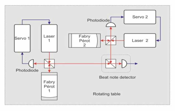
Figure 2: The scheme of a modern ether-drift experiment. The light frequencies are first stabilized by coupling the lasers to Fabry-Perot optical resonators. The frequencies $\nu_{1}$ and $\nu_{2}$ of the signals from the resonators are then compared in the beat note detector which provides the frequency shift $\Delta\nu=\nu_{1}-\nu_{2}$.

The frequency of the resonators is proportional to $\bar{c}_{\gamma}(\theta)$ through an integer number $m$, fixing the cavity mode, and the cavity length $L$ measured in the laboratory $S^{\prime}$ frame

$$\nu(\theta)={{\bar{c}_{\gamma}(\theta)m}\over{2L}}$$ (6)

Again, by assuming Lorentz transformations, the length of the cavity, in its rest frame $S^{\prime}$, does not depend on the orientation in space, so that

$${{\Delta\nu(\theta)}\over{\nu_{0}}}\sim{{\Delta\bar{c}_{\theta}}\over{c}}$$ (7)

$\nu_{0}$ being the reference frequency of the resonators. These relations have always been assumed in the interpretation of the experiments.

3. A modern version of Maxwell calculation

For a quantitative analysis, let us consider a medium of refractive index ${\cal N}=1+\epsilon$, with $0\leq\epsilon\ll 1$. This medium fills an optical cavity at rest in the laboratory $S^{\prime}$ frame in motion with velocity $v$ with respect to $\Sigma$. If we assume a) that $\bar{c}_{\gamma}(\theta)$ is isotropic when $S^{\prime}\equiv\Sigma$ and b) that Lorentz transformations are valid, then any anisotropy in $S^{\prime}$ should vanish identically either for $v=0$ or for the ideal vacuum limit, i.e. when the velocity of light tends to the basic parameter $c$ of Lorentz transformations . Therefore, one can perform an expansion in powers of the two small parameters $\epsilon$ and $\beta=v/c$. Since, by its definition, $\bar{c}_{\gamma}(\theta)$ is invariant under the replacement $\beta\to-\beta$ and, at fixed $\beta$, is invariant when replacing $\theta\to\pi+\theta$, the lowest non-trivial angular dependence is found to ${\cal O}(\epsilon\beta^{2})$ and can be expressed in the general form [17, 18, 19]

$$\bar{c}_{\gamma}(\theta)\sim{{c}\over{{\cal N}}}\left[1-\epsilon~{}\beta^{2}\sum^{\infty}_{n=0}\zeta_{2n}P_{2n}(\cos\theta)\right]$$ (8)

In the above relation, the invariance under $\theta\to\pi+\theta$ is achieved by expanding in even-order Legendre polynomials with arbitrary coefficients $\zeta_{2n}={\cal O}(1)$. These coefficients vanish identically in Einstein’s special relativity, with no preferred system, but should not vanish a priori in a “Lorentzian” formulation.

If we retain the first few $\zeta$’s as free parameters, Eq.(8) could already be useful for fitting experimental data. In any case, independently of their numerical values, one should appreciate the substantial difference introduced with respect to the classical prediction. As an example, by assuming for simplicity $v=$ 300 km/s, $\epsilon\sim 2.8\cdot 10^{-4}$ as for air at room temperature and atmospheric pressure, we find a difference

$$\frac{\Delta\bar{c}_{\theta}(0)}{c}\sim 2.8\cdot 10^{-10}\left[{{3}\over{2}}\zeta_{2}+{{5}\over{8}}\zeta_{4}+...\right]$$ (9)

This would be about three orders of magnitude smaller than the classical estimate $\beta^{2}=10^{-6}$, expected from Maxwell’s calculation [57], for the same $v=$ 300 km/s. However, depending on the actual $\zeta$’s, Eq.(9) would also be about 10$\div$ 20 times smaller than the old standard value for the much lower orbital velocity $v_{\rm orb}=$30 km/s

$$\frac{\Delta\bar{c}_{\theta}(0)}{c}\Big{|}_{\rm class}=\frac{v^{2}_{\rm orb}}{c^{2}}=10^{-8}$$ (10)

For experiments in gaseous helium at room temperature and atmospheric pressure, where $\epsilon\sim 3.3\cdot 10^{-5}$, the equivalent of Eq.(9) would even be $100\div 200$ times smaller than this old standard. The above elementary arguments suggest that the old ether-drift experiments in gaseous media might have been overlooked. So far, they have been considered as null results. But this may just depend on comparing with the wrong classical formula.

Yet, the dependence on the unknown $\zeta$’s is unpleasant because it prevents a straightforward comparison with the data. For this reason, by other symmetry arguments [37, 39, 40], we will further sharpen our analysis with another derivation of the $\epsilon\to 0$ limit. This additional derivation makes use of the effective space-time metric $g^{\mu\nu}=g^{\mu\nu}({\cal N})$ which should be replaced into the relation $g^{\mu\nu}p_{\mu}p_{\nu}=0$ to describe light in a medium of refractive index ${\cal N}$, see e.g. [58]. At the quantum level, this metric was derived by Jauch and Watson [59] when quantizing the electromagnetic field in a dielectric. They realized that the formalism introduces a preferred reference system where the photon energy $E_{\gamma}$ does not depend on the angle $\theta$ of light propagation. They observed that this is “usually taken as the system for which the medium is at rest”, a conclusion which is obvious in special relativity where there is no preferred system but less obvious in our case. We will therefore adapt their results and consider the different limit where the photon energy $E_{\gamma}$ is $\theta-$independent only when both medium and observer are at rest in some frame $\Sigma$.

To see how this works, we will consider two identical optical resonators, namely resonator 1, which is at rest in $\Sigma$, and resonator 2, which is at rest in $S^{\prime}$. We will also introduce $\pi_{\mu}\equiv({{E_{\pi}}\over{c}},{\bf\pi})$, to indicate the light 4-momentum for $\Sigma$ in his cavity 1, and $p_{\mu}\equiv({{E_{p}}\over{c}},{\bf p})$, to indicate the analogous 4-momentum of light for $S^{\prime}$ in his cavity 2. Finally we will define by $g^{\mu\nu}$ the space-time metric used by $S^{\prime}$ in the relation $g^{\mu\nu}p_{\mu}p_{\nu}=0$ and by

$$\gamma^{\mu\nu}={\rm diag}({\cal N}^{2},-1,-1,-1)$$ (11)

the metric which $\Sigma$ adopts in the analogous relation $\gamma^{\mu\nu}\pi_{\mu}\pi_{\nu}=0$ and which produces the isotropic velocity $c_{\gamma}=E_{\pi}/|{\bf\pi}|={{c}\over{{\cal N}}}$.

We emphasize the peculiar view of special relativity where no observable difference can exist between $\Sigma$ and $S^{\prime}$. In our perspective, instead, this physical equivalence is only assumed in the ideal ${\cal N}=1$ vacuum limit. Indeed, as anticipated in the Introduction, in the presence of matter, where light gets absorbed and then re-emitted, the fraction of refracted light could keep track of the particular motion of matter with respect to $\Sigma$ and produce a $\Delta\bar{c}_{\theta}\neq 0$.

By first considering the ${\cal N}=1$ limit, the frame-independence of the velocity of light requires to impose

$$g^{\mu\nu}({\cal N}=1)=\gamma^{\mu\nu}({\cal N}=1)=\eta^{\mu\nu}$$ (12)

where $\eta^{\mu\nu}$ is the Minkowski tensor. This standard equality amounts to introduce a transformation matrix, say $A^{\mu}_{\nu}$, such that, for ${\cal N}=1$

$$g^{\mu\nu}({\cal N}=1)=A^{\mu}_{\rho}A^{\nu}_{\sigma}\gamma^{\rho\sigma}({\cal N}=1)=A^{\mu}_{\rho}A^{\nu}_{\sigma}\eta^{\rho\sigma}=\eta^{\mu\nu}$$ (13)

This relation is strictly valid for ${\cal N}=1$. However, by continuity, one is driven to conclude that an analogous relation between $g^{\mu\nu}$ and $\gamma^{\mu\nu}$ should also hold in the $\epsilon\to 0$ limit. The only subtlety is that relation (13) does not fix uniquely $A^{\mu}_{\nu}$. In fact, it is fulfilled either by choosing the identity matrix, i.e. $A^{\mu}_{\nu}=\delta^{\mu}_{\nu}$, or by choosing a Lorentz transformation, i.e. $A^{\mu}_{\nu}=\Lambda^{\mu}_{\nu}$. It thus follows that $A^{\mu}_{\nu}$ is a two-valued function when ${\cal N}\to 1$.

This gives two possible solutions for the metric in $S^{\prime}$. In fact, when $A^{\mu}_{\nu}$ is the identity matrix, we find

$$\left[g^{\mu\nu}({\cal N})\right]_{1}=\delta^{\mu}_{\rho}\delta^{\nu}_{\sigma}\gamma^{\rho\sigma}=\gamma^{\mu\nu}\sim\eta^{\mu\nu}+2\epsilon\delta^{\mu}_{0}\delta^{\nu}_{0}$$ (14)

while, when $A^{\mu}_{\nu}$ is a Lorentz transformation, we obtain

$$\left[g^{\mu\nu}({\cal N})\right]_{2}=\Lambda^{\mu}_{\rho}\Lambda^{\nu}_{\sigma}\gamma^{\rho\sigma}\sim\eta^{\mu\nu}+2\epsilon v^{\mu}v^{\nu}$$ (15)

where $v_{\mu}$ is the $S^{\prime}$ 4-velocity, $v_{\mu}\equiv(v_{0},{\bf v}/c)$ with $v_{\mu}v^{\mu}=1$. As a consequence, the equality $\left[g^{\mu\nu}({\cal N})\right]_{1}=\left[g^{\mu\nu}({\cal N})\right]_{2}$ can only hold for $v^{\mu}=\delta^{\mu}_{0}$, i.e. for ${\bf v}=0$ when $S^{\prime}\equiv\Sigma$.

Notice that by choosing the first solution $\left[g^{\mu\nu}({\cal N})\right]_{1}$, which is implicitly assumed in special relativity to preserve isotropy in all reference frames also for ${\cal N}\neq 1$, we are considering a transformation matrix $A^{\mu}_{\nu}$ which is discontinuous for any $\epsilon\neq 0$. In fact, it is the non-trivial peculiarity of Lorentz transformations to enforce Eq.(13) for $A^{\mu}_{\nu}=\Lambda^{\mu}_{\nu}$ so that $\Lambda^{\mu\sigma}\Lambda^{\nu}_{\sigma}=\eta^{\mu\nu}$ and the Minkowski metric, if valid in one frame, will then apply to all equivalent frames.

On the other hand, if one inserts $\left[g^{\mu\nu}({\cal N})\right]_{2}$ in the relation $p_{\mu}p_{\nu}g^{\mu\nu}=0$, the photon energy $E(|{\bf{p}}|,\theta)$ will now depend on the direction of propagation. This gives the one-way velocity $c_{\gamma}(\theta)={{E(|{\bf{p}}|,\theta)}\over{|{\bf{p}}|}}$ which, to ${\cal O}(\epsilon)$ and ${\cal O}(\beta^{2})$, is

$$c_{\gamma}(\theta)\sim{{c}\over{{\cal N}}}~{}\left[1-2\epsilon\beta\cos\theta-\epsilon\beta^{2}(1+\cos^{2}\theta)\right]$$ (16)

with a two-way combination

$$\bar{c}_{\gamma}(\theta)={{2c_{\gamma}(\theta)c_{\gamma}(\pi+\theta)}\over{c_{\gamma}(\theta)+c_{\gamma}(\pi+\theta)}}\sim{{c}\over{{\cal N}}}~{}\left[1-\epsilon\beta^{2}(1+\cos^{2}\theta)\right]$$ (17)

This final form, corresponding to setting in Eq.(8) $\zeta_{0}=4/3$, $\zeta_{2}=2/3$ and all $\zeta_{2n}=0$ for $n>1$, could be considered the modern version of Maxwell’s calculation [57] and will be adopted in the analysis of experiments near the $\epsilon=0$ limit, as for gaseous systems.

For sake of clarity, let us return to the definition of the gas refractive index ${\cal N}$ in Eq.(11). How, is this quantity related to the experimental value ${\cal N}_{\rm exp}$ obtained from the two-way velocity measured in the earth laboratory? This can be easily understood by first introducing an angle-dependent $\bar{\cal N}(\theta)$ through $\bar{c}_{\gamma}(\theta)\equiv c/\bar{\cal N}(\theta)$ with

$$\bar{\cal N}(\theta)\sim{\cal N}~{}\left[1+({\cal N}-1)\beta^{2}(1+\cos^{2}\theta)\right]$$ (18)

and then defining the isotropic experimental value after an angular averaging, namely

$${{c}\over{{\cal N}_{\rm exp}}}\equiv\langle{{c}\over{\bar{\cal N}(\theta)}}\rangle_{\theta}={{c}\over{{\cal N}}}~{}\left[1-{{3}\over{2}}({\cal N}-1)\beta^{2}\right]$$ (19)

One could therefore obtain the unknown value ${\cal N}\equiv{\cal N}(\Sigma)$ (as if the cavity with the gas were at rest in $\Sigma$), from the experimental ${\cal N}_{\rm exp}\equiv{\cal N}(earth)$ and $v$. As an example, the most precise determinations for air are at a level $10^{-7}$, say ${\cal N}_{\rm exp}=1.0002924..$ for $\lambda=$ 589 nm, 0 ^oC and atmospheric pressure. Therefore, for $v\sim$ 370 km/s, the difference between ${\cal N}(\Sigma)$ and ${\cal N}(earth)$ is smaller than $10^{-9}$ and can be ignored. Analogous considerations apply to other gaseous media (as N, CO2, helium,..) where the precision in ${\cal N}_{\rm exp}$ is, at best, at the level of a few $10^{-7}$. Finally, whatever $v$, the relation ${\cal N}(\Sigma)={\cal N}_{\rm exp}$ becomes more and more accurate in the low-pressure limit where $({\cal N}_{\rm exp}-1)\to 0$.

To conclude, from Eq.(17) the fractional anisotropy is found to be

$${{\Delta\bar{c}_{\theta}}\over{c}}={{\bar{c}_{\gamma}(\pi/2+\theta)-\bar{c}_{\gamma}(\theta)}\over{c}}\sim\epsilon~{}{{v^{2}}\over{c^{2}}}\cos 2(\theta-\theta_{2})$$ (20)

and is suppressed by the small factor $2\epsilon$ with respect to the classical estimate ${{\Delta\bar{c}_{\theta}}\over{c}}\sim{{v^{2}}\over{2c^{2}}}$. Here $v$ and $\theta_{2}$ indicate the magnitude and the direction of the drift in the interferometer’s plane and, from Eq.(5), one obtains the fringe pattern

$${{\Delta\lambda(\theta)}\over{\lambda}}={{2D}\over{\lambda}}~{}{{\Delta\bar{c}_{\theta}}\over{c}}\sim{{2D}\over{\lambda}}~{}\epsilon~{}{{v^{2}}\over{c^{2}}}\cos 2(\theta-\theta_{2})$$ (21)

In this way, the dragging of light in the earth frame is described as a pure 2nd-harmonic effect which is periodic in the range $[0,\pi]$. This is the same as in the classical theory (see e.g. [60]), with the exception of its amplitude

$$A_{2}={{2D}\over{\lambda}}~{}\epsilon~{}{{{v}^{2}}\over{c^{2}}}$$ (22)

which is suppressed by the factor $2\epsilon$ relatively to the classical amplitude $A^{\rm class}_{2}={{D}\over{\lambda}}{{{v}^{2}}\over{c^{2}}}$. This difference could then be re-absorbed into an observable velocity

$$A_{2}={{D}\over{\lambda}}{{{v}^{2}_{\rm obs}}\over{c^{2}}}$$ (23)

which depends on the gas refractive index

$$v^{2}_{\rm obs}\sim 2\epsilon v^{2}$$ (24)

This $v_{\rm obs}$ is the very small velocity traditionally extracted from the classical analysis of the experiments through the relation

$$v_{\rm obs}\sim 30~{}{\rm km/s}~{}\sqrt{\frac{A^{\rm EXP}_{2}}{A^{\rm class}_{2}}}$$ (25)

when one was still comparing with the standard classical prediction $A^{\rm class}_{2}={{D}\over{\lambda}}(\frac{30~{}{\rm km/s}}{c})^{2}$ for the orbital velocity.

However, before a more detailed comparison with experiments, additional considerations are needed about the physical nature of the ether-drift as an irregular phenomenon. Some general motivations and a simple stochastic model will be illustrated in the following section.

4. Dragging of light as an irregular phenomenon

Besides the magnitude of the signal, the other important aspect of the experiments concerns the time dependence of the data. As anticipated in the Introduction, it was always assumed that, for short-time observations of a few days, where there are no sizeable changes in the orbital velocity of the earth, a genuine physical signal should reproduce the regular modulations induced by its rotation. The data instead, for both classical and modern experiments, have always shown a very irregular behavior with statistical averages much smaller than the instantaneous values. This was always a strong argument to interpret the data as instrumental artifacts. However, in principle, a definite instantaneous value ${{\Delta\bar{c}_{\theta}(t)}\over{c}}\neq 0$ could also coexist with a vanishing statistical average.

This possibility was considered in refs.[37] $-$ [42]by assuming that the observed signal is determined by a local velocity field, say $v_{\mu}(t)$, which does not coincide with the projection of the global earth motion, say $\tilde{v}_{\mu}(t)$, at the observation site. By comparing with the motion of a body in a fluid, the equality $v_{\mu}(t)=\tilde{v}_{\mu}(t)$ amounts to assume a form of regular, laminar flow where global and local velocity fields coincide. Instead, in the case of a turbulent fluid large-scale and small-scale flows would only be related indirectly.

An intuitive motivation for this turbulent-fluid analogy derives from comparing the vacuum to a fluid with vanishing viscosity. Then, within the Navier-Stokes equation, a laminar flow is by no means obvious due to the subtlety of the zero-viscosity (or infinite Reynolds number) limit, see for instance the discussion given by Feynman in Sect. 41.5, Vol.II of his Lectures [61]. The reason is that the velocity of such hypothetical fluid cannot be a differentiable function [62] and one should think, instead, in terms of a continuous, nowhere differentiable velocity field [63]. This analogy leads to the idea of a signal with a fundamental stochastic nature as when turbulence, at small scales, becomes homogeneous and isotropic.

With this in mind, let us return to Eq.(20) and make explicit the time dependence of the signal by re-writing as

$${{\Delta\bar{c}_{\theta}(t)}\over{c}}\sim\epsilon{{v^{2}(t)}\over{c^{2}}}\cos 2(\theta-\theta_{2}(t))$$ (26)

where $v(t)$ and $\theta_{2}(t)$ indicate respectively the instantaneous magnitude and direction of the drift in the plane of the interferometer. This can also be re-written as

$${{\Delta\bar{c}_{\theta}(t)}\over{c}}\sim 2{S}(t)\sin 2\theta+2{C}(t)\cos 2\theta$$ (27)

with

$$2C(t)=\epsilon~{}{{v^{2}_{x}(t)-v^{2}_{y}(t)}\over{c^{2}}}~{}~{}~{}~{}~{}~{}~{}2S(t)=\epsilon~{}{{2v_{x}(t)v_{y}(t)}\over{c^{2}}}$$ (28)

and $v_{x}(t)=v(t)\cos\theta_{2}(t)$, $v_{y}(t)=v(t)\sin\theta_{2}(t)$

The standard analysis is based on a cosmic velocity of the earth characterized by a magnitude $V$, a right ascension $\alpha$ and an angular declination $\gamma$. These parameters can be considered constant for short-time observations of a few days so that, with the traditional identifications $v(t)\equiv\tilde{v}(t)$ and $\theta_{2}(t)\equiv\tilde{\theta}_{2}(t)$, the only time dependence should be due to the earth rotation. Here $\tilde{v}(t)$ and $\tilde{\theta}_{2}(t)$ derive from the simple application of spherical trigonometry [64]

$$\cos z(t)=\sin\gamma\sin\phi+\cos\gamma\cos\phi\cos(t^{\prime}-\alpha)$$ (29)

$$\tilde{v}(t)=V\sin z(t)$$ (30)

$$\tilde{v}_{x}(t)=\tilde{v}(t)\cos\tilde{\theta}_{2}(t)=V\left[\sin\gamma\cos\phi-\cos\gamma\sin\phi\cos(t^{\prime}-\alpha)\right]$$ (31)

$$\tilde{v}_{y}(t)=\tilde{v}(t)\sin\tilde{\theta}_{2}(t)=V\cos\gamma\sin(t^{\prime}-\alpha)$$ (32)

In the above relations, $z=z(t)$ is the zenithal distance of ${\bf{V}}$, $\phi$ is the latitude of the laboratory, $t^{\prime}=\omega_{\rm sid}t$ is the sidereal time of the observation in degrees ($\omega_{\rm sid}\sim{{2\pi}\over{23^{h}56^{\prime}}}$) and the angle $\tilde{\theta}_{2}(t)$ is counted conventionally from North through East so that North is $\tilde{\theta}_{2}=0$ and East is $\tilde{\theta}_{2}=90^{o}$. With the identifications $v(t)\equiv\tilde{v}(t)$ and $\theta_{2}(t)\equiv\tilde{\theta}_{2}(t)$ (or equivalently $v_{x}(t)=\tilde{v}_{x}(t)$ and $v_{y}(t)=\tilde{v}_{y}(t)$) one thus arrives to the simple Fourier decomposition

$$S(t)\equiv\tilde{S}(t)=S_{0}+{S}_{s1}\sin t^{\prime}+{S}_{c1}\cos t^{\prime}+{S}_{s2}\sin(2t^{\prime})+{S}_{c2}\cos(2t^{\prime})$$ (33)

$$C(t)\equiv\tilde{C}(t)={C}_{0}+{C}_{s1}\sin t^{\prime}+{C}_{c1}\cos t^{\prime}+{C}_{s2}\sin(2t^{\prime})+{C}_{c2}\cos(2t^{\prime})$$ (34)

where the $C_{k}$ and $S_{k}$ Fourier coefficients depend on the three parameters $(V,\alpha,\gamma)$ and are given explicitly in refs.[37, 40].

Instead, we will consider an alternative scenario where $v_{x}(t)\neq\tilde{v}_{x}(t)$ and $v_{y}(t)\neq\tilde{v}_{y}(t)$. In particular the local velocity components, $v_{x}(t)$ and $v_{y}(t)$, will be assumed to be non-differentiable functions expressed in terms of random Fourier series [62, 65, 66]. The simplest model corresponds to a turbulence which, at small scales, appears homogeneous and isotropic. The analysis of the previous section, can then be embodied in an effective space-time metric for light propagation

$$g^{\mu\nu}(t)\sim\eta^{\mu\nu}+2\epsilon v^{\mu}(t)v^{\nu}(t)$$ (35)

where $v_{\mu}(t)$ is a random 4-velocity field which describes the drift and whose boundaries depend on the smooth $\tilde{v}_{\mu}(t)$ determined by the average motion of the earth. If this corresponds to the actual physical situation, a genuine stochastic signal can easily become consistent with average values $(C_{k})^{\rm avg}=(S_{k})^{\rm avg}=0$ obtained by fitting the data with Eqs.(33) and (34).

For homogeneous turbulence a series representation, suitable for numerical simulations of a discrete signal, can be expressed in the form

$$v_{x}(t_{k})=\sum^{\infty}_{n=1}\left[x_{n}(1)\cos\omega_{n}t_{k}+x_{n}(2)\sin\omega_{n}t_{k}\right]$$ (36)

$$v_{y}(t_{k})=\sum^{\infty}_{n=1}\left[y_{n}(1)\cos\omega_{n}t_{k}+y_{n}(2)\sin\omega_{n}t_{k}\right]$$ (37)

Here $\omega_{n}=2n\pi/T$ and T is the common period of all Fourier components. Furthermore, $t_{k}=(k-1)\Delta t$, with $k=1,2...$, and $\Delta t$ is the sampling time. Finally, $x_{n}(i=1,2)$ and $y_{n}(i=1,2)$ are random variables with the dimension of a velocity and vanishing mean.

In our simulations, the value $T=T_{\rm day}$= 24 hours and a sampling step $\Delta t=$ 1 second were adopted. However, the results would remain unchanged by any rescaling $T\to sT$ and $\Delta t\to s\Delta t$.

In general, we define $[-d_{x}(t),d_{x}(t)]$ the range for $x_{n}(i=1,2)$ and by $[-d_{y}(t),d_{y}(t)]$ the corresponding range for $y_{n}(i=1,2)$. By assuming statistical isotropy we should impose $d_{x}(t)=d_{y}(t)$. However, to see the difference, we will first consider the more general case $d_{x}(t)\neq d_{y}(t)$. If we assume that $x_{n}(i=1,2)$ and $y_{n}(i=1,2)$ vary with uniform probability within their ranges $[-d_{x}(t),d_{x}(t)]$ and $[-d_{y}(t),d_{y}(t)]$, the only non-vanishing (quadratic) statistical averages are

$$\langle x^{2}_{n}(i=1,2)\rangle_{\rm stat}={{d^{2}_{x}(t)}\over{3~{}n^{2\eta}}}~{}~{}~{}~{}~{}~{}~{}~{}~{}~{}~{}\langle y^{2}_{n}(i=1,2)\rangle_{\rm stat}={{d^{2}_{y}(t)}\over{3~{}n^{2\eta}}}$$ (38)

Here, the exponent $\eta$ ensures finite statistical averages $\langle v^{2}_{x}(t)\rangle_{\rm stat}$ and $\langle v^{2}_{y}(t)\rangle_{\rm stat}$ for an arbitrarily large number of Fourier components. In our simulations, between the two possible alternatives $\eta=5/6$ and $\eta=1$ of ref.[66], we have chosen $\eta=1$ that corresponds to the Lagrangian picture in which the point where the fluid velocity is measured is a wandering material point in the fluid.

In the end, the cosmic motion of the earth enters through the identifications $d_{x}(t)=\tilde{v}_{x}(t)$ and $d_{y}(t)=\tilde{v}_{y}(t)$ as defined in Eqs.(29)$-$(32) with $V=$ 370 km/s, $\alpha=168$ degrees, $\gamma=-$ 7 degrees, as fixed from our motion within the CMB.

On the other hand, by assuming statistical isotropy, from the relation

$$\tilde{v}^{2}_{x}(t)+\tilde{v}^{2}_{y}(t)=\tilde{v}^{2}(t)$$ (39)

we obtain the identification

$$d_{x}(t)=d_{y}(t)={{\tilde{v}(t)}\over{\sqrt{2}}}$$ (40)

For this isotropic model, from Eqs.(36)$-$(40), we find

$$\langle v^{2}_{x}(t)\rangle_{\rm stat}=\langle v^{2}_{y}(t)\rangle_{\rm stat}={{\tilde{v}^{2}(t)}\over{2}}~{}{{1}\over{3}}\sum^{\infty}_{n=1}{{1}\over{n^{2}}}={{\tilde{v}^{2}(t)}\over{2}}~{}{{\pi^{2}}\over{18}}$$

$$\langle v_{x}(t)v_{y}(t)\rangle_{\rm stat}=0$$ (41)

with statistical averages for the functions Eqs.(28)

$$\langle C(t)\rangle_{\rm stat}=0~{}~{}~{}~{}~{}~{}~{}~{}~{}~{}~{}~{}~{}~{}~{}~{}~{}~{}\langle S(t)\rangle_{\rm stat}=0$$ (42)

which vanish at any time $t$. Therefore this model describes a definite non-zero signal but, if this signal were now fitted with Eqs.(33) and (34), it would produce vanishing averages $(C_{k})^{\rm avg}=0$, $(S_{k})^{\rm avg}=0$ for all Fourier coefficients. In other words, with such physical signal, these statistical averages will become smaller and smaller by simply increasing the number of observations.

5. The classical experiments in gaseous media

To understand how radical is the modification produced by Eqs.(42) in the analysis of the data, let us now consider the traditional procedure adopted in the classical experiments. One was measuring the fringe shifts at some given sidereal time on consecutive days so that changes of the orbital velocity were negligible. Then, see Eqs.(21) and (27), the measured shifts at the various angle $\theta$ were averaged

$$\langle{{\Delta\lambda(\theta;t)}\over{\lambda}}\rangle_{\rm stat}={{2D}\over{\lambda}}\left[2\sin 2\theta~{}\langle S(t)\rangle_{\rm stat}+2\cos 2\theta~{}\langle C(t)\rangle_{\rm stat}\right]$$ (43)

and finally these average values were compared with models for the earth cosmic motion.

However if, following the arguments of the previous section, the signal is so irregular that, by increasing the number of measurements, $\langle C(t)\rangle_{\rm stat}\to 0$ and $\langle S(t)\rangle_{\rm stat}\to 0$ the averages Eq.(43) would have no meaning. In fact, these averages would be non vanishing just because the statistics is finite. In particular, the direction $\theta_{2}(t)$ of the drift (defined by the relation $\tan 2\theta_{2}(t)=S(t)/C(t)$) would vary randomly with no definite limit.

Table 1: The 2nd-harmonic amplitudes for the six experimental sessions of the Michelson-Morley experiment. The table is taken from ref.[37].

SESSION	$A^{\rm EXP}_{2}$
July 8 (noon)	$0.010\pm 0.005$
July 9 (noon)	$0.015\pm 0.005$
July 11 (noon)	$0.025\pm 0.005$
July 8 (evening)	$0.014\pm 0.005$
July 9 (evening)	$0.011\pm 0.005$
July 12 (evening)	$0.024\pm 0.005$

Therefore, we should concentrate the analysis on the 2nd-harmonic amplitudes

$$A_{2}(t)={{2D}\over{\lambda}}~{}2\sqrt{S^{2}(t)+C^{2}(t)}\sim{{2D}\over{\lambda}}~{}\epsilon{{v^{2}_{x}(t)+v^{2}_{y}(t)}\over{c^{2}}}$$ (44)

which are positive-definite and remain non-zero under the averaging procedure. Moreover, these are rotational-invariant quantities and their statistical properties would remain unchanged in the isotropic model Eq.(40) or with the alternative choice $d_{x}(t)\equiv\tilde{v}_{x}(t)$ and $d_{y}(t)\equiv\tilde{v}_{y}(t)$. In this way, in a smooth deterministic model and using Eq.(30), we obtain

$$\tilde{A}_{2}(t)\sim{{2D}\over{\lambda}}\cdot\epsilon{{\tilde{v}^{2}(t)}\over{c^{2}}}\sim{{2D}\over{\lambda}}\cdot\epsilon{{V^{2}}\over{c^{2}}}\cdot\sin^{2}z(t)$$ (45)

while, with a full statistical average, from Eq.(4.)

$$\langle A_{2}(t)\rangle_{\rm stat}\sim{{\pi^{2}}\over{18}}\cdot\tilde{A}_{2}(t)$$ (46)

By comparing these two expressions, it is evident that, from the same data, one would now get a velocity which is larger by a factor $\sqrt{18/\pi^{2}}\sim$ 1.35. Also, from Eq.(30), besides the average magnitude $\langle\tilde{v}^{2}(t)\rangle_{\rm day}=V^{2}\langle\sin^{2}z(t)\rangle_{\rm day}$, one could determine the angular parameters $\alpha$ and $\gamma$ from the time modulations of the amplitude.

As an example, let us consider the 2nd-harmonic amplitudes for the Michelson-Morley experiment, see Table 1. From these data, by computing mean and variance, one finds $\langle A^{\rm EXP}_{2}\rangle\sim 0.016\pm 0.006$ so that by comparing with the classical prediction $A^{\rm class}_{2}={{D}\over{\lambda}}{{(30{\rm km/s})^{2}}\over{c^{2}}}\sim 0.20$ and using Eq.(25), we find an observable velocity $v_{\rm obs}\sim(8.4\pm 1.6)$ km/s in good agreement with Miller’s analysis, see Fig.3. However, for air at atmospheric pressure where $\epsilon\sim 2.8\cdot 10^{-4}$, the true kinematical value would instead be $\tilde{v}\sim(355\pm 70)$ km/s from Eq.(45) or $\tilde{v}\sim(480\pm 95)$ km/s from Eq.(46).

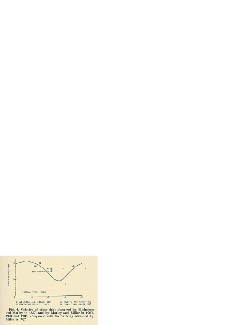
Figure 3: The observable velocity measured in various experiments as reported by Miller [27].

Let us then consider Miller’s very extensive observations. After the re-analysis of his work by the Shankland team [45], there is now the average 2nd harmonic $\langle A^{\rm EXP}_{2}\rangle=0.044\pm 0.022$ for all epochs of the year (see Table III of [45]). By comparing this amplitude with the classical prediction for Miller’s apparatus $A^{\rm class}_{2}={{D}\over{\lambda}}{{(30{\rm km/s})^{2}}\over{c^{2}}}\sim 0.56$, we find $v_{\rm obs}\sim(8.4\pm 2.2)$ km/s. However, the true kinematical velocity is instead $\tilde{v}\sim(355\pm 70)$ km/s from Eq.(45) or $\tilde{v}\sim(480\pm 95)$ km/s from Eq.(46).

Note the agreement of two determinations obtained in very different conditions (the basement of Cleveland laboratory or the top of Mount Wilson). This shows that the traditional interpretation [44, 45] of the residuals as temperature differences in the optical paths is only acceptable provided these temperature differences have a non-local origin. We will return to this point in Section 6.

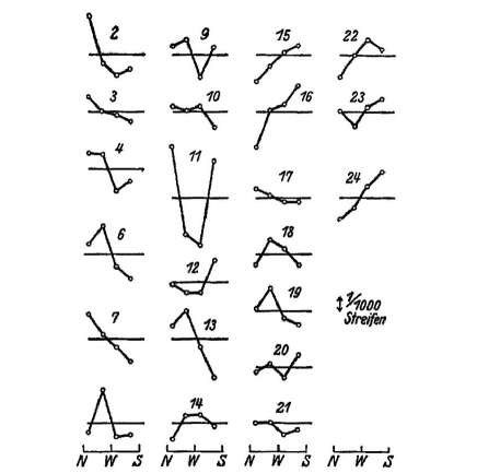
Figure 4: The fringe shifts reported by Joos [35]. The yardstick corresponds to 1/1000 of a wavelength.

There is no space for the details of all classical experiments. For that, we address the reader to our book [40] which also contains many historical notes and references to previous works. Here we will only limit ourselves to a brief description of Joos’ 1930 experiment [35] in Jena (sensitivity of about 1/3000 of a fringe) which is, by far, the most precise of the classical repetitions of the Michelson-Morley experiment and is considered the definitive disproof of Miller’s claims of a non-zero effect .

The data were taken at intervals of one hour during the sidereal day and recorded photographically with an automatic procedure, see Fig.4. From this picture, Joos adopted 1/1000 of a wavelength as upper limit and deduced the bound $v_{\rm obs}\lesssim 1.5$ km/s. To this end, he was comparing with the classical expectation that, for his apparatus, a velocity of 30 km/s should have produced a 2nd-harmonic amplitude of 0.375 wavelengths. Though, since it is apparent that some fringe displacements were certainly larger than 1/1000 of a wavelength, we have performed 2nd-harmonic fits to Joos’ data, see Fig.5. The resulting amplitudes are reported in Fig.6.

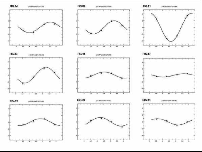
Figure 5: Some 2nd-harmonic fits to Joos’ data. The figure is taken from ref.[40].

Figure 6: Joos’ 2nd-harmonic amplitudes, in units $10^{-3}$. The vertical band between the two lines corresponds to the range $(1.4\pm 0.8)\cdot 10^{-3}$. The figure is taken from ref.[37].

We note that a 2nd-harmonic fit to the large fringe shifts in picture 11 has a very good chi-square, comparable and often better than other observations with smaller values, see Fig.5. Therefore, there is no reason to delete the observation n.11. Its amplitude, however, is more than ten times larger than the amplitudes from observations 20 and 21. This difference cannot be understood in a smooth model of the drift where the projected velocity squared at the observation site can at most differ by a factor of two, as for the CMB motion at typical Central-Europe latitude where $(\tilde{v})_{\rm min}\sim 250$ km/s and $(\tilde{v})_{\rm max}\sim 370$ km/s. To understand these characteristic fluctuations, we have thus performed various numerical simulations of these amplitudes [37, 40] in our stochastic model. To this end, Eqs.(36) and (37) were replaced in Eq.(44) and the random velocity components were bounded by the kinematical parameters $(V,\alpha,\gamma)_{\rm CMB}$ as explained in Sect.4. Two simulations are shown in Figs.7 and 8.

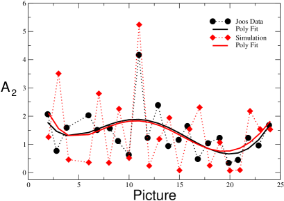
Figure 7: Joos’ 2nd-harmonic amplitudes, in units $10^{-3}$ (black dots), are compared with a single simulation (red diamonds) at the same sidereal times of Joos’ observations. Two 5th-order polynomial fits to the two sets of values are also shown. The figure is taken from ref.[37] .

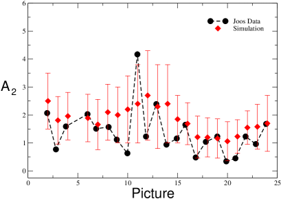
Figure 8: Joos’ 2nd-harmonic amplitudes in units $10^{-3}$ (black dots) are now compared with a simulation where one averages ten measurements, performed on 10 consecutive days, at the same sidereal times of Joos’ observations (red diamonds). The change of the averages observed by varying the parameters of the simulation was summarized into a central value and a symmetric error. The figure is taken from ref.[37].

We want to emphasize two aspects. First, Joos’ average amplitude $\langle A^{\rm EXP}_{2}\rangle=(1.4\pm 0.8)\cdot 10^{-3}$ when compared with the classical prediction for his interferometer $A^{\rm class}_{2}={{D}\over{\lambda}}{{(30{\rm km/s})^{2}}\over{c^{2}}}\sim 0.375$ gives indeed an observable velocity $v_{\rm obs}\sim(1.8\pm 0.5)$ km/s very close to the $1.5$ km/s value quoted by Joos. But, when comparing with our prediction in the stochastic model Eq.(46) one would now find a true kinematical velocity $\tilde{v}=305^{+85}_{-100}$ km/s. Second, when fitting with Eqs.(29) and (30) the smooth black curve of the Joos data in Fig.7 one finds [37] a right ascension $\alpha({\rm fit-Joos})=(168\pm 30)$ degrees and an angular declination $\gamma({\rm fit-Joos})=(-13\pm 14)$ degrees which are consistent with the present values $\alpha({\rm CMB})\sim$ 168 degrees and $\gamma({\rm CMB})\sim-$7 degrees. This confirms that, when studied at different sidereal times, the measured amplitude can also provide precious information on the angular parameters.

Finally, all experiments are compared with our stochastic model Eq.(46) in Table 2. Notice the substantial difference with the analogous summary Table I of ref.[45] where those authors were comparing with the classical relation $A^{\rm class}_{2}={{D}\over{\lambda}}{{(30{\rm km/s})^{2}}\over{c^{2}}}$ and emphasizing the much smaller magnitude of the experimental data. Here, is just the opposite. In fact, our theoretical estimates are often smaller than the experimental results indicating, most likely, the presence of systematic effects in the measurements. At the same time, however, by adopting Eq.(46), the experiments in air give $\tilde{v}_{\rm air}\sim 418\pm 62$ km/s and the two experiments in gaseous helium $\tilde{v}_{\rm helium}\sim 323\pm 70$ km/s, with a global average $\langle\tilde{v}\rangle\sim 376\pm 46$ km/s which agrees well with the 370 km/s from the direct CMB observations. Even more, from the most precise Piccard-Stahel and Joos experiments we find two determinations, $\tilde{v}=360^{+85}_{-110}$ km/s and $\tilde{v}=305^{+85}_{-100}$ km/s respectively, whose average $\langle\tilde{v}\rangle\sim 332^{+60}_{-80}$ km/s reproduces to high accuracy the projection of the CMB velocity at a typical Central-Europe latitude .

Table 2: The average 2nd-harmonic amplitudes of classical ether-drift experiments. These were extracted from the original papers by averaging the amplitudes of the individual observations and assuming the direction of the local drift to be completely random (i.e. no vector averaging of different sessions). These experimental values are then compared with the full statistical average Eq.(46) for a projection of the velocity 250 km/s $\leq{\tilde{v}}(t)\leq$ 370 km/s and refractivities $\epsilon=2.8\cdot 10^{-4}$ for air and $\epsilon=3.3\cdot 10^{-5}$ for gaseous helium. The experimental value for the Morley-Miller experiment is taken from the observed velocities reported in Miller’s Figure 4, here our Fig.3. The experimental value for the Michelson-Pease-Pearson experiment refers to the only known session for which the fringe shifts are reported explicitly [34] and where the optical path was still fifty-five feet. The symbol $\pm....$ means that the experimental uncertainty cannot be determined from the available informations.

Experiment	gas	$A^{\rm EXP}_{2}$	${{2D}\over{\lambda}}$	$\langle A_{2}(t)\rangle_{\rm stat}$
Michelson(1881)	air	$(7.8\pm....)\cdot 10^{-3}$	$4\cdot 10^{6}$	$(0.7\pm 0.2)\cdot 10^{-3}$
Michelson-Morley(1887)	air	$(1.6\pm 0.6)\cdot 10^{-2}$	$4\cdot 10^{7}$	$(0.7\pm 0.2)\cdot 10^{-2}$
Morley-Miller(1902-1905)	air	$(4.0\pm 2.0)\cdot 10^{-2}$	$1.12\cdot 10^{8}$	$(2.0\pm 0.7)\cdot 10^{-2}$
Miller(1921-1926)	air	$(4.4\pm 2.2)\cdot 10^{-2}$	$1.12\cdot 10^{8}$	$(2.0\pm 0.7)\cdot 10^{-2}$
Tomaschek (1924)	air	$(1.0\pm 0.6)\cdot 10^{-2}$	$3\cdot 10^{7}$	$(0.5\pm 0.2)\cdot 10^{-2}$
Kennedy(1926)	helium	$<0.002$	$7\cdot 10^{6}$	$(1.4\pm 0.5)\cdot 10^{-4}$
Illingworth(1927)	helium	$(2.2\pm 1.7)\cdot 10^{-4}$	$7\cdot 10^{6}$	$(1.4\pm 0.5)\cdot 10^{-4}$
Piccard-Stahel(1928)	air	$(2.8\pm 1.5)\cdot 10^{-3}$	$1.28\cdot 10^{7}$	$(2.2\pm 0.8)\cdot 10^{-3}$
Mich.-Pease-Pearson(1929)	air	$(0.6\pm....)\cdot 10^{-2}$	$5.8\cdot 10^{7}$	$(1.0\pm 0.4)\cdot 10^{-2}$
Joos(1930)	helium	$(1.4\pm 0.8)\cdot 10^{-3}$	$7.5\cdot 10^{7}$	$(1.5\pm 0.6)\cdot 10^{-3}$

These non-trivial checks confirm the overall consistency of our picture with the classical experiments and should induce to perform new dedicated experiments where the optical resonators which are coupled to the lasers (see Fig.2) are filled by gaseous media. In this case, from Eq.(7), one should compare the data with the prediction

$${{\Delta\nu(\theta)}\over{\nu_{0}}}={{\Delta\bar{c}_{\theta}}\over{c}}\sim\epsilon~{}{{v^{2}}\over{c^{2}}}\cos 2(\theta-\theta_{2})$$ (47)

However, precise measurements of the frequency shift in the gas mode are not so simple [70]. For this reason, it is unclear if there will be a definite improvement with respect to the classical experiments, in particular with respect to Piccard-Stahel and Joos.

At present, a rough check of Eq.(47) can however be obtained from the variations of the signal observed in the only modern experiment that was performed in these conditions: the 1963 experiment by Jaseja et.al [71] with He-Ne lasers. Actually, at that time, optical resonators were not yet used and thus they were comparing directly the frequencies of two orthogonal He-Ne lasers under 90 degrees rotations of the apparatus. But the light from the lasers was emerging from a He-Ne gas mixture and thus the laser frequencies were providing a measure of the two-way velocity of light in that environment. As a matter of fact, for a laser frequency $\nu_{0}\sim 2.6\cdot 10^{14}$ Hz, after subtracting a large systematic effect of about 270 kHz due to magnetostriction, the residual variations of a few kHz are roughly consistent with the refractive index ${\cal N}_{\rm He-Ne}\sim 1.00004$ and the typical change of the cosmic velocity of the earth for the latitude of Boston. For more details, see the discussion given in [38, 40].

6. Experiments in gases vs. vacuum and solid dielectrics

The results in Table 2 support the idea of a tiny ${{\Delta\bar{c}_{\theta}}\over{c}}$ at the level $10^{-10}$ for the experiments in air and $10^{-11}$ for those in gaseous helium. Simple symmetry arguments suggest the relation ${{\Delta\bar{c}_{\theta}}\over{c}}\sim({\cal N}_{\rm gas}-1){{v^{2}}\over{c^{2}}}$ so that, from the data, we find the typical velocity $v\sim$ 300 km/s expected from our motion within the CMB. But, yet, one could ask: apart from symmetry arguments, how is the earth motion producing this small observed anisotropy in the gaseous systems?

As a possible hint, we recall that Eq.(8) was originally deduced in [18] as the most general angular dependence of the refractive index in the presence of convective currents of the gas molecules generated by an earth velocity $v$. This idea of convection, with respect to the container of the gas at rest in the laboratory, leads to reconsider the traditional explanation of the small residuals in terms of tiny temperature differences of a millikelvin or so [44, 45]. The interesting aspect is that, besides helping our intuition, this thermal interpretation will, in the end, be useful to analyze the complementary region of solid dielectrics where the refractive index ${\cal N}$ is very different from unity.

In principle, as anticipated in the Introduction, with angular differences $\Delta T^{\rm CMB}(\theta)=\pm$ 3.36  mK of the background radiation Eq.(2), temperature differences of this magnitude could reflect the collisions of the gas molecules, with mean velocity of 370 km/s, with the CMB-photons. These collisions could bring the gas out of equilibrium and induce a temperature difference $\Delta T^{\rm gas}(\theta)$ in the optical paths. In general, one expects $\Delta T^{\rm gas}(\theta)\leq\Delta T^{\rm CMB}(\theta)$, the two extreme cases $\Delta T^{\rm gas}(\theta)=0$ and $\Delta T^{\rm gas}(\theta)=\Delta T^{\rm CMB}(\theta)$ corresponding respectively to the limits of vanishing interactions or a very strong coupling of the two systems.

In view of the complexity of the calculation, we have not attempted a full microscopic derivation of the effect but just limited ourselves to a much simpler thermodynamic analysis [39, 40]. This just assumes the existence of some $\Delta T^{\rm gas}(\theta)$ to derive a corresponding difference in the refractive index in the optical paths. Consistency with the idea of a non-local effect will then require the same average $\langle\Delta T^{\rm gas}(\theta)\rangle$ from different experiments.

This type of analysis starts from the Lorentz-Lorenz equation

$${{{\cal N}^{2}-1}\over{{\cal N}^{2}+2}}=A_{R}\rho+B_{R}\rho^{2}...$$ (48)

where $\rho$ is the molar density and $A_{R}=(4/3)\pi N_{A}\alpha$ is the product of the Avogadro number $N_{A}$ and of the molecular polarizability $\alpha$ (see e.g. [70]). The coefficient $B_{R}$ takes into account two-body interactions which, for air and helium at atmospheric pressure, can be ignored. For ${\cal N}\sim 1$ we thus obtain the relation for the gas refractivity

$$\epsilon={\cal N}-1\sim{{3}\over{2}}A_{R}\rho$$ (49)

In the ideal-gas approximation, the molar density at STP (atmospheric pressure and $T=$ 273.15 K) has the value

$$\rho(STP)={{P}\over{RT}}={{101325}\over{(8.314)(273.15)}}~{}{\rm mol}\cdot{\rm m}^{-3}\sim 4.46\cdot 10^{-5}~{}{\rm mol}\cdot{\rm cm}^{-3}$$ (50)

As an example, for helium and a wavelength $\lambda=$ 633 nm, where $\alpha\sim 0.52~{}{\rm mol}^{-1}\cdot{\rm cm}^{3}$ [70], this gives $\epsilon\sim 3.5\cdot 10^{-5}$. Thus, in this simple approximation, where the temperature dependence of $\epsilon$ is

$$-{{\partial\epsilon}\over{\partial T}}\sim{{3}\over{2}}A_{R}{{P}\over{RT^{2}}}\sim{{\epsilon}(T)\over{T}}$$ (51)

and from the relation $\bar{c}_{\gamma}(\theta)\equiv{{c}\over{\bar{\cal N}(\theta)}}$, a difference $\Delta T^{\rm gas}(\theta)$ is seen to induce a typical angular difference

$${{|\Delta\bar{c}_{\theta}|}\over{c}}\sim~{}|\bar{\cal N}(\theta)-\bar{\cal N}(\pi/2+\theta)|\sim{{~{}\epsilon(T)|\Delta T^{\rm gas}(\theta)|}\over{T}}$$ (52)

which should be visible in the fringe shifts with a 2nd-harmonic amplitude

$$A^{\rm exp}_{2}\sim{{2D}\over{\lambda}}~{}{{\epsilon(T)|\Delta T^{\rm gas}(\theta)|}\over{T}}$$ (53)

For an average room temperature $T\sim 288\div 293$ K of the experiments, the values of $|\Delta T^{\rm gas}(\theta)|$ are reported in Table 3 for those cases where one can determine a meaningful experimental uncertainty.

Table 3: The average 2nd-harmonic amplitude observed in various classical ether-drift experiments and the resulting temperature difference (in mK) from Eq.(53).

Experiment	gas	$A^{\rm EXP}_{2}$	${{2D}\over{\lambda}}$	$|\Delta T^{\rm gas}(\theta)|$
Michelson-Morley(1887)	air	$(1.6\pm 0.6)\cdot 10^{-2}$	$4\cdot 10^{7}$	$0.40\pm 0.15$
Miller(1925-1926)	air	$(4.4\pm 2.2)\cdot 10^{-2}$	$1.12\cdot 10^{8}$	$0.39\pm 0.20$
Illingworth(1927)	helium	$(2.2\pm 1.7)\cdot 10^{-4}$	$7\cdot 10^{6}$	$0.29\pm 0.22$
Tomaschek (1924)	air	$(1.0\pm 0.6)\cdot 10^{-2}$	$3\cdot 10^{7}$	$0.33\pm 0.20$
Piccard-Stahel(1928)	air	$(2.8\pm 1.5)\cdot 10^{-3}$	$1.28\cdot 10^{7}$	$0.22\pm 0.12$
Joos(1930)	helium	$(1.4\pm 0.8)\cdot 10^{-3}$	$7.5\cdot 10^{7}$	$0.17\pm 0.10$

The very good chi-square, 2.4/(6-1)=0.48, shows that all experiments, can become consistent with the same average value

$$\langle\Delta T^{\rm exp}(\theta)\rangle=(0.26\pm 0.06)~{}{\rm mK}$$ (54)

so that the residuals observed in the old experiments could also be interpreted as thermal effects of non-local origin .

This previous analysis suggests two considerations. First, the old estimates of about 1 mK by Kennedy, Shankland and Joos (see [44, 45]) were slightly too large. Within our present view, this may indicate that the interactions of the gas molecules with the CMB photons are so weak that, on average, only less than 1/10 of $\Delta T^{\rm CMB}(\theta)$ is transferred to the gas in the optical paths. Second, with the thermal mechanism discussed above, one could replace in Eq.(18) $\epsilon_{\rm gas}=({\cal N}_{\rm gas}-1)\equiv\epsilon_{\rm thermal}+\epsilon_{v}$ and re-write

$${{\bar{\cal N}_{\rm gas}(\theta)}\over{{\cal N}_{\rm gas}}}\sim 1+(\epsilon_{\rm thermal}+\epsilon_{v})\beta^{2}(1+\cos^{2}\theta)$$ (55)

where $\epsilon_{\rm thermal}\equiv({\cal N}_{\rm gas}-{\cal N}_{v})$, $\epsilon_{v}\equiv({\cal N}_{v}-1)$. In this way, we have introduced an extremely small quantity $\epsilon_{v}$ which, in principle, could still account for a difference between the velocity of light $c_{\gamma}\equiv c/{\cal N}_{v}$, as measured in vacuum on the earth surface, and the ideal parameter $c$ of Lorentz transformations.

To roughly estimate a possible non-zero $\epsilon_{v}$, let us first recall that today the (isotropic) speed of light in vacuum is a reference standard with zero error, namely $c_{\rm ref}=$ 299 792 458 m/s and that the last precision measurements, performed before fixing this reference value, had an error of about 1 m/s at the 3-sigma level [75]. Therefore assuming $|c-c_{\rm ref}|\lesssim$ 1 m/s, we would tentatively estimate $\epsilon_{v}\lesssim 10^{-9}$. As such, at room temperature and atmospheric pressure, where this $\epsilon_{v}$ is numerically irrelevant, $\epsilon_{\rm thermal}$ is practically the same refractive index considered so far, i.e. $\epsilon_{\rm air}\sim 2.8\cdot 10^{-4}$ or $\epsilon_{\rm helium}\sim 3.3\cdot 10^{-5}$. Nevertheless Eq.(55) is useful because, in the opposite limit of an extremely high vacuum where now $\epsilon_{\rm thermal}=0$, for $\epsilon_{v}\neq 0$, we would predict the angular dependence

$${{\bar{\cal N}_{v}(\theta)}\over{{\cal N}_{v}}}\sim 1+\epsilon_{v}\beta^{2}(1+\cos^{2}\theta)$$ (56)

and an anisotropy of the two-way velocity of light in vacuum

$${{\Delta\bar{c}_{\theta}}\over{c}}\Big{|}_{\rm vacuum}=\bar{\cal N}_{v}(\theta)-\bar{\cal N}_{v}(\pi/2+\theta)~{}\sim~{}\epsilon_{v}\beta^{2}\cos 2\theta$$ (57)

Even more interestingly, the thermal argument is also useful to analyze experiments in solid dielectrics, as that originally performed by Shamir and Fox [43] in 1969. They were aware that the Michelson-Morley experiment did not yield a strictly zero result: “The non-zero result might have been real and due to the fact that the experiment was performed in air and not in vacuum” [43]. Therefore, within the traditional Lorentz-contraction interpretation of the experiment, with a refractive index ${\cal N}$ substantially above unity, one might expect a large ${{|\Delta\bar{c}_{\theta}|}\over{c}}\sim({\cal N}^{2}-1)\beta^{2}\sim\beta^{2}\sim 10^{-6}$. This was the motivation for their experiment in perspex (${\cal N}=1.5$). Since their measurements were orders of magnitude smaller, they concluded that the experimental basis of special relativity was strengthened.

However, with a thermal interpretation of the residuals in gaseous media, the two different behaviors can coexist. In fact, as anticipated in the Introduction, in a strongly bound system as a solid a small temperature gradient of a fraction of millikelvin would mainly dissipate by heat conduction without any particle motion or light anisotropy in the rest frame of the apparatus. On this basis, with a very precise experiment, a fundamental vacuum anisotropy as in Eq.(57) could also become visible in a solid dielectric.

To see how this works, let us first observe that, as in the gas case, for ${\cal N}_{v}\neq 1$ there will be a very tiny difference between the refractive index defined relatively to the ideal vacuum value $c$ and the refractive index relatively to the physical isotropic vacuum value $c/{\cal N}_{v}$ measured on the earth surface. The relative difference between these two definitions is proportional to $\epsilon_{v}\lesssim 10^{-9}$ and, for all practical purposes, can be ignored. More significantly, all materials would now exhibit the same background vacuum anisotropy proportional to $\epsilon_{v}\beta^{2}$ in Eq.(57). To this end, let us first replace the average isotropic value

$${{c}\over{{\cal N}_{\rm solid}}}\to{{c}\over{{\cal N}_{v}{\cal N}_{\rm solid}}}$$ (58)

and then use Eq.(56) to replace ${\cal N}_{v}$ in the denominator with $\bar{\cal N}_{v}(\theta)$. This is equivalent to define a $\theta-$dependent refractive index for the solid dielectric

$${{\bar{\cal N}_{\rm solid}(\theta)}\over{{\cal N}_{\rm solid}}}\sim 1+\epsilon_{v}\beta^{2}(1+\cos^{2}\theta)$$ (59)

so that

$$\left[{\bar{c}_{\gamma}(\theta)}\right]_{\rm solid}={{c}\over{\bar{\cal N}_{\rm solid}(\theta)}}={{c}\over{{\cal N}_{\rm solid}}}\left[1-\epsilon_{v}\beta^{2}(1+\cos^{2}\theta)\right]$$ (60)

with an anisotropy

$${{\left[\Delta\bar{c}_{\theta}\right]_{\rm solid}}\over{\left[c/{\cal N}_{\rm solid}\right]}}\sim\epsilon_{v}\beta^{2}\cos 2\theta$$ (61)

In this way, a genuine vacuum effect as in Eq.(57), if there, could also be detected with a very precise experiment in a solid dielectric. It is then important to understand the magnitude $\epsilon_{v}\lesssim 10^{-9}$ suggested by the last precision measurements of about thirty years ago [75]. Is it just accidental or does it express a fundamental property of light on the earth surface? In the latter case, with $\epsilon_{v}\sim 10^{-9}\neq 0$ in Eqs.(57) and (61), a typical $10^{-15}$ beat signal should then show up. Let us therefore compare with present experiments, starting from those with vacuum optical resonators.

7. Modern experiments with optical resonators

7..1 Basic aspects of present experiments in vacuum

As anticipated, the Pound-Drever-Hall system [53, 54] shown in Fig.2 was crucial for precision tests of relativity. The first application dates back to Brillet and Hall in 1979 [76]. They were comparing the frequency of a CH₄ reference laser (fixed in the laboratory) with the frequency of a cavity-stabilized He-Ne laser placed on a rotating table. Since the stabilizing optical cavity was placed inside a vacuum envelope, the measured shift $\Delta\nu(\theta)$ was giving a measure of the anisotropy of the velocity of light in vacuum.

In the last forty years, substantial improvements have been introduced in the experiments. However, the assumptions behind the analysis of the data are basically unchanged and any physical signal is assumed to depend deterministically on the velocity of the earth with respect to some fixed preferred frame. As emphasized in the previous chapters, the macroscopic motion of the earth (i.e. on a cosmic scale) could instead affect the microscopic propagation of light in an optical cavity in some complicated, indirect way and a genuine signal could easily be misinterpreted as a spurious effect. For this reason, first of all, we will try to understand the magnitude of the instantaneous signal with vacuum cavities and then compare the data with numerical simulations performed within the same model adopted for the classical experiments.

To understand the magnitude of the signal we have compared with Figure 9.a of ref.[47] and Figure 4 ref.[51]. These give the idea of a very irregular $\Delta\nu$ with a typical magnitude in the range $\pm 1$ Hz, see our Fig.9. For the adopted reference frequency $\nu_{0}=2.8\cdot 10^{14}$ Hz, this is the anticipated $10^{-15}$ fractional level. The same value is obtained from [48]. Actually, in this other article the instantaneous signal is not shown explicitly but it can be deduced from the typical variation over a characteristic time of 1$\div$2 seconds. For an irregular signal, in fact, this variation gives the magnitude of the signal itself and its value is again $10^{-15}$.

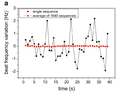
Figure 9: The experimental frequency shift reported in Fig.9(a) of ref.[47] (courtesy Optics Communications). The black dots give the instantaneous signal, the red dots give the signal averaged over 1640 sequences. For a laser frequency $\nu_{0}=2.82\cdot 10^{14}$ Hz a $\Delta\nu=\pm 1$ Hz corresponds to a fractional value $\Delta\nu/\nu_{0}$ of about $\pm 3.5\cdot 10^{-15}$.

After having obtained these first indications, we have tried to understand the meaning of this irregular signal. Namely is it just spurious noise (e.g. thermal noise [77]) or could it represent a genuine signal? As a check, we have then compared with other two experiments, ref.[46] and ref.[50], where the optical cavities were made of different materials and were operating at a cryogenic temperature. Again the same $10^{-15}$ level. Since it is extremely unlike that spurious effects remain the same for experiments operating in so different conditions, it is natural to explore the possibility that such $10^{-15}$ signal admits a physical interpretation.

Therefore, applying to the physical vacuum the same model used successfully for the classical experiments, we will tentatively express this observed fractional shift in terms of a cosmic earth velocity and of a refractive index ${\cal N}_{v}$ as

$$\left|{{\Delta\nu(\theta)}\over{\nu_{0}}}\right|_{\rm exp}=\left|{{\Delta\bar{c}_{\theta}}\over{c}}\right|_{\rm exp}\sim({\cal N}_{v}-1)~{}(v^{2}/c^{2})~{}\sim{\cal O}(10^{-15})$$ (62)

For $v\sim$ 300 km/s, this supports our previous idea of a tiny refractivity $\epsilon_{v}=({\cal N}_{v}-1)\sim 10^{-9}$ for the physical vacuum established in an apparatus placed on the earth surface. Therefore, it is now the time to recall the scenario of ref.[52] which could indeed explain such result.

7..2 A $10^{-9}$ refractivity for the vacuum on the earth surface

The idea of a non-zero vacuum refractivity may have different motivations. The perspective of ref.[52] was inspired by the so called emergent gravity approach [78]$-$ [84] where the introduction of a non-trivial metric field $g_{\mu\nu}(x)$ is considered in analogy with the hydrodynamic limit of many condensed-matter systems. This emergent interpretation is made manifest in a parametric dependence of the metric on some auxiliary, inducing-gravity fields $s_{k}(x)$, i.e. $g_{\mu\nu}(x)=g_{\mu\nu}[s_{k}(x)]$. As in the pioneering Yilmaz derivation based on the static Newtonian potential [85, 86], Einstein equations for the metric would then follow from the equations of motion for the $s_{k}$’s in flat space, after introducing a suitable stress tensor for these auxiliary fields. In this way, one could (partially) fill the conceptual gap with classical General Relativity.

An interesting consequence derives from the boundary condition $g_{\mu\nu}[s_{k}=0]=\eta_{\mu\nu}$. In fact, if the $s_{k}$’s are understood as excitations of the physical vacuum, which therefore vanish identically in its equilibrium state, one could easily understand [80] why the energy of the unperturbed vacuum plays no role. This perspective of a non-gravitating vacuum energy [80] provides, perhaps, the most intuitive solution of the so called cosmological-constant problem usually mentioned in connection with the quantum vacuum. In this sense, with this type of approach, one is taking seriously Feynman’s words: “The first thing we should understand is how to formulate gravity so that it doesn’t interact with the vacuum energy” [87].

Another interesting aspect of this approach is that, even without knowing the underlying $s_{k}$’s, in the simplest case of a static metric all dynamical effects are equivalent to two basic ingredients: i) local modifications of the physical clocks and rods and ii) local modifications of the velocity of light. Therefore, with this interpretation of the observed curvature, one could try to test the fundamental assumption of General Relativity that, in the presence of gravity, the velocity of light in vacuum $c_{\gamma}$ is still a universal constant, namely it remains the same, basic parameter $c$ of Lorentz transformations. Notice that, here, we are not considering the so called coordinate-dependent speed of light. Rather, we are focused on the true, physical $c_{\gamma}$ as obtained from experimental measurements in vacuum optical cavities placed on the earth surface. Thus in principle, a precise measurement establishing that $c_{\gamma}\neq c$ could give information on the fundamental mechanisms at the base of the gravitational interaction.

For the various aspects of space-time measurements, a very clear reference is Cook’s article “Physical time and physical space in general relativity” [88]. There, the appropriate units of time and length, respectively $d\tau$ and $dl$, are defined to ensure that all observers measure the same, universal speed of light (“Einstein postulate”). For a static metric, these definitions are $d\tau^{2}=g_{00}dt^{2}$ and $dl^{2}=g_{ij}dx^{i}dx^{j}$. Thus, in General Relativity, the condition $ds^{2}=0$, which governs the propagation of light, can be expressed formally as

$$ds^{2}=c^{2}d\tau^{2}-dl^{2}=0$$ (63)

and, by construction, gives always the same speed $dl/d\tau=c$.

But, if the physical units were instead $d\hat{\tau}$ and $d\hat{l}$ with, say, $d\tau=q~{}d\hat{\tau}$ and $dl=p~{}d\hat{l}$, the same condition

$$ds^{2}=c^{2}q^{2}d\hat{\tau}^{2}-p^{2}d\hat{l}^{2}=0$$ (64)

would now be interpreted differently as

$$c_{\gamma}={{d\hat{l}}\over{d\hat{\tau}}}=c~{}{{q}\over{p}}\equiv{{c}\over{{\cal N}_{v}}}$$ (65)

The possibility of different units is thus a simple motivation for a vacuum refractive index ${\cal N}_{v}\neq 1$.

To fix the ideas, we will start from the unambiguous point of view of special relativity: the right space-time units are those for which the speed of light in the vacuum $c_{\gamma}$, when measured in an inertial frame, coincides with the basic parameter $c$ of Lorentz transformations. But inertial frames are just an idealization. Therefore the physical realization is to assume standards of distance and time which can change locally but such that the identification $c_{\gamma}=c$ holds in the asymptotic condition which is as close as possible to an inertial frame. This asymptotic condition corresponds to measure $c_{\gamma}$ in a freely falling frame and is crucial for an operational definition of the otherwise unknown quantity $c$.

With this premise, an observer $S^{\prime}$ placed on the earth surface can still describe light propagation in different ways. We address the reader to ref.[52], where these aspects were originally discussed, and to refs.[39, 40] for further refinements. The whole idea, however, is simple and can be reduced to Fig.10. An observer $S^{\prime}$ placed on the earth surface is in free-fall with respect to all masses in the Universe but not with respect to the gravitational field of the earth. Its effect can be schematically represented by means of a heavy mass $M$ carried on board of the elevator.

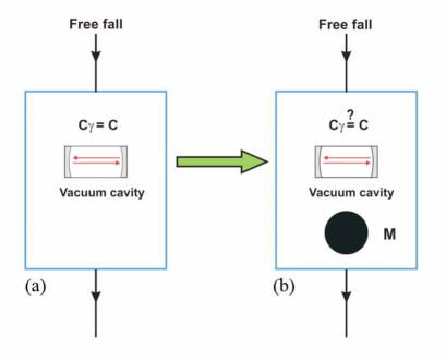
Figure 10: An intuitive visualization of two physically distinct situations. In case (b) a heavy mass $M$ is carried on board of a freely-falling system. Differently from the ideal case (a), the mass $M$ could introduce a vacuum refractivity so that now $c_{\gamma}\neq c$.

The two situations in panels (a) and (b) of Fig.10 are physically distinct but in General Relativity it is assumed that both observers will measure the same $c$ of Lorentz transformations. A non-zero vacuum refractivity, for system (b), can thus be expressed as

$$\epsilon_{v}={\cal N}_{v}-1\sim{{z}\over{2}}~{}\left({{2|\delta U|}\over{c^{2}}}\right)$$ (66)

where $\delta U$ is the extra Newtonian potential produced by the heavy mass $M$ at the experimental setup. In General Relativity one assumes $z=0$ while the two non-zero values ($z=$ 1 or 2) account for the two alternatives traditionally reported in the literature for the effective refractive index in a gravitational potential (see the discussion in refs.[39, 40] and in particular Broekaert’s footnote ³ [89]). In our case, by introducing the Newton constant, the radius $R$ and the mass $M$ of the earth, so that $\delta U={{G_{N}M}\over{R}}$, we find

$$\epsilon_{v}\sim{{z}\over{2}}~{}1.4\cdot 10^{-9}$$ (67)

We emphasize that, regardless of whether $z=$ 1 or 2, the velocity of light in a vacuum cavity on the earth surface, panel (b) in our Fig.10, could differ at the level $10^{-9}$ from that ideal value $c$, operationally defined with the same apparatus in a true freely-falling frame, panel (a) in our Fig.10. As discussed at the end of Sect.6, such $\epsilon_{v}\sim 10^{-9}$ was suggested by the last precise measurements of the velocity of light and, by comparing with Eq.(62), could now provide a physical argument to seriously consider the presently observed $10^{-15}$ fractional frequency shift of two vacuum optical resonators. Let us therefore give a closer look at the present experiments.

7..3 A closer look at experiments and numerical simulation of the signal

Most recent ether-drift experiments measure the frequency shift $\Delta\nu$ of two rotating optical resonators. To this end, let us re-write Eq.(26) as

$${{\Delta\nu(t)}\over{\nu_{0}}}={{\Delta\bar{c}_{\theta}(t)}\over{c}}\sim\epsilon{{v^{2}(t)}\over{c^{2}}}\cos 2(\omega_{\rm rot}t-\theta_{2}(t))$$ (68)

where $\omega_{\rm rot}$ is the rotation frequency of the apparatus. Therefore one finds

$${{\Delta\nu(t)}\over{\nu_{0}}}\sim 2{S}(t)\sin 2\omega_{\rm rot}t+2{C}(t)\cos 2\omega_{\rm rot}t$$ (69)

with $C(t)$ and $S(t)$ given in Eqs.(28) for $\epsilon=\epsilon_{v}$

$$2C(t)=\epsilon_{v}~{}{{v^{2}_{x}(t)-v^{2}_{y}(t)}\over{c^{2}}}~{}~{}~{}~{}~{}~{}~{}2S(t)=\epsilon_{v}~{}{{2v_{x}(t)v_{y}(t)}\over{c^{2}}}$$ (70)

and $v_{x}(t)=v(t)\cos\theta_{2}(t)$, $v_{y}(t)=v(t)\sin\theta_{2}(t)$. For a non rotating apparatus, as in Fig.9, the fractional frequency shift is thus simply $2C(t)$.

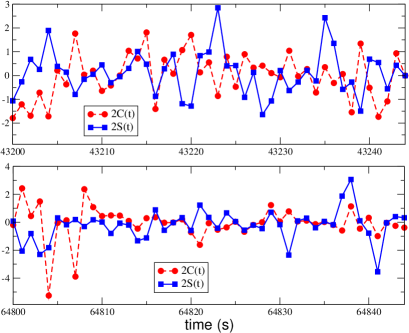
Figure 11: For $\epsilon_{v}$ as in Eq.(67) and $z=2$, we report in units $10^{-15}$ two typical sets of 45 seconds for the two functions $2C(t)$ and $2S(t)$ of Eq.(69). The two sets belong to the same random sequence and refer to two sidereal times that differ by 6 hours. The boundaries of the stochastic velocity components Eqs.(36) and (37) are controlled by $(V,\alpha,\gamma)_{\rm CMB}$ through Eqs.(30) and (40). For a laser frequency of $2.8\cdot 10^{14}$ Hz [51], the range $\pm 3.5\cdot 10^{-15}$ corresponds to a typical frequency shift $\Delta\nu$ in the range $\pm 1$ Hz, as in our Fig.9.

The present analysis of the data is the following. For short-period observations of a few days, the frequency shifts, measured upon rotation of the apparatus, are used to extract the instantaneous 2C(t) and 2S(t) through Eq.(69). These data are then compared with the parameterizations Eqs.(33) and (34) to fit the $C_{k}$ and $S_{k}$ Fourier coefficients. From very extensive observations, the present values of these coefficients are at the level $10^{-18}\div 10^{-19}$, i.e. about 1000 times smaller than the typical $10^{-15}$ instantaneous signal.

By recalling our discussion at the beginning of Sect.5, this is exactly the same strategy traditionally adopted for the fringe shifts in the old experiments and that cannot be maintained with a genuine irregular signal. In fact, within our isotropic model, see Eqs.(4.) and (42)), one would find $\langle C(t)\rangle_{\rm stat}=0$ and $\langle S(t)\rangle_{\rm stat}=0$ at any time $t$ and mean values $(C_{k})^{\rm avg}=0$, $(S_{k})^{\rm avg}=0$ for all Fourier coefficients. Therefore, with an irregular but genuine signal a different type of analysis is needed.

To compare with the data, we have performed numerical simulations in our isotropic stochastic model of Sect.4 with $\epsilon_{v}$ as in Eq.(67). As a first illustration, we show in Fig.11 two sequences of the instantaneous values for 2C(t) and 2S(t). The two sets belong to the same random sequence and refer to two sidereal times that differ by 6 hours. The set $(V,\alpha,\gamma)_{\rm CMB}$ was adopted to control the boundaries of the stochastic velocity components through Eqs.(29), (30) and (40). The value $\phi=52$ degrees was also fixed to reproduce the average latitude of the laboratories in Berlin and Düsseldorf. For a laser frequency of $2.8\cdot 10^{14}$ Hz [51], the interval $\pm 3.5\cdot 10^{-15}$ of these dimensionless amplitudes corresponds to a random instantaneous frequency shift $\Delta\nu$ in the typical range $\pm 1$ Hz, as in our Fig.9.

For a more quantitative analysis we have considered the result of ref.[51] for the average variation of the frequency shift over 1 second, see their Fig.3, bottom part. This corresponds to a Root Square of the Allan Variance (RAV) of about $0.24$ Hz, or $8.5\cdot 10^{-16}$ at a fractional level. In general the RAV describes the time dependence of an arbitrary function $f=f(t)$ which can be sampled over time intervals of length $\tau$. By defining

$${\overline{f}}(t_{i};\tau)={{1}\over{\tau}}\int^{t_{i}+\tau}_{t_{i}}dt~{}f(t)\equiv{\overline{f}}_{i}$$ (71)

one generates a $\tau-$dependent distribution of ${\overline{f}}_{i}$ values. In a large time interval $\Lambda=M\tau$, the RAV is then defined as

$$\sigma_{A}(f,\tau)=\sqrt{\sigma^{2}_{A}(f,\tau)}$$ (72)

where

$$\sigma^{2}_{A}(f,\tau)={{1}\over{2(M-1)}}\sum^{M-1}_{i=1}\left({\overline{f}}_{i}-{\overline{f}}_{i+1}\right)^{2}$$ (73)

The integration time $\tau$ is given in seconds and the factor of 2 is introduced to obtain the same standard variance for uncorrelated data as for a white-noise signal with uniform spectral amplitude at all frequencies.

To understand the characteristics of our signal, we have thus simulated one-day measurements of $2C(t)$ and $2S(t)$ at steps of 1 second. The RAV and the standard variance agree to good accuracy, so that the signal of our isotropic stochastic model could be approximated as a pure white noise. From these simulations of one-day measurements, ($z=$ 1 or 2), we obtained mean values $\langle 2C\rangle_{\rm day}=-1.6\cdot(z/2)\cdot 10^{-18}$, $\langle 2S\rangle_{\rm day}=4.3\cdot(z/2)\cdot 10^{-18}$ and variances

$$\left[\sigma_{A}(2C,1)\right]_{\rm simul}={{z}\over{2}}(8.7\pm 0.8)\cdot 10^{-16}$$ (74)

$$\left[\sigma_{A}(2S,1)\right]_{\rm simul}={{z}\over{2}}(9.6\pm 0.9)\cdot 10^{-16}$$ (75)

Here the $\pm$ uncertainties reflect the observed variations due to the truncation of the Fourier modes in Eqs.(36), (37) and to the dependence on the random sequence. From Eq.(69), by combining quadratically these two sigma’s, we estimate

$$\left[\sigma_{A}({{\Delta\nu}\over{\nu_{0}}},1)\right]_{\rm simul}\sim\sqrt{{{1}\over{2}}~{}\sigma^{2}_{A}[2C,1]_{\rm simul}+{{1}\over{2}}~{}\sigma^{2}_{A}[2S,1]_{\rm simul}}\sim{{z}\over{2}}(9.2\pm 0.9)\cdot 10^{-16}$$ (76)

so that, for a laser frequency $\nu_{0}=2.8\cdot 10^{14}$ Hz [51], we would predict an average RAV

$$\left[\sigma_{A}(\Delta\nu,1)\right]_{\rm simul}\sim{{z}\over{2}}(0.26\pm 0.03)~{}{\rm Hz}$$ (77)

of the frequency shift at 1 second. This estimate should be compared with the mentioned experimental value

$$\left[\sigma_{A}(\Delta\nu,1)\right]_{\rm exp}\sim 0.24~{}{\rm Hz}$$ (78)

reported in ref.[51]. The good agreement with our simulated value indicates that, at least for an integration time of 1 second, the correction to our model should be negligible. Also, the data favor $z=2$, which is the only free parameter of our scheme.

Our model, however, makes another definite prediction: during the day there should be characteristic modulations which reflect the periodic variations of $\tilde{v}(t)$ Eq.(30) in the plane of the interferometer. For $z=2$ and the typical Central-Europe value $\tilde{v}(t)=(250\div 370)$ km/s, taking into account uncertainties in the simulations, from bins of data centered around the various times $t$, the RAV at 1 second explores the range

$$5\cdot 10^{-16}\lesssim~{}\left[\sigma_{A}({{\Delta\nu}\over{\nu_{0}}},1)\right]_{t}~{}\lesssim 12\cdot 10^{-16}$$ (79)

This range is obtained with our numerical simulation but can be approximated as

$$\left[\sigma_{A}({{\Delta\nu}\over{\nu_{0}}},1)\right]_{t}\sim~{}8.4\cdot 10^{-16}\left({{\tilde{v}(t)}\over{315~{}{\rm km/s}}}\right)^{2}$$ (80)

where $\tilde{v}(t)$ is defined in Eq.(30).

Detecting these periodic variations would therefore give the cleanest test of our picture, provided these variations are not obscured by spurious effects. The simplest strategy for a comparison is to determine, from the spectral amplitude of the experimental signal, the frequency $\omega_{0}$ beyond which the spectral amplitude $\sqrt{S(\omega)}$ becomes flat. Thus, by defining $\tau_{0}\sim\omega_{0}^{-1}$, for integration times $\tau\lesssim\tau_{0}$ the RAV is dominated by the pure white-noise component of the signal. Then, since typically $\tau_{0}\sim$ 1 second, by measuring the experimental RAV at $\tau_{0}$, in different hours of the day, one can directly compare with Eq.(79) .

For a more refined comparison, one could try to generate a colored signal which, as in the real experimental situation, contains various branches (white-noise, pink-noise, random-walk…), and estimate directly the modifications of our basic white-noise component at the various $\tau$’s. Since these modifications depend on the particular experiment, we have decided to consider ref.[25]. This is a high-precision cryogenic experiment, with microwaves of 12.97 GHz, where almost all electromagnetic energy propagates in a medium, sapphire, with refractive index of about 3 (at microwave frequencies). Therefore, an analysis of this experiment will also check our Eq.(61) implying that a fundamental $10^{-15}$ vacuum signal as in (57), with very precise measurements, should also show up in a solid dielectric.

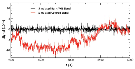
Figure 12: We report two typical sets of 2000 seconds for our basic white-noise (WN) signal and its colored version obtained by Fourier transforming the spectral amplitude of ref.[25].

From Figure 3(c) of [25], the spectral amplitude of this particular apparatus is seen to become flat at frequencies $\omega\geq 0.5$ Hz indicating the order of magnitude estimate $\tau_{0}\sim$ 1 second. In collaboration with Dr. Giancarlo Cella of the VIRGO Collaboration, these data for the spectral amplitude were then fitted to an analytic, power-law form to describe the lower-frequency part 0.001 Hz $\leq\omega\leq 0.5$ Hz. This fitted spectrum was then used to generate a signal by Fourier transform. Finally, very long sequences of this signal were stored to produce “colored” version of our basic white-noise signal. The details of this analysis will be published elsewhere [90].

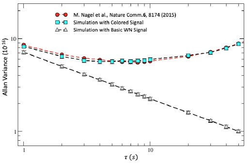
Figure 13: We report the Allan variance for the fractional frequency shift obtained from simulations of sequences of 2000 seconds for our basic white-noise (WN) signal and for its colored version obtained by Fourier transforming the spectral amplitude of ref.[25]. The direct experimental results of ref.[25], for the non-rotating setup, are also shown.

Here we will limit ourselves to report the results of a first set of simulations in intervals of 2000 seconds. To get a qualitative impression of the effect, we report in Fig.12 a sequence of our basic white-noise signal and a sequence of its colored version. By averaging over many 2000-second sequences of this type, the corresponding RAV’s for the two signals are reported in Fig.13. The experimental RAV extracted from Figure 3(b) of ref.[25] is also reported (for the non-rotating setup). At this stage, the agreement of our simulated, colored signal with the experimental data remains satisfactory only up $\tau=$ 50 seconds. Reproducing the signal at larger $\tau$’s will require further efforts but this is not relevant here, our scope being just to understand the modifications of our stochastic signal near the 1-second scale.

From Fig.13 we find that, at the value of interest $\tau=$ 1 second, our predicted white-noise signal $(7.1\pm 0.3)\cdot 10^{-16}$ is changed respectively by about $+15\%$, when comparing with our simulated colored value $(8.2\pm 0.3)\cdot 10^{-16}$, or by about $+20\%$, when comparing with the experimental value of about $8.5\cdot 10^{-16}$. Thus periodic variations of a factor of 2 as in Eq.(79), if present in the experimental data, should remain visible, at least with a systematics at the level of ref.[25].

At the same time, this $8.5\cdot 10^{-16}$, obtained in ref.[25] for the experimental RAV at 1 second, is the same $8.5\cdot 10^{-16}$ that we extracted from the value $\sigma_{A}(\Delta\nu,1)_{\rm exp}\sim$ 0.24 Hz of ref.[51] after normalizing to the laser frequency $\nu_{0}=2.8\cdot 10^{14}$ Hz. Therefore this beautiful agreement, between ref.[51] (a vacuum experiment at room temperature) and ref.[25] (a cryogenic experiment in a solid dielectric), while confirming our predictions Eqs. (57) (61) of a fundamental $10^{-15}$ signal, indicates that periodic variations as in Eq.(79) should also remain visible with the apparatus of ref.[51].

8. Summary and conclusions

Due to the present interpretation of the dominant dipole anisotropy of the Cosmic Microwave Background as a Doppler effect, one may wonder about the reference system where this dipole vanishes exactly. Since the observed motion is, to good approximation, the combination of peculiar motions and reflects local inhomogeneities, one could naturally consider the idea of a global frame of rest, associated with the Universe as a whole, which could characterize the form of relativity physically realized in nature. The isotropy of the CMB could then just indicate the existence of this fundamental system $\Sigma$ that we could conventionally decide to call “ether” but the cosmic radiation itself would not coincide with this type of ether. Due to the fundamental group properties of Lorentz transformations, two observers, individually moving with respect to $\Sigma$, would still be connected by the standard relativistic composition rule of velocities. But ultimate implications could be far reaching. Just think about the interpretation of non-locality in the quantum theory.

Since the answer cannot be found on a pure theoretical ground, physical interpretation is traditionally postponed to the detection of some dragging of light in the earth frame. Namely, to measuring a small angular dependence ${{\Delta\bar{c}_{\theta}}\over{c}}$ of the two-way velocity of light in laboratory and trying to correlate the measurements with the direct CMB observations with satellites in space. The present view is that no such meaningful correlation has ever been observed, all data collected so far (from Michelson-Morley to the modern experiments with optical resonators) being just considered typical instrumental effects in measurements with better and better systematics.

However, if the velocity of light in the interferometers is not the same parameter “c” of Lorentz transformations, nothing would prevent a non-zero dragging. For instance, in experiments in gaseous media with refractive index ${\cal N}=1+\epsilon$, the small fraction of refracted light could keep track of the velocity of matter with respect to the hypothetical $\Sigma$ and produce a direction-dependent refractive index. Then, from symmetry arguments valid in the $\epsilon\to 0$ limit, one would expect ${{|\Delta\bar{c}_{\theta}|}\over{c}}\sim\epsilon(v^{2}/c^{2})$ which is much smaller than the classical expectation ${{|\Delta\bar{c}_{\theta}|_{\rm class}}\over{c}}\sim(v^{2}/2c^{2})$. For $v\sim$ 300 km/s, and inserting the appropriate refractive index, i.e. $\epsilon\sim 2.8\cdot 10^{-4}$ for air and $\epsilon\sim 3.3\cdot 10^{-5}$ for gaseous helium, this reproduces the observed order of magnitude, respectively ${{|\Delta\bar{c}_{\theta}|}\over{c}}\sim 10^{-10}$ and ${{|\Delta\bar{c}_{\theta}|}\over{c}}\sim 10^{-11}$.

In addition, besides being much smaller than classically expected, observable effects could have an irregular nature. This means that the projection of the global velocity field at the site of the experiment, say $\tilde{v}_{\mu}(t)$, could differ non trivially from the local field $v_{\mu}(t)$ which determines the instantaneous direction and magnitude of the drift in the plane of the interferometer. As a definite model, to relate $v_{\mu}(t)$ and $\tilde{v}_{\mu}(t)$, on the basis of some theoretical arguments, we have followed the physical analogy with a turbulent fluid, in particular, with that form of turbulence which, at small scales, becomes statistically homogeneous and isotropic. To this end, the local $v_{\mu}(t)$ was expanded in a large number of Fourier components varying randomly within boundaries which depend on the smooth $\tilde{v}_{\mu}(t)$ determined by the average motion of the earth. In this model, at the small scale of the experiment, statistical averages of vector quantities vanish identically. Therefore, one should analyze the data for ${{\Delta\bar{c}_{\theta}(t)}\over{c}}$ in phase $\theta_{2}(t)$ and amplitude $A_{2}(t)$, which give respectively the direction and magnitude of the local drift, and concentrate on the latter which, being positive definite, remains non-zero under any averaging procedure. Then, even discarding $\theta_{2}(t)$, the time modulations of the statistical average $\langle A_{2}(t)\rangle_{\rm stat}$ could still be used to correlate a genuine signal with the corresponding cosmic motion.

As a proof, we report some remarkable correlations found in the old experiments:

a) by fitting with Eqs.(29) and (30) the smooth polynomial interpolation of the irregular Joos 2nd-harmonic amplitudes in our Fig.7, one finds [37] a right ascension $\alpha({\rm fit-Joos})=(168\pm 30)$ degrees and an angular declination $\gamma({\rm fit-Joos})=(-13\pm 14)$ degrees which are well consistent with the present values $\alpha({\rm CMB})\sim$ 168 degrees and $\gamma({\rm CMB})\sim-$7 degrees.

b) by inspection of our Table 2, if we compare with our Eq.(46), all experiments with light propagating in air give $\tilde{v}_{\rm air}\sim 418\pm 62$ km/s and the two experiments in gaseous helium $\tilde{v}_{\rm helium}\sim 323\pm 70$ km/s. Thus the global average $\langle\tilde{v}\rangle\sim 376\pm 46$ km/s agrees well with the 370 km/s from the direct CMB observations.

c) from the two most precise experiments in Table 2, Piccard-Stahel (Brussels and Mt. Rigi in Switzerland) and Joos (Jena), we find two determinations, $\tilde{v}=360^{+85}_{-110}$ km/s and $\tilde{v}=305^{+85}_{-100}$ km/s respectively, whose average $\langle\tilde{v}\rangle\sim 332^{+60}_{-80}$ km/s reproduces to high accuracy the projection of the CMB velocity at a typical Central-Europe latitude.

Still the simple relation ${{|\Delta\bar{c}_{\theta}(t)|}\over{c}}\sim\epsilon(v^{2}(t)/c^{2})$, while providing a consistent description, does not explain how the earth motion produces the observed small anisotropy in the gaseous systems. Here, in this summary, rather than re-proposing immediately our reasoning of Sect.6, we shall follow the other way round. We will thus first summarize the analysis of Sect.7, for the present experiments in vacuum and in solid dielectrics, and at the very end, armed with these results, return to the mechanism at work in the gaseous media.

In Sect.7, we started from the modern experiments which measure the frequency shift $\Delta\nu(t)$ of two vacuum optical resonators. By considering the most precise experiments, with optical cavities made of different materials, and operating at room temperature and in the cryogenic regime, one gets the idea of a universal, irregular signal with typical fractional magnitude ${{|\Delta\nu(t)|}\over{\nu_{0}}}\sim 10^{-15}$. Within the same model adopted for the classical experiments, we have thus explored the possibility to interpret this signal in terms of a vacuum refractivity $\epsilon_{v}={\cal N}_{v}-1\sim 10^{-9}$ in order to obtain ${{|\Delta\nu(t)|}\over{\nu_{0}}}\sim\epsilon_{v}(v(t)/c)^{2}\sim 10^{-15}$ for the typical $v(t)\sim$ 300 km/s.

This $10^{-9}$ vacuum refractivity could have a precise physical interpretation. In fact, the value $\epsilon_{v}\sim(2G_{N}M/c^{2}R)\sim 1.4\cdot 10^{-9}$ was suggested [52] as a possible signature to distinguish an apparatus on the earth surface from the same apparatus placed in that ideal freely-falling frame which defines the parameter $c$ of Lorentz transformations, see Fig.10. In addition, in our stochastic model, a definite $10^{-15}$ instantaneous signal will coexist with vanishing statistical averages for all vector quantities, such as the $C_{k}$ and $S_{k}$ Fourier coefficients extracted from a standard temporal fit to the data with Eqs.(33) and (34). Our physical model, would thus be immediately consistent with the present $10^{-18}\div 10^{-19}$ limits obtained for these coefficients after averaging over many observations.

Since our signal can be approximated as a universal form of white noise and sets an intrinsic limit to the precision of measurements, for a comparison with experiments, we have then considered the characteristics of the signal for that integration time (typically 1 second) where the pure white-noise branch is as small as possible but other types of noise are not yet important. In this case, when comparing with ref.[51], our numerical simulation of the Allan variance for measurements during a whole day, $\sigma_{A}(\Delta\nu,1)_{\rm simul}=0.26\pm 0.03$ Hz is in complete agreement with the experimental result $\sigma_{A}(\Delta\nu,1)_{\rm exp}\sim$ 0.24 Hz.

We have also emphasized that this 0.24 Hz, when normalized to their laser frequency, gives a fractional shift of $8.5\cdot 10^{-16}$ which is precisely the same obtained, at 1 second, in ref.[25], see our Fig.13. Now, ref.[51] is an experiment running with vacuum cavities, at room temperature and with reference frequency $\nu_{0}=2.8\cdot 10^{14}$ Hz. While ref.[25] is a cryogenic experiment, with microwaves of 12.97 GHz, where almost all electromagnetic energy propagates in a medium, sapphire, with refractive index of about 3. It is impossible that this extraordinary agreement can be due to accidental effects. Therefore, our conclusion: there is a fundamental vacuum signal which shows up in vacuum and in solid dielectrics and whose average magnitude is completely consistent with the vacuum refractivity of ref.[52] and the velocity of 370 km/s from the CMB observation with satellites in space.

We also predict periodic, daily variations in the range $(5\div 12)\cdot 10^{-16}$ for a typical Central-Europe latitude. This range was obtained from our numerical simulation but can also be expressed in a simpler way as

$$\left[\sigma_{A}({{\Delta\nu}\over{\nu_{0}}},1)\right]_{t}\sim~{}8.4\cdot 10^{-16}\left({{\tilde{v}(t)}\over{315~{}{\rm km/s}}}\right)^{2}$$ (81)

where $\tilde{v}(t)$ is defined in Eq.(30). Our simulations at the end of Sect.7 indicate that, for integration time of 1 second, our basic signal is modified by about $20\%$. Therefore these periodic variations, if there, should remain visible.

Let us then return to gaseous media. Namely, which could be a physical mechanism that, starting from a fundamental $10^{-15}$ vacuum signal, enhances the effect, respectively up to $10^{-11}$ and $10^{-10}$ in gaseous helium and air, and finally disappears in solid dielectrics, as in the mentioned very precise cryogenic experiment in sapphire, which gives again the same $10^{-15}$ as in vacuum? Our answer to this question, in Sect.6, was based on the traditional interpretation [44, 45] of those old residuals in terms of small temperature difference $\Delta T^{\rm gas}(\theta)$, of a millikelvin or so, in the gas of the two optical arms. We have, however, obtained the same universal value $\Delta T^{\rm gas}(\theta)=0.2\div 0.3$ mK from the various experiments. Therefore those old estimates, besides being slightly too large, were not catching the basic point: different experiments converge toward the same value and, therefore, the thermal effect cannot be due to local temperature conditions but must have a non-local origin. Our interpretation is that the interactions of the gas molecules with the background radiation are so weak that, on average, only less than 1/10 of the $\Delta T^{\rm CMB}(\theta)$ in Eq.(2) is transferred to bring the gas out of equilibrium. Nevertheless, regardless of its precise value, a universal $\Delta T^{\rm gas}(\theta)\lesssim$ 1 mK can help intuition by explaining the quantitative reduction of the effect in the vacuum limit, where $\epsilon_{\rm gas}\to 0$, and the qualitative difference with solid dielectrics where such tiny temperature differences become irrelevant. We have also observed that, after a century from those old experiments, in room-temperature measurements, values $\Delta T\lesssim$ 1 mK are still state of the art for the precision attainable in temperature differences, see e.g.[72, 73, 74].

In conclusion, by considering old and modern experiments, we have found several correlations between optical measurements in laboratory and the kinematical parameters obtained from the direct CMB observations with satellites in space. These correlations are summarized in the three items a), b) and c) listed above and in the successful quantitative description of the RAV measured in refs.[51] and [25] for the relevant region of integration times of about 1 second where the white-noise branch is as small as possible but other experiment-dependent effects are not yet important. Ours is not the only scheme to analyze the experiments but, yet, fulfills the criterion traditionally adopted to indicate a reference system which could play the role of fundamental frame for relativity. We also observe that, for the same region of integration times, our scheme predicts periodic daily variations of the RAV which should be observable. Therefore, for the importance of the issue, we would expect to receive an experimental confirmation or a disproof. If definitely confirmed, one more complementary test should be performed by placing the vacuum (or solid dielectric) optical cavities on board of a satellite, as in the OPTIS proposal [91]. In this ideal free-fall environment, as in panel (a) of our Fig.10, the typical instantaneous frequency shift should be much smaller (by orders of magnitude) than the corresponding $10^{-15}$ value measured with the same interferometers on the earth surface.

Acknowledgments

We thank Giancarlo Cella for useful discussions and his collaboration.

References

- [1] A. A. Penzias and R. W. Wilson, Astrophys. J. 142, 419 (1965).
- [2] R. B. Partridge and D. T. Wilkinson, Phys. Rev. Lett. 18, 557 (1967).
- [3] C. V. Heer, Phys. Rev. 174, 1611 (1968).
- [4] J. C. Mather, Rev. Mod. Phys. 79, 1331 (2007).
- [5] G. F. Smoot, Rev. Mod. Phys. 79, 1349 (2007).
- [6] M. Yoon and D. Huterer, Ap. J. Lett. 813, L18 (2015).
- [7] J. S. Bell, How to teach special relativity, in Speakable and unspeakable in quantum mechanics, Cambridge University Press 1987, pag. 67.
- [8] H. R. Brown, Physical Relativity. Space-time structure from a dynamical perspective, Clarendon Press, Oxford 2005.
- [9] R. de Abreu and V. Guerra, Electr. J. of Theor. Phys. 12, 183 (2015).
- [10] D. Shanahan, Found. of Phys. 44, 349 (2014).
- [11] A. Ungar, Found. of Phys. 30, 331 (2000).
- [12] J. P. Costella et al., Am. J. Phys. 69, 837 (2001).
- [13] K. O’ Donnell and M. Visser, Eur. J. Phys. 32, 1033 (2011).
- [14] L. Hardy, Phys. Rev. Lett. 68 (1992) 2981.
- [15] G. t Hooft, Search of the Ultimate Building Blocks, Cambridge Univ. Press 1997, p.70.
- [16] M. Consoli, P.M. Stevenson, Int. J. Mod. Phys. A 15, 133 (2000).
- [17] M. Consoli and E. Costanzo, Eur. Phys. Journ. C54, 585 (2008) 285.
- [18] M. Consoli and E. Costanzo, Eur. Phys. Journ. C55, 469 (2008).
- [19] M. Consoli, Found. of Phys. 45, 22 (2015).
- [20] V.Rubakov, Phys. Usp. 51, 759 (2008).
- [21] I. Arraut, Europhysics Letters 111, 61001 (2015).
- [22] S. Deser and R. P.Woodard, Phys.Rev.Lett. 99, 111301 (2007).
- [23] M. E. Soussa, R. P.Woodard, Class.Quant.Grav. 20, 2737 (2003).
- [24] S. Nojiri and S.D. Odintsov, Phys. Lett. B 659, 821 (2008).
- [25] M. Nagel et al., Nature Comm.6, 8174 (2015).
- [26] A. A. Michelson and E. W. Morley, Am. J. Sci. 34, 333 (1887).
- [27] D. C. Miller, Rev. Mod. Phys. 5, 203 (1933).
- [28] A. A. Michelson, et al., Ap. J. 68 (1928) p. 341-402.
- [29] K. K. Illingworth, Phys. Rev. 30, 692 (1927).
- [30] R. Tomaschek, Astron. Nachrichten, 219, 301 (1923), English translation.
- [31] A. Piccard and E. Stahel, Journ. de Physique et Le Radium IX (1928) No.2.
- [32] A. A. Michelson, F. G. Pease and F. Pearson, Nature, 123, 88 (1929).
- [33] A. A. Michelson, F. G. Pease and F. Pearson, J. Opt. Soc. Am. 18, 181 (1929).
- [34] F. G. Pease, Publ. of the Astr. Soc. of the Pacific, XLII, 197 (1930).
- [35] G. Joos, Ann. d. Physik 7, 385 (1930).
- [36] M. Consoli and E. Costanzo, Phys. Lett. A 333, 355 (2004).
- [37] M. Consoli, C. Matheson and A. Pluchino, Eur. Phys. J. Plus 128, 71 (2013).
- [38] M. Consoli, A. Pluchino and A. Rapisarda: Europhysics Lett. 113, 19001 (2016).
- [39] M. Consoli and A. Pluchino, Eur. Phys. Jour. Plus 133, 295 (2018).
- [40] M. Consoli and A. Pluchino, Michelson-Morley Experiments: an Enigma for Physics and the History of Science, World Scientific 2019, ISBN 978-981-3278-18-9.
- [41] M. Consoli, A. Pluchino and A. Rapisarda, Chaos, Solitons and Fractals 44, 1089 (2011).
- [42] M. Consoli, A. Pluchino, A. Rapisarda and S. Tudisco, Physica A394, 61 (2014).
- [43] J. Shamir and R. Fox, N. Cim. 62B, 258 (1969).
- [44] G. Joos, Phys. Rev. 45, 114 (1934).
- [45] R. S. Shankland et al., Rev. Mod. Phys.27, 167 (1955).
- [46] H. Müller, et al. , Phys. Rev. Lett. 91, 020401 (2003).
- [47] Ch. Eisele et al., Opt. Comm. 281, 1189 (2008).
- [48] S. Herrmann, et al., Phys.Rev. D 80, 10511 (2009).
- [49] Ch. Eisele, A. Newsky and S. Schiller, Phys. Rev. Lett. 103, 090401 (2009).
- [50] M. Nagel et al., Ultra-stable Cryogenic Optical Resonators For Tests Of Fundamental Physics, arXiv:1308.5582[physics.optics].
- [51] Q. Chen, E. Magoulakis, and S. Schiller,Phys. Rev. D 93 , 022003 (2016).
- [52] M. Consoli and L. Pappalardo, Gen. Rel. and Grav. 42, 2585 (2010).
- [53] R. V. Pound, Rev. Sci. Instrum. 17, 490 (1946).
- [54] R. W. P. Drever et al., Appl. Phys. B 31, 97 (1983).
- [55] E. D. Black, Am. J. Phys. 69, 79 (2001).
- [56] V. Guerra and R. de Abreu, Eur. J. of Phys. 26, S117 (2005).
- [57] J. C. Maxwell, Ether, Encyclopaedia Britannica, 9th Edition, 1878.
- [58] U. Leonhardt and P. Piwnicki, Phys. Rev. A60, 4301 (1999).
- [59] J. M. Jauch and K. M. Watson, Phys. Rev. 74, 950 (1948).
- [60] R. J. Kennedy, Phys. Rev. 47, 965 (1935).
- [61] R. P. Feynman, R. B. Leighton and M. Sands, The Feynman Lectures on Physics, Addison Wesley Publ. Co. 1963.
- [62] L. Onsager, Nuovo Cimento, Suppl. 6, 279 (1949).
- [63] G. L. Eyink and K. R. Sreenivasan Rev. Mod. Phys. 78, 87 (2006).
- [64] J. J. Nassau and P. M. Morse, Ap. J. 65, 73 (1927).
- [65] L. D. Landau and E. M. Lifshitz, Fluid Mechanics, Pergamon Press 1959, Chapt. III.
- [66] J. C. H. Fung et al., J. Fluid Mech. 236, 281 (1992).
- [67] D. C. Miller, Phys. Rev. 45 (1934) 114.
- [68] L. S. Swenson Jr., the Ethereal Aether, A History of the Michelson-Morley-Miller Aether-Drift Experiments, 1880-1930. University of Texas Press, Austin 1972.
- [69] Loyd S. Swenson Jr., Journ. for the History of Astronomy, 1, 56 (1970).
- [70] J. A. Stone and A. Stejskal, Metrologia 41, 189 (2004).
- [71] T. S. Jaseja, et al., Phys. Rev. 133, A1221 (1964).
- [72] E. R. Farkas and W. W. Webb, Rev. Scient. Instr. 81, 093704 (2010).
- [73] Y. Zhaoa, D. L. Trumperb, R. K. Heilmann, M. L. Schattenburg, Precision Engin. 34, 164 (2010).
- [74] I. P. Prikhodko, A. A. Trusov, A. M. Shkel, Sensors and Actuators A 201, 517 (2013).
- [75] D. A. Jennings et al. , Journ. of Res. Nat. Bur. Stand. 92, 11 (1987).
- [76] A. Brillet and J. L. Hall, Phys. Rev. Lett. 42, 549 (1979).
- [77] K. Numata, A, Kemery and J. Camp, Phys. Rev. Lett. 93, 250602 (2004).
- [78] C. Barcelo, S. Liberati and M. Visser, Class. Quantum Grav. 18, 3595 (2001).
- [79] M. Visser, C. Barcelo and S. Liberati, Gen. Rel. Grav. 34, 1719 (2002).
- [80] G. E. Volovik, Phys. Rep. 351, 195 (2001).
- [81] R. Schützhold, Class. Quantum Gravity 25, 114027 (2008).
- [82] M. Consoli, Class. Quantum Grav. 26, 225008 (2009).
- [83] G. Jannes and G. E. Volovik, JETP Lett.96, 215 (2012).
- [84] S. Finazzi, S. Liberati and L. Sindoni, Phys. Rev. Lett. 108, 071101 (2012).
- [85] H. Yilmaz, Phys. Rev. 111, 1417 (1958).
- [86] B. O. J. Tupper, N. Cimento 19B, 1974 (135); Lett. N. Cimento 14, 627 (1974).
- [87] R. P. Feynman, in Superstrings: A Theory of Everything ?, P. C. W. Davies and J. Brown Eds., Cambridge University Press, 1997, pag. 201.
- [88] R. J. Cook, Am. J. Phys. 72, 214 (2004).
- [89] J. Broekaert, Found. of Phys. 38, 409 (2008).
- [90] G. Cella, M. Consoli and A. Pluchino, in preparation.
- [91] C. Lämmerzahl et al., Class. Quantum Gravity 18, 2499 (2001).