Quantitative Verification with Adaptive Uncertainty Reduction

Abstract

Stochastic models are widely used to verify whether systems satisfy their reliability, performance and other nonfunctional requirements. However, the validity of the verification depends on how accurately the parameters of these models can be estimated using data from component unit testing, monitoring, system logs, etc. When insufficient data are available, the models are affected by epistemic parametric uncertainty, the verification results are inaccurate, and any engineering decisions based on them may be invalid. To address these problems, we introduce VERACITY, a tool-supported iterative approach for the efficient and accurate verification of nonfunctional requirements under epistemic parameter uncertainty. VERACITY integrates confidence-interval quantitative verification with a new adaptive uncertainty reduction heuristic that collects additional data about the parameters of the verified model by unit-testing specific system components over a series of verification iterations. VERACITY supports the quantitative verification of Markov chains, deciding which components are to be tested in each iteration based on factors that include the sensitivity of the model to variations in the parameters of different components, and the overheads (e.g., time or cost) of unit-testing each of these components. We show the effectiveness and efficiency of VERACITY by using it for the verification of the nonfunctional requirements of a tele-assistance service-based system and an online shopping web application.

1 Introduction

Many software systems must satisfy dependability, performance, cost and other requirements not directly related to the functionality they provide. These requirements are termed nonfunctional requirements [3, 4], and their verification needs to consider the stochastic nature of software characteristics such as inputs, workloads, timeouts and failures. As such, stochastic models ranging from Markov chains [5, 6] and probabilistic automata [7, 8] to stochastic Petri nets [9, 10] are widely used to perform this verification. However, ensuring that stochastic models are sufficiently accurate to support this verification is very challenging. While the structure of the models can be extracted from the actual code [11] or from software artefacts such as activity diagrams [6, 12], their parameters (e.g., probabilities, timing and other quantitative information) are affected by uncertainty.

These parameters need to be estimated using data obtained, for instance, from testing the system components individually, or (for systems already in use) from system logs. Point estimators such as the mean of the observed parameter values are typically used for this purpose. However, the point estimation of the uncertain model parameters produces imprecise verification results, and risks causing invalid engineering decisions [13, 14], especially when only few observations are available. In mature subjects like medicine [15, 16] and in established engineering disciplines like civil [17] and mechanical [18] engineering, this risk is deemed unacceptable, and it is mitigated by computing confidence intervals for the model parameters and the verified properties [19, 20]. In contrast, this risk is rarely considered in software performance and dependability engineering. Instead, the research in this area focuses on devising new techniques, tools and applications for the verification of stochastic models, under the strong assumption that using point estimates for the model parameters is sufficiently accurate.

To address the risk of invalid decisions associated with this assumption, we introduce VERACITY, a tool-supported approach for the quantitative verification of Markov chains under epistemic parametric uncertainty. Uncertainty is termed epistemic when it is due to insufficient data (and therefore reducible by gathering additional data), and aleatory when it is intrinsic to the analysed system (and therefore irreducible) [21].

VERACITY builds on our previous research on computing confidence intervals for the reliability, performance and other nonfunctional properties of a system [13, 22]. This computation uses a parametric Markov chain (i.e., a Markov chain with unknown state transition probabilities) that models the system behaviour, and observations of the system behaviour available from component unit testing, runtime monitoring or system logs. However, when insufficient observations are available, these confidence intervals are too wide to verify whether nonfunctional requirements that impose constraints on such properties are satisfied. As an example, given too few observations, the $99\%$ confidence interval for the probability that user requests are handled successfully by a web server may be $[0.76,0.98]$, which is too wide for verifying the requirement ‘The web server shall handle user requests with a success probability of at least 0.92 at 99% confidence level.’ To handle this frequently encountered problem efficiently, VERACITY obtains additional observations by unit-testing specific system components over a series of adaptive uncertainty reduction iterations. The components tested in each iteration are decided using a heuristic that takes into account multiple factors. These factors are detailed later in the paper, and include the sensitivity of the nonfunctional properties to variations in the parameters associated with different components, and the overheads (e.g., time or cost) of testing each of these components.

VERACITY supports both the verification of new system designs, and the verification of planned updates to existing systems. Using VERACITY to decide whether a new system should be deployed or not involves applying our approach with few or no initial observations of the system parameters. Multiple uncertainty reduction iterations are typically required to acquire sufficient observations of the parameters of the system and to reach a decision in this case. In contrast, when deciding whether updated versions of specific system components should be adopted, VERACITY can exploit a large number of initial observations of the parameters associated with the components not being updated. Accordingly, fewer uncertainty reduction iterations are typically necessary in this case, primarily to acquire observations of the parameters associated with the updated components.

[23]

The contributions of the paper are threefold. First, we introduce a new heuristic for the efficient reduction of epistemic parametric uncertainty of Markov chains used in dependability and performance software engineering. Second, we present a new approach that integrates this heuristic with a recently proposed method for formal verification with confidence intervals [13, 22], and a tool that implements the approach, automating the verification of nonfunctional requirements under parametric uncertainty. Finally, we present extensive experimental results showing: (i) the effectiveness of the VERACITY verification approach during initial software development and software updating; and (ii) the efficiency of the VERACITY uncertainty reduction compared to uncertainty reduction by uniformly testing all the components of the system under verification (SUV).

We organised the remainder of the paper as follows. Section 2 defines the probabilistic model checking and formal verification with confidence concepts and notation required to present VERACITY. Section 3 introduces a motivating example that we then use to present our quantitative verification approach in Section 4. Sections 5 and 6 describe the tool support we implemented for our approach, and the case studies we carried out to evaluate VERACITY, respectively. Finally, we discuss related work in Section 7, and we conclude with a brief summary and we suggest directions for future work in Section 8.

2 Preliminaries

2.1 Parametric Markov chains

Definition 1.

A discrete-time Markov chain is a tuple

$$M=(S,s_{0},\mathbf{P},L),$$ (1)

where: $S$ is a finite set of states; $s_{0}\!\in\!S$ is the initial state; $\mathbf{P}:S\!\times\!S\rightarrow[0,1]$ is a transition probability matrix such that, for any states $s,s^{\prime}\!\in\!S$, $\mathbf{P}(s,s^{\prime})$ is the probability of transition from $s$ to $s^{\prime}$ and, for any $s\!\in\!S$, $\sum_{s^{\prime}\in S}\mathbf{P}(s,s^{\prime})\!=\!1$; and $L:S\rightarrow 2^{\mathit{AP}}$ is a function that maps every state $s\!\in\!S$ to those elements of an atomic proposition set $\mathit{AP}$ that hold in state $s$.

Definition 2.

A reward structure over a Markov chain $M$ is a pair of functions $(\rho,\iota)$ that map the states and state transitions of $M$ to non-negative quantities called rewards: $\rho:S\rightarrow[0,\infty)$ and $\iota:S\times S\rightarrow[0,\infty)$.

For Markov chains used in software performance and dependability engineering, the states may correspond to different SUV configurations, to different operations being executed, to different outcomes of these executions, etc. In these models, the rewards may specify expected execution times, resource use and other quantitative characteristics of the operations carried out by the SUV. Finally, the continuous variables used to define the unknown transition probabilities and rewards represent parameters of the SUV components.

Definition 3.

A parametric Markov chain is a discrete-time Markov chain state transition probabilities and/or rewards specified as rational functions (i.e., as fractions whose numerators and denominators are polynomial functions, e.g., $1-p$ or $(1-p_{1})/p_{2}$ [24]) over a set of continuous variables [25].

2.2 Probabilistic computation tree logic

To verify the nonfunctional requirements of a system modelled by a parametric Markov chain, these requirements are expressed in rewards-extended [26] probabilistic computation tree logic (PCTL) [27, 28] with the syntax:

$$\begin{array}[]{l}\Phi::=true\,|\,a\,|\,\Phi\wedge\Phi\,|\,\neg\Phi\,|\,\mathcal{P}_{\bowtie p}[\Psi]\\ \Psi::=\mathrm{X}\;\Phi\;|\;\Phi\;\mathrm{U}^{\leq k}\,\Phi\;|\;\Phi\;\mathrm{U}\;\Phi\\ \Theta::=\mathcal{R}_{\bowtie r}[\mathrm{I}^{=k}]\,|\,\mathcal{R}_{\bowtie r}[\mathrm{C}^{\leq k}]\,|\,\mathcal{R}_{\bowtie r}[\mathrm{F}\,\Phi]\,|\,\mathcal{R}_{\bowtie r}[\mathrm{S}]\end{array}$$ (2)

where $\Phi$ is a state formula, $\Psi$ a path formula, $\Theta$ a reward state formula, $k\!\in\!\mathbb{N}$ a timestep bound, $\bowtie\>\in\!\{\mathord{\leq},<,\mathord{\geq},>\}$ a relational operator, $p\in[0,1]$ a probability bound, $r\geq 0$ a reward bound, and $a\!\in\!AP$ an atomic proposition.

The PCTL semantics is defined using a satisfaction relation $\models$. Given a state $s$ of a Markov chain $M$, $s\models\Phi$ means “$\Phi$ holds in state $s$”, and we have: always $s\models true$; $s\models a$ iff $a\in L(s)$; $s\models\neg\Phi$ iff $\neg(s\models\Phi)$; $s\models\Phi_{1}\wedge\Phi_{2}$ iff $s\models\Phi_{1}$ and $s\models\Phi_{2}$; and $s\models\mathcal{P}_{\bowtie p}[\Psi]$ iff the probability $x$ that paths starting at state $s$ (i.e., sequence of states $s_{1}s_{2}s_{3}\ldots$ such that $s_{1}=s$ and $\forall i>0:\mathbf{P}(s_{i},s_{i+1})>0$) satisfy the path property $\Psi$ satisfies $x\bowtie p$. The next formula $\mathrm{X}\;\Phi$ holds for a path if $\Phi$ is satisfied in the next state on the path; the bounded until formula $\Phi_{1}\,\mathrm{U}^{\leq k}\,\Phi_{2}$ holds for a path iff $\Phi_{1}$ holds in the first $i<k$ path states and $\Phi_{2}$ holds in the $(i+1)$-th path state; and the unbounded until formula $\Phi_{1}\,\mathrm{U}\,\Phi_{2}$ removes the bound $k$ from the time-bounded until formula. Finally, the four reward state formulae $\Theta$ from (2) use the reward operator $\mathcal{R}$ to verify whether the expected reward $x$: at timestep $k$; accumulated up to timestep $k$; accumulated to reach a state that satisfies $\Phi$; and at steady state, respectively, satisfies $x\bowtie r$. For a detailed description of the PCTL semantics, see [26, 27, 28].

Additionally, the notation $\mathrm{F}^{\leq k}\>\Phi\equiv\mathsf{true}\>\mathrm{U}^{\leq k}\>\Phi$ and $\mathrm{F}\>\Phi\equiv\mathsf{true}\>\mathrm{U}\>\Phi$ is used when the left-hand side of a bounded until and until formula, respectively, is $\mathit{true}$; and $\mathcal{P}_{\!=?}[\>\cdot\>]$ and $\mathcal{R}_{\!=?}[\>\cdot\>]$ are used to denote the value of the probability and expected reward from a PCTL state and reward state formula, respectively.

2.3 Formal verification with confidence intervals

Formal verification with confidence intervals [13] is a mathematically based technique for the computation of confidence intervals for nonfunctional properties of systems with stochastic behaviour. Given a parametric Markov chain $M=(S,s_{0},\mathbf{P},L)$ that models the behaviour of a SUV, a PCTL formula $\mathcal{P}_{\!=?}[\>\cdot\>]$ or $\mathcal{R}_{\!=?}[\>\cdot\>]$ corresponding to a nonfunctional property of the SUV, and a confidence level $\alpha\in(0,1)$, the technique computes an $\alpha$ confidence interval for the property.

To perform this computation, the technique starts by calculating confidence intervals for the parameters of the Markov chain by using observations of the outgoing transitions from all states with unknown outgoing transition probabilities. Assuming that $Z\subseteq S$ is the subset of these states, the required observations are provided by a function

$$O:Z\times S\rightarrow\mathbb{N}$$ (3)

that maps each pair of states $(z,s)\in Z\times S$ to the number $O(z,s)$ of times the transition from $z$ to $s$ has been observed, within the given observation time. Given such observations, the confidence interval computation is done in three stages. In the first stage, a confidence interval is calculated for each parameter of the Markov chain. In the next stage, parametric model checking is used to obtain a closed-form expression for the nonfunctional property. This expression is a rational function over the SUV parameters, and is a byproduct of the technique exploited by our VERACITY approach. Finally, in the third stage, the parameter confidence intervals and the property expression are used to establish the confidence interval for the nonfunctional property of interest. For a detailed description of the technique and of a model checker that implements it see [13] and [22], respectively.

The number of available observations and the confidence level $\alpha$ used by the technique influence the width of the confidence interval. Thus, few observations and large $\alpha$ values yield wide confidence intervals that may contain the lower/upper bound that a nonfunctional requirement specifies for the property. In this case, verifying whether the requirement is satisfied or not is impossible, and additional observations need to be collected to allow the computation of a narrower confidence interval that does not contain the bound.

3 Motivating example

To motivate our VERACITY approach, we use a tele-assistance service-based system (TAS) introduced in [34]. TAS aims to support a patient suffering from a chronic condition in the comfort of their home by using: (i) a set of vital-sign monitoring sensors mounted on a medical device worn by the patient; and (ii) remote assistance services offered by emergency, medical and pharmacy service providers.

1. Periodically, the patient’s vital signs are measured by the wearable device , and a third-party medical analysis service is invoked to analyse them in conjunction with the patient’s medical record . Depending on the results of this analysis , TAS may confirm that the patient is fine , may invoke a pharmacy service to request the delivery of different medication to the patient’s home , or may invoke an alarm service . The invocation of the alarm service is also triggered when the patient presses a panic button on the wearable device , and results in a medical team being dispatched to provide emergency assistance to the patient. We assume that the operational profile of the system is known (e.g., from previous deployments) and is given by the probabilities annotating the 1

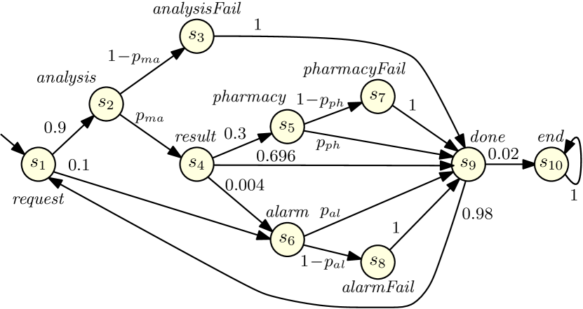
Figure 1: Parametric Markov chain modelling the TAS workflow (adapted from [12])

Table 1: Nonfunctional requirements for the TAS system

ID	Requirement	PCTL formula
R1	The probability that an alarm failure ever occurs during the lifetime of the TAS system shall be below $0.26$.	$\mathcal{P}_{<0.26}[\mathrm{F}\;\mathit{alarmFail}]$
R2	The probability that the handling of a request by the TAS workflow ends with a service failure shall be below $0.04$.	$\mathcal{P}_{<0.04}[\neg\mathit{done}\;\mathrm{U}\;\mathit{serviceFail}]$
R3	The probability that an invocation of the medical analysis service is followed by an alarm failure shall be below $0.0003$.	$\mathcal{P}_{<0.0003}[\neg\mathit{done}\;\mathrm{U}\;\mathit{alarmFail}\{\mathit{analysis}\}]$
[30]

We suppose that a team of software engineers wants to verify whether the third-party services they consider for the implementation of the TAS system satisfy—at 95% confidence level—the nonfunctional requirements from Table 1. We assume that the three services are yet to be tested, and therefore the success probabilities $p_{\mathit{ma}}$, $p_{\mathit{ph}}$ and $p_{\mathit{al}}$ for the medical analysis service, pharmacy service and alarm service, respectively, are unknown . As such, the Markov chain that the engineers can use to verify the TAS requirements is parametric (Figure 1), and the three services must be tested to observe how many of their executions succeed and how many fail (e.g., by not finishing in a timely manner). With these observations, the engineers can use formal verification with confidence intervals (cf. Section 2.3) to compute 95% confidence intervals for the probabilities from the three TAS requirements, which are formally expressed in PCTL in the last column from Table 1. Furthermore, once enough observations are available, these confidence intervals will be sufficiently narrow to ensure that the bounds from the requirements in Table 1 (i.e., $0.26$ for requirement R1, $0.04$ for R2, and $0.0003$ for R3) fall outside the intervals, allowing the engineers to verify whether the requirements are satisfied or not.

However, under the realistic assumption that service invocations take non-negligible time, the engineers will want to complete this verification with as few invocations (i.e., observations) of each service as possible. Minimising this testing effort is particularly important when the verification needs to be performed at runtime, e.g., to find a suitable replacement for a failed component of a system, or when testing a system component has some other cost associated with it (e.g., an invocation charge paid to the provider of a service, or using battery energy on an embedded system). Deciding how many observations to obtain for each service in order to complete the verification of the requirements with minimal testing effort is very challenging. Our VERACITY verification approach addresses this challenge as described in the next section.

4 The VERACITY verification approach

4.1 Problem definition

The VERACITY verification approach is applicable to systems comprising $m>1$ components that can be tested independently. We consider a component-based system whose $n\geq 1$ nonfunctional requirements are of the form

$$\mathit{prop}_{i}\bowtie_{i}\mathit{bound}_{i},$$ (4)

where, for all $i\in\{1,2,\ldots,n\}$, $\mathit{prop}_{i}$ is a nonfunctional system property (e.g., reliability or, through the use of properties that compute the expected reward accumulated to reach states that model the completion of operations, response time), $\bowtie_{i}\>\in\!\{<,\mathord{\leq},\mathord{\geq},>\}$, $\mathit{bound}_{i}\in\mathbb{R}$ places a constraint on the acceptable values of $\mathit{prop}_{i}$, and the $i$-th requirement can be expressed as a PCTL formula $\mathcal{P}_{\bowtie_{i}\mathit{bound}_{i}}[\>\cdot\>]$ or $\mathcal{R}_{\bowtie_{i}\mathit{bound}_{i}}[\>\cdot\>]$ over a parametric Markov chain $M=(S,s_{0},\mathbf{P},L)$. Given such a system, the verification problem addressed by VERACITY is to verify whether the $n$ nonfunctional requirements (4) are satisfied at confidence level $\alpha\in(0,1)$:

1. with minimum overall testing cost;

2. by using a (possibly empty) initial set of observations given by an observation function $O_{0}:Z\times S\rightarrow\mathbb{N}$ with the semantics from (3);

3. by obtaining additional observations through unit-testing the $m$ system components as required, where each unit test of the $j$-th component: (i) generates one additional observation of an outgoing transition for every state in a non-empty set $Z_{j}\subset Z$, such that the state sets $Z_{1}$, $Z_{2}$, …, $Z_{m}$ are disjoint and $\bigcup_{j=1}^{m}Z_{j}=Z$; and (ii) has an associated cost $\mathit{cost}_{j}$, that may represent testing time, resources, price, or a combination thereof.

Using the notation $[l_{i},u_{i}]$ to denote the $\alpha$-confidence interval that can be computed for $\mathit{prop}_{i}$ from (4) after obtaining $n_{1},n_{2},\ldots,n_{m}$ additional observations for component $1,2,\ldots,m$, respectively, the problem addressed by VERACITY is to find $n_{1},n_{2},\ldots,n_{m}\geq 0$ such that the overall testing cost

$$\sum_{j=1}^{m}n_{j}\mathit{cost}_{j}\textrm{ is minimised}$$ (5)

subject to

$$\begin{array}[]{l}\forall i=1..n:(\bowtie_{i}\in\{<,\mathord{\leq}\}\land u_{i}\bowtie_{i}\mathit{bound}_{i})\\ \qquad\qquad\qquad\qquad\lor\;(\bowtie_{i}\in\{>,\mathord{\geq}\}\land l_{i}\bowtie_{i}\mathit{bound}_{i})\end{array}$$ (6)

or

$$\!\!\begin{array}[]{l}\exists i=1..n:(\bowtie_{i}=<\land\>l_{i}\!\geq\!\mathit{bound}_{i})\lor(\bowtie_{i}=\mathord{\leq}\land\>l_{i}\!>\!\mathit{bound}_{i})\\ \qquad\quad\>\lor\;(\bowtie_{i}=>\land\>u_{i}\!\leq\!\mathit{bound}_{i})\lor(\bowtie_{i}=\geq\land\>u_{i}\!<\!\mathit{bound}_{i}).\end{array}$$ (7)

The constraints (6) and (7) correspond to the scenarios where all requirements (4) are satisfied and where at least one of requirements (4) is violated (meaning that the set of requirements as a whole is violated), respectively.

Due to the epistemic uncertainty associated with this verification problem and the stochastic nature of the component-testing results, a minimum overall testing cost We illustrate this limitation with an example. Consider a system that uses two web services, A and B. This system implements a simple workflow: first, it invokes service A, which is available with probability $p_{A}$; next, it invokes service B, which is available with probability $p_{B}$; next, it stops. Suppose that we want to establish whether the probability of successful invocation of both services is at least $0.9$ (i.e., whether $p_{A}p_{B}\geq 0.9$) at confidence level $\alpha=0.95$. If the two unknown probabilities are $p_{A}=0$ (i.e., service A is never available) and $p_{B}=0.95$, then allocating all the testing effort to unit-testing service A is the cheapest strategy for establishing that the requirement is violated, as this strategy will quickly show that $p_{A}$ cannot be large enough for the requirement to be satisfied. Conversely, if $p_{A}=0.95$ and $p_{B}=0$, unit-testing only service B is the cheapest strategy. However, with no prior knowledge about $p_{A}$ and $p_{B}$, it is impossible to always choose the best testing strategy. Therefore, our objective is to achieve an overall testing cost that is, on average, significantly lower than the cost associated with uniformly testing all components. not exceed a predefined testing budget $\mathit{budget}\in\mathbb{N}$.

Example 1.

Consider the TAS system from our motivating example. Its $n=3$ nonfunctional requirements R1–R3 from Table 1 are of the form in (4), are expressed as PCTL formulae over the parametric Markov chain from Figure 1, and need to be verified at confidence level $\alpha=0.95$. The set of Markov chain states with unknown outgoing transition probabilities is $Z=\{s_{2},s_{5},s_{6}\}$, and the (empty) initial set of observations is defined by the function $O_{0}(z,s)=0$ for any $(z,s)\in Z\times S$. The system comprises $m=3$ components that can be tested independently: the medical analysis service (component 1), the pharmacy service (component 2) and the alarm service (component 3). Additionally, invoking one of these services once provides an additional observation of an outgoing transition for the state in one of the disjoint sets $Z_{1}=\{s_{2}\}$, $Z_{2}=\{s_{5}\}$ and $Z_{3}=\{s_{6}\}$, where $Z_{1}\cup Z_{2}\cup Z_{3}=Z$. Finally, to fully cast the task of verifying requirements R1–R3 in the format from our problem definition, we assume that a testing budget $\mathit{budget}\!=\!150000$ is available to complete the verification, and that the per-invocation costs of testing the three services are $\mathit{cost}_{1}\!=\!1$, $\mathit{cost}_{2}\!=\!1$ and $\mathit{cost}_{3}\!=\!2$, e.g., based on the ratios between their mean execution times. We chose a very large budget to ensure that the verification completes without exhausting the budget; this may be unacceptable in practice, in which case the verification might terminate without a decisive result (e.g., if the actual values of some of the $n$ nonfunctional properties are extremely close to their associated bounds).

4.2 VERACITY verification process

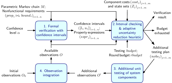
Figure 2: Iterative four-step process of the VERACITY quantitative verification with adaptive uncertainty reduction

To solve the problem from Section 4.1, VERACITY employs the iterative verification process depicted in Figure 2. Each round (i.e., iteration) of this process comprises the four steps described below.

In the first step, formal verification with confidence intervals [13] is used to compute confidence intervals $[l_{1},u_{1}]$, $[l_{2},u_{2}]$, …, $[l_{n},u_{n}]$ at confidence level $\alpha$ and (as a byproduct, as explained in Section 2.3) closed-form expressions $\mathit{expr}_{1}$, $\mathit{expr}_{2}$, …, $\mathit{expr}_{n}$ for the $n$ properties from the nonfunctional requirements (4). The observations $O$ used to compute the $n$ confidence intervals include the initial observations $O_{0}$ and, starting with the second iteration, all the additional observations $O^{\prime}$ obtained in the previous iterations of the process. If the observation set $O_{0}$ is empty, then the confidence interval $[l_{i},u_{i}]$ computed for the $i$-th property in the first iteration is $[0,1]$ or $[0,\infty)$, depending on whether the $i$-th requirement is of the form $\mathcal{P}_{\bowtie_{i}\mathit{bound}_{i}}[\>\cdot\>]$ or $\mathcal{R}_{\bowtie_{i}\mathit{bound}_{i}}[\>\cdot\>]$.

(6)(7), additional observations are needed to complete the verification. Two cases are possible in this situation. First, when the testing $\mathit{budget}$ was fully utilised in the previous VERACITY rounds, the process terminates with an inconclusive ‘budget exhausted’ result. Otherwise, testing budget is still available, and the VERACITY adaptive uncertainty reduction heuristic detailed in Section 4.3 is used to calculate the numbers of additional component observations $\mathit{nobs}_{1}$, $\mathit{nobs}_{2}$, …, $\mathit{nobs}_{m}$ for the next round of the verification process, where

$$\sum_{j=1}^{m}\mathit{nobs}_{j}\mathit{cost}_{j}\approx\mathit{rbudget}$$ (8)

and $\mathit{rbudget}\in[0,\mathit{budget}]$ is a parameter of the VERACITY approach called the round budget. The heuristic is adaptive in the sense that these numbers of additional observations vary from round to round, as the heuristic takes into account the actual observations from all the previous rounds (and any initial observations that may be available). The maximum number of rounds for the verification process is $\lceil\mathit{budget}/\mathit{rbudget}\rceil$. Accordingly, larger round budgets yield fewer rounds, and therefore less opportunity for adaptation but lower overheads (due to the fewer rounds). In contrast, smaller round budgets lead to more rounds, which offer more opportunity for adaptation but also come with higher overheads.

In the third step of the VERACITY process, $\mathit{nobs}_{j}$ tests of component $j$ are carried out for $j=1..m$. As we will explain in Section 5, these tests can be fully automated, or can be performed by a software engineer when requested by the VERACITY verification tool. The results of these tests are then encoded as an observation function $O^{\prime}$ with the format from (3).

Finally, in the fourth and last step of VERACITY, the new observations $O^{\prime}$ are integrated with all the observations obtained in the previous rounds of the process and the initial observations $O_{0}$, and the combined set of all available observations $O$ is used in the next round of the verification process.

Example 2.

For the three requirements for the TAS system from our motivating example, $\bowtie_{1}=\>\bowtie_{2}=\>\bowtie_{3}=<$. Accordingly, the requirements will be verified as satisfied at % confidence level if the observations acquired over successive rounds of the VERACITY verification process (and within the available $\mathit{budget}$) lead to the calculation of % confidence intervals $\left([l_{i},u_{i}]\right)_{i=1..3}$ that satisfy $u_{1}<\mathit{bound}_{1}$, $u_{2}<\mathit{bound}_{2}$ and $u_{3}<\mathit{bound}_{3}$. If, on the other hand, $l_{i}\geq\mathit{bound}_{i}$ for any $i\in\{1,2,3\}$ in one of the verification rounds, the verification process will decide that requirement $i$ is violated at % confidence level, and will terminate in that round. Finally, if the testing $\mathit{budget}$ is used up before sufficient observations of the medical analysis, pharmacy and alarm services are obtained to allow either of these decisions to be made, the verification process will terminate with a ‘budget exhausted’ outcome.

Algorithm 1 Adaptive uncertainty reduction heuristic

1:function NewObs($\mathit{rbudget}$, $M$, $(\mathit{prop}_{i}\!\bowtie_{i}\!\mathit{bound}_{i})_{i=1..n}$, $([l_{i},u_{i}])_{i=1..n}$, $(\!\mathit{expr}_{i})_{i=1..n}$, $(\!\mathit{cost}_{j})_{j=1..m}$, $(Z_{j})_{j=1..m}$, $O$, )

2:    $\mathit{U}=\{i\in 1..n\mid\mathit{bound}_{i}\in[l_{i},u_{i}]\}$ $\triangleright$ desideratum D1

3:    if $\exists i\in\mathit{U}:|\mathit{bound}_{i}\!-\!\textsc{Wrong}(\bowtie_{i},l_{i},u_{i})|/|\mathit{bound}_{i}\!-\!\textsc{Right}(\bowtie_{i},l_{i},u_{i})|<\epsilon_{1}$ then $\triangleright$ desideratum D2

4:       $\mathit{R}\leftarrow\left\{\mathsf{argmin}_{i\in\mathit{U}}|\mathit{bound}_{i}\!-\!\textsc{Wrong}(\bowtie_{i},l_{i},u_{i})|/|\mathit{bound}_{i}\!-\!\textsc{Right}(\bowtie_{i},l_{i},u_{i})|\right\}$

5:    else

6:       $\mathit{R}\leftarrow\mathit{U}$

7:    end if

8:    $\mathit{paramEstimate}\leftarrow\textsc{EstimateParams}(M,O)$

9:    $(\mathit{relevance}_{j}\leftarrow 0)_{j=1..m}$

10:    for $i\in\mathit{R}$ do

11:       $\mathit{weight}=(u_{i}-l_{i})/\max\{|\mathit{bound}_{i}-(l_{i}+u_{i})/2|,\epsilon_{2}\}$ $\triangleright$ desideratum D3

12:       for $j=1$ to $m$ do

13:          $\mathit{sensitivity}\leftarrow\sum_{p\in\textsc{Params}(M,\mathit{Z}_{j})}\left|\frac{\partial\mathit{expr}_{i}(\mathit{paramEstimate})}{\partial p}\right|$ $\triangleright$ desideratum D4

14:          $\mathit{relevance}_{j}\leftarrow\mathit{relevance}_{j}+\mathit{weight}\cdot\mathit{sensitivity}$

15:       end for

16:    end for

17:    for $j=1$ to $m$ do

18:        $\triangleright$ desideratum D5

19:    end for

20:    return $(\mathit{nobs})_{j=1..m}$

21:end function

4.3 Adaptive uncertainty reduction heuristic

4.3.1 Desiderata

Before describing the VERACITY heuristic for partitioning the round testing budget $\mathit{rbudget}$ among the $m$ system components, we present a set of desirable properties (i.e., desiderata) that we propose for any such heuristic:

1. The requirements already verified as satisfied in previous rounds should not influence the partition of the round budget, as the uncertainty associated with these requirements has already been lowered enough to complete their verification.

2. Reaching a resolution on requirements (i.e., on requirements with $\mathit{bound}_{i}\in[l_{i},u_{i}]$) that are likely to be violated should be prioritised when the round budget is partitioned. This desideratum captures the fact that verifying a requirement as violated ends the verification process immediately. Such requirements can be identified by noting that their $\mathit{bound}_{i}$ is very close to the “wrong” end of the confidence interval $[l_{i},u_{i}]$. For instance, if $\mathit{bound}_{i}$ were much closer to $l_{i}$ to $u_{i}$, narrowing down the confidence interval $[l_{i},u_{i}]$ even slightly has a good chance (but is, of course, not certain) of showing that requirement $i$ is violated, and of terminating the verification process.

3. If several requirements influence the partition of $\mathit{rbudget}$, those requirements whose $\mathit{bound}_{i}$ value is closer to the middle of the confidence interval $[l_{i},u_{i}]$ should have a bigger influence. This desideratum reflects the fact that the verification of such requirements is particularly affected by epistemic uncertainty, as a significant narrowing of their confidence intervals is likely to be needed in order to decide whether they are satisfied or violated.

4. The $\mathit{rbudget}$ fraction allocated to each component should reflect the sensitivity of the properties $\mathit{prop}_{1}$ to $\mathit{prop}_{n}$ from (4) to the parameters of that component. For instance, if the closed-form expression for the $i$-th requirement is $\mathit{expr}_{i}=p_{1}+0.01p_{2}$, where $p_{1}$ and $p_{2}$ are probabilities associated with components $C_{1}$ and $C_{2}$, respectively, component $C_{1}$ should be allocated a larger $\mathit{rbudget}$ fraction than $C_{2}$ (all other factors being equal).

5. When the testing of different components is expected to yield similar uncertainty reductions, the round budget partition should prioritise the components with lower testing costs: the value of a new observation of a component is given by the ratio between the (expected) reduction in uncertainty brought by the observation and the cost of that observation.

4.3.2 Algorithm

The numbers of new component observations $\mathit{nobs}_{1}$, $\mathit{nobs}_{2}$, …, $\mathit{nobs}_{m}$ for each VERACITY verification round are computed by function NewObs from Algorithm 1. This function takes the following arguments (cf. Figure 2):

• the round testing budget $\mathit{rbudget}$;

• the Markov chain $M$ and the requirements $(\mathit{prop}_{i}\bowtie_{i}\mathit{bound}_{i})_{i=1..n}$;

• the property confidence intervals $([l_{i},\!u_{i}])_{i=1..n}$ and expressions $(\!\mathit{expr}_{i}\!)_{i=1..n}$ obtained in the previous step of the round;

• the component testing costs $(\mathit{cost}_{j})_{j=1..m}$ and associated state sets with unknown transition probabilities $(Z_{j})_{j=1..m}$;

• the observations $O$ available at the start of the round;

• .

The algorithm has three parts. In the first part (lines 2–7), it identifies the set of relevant requirements $R$ that will influence the partitioning of the round budget. According to desideratum D1, the set $U$ of requirements is computed in line 2. Next, the if statement in lines 3–7 checks if $\mathit{bound}_{i}$ of any requirement is much closer (i.e., $1/\epsilon_{1}$ times closer) to the “wrong” end of the confidence interval $[l_{i},u_{i}]$ than to the “right” end, where:

• the “wrong” end of $[l_{i},u_{i}]$ is the end beyond which requirement $i$ is violated, i.e., $l_{i}$ if $\bowtie_{i}\>\in\!\{<,\mathord{\leq}\}$, and $u_{i}$ otherwise;

• the helper functions Wrong, Right return the respective ends of $[l_{i},u_{i}]$;

• $\epsilon_{1}\!\in\!(0,1)$ is a VERACITY configuration parameter.

As explained in desideratum D2, requirements with this property are likely to be violated. Therefore, if any such requirements exist, only the requirement most likely to be violated is retained in the relevant requirement set $R$ (line 4). Otherwise, $R$ is initialised to include all the requirements (line 6).

The second part of the algorithm (lines 8–16) starts by using the observations $O$ to calculate estimates for each unknown transition probability (i.e., parameter) associated with a state from $Z=\bigcup_{j=1}^{m}Z_{j}$ (line 8). This calculation is performed by the auxiliary function EstimateParams, which estimates the unknown transition probabilities between each state $z\in Z$ and each state $s\in S$ using the observed transition frequency $O(z,s)/\sum_{s^{\prime}\in S}O(z,s^{\prime})$. The special case when $\sum_{s^{\prime}\in S}O(z,s^{\prime})=0$ for one or more states $z\in Z$ may be encountered in the first round, as we allow an empty initial set of observations $O_{0}$ (cf. Section 4.1). In this case, which we do not show in Algorithm 1 in order to keep the pseudocode simple, EstimateParams raises an exception and the round budget is split uniformly between the components whose state sets $Z_{j}$ include states with zero observations.

Next in this part of the algorithm, a component relevance measure $\mathit{relevance}_{j}$ is first initialised in line 9, and then updated with contributions corresponding to the relevant requirements $R$ by the for loop from lines 10–16. Each such contribution is the product of two factors (line 14) that correspond to desiderata D3 and D4, respectively:

• $\mathit{weight}$, a factor calculated as the ratio between the width of the confidence interval $[l_{i},u_{i}]$ and the distance between $\mathit{bound}_{i}$ and the middle of the interval $[l_{i},u_{i}]$ (line 11, where a small VERACITY configuration parameter $0<\epsilon_{2}\ll 1$ is used to prevent a division by zero);

• $\mathit{sensitivity}$, a measure of the sensitivity of expression $\mathit{expr}_{i}$ to the epistemic uncertainty affecting the parameters of component $j$, calculated by summing the absolute value of the partial derivatives of $\mathit{expr}_{i}$ with respect to every parameter of component $j$ (line 13), where the set of all such parameters is provided by the auxiliary function Params, and the partial derivatives are evaluated for the parameter values estimated in line 8.

The third and final part of the algorithm (lines 17–19) decides the number of new observations for each component based on the relevance and testing cost of that component. desideratum D5, the number of new observations for component $j$ is calculated (in line 18) by

To avoid ending with $\mathit{nobs}_{1}=\mathit{nobs}_{2}=$ $\ldots=\mathit{nobs}_{m}=0$, it is sufficient to use a round budget that satisfies the constraint $\mathit{rbudget}\geq\sum_{j=1}^{m}\mathit{cost}_{j}$ because:

$$\begin{array}[]{l}\forall j=1..m:\mathit{nobs}_{j}=0\\ \implies\forall j=1..m:\mathit{rbudget}\cdot\frac{\mathit{relevance}_{j}}{\sum_{k=1}^{m}\mathit{relevance}_{k}}<\mathit{cost}_{j}\\ \implies\sum_{j=1}^{m}\left(\mathit{rbudget}\cdot\frac{\mathit{relevance}_{j}}{\sum_{k=1}^{m}\mathit{relevance}_{k}}\right)<\sum_{j=1}^{m}\mathit{cost}_{j}\\ \implies\mathit{rbudget}<\sum_{j=1}^{m}\mathit{cost}_{j}.\end{array}$$

To achieve good progress with the verification process, $\mathit{rbudget}$ should in fact be much larger (e.g., at least one order the magnitude larger) than $\sum_{j=1}^{m}\mathit{cost}_{j}$ in practice.

For improved readability, a couple of efficiency improvements are not included in Algorithm 1. , the function Params and the partial derivatives required for factor $\mathit{sensitivity}$ (line 13) can be precomputed once (in the first round of the VERACITY verification process), as the SUV parameters associated with a component do not change; only the evaluations of the precomputed partial derivatives need to be done in each round, for the new $\mathit{paramEstimate}$ from that round.

With these improvements in place, the complexity of algorithm is $\mathsf{O}(mn)$, because of the two nested for loops from lines 10–16 and 12–15, respectively. This is typically negligible compared to the complexity of the formal verification with confidence intervals and the additional unit testing from steps one and three of the VERACITY verification process, respectively.

Example 3.

Figure 3 shows the difference between the verification of the TAS nonfunctional requirements from Table 1 using the VERACITY verification process from Figure 2 with: (a) our adaptive uncertainty reduction heuristic from Algorithm 1; and (b) our heuristic replaced with a uniform splitting of the round testing budget among the three system components. These results were obtained assuming that the unknown probabilities from the Markov chain in Figure 1 were $p_{\mathit{al}}=0.94$, $p_{\mathit{ma}}=0.99$ and $p_{\mathit{ph}}=0.95$, and using random number generators to synthesise additional observations $O^{\prime}$ based on these probabilities in the additional unit testing step of the VERACITY verification process from Figure 2. The verification was performed with a round budget $\mathit{rbudget}=5000$, unlimited overall testing $\mathit{budget}$, and the default values $\epsilon_{1}=0.15$ and $\epsilon_{2}=10^{-6}$ for the two parameters of the VERACITY heuristic from Algorithm 1.

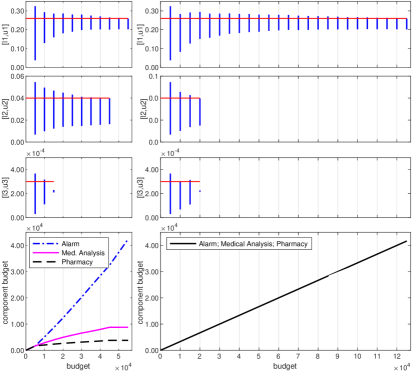
(a) VERACITY                             (b) uniform uncertainty reduction

Figure 3: Verification of the nonfunctional requirements for the TAS system from the motivating example using (a) VERACITY adaptive vs. (b) uniform uncertainty reduction

The top three pairs of graphs from Figure 3 show the 95% confidence intervals $([l_{i},u_{i}])_{i=1..3}$ (depicted as vertical lines) for the nonfunctional properties from the three TAS requirements from Table 1. These confidence intervals become narrower as additional observations are obtained in each round of the verification process, until they are narrow enough to fit completely under the $\mathit{bound}_{i}$ threshold (drawn as a horizontal line) from their associated requirement, i.e., until $u_{i}<\mathit{bound}_{i}$. As soon as this condition is met for a confidence interval $[l_{i},u_{i}]$, that interval is no longer calculated in subsequent verification rounds. When the condition is met for all three confidence intervals, the epistemic uncertainty was reduced sufficiently to conclude that all requirements are satisfied, and the verification process terminates successfully. As shown by these graphs, VERACITY and the uniform uncertainty reduction method finish the verification of each requirement after a different number of verification rounds, and VERACITY completes the verification of the entire set of requirements with an overall testing cost of $55,000$ compared to a 127% higher overall testing cost of $125,000$ for the approach based on uniform uncertainty reduction. We also note in these graphs that the lower bounds of confidence intervals are not always increasing and the upper bounds of confidence intervals are not always decreasing from one VERACITY iteration to the next. As explained in [13]

The bottom pair of graphs from Figure 3 shows the cumulative testing cost per system component. When uniform uncertainty reduction is used, this cost is identical for all components, and is growing linearly with the number of verification rounds. In contrast, for the VERACITY approach, the cumulative cost grows at different rates for different components. Furthermore, the rate of growth for any single component varies across verification rounds because VERACITY continually adapts its partitioning of the round budget to the observations acquired in previous rounds, and to the effect that these observations have on confidence intervals $([l_{i},u_{i}])_{i=1..3}$.

5 Implementation

We implemented the VERACITY verification process as a Java tool built on top of our FACT model checker [22]. The VERACITY tool takes as input: a parametric Markov chain $M$ expressed in the PRISM modelling language [30] and annotated with the component costs $\left(\mathit{cost}_{j}\right)_{j=1..m}$ and state sets $\left(\mathit{Z}_{j}\right)_{j=1..m}$, and with the initial observations $O_{0}$; a set of PCTL-encoded nonfunctional requirements; and a confidence level $\alpha$.

The overall testing $\mathit{budget}$ and round testing budget $\mathit{rbudget}$ are specified via a configuration file. In addition, this configuration file allows the user to optionally specify a component testing script that the tool can execute with the command

$$\texttt{testing-script}\;\>j\;\>nobs_{j}$$

in order to obtain $\mathit{nobs}_{j}$ additional observations for component $j$ automatically in the third step of the VERACITY verification process (cf. Figure 2). If provided, this script needs to run $\mathit{nobs}_{j}$ unit-test against component $j$ (e.g., by invoking the appropriate third-party service for the TAS system from our motivating example), and to return the $\mathit{nobs}_{j}$ observations from these tests as a list of numbers of transitions from the states in $Z_{j}$ to other states of the Markov chain $M$. Alternatively (i.e., if the testing script is not provided), the tool asks the user to supply the required $\mathit{nobs}_{j}$ observations interactively at each round of the verification process.

Our VERACITY tool uses the model checkers FACT [22] and PRISM [30], as well as MATLAB to compute the confidence intervals and property expressions in the first step of its verification process. As such, the tool supports the same fragment of PCTL as FACT, i.e., non-nested PCTL properties $\mathcal{P}_{\!=?}[\>\cdot\>]$ and all types of PCTL reward properties (cf. Section 2.3). The tool is freely available from our project website https://www.cs.york.ac.uk/tasp/VERACITY, together with detailed instructions and all the models, requirement sets, and results from this paper.

6 Evaluation

We evaluated VERACITY by performing an extensive set of experiments aimed at answering the following research questions (RQs).

RQ1

Does VERACITY reduce the testing budget needed to verify a set of nonfunctional requirements compared to the baseline approach that partitions the testing budget of each verification round equally among SUV components?

RQ2

How effective is VERACITY at reducing the testing budget in scenarios where the SUV components have different testing costs?

RQ3

What effect does adjusting the round budget have on the VERACITY testing budget and verification time?

[39, 40, 41, 42]6.26.3

1. [39, 42]

2. [43][40]

3. [39]

To assess the generality of VERACITY, we report experimental results from two case studies in which VERACITY was applied to software systems from different domains. The first case study was based on the TAS system from our motivating example. In the second case study, we applied VERACITY to the verification of an online shopping web application. This system is introduced in Section 6.1, followed by descriptions of the experiments carried out to address the three research questions in Sections 6.2, 6.3 and 6.4, and by a discussion of threats to validity in Section 6.5.

To enable the reproducibility of our results, we have made all the models, properties and data from our experiments available on the VERACITY project website at https://www.cs.york.ac.uk/tasp/VERACITY, which also presents a third case study that uses VERACITY for a model with more complex parametric probability distributions, and a fourth case study that applies VERACITY to a larger, 18-parameter model.

6.1 Online shopping web application

The system we used for the second case study is an online shopping application adapted from [44]. We modelled the shopping process implemented by this application using a parametric Markov chain that comprises a combination of known and unknown transition probabilities. The known transition probabilities correspond to application components that have been in use for a long time, and for which the values of these probabilities can be determined from application logs. In contrast, the unknown transition probabilities correspond to new versions of several components that the online shopping company’s developers have re-implemented and want to evaluate through A/B testing.

A/B testing [45, 46, 47] is a method for testing a new online-application feature, or a new implementation of an existing feature. Frequently used by leading companies like Amazon, Facebook, Google and Microsoft, the method involves splitting the users of a web application into two sets, such that one set of users is given access to a version of the application that includes the new feature (or the new implementation of a feature), while the other set continues to use the standard version of the application. In this way, A/B testing allows companies to evaluate new features and components, and to decide whether they should be included in their online applications or not.

For our case study, we assume that the engineers want to verify whether the nonfunctional requirements from Table 2 would be satisfied if four application components were to be replaced with new variants of those components. Furthermore, we assume that in order to limit the disruption of the user experience that may occur if these requirements are in fact violated, the company wants to perform this verification with as little A/B testing of each of the four new component implementations as possible.

Table 2: Nonfunctional requirements for the online shopping application

ID	Requirement	PCTL formula
R1	The probability that customers complete the shopping process successfully shall be above $\mathit{bound}_{1}$.	$\mathcal{P}_{>\mathit{bound}_{1}}[\mathrm{F}\;\mathit{success}]$
R2	The probability that the authentication component fails shall be below $\mathit{bound}_{2}$.	$\mathcal{P}_{<\mathit{bound}_{2}}[\mathrm{F}\;\mathit{authFail}]$
R3	The average number of uses of new components per shopping session† shall exceed $\mathit{bound}_{3}$.	$\mathcal{R}_{>\mathit{bound}_{3}}[\mathrm{F}\;\mathit{done}]$
†This is a measure of how far the application users progress with the shopping process before giving up or encountering a component failure.

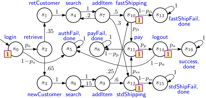
Figure 4: Parametric Markov chain modelling the online shopping application. To enable the verification of requirement R3 from Table 2, the model is augmented with a reward structure that “counts” the uses of new components; this reward structure associates a reward $\rho(s_{0})=\rho(s_{10})=\rho(s_{11})=\rho(s_{12})=\rho(s_{14})=1$ with each state associated with the use of a new component (as shown in small squares next to these states) and zero rewards with the other states and with all state transitions of the Markov chain.

The parametric Markov chain modelling the operation of the online shopping application is shown in Figure 4. In the initial state ($s_{0}$) a customer attempts to login. We assume that the authentication web page is one of the components for which a new implementation needs to be tested, and therefore the probability that the customer can follow the authentication instructions and succeeds to login, denoted $p_{\mathit{a}}$, is unknown. If the authentication succeeds (state $s_{2}$), the customer is identified either as a returning customer (whose settings from the previous shopping session are restored, state $s_{1}$) or as a new customer (for whom default settings are used, state $s_{3}$). In both cases, the customer searches for items to purchase (states $s_{4}$/$s_{6}$) and adds them to the shopping basket (states $s_{7}$/$s_{9}$), until eventually all the required items are in the shopping basket and the customer moves to checkout where they select between two shipping options: fast shipping (state $s_{10}$) or standard shipping (state $s_{12}$). We assume that the probabilities of the incoming transitions into states $s_{1}$, $s_{3}$, $s_{4}$, $s_{6}$, $s_{7}$, $s_{9}$, $s_{10}$ and $s_{12}$ are known (from the previous use of the web application) and have the values from Figure 4.

However, we assume that the web application components for selecting the two shipping options have been re-implemented, and therefore the probabilities $p_{\mathit{fs}}$ and $p_{\mathit{ss}}$ that the customer manages to use them successfully and to reach the payment state $s_{11}$ are unknown. Likewise, we consider that a new version of the payment component has been implemented, and that the probability $p_{p}$ that the customer manages to use it successfully (and to move to the logout state $s_{14}$) is unknown. Finally, we assume that the logout involves the use of the same new authentication component that was used for login, and therefore its (unknown) probability of succeeding is $p_{a}$.

6.2 Research question RQ1

For each of the two systems used in our evaluation, we synthesised and examined a broad range of simulated scenarios (assuming unit component testing costs $\mathit{cost}_{1}=\mathit{cost}_{2}=\ldots=\mathit{cost}_{m}=1$). of the Markov chain $M$ from Figure 2 the bounds from the nonfunctional requirements (4) ensure that the evaluation covered a combination of:

1. scenarios in which all requirements were satisfied: (i) by a narrow margin, i.e., the actual values of the properties from the nonfunctional requirements (4) were close to their associated bounds; (ii) by a wide margin; and (iii) some by a narrow margin and the others by a wide margin;

2. scenarios in which some of the requirements were satisfied and the remaining requirements were violated by: (i) a narrow margin; (ii) a wide margin; and (iii) some by a narrow margin and the others by a wide margin;

3. scenarios in which all requirements were violated by: (i) a narrow margin; (ii) a wide margin; and (iii) some by a narrow margin and the others by a wide margin.

In all the experiments, we used the VERACITY tool in conjunction with a simulated component-testing script with the characteristics described in Section 5. This script emulated the outcome of unit testing the SUV components by using a separate Java pseudorandom number generator for each component. To avoid any bias in the comparison of VERACITY with the baseline approach mentioned in research question RQ1, we used the same pseudorandom number generator seeds in the corresponding experiments for the two approaches.

Case Study 1 (TAS)

For the TAS system, we carried out experiments that examined the effectiveness of VERACITY for a set of 33 scenarios that were randomly generated as described at the beginning of this section. For each of these scenarios, the verification of the TAS nonfunctional requirements was carried out at three confidence levels: $\alpha=0.90$, $\alpha=0.95$ and $\alpha=0.99$. Finally, to answer research question RQ1, two experiments were performed for each scenario and each confidence level $\alpha$: one in which we used the VERACITY uncertainty reduction heuristic, and one in which we used the baseline approach that partitions the testing budget of each verification round equally among the TAS components. In total, we performed 198 verification experiments, corresponding to 33 scenarios $\times$ 3 confidence levels $\times$ 2 uncertainty reduction methods.

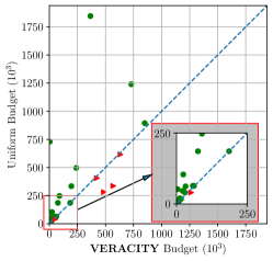
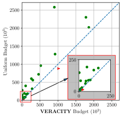
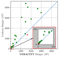
(a) $\alpha=0.90$                                    (b) $\alpha=0.95$                                    (c) $\alpha=0.99$

Figure 5: Testing budgets required to complete the verification of the TAS nonfunctional requirements using the VERACITY and the uniform methods for partitioning the testing round budget among the components of the TAS system. The wide range of budgets required to complete the verification process for different scenarios reflects the variety of these scenarios: in some scenarios, the TAS requirements are satisfied or violated by a wide margin (so less testing is needed, as shown by the inset diagrams), whereas in others some or all of the requirements are satisfied or violated by a narrow margin (so much more testing is needed).

Figure 6: Additional testing budget required to complete the verification of the TAS nonfunctional requirements when the round budget is partitioned using the uniform method instead of the VERACITY method. To ensure readability, the upper part of the boxplots is truncated, meaning that the outliers at 404%, 1200% and 18150% (for $\alpha=0.90$), and at 4252% and 6900% (for $\alpha=0.95$) are not shown. No outliers exist below the bottom whisker of any of the boxplots.

6

6 (Figures 5 and 6).

These results show that VERACITY outperforms the baseline method by completing the verification process with smaller testing budgets for a great majority of the scenarios and at all confidence levels. In a few scenarios, the baseline method performs better than VERACITY (typically only marginally better). This is expected given the stochastic nature of the verified system, and the fact that the verification starts with no knowledge about the behaviour of the three TAS components. Finally, in a small number of additional scenarios, VERACITY achieves only modest testing cost savings. This is also expected, as the best way to reduce epistemic uncertainty in some verification scenarios is to partition the round testing budget approximately equally among the tested system components, and our approach manages to do this well.

The experimental results show that the testing budget reductions enabled by VERACITY are particularly significant when the verification is carried out at higher confidence levels. This is extremely useful for two reasons. First, in real-world scenarios, the nonfunctional requirements of software systems should be verified with high levels of confidence ($\alpha=0.99$ ); deploying a system whose requirements were only verified at a low confidence level introduces significant risks. Second, the testing budget needed to complete the verification increases with the confidence level $\alpha$, as the epistemic uncertainty needs to be reduced much more in order to make decisions with higher confidence. This increase of the required testing budget for larger $\alpha$ values is clearly visible in the scales of the graphs from Figure 5. As such, the scenarios in which VERACITY reduces the cost of testing the most are: (i) of particular practical importance; and (ii) characterised by high testing costs, so the cost reductions achieved by our uncertainty reduction method are especially beneficial.

Case Study 2 (Online shopping web application)

To assess the effectiveness of VERACITY for the online shopping web application (WebApp), we performed a similar suite of experiments to those described for the TAS case study. This time, we examined the ability of VERACITY to reduce testing costs compared to the baseline uncertainty reduction method for the verification of 30 randomly generated scenarios. In each of the 30 scenarios, the verification of the WebApp requirements was carried out at three confidence levels ($\alpha=0.90$, $\alpha=0.95$ and $\alpha=0.99$), for both the VERACITY and the uniform uncertainty reduction methods, giving a total of 180 experiments.

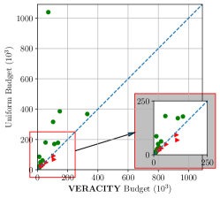
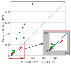
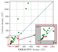
(a) $\alpha=0.90$                                    (b) $\alpha=0.95$                                    (c) $\alpha=0.99$

Figure 7: Testing budgets required to complete the verification of the WebApp nonfunctional requirements using the VERACITY and the uniform methods for partitioning the testing round budget among the components of the online shopping system.

• ;

Figures 7 and 8 summarise the results of these experiments. As for the TAS system, VERACITY successfully reduces the testing budget required to complete the verification of the nonfunctional requirements, across a wide range of testing budget needs (where small testing budgets are needed when the requirements are satisfied or violated by a wide margin, and large budgets when some or all of the requirements are narrowly satisfied/violated). In the small number of scenarios where the uniform round budget partitioning method achieves better results, the overall testing budget is small, and the VERACITY-based verification is typically only marginally more expensive. Again, many significant budget reductions occur when (i) the baseline method budget is high and (ii) the requirements are verified at higher confidence levels. For instance, all of the baseline method budgets above 400,000 from Figure 7 (one for $\alpha=0.90$, four for $\alpha=0.95$, and three for $\alpha=0.99$) are at least halved by VERACITY.

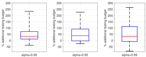
Figure 8: Additional testing budget required to complete the verification of the WebApp nonfunctional requirements when the round budget is partitioned using the uniform method instead of the VERACITY method. To ensure readability, the upper part of the boxplots is truncated at 300%, meaning that the outliers at 616% and 1344% (for $\alpha=0.90$) are not shown. No outliers exist below the bottom whisker of any of the boxplots.

12

6.3 Research question RQ2

6.2 practical situations the costs of testing different components of a system are different. One situation when this is likely to be true is, for instance, when these costs represent the times required for the regression testing of a software system with several modified components [48]. Another situation when this may apply is for testing different web services at runtime, when a limited overall time (i.e., testing budget) is available to verify whether using these services as part of a service-based system like TAS satisfies a set of nonfunctional requirements [5]. This is also likely to be true for the A/B testing of new features of an online application [45, 46, 47] like the shopping application from Section 6.1, where these costs may represent the different (expected) business impact of each of the new features not working as intended.

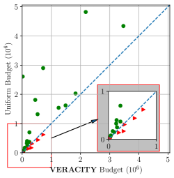
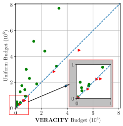
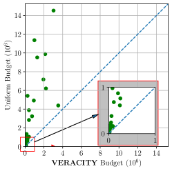
(a) TAS, $\alpha=0.90$                          (b) TAS, $\alpha=0.95$                          (c) TAS, $\alpha=0.99$

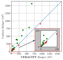
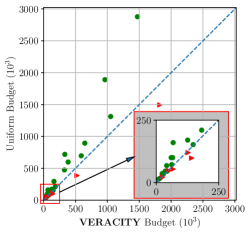
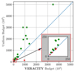
(d) WebApp, $\alpha=0.90$                  (e) WebApp, $\alpha=0.95$                  (f) WebApp, $\alpha=0.99$

Figure 9: Testing budgets required to complete the verification process using the VERACITY and the uniform methods for partitioning the testing round budget among the components of the TAS and WebApp systems.

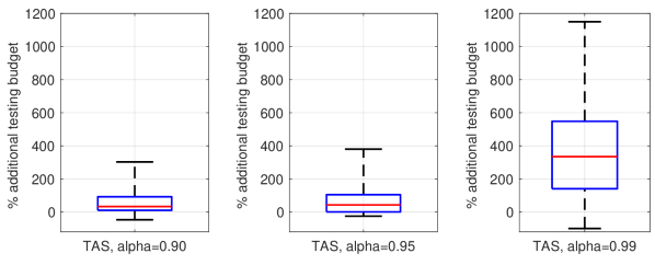
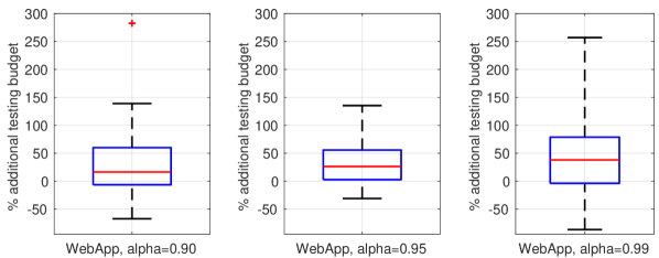
Figure 10: Additional testing budget required to complete the verification of the TAS and WebApp nonfunctional requirements when the round budget is partitioned using the uniform method instead of the VERACITY method. To ensure readability, the upper part of the TAS boxplots is truncated at 1200%, meaning that two TAS outliers at 12950% (for $\alpha=0.90$) and at 1984% (for $\alpha=0.99$) are not shown. No other hidden outliers exist for any of the boxplots.

To evaluate the usefulness of VERACITY in such situations, we repeated all the experiments from Section 6.2 assuming different testing costs for the components of the TAS and WebApp systems from our two case studies. To this end, we took each of the 33 TAS verification scenarios and of the 30 WebApp verification scenarios, and we assigned randomly generated testing costs in the interval $[1,5]$ to the three TAS components and the four WebApp components, respectively.

• ;

• .

The testing budgets required to complete the verification process using the VERACITY and the baseline round-budget partitioning methods in these scenarios with different component testing costs are compared in Figures 9 and 10. As in the scenarios with the same testing costs for all components, our VERACITY verification approach outperforms the baseline verification approach in the majority of the examined scenarios, often by a large margin. As shown in Figure 10, this margin increases as $\alpha$ increases. This increase is particularly significant for the TAS system, where the median additional testing budget required by the baseline verification approach grows from 33% at $\alpha=0.90$ to 42% at $\alpha=0.95$, and 335% at $\alpha=0.99$. This growth is less pronounced but still present for the WebApp system, where the median additional testing budget increases from 16% at $\alpha=0.90$ to 26% at $\alpha=0.95$, and 38% at $\alpha=0.99$.

In the small number of scenarios where the baseline approach completes the verification within a smaller testing budget, the difference between this approach and VERACITY is typically modest, and/or occurs for scenarios where both approaches perform the verification with relatively small overall testing budgets.

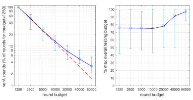
(a)                                                         (b)

Figure 11: Effect of varying the VERACITY round budget on (a) the number of verification rounds; and (b) a normalised measure of the overall testing budget (see main text for details). The plots show mean values and ranges over 10 randomly selected verification scenarios .

6.4 Research question RQ3

The round testing budget $\mathit{rbudget}$ is a key parameter of VERACITY. Large $\mathit{rbudget}$ values all the component observations needed to complete the verification of the nonfunctional requirements acquired in a small number of verification rounds. VERACITY limited opportunity to meaningfully adapt its partitioning of the round budget to the system and requirements being verified. Small $\mathit{rbudget}$ values are equally undesirable yield only a few additional observations in each round. such, they insufficient information to properly guide the round-budget partitioning in the early verification rounds, large numbers of verification rounds, can be computationally expensive because of the formal verification with confidence intervals step of VERACITY.

To analyse these effects of $\mathit{rbudget}$, we randomly selected five of the TAS verification scenarios and five of the WebApp verification scenarios from Section 6.2, and we used VERACITY to verify the nonfunctional requirements of the two systems for each round budget value in the set $\mathit{RB}=\{1250,2500,5000,10000,20000,$ $40000,80000\}$. The experimental results are presented in Figure 11. First, the graph from Figure 11(a) shows the The dashed line from this graph shows what the “ideal” effect of increasing the round budget would look like, i.e., a halving of the number of verification rounds each time when $\mathit{rbudget}$ is doubled, from the baseline of $100\%$ for $\mathit{rbudget}=1250$ to $50\%$ of that baseline for $\mathit{rbudget}=2500$, $25\%$ for $\mathit{rbudget}=5000$, etc. In reality, the number of verification rounds is increasingly above the ideal value as $\mathit{rbudget}$ grows, until it is above this ideal value for all 10 verification scenarios both for $\mathit{rbudget}=40000$ and for $\mathit{rbudget}=80000$. This indicates that very large $\mathit{rbudget}$ values increase the overall testing budgets required by VERACITY—a finding that is further confirmed by Figure 11(b), which shows how the overall testing budget necessary to complete the verification grows with $\mathit{rbudget}$.

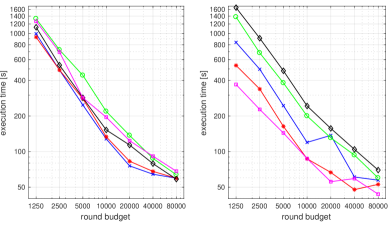
(a) TAS                                                (b) WebApp

Figure 12: Effect of varying the round budget on the VERACITY execution time (experiments carried out on a c5.2xlarge Windows Server 2019 Amazon EC2 instance with 3.00GHz Intel(R) Xeon(R) Platinum 8124M CPU, and 16 GB of memory ).

To summarise the very different overall testing budgets required for our 10 randomly selected verification scenarios in a consistent way, Figure 11(b) considers the overall testing budgets $b_{1}$, $b_{2}$, …, $b_{7}$ associated with each verification scenario and the seven $\mathit{rbudget}$ values from $\mathit{RB}$, finds $b_{\mathsf{max}}=\max\{b_{1},b_{2},\ldots,b_{7}\}$, and computes the percentages of $b_{\mathsf{max}}$ that $b_{1}$, $b_{2}$, …, $b_{7}$ correspond to, i.e., $\mathit{pb}_{1}=100b_{1}/b_{\mathsf{max}}$, $\mathit{pb}_{2}=100b_{2}/b_{\mathsf{max}}$, …, $\mathit{pb}_{7}=100b_{7}/b_{\mathsf{max}}$. These “normalised” budgets show the round budget for which VERACITY requires the highest overall testing budget (e.g., $\mathit{pb}_{7}=100$ means that the highest overall testing budget is needed when $\mathit{rbudget}=80000$), and how the testing budgets for other $\mathit{rbudget}$ values compare to that (e.g., $\mathit{pb}_{1}=75$ means that the overall testing budget for $\mathit{rbudget}=1250$ is 75% of the highest overall testing budget). Figure 11(b) shows how the mean of these normalised budgets increases from $\mathit{pb}_{1}=75.5\%$ for $\mathit{rbudget}=1250$ to $\mathit{pb}_{7}=97\%$ for $\mathit{rbudget}=80000$. The variability of the budget values is very large across the 10 verification scenarios from our experiments, except for the largest round budget $\mathit{rbudget}=80000$, which indicates that this round budget is consistently too large across the majority of the scenarios.

While the effects of using very large $\mathit{rbuget}$ values are clear in Figure 11, noticing the effects of small $\mathit{rbuget}$ values requires a more careful analysis of the experimental results. A first observation we can make is that the experiments with the smallest $\mathit{rbudget}$ values of $1250$, $2500$ and $5000$ used the largest number of verification rounds (as expected, see Figure 11a) without delivering smaller mean overall testing budgets than the experiments for $\mathit{rbudget}=10000$ (see Figure 11b). In fact, the numerical results show a very slight decrease in the mean overall testing budgets from $75.7\%$ for $\mathit{rbudget}=1250$ to $75.5\%$ for $\mathit{rbudget}=2500$, $75.47\%$ for $\mathit{rbudget}=5000$ and $75.05\%$ for $\mathit{rbudget}=10000$. Thus, 11 small $\mathit{rbudget}$ values, increase the cost of the component testing without enabling VERACITY to adapt its partition of the round budget more effectively.

The second undesirable effect of using small $\mathit{rbudget}$ values is visible in Figure 12, which depicts the end-to-end verification times for each of the five TAS verification scenarios and each of the five WebApp verification scenarios we used for the experiments described in this section. As shown by the logarithmic-scale graphs from this figure, the VERACITY execution times approximately double each time the round budget is halved from $\mathit{rbudget}=10000$ to $\mathit{rbudget}=5000$, to $\mathit{rbudget}=2500$ and, finally, to $\mathit{rbudget}=1250$. Even when VERACITY is used at design time and execution times of close to 30 minutes (for $\mathit{rbudget}=1250$) are acceptable, the results from Figure 11b show that such long execution times yield no benefit, so very small $\mathit{rbudget}$ are not recommended. 122

6.5 Threats to validity

Construct validity threats may arise due to assumptions made when modelling the systems from our case studies. To mitigate these threats, we used models and nonfunctional requirements based on established case studies from the research literature [5, 34, 44].

Internal validity threats may be caused by bias in establishing cause-effect relationships in our experiments. To limit these threats, we assessed VERACITY for large numbers of verification scenarios with randomly generated nonfunctional requirements bounds for each research question and each case study: 378 verification scenarios for research question RQ1, 378 verification scenarios for RQ2, and 70 verification scenarios for RQ3. Furthermore, as explained at the beginning of Section 6.2, we ensured that these experiments included scenarios where the requirements were satisfied, where they were violated, and where some requirements were satisfied and others were violated—both by a wide margin and by a narrow margin. Finally, we enable replication by making all experimental results available on our project’s website.

External validity threats may exist if the verification of the nonfunctional requirements of other software systems cannot be expressed in the format from our problem definition in Section 4.1. We limited these threats by ensuring that VERACITY supports the verification of systems whose behaviour is modelled using parametric Markov chains encoded in the widely used modelling language of the PRISM model checker [30], with nonfunctional requirements specified in the established temporal logic PCTL [26, 27, 28]. Parametric Markov models are increasingly used to model software systems including service-based systems [49], software product lines [50], software controllers of cyber-physical systems [51], and multi-tier software architectures [32]. Nevertheless, additional experiments are needed to establish the applicability and feasibility of VERACITY in domains with characteristics different from those used in our evaluation.

[34, 44]

[51, 52, 53, 54, 55, 56, 57, 58], models not larger than our TAS model (i.e., 10 states) are used for evaluation in five papers, and models smaller than or of the same size as our shopping application model (i.e., 17 states) are used for evaluation in all eight papers. While five papers also use models larger than ours for evaluation, these are not models of software systems with multiple components (to which VERACITY is applicable) but models of algorithms, programs and logical gates, or synthetic models that do not correspond to an actual software system. This analysis (whose detailed results are provided on our project’s website) shows that abstraction allows many software engineering projects to usefully exploit models of similar size to the models used for evaluation in our paper. Nevertheless, larger models are sometimes required, and therefore we carried out an additional case study in which we applied VERACITY to an 18-parameter, 41-state discrete-time Markov chain modelling a larger component-based software system taken from [32]. This case study, reported on our project website https://www.cs.york.ac.uk/tasp/VERACITY, indicates that VERACITY can also handle models with larger numbers of parameters and states than those presented earlier in this section.

7 Related work

Within the past decade, the study of uncertainty in the modelling, analysis and verification of complex systems has attracted significant attention from the research community. As such, the existence of different classes of uncertainty is now widely recognised [59, 60, 21, 61], and the research literature provides multiple definitions of uncertainty. Most of these definitions classify uncertainties depending on their: (i) level (ranging from determinism to complete ignorance); (ii) nature (aleatory or epistemic); and (iii) source (in the structure or parameters of models, associated with changes in the operational environment or with the dynamics in the availability of resources, or due to changes in the user goals) [61, 62, 63, 21].

When dealing with the verification of performance, reliability, or other nonfunctional requirements, the term uncertainty is often defined in terms of aleatory and epistemic uncertainty. The aleatory variability of parameters and indices is typically captured using stochastic modelling notations, while the epistemic uncertainty, which refers to the behavior of system portions that are intrinsically unknown, requires ad-hoc methods.

The common goal of these methods is to introduce analysis methodologies able to produce satisfactory results even in presence of such types of uncertainty. For example, [64, 65, 66] propose methods that can be used at design time, to identify software architectures, configurations or component compositions that satisfy a given set of nonfunctional requirements. These approaches take into account the epistemic uncertainty associated with the parameters of models, and use probability distributions to model this uncertainty. To this end, they obtain samples of the uncertain parameter values, and evaluate the robustness of a software system under uncertainty by running Monte-Carlo simulations that use these empirical probability distributions.

More recently, [67] focuses on understanding the influence of configuration options on performance and proposes an approach based on probabilistic programming that explicitly models uncertainty for option influences and provides both a scalar and a confidence interval for each prediction of a configuration’s performance. A method that uses mathematical formulas for incorporating and evaluating epistemic uncertainty of the input parameters of queueing models is presented in [68]. A similar approach to the study of uncertainty propagation in reliability models is introduced in [69].

A different philosophy in dealing with uncertainty involves the adoption of self-adaptation in software systems. The number of studies that consider uncertainty in self-adaptive systems has increased in recent years. A typical example is the use of probabilistic run-time models, such as Markov decision processes [70, 71] and parametric stochastic models [72] to reason about uncertainty and change when making adaptation decisions. The approaches introduced in [73, 74] employ self-adaptation to cope with uncertainty. The approach from [73] proposes a combination of adaptation and evolution of the software to make its behavior resilient to uncertainty, which in turn entails that the software system is sustainable, while [74] focuses on the uncertainty surrounding the execution of cyber-physical production systems. A different approach can be found in [75], where a control-theoretic approach is adopted to handle uncertainty in self-adaptive software systems. Furthermore, the need for software systems to operate well under the existing uncertainties is among the main waves that have advanced the research on self-adaptive systems [76], although a perpetual assurance of goal satisfaction in self-adaptive systems is still an open research challenge [77]. Most of these results consider uncertainty in the decision-making process and propose adaptation approaches that guarantee the quality requirements under different and (possibly) unknown types of changes.

Our work lies in the area of the reduction of parametric epistemic uncertainty and introduces an adaptive uncertainty reduction heuristic for performance and dependability software engineering. The proposed heuristic is integrated into a new iterative approach that exploits the adoption of formal verification with confidence intervals.

One of the key aspects of the proposed approach consists of the identification of the system component for which additional data—to be obtained through testing—are needed. The selection of components to be tested in each iteration is based on a combination of factors that include the sensitivity of the model to variations in the parameters of different components, and the overheads of unit-testing each of these components. Reducing the cost of the (reliability) testing phase by selecting key components to test is a topic that has been analysed in the literature. For example, [78] tackles the question “When to stop testing” by focusing on reliability and discussing the challenges and the potentials related to existing software reliability models. Classical approaches in this domain are based on operational profile [79], however operational profile is often unknown and subject to changes. To overcome this problem, [80] proposes an adapting testing schema that iteratively learns from test execution results as they become available, and, based on them, allocates test cases to the most sensible parts. The assessment is then performed adopting a second sampling strategy that provides the interval estimate of the reliability computed during testing. A different approach that focuses on the allocation of testing resources under uncertain conditions is presented in [81]. In this approach, a multi-objective debug-aware and robust optimization problem under uncertainty of data is used to evaluate of alternative trade-offs among reliability, cost, and release time.

Compared to these approaches, VERACITY has the major advantage that it uses formal quantitative verification to compute confidence intervals for the relevant nonfunctional properties of the system under verification. As such, our approach mitigates the risk of generating inaccurate single-point estimates for these properties. Furthermore, its use of Markov models makes VERACITY applicable to multiple classes of systems for which such models are extensively used, as detailed in Section 6.5.

8 Conclusion

We presented VERACITY, a tool-supported approach for the efficient verification of nonfunctional requirements under uncertainty. VERACITY operates by acquiring information about the components of the verified system through testing them individually over a number of verification rounds. A user-defined testing budget specifies the amount of testing performed in each round, and the partition of this budget among system components is adapted from one round to the next in order complete the verification process with a low overall testing cost. The heuristic used to compute this adaptive partition considers factors such as the sensitivity of the verified requirements to the parameters associated with different components, and the different cost (e.g., time, price or risk) of testing these components. The evaluation of VERACITY in case studies from the areas of service-based systems and web applications showed that, on average, it significantly reduces the overall testing cost required to complete the verification process compared to uniformly partitioning the testing budget across all system components.

In future work, we plan to expand the set of factors underpinning our VERACITY round-budget partitioning, in order to further improve its efficiency. One such additional factor that we are considering is the level of epistemic uncertainty associated with each component: in each round, a larger fraction of the testing budget should be allocated to components with higher levels of epistemic uncertainty, i.e., to those for which fewer observations are already available. We envisage that augmenting our heuristic with this factor will extend the applicability of VERACITY to verification scenarios in which observations about a subset of the system components are already available at the beginning of the verification process (e.g., from previous testing of those components), and we plan to carry out additional case studies to validate this hypothesis.

Another important direction of future research for our project is to consider the scenario in which  some of the parameters that the verified requirements depend on are associated with the operational profile of the system, i.e., with parameters whose epistemic uncertainty cannot be lowered by testing the components of the system. examples of such parameters include the number of requests received by a web server in one hour, and the probabilities of these requests being of different types. To some extent, VERACITY could handle this scenario by associating such parameters with an “operational profile component” that is assigned an infinite testing cost. Because this “component” will never be tested, the verification problem may be undecidable, in which case VERACITY will (correctly) terminate with a ‘budget exhausted’ outcome. However, this outcome will only be produced after significant testing effort, some of which could be avoidable by noticing—before using all the testing budget—that the operational profile uncertainty renders the verification problem undecidable. We plan to extend VERACITY with the ability to report an ‘undecidable’ outcome (without exhausting the testing budget) in this important verification scenario.

(4)

Appendix A

Markov chain construction from UML activity diagrams

A parametric discrete-time Markov chain (1) can be derived from the UML activity diagram of a software system by following the step-by-step process summarised below:

1. Construct the state set $S$ consisting of a state for each activity node from the UML activity diagram, plus an initial state $s_{0}$ and an “end” state $s_{\mathsf{end}}$ associated with the initial and final nodes of the activity diagram, respectively. For each state $s\in S$, let $\mathit{node}(s)$ represent the activity diagram node corresponding to state $s$.

2. Set $\mathbf{P}(s,s^{\prime})=1.0$ for every pair of states $s,s^{\prime}\in S$ for which the node reached immediately after $\mathit{node}(s)$ in the activity diagram (i.e., without traversing activity diagram nodes associated with states from $S\setminus\{s,s^{\prime}\}$) is always $\mathit{node}(s^{\prime})$.

3. Set $\mathbf{P}(s_{\mathsf{end}},s_{\mathsf{end}})=1.0$.

4. Associate an unknown transition probability $\mathbf{P}(s,s^{\prime})$ with each pair of states $s,s^{\prime}\in S$ for which $\mathit{node}(s^{\prime})$ can be reached from $\mathit{node}(s)$ by traversing only decision nodes from the activity diagram.

5. Set $\mathbf{P}(s,s^{\prime})=0$ for every other pair of states $s,s^{\prime}\!\in\!S$.

6. Assemble the atomic proposition set

   $$\mathit{AP}\!=\!\{\mathit{start},\mathit{end}\}\cup\{\mathit{name}(\mathit{node}(s))\!\mid\!s\!\in\!S\setminus\{s_{0},s_{\mathsf{end}}\}\}$$

   where $\mathit{name}(\mathit{node}(s))$ is a unique name for the activity node $node(s)$.

7. Set $L(node(s))=\mathit{name}(\mathit{node}(s))$ for every state $s\in S\setminus\{s_{0},s_{\mathsf{end}}\}$, $L(s_{0})=\mathit{start}$, and $L(s_{\mathsf{end}})=\mathit{end}$.

Further details about this process are available in [35, 36].

References

D. Ameller, X. Franch, C. Gómez, S. Martínez-Fernández, J. Araujo, S. Biffl, J. Cabot, V. Cortellessa, D. Méndez, A. Moreira, H. Muccini, A. Vallecillo, M. Wimmer, V. Amaral, W. Bühm, H. Bruneliere, L. Burgueño, M. Goulão, S. Teufl, L. Berardinelli, Dealing with non-functional requirements in model-driven development: A survey, IEEE Transactions on Software Engineering (2019) 1–1.doi:10.1109/TSE.2019.2904476.

L. Chung, B. A. Nixon, E. Yu, J. Mylopoulos, Non-functional requirements in software engineering, Vol. 5, Springer Science & Business Media, 2012.

R. Calinescu, L. Grunske, M. Kwiatkowska, R. Mirandola, G. Tamburrelli, Dynamic QoS management and optimization in service-based systems, IEEE Transactions on Software Engineering 37 (3) (2011) 387–409.

S. Gallotti, C. Ghezzi, R. Mirandola, G. Tamburrelli, Quality prediction of service compositions through probabilistic model checking, in: International Conference on the Quality of Software Architectures, Springer, 2008, pp. 119–134.

I. Krka, L. Golubchik, N. Medvidovic, Probabilistic automata for architecture-based reliability assessment, in: ICSE Workshop on Quantitative Stochastic Models in the Verification and Design of Software Systems, 2010, pp. 17–24. doi:10.1145/1808877.1808881.

K. Johnson, R. Calinescu, S. Kikuchi, An incremental verification framework for component-based software systems, in: the 16th International ACM Sigsoft Symposium on Component-Based Software Engineering, ACM, 2013, pp. 33–42.

M. A. Marsan, G. Balbo, G. Conte, S. Donatelli, G. Franceschinis, Modelling with generalized stochastic Petri nets, ACM SIGMETRICS Performance Evaluation Review 26 (2) (1998) 2. doi:10.1145/288197.581193.

D. Perez-Palacin, R. Mirandola, J. Merseguer, QoS and energy management with Petri nets: A Self-adaptive framework, Journal of Systems and Software 85 (12) (2012) 2796–2811. doi:10.1016/j.jss.2012.04.077.

A. Filieri, C. S. Pasareanu, W. Visser, Reliability analysis in symbolic pathfinder, in: 35th International Conference on Software Engineering (ICSE), IEEE, 2013, pp. 622–631. doi:10.1109/ICSE.2013.6606608.

R. Calinescu, K. Johnson, Y. Rafiq, Developing self-verifying service-based systems, in: 28th IEEE/ACM International Conference on Automated Software Engineering, IEEE, 2013, pp. 734–737. doi:10.1109/ASE.2013.6693145.

R. Calinescu, C. Ghezzi, K. Johnson, M. Pezzé, Y. Rafiq, G. Tamburrelli, Formal verification with confidence intervals to establish quality of service properties of software systems, IEEE Transactions on Reliability 65 (1) (2015) 107–125.

C. Paterson, R. Calinescu, Observation-enhanced QoS analysis of component-based systems, IEEE Transactions on Software Engineering 46 (05) (2020) 526–548. doi:10.1109/TSE.2018.2864159.

A. K. Akobeng, Confidence intervals and p-values in clinical decision making, Acta Pædiatrica 97 (8) (2008) 1004–1007.

B. R. Kirkwood, J. A. Sterne, Essential medical statistics, John Wiley & Sons, 2010.

J. R. Benjamin, C. A. Cornell, Probability, statistics, and decision for civil engineers, Courier Corporation, 2014.

J. M. Aughenbaugh, C. J. Paredis, The value of using imprecise probabilities in engineering design, Journal of Mechanical Design 128 (4) (2006) 969–979.

J.-B. du Prel, G. Hommel, B. Röhrig, M. Blettner, Confidence interval or p-value? (part 4 of a series on evaluation of scientific publications), Deutsches Ärzteblatt International 106 (19) (2009) 335.

M. J. Gardner, D. G. Altman, Confidence intervals rather than P values: estimation rather than hypothesis testing, British Medical Journal 292 (6522) (1986) 746–750. doi:10.1136/bmj.292.6522.746.

D. Perez-Palacin, R. Mirandola, Uncertainties in the modeling of self-adaptive systems: a taxonomy and an example of availability evaluation, in: 5th ACM/SPEC International Conference on Performance Engineering, ACM, 2014, pp. 3–14.
URL https://doi.org/10.1145/2568088.2568095

R. Calinescu, K. Johnson, C. Paterson, FACT: A probabilistic model checker for formal verification with confidence intervals, in: International Conference on Tools and Algorithms for the Construction and Analysis of Systems, Springer, 2016, pp. 540–546.

E. Daka, G. Fraser, A survey on unit testing practices and problems, in: 2014 IEEE 25th International Symposium on Software Reliability Engineering, 2014, pp. 201–211. doi:10.1109/ISSRE.2014.11.

The European Mathematical Society, The Encyclopedia of Mathematics (2020).
URL https://encyclopediaofmath.org/wiki/Rational_function

C. Daws, Symbolic and parametric model checking of discrete-time Markov chains, in: International Colloquium on Theoretical Aspects of Computing, 2005, pp. 280–294. doi:10.1007/978-3-540-31862-0_21.

S. Andova, H. Hermanns, J.-P. Katoen, Discrete-time rewards model-checked, in: International Conference on Formal Modeling and Analysis of Timed Systems, Springer, 2004, pp. 88–104. doi:10.1007/978-3-540-40903-8_8.

F. Ciesinski, M. Größer, On probabilistic computation tree logic, in: C. Baier, B. R. Haverkort, H. Hermanns, J.-P. Katoen, M. Siegle (Eds.), Validation of Stochastic Systems: A Guide to Current Research, Springer, 2004, pp. 147–188. doi:10.1007/978-3-540-24611-4_5.

H. Hansson, B. Jonsson, A logic for reasoning about time and reliability, Formal Aspects of Computing 6 (5) (1994) 512–535. doi:10.1007/BF01211866.

E. M. Hahn, H. Hermanns, B. Wachter, L. Zhang, PARAM: A model checker for parametric markov models, in: Computer Aided Verification, Springer, 2010, pp. 660–664. doi:10.1007/978-3-642-14295-6_56.

M. Kwiatkowska, G. Norman, D. Parker, PRISM 4.0: Verification of probabilistic real-time systems, in: Computer Aided Verification, Springer, 2011, pp. 585–591. doi:10.1007/978-3-642-22110-1_47.

C. Dehnert, S. Junges, J.-P. Katoen, M. Volk, A storm is coming: A modern probabilistic model checker, in: 29th International Conference on Computer Aided Verification (CAV), 2017, pp. 592–600. doi:10.1007/978-3-319-63390-9_31.

R. Calinescu, C. A. Paterson, K. Johnson, Efficient parametric model checking using domain knowledge, IEEE Transactions on Software Engineering 47 (6) (2021) 1114–1133. doi:10.1109/TSE.2019.2912958.

X. Fang, R. Calinescu, S. Gerasimou, F. Alhwikem, Fast parametric model checking through model fragmentation, in: 43rd IEEE/ACM International Conference on Software Engineering, 2021, pp. 835–846.

L. Baresi, D. Bianculli, C. Ghezzi, S. Guinea, P. Spoletini, Validation of web service compositions, IET Software 1 (6) (2007) 219–232. doi:10.1049/iet-sen:20070027.

R. Calinescu, Y. Rafiq, Using intelligent proxies to develop self-adaptive service-based systems, in: 2013 International Symposium on Theoretical Aspects of Software Engineering, IEEE, 2013, pp. 131–134.

C. Ghezzi, L. S. Pinto, P. Spoletini, G. Tamburrelli, Managing non-functional uncertainty via model-driven adaptivity, in: 2013 35th International Conference on Software Engineering (ICSE), IEEE, 2013, pp. 33–42.

Z. W. Birnbaum, On the importance of different components in a multicomponent system, in: P. R. Krishnaiah (Ed.), Multivariate Analysis II, Academic Press, New York, 1969.

R. E. Barlow, F. Proschan, Importance of system components and fault tree events, Stochastic Processes and Their Applications 3 (2) (1975) 153–173.

V. B. Kampenes, T. Dybå, J. E. Hannay, D. I. Sjøberg, A systematic review of effect size in software engineering experiments, Information and Software Technology 49 (11-12) (2007) 1073–1086.

B. Kitchenham, L. Madeyski, D. Budgen, J. Keung, P. Brereton, S. Charters, S. Gibbs, A. Pohthong, Robust statistical methods for empirical software engineering, Empirical Software Engineering 22 (2) (2017) 579–630.

L. Madeyski, B. Kitchenham, Effect sizes and their variance for ab/ba crossover design studies, Empirical Software Engineering 23 (4) (2018) 1982–2017.

L. Madeyski, Test-driven development: An empirical evaluation of agile practice, Springer Science & Business Media, 2009.

R. J. Grissom, J. J. Kim, Effect sizes for research: A broad practical approach., Lawrence Erlbaum Associates Publishers, 2005.

A. Filieri, C. Ghezzi, G. Tamburrelli, A formal approach to adaptive software: continuous assurance of non-functional requirements, Formal Aspects of Computing 24 (2) (2012) 163–186.

A. Fabijan, P. Dmitriev, C. McFarland, L. Vermeer, H. Holmström Olsson, J. Bosch, Experimentation growth: Evolving trustworthy A/B testing capabilities in online software companies, Journal of Software: Evolution and Process 30 (12) (2018) e2113.

R. Kohavi, R. Longbotham, Online controlled experiments and A/B testing, Encyclopedia of machine learning and data mining 7 (8) (2017) 922–929.

D. Siroker, P. Koomen, A/B testing: The most powerful way to turn clicks into customers, John Wiley & Sons, 2013.

H. Muccini, M. Dias, D. J. Richardson, Software architecture-based regression testing, Journal of Systems and Software 79 (10) (2006) 1379–1396, architecting Dependable Systems. doi:https://doi.org/10.1016/j.jss.2006.02.059.
URL https://www.sciencedirect.com/science/article/pii/S0164121206001361

S. Gerasimou, R. Calinescu, G. Tamburrelli, Synthesis of probabilistic models for quality-of-service software engineering, Automated Software Engineering 25 (4) (2018) 785–831.

C. Ghezzi, A. M. Sharifloo, Model-based verification of quantitative non-functional properties for software product lines, Information and Software Technology 55 (3) (2013) 508–524.

R. Calinescu, D. Weyns, S. Gerasimou, M. U. Iftikhar, I. Habli, T. Kelly, Engineering trustworthy self-adaptive software with dynamic assurance cases, IEEE Transactions on Software Engineering 44 (11) (2017) 1039–1069.

G. Su, D. S. Rosenblum, G. Tamburrelli, Reliability of run-time quality-of-service evaluation using parametric model checking, in: 2016 IEEE/ACM 38th International Conference on Software Engineering (ICSE), 2016, pp. 73–84.

J. M. Franco, F. Correia, R. Barbosa, M. Zenha-Rela, B. Schmerl, D. Garlan, Improving self-adaptation planning through software architecture-based stochastic modeling, Journal of Systems and software 115 (2016) 42–60.

Y. R. S. Llerena, M. Böhme, M. Brünink, G. Su, D. S. Rosenblum, Verifying the long-run behavior of probabilistic system models in the presence of uncertainty, in: Proceedings of the 2018 26th ACM Joint Meeting on European Software Engineering Conference and Symposium on the Foundations of Software Engineering, 2018, pp. 587–597.

X. Wang, J. Sun, Z. Chen, P. Zhang, J. Wang, Y. Lin, Towards optimal concolic testing, in: Proceedings of the 40th International Conference on Software Engineering, 2018, pp. 291–302.

H. Nakagawa, H. Toyama, T. Tsuchiya, Expression caching for runtime verification based on parameterized probabilistic models, Journal of Systems and Software 156 (2019) 300–311.

H. Afzal, M. R. Mufti, I. Awan, M. Yousaf, Performance analysis of radio spectrum for cognitive radio wireless networks using discrete time Markov chain, Journal of Systems and Software 151 (2019) 1–7.

G. Su, Y. Feng, T. Chen, D. S. Rosenblum, Asymptotic perturbation bounds for probabilistic model checking with empirically determined probability parameters, IEEE Transactions on Software Engineering 42 (7) (2016) 623–639. doi:10.1109/TSE.2015.2508444.

A. J. Ramirez, A. C. Jensen, B. H. C. Cheng, A taxonomy of uncertainty for dynamically adaptive systems, in: Proceedings of the 7th International Symposium on Software Engineering for Adaptive and Self-Managing Systems, SEAMS ’12, IEEE Press, Piscataway, NJ, USA, 2012, pp. 99–108.
URL http://dl.acm.org/citation.cfm?id=2666795.2666812

H. Giese, N. Bencomo, L. Pasquale, A. J. Ramirez, P. Inverardi, S. Wätzoldt, S. Clarke, Living with uncertainty in the age of runtime models, in: N. Bencomo, R. France, B. H. C. Cheng, U. Aßmann (Eds.), Models@run.time: Foundations, Applications, and Roadmaps, Springer International Publishing, Cham, 2014, pp. 47–100.

W. Walker, P. Harremoes, J. Romans, J. van der Sluus, M. van Asselt, P. Janssen, M. Krauss, Defining uncertainty. a conceptual basis for uncertainty management in model-based decision support, Integrated Assessment 4 (1) (2003) 5–17.

D. Garlan, Software engineering in an uncertain world, in: Future of Software Engineering Research, ACM, 2010, pp. 125–128.

N. Esfahani, S. Malek, Uncertainty in self-adaptive software systems, in: Software Engineering for Self-Adaptive Systems II. Lecture Notes in Computer Science, vol 7475, Springer, 2013, pp. 214–238. doi:https://doi.org/10.1007/978-3-642-35813-5_9.

C. Trubiani, I. Meedeniya, V. Cortellessa, A. Aleti, L. Grunske, Model-based performance analysis of software architectures under uncertainty, in: the 9th international ACM Sigsoft conference on Quality of software architectures, ACM, 2013, pp. 69–78. doi:10.1145/2465478.2465487.

I. Meedeniya, I. Moser, A. Aleti, L. Grunske, Architecture-based reliability evaluation under uncertainty, in: the Joint ACM SIGSOFT Conference – QoSA and ACM SIGSOFT Symposium – ISARCS on Quality of Software Architectures – QoSA and Architecting Critical Systems – ISARCS, ACM, 2011, pp. 85–94. doi:10.1145/2000259.2000275.

I. Meedeniya, A. Aleti, L. Grunske, Architecture-driven reliability optimization with uncertain model parameters, Journal of Systems and Software 85 (10) (2012) 2340–2355.

J. Dorn, S. Apel, N. Siegmund, Mastering uncertainty in performance estimations of configurable software systems, in: 2020 35th IEEE/ACM International Conference on Automated Software Engineering (ASE), 2020, pp. 684–696.

F. Antonelli, V. Cortellessa, M. Gribaudo, R. Pinciroli, K. S. Trivedi, C. Trubiani, Analytical modeling of performance indices under epistemic uncertainty applied to cloud computing systems, Future Generation Computer Systems 102 (2020) 746 – 761. doi:https://doi.org/10.1016/j.future.2019.09.006.

K. Mishra, K. S. Trivedi, Closed-form approach for epistemic uncertainty propagation in analytic models, in: T. Dohi, T. Nakagawa (Eds.), Stochastic Reliability and Maintenance Modeling: Essays in Honor of Professor Shunji Osaki on his 70th Birthday, Springer London, London, 2013, pp. 315–332. doi:10.1007/978-1-4471-4971-2_14.

R. Calinescu, M. Autili, J. Cámara, A. Di Marco, S. Gerasimou, P. Inverardi, A. Perucci, N. Jansen, J.-P. Katoen, M. Kwiatkowska, O. J. Mengshoel, R. Spalazzese, M. Tivoli, Synthesis and verification of self-aware computing systems, in: S. Kounev, J. O. Kephart, A. Milenkoski, X. Zhu (Eds.), Self-Aware Computing Systems, Springer, 2017, pp. 337–373.

G. A. Moreno, J. Camara, D. Garlan, B. Schmerl, Proactive self-adaptation under uncertainty: A probabilistic model checking approach, in: Foundations of Software Engineering, ACM, 2015, pp. 1–12.

R. Calinescu, M. Ceska, S. Gerasimou, M. Kwiatkowska, N. Paoletti, Efficient synthesis of robust models for stochastic systems, Journal of Systems and Software 143 (2018) 140–158.

D. Weyns, M. Caporuscio, B. Vogel, A. Kurti, Design for sustainability = runtime adaptation $\cup$ evolution, in: the 2015 European Conference on Software Architecture Workshops, ACM, 2015, pp. 62:1–62:7. doi:10.1145/2797433.2797497.

A. Musil, J. Musil, D. Weyns, T. Bures, H. Muccini, M. Sharaf, Patterns for self-adaptation in cyber-physical systems, in: Multi-disciplinary engineering for cyber-physical production systems, Springer, 2017, pp. 331–368.

S. Shevtsov, D. Weyns, M. Maggio, SimCA*: A control-theoretic approach to handle uncertainty in self-adaptive systems with guarantees, ACM Transactions on Autonomous and Adaptive Systems 13 (4) (2019) 1–34. doi:10.1145/3328730.

D. Weyns, Software engineering of self-adaptive systems: an organised tour and future challenges, Chapter in Handbook of Software Engineering, Springer, 2017.

D. Weyns, N. Bencomo, R. Calinescu, J. Camara, C. Ghezzi, V. Grassi, L. Grunske, P. Inverardi, J.-M. Jezequel, S. Malek, et al., Perpetual assurances for self-adaptive systems, in: Software Engineering for Self-Adaptive Systems III. Assurances, Springer, 2017, pp. 31–63.

M. Garg, R. Lai, S. J. Huang, When to stop testing: a study from the perspective of software reliability models, IET Software 5 (2011) 263–273(10).
URL https://digital-library.theiet.org/content/journals/10.1049/iet-sen.2010.0007

J. D. Musa, The operational profile, in: S. Özekici (Ed.), Reliability and Maintenance of Complex Systems, Springer Berlin Heidelberg, Berlin, Heidelberg, 1996, pp. 333–344.

D. Cotroneo, R. Pietrantuono, S. Russo, RELAI testing: A technique to assess and improve software reliability, IEEE Trans. Software Eng. 42 (5) (2016) 452–475. doi:10.1109/TSE.2015.2491931.

R. Pietrantuono, P. Potena, A. Pecchia, D. Rodríguez, S. Russo, L. F. Sanz, Multiobjective testing resource allocation under uncertainty, IEEE Trans. Evol. Comput. 22 (3) (2018) 347–362. doi:10.1109/TEVC.2017.2691060.