Asymptotic behavior of the steady Prandtl equation

Abstract.

We study the asymptotic behavior of the Oleinik’s solution to the steady Prandtl equation when the outer flow $U(x)=1$. Serrin proved that the Oleinik’s solution converges to the famous Blasius solution $\bar{u}$ in $L^{\infty}_{y}$ sense as $x\rightarrow+\infty$. The explicit decay estimates of $u-\bar{u}$ and its derivatives were proved by Iyer[ARMA 237(2020)] when the initial data is a small localized perturbation of the Blasius profile. In this paper, we prove the explicit decay estimate of $\|u(x,y)-\bar{u}(x,y)\|_{L^{\infty}_{y}}$ for general initial data with exponential decay. We also prove the decay estimates of its derivatives when the data has an additional concave assumption. Our proof is based on the maximum principle technique. The key ingredient is to find a series of barrier functions.

1. Introduction

We study the steady Prandtl equation

(1.1) $$\left\{\begin{aligned} &u\partial_{x}u+v\partial_{y}u-\partial_{y}^{2}u=\frac{dp}{dx},\quad(x,y)\in\mathbf{R}_{+}\times\mathbf{R}_{+},\\ &\partial_{x}u+\partial_{y}v=0,\\ &u|_{x=0}=u_{0}(y),\quad u|_{y=0}=v|_{y=0}=0,\\ &\displaystyle\lim_{y\to+\infty}u(x,y)=U(x).\end{aligned}\right.$$

Here $(u,v)$ is the velocity and the outer flow $(U(x),p(x))$ satisfies the Bernoulli’s law:

$$U(x)U^{\prime}(x)+p^{\prime}(x)=0.$$

In this paper, we consider the case when the gradient of pressure $p^{\prime}(x)=0$. Thus, the outer flow $U(x)$ is a constant in this case. For simplicity, we take $U\equiv 1.$

Let us introduce the Von Mises transformation $(x,\psi)$ defined by

(1.2) $$x=x,\,\,\psi=\psi(x,y)=\int_{0}^{y}u(x,y^{\prime})dy^{\prime}.$$

Introduce the new unknown $w(x,\psi)=u(x,y)^{2}.$ A direct calculation shows that

(1.3) $$\begin{split}&2\partial_{y}u=\partial_{\psi}w,\quad 2\partial^{2}_{y}u=\sqrt{w}\partial^{2}_{\psi}w.\end{split}$$

Hence, the Prandtl system is reduced to a parabolic type equation(view $x$ as time direction):

(1.4) $$\partial_{x}w=\sqrt{w}\partial_{\psi}^{2}w$$

along with the boundary conditions

(1.5) $$\begin{split}&w(x,0)=0,\quad w(0,\psi)=w_{0}(\psi),\\ &w(x,\psi)\rightarrow 1\quad\text{as}\,\,\psi\rightarrow+\infty.\end{split}$$

Based on the Von Mises transformation and maximum principle technique, Oleinik proved the following existence and uniqueness result of classical solution(see Theorem 2.1.1 in [8]).

Theorem 1.1.

(Oleinik) If $\frac{dp}{dx}=0$ and the initial data $u_{0}$ satisfies

(1.6) $$\begin{split}&u_{0}(y)\in C_{b}^{2,\alpha}\big{(}[0,+\infty)\big{)}(\alpha>0),\quad u_{0}(0)=0,\,\,u^{\prime}_{0}(0)>0,\\ &u_{0}(y)>0\,\,\text{for}\,\,y\in(0,+\infty),\,\,u^{\prime\prime}_{0}(y)=O(y^{2}),\end{split}$$

then the steady Prandtl equation (1.1) admits a global-in-$x$ solution $u_{0}\in C^{1}(\mathbf{R}_{+}\times\mathbf{R}_{+})$ with the following properties: for any $X>0,$

1. $u$ is bounded and continuous in $[0,X]\times\mathbf{R}_{+};$

2. $u(x,y)>0$ for $y>0;$

3. $u_{y},u_{yy}$ are bounded and continuous in $[0,X]\times\mathbf{R}_{+}$;

4. $v,v_{y},u_{x}$ are locally bounded and continuous in $[0,X]\times\mathbf{R}_{+}.$

In fact, Theorem 2.1.1 in [8] showed that in the case of favorable pressure gradient $p^{\prime}(x)\leq 0$, the global-in-$x$ solutions exist; while in the case of adverse pressure gradient $p^{\prime}(x)>0,$ only local-in-$x$ solutions exist.

Recently, in the case of favorable pressure gradient, Guo and Iyer [4] proved the higher regularity of the solution through the energy method, and the authors proved the global-in-$x$ $C^{\infty}$ regularity up to the boundary $y=0$ using the maximum principle technique [11]. In the case of adverse pressure gradient, Dalibard and Masmoudi [1] as well as Shen and the authors [10] justified the physical phenomenon of boundary layer separation. Let us mention some related works [12, 2, 7] for the unsteady Prandtl equation.

In this paper, we are concerned with the asymptotic behavior of Oleinik’s solution when the outer flow $U(x)=1$. In this case, (1.1) admits a family of self-similar Blasius solutions:

(1.7) $$[\bar{u},\bar{v}]=\Big{[}f^{\prime}(\zeta),\frac{1}{2\sqrt{x+x_{0}}}\{\zeta f^{\prime}(\zeta)-f(\zeta)\}\Big{]},$$

where $\zeta=\frac{y}{\sqrt{x+x_{0}}}$ with $x_{0}>0$ as a free parameter. See section 2.1 for the properties of $f(\zeta)$. For simplicity, we always take $x_{0}=1.$

Serrin [9] proved the following asymptotic behavior of the Oeinik’s solution.

Theorem 1.2.

(Serrin) Let $u$ be a global Oleinik’s solution to (1.1) with $U(x)=1$. Then the asymptotic behavior holds

$$\|u(x,y)-\bar{u}(x,y)\|_{L^{\infty}_{y}}\rightarrow 0\quad\text{as}\quad x\rightarrow+\infty.$$

Recently, Iyer [5] proved the explicit decay estimates of modulated substraction $\phi$ and its derivatives in the Von Mises coordinates when the initial data is a small localized perturbation of the Blasius profile by using the energy method, where

(1.8) $$\begin{split}\phi(x,\psi)&=w(x,\psi)-\bar{w}(x,\psi),\quad\bar{w}=\bar{u}^{2}.\end{split}$$

These estimates play a crucial role in validating the Prandtl’s boundary layer theory [3, 6].

The aim of this paper is to study the asymptotic behavior of the Oleinik’s solution for general initial data. The first main result is stated as follows.

Theorem 1.3.

Let $u$ be a global Oleinik’s solution to (1.1) with $U(x)=1$. Under the additional decay assumption

(1.9) $$|u_{0}(y)-1|\leq C_{4}e^{-y^{2}C_{5}}$$

for some positive constants $C_{4},C_{5}$ with $C_{5}>C_{1}$ where $C_{1}$ is the constant in (2.2), there exist positive constants $C$ and $c$ so that for any $(x,y)\in\mathbf{R}_{+}\times\mathbf{R}_{+}$,

$$|u(x,y)-\bar{u}(x,y)|\leq\frac{C}{\sqrt{x+1}}\ln(x+e)e^{-c\frac{y^{2}}{x+1}}.$$

Remark 1.4.

The decay rate should be optimal in the sense explained on Page 6 in [6].

For the decay estimates of high order derivatives of $u$, we additionally require the initial data to be concave.

Theorem 1.5.

Let $u$ be a global Oleinik’s solution to (1.1) with $U(x)=1$. Under the assumptions (1.9) and

(1.10) $$C_{6}e^{-y^{2}C_{7}}\leq\partial_{y}^{2}u_{0}(y)\leq 0$$

for some positive constants $C_{6},C_{7}$ with $C_{7}>C_{1}$ where $C_{1}$ is the constant in (2.2), there exist positive constants $C,c$ and $N$ so that for any $(x,y)\in(N,+\infty)\times\mathbf{R}_{+}$,

$$-\frac{C}{x+1}e^{-c\frac{y^{2}}{x+1}}\leq\partial_{y}^{2}u(x,y)\leq 0,$$

$$|\partial_{y}(u(x,y)-\bar{u}(x,y))|\leq\frac{C}{(x+1)^{\frac{3}{4}}}\ln(x+e)e^{-c\frac{y^{2}}{x+1}},$$

$$|\partial_{x}u(x,y)|\leq\frac{C}{x+1}e^{-c\frac{y^{2}}{x+1}},\quad|\partial_{xy}u(x,y)|\leq\frac{C}{(x+1)^{\frac{3}{4}}}e^{-c\frac{y^{2}}{x+1}}.$$

Remark 1.6.

These decay estimates mean that $u$ has similar behaviors with the Blasius solution in the large time. It remains unknown whether the concave condition could be removed.

The proof of Theorem 1.3 and Theorem 1.5 is based on decay estimates for $\phi$ and $w$ under the Von Mises coordinates.

Theorem 1.7.

Under the assumptions in Theorem 1.5, there exist positive constants $C$ and $c$ so that for any $(x,\psi)\in\mathbf{R}_{+}\times\mathbf{R}_{+}$,

$$|\phi(x,\psi)|\leq\frac{C}{\sqrt{x+1}}e^{-c\frac{\psi^{2}}{x+1}},\quad|\partial_{\psi}^{2}\phi(x,\psi)|\leq\frac{C}{x+1}e^{-c\frac{\psi^{2}}{x+1}},$$

$$|\partial_{x}\phi(x,\psi)|\leq\frac{C}{x+1}e^{-c\frac{\psi^{2}}{x+1}},\quad|\partial_{\psi}\phi(x,\psi)|\leq\frac{C}{(x+1)^{\frac{3}{4}}}e^{-c\frac{\psi^{2}}{x+1}}.$$

Theorem 1.8.

Under the assumptions in Theorem 1.5, there exist positive constants $C,c$ and $N$ so that for any $(x,\psi)\in(N,+\infty)\times\mathbf{R}_{+}$,

$$|\partial_{\psi x}w(x,\psi)|\leq\frac{C}{(x+1)^{\frac{3}{4}}}e^{-c\frac{\psi^{2}}{x+1}},$$

$$|\partial_{x}^{2}w(x,\psi)|+|\partial_{x}\partial_{\psi}^{2}w(x,\psi)|\leq\frac{C}{(x+1)^{\frac{1}{2}}}e^{-c\frac{\psi^{2}}{x+1}}.$$

The proof of Theorem 1.7 and Theorem 1.8 used the maximum principle technique. The key ingredient is to find a series of barrier functions (with ridges), whose constructions depend on the structure of Blasius profile. In fact, we provide the pointwise estimates including the decay rate with respect to $\psi$ near $\psi=0,$ which is crucial when we derive the decay estimates under the Euler coordinates from the results obtained under the Von Mises coordinates.

2. Blasius profile and Von Mises coordinates

2.1. Blasius profile

The Blasius profile $f(\zeta)$ satisfies

(2.1) $$\begin{split}&\frac{1}{2}ff^{\prime\prime}+f^{\prime\prime\prime}=0,\,\,f(0)=f^{\prime}(0)=0,\\ &f^{\prime}(\zeta)\rightarrow 1\quad\text{and}\quad\frac{f(\zeta)}{\zeta}\rightarrow 1\quad\,\text{as}\,\,\zeta\rightarrow+\infty,\\ &0\leq f^{\prime}(\zeta)\leq 1\quad\text{and}\quad f^{\prime\prime}(\zeta)\geq 0\quad\text{for}\,\,\zeta\geq 0\\ &0<f^{\prime\prime}(0)=b_{0},\quad f^{\prime\prime\prime}(\zeta)<0\quad\text{for}\,\,\zeta>0.\end{split}$$

There exist positive constants $C_{1},C_{2}$ so that

(2.2) $$1-f^{\prime}(\zeta)\sim\zeta^{-1}e^{-\zeta^{2}C_{1}-C_{2}\zeta},\quad f^{\prime\prime}(\zeta)\sim\zeta(1-f^{\prime})\sim e^{-\zeta^{2}C_{1}-C_{2}\zeta},$$

as $\zeta\rightarrow+\infty.$

Lemma 2.1.

It holds that

$$f^{(3)}(0)=0,\quad f^{(4)}(0)=0,\quad f^{(5)}(0)<0.$$

Proof.

By $\frac{1}{2}ff^{\prime\prime}+f^{\prime\prime\prime}=0,$ we have $f^{(3)}(0)=0$ and

(2.3) $$\begin{split}&\frac{1}{2}f^{\prime}f^{\prime\prime}+\frac{1}{2}ff^{(3)}+f^{(4)}=0,\\ &\frac{1}{2}(f^{\prime\prime})^{2}+\frac{1}{2}f^{\prime}f^{(3)}+\frac{1}{2}ff^{(4)}+\frac{1}{2}f^{\prime}f^{(3)}+f^{(5)}=0.\end{split}$$

By (2.1) and evaluating at $\zeta=0,$ the result follows. ∎

2.2. A comparison lemma

Lemma 2.2.

There exist positive constants $c<1$ and $C>1$ depending on $w_{0}$ such that

(2.4) $$c\bar{w}\leq w\leq C\bar{w}\quad\text{in}\quad\mathbf{R}_{+}\times\mathbf{R}_{+}.$$

Proof.

Since $u_{0}(0)=0$ and $u_{0}^{\prime}(0)>0,$ by (1.3),

$$w_{0}(0)=0,\quad\partial_{\psi}w(0,\psi)\sim 1\quad\psi\,\,\text{near}\,\,0,$$

which gives

$$\bar{w}(0,\psi)\sim\psi\sim w(0,\psi)\quad\psi\,\,\text{near}\,\,0.$$

Thanks to $u_{0}(y)>0$ and $\bar{u}(0,y)>0$ for $y>0$, we have $\bar{w}>0$ and $w>0$ for $\psi>0.$ Moreover, $w(x,\psi),\,\,\bar{w}(x,\psi)\rightarrow 1$ as $\psi\rightarrow+\infty$. Hence, away from $0$, both $w_{0}(\psi)$ and $\bar{w}(0,\psi)$ have positive minimum and maximum. Then there exist some positive constants $c<1$ and $1<C$ so that

(2.5) $$cw_{0}(\psi)\leq\bar{w}(0,\psi)\leq Cw_{0}(\psi).$$

Take $c$ and $C$ to be the constants in (2.5). For any positive constant $b,$ we have

$$\partial_{x}(w-b\bar{w})-\sqrt{w}\partial_{\psi}^{2}(w-b\bar{w})=(\sqrt{b}\sqrt{w}-b\sqrt{\bar{w}})\partial_{\psi}^{2}\bar{w}+(b-\sqrt{b})\sqrt{w}\partial_{\psi}^{2}\bar{w},$$

where we note $\partial_{\psi}^{2}\bar{w}<0$ for $\psi>0.$

We first prove that $w-C\bar{w}\leq 0.$ Otherwise, since $w-C\bar{w}=0$ on $\psi=0$, (2.4) holds on $x=0$ due to (2.5), and $w-C\bar{w}\rightarrow 1-C<0$ as $\psi\rightarrow+\infty$, a positive maximum is obtained at some point $(x_{0},\psi_{0})\in(0,x_{0}]\times(0,+\infty)$ with $(w-C\bar{w})(x_{0},\psi_{0})>0$. This implies

$$(\sqrt{w}-\sqrt{C}\sqrt{\bar{w}})(x_{0},\psi_{0})>0.$$

On the other hand, at $(x_{0},\psi_{0}),$

$$\partial_{x}(w-C\bar{w})-\sqrt{w}\partial_{\psi}^{2}(w-C\bar{w})=\sqrt{C}(\sqrt{w}-\sqrt{C}\sqrt{\bar{w}})\partial_{\psi}^{2}\bar{w}+(C-\sqrt{C})\sqrt{w}\partial_{\psi}^{2}\bar{w}<0,$$

which contradicts to the property of maximum point. Hence, $w-C\bar{w}\leq 0.$

The proof of $w-c\bar{w}\geq 0$ is similar. At the negative minimum point, $\sqrt{w}<\sqrt{c}\sqrt{\bar{w}}$ and there holds

$$\partial_{x}(w-c\bar{w})-\sqrt{w}\partial_{\psi}^{2}(w-c\bar{w})=(\sqrt{c}\sqrt{w}-c\sqrt{\bar{w}})\partial_{\psi}^{2}\bar{w}+(c-\sqrt{c})\sqrt{w}\partial_{\psi}^{2}\bar{w}>0,$$

which also leads to a contradiction. ∎

2.3. Von Mises coordinates

By (1.2), we introduce the notation

(2.6) $$y(\psi;u)=\int_{0}^{\psi}\frac{1}{\sqrt{w}(x,\psi^{\prime})}d\psi^{\prime}.$$

In particular, $y(\psi;\bar{u})=\int_{0}^{\psi}\frac{1}{\sqrt{\bar{w}}(x,\psi^{\prime})}d\psi^{\prime},$ corresponds to the Blasius profile. It follows from Lemma 2.2 that there exist positive constants $c$ and $C$ such that

(2.7) $$cy(\psi;\bar{u})\leq y(\psi;u)\leq Cy(\psi;\bar{u}).$$

In what follows, we always denote

(2.8) $$h=\frac{\psi}{\sqrt{x+1}},\quad\zeta=\frac{y(\psi;\bar{u})}{\sqrt{x+1}}.$$

We infer from (1.2) that for $y=y(\psi;\bar{u})$,

$$\psi=\int_{0}^{y}\bar{u}(x,y^{\prime})dy^{\prime}=\sqrt{x+1}\int_{0}^{\zeta}f^{\prime}(\zeta)d\zeta=\sqrt{x+1}f(\zeta),$$

which gives

(2.9) $$h=\frac{\psi}{\sqrt{x+1}}=f(\zeta).$$

Since $f^{\prime\prime}\geq 0,\,f^{\prime\prime}(0)>0$ and $f^{\prime}(0)=0$, it holds that $f^{\prime}(\zeta)>0$ for $\zeta>0,$ and thus $f$ is strictly increasing. Hence, $\zeta\stackrel{{\scriptstyle one\,to\,one}}{{\longleftrightarrow}}h$. By (2.1), there exists a large positive constant $M$ such that

(2.10) $$\frac{1}{2}\zeta\leq\frac{\psi}{\sqrt{x+1}}=f(\zeta)\leq 2\zeta$$

when $\zeta\geq M$ or $h\geq M$.

Since $f^{\prime}(\zeta)\sim\zeta,\,\,f(\zeta)\sim\zeta^{2}$ for $\zeta$ near $0$ due to (2.1), it holds that for any $a>0$,

(2.11) $$c_{a}h\leq\bar{w}(x,\psi)\leq C_{a}h\quad\text{for}\,\,h\leq a.$$

Recall $\bar{w}=\bar{u}^{2}=f^{\prime}(\zeta)^{2}$. By (1.3) and (1.4), we have the following relations which will be frequently used:

(2.12) $$\begin{split}-\partial_{x}\bar{w}=\frac{1}{x+1}ff^{\prime\prime},\quad\partial_{\psi}\bar{w}=\frac{2}{\sqrt{x+1}}f^{\prime\prime}.\end{split}$$

From (2.12), (2.1) and (2.2), it holds hat

(2.13) $$\begin{split}-\partial_{x}\bar{w}&\geq c\frac{1}{x+1}\zeta^{2}\quad\text{for}\quad\zeta\leq 1,\\ -\partial_{x}\bar{w}&\geq c\frac{1}{x+1}\zeta f^{\prime\prime}\quad\text{for}\quad\zeta>1.\end{split}$$

From Lemma 2.1, (2.1) and (2.12), it is easy to see that

Lemma 2.3.

For any fixed $x\in[0,+\infty),$ $-\partial_{x}\bar{w}$ is increasing with respect to $\psi$ and $-\partial_{x}\bar{w}$ is positive for $\psi>0$.

If we use $(\tilde{x},\psi)$ to denote the Von Mises variables to avoid confusion for a while, then it holds that

(2.14) $$\partial_{\tilde{x}}=\partial_{x}-\frac{\int_{0}^{y}\bar{u}_{x}(x,y^{\prime})dy^{\prime}}{\bar{u}}\partial_{y}.$$

2.4. Some properties of $w$

From Theorem 2.1.14, Lemma 2.1.9 and Lemma 2.1.12 in [8] and Lemma 3.1 in [1], we know that

• $\partial_{x}w(x,0)=0.$

• $\displaystyle\lim_{\psi\to+\infty}\partial^{2}_{\psi}w(x,\psi)=0,$ which implies

  (2.15) $$\displaystyle\lim_{\psi\to+\infty}\partial_{x}w(x,\psi)=0.$$

• For any $\bar{x}>0,$ there exist $y_{0}>0,m>0$ such that

  $$\partial_{y}u(x,y)\geq m\quad\text{in}\,\,[0,\bar{x}]\times[0,y_{0}].$$

• For any $\bar{x}>0,$ there exist positive constants $\psi_{1}$ and $M$ such that

  (2.16) $$|\partial_{x}w|\leq M\psi^{1-\beta}\quad\text{in}\,\,[0,\bar{x}]\times[0,\psi_{1}],$$

  where $\beta\in(0,\frac{1}{2})$ (see page 25 in [8]).

3. Convergence to the Blasius solution

In this section, we prove Theorem 1.3. Throughout this section, we assume that $u$ is an Oleinik’s solution with the initial data satisfying (1.9). We denote

$$Lv=\partial_{x}v-\sqrt{w}\partial_{\psi}^{2}v.$$

3.1. The perturbation equation

We denote

$$\phi(x,\psi)=w(x,\psi)-\bar{w}(x,\psi).$$

A straight calculation gives

(3.1) $$\begin{split}\partial_{x}&\phi-\sqrt{w}\partial_{\psi}^{2}\phi+A\phi=0,\\ A(x,\psi)&=-\frac{\partial_{\psi}^{2}\bar{w}}{\sqrt{\bar{w}}+\sqrt{w}}(x,\psi)=-\frac{\partial_{x}\bar{w}}{\sqrt{\bar{w}}(\sqrt{\bar{w}}+\sqrt{w})}(x,\psi)\\ &=-2\frac{\bar{u}_{yy}|_{(x,y)=(x,y(\psi;\bar{u}))}}{\bar{u}|_{(x,y)=(x,y(\psi;\bar{u}))}\big{(}\bar{u}|_{(x,y)=(x,y(\psi;\bar{u}))}+u|_{(x,y)=(x,y(\psi;u))})}.\end{split}$$

Let us derive some useful properties of $A$.

Lemma 3.1.

It holds that for any $(x,\psi)\in\mathbf{R}_{+}\times\mathbf{R}_{+}$,

$$|A(x,\psi)|\leq\frac{C}{x+1},$$

and for any $k_{0}\in(0,+\infty),$ there exists a positive constant $\lambda_{k_{0}}$ such that

$$A(x,\psi)>\frac{\lambda_{k_{0}}}{x+1}\quad\text{for}\quad\zeta=\frac{y(\psi;\bar{u})}{\sqrt{x+1}}\leq k_{0},$$

which implies that $A>0$.

Proof.

By Lemma 2.2, we have

$$u(x,y(\psi;u))=\sqrt{w}(x,\psi)\sim\sqrt{\bar{w}}(x,\psi)=\bar{u}(x,y(\psi;\bar{u})).$$

Then we infer from (3.1) that

(3.2) $$\frac{c}{x+1}\frac{-f^{\prime\prime\prime}(\zeta)}{(f^{\prime}(\zeta))^{2}}\leq A\leq\frac{C}{x+1}\frac{-f^{\prime\prime\prime}(\zeta)}{(f^{\prime}(\zeta))^{2}},$$

where $\zeta=\frac{y(\psi;\bar{u})}{\sqrt{x+1}}.$ Due to (2.1), we have

$$\frac{-f^{\prime\prime\prime}(\zeta)}{(f^{\prime}(\zeta))^{2}}=\frac{\frac{1}{2}ff^{\prime\prime}(\zeta)}{(f^{\prime}(\zeta))^{2}}=\frac{1}{4}\quad\text{as}\,\,\zeta\rightarrow 0.$$

Then our result follows from (2.1) and (2.2). ∎

Remark 3.2.

Since $A>0$, the term $A\phi$ could be viewed as a damping term. Then it is natural to expect that $\phi$ will converge to zero in the large time.

3.2. Preliminary decay estimates

Lemma 3.3.

There exist a large positive constant $C$ and a small positive constant $\varepsilon$ such that

$$|\phi(x,\psi)|\leq Ce^{-\frac{\psi^{2}}{x+1}\varepsilon}\quad\text{in}\quad\mathbf{R}_{+}\times\mathbf{R}_{+}.$$

Proof.

Thanks to

$$\psi(0,y)=\int_{0}^{y}u(0,y^{\prime})dy^{\prime}=\int_{0}^{y}u_{0}(y^{\prime})dy^{\prime}$$

and $u_{0}(y)\rightarrow\,1$ as $y\rightarrow+\infty$, there exists a large positive constant $N$ such that at $x=0$,

(3.3) $$\frac{1}{2}y(\psi;u)\leq\psi\leq 2y(\psi;u)\quad\text{for}\,\,\psi>N.$$

Hence, by (1.9) and (3.3), we get

(3.4) $$|\sqrt{w_{0}}(\psi)-1|\leq C\partial_{\psi}\bar{w}(0,\psi)\quad\text{for}\,\,\psi>N,$$

where we used the fact that

(3.5) $$\begin{split}\partial_{\psi}\bar{w}(x,\psi)&=2\partial_{y}\bar{u}(x,y(\psi;\bar{u}))=\frac{2}{\sqrt{x+1}}f^{\prime\prime}\Big{(}\frac{y(\psi;\bar{u})}{\sqrt{x+1}}\Big{)},\\ \partial_{\psi}\bar{w}&\sim C_{0}\frac{2}{\sqrt{x+1}}e^{-\zeta^{2}C_{1}-C_{2}\zeta}\quad\text{as}\,\,\zeta\rightarrow+\infty.\end{split}$$

On the other hand, by (2.1), for $\psi>N$,

$$0\leq 1-\sqrt{\bar{w}}(0,\psi)=1-f^{\prime}(\zeta)\leq Cf^{\prime\prime}(\zeta)=\frac{C}{2}\partial_{\psi}\bar{w}(0,\psi).$$

For $\psi\leq N,$ there exists a positive constant $a_{0}$ such that $\partial_{\psi}\bar{w}(0,\psi)>a_{0}$. This along with (3.4) ensures that for $\psi\geq 0,$

(3.6) $$|w_{0}(\psi)-\bar{w}(0,\psi)|\leq C\partial_{\psi}\bar{w}(0,\psi).$$

Now we claim that $0\leq Ce^{-\frac{\psi^{2}}{x+1}\varepsilon}\pm\phi.$ Otherwise, since

$$\phi(x,0)=0,\quad\phi\rightarrow 0\,\,\text{as}\,\,\,\psi\rightarrow\infty,$$

and $|\phi(0,\psi)|<Ce^{-\psi^{2}\varepsilon}$ for a small positive $\varepsilon$ due to (3.5) and (3.6), a negative minimum is obtained at some point $(x_{0},\psi_{0})\in(0,x_{0}]\times(0,+\infty)$ with $\big{(}Ce^{-\frac{\psi^{2}}{x+1}\varepsilon}\pm\phi\big{)}(x_{0},\psi_{0})<0$.

On the other hand, $L(\pm\phi)+A(\pm\phi)=0$ and

$$Le^{-\frac{\psi^{2}}{x+1}\varepsilon}=e^{-\frac{\psi^{2}}{x+1}\varepsilon}\Big{[}\varepsilon\frac{\psi^{2}}{(x+1)^{2}}-\sqrt{w}\big{(}-\varepsilon\frac{2}{x+1}+\varepsilon^{2}\frac{4\psi^{2}}{(x+1)^{2}}\big{)}\Big{]}>0,$$

by Lemma 2.2 and taking $\varepsilon$ small enough. Therefore, at $(x_{0},\psi_{0}),$

$$L(Ce^{-\frac{\psi^{2}}{x+1}\varepsilon})+A(Ce^{-\frac{\psi^{2}}{x+1}\varepsilon})+L(\pm\phi)+A(\pm\phi)>0,$$

due to $A\geq 0.$ However, by the property of negative minimum point, at $(x_{0},\psi_{0}),$

$$L\big{(}Ce^{-\frac{\psi^{2}}{x+1}\varepsilon}\pm\phi\big{)}+A\big{(}Ce^{-\frac{\psi^{2}}{x+1}\varepsilon}\pm\phi\big{)}\leq 0,$$

which is a contradiction. ∎

Lemma 3.4.

There exists a positive constant $C$ and a small positive constant $\lambda$ such that

$$|\phi(x,\psi)|<C(x+1)^{-\lambda}\quad\text{in}\quad\mathbf{R}_{+}\times\mathbf{R}_{+}.$$

Proof.

Let

$$g(x,\psi)=C(x+1)^{-\lambda}\left\{\begin{aligned} h^{\frac{1}{2}}M^{\frac{1}{2}},\quad&h\leq\frac{1}{M},\\ 1,\quad&\quad\frac{1}{M}\leq h\leq h_{0},\\ \frac{1}{h^{2+2\lambda}}h_{0}^{2+2\lambda},\quad&h\geq h_{0},\end{aligned}\right.$$

where $\lambda\in(0,1)$ is a positive constant to be determined.

First of all, it holds that

$$(g\pm\phi)(x,0)=0,\quad g\pm\phi\rightarrow 0\quad\text{as}\,\,h\rightarrow+\infty,$$

and by (3.6) and (2.11),

$$g\pm\phi\geq 0\quad\text{on}\,\,\,x=0$$

by taking $C$ large.

Now we claim that $g\pm\phi\geq 0.$ Otherwise, by the initial and boundary conditions, a negative minimum is obtained at some point $(x_{0},\psi_{0})\in(0,x_{0}]\times(0,+\infty)$ with $(g\pm\phi)(x_{0},\psi_{0})<0$. In the following, we work in the domain $(0,x_{0}]\times(0,+\infty).$

In $\{h>h_{0}\},$ by Lemma 2.2, we have

$$L\frac{(x+1)^{-\lambda+1+\lambda}}{\psi^{2+2\lambda}}=\frac{1}{\psi^{2+2\lambda}}\Big{(}1-\sqrt{w}(2+2\lambda)(3+2\lambda)\frac{x+1}{\psi^{2}})\Big{)}>0$$

by taking $h_{0}$ large independent of $\lambda\in(0,1)$. Hence, the minimum cannot be achieved in $\{h>h_{0}\}.$

By Lemma 3.1, there exists a positive constant $\lambda_{0}$ such that

$$A>\frac{\lambda_{0}}{x+1}\quad\text{for}\,\,h\leq h_{0}.$$

Now we take $\lambda=\lambda_{0}.$ In $\{\frac{1}{M}<h<h_{0}\},$

$$L(x+1)^{-\lambda}+A(x+1)^{-\lambda}\geq-\lambda(x+1)^{-\lambda-1}+A(x+1)^{-\lambda}>0.$$

Hence, the minimum cannot be achieved in $\{\frac{1}{M}<h<h_{0}\}.$

In $\{h<\frac{1}{M}\},$ by Lemma 2.2 and (2.9),

$$L\big{[}(x+1)^{-\lambda-\frac{1}{4}}\psi^{\frac{1}{2}}\big{]}=(x+1)^{-\lambda-\frac{1}{4}-1}\psi^{\frac{1}{2}}\Big{(}-\lambda-\frac{1}{4}+\frac{1}{4}\sqrt{w}\frac{x+1}{\psi^{2}}\Big{)}>0$$

by taking $M$ large. Indeed, by Lemma 2.2, it holds

$$\sqrt{w}(x,\psi)\geq c\sqrt{\bar{w}}(x,\psi),$$

which along with (2.11) gives

$$\sqrt{w}(x,\psi)\geq c\frac{\psi^{\frac{1}{2}}}{(x+1)^{\frac{1}{4}}},\quad h\leq 1.$$

Therefore, for $M$ large, the minimum cannot be achieved in $\{h<\frac{1}{M}\}.$

On the other hand, the minimum cannot be achieved at lines $h=\frac{1}{M}$ and $h=h_{0}$ since they are ridges with respect to $h$ for any fixed $x$. In summary, there is no negative minimum point $(x_{0},\psi_{0})$ in the interior. ∎

Remark 3.5.

Serrin [9] constructed barrier functions with ridges and for readers’ convenience, here is a brief description. If $\varphi(s)\in C^{1}((a,c)\cup(c,b))\cap C((a,b))$ and $\varphi^{\prime}_{-}(c)>\varphi^{\prime}_{+}(c)$, then we call $``x=c"$ a ridge. The following figures are four examples.

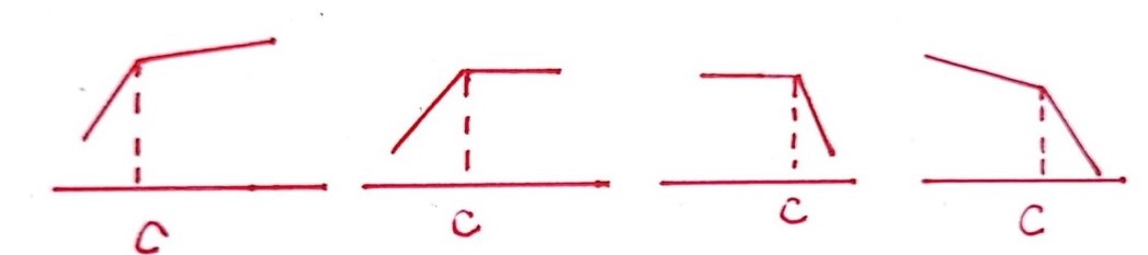
Figure 1. Ridges

3.3. Decay estimates under Von Mises coordinates

Proposition 3.6.

For any fixed $\alpha\in(0,1),$ there exist positive constants $C_{B}$, $B$ and $N$ large and a small positive constant $\lambda>0$ such that

$$|\phi(x,\psi)|\leq g(x,\psi)e^{-B(x+1)^{-\frac{\lambda}{2}}}\quad\text{in}\quad\mathbf{R}_{+}\times\mathbf{R}_{+},$$

where

$$g(x,\psi)=C_{B}\left\{\begin{aligned} N^{1-\alpha}(x+1)^{-\frac{1}{2}-\frac{1-\alpha}{2}}\psi^{1-\alpha},&\quad h<\frac{1}{N},\\ \frac{1}{b_{0}}\partial_{\psi}\bar{w},&\quad h\geq\frac{1}{N},\end{aligned}\right.$$

with $b_{0}=2f^{\prime\prime}(\zeta_{0})$ and $f(\zeta_{0})=\frac{1}{N}.$

Remark 3.7.

At $h=\frac{1}{N}$, $\partial_{\psi}\bar{w}(x,\psi)=\frac{2}{\sqrt{x+1}}f^{\prime\prime}(\zeta_{0}).$ Hence, $g$ is continuous at $h=\frac{1}{N}$.

Proof.

Note $e^{-B}\leq e^{-B(x+1)^{-\frac{\lambda}{2}}}\leq 1.$ Take $C_{B}\in(e^{B},+\infty)$ to be a large constant such that by (3.6), (2.5) and (2.11),

$$(ge^{-B(x+1)^{-\frac{\lambda}{2}}}\pm\phi)(0,\psi)\geq 0.$$

On the other hand, by (1.5), (3.5) and (2.11), we have

$$(ge^{-B(x+1)^{-\frac{\lambda}{2}}}\pm\phi)(x,0)=0,$$

$$ge^{-B(x+1)^{-\frac{\lambda}{2}}}\pm\phi\rightarrow 0\quad\text{as}\,\,h\rightarrow\infty.$$

We claim that $ge^{-B(x+1)^{-\frac{\lambda}{2}}}\pm\phi\geq 0.$ Otherwise, by the initial and boundary conditions above, a negative minimum is obtained at some point $(x_{0},\psi_{0})\in(0,x_{0}]\times(0,+\infty)$ with $(ge^{-B(x+1)^{-\frac{\lambda}{2}}}\pm\phi)(x_{0},\psi_{0})<0$. In the following, we work in the domain $(0,x_{0}]\times(0,+\infty).$

By Lemma 2.2 and (2.11), we have

(3.7) $$C\geq\sqrt{w}\geq c\frac{\psi^{\frac{1}{2}}}{(x+1)^{\frac{1}{4}}},\quad h\leq\frac{1}{2}.$$

By (3.7), in $\{h<\frac{1}{N}\},$ we have

$$Lg=C_{B}N^{1-\alpha}(x+1)^{-\frac{1}{2}-\frac{1-\alpha}{2}-1}\psi^{1-\alpha}\Big{(}-\frac{1}{2}-\frac{1-\alpha}{2}+(1-\alpha)\alpha\sqrt{w}\frac{x+1}{\psi^{2}}\Big{)}>0,$$

by taking $N$ large. Note $N$ is independent of choice of $B.$ Then in $\{h<\frac{1}{N}\},$

$$L(ge^{-B(x+1)^{-\frac{\lambda}{2}}})=(Lg)e^{-B(x+1)^{-\frac{\lambda}{2}}}+ge^{-B(x+1)^{-\frac{\lambda}{2}}}B\frac{\lambda}{2}(x+1)^{-\frac{\lambda}{2}-1}>0.$$

Hence, the minimum point $(x_{0},\psi_{0})$ cannot be in $\{h<\frac{1}{N}\}.$

Consider the case of $\{h>\frac{1}{N}\}.$ We first derive the equation for $Lg+Ag.$ Since $g=\frac{C_{B}}{b_{0}}\partial_{\psi}\bar{w}$ for $h>\frac{1}{N},$ a straight calculation gives

$$\partial_{x}g-\sqrt{\bar{w}}\partial_{\psi}^{2}g-\frac{\partial_{\psi}^{2}\bar{w}}{2\sqrt{\bar{w}}}g=0.$$

For the third term, we have

$$-\frac{\partial_{\psi}^{2}\bar{w}}{2\sqrt{\bar{w}}} =-2\frac{\bar{u}_{yy}|_{(x,y(\psi;\bar{u}))}}{\bar{u}|_{(x,y(\psi;\bar{u}))}(\bar{u}|_{(x,y(\psi;\bar{u}))}+u|_{(x,y(\psi;u))})}\frac{\bar{u}|_{(x,y(\psi;\bar{u}))}(\bar{u}|_{(x,y(\psi;\bar{u}))}+u|_{(x,y(\psi;u))})}{2\bar{u}^{2}|_{(x,y(\psi;\bar{u}))}}$$

$$=A\Big{(}1+\frac{\phi}{2\sqrt{\bar{w}}(\sqrt{w}+\sqrt{\bar{w}})}\Big{)}.$$

Hence, we obtain

(3.8) $$\begin{split}&\partial_{x}g-\sqrt{w}\partial_{\psi}^{2}g+Ag\\ &=\frac{\sqrt{w}-\sqrt{\bar{w}}}{\sqrt{\bar{w}}}\Big{(}-A\frac{\phi}{2\sqrt{\bar{w}}(\sqrt{w}+\sqrt{\bar{w}})}g-Ag-\partial_{x}g\Big{)}-A\frac{\phi}{2\sqrt{\bar{w}}(\sqrt{w}+\sqrt{\bar{w}})}g.\end{split}$$

Now we use the properties of $f(\zeta)$ to estimate $\partial_{x}g.$ By (2.14), we have

$$\partial_{\tilde{x}}g|_{(x,\psi)}= \frac{2C_{B}}{b_{0}}\Big{[}\partial_{x}(\frac{1}{\sqrt{x+1}}f^{\prime\prime})+\frac{1}{\sqrt{x+1}}\frac{-\int_{0}^{y}\bar{u}_{x}dy^{\prime}}{\bar{u}}\partial_{y}f^{\prime\prime}\Big{]}|_{\zeta=\frac{y(\psi;\bar{u})}{\sqrt{x+1}}}$$

$$= \frac{2C_{B}}{b_{0}}\Big{[}-\frac{1}{2}\frac{1}{(\sqrt{x+1})^{3}}f^{\prime\prime}-\frac{1}{2}\frac{y}{(\sqrt{x+1})^{4}}f^{\prime\prime\prime}$$

$$+\frac{1}{(\sqrt{x+1})^{2}}\frac{-\int_{0}^{y}-\frac{1}{2}\frac{\bar{y}}{(\sqrt{x+1})^{3}}f^{\prime\prime}d\bar{y}}{\bar{u}}f^{\prime\prime\prime}\Big{]}|_{\zeta=\frac{y(\psi;\bar{u})}{\sqrt{x+1}}}.$$

For the last term,

$$\int_{0}^{y}\frac{\bar{y}}{(\sqrt{x+1})^{3}}f^{\prime\prime}d\bar{y}=\frac{1}{\sqrt{x+1}}\int_{0}^{\zeta}\zeta f^{\prime\prime}d\zeta=\frac{1}{\sqrt{x+1}}(\zeta f^{\prime}(\zeta)-f(\zeta)).$$

Hence, by $f^{\prime\prime\prime}=-\frac{1}{2}ff^{\prime\prime},$

$$\partial_{\tilde{x}}g=-\frac{1}{2(x+1)}g+\frac{1}{4}\frac{1}{x+1}\zeta f(\zeta)g-\frac{1}{4}\frac{1}{x+1}\frac{\zeta f^{\prime}(\zeta)-f(\zeta)}{\bar{u}}f(\zeta)g|_{\zeta=\frac{y(\psi;\bar{u})}{\sqrt{x+1}}},$$

which along with (3.8) gives

$$\partial_{x}g-\sqrt{w}\partial_{\psi}^{2}g+Ag$$

$$=\frac{\sqrt{w}-\sqrt{\bar{w}}}{\sqrt{\bar{w}}}\Big{(}-A\frac{\sqrt{w}-\sqrt{\bar{w}}}{2\sqrt{\bar{w}}}g-Ag\Big{)}-A\frac{\sqrt{w}-\sqrt{\bar{w}}}{2\sqrt{\bar{w}}}g$$

$$\quad-\frac{\sqrt{w}-\sqrt{\bar{w}}}{\sqrt{\bar{w}}}\Big{(}-\frac{1}{2(x+1)}g+\frac{1}{4}\frac{1}{x+1}\zeta f(\zeta)g-\frac{1}{4}\frac{1}{x+1}\frac{\zeta f^{\prime}(\zeta)-f(\zeta)}{\bar{u}}f(\zeta)g\Big{)}|_{(x,y)=(x,y(\psi;\bar{u}))}.$$

Now we estimate $Lg+Ag.$ Thanks to $\sqrt{\bar{w}}\geq c_{0}$ in $\{h>\frac{1}{N}\}$ for some positive constant $c_{0}$ depending on $N$, we infer that

$$|Lg+Ag|\leq C|\sqrt{w}-\sqrt{\bar{w}}|\frac{1}{x+1}g(1+\zeta^{2}+\zeta)|_{(x,y)=(x,y(\psi;\bar{u}))}.$$

Since $|\sqrt{w}-\sqrt{\bar{w}}|<C(x+1)^{-\lambda}$ and $|\sqrt{w}-\sqrt{\bar{w}}|<Ce^{-\zeta^{2}c}$ by Lemma 3.3 and Lemma 3.4, we estimate $Lg+Ag$ in two different regions.

If $\zeta>(x+1)^{\frac{\lambda}{16}},$ we have

$$|Lg+Ag|\leq Ce^{-\zeta^{2}c}\frac{1}{x+1}g(1+\zeta^{2}+\zeta)\leq C\frac{1}{x+1}g\zeta^{-16}\leq gC(x+1)^{-\lambda-1}.$$

If $\zeta\leq(x+1)^{\frac{\lambda}{16}},$ we have

$$|Lg+Ag|\leq C(x+1)^{-\lambda}\frac{1}{x+1}g(1+(x+1)^{\frac{\lambda}{8}})\leq Cg(x+1)^{-\frac{7}{8}\lambda-1}.$$

Finally, we conclude that

$$L(ge^{-B(x+1)^{-\frac{\lambda}{2}}})+Age^{-B(x+1)^{-\frac{\lambda}{2}}}$$

$$=\big{(}Lg+Ag\big{)}e^{-B(x+1)^{-\frac{\lambda}{2}}}+ge^{-B(x+1)^{-\frac{\lambda}{2}}}B\frac{\lambda}{2}(x+1)^{-\frac{\lambda}{2}-1}$$

$$\geq ge^{-B(x+1)^{-\frac{\lambda}{2}}}(-C(x+1)^{-\frac{7}{8}\lambda-1}+B\frac{\lambda}{2}(x+1)^{-\frac{\lambda}{2}-1})>0$$

by taking $B$ large. Hence, in $\{h>\frac{1}{N}\}$,

$$L(ge^{-B(x+1)^{-\frac{\lambda}{2}}}\pm\phi)+A(ge^{-B(x+1)^{-\frac{\lambda}{2}}}\pm\phi)>0.$$

Then the minimum point $(x_{0},\psi_{0})$ cannot be in $\{h>\frac{1}{N}\}.$

On the other hand, the minimum cannot be achieved at the line $\{h=\frac{1}{N}\}$ by (2.9) and $f^{\prime\prime\prime}\leq 0,$ since the graph here is a ridge with respect to $h$ for any fixed $x$. Therefore, there is no negative minimum point $(x_{0},\psi_{0})$ in the interior. ∎

3.4. Proof of Theorem 1.3

Let us first prove the following lemma.

Lemma 3.8.

There exist positive constants $c$ and $C$ such that

$$\Big{|}u(x,y)-\bar{u}\Big{(}x,\int_{0}^{\int_{0}^{y}u(x,y^{\prime})dy^{\prime}}\frac{1}{\sqrt{\bar{w}}(x,\psi^{\prime})}d\psi^{\prime}\Big{)}\Big{|}\leq\frac{C}{\sqrt{x+1}}e^{-c\frac{y^{2}}{x+1}}\quad\text{in}\quad\mathbf{R}_{+}\times\mathbf{R}_{+}.$$

Proof.

For any fixed $(x_{0},y_{0})\in\mathbf{R}_{+}\times\mathbf{R}_{+},$ let $\psi_{0}=\int_{0}^{y_{0}}u(x_{0},y^{\prime})dy^{\prime}.$ Then we have

$$u(x_{0},y_{0})=\sqrt{w}(x_{0},\psi_{0}),\quad\bar{u}\Big{(}x_{0},\int_{0}^{\int_{0}^{y_{0}}u(x_{0},y^{\prime})dy^{\prime}}\frac{1}{\sqrt{\bar{w}}(x_{0},\psi^{\prime})}d\psi^{\prime}\Big{)}=\sqrt{\bar{w}}(x_{0},\psi_{0}).$$

Since $cy(\psi;\bar{u})\leq y(\psi;u)\leq Cy(\psi;\bar{u}),$ it suffices to show that

$$|\sqrt{w}(x,\psi)-\sqrt{\bar{w}}(x,\psi)|\leq\frac{C}{\sqrt{x+1}}e^{-c\frac{(y(\psi;u))^{2}}{x+1}}\quad\text{in}\quad\mathbf{R}_{+}\times\mathbf{R}_{+}.$$

By (3.5) and Proposition 3.6, we have

$$|\phi(x,\psi)|\leq C\frac{1}{\sqrt{x+1}}h^{\frac{3}{4}}\quad\text{for}\,\,h<1,$$

$$|\phi(x,\psi)|\leq C\frac{1}{\sqrt{x+1}}e^{-c\zeta^{2}}\quad\text{for}\,\,h\geq 1.$$

Note that in $\{h\leq 1\},$ $\sqrt{w}(x,\psi)\sim\sqrt{\bar{w}}(x,\psi)\sim h^{\frac{1}{2}}$ and in $\{h\geq 1\},$ $\sqrt{w}\sim\sqrt{\bar{w}}\geq a_{0}$ for some positive constant $a_{0}$. Then we derive our result from $\sqrt{w}-\sqrt{\bar{w}}=\frac{\phi}{\sqrt{w}+\sqrt{\bar{w}}}$.∎

Now we prove Theorem 1.3.

Proof.

By Lemma 3.8, we have

$$\begin{split}|u(x,y)-\bar{u}(x,y)|&\leq|u(x,y)-\bar{u}(x,\bar{y})|+|\bar{u}(x,\bar{y})-\bar{u}(x,y)|\\ &\leq\frac{C}{\sqrt{x+1}}e^{-c\frac{y^{2}}{x+1}}+|\partial_{\bar{y}}\bar{u}(x,\hat{y})||\bar{y}-y|.\end{split}$$

where $\bar{y}=\int_{0}^{\int_{0}^{y}u(x,y^{\prime})dy^{\prime}}\frac{1}{\sqrt{\bar{w}}(x,\psi^{\prime})}d\psi^{\prime}$ and $\hat{y}$ is between $\bar{y}$ and $y$. Thanks to $\int_{0}^{y}u(x,y^{\prime})dy^{\prime}=\int_{0}^{\bar{y}}\bar{u}(x,y^{\prime})dy^{\prime},$ we get by Lemma 2.2 that

$$c\bar{y}\leq y\leq C\bar{y}$$

for some positive constants $c\in(0,1)$ and $C.$ Due to $f^{\prime\prime\prime}\leq 0,$ we have

$$\partial_{y}\bar{u}(x,\hat{y})|\bar{y}-y|\leq\frac{1}{\sqrt{x+1}}f^{\prime\prime}\Big{(}\frac{c\bar{y}}{\sqrt{x+1}}\Big{)}|\bar{y}-y|.$$

Since $0\leq f^{\prime\prime}(s)\leq Ce^{-cs^{2}},$ we only need to show that

(3.9) $$|\bar{y}-y|\leq C+C\ln(x+1)+\frac{Cy}{\sqrt{x+1}}.$$

Fix any $x>0.$ Take $\psi_{1}$ such that $\psi_{1}=\sqrt{x+1}f(1).$

$$|y-\bar{y}|\leq\Big{|}\int_{0}^{\psi_{1}}\frac{1}{\sqrt{w}(x,\psi)}-\frac{1}{\sqrt{\bar{w}}(x,\psi)}d\psi\Big{|}+\Big{|}\int_{\psi_{1}}^{\psi}\frac{1}{\sqrt{w}(x,\psi)}-\frac{1}{\sqrt{\bar{w}}(x,\psi)}d\psi\Big{|},$$

where the second integral should be omitted if $\psi\leq\psi_{1}.$ For the first term, on the one hand,

$$\int_{0}^{\psi_{1}}\frac{1}{\sqrt{w}}-\frac{1}{\sqrt{\bar{w}}}d\psi \leq\int_{0}^{\psi_{1}}\frac{1}{\sqrt{w}}-\frac{1}{\sqrt{\bar{w}}+\frac{1}{\sqrt{x+1}}}d\psi$$

$$\leq\frac{C}{\sqrt{x+1}}\int_{0}^{\psi_{1}}\frac{1}{\sqrt{w}(\sqrt{\bar{w}}+\frac{1}{\sqrt{x+1}})}d\psi$$

$$\leq\frac{C}{\sqrt{x+1}}\int_{0}^{\psi_{1}}\frac{1}{\sqrt{\bar{w}}(\sqrt{\bar{w}}+\frac{1}{\sqrt{x+1}})}d\psi$$

$$\leq C\int_{0}^{1}\frac{1}{\bar{u}+\frac{1}{\sqrt{x+1}}}d\zeta\leq C\int_{0}^{1}\frac{1}{b\zeta+\frac{1}{\sqrt{x+1}}}d\zeta$$

$$\leq C+C\ln\sqrt{x+1},$$

where we used $f^{\prime\prime}(\zeta)\geq b>0,\,\zeta\leq 1,$ Lemma 2.2, $d\psi=\sqrt{x+1}f^{\prime}(\zeta)d\zeta$ implying $\frac{d\psi}{\sqrt{x+1}\sqrt{\bar{w}}}=d\zeta$; on the other hand,

$$\int_{0}^{\psi_{1}}\frac{1}{\sqrt{\bar{w}}}-\frac{1}{\sqrt{w}}d\psi \leq\int_{0}^{\psi_{1}}\frac{1}{\sqrt{\bar{w}}}-\frac{1}{\sqrt{w}+\frac{5C}{\sqrt{x+1}}}d\psi$$

$$\leq\frac{C}{\sqrt{x+1}}\int_{0}^{\psi_{1}}\frac{1}{\sqrt{\bar{w}}(\sqrt{w}+\frac{5C}{\sqrt{x+1}})}d\psi$$

$$\leq C\int_{0}^{1}\frac{1}{u+\frac{5C}{\sqrt{x+1}}}d\zeta$$

$$\leq C\int_{0}^{1}\frac{1}{b\zeta-\frac{C}{\sqrt{x+1}}+\frac{5C}{\sqrt{x+1}}}d\zeta$$

$$\leq C+C\ln\sqrt{x+1}.$$

For $\psi\geq\psi_{1},$ since $C\geq\sqrt{w}\geq c\sqrt{\bar{w}}\geq cf^{\prime}(1)>0$, we get by Lemma 3.8 that

$$\Big{|}\int_{\psi_{1}}^{\psi}\frac{1}{\sqrt{w}}-\frac{1}{\sqrt{\bar{w}}}d\psi\Big{|}\leq\frac{C}{\sqrt{x+1}}(\psi-\psi_{1})\leq\frac{C}{\sqrt{x+1}}\int_{\psi_{1}}^{\psi}\frac{1}{\sqrt{w}}d\psi\leq\frac{Cy}{\sqrt{x+1}}.$$

This shows (3.9). ∎

4. Decay estimates of $\partial_{x}\phi$ and $\partial_{\psi}^{2}\phi$

In the following sections, we study the Oleinik’s solution $u$ with the initial data satisfying the assumptions in Theorem 1.5.

4.1. Concavity of $u$

Lemma 4.1.

Let $u$ be an Oleinik’s solution with $u_{0}$ satisfying $\partial_{y}^{2}u_{0}\leq 0$. Then it holds that $\partial_{y}^{2}u\leq 0$ in $\mathbf{R}_{+}\times\mathbf{R}_{+}.$

Proof.

Let

$$g=\partial_{x}w=\sqrt{w}\partial^{2}_{\psi}w.$$

By (1.3), we have $g(x,\psi)=\sqrt{w}\partial^{2}_{\psi}w(x,\psi)=2\partial^{2}_{y}u(x,y).$ Thus, we only need to show that

$$g\leq 0\quad\text{in}\quad[0,+\infty)\times\mathbf{R}_{+}.$$

Otherwise, assume that $\sup_{[0,+\infty)\times\mathbf{R}_{+}}g>\epsilon_{0}$ for some $\epsilon_{0}>0$. We define

$$x_{1}=\inf\Big{\{}x^{\prime}\in[0,+\infty)|\exists\psi_{x^{\prime}}\in\mathbf{R}_{+}\,\,\text{so that}\,\,g(x^{\prime},\psi_{x^{\prime}})\geq\frac{\epsilon_{0}}{2}\Big{\}}.$$

Due to $\partial_{y}^{2}u_{0}\leq 0,$ $g|_{x=0}\leq 0$. Hence, $x_{1}\in(0,+\infty).$

In the following, we only consider $g$ in $[0,x_{1}]\times\mathbf{R}_{+}.$ It is easy to see that

$$\partial_{x}g-\frac{g^{2}}{2w}-\sqrt{w}\partial^{2}_{\psi}g=0.$$

Using (1.3), a straight calculation yields

$$\sqrt{w}\partial_{\psi}g(x,\psi)=2u\frac{1}{u}\partial_{y}^{3}u(x,y)=2\partial_{y}^{3}u(x,y).$$

By $|\partial_{y}^{3}u|\leq C$ (See [11] for the bound of $|\partial_{y}^{3}u|$ or see Remark 5.5 in [10]), (2.15) and $g_{+}|_{\psi=0}=0$ due to (2.16), we have

$$\sqrt{w}g_{+}\partial_{\psi}g\rightarrow 0,\quad\text{as}\quad\psi\rightarrow 0\quad\text{and}\quad\text{as}\quad\psi\rightarrow+\infty,$$

$$\frac{\partial_{\psi}w}{2\sqrt{w}}g_{+}^{2}\rightarrow 0\quad\text{as}\,\,\psi\rightarrow 0\quad\text{and}\quad\text{as}\quad\psi\rightarrow+\infty.$$

Then we get by integration by parts that

$$\int_{\mathbf{R}_{+}}\sqrt{w}g_{+}\partial_{\psi}^{2}gd\psi=-\frac{1}{2}\int_{\mathbf{R}_{+}}\partial_{\psi}(\sqrt{w})\partial_{\psi}(g_{+})^{2}d\psi-\int_{\mathbf{R}_{+}}\sqrt{w}(\partial_{\psi}g_{+})^{2}d\psi$$

and

$$-\frac{1}{2}\int_{\mathbf{R}_{+}}\partial_{\psi}(\sqrt{w})\partial_{\psi}(g_{+})^{2}d\psi=\frac{1}{2}\int_{\mathbf{R}_{+}}\partial_{\psi}^{2}(\sqrt{w})(g_{+})^{2}d\psi.$$

In $[0,x_{1}]\times\mathbf{R}_{+},$ we have

$$\partial_{\psi}^{2}(\sqrt{w})=\frac{g}{2w}-\frac{1}{4}\frac{(\partial_{\psi}w)^{2}}{w^{\frac{3}{2}}},\quad\frac{g_{+}^{2}}{2w}g\leq\frac{\epsilon_{0}}{4}\frac{(g_{+})^{2}}{w}.$$

Then we have

(4.1) $$\begin{split}\frac{1}{2}\frac{d}{dx}\int_{\mathbf{R}_{+}}(g_{+})^{2}d\psi+\frac{1}{8}\int_{\mathbf{R}_{+}}\frac{(\partial_{\psi}w)^{2}}{w^{\frac{3}{2}}}(g_{+})^{2}d\psi+\int_{\mathbf{R}_{+}}\sqrt{w}(\partial_{\psi}g_{+})^{2}d\psi\leq C\int_{\mathbf{R}_{+}}\frac{(g_{+})^{2}}{w}d\psi,\end{split}$$

where $C$ depends on $x_{1}.$

By (1.3), there exist some positive constants $c,\,m$ and $M$ so that

$$M>\partial_{\psi}w(x,\psi)>m\quad x\in[0,x_{1}],\,\psi\in[0,c].$$

For any fixed large $K$, by $w|_{\psi=0}=0$, there exists a small positive constant $\psi_{0}<c$ such that for $x\in[0,x_{1}],\psi\in[0,\psi_{0}]$,

$$\frac{(\partial_{\psi}w)^{2}}{w^{\frac{3}{2}}}\geq\frac{m^{2}}{(M)^{\frac{3}{2}}\psi^{\frac{3}{2}}}\geq\frac{K}{m\psi}\geq\frac{K}{w}.$$

On the other hand, by (2.9) and Lemma 2.2, we have

$$w\geq c\bar{w}\geq\tilde{c}_{1}>0\quad\text{on}\quad[\psi_{0},+\infty).$$

Then we have

$$C\int_{0}^{\psi_{0}}\frac{(g_{+})^{2}}{w}d\psi\leq\frac{1}{8}\int_{\mathbf{R}_{+}}\frac{(\partial_{\psi}w)^{2}}{w^{\frac{3}{2}}}(g_{+})^{2}d\psi,$$

$$C\int_{\psi_{0}}^{+\infty}\frac{(g_{+})^{2}}{w}d\psi\leq C\int_{\mathbf{R}_{+}}(g_{+})^{2}d\psi,$$

which along with (4.1) give

(4.2) $$\frac{1}{2}\frac{d}{dx}\int_{\mathbf{R}_{+}}(g_{+})^{2}d\psi\leq C_{x_{1}}\int_{\mathbf{R}_{+}}(g_{+})^{2}d\psi.$$

Since $g_{+}=0$ on $\{x=0\}\times\mathbf{R}_{+}$, by Gronwall’s inequality, we have $g_{+}=0$ in $[0,x_{1}]\times\mathbf{R}_{+},$ which is a contradiction to the definition of $x_{1}$, and thus the proof is completed. ∎

Remark 4.2.

The proof is similar to Proposition 5.4 in [10]. However, a key difference is that we do not require the monotonicity. In particular, we do not require $\partial_{y}u_{0}\geq 0$ in $\mathbf{R}_{+}$.

4.2. Decay estimate of $\phi$ in $\psi$

To obtain a decay estimate of $\partial_{x}\phi,$ we first prove a better decay estimate of $\phi$ with respect to $\psi$ near $0,$ but at the expense of decay rate with respect to $x.$

Lemma 4.3.

There exist positive constants $C,M$ and a small positive constant $\alpha$ such that

$$|\phi(x,\psi)|\leq Cg\quad\text{in}\quad\mathbf{R}_{+}\times\mathbf{R}_{+},$$

where

$$g=C(x+1)^{-\alpha}\left\{\begin{aligned} \frac{1}{b_{1}}\bar{w},&\quad h<\frac{1}{M},\\ 1,&\quad h\geq\frac{1}{M},\end{aligned}\right.$$

with $b_{1}=f^{\prime 2}(\zeta_{0})$ and $\zeta_{0}=f^{-1}(\frac{1}{M}).$

Proof.

By Lemma 2.2, taking $C$ large, we have $\pm\phi\leq g$ on ${x=0}$ and $g=0=\phi$ on $\psi=0.$ By Lemma 3.4, $|\phi|<C(x+1)^{-\alpha}$ for some small $\alpha>0$. Hence, there is no negative minimum of $g\pm\phi$ in $\{h\geq\frac{1}{M}\}.$

Thanks to $\partial_{x}\bar{w}-\sqrt{\bar{w}}\partial^{2}_{\psi}\bar{w}=0,$ we have

$$\partial_{x}\bar{w}-\sqrt{w}\partial^{2}_{\psi}\bar{w}=-(\sqrt{w}-\sqrt{\bar{w}})\partial^{2}_{\psi}\bar{w}=-\frac{\partial_{x}\bar{w}}{\sqrt{\bar{w}}(\sqrt{w}+\sqrt{\bar{w}})}\phi=A\phi,$$

which gives

$$\partial_{x}\bar{w}-\sqrt{w}\partial^{2}_{\psi}\bar{w}+A\bar{w}=A(\bar{w}+\phi)=Aw.$$

Then we get

$$(\partial_{x}-\sqrt{w}\partial^{2}_{\psi})\big{(}(x+1)^{-\alpha}\bar{w}C\big{)}+A(x+1)^{-\alpha}\bar{w}C=(x+1)^{-\alpha}AwC-\alpha(x+1)^{-\alpha-1}\bar{w}C.$$

By (3.1), there exists a positive constant $\lambda_{0}$ such that $A\geq\frac{\lambda_{0}}{x+1}$ for $h\leq 1.$ Therefore, taking $\alpha$ small enough, we obtain

$$(\partial_{x}-\sqrt{w}\partial^{2}_{\psi})(g\pm\phi)+A(g\pm\phi)>0,\,\,0<h<\frac{1}{M}.$$

Hence, there is no negative minimum of $g\pm\phi$ in $\{0<h<\frac{1}{M}\}.$

Since $\partial_{\psi}\bar{w}>0,\,h<\frac{2}{M},$ there is a ridge of $g$ at $h=\frac{1}{M}$ and thus no negative minimum is achieved at $h=\frac{1}{M}$. In summary, $g\pm\phi\geq 0.$ ∎

4.3. The equation of $\partial_{x}\phi=\phi^{1}$

Taking one $x$ derivative of (3.1), we get

(4.3) $$\partial_{x}\phi^{1}-\sqrt{w}\partial_{\psi}^{2}\phi^{1}+A\phi^{1}-\frac{w_{x}}{2w}(\phi^{1}+A\phi)+\phi\partial_{x}A=0.$$

Now we simplify this equation. For this, we use $\partial_{\tilde{x}}$ to denote the derivative in Von Mises coordinates $(\tilde{x},\psi)$ and $\partial_{x}$ for derivatives in Euler coordinates $(x,y)$ in case of confusion. By (3.1) and (2.14), we get

$$\partial_{\tilde{x}}A= \partial_{\tilde{x}}\Big{(}-\frac{\partial_{\tilde{x}}\bar{w}}{\sqrt{\bar{w}}}\frac{1}{\sqrt{\bar{w}}+\sqrt{w}}\Big{)}=\partial_{\tilde{x}}\Big{(}-\frac{\partial_{\tilde{x}}\bar{w}}{\sqrt{\bar{w}}}\Big{)}\frac{1}{\sqrt{\bar{w}}+\sqrt{w}}+\frac{\partial_{\tilde{x}}\bar{w}}{\sqrt{\bar{w}}}\frac{\frac{w_{\tilde{x}}}{2\sqrt{w}}+\frac{\bar{w}_{\tilde{x}}}{2\sqrt{\bar{w}}}}{(\sqrt{w}+\sqrt{\bar{w}})^{2}}$$

$$= \frac{1}{\sqrt{\bar{w}}+\sqrt{w}}\Big{[}\partial_{x}\big{(}-2\frac{\bar{u}_{yy}}{\bar{u}}\big{)}-\frac{\int_{0}^{y}\bar{u}_{x}(x,y^{\prime})dy^{\prime}}{\bar{u}}\partial_{y}\big{(}-2\frac{\bar{u}_{yy}}{\bar{u}}\big{)}\Big{]}|_{(x,y)=(x,y(\psi;\bar{u}))}$$

$$+\frac{w_{\tilde{x}}}{2\sqrt{w}\sqrt{\bar{w}}}\frac{\partial_{\tilde{x}}\bar{w}}{(\sqrt{w}+\sqrt{\bar{w}})^{2}}+\frac{\bar{w}_{\tilde{x}}}{2\bar{w}}\frac{\partial_{\tilde{x}}\bar{w}}{(\sqrt{w}+\sqrt{\bar{w}})^{2}}.$$

We denote

$$D=\partial_{x}\big{(}\frac{\bar{u}_{yy}}{\bar{u}}\big{)}-\frac{\int_{0}^{y}\bar{u}_{x}(x,y^{\prime})dy^{\prime}}{\bar{u}}\partial_{y}\big{(}\frac{\bar{u}_{yy}}{\bar{u}}\big{)}.$$

A direct calculation gives

$$\int_{0}^{y}\bar{u}_{x}(x,y^{\prime})dy^{\prime}= -\frac{1}{2}\frac{1}{(\sqrt{x+1})^{3}}\int_{0}^{y}f^{\prime\prime}(\frac{\tilde{y}}{\sqrt{x+1}})\tilde{y}d\tilde{y}=-\frac{1}{2}\frac{1}{\sqrt{x+1}}\int_{0}^{\zeta}\zeta f^{\prime\prime}(\zeta)d\zeta$$

$$= -\frac{1}{2}\frac{1}{\sqrt{x+1}}(f^{\prime}(\zeta)\zeta-f(\zeta)),$$

$$\frac{\bar{u}_{yy}}{\bar{u}}= \frac{f^{(3)}}{(x+1)f^{\prime}},$$

and then

(4.4) $$\frac{-\int_{0}^{y}\bar{u}_{x}dy^{\prime}}{\bar{u}}=\frac{1}{2}\frac{1}{\sqrt{x+1}}\big{(}\zeta-\frac{f}{f^{\prime}}\big{)}.$$

Thus, we have

$$D= \frac{1}{x+1}\Big{(}\frac{f^{(4)}}{f^{\prime}}-\frac{f^{\prime\prime}f^{(3)}}{(f^{\prime})^{2}}\Big{)}\Big{(}-\frac{y}{2(\sqrt{x+1})^{3}}\Big{)}-\frac{f^{(3)}}{(x+1)^{2}f^{\prime}}$$

$$+\frac{1}{2}\frac{1}{(x+1)^{2}}\Big{(}\zeta-\frac{f}{f^{\prime}}\Big{)}\Big{(}\frac{f^{(4)}}{f^{\prime}}-\frac{f^{\prime\prime}f^{(3)}}{(f^{\prime})^{2}}\Big{)}$$

$$= \frac{1}{(x+1)^{2}}\Big{(}-\frac{1}{2}\frac{f}{f^{\prime}}\Big{)}\Big{(}\frac{f^{(4)}}{f^{\prime}}-\frac{f^{\prime\prime}f^{(3)}}{(f^{\prime})^{2}}\Big{)}-\frac{f^{(3)}}{(x+1)^{2}f^{\prime}}.$$

Further, by (2.3), we have

$$\frac{f^{(4)}}{f^{\prime}}-\frac{f^{\prime\prime}f^{(3)}}{(f^{\prime})^{2}}=-\frac{1}{f^{\prime}}(\frac{1}{2}f^{\prime}f^{\prime\prime}-\frac{1}{4}f^{2}f^{\prime\prime})+\frac{1}{2}\frac{(f^{\prime\prime})^{2}f}{(f^{\prime})^{2}}.$$

This shows that

$$D= \frac{1}{(x+1)^{2}}\Big{[}\big{(}-\frac{1}{2}\frac{f}{f^{\prime}}\big{)}\Big{(}-\frac{1}{f^{\prime}}\big{(}\frac{1}{2}f^{\prime}f^{\prime\prime}-\frac{1}{4}f^{2}f^{\prime\prime}\big{)}+\frac{1}{2}\frac{(f^{\prime\prime})^{2}f}{(f^{\prime})^{2}}\Big{)}+\frac{1}{2}\frac{ff^{\prime\prime}}{f^{\prime}}\Big{]}.$$

By (2.1) and (2.2), for any fixed large $L,$

(4.5) $$D=\frac{1}{(x+1)^{2}}O(\zeta)\,\,\text{for}\,\,\zeta\leq L,\quad D=\frac{1}{(x+1)^{2}}O(f^{\prime\prime}\zeta^{3})\,\,\,\text{for}\,\,\zeta>L,$$

and thus,

(4.6) $$\frac{D}{f^{\prime}}=\frac{1}{(x+1)^{2}}O(1)\,\,\text{for}\,\,\zeta\leq L,\quad\frac{D}{f^{\prime}}=\frac{1}{(x+1)^{2}}O(f^{\prime\prime}\zeta^{3})\,\,\text{for}\,\,\zeta>L.$$

By Proposition 3.6, we get

(4.7) $$|\phi|\leq C(x+1)^{-\frac{1}{2}}f^{\prime\prime}(\zeta)|_{\zeta=\frac{y(\psi;\bar{u})}{\sqrt{x+1}}}\quad\text{for}\,\,h\geq\frac{1}{M},$$

and by Lemma 4.3, for a small positive constant $\alpha,$

(4.8) $$|\phi|=\frac{\bar{w}}{(x+1)^{\alpha}}O(1)\quad\text{for}\,\,h<\frac{1}{M},$$

(4.9) $$\frac{\phi}{(\sqrt{w}+\sqrt{\bar{w}})^{2}}=\frac{1}{(x+1)^{\alpha}}O(1)\quad\text{for}\,\,h<\frac{1}{M}.$$

By Lemma 2.2, we have

(4.10) $$A\phi\sim-\partial_{x}\bar{w}\frac{\phi}{(\sqrt{w}+\sqrt{\bar{w}})^{2}}.$$

Summing up, we conclude that

$$\begin{split}&\partial_{x}\phi^{1}-\sqrt{w}\partial_{\psi}^{2}\phi^{1}+A\phi^{1}-\frac{w_{x}}{2w}\phi^{1}=\frac{w_{x}}{w}O(A\phi)+O(A^{2}\phi)+\phi\frac{D}{f^{\prime}}O(1).\end{split}$$

By (4.7)-(4.10), we have

$$|A\phi|\leq C\frac{-\partial_{x}\bar{w}}{(x+1)^{\alpha}}\leq C\frac{1}{(x+1)^{1+\alpha}}h\quad\text{for}\,\,h<\frac{1}{M},$$

$$|A\phi|\leq C(x+1)^{-\frac{3}{2}}f(f^{\prime\prime})^{2}\leq C(x+1)^{-\frac{3}{2}}\zeta(f^{\prime\prime})^{2}\quad\text{for}\,\,h\geq\frac{1}{M},$$

where we also used $-\partial_{x}\bar{w}=\frac{ff^{\prime\prime}}{x+1},$ $h=f(\zeta)$. By (4.6), (4.7) and (4.8), we get

$$\phi\frac{D}{f^{\prime}}=\frac{\phi}{f^{\prime 2}}\frac{D}{f^{\prime}}(f^{\prime})^{2}=\frac{1}{(x+1)^{2+\alpha}}O(\zeta^{2})\quad\text{for}\,\,\zeta\leq L,$$

$$\phi\frac{D}{f^{\prime}}=(x+1)^{-\frac{5}{2}}O((f^{\prime\prime})^{2}\zeta^{3})\quad\text{for}\,\,\zeta>L.$$

Finally, we arrive at

(4.11) $$\begin{split}&\partial_{x}\phi^{1}-\sqrt{w}\partial_{\psi}^{2}\phi^{1}+A\phi^{1}-\frac{w_{x}}{2w}\phi^{1}=\frac{w_{x}}{w}(D_{4})+D_{5},\end{split}$$

where

$$D_{4}=\frac{1}{(x+1)^{1+\alpha}}O(\zeta^{2})\quad\text{for}\,\,\zeta\leq L,\quad D_{4}=O(\zeta(f^{\prime\prime})^{2})(x+1)^{-\frac{3}{2}}\quad\text{for}\,\,\zeta>L,$$

$$D_{5}=\frac{1}{(x+1)^{2+\alpha}}O(\zeta^{2})\quad\text{for}\,\,\zeta\leq L,\quad D_{5}=(x+1)^{-\frac{5}{2}}O((f^{\prime\prime})^{2}\zeta^{3})\quad\text{for}\,\,\zeta>L.$$

4.4. The equation of $\partial_{x}\bar{w}$

Since $-\partial_{x}\bar{w}$ is useful in constructing barrier functions, here we derive an equation for $\partial_{x}\bar{w}$. Taking one $x$ derivative to $\partial_{x}\bar{w}=\sqrt{\bar{w}}\partial_{\psi}^{2}\bar{w}=2\partial_{y}^{2}\bar{u},$ we obtain

(4.12) $$\partial_{x}(\partial_{x}\bar{w})-\sqrt{\bar{w}}\partial_{\psi}^{2}(\partial_{x}\bar{w})=\frac{(\partial_{x}\bar{w})^{2}}{2\bar{w}}.$$

Thanks to

$$-\frac{\partial_{x}\bar{w}}{2\bar{w}}=A\frac{\sqrt{w}+\sqrt{\bar{w}}}{2\sqrt{\bar{w}}}=A(1+\frac{\phi}{2(\sqrt{w}+\sqrt{\bar{w}})\sqrt{\bar{w}}}),$$

it holds that

$$\partial_{x}(\partial_{x}\bar{w})-\sqrt{w}\partial_{\psi}^{2}(\partial_{x}\bar{w})+\partial_{x}\bar{w}A\Big{(}1+\frac{\phi}{2(\sqrt{w}+\sqrt{\bar{w}})\sqrt{\bar{w}}}\Big{)}$$

$$=-(\sqrt{w}-\sqrt{\bar{w}})\partial_{\psi}^{2}(\partial_{x}\bar{w})$$

$$=-\frac{\phi}{\sqrt{w}+\sqrt{\bar{w}}}\frac{1}{\sqrt{\bar{w}}}\big{(}\partial_{x}(\partial_{x}\bar{w})-\frac{(\partial_{x}\bar{w})^{2}}{2\bar{w}}\big{)}$$

$$=-\frac{\phi}{(\sqrt{w}+\sqrt{\bar{w}})\sqrt{\bar{w}}}\Big{[}\partial_{x}(\partial_{x}\bar{w})+\partial_{x}\bar{w}A\Big{(}1+\frac{\phi}{2(\sqrt{w}+\sqrt{\bar{w}})\sqrt{\bar{w}}}\Big{)}\Big{]}.$$

Due to $\partial_{\tilde{x}}(\frac{\partial_{\tilde{x}}\bar{w}}{2})=\partial_{\tilde{x}}(\partial_{y}^{2}\bar{u})$, we get by (4.4) and (2.14) that

$$\partial_{\tilde{x}}(\partial_{y}^{2}\bar{u})= \partial_{x}\partial_{y}^{2}\bar{u}-\frac{\int_{0}^{y}\bar{u}_{x}dy^{\prime}}{\bar{u}}\partial_{y}\partial_{y}^{2}\bar{u}$$

$$= -\frac{1}{(x+1)^{2}}f^{(3)}+\frac{1}{x+1}\big{(}-\frac{y}{2(\sqrt{x+1})^{3}}\big{)}f^{(4)}+\frac{1}{2}\frac{1}{\sqrt{x+1}}\big{(}\zeta-\frac{f}{f^{\prime}}\big{)}\frac{1}{(\sqrt{x+1})^{3}}f^{(4)}$$

$$= -\frac{1}{(x+1)^{2}}f^{(3)}+\frac{1}{2}\frac{1}{\sqrt{x+1}}\big{(}-\frac{f}{f^{\prime}}\big{)}\frac{1}{(\sqrt{x+1})^{3}}f^{(4)},$$

where we used $\partial_{y}^{2}\bar{u}=\frac{1}{x+1}f^{\prime\prime\prime}.$ Therefore, by the properties of $f$ and (2.3), for large $L$

$$\big{|}\partial_{\tilde{x}}(\frac{\partial_{\tilde{x}}\bar{w}}{2})\big{|}\leq\frac{C}{(x+1)^{2}}\zeta^{2}\quad\text{for}\,\,\zeta\leq L,$$

$$\big{|}\partial_{\tilde{x}}(\frac{\partial_{\tilde{x}}\bar{w}}{2})\big{|}\leq\frac{C}{(x+1)^{2}}f^{\prime\prime}\zeta^{3}\quad\text{for}\,\,\zeta>L.$$

We denote $g_{2}=\partial_{x}\bar{w}$ and $D_{1}=\partial_{x}(\partial_{x}\bar{w})$. Then we find

$$\partial_{x}g_{2}-\sqrt{w}\partial_{\psi}^{2}g_{2}+g_{2}A= -\frac{\phi}{(\sqrt{w}+\sqrt{\bar{w}})\sqrt{\bar{w}}}\Big{[}D_{1}+\partial_{x}\bar{w}A\Big{(}\frac{3}{2}+\frac{\phi}{2(\sqrt{w}+\sqrt{\bar{w}})\sqrt{\bar{w}}}\Big{)}\Big{]}$$

$$= -\frac{\phi}{(\sqrt{w}+\sqrt{\bar{w}})\sqrt{\bar{w}}}(D_{1}+D_{2}).$$

By (4.7) and (4.8), for small positive $\alpha<\frac{1}{2},$

(4.13) $$\begin{split}&\Big{|}\frac{\phi}{(\sqrt{w}+\sqrt{\bar{w}})\sqrt{\bar{w}}}\Big{|}\leq\frac{C}{(x+1)^{\alpha}}\quad\text{for}\,\,\zeta\leq L,\\ &\Big{|}\frac{\phi}{(\sqrt{w}+\sqrt{\bar{w}})\sqrt{\bar{w}}}\Big{|}\leq\frac{Cf^{\prime\prime}}{\sqrt{x+1}}\quad\text{for}\,\,\zeta>L.\end{split}$$

Thanks to $-\partial_{x}\bar{w}A|_{(x,\psi)}\sim\frac{(ff^{\prime\prime}(\zeta))^{2}}{(x+1)^{2}}\frac{1}{(f^{\prime}(\zeta))^{2}},$ by (4.13), we have

$$D_{2} =\frac{1}{(x+1)^{2}}O(\zeta^{2})=\frac{1}{(x+1)^{2}}O(h)\quad\text{for}\,\,\zeta\leq L,$$

$$D_{2} =\frac{1}{(x+1)^{2}}O((f^{\prime\prime})^{2}\zeta^{2})\quad\text{for}\,\,\zeta>L.$$

Let $D_{3}=D_{1}+D_{2}$, which satisfies

(4.14) $$\begin{split}&D_{3}=\frac{1}{(x+1)^{2}}O(\zeta^{2})=\frac{1}{(x+1)^{2}}O(h)\quad\text{for}\,\,\zeta\leq L,\\ &D_{3}=\frac{1}{(x+1)^{2}}O(f^{\prime\prime}\zeta^{3})\quad\text{for}\,\,\zeta>L.\end{split}$$

4.5. Construction of a barrier function

Let $g=(-g_{2})e^{-K(x+1)^{-\epsilon}}.$ Note $g>0$ for $\psi>0.$ By (4.13) and (4.14), we get

$$\begin{split}\partial_{x}&g-\sqrt{w}\partial_{\psi}^{2}g+Ag\geq\epsilon K(x+1)^{-\epsilon-1}(-\partial_{x}\bar{w})e^{-K(x+1)^{-\epsilon}}+e^{-K(x+1)^{-\epsilon}}D_{6}.\end{split}$$

where

$$D_{6}= \frac{1}{(x+1)^{2+\alpha}}O(\zeta^{2})=\frac{1}{(x+1)^{2+\alpha}}O(h)\quad\text{for}\,\,\zeta\leq L,$$

$$D_{6}= \frac{1}{(x+1)^{\frac{5}{2}}}O((f^{\prime\prime})^{2}\zeta^{3})\quad\text{for}\,\,\zeta>L.$$

Thanks to $-\partial_{x}\bar{w}=\frac{1}{x+1}ff^{\prime\prime},$ we have

(4.15) $$-\partial_{x}\bar{w}\sim\frac{1}{x+1}\zeta^{2},\,\,\zeta\leq L,\,\,\,-\partial_{x}\bar{w}\sim\frac{1}{x+1}\zeta f^{\prime\prime},\,\,\zeta>L.$$

Then we infer that

(4.16) $$\begin{split}\partial_{x}&g-\sqrt{w}\partial_{\psi}^{2}g+Ag\geq\frac{1}{2}\epsilon K(x+1)^{-\epsilon-1}(-\partial_{x}\bar{w})e^{-K(x+1)^{-\epsilon}},\end{split}$$

by taking $\epsilon<\alpha$ and $K$ large such that $\epsilon K$ is large.

4.6. Decay estimate of $\partial_{x}\phi$

Proposition 4.4.

There exist positive constants $C_{K}$, $K$ and $\epsilon$ such that

$$|\partial_{x}\phi(x,\psi)|\leq C_{K}g\quad\text{in}\quad\mathbf{R}_{+}\times\mathbf{R}_{+},$$

where $g=(-\partial_{x}\bar{w})e^{-K(x+1)^{-\epsilon}}.$

Proof.

By the assumption, $\partial_{y}u_{0}(0)>0$ and $\partial_{y}^{2}u_{0}(y)=O(y^{2})$ near $y=0$. Then near $\psi=0,$ $|\partial_{x}w|_{x=0}|\leq C\psi.$ On $\{x=0\},$ we have

(4.17) $$\partial_{x}\bar{w}=-\frac{1}{x+1}ff^{\prime\prime}<0\quad\text{for}\,\,\psi>0,$$

(4.18) $$\partial_{x}\bar{w}=-\frac{1}{x+1}ff^{\prime\prime}\sim\psi\quad\psi\,\,near\,\,0.$$

Hence, near $\psi=0,$

(4.19) $$|\partial_{x}\phi|_{x=0}|\leq C\psi\leq C(-\partial_{x}\bar{w}|_{x=0}).$$

By (1.10), (2.2) and (2.7), we have

(4.20) $$|\partial_{x}\phi|_{x=0}|\leq-C\partial_{x}\bar{w}|_{x=0}\quad\text{as}\,\,\psi\rightarrow+\infty.$$

Summing (4.17), (4.19) and (4.20), we deduce that

(4.21) $$|\partial_{x}\phi|_{x=0}|\leq C(-\partial_{x}\bar{w}|_{x=0}).$$

Note $e^{-K}\leq e^{-K(x+1)^{-\epsilon}}\leq 1.$ By (4.21), we may take $C_{K}$ large so that $C_{K}g\pm\phi^{1}(0,\psi)\geq 0$, and $C_{K}g\pm\phi^{1}(x,0)=0$ and $C_{K}g\pm\phi^{1}\rightarrow 0$ as $h\rightarrow\infty.$ Now we claim $C_{K}g\pm\phi^{1}\geq 0.$ Otherwise, a negative minimum is obtained at some point $(x_{0},\psi_{0})\in(0,x_{0}]\times(0,+\infty)$. Let us first point out that $-\frac{w_{x}}{2w}\geq 0.$ By (4.11) and (4.16), in $\{0<h\leq\frac{1}{M}\},$ taking $\epsilon<\alpha$ small, $K\gg\frac{1}{\epsilon}$,

$$\begin{split}&\partial_{x}(C_{K}g\pm\phi^{1})-\sqrt{w}\partial_{\psi}^{2}(C_{K}g\pm\phi^{1})\\ &\qquad+A(C_{K}g\pm\phi^{1})-\frac{w_{x}}{2w}(C_{K}g\pm\phi^{1})\\ &>-\frac{w_{x}}{2w}\Big{[}C_{K}g+\frac{1}{(x+1)^{1+\alpha}}O(\zeta^{2})\Big{]}\\ &\qquad+C_{K}\frac{1}{2}\epsilon K(x+1)^{-\epsilon-1}(-\partial_{x}\bar{w})e^{-K}+\frac{1}{(x+1)^{2+\alpha}}O(\zeta^{2}).\end{split}$$

By (4.15), taking $C_{K}$ large so that $C_{K}\geq Ce^{K}$, we have

$$\partial_{x}(C_{K}g\pm\phi^{1})-\sqrt{w}\partial_{\psi}^{2}(C_{K}g\pm\phi^{1})$$

$$\qquad+A(C_{K}g\pm\phi^{1})-\frac{w_{x}}{2w}(C_{K}g\pm\phi^{1})>0.$$

Therefore, the negative minimum point $(x_{0},\psi_{0})$ cannot be in $\{0<h\leq\frac{1}{M}\}.$

By (4.11) and (4.16), in $\{h\geq\frac{1}{M}\},$ taking $\epsilon<\alpha$ small, $K\gg\frac{1}{\epsilon}$,

(4.22) $$\begin{split}&\partial_{x}(C_{K}g\pm\phi^{1})-\sqrt{w}\partial_{\psi}^{2}(C_{K}g\pm\phi^{1})\\ &\qquad+A(C_{K}g\pm\phi^{1})-\frac{w_{x}}{2w}(C_{K}g\pm\phi^{1})\\ &>-\frac{w_{x}}{2w}\Big{[}C_{K}e^{-K}(-\partial_{x}\bar{w})+O(\zeta(f^{\prime\prime})^{2})(x+1)^{-\frac{3}{2}}\Big{]}\\ &\quad+\frac{1}{2}\epsilon K(x+1)^{-\epsilon-1}C_{K}e^{-K}(-\partial_{x}\bar{w})+(x+1)^{-\frac{5}{2}}O((f^{\prime\prime})^{2}\zeta^{3}).\end{split}$$

By (4.15), taking $C_{K}$ large so that $C_{K}\geq Ce^{K}$, we also have

$$\partial_{x}(C_{K}g\pm\phi^{1})-\sqrt{w}\partial_{\psi}^{2}(C_{K}g\pm\phi^{1})$$

$$\qquad+A(C_{K}g\pm\phi^{1})-\frac{w_{x}}{2w}(C_{K}g\pm\phi^{1})>0.$$

Therefore, the negative minimum point $(x_{0},\psi_{0})$ cannot be in $\{h>\frac{1}{M}\}$. Therefore, there is no negative minimum point $(x_{0},\psi_{0})$ in the interior. ∎

4.7. Proof of Theorem 1.7

By (2.10) and Proposition 3.6, we get

(4.23) $$\begin{split}|\phi(x,\psi)|&\leq\frac{C}{\sqrt{x+1}}e^{-C_{1}\frac{(y(\psi;\bar{u}))^{2}}{x+1}}\leq\frac{C}{\sqrt{x+1}}e^{-c\frac{\psi^{2}}{x+1}}.\end{split}$$

By Lemma 2.2, (2.11) and Proposition 4.4, we have

$$\begin{split}\big{|}\frac{1}{\sqrt{w}}\partial_{x}\phi(x,\psi)\big{|}&\leq|\frac{C}{\sqrt{\bar{w}}}\partial_{x}\phi(x,\psi)|\\ &\leq\frac{C}{x+1}e^{-C_{1}\frac{(y(\psi;\bar{u}))^{2}}{x+1}}\leq\frac{C}{x+1}e^{-c\frac{\psi^{2}}{x+1}}.\end{split}$$

By Lemma 2.2, (2.11) and Proposition 3.6, we have

$$\big{|}\frac{\phi}{\sqrt{w}}(x,\psi)|\leq C|\frac{\phi}{\sqrt{\bar{w}}}(x,\psi)\big{|}\leq\frac{1}{\sqrt{x+1}}e^{-c\frac{\psi^{2}}{x+1}}.$$

By Lemma 3.1, we have

$$\big{|}A\frac{\phi}{\sqrt{w}}(x,\psi)\big{|}\leq\frac{1}{(x+1)^{\frac{3}{2}}}e^{-c\frac{\psi^{2}}{x+1}}.$$

Then we infer from (3.1) that

(4.24) $$\begin{split}|\partial_{\psi}^{2}\phi|&\leq\frac{1}{\sqrt{w}}(|\partial_{x}\phi|+|A\phi|)\\ &\leq\frac{C}{x+1}e^{-c\frac{\psi^{2}}{x+1}}+\frac{1}{(x+1)^{\frac{3}{2}}}e^{-c\frac{\psi^{2}}{x+1}}\leq\frac{C}{x+1}e^{-c\frac{\psi^{2}}{x+1}}.\end{split}$$

Now we prove that

(4.25) $$|\partial_{\psi}\phi|\leq\frac{C}{(x+1)^{\frac{3}{4}}}e^{-c\frac{\psi^{2}}{x+1}}.$$

For any fixed $(x,\psi)\in\mathbf{R}_{+}\times\mathbf{R}_{+}$, take

$$\hat{\psi}=\psi+(x+1)^{\frac{1}{4}}>\psi.$$

Set $\sigma_{x}=(x+1)^{\frac{1}{4}}.$ Then $-\psi+\hat{\psi}=\sigma_{x}.$ By the mean value property, there exists a point $\psi_{1}\in(\psi,\hat{\psi})$ such that

$$\partial_{\psi}\phi(x,\psi_{1})=\frac{\phi(x,\hat{\psi})-\phi(x,\psi)}{\sigma_{x}}.$$

Since $\hat{\psi}>\psi,$ by (4.23),

$$|\partial_{\psi}\phi(x,\psi_{1})|\leq\frac{2\frac{C}{\sqrt{x+1}}e^{-c\frac{\psi^{2}}{x+1}}}{\sigma_{x}}.$$

Then since $\psi_{1}>\psi,$ by (4.24),

$$|\partial_{\psi}\phi(x,\psi)| \leq|\partial_{\psi}\phi(x,\psi)-\partial_{\psi}\phi(x,\psi_{1})|+|\partial_{\psi}\phi(x,\psi_{1})|$$

$$\leq\frac{C}{x+1}e^{-c\frac{\psi^{2}}{x+1}}\sigma_{x}+\frac{\frac{2C}{\sqrt{x+1}}e^{-c\frac{\psi^{2}}{x+1}}}{\sigma_{x}}$$

$$\leq\frac{C}{(x+1)^{\frac{3}{4}}}e^{-c\frac{\psi^{2}}{x+1}}.$$

Since $\psi$ is arbitrarily chosen, we obtain the desired result.

5. Decay estimates of high order derivatives of $w$

In this section, we prove Theorem 1.8.

5.1. Comparison lemma on $\partial_{\psi}w$

Lemma 5.1.

For any $h_{1}>0$, there exists $x_{1}>0$ depending on $h_{1}$ such that

$$\frac{1}{2}\partial_{\psi}\bar{w}\leq\partial_{\psi}w\leq\frac{3}{2}\partial_{\psi}\bar{w}\quad for\,\,h\in[0,h_{1}],\,\,\,\,x\in[x_{1},+\infty).$$

Moreover, $\partial_{\psi}w\geq 0$ in $\mathbf{R}_{+}\times\mathbf{R}_{+}$.

Proof.

By (3.2), we have

$$|A(x,\psi)|\leq\frac{C}{x+1}\frac{-f^{\prime\prime\prime}(\zeta)}{(f^{\prime}(\zeta))^{2}}\leq\frac{C}{x+1}\frac{ff^{\prime\prime}(\zeta)}{(f^{\prime}(\zeta))^{2}}.$$

Hence, by (3.1), Lemma 2.2, Proposition 3.6, Proposition 4.4, (2.12) and the properties of $f$, we deduce that for $h\in[0,h_{1}],$

(5.1) $$\begin{split}|\partial_{\psi}^{2}\phi|&\leq\frac{1}{\sqrt{w}}(|\partial_{x}\phi|+|A\phi|)\\ &\leq\frac{C}{f^{\prime}(\zeta)}\Big{(}(-\partial_{x}\bar{w})+\frac{1}{x+1}\frac{ff^{\prime\prime}(\zeta)}{(f^{\prime}(\zeta))^{2}}\partial_{\psi}\bar{w}\Big{)}\\ &\leq\frac{C}{f^{\prime}(\zeta)}\Big{(}\frac{f(\zeta)}{\sqrt{x+1}}\partial_{\psi}\bar{w}+\frac{1}{x+1}\frac{ff^{\prime\prime}(\zeta)}{(f^{\prime}(\zeta))^{2}}\partial_{\psi}\bar{w}\Big{)}\\ &\leq\frac{C_{h_{1}}}{\sqrt{x+1}}\partial_{\psi}\bar{w},\end{split}$$

where $C_{h_{1}}$ is a positive constant depending on $h_{1}.$

For any fixed $(x,\psi)\in\mathbf{R}_{+}\times\mathbf{R}_{+}$, take

$$\hat{\psi}=\psi+(x+1)^{\frac{1}{4}}>\psi.$$

Set $\sigma_{x}=(x+1)^{\frac{1}{4}}.$ Then $-\psi+\hat{\psi}=\sigma_{x}.$ By the mean value property, there exists a point $\psi_{1}\in(\psi,\hat{\psi})$ such that

$$\partial_{\psi}\phi(x,\psi_{1})=\frac{\phi(x,\hat{\psi})-\phi(x,\psi)}{\sigma_{x}}.$$

Note, by (2.12), $\sqrt{x+1}\partial_{\psi}\bar{w}|_{(x,\psi)}=2f^{\prime\prime}|_{\zeta=\frac{y(\psi;\bar{u})}{\sqrt{x+1}}}$ is decreasing in $h.$ Due to $\hat{\psi}>\psi,$ we get by Proposition 3.6 that

$$|\partial_{\psi}\phi(x,\psi_{1})|\leq\frac{C\partial_{\psi}\bar{w}(x,\psi)}{\sigma_{x}}.$$

Due to $\psi_{1}>\psi,$ we get by (5.1) that

$$|\partial_{\psi}\phi(x,\psi)| \leq|\partial_{\psi}\phi(x,\psi)-\partial_{\psi}\phi(x,\psi_{1})|+|\partial_{\psi}\phi(x,\psi_{1})|$$

$$\leq\sigma_{x}\frac{C_{h_{1}}}{\sqrt{x+1}}\partial_{\psi}\bar{w}(x,\psi)+\frac{C\partial_{\psi}\bar{w}(x,\psi)}{\sigma_{x}}.$$

Then for any $\epsilon\in(0,1),$ we can fix $x_{1}$ large depending on $h_{1}$ and $\epsilon,$ such that

$$(1-\epsilon)\partial_{\psi}\bar{w}\leq\partial_{\psi}w\leq(1+\epsilon)\partial_{\psi}\bar{w},\quad\text{for}\,\,h\in[0,h_{1}]\,\,x\in[x_{1},+\infty).$$

Since $\psi$ is arbitrarily chosen, we obtain the desired result by taking $\epsilon=\frac{1}{2}$.

Since $\partial_{y}^{2}u(x,y)\leq 0$ and the positivity of $u$, $\partial_{y}u$ cannot take a negative value at some point. Then $\partial_{\psi}w\geq 0$ due to $2\partial_{y}u=\partial_{\psi}w$. ∎

5.2. Uniform estimate of $\partial_{x}^{2}\phi$ at a fixed time

Since there is no requirement on higher derivatives of $u_{0}$, we take some positive constant $x_{1}$ as a new initial time and discuss the data on $x=x_{1}.$ Note, by [11], $w$ is smooth in $[x_{1},+\infty)\times(0,+\infty).$

Lemma 5.2.

Under the assumption in Theorem 1.3, for any $x_{1}\in(3,+\infty),$ there exists a constant $c$ independent of $x_{1}$ and two constants $B_{x_{1}}$ and $N_{1}$ depending on $x_{1}$ such that

(5.2) $$|\partial_{x}^{2}\phi(x_{1},\psi)|\leq B_{x_{1}}\left\{\begin{aligned} \frac{1}{N_{1}}e^{-\frac{N_{1}^{2}}{x_{1}+1}c}\psi,\quad&\psi\in[0,N_{1}),\\ e^{-\frac{\psi^{2}}{x_{1}+1}c},\quad&\psi\in[N_{1},+\infty).\end{aligned}\right.$$

Proof.

Let $\phi^{(2)}=\partial_{x}^{2}\phi$. In $D=[x_{1}-2,x_{1}+2]\times[0,+\infty),$ by [11],

(5.3) $$|\phi^{(2)}|\leq|\partial_{x}^{2}w|+|\partial_{x}^{2}\bar{w}|\leq C_{x_{1}}\psi.$$

Hence, we only need to consider in $D_{1}=[x_{1}-2,x_{1}+2]\times[N_{1},+\infty)$ for $N_{1}>3$ large enough determined later.

Firstly, by (4.23), for some positive constants $c_{0}$ and $C$ independent of $x_{1},$

(5.4) $$|\phi|\leq Ce^{-\frac{\psi^{2}}{x+1}c_{0}},\quad\psi\in[\sqrt{x_{1}+2},+\infty),\,\,x\in[x_{1}-2,x_{1}+2].$$

Take $N_{1}$ big enough such that

$$N_{1}>\sqrt{x_{1}+2}+2.$$

For any $\psi_{1}\in[N_{1},+\infty),$ $(x_{2},\psi_{2})\in[x_{1}-1,x_{1}+1]\times[\psi_{1}-1,\psi_{1}+1]$, we consider

$$\partial_{x}(a_{0}\phi)-\sqrt{w}\partial_{\psi}^{2}(a_{0}\phi)+A(a_{0}\phi)=0,\quad A=-\frac{\partial_{x}\bar{w}}{\sqrt{\bar{w}}(\sqrt{\bar{w}}+\sqrt{w})},$$

in $[x_{2}-1,x_{2}+1]\times[\psi_{2}-1,\psi_{2}+1]$, where $a_{0}=e^{\frac{\psi_{2}^{2}}{x_{2}+1}c}$ with $c=\frac{1}{8}c_{0}$ independent of $x_{1}.$ By (5.4), we have

(5.5) $$|a_{0}\phi|\leq|e^{\frac{\psi^{2}}{x+1}c_{0}}\phi|\leq C,$$

where $C$ is independent of $x_{1}.$

Thanks to $w(x,\psi)\rightarrow 1$ and $\bar{w}(x,\psi)\rightarrow 1$ as $\psi\rightarrow+\infty$, for $N_{1}$ big depending on $x_{1},$ we have

(5.6) $$\frac{1}{2}\leq\bar{w},w\leq\frac{3}{2}\quad in\quad D_{1}.$$

Moreover, by [11], we know that any derivative of $w$ has uniform upper and lower bounds $C_{x_{1}}$ and $-C_{x_{1}}$ respectively depending on $x_{1}$ in $D_{1}.$ Then by Schauder estimates in $[x_{2}-1,x_{2}+1]\times[\psi_{2}-1,\psi_{2}+1]$ and (5.5), we have

$$|a_{0}\phi|_{C^{1,\alpha}([x_{2}-\frac{1}{2},x_{2}+\frac{1}{2}]\times[\psi_{2}-\frac{1}{2},\psi_{2}+\frac{1}{2}])}\leq C_{x_{1}}$$

where $C_{x_{1}}$ depends on $x_{1}$ and then

(5.7) $$|a_{0}\phi^{(1)}|_{C^{\alpha}([x_{2}-\frac{1}{2},x_{2}+\frac{1}{2}]\times[\psi_{2}-\frac{1}{2},\psi_{2}+\frac{1}{2}])}\leq C_{x_{1}}.$$

Next we consider the equation of $g=a_{0}\phi^{(1)}$:

$$\begin{split}&\partial_{x}g-\sqrt{w}\partial_{\psi}^{2}g+Ag-\frac{w_{x}}{2w}g+\partial_{x}A\phi a_{0}-\frac{w_{x}}{2w}A(\phi a_{0})=0\end{split}$$

in $\big{[}x_{2}-\frac{1}{2},x_{2}+\frac{1}{2}\big{]}\times\big{[}\psi_{2}-\frac{1}{2},\psi_{2}+\frac{1}{2}\big{]}.$ As before, by the uniform positive upper and lower bounds of $w$ and $\bar{w}$, the bounds of derivatives of $w$ depending on $x_{1}$ and (5.7), we have

$$|g|_{C^{1,\alpha}([x_{2}-\frac{1}{4},x_{2}+\frac{1}{4}]\times[\psi_{2}-\frac{1}{4},\psi_{2}+\frac{1}{4}],)}\leq C_{x_{1}},$$

which gives

$$|\phi^{(2)}|\leq C_{x_{1}}e^{-\frac{\psi_{2}^{2}}{x_{2}+1}c}\quad\text{in}\quad\big{[}x_{2}-\frac{1}{4},x_{2}+\frac{1}{4}\big{]}\times\big{[}\psi_{2}-\frac{1}{4},\psi_{2}+\frac{1}{4}\big{]}.$$

In particular, at $(x_{2},\psi_{2}),$ we have

$$|\phi^{(2)}|\leq C_{x_{1}}e^{-\frac{\psi^{2}}{x+1}c}.$$

Since $(x_{2},\psi_{2})$ is an arbitrary point in $[x_{1}-1,x_{1}+1]\times[\psi_{1}-1,\psi_{1}+1]$ and $\psi_{1}$ is an arbitrary value in $[N_{1},+\infty),$ we conclude that

(5.8) $$|\phi^{(2)}|\leq C_{x_{1}}e^{-\frac{\psi^{2}}{x+1}c}\quad in\quad[x_{1}-1,x_{1}+1]\times[N_{1},+\infty).$$

By restricting (5.8) to $x=x_{1},$ we have the desired result. ∎

5.3. Decay estimate of $\partial_{x}^{2}w$

In this subsection, we discuss under the assumptions in Theorem 1.8. Note, by [11], for any $X>0,$ we can take any order derivative of $w$ in $(0,X)\times(0,+\infty).$

Proposition 5.3.

There exist large positive constants $x_{1},h_{1},B$ and small positive constant $\varepsilon$ such that

(5.9) $$|\partial_{x}^{2}w(x,\psi)|\leq B\big{(}e^{-(x+1)^{-\frac{1}{2}}}\partial_{\psi}w+g)\quad\text{in}\quad[x_{1},+\infty\big{)}\times[0,+\infty),$$

where

$$g(x,\psi)=\frac{1}{(x+1)^{2}}\left\{\begin{aligned} 0,\quad&0\leq h<h_{1}-\frac{3}{2}\pi,\\ \cos(h-h_{1}),\quad&h_{1}-\frac{3}{2}\pi\leq h<h_{1},\\ e^{h_{1}^{2}\varepsilon}e^{-\frac{\psi^{2}}{x+1}\varepsilon},\quad&h\geq h_{1}.\end{aligned}\right.$$

In particular, for any positive constant $h_{2},$ there exist positive constants $x_{2}$ and $B_{2}$ such that

(5.10) $$|\partial_{x}^{2}w(x,\psi)|\leq\frac{B_{2}}{\sqrt{x+1}}\quad\text{in}\,\,h\in[0,h_{2}],\,\,x\in[x_{2},+\infty).$$

Proof.

We first determine $h_{1}$ and $\varepsilon$ which are independent of $x_{1}.$ Let

$$L_{0}v=\partial_{x}v-\sqrt{w}\partial_{\psi}^{2}v,$$

and $h_{1}\in(100,+\infty),\varepsilon\in(0,c)$ where $c$ is the constant independent of $x_{1}$ in Lemma 5.2.

By Lemma 2.2, $w\leq C$ with $C$ independent of $h_{1}$ and $x_{1}$. Taking $\varepsilon$ to be a small positive constant independent of $h_{1}$ and $x_{1}$, we get

$$L_{0}\Big{(}\frac{1}{(x+1)^{2}}e^{-\frac{\psi^{2}}{x+1}\varepsilon}\Big{)} =\frac{1}{(x+1)^{2}}e^{-\frac{\psi^{2}}{x+1}\varepsilon}\Big{[}-\frac{2}{x+1}+\varepsilon\frac{\psi^{2}}{(x+1)^{2}}-\sqrt{w}\Big{(}-\varepsilon\frac{2}{x+1}+\varepsilon^{2}\frac{4\psi^{2}}{(x+1)^{2}}\Big{)}\Big{]}$$

$$\geq\frac{1}{(x+1)^{2}}e^{-\frac{\psi^{2}}{x+1}\varepsilon}\Big{(}-\frac{2}{x+1}+\frac{\varepsilon}{2}\frac{\psi^{2}}{(x+1)^{2}}\Big{)}.$$

This shows that for $h\geq h_{1},$

$$L_{0}\Big{(}\frac{1}{(x+1)^{2}}e^{-\frac{\psi^{2}}{x+1}\varepsilon}\Big{)} \geq\frac{1}{(x+1)^{2}}e^{-\frac{\psi^{2}}{x+1}\varepsilon}\Big{(}-\frac{2}{x+1}+\frac{\varepsilon}{2}\frac{h_{1}^{2}}{x+1}\Big{)}.$$

Fix $h_{1}$ large independent of $x_{1}$ such that $\frac{\varepsilon h_{1}^{2}}{2}>3$ and thus,

(5.11) $$L_{0}g>0\quad\text{for}\,\,h>h_{1}.$$

Next we will determine $x_{1}$ large depending on $h_{1}$ and $B$ large depending on $x_{1}.$ For any $X>x_{1},$ we work in $[x_{1},X]\times[0,+\infty).$ By Lemma 5.2, we have

(5.12) $$\partial_{x}^{2}w=0\quad\text{on}\quad\psi=0,\quad\partial_{x}^{2}w\rightarrow 0\quad\text{as}\quad\psi\rightarrow+\infty,$$

and for $x_{1}$ and $B$ large enough,

$$|\partial_{x}^{2}w|\leq B\big{(}e^{-(x+1)^{-\frac{1}{2}}}\partial_{\psi}w+g\big{)}\quad\text{on}\quad x=x_{1}.$$

Indeed, by Lemma 2.2 and (2.12), for some positive constants $c_{h_{1}}$ and $x_{1}$ depending on $h_{1},$ it holds that for $h\in[0,h_{1}],\,\,x\in[x_{1},+\infty),$

(5.13) $$\begin{split}\partial_{\psi}w(x,\psi)\geq&\frac{1}{2}\partial_{\psi}\bar{w}(x,\psi)\\ \geq&\frac{1}{\sqrt{x+1}}f^{\prime\prime}|_{\zeta=\frac{y(\psi;\bar{u})}{\sqrt{x+1}}}\geq\frac{c_{h_{1}}}{\sqrt{x+1}}.\end{split}$$

Since $|g|\leq\frac{1}{(x+1)^{2}}$ and

(5.14) $$e^{-1}\leq e^{-(x+1)^{-\frac{1}{2}}}\leq 1,$$

we deduce that for $x_{1}$ large depending on $h_{1},$ for some small positive constant $c$ depending on $h_{1},$ it holds

$$e^{-(x+1)^{-\frac{1}{2}}}\partial_{\psi}w+g\geq\frac{c}{\sqrt{x+1}},\quad h\in[0,h_{1}],\,\,x\in[x_{1},+\infty).$$

Then taking $B$ large depending on $x_{1}$ and $h_{1}$, we get by Lemma 5.2 that

(5.15) $$|\partial_{x}^{2}w|\leq B(e^{-(x+1)^{-\frac{1}{2}}}\partial_{\psi}w+g)\quad\text{on}\quad x=x_{1}.$$

Now we work in the interior domain $(x_{1},X]\times(0,+\infty)$. We derive the equations of $F=\partial_{x}^{2}w$ and $\varphi+g$, where $\varphi=e^{-(x+1)^{-\frac{1}{2}}}\partial_{\psi}w.$ Direct calculations show that

$$\partial_{x}F-\sqrt{w}\partial_{\psi}^{2}F-\frac{3\partial_{x}w}{2w}F=-\frac{3(\partial_{x}w)^{3}}{4w^{2}}.$$

Let

$$L_{1}v=\partial_{x}v-\sqrt{w}\partial_{\psi}^{2}v-\frac{3\partial_{x}w}{2w}v.$$

Note $-\frac{3\partial_{x}w}{2w}\geq 0.$ We infer that

(5.16) $$L_{1}(-F)\geq-\frac{3\partial_{x}w}{2w}\Big{(}-\frac{(\partial_{x}w)^{2}}{2w}\Big{)}.$$

From Proposition 4.4, Lemma 2.2 and (2.11), we deduce that for some positive constants $c$ and $C$ independent of $x_{1},$

(5.17) $$\frac{(\partial_{x}w)^{2}}{2w}\leq\frac{C}{(x+1)^{2}}\left\{\begin{aligned} h,\quad&h\leq 1,\\ 1,\quad&1<h\leq 2,\\ e^{-c\frac{\psi^{2}}{x+1}},\quad&2<h.\end{aligned}\right.$$

By a direct calculation, we have

$$\partial_{x}(\partial_{\psi}w)-\sqrt{w}\partial_{\psi}^{2}(\partial_{\psi}w)-\frac{\partial_{x}w}{2w}\partial_{\psi}w=0.$$

Hence, for $\varphi=e^{-(x+1)^{-\frac{1}{2}}}\partial_{\psi}w$, by (5.14), we get

(5.18) $$L_{1}\varphi\geq-\frac{\partial_{x}w}{w}e^{-1}\partial_{\psi}w+\frac{\frac{1}{2}e^{-1}}{(x+1)^{\frac{1}{2}+1}}\partial_{\psi}w\geq 0.$$

Then by (5.11), (5.17) and (5.18), for $B>C$ and $h\in(h_{1},+\infty),$

$$L_{1}\big{(}B(\varphi+g)-F\big{)}>-\frac{3\partial_{x}w}{2w}\Big{(}B\frac{1}{(x+1)^{2}}e^{-\frac{\psi^{2}}{x+1}\varepsilon}-\frac{C}{(x+1)^{2}}e^{-c\frac{\psi^{2}}{x+1}}\Big{)}\geq 0,$$

and thus,

$$L_{1}\big{(}B(\varphi+g)-F\big{)}>0,\quad h>h_{1},$$

where we used $\varepsilon\in(0,c).$

For $h\in(0,h_{1}-\frac{3}{2}\pi),$ by (5.13) and (5.18),

$$L_{1}\big{(}B(\varphi+g)\big{)}>-\frac{3\partial_{x}w}{2w}\frac{2B}{3e}\frac{c_{h_{1}}}{\sqrt{x+1}},$$

where we have used $\partial_{\psi}w>0$ for $h\in(0,h_{1}).$ Hence, by (5.17), for $B$ large depending on $h_{1}$, it holds in $(0,h_{1}-\frac{3}{2}\pi)$ that

$$L_{1}(B(\varphi+g)-F)>0.$$

Next, for $h\in(h_{1}-\frac{3}{2}\pi,h_{1}),$

$$L_{1}g= L_{1}\Big{(}\frac{1}{(x+1)^{2}}\cos\big{(}\frac{\psi}{\sqrt{x+1}}-h_{1}\big{)}\Big{)}\geq-\frac{C_{h_{1}}}{(x+1)^{3}}-\frac{3\partial_{x}w}{2w}(-\frac{1}{(x+1)^{2}})$$

$$\geq -\frac{C_{h_{1}}}{(x+1)^{3}}$$

where $C_{h_{1}}$ is a positive constant depending on $h_{1}.$

Hence, for $h\in(h_{1}-\frac{3}{2}\pi,h_{1}),$ by (5.13) and (5.18) , we have

$$L_{1}(\varphi+g)\geq-\frac{\partial_{x}w}{w}e^{-1}\partial_{\psi}w+\frac{c_{h_{1}}}{(x+1)^{\frac{1}{2}+\frac{3}{2}}}-\frac{C_{h_{1}}}{(x+1)^{3}}.$$

Hence, for $x_{1}$ large depending on $h_{1},$ by (5.13), we have

$$L_{1}\big{(}B(\varphi+g)\big{)}>-\frac{3\partial_{x}w}{2w}\frac{2B}{3e}\frac{c_{h_{1}}}{\sqrt{x+1}},\quad h\in(h_{1}-\frac{3}{2}\pi,h_{1}),\,\,x\in[x_{1},+\infty).$$

Therefore, by (5.17), for $B$ large depending on $h_{1},$ we have

$$L_{1}\big{(}B(\varphi+g)-F\big{)}>0,\quad h\in(h_{1}-\frac{3}{2}\pi,h_{1}),\,\,x\in[x_{1},+\infty).$$

In summary, due to the sign of $L_{1}(Bg-F)$ in $0<h<h_{1}-\frac{3}{2}\pi$, $h_{1}-\frac{3}{2}\pi<h<h_{1}$ and $h>h_{1}$, $-F+B(\varphi+g)$ cannot achieve a negative minimum in $[x_{1},X]\times[0,+\infty)\setminus\{h=h_{1}-\frac{3}{2}\pi,h_{1}\}.$ Moreover, since $h=h_{1}-\frac{3}{2}\pi$ and $h=h_{1}$ are two ridges of $g$, a minimum of $-F+B(\varphi+g)$ cannot be achieved at $h=h_{1}-\frac{3}{2}\pi$ and $h=h_{1}.$ Then we conclude $-F+B(\varphi+g)\geq 0.$

Similarly, we can prove $F+B(\varphi+g)\geq 0$ by following the computations above and using (5.17). ∎

Proposition 5.4.

For any $\alpha\in(0,\frac{1}{8}),$ there exist large positive constants $B,\,h_{1},x_{1}$and small positive constants $h_{0},\varepsilon$ such that

(5.19) $$|\partial_{x}^{2}w(x,\psi)|\leq Bg\quad\text{in}\quad[x_{1},+\infty)\times[0,+\infty),$$

where

$$g(x,\psi)=\frac{1}{(x+1)^{\frac{1}{2}}}\left\{\begin{aligned} h^{1-\alpha},\quad&h\leq h_{0},\\ h_{0}^{1-\alpha},\quad&h_{0}\leq h\leq h_{1},\\ h_{0}^{1-\alpha}e^{h_{1}^{2}\varepsilon}e^{-\frac{\psi^{2}}{x+1}\varepsilon},\quad&h\geq h_{1}.\end{aligned}\right.$$

Proof.

For any $X$ such that $X>x_{1},$ we work in $[x_{1},X]\times[0,+\infty).$ We first determine $h_{0}\in(0,1)$ and $h_{1}.$ By (2.11), we have

$$c\frac{\psi^{\frac{1}{2}}}{(x+1)^{\frac{1}{4}}}\leq\sqrt{w}\leq C\frac{\psi^{\frac{1}{2}}}{(x+1)^{\frac{1}{4}}},\quad h\leq 1,$$

for some constants $c$ and $C$ independent of $x_{1}.$ Hence,

$$L_{0}\Big{(}\frac{\psi^{1-\alpha}}{(x+1)^{\frac{1-\alpha}{2}+\frac{1}{2}}}\Big{)} =\frac{\psi^{1-\alpha}}{(x+1)^{\frac{1-\alpha}{2}+\frac{1}{2}}}\Big{[}-(\frac{1-\alpha}{2}+\frac{1}{2})\frac{1}{x+1}+\sqrt{w}\alpha(1-\alpha)\psi^{-2}\Big{]}$$

$$\geq\frac{\psi^{-1-\alpha}}{(x+1)^{\frac{1-\alpha}{2}+\frac{1}{2}}}[-h^{2}+ch^{\frac{1}{2}}\alpha(1-\alpha)].$$

Hence, we fix $h_{0}$ small depending on $\alpha$ such that

$$L_{0}g>0,\quad 0<h<h_{0}.$$

Therefore, for $B>C$ where $C$ is the constant in (5.17), we get

(5.20) $$L_{1}(Bg)>-\frac{3\partial_{x}w}{2w}\Big{(}\frac{(\partial_{x}w)^{2}}{2w}\Big{)},\quad 0<h<h_{0}.$$

Next we determine $\varepsilon\in(0,c)$ where $c$ is the constant in Lemma 5.2 and then we determine $h_{1}$. Since $w\leq C$ for some positive constant $C$ independent of $h_{1}$ and $x_{1},$ taking $\varepsilon$ to be a small positive constant independent of $h_{1}$ and $x_{1}$, we have

$$L_{0}\Big{(}\frac{1}{\sqrt{x+1}}e^{-\frac{\psi^{2}}{x+1}\varepsilon}\Big{)} =\frac{1}{\sqrt{x+1}}e^{-\frac{\psi^{2}}{x+1}\varepsilon}\Big{[}-\frac{1}{2}\frac{1}{x+1}+\varepsilon\frac{\psi^{2}}{(x+1)^{2}}-\sqrt{w}\Big{(}-\varepsilon\frac{2}{x+1}+\varepsilon^{2}\frac{4\psi^{2}}{(x+1)^{2}}\Big{)}\Big{]}$$

$$\geq\frac{1}{\sqrt{x+1}}e^{-\frac{\psi^{2}}{x+1}\varepsilon}\Big{(}-\frac{1}{2}\frac{1}{x+1}+\frac{\varepsilon}{2}\frac{\psi^{2}}{(x+1)^{2}}\Big{)}.$$

This implies that for $h\geq h_{1},$

$$L_{0}(\frac{1}{\sqrt{x+1}}e^{-\frac{\psi^{2}}{x+1}\varepsilon}) \geq\frac{1}{\sqrt{x+1}}e^{-\frac{\psi^{2}}{x+1}\varepsilon}(-\frac{1}{2}\frac{1}{x+1}+\frac{\varepsilon}{2}\frac{h_{1}^{2}}{x+1}).$$

Fix $h_{1}$ large independent of $x_{1}$ such that $\frac{\varepsilon h_{1}^{2}}{2}>1,$ and thus, $L_{0}g>0$ for $h_{1}<h$. Then by (5.17), for $B$ large depending on $\alpha$ and $h_{0}$, we have

(5.21) $$L_{1}(Bg)>-\frac{3\partial_{x}w}{2w}\big{(}\frac{(\partial_{x}w)^{2}}{2w}\big{)},\quad h>h_{1}.$$

By (5.10), taking $x_{1}$ large depending on $h_{1}$ and $B$ large depending on $h_{1}$ and $h_{0}^{1-\alpha},$ we have

$$|\partial_{x}^{2}w|\leq Bg,\quad h\in[h_{0},h_{1}],\,\,x\in[x_{1},+\infty).$$

Finally, we consider the initial and the boundary data. By Lemma 5.2, we have

(5.22) $$\partial_{x}^{2}w=0\quad on\quad\psi=0,\quad\partial_{x}^{2}w\rightarrow 0\quad as\quad\psi\rightarrow+\infty,\quad|\partial_{x}^{2}w|\leq Cg\quad on\quad x=x_{1},$$

where $C$ is a positive constant depending on $\alpha,h_{1},x_{1},h_{0}$ and $\varepsilon$. Take $B\geq C.$ Then $|\partial_{x}^{2}w|\leq Bg$ on $x=x_{1}$.

Summing up, we have $L_{1}(Bg+F)>0$ in $[x_{1},X]\times[0,+\infty)\setminus\{h=h_{0},h=h_{1}\}$, and thus $\partial_{x}^{2}w+Bg$ cannot achieve a negative minimum in $[x_{1},X]\times[0,+\infty)\setminus\{h=h_{0},h=h_{1}\}.$ Moreover, since $h=h_{0},h=h_{1}$ are two ridges, a minimum of $Bg+F$ cannot be achieved on $h=h_{0}$ and $h=h_{1}$. Then we conclude $Bg+F\geq 0.$

Similarly, we can prove $Bg-F\geq 0.$ ∎

Remark 5.5.

(1) Due to the change of the structure of the equation, a key difficulty in this subsection is how to derive good terms without using the good term $A$ as before. (2) It is necessary to distinguish which terms depend on $x_{1}.$

5.4. Proof of Theorem 1.8

First of all, we infer from Proposition 5.4 that

$$|\partial_{x}^{2}w|\leq\frac{C}{(x+1)^{\frac{1}{2}}}e^{-c\frac{\psi^{2}}{x+1}}.$$

Note that

$$\partial_{x}\partial_{\psi}^{2}w=\partial_{x}(\frac{\partial_{x}w}{\sqrt{w}})=\frac{\partial_{x}^{2}w}{\sqrt{w}}-\frac{1}{2}\frac{(\partial_{x}w)^{2}}{w^{\frac{3}{2}}}.$$

Then by Lemma 2.2, (2.11), Proposition 4.4 and Proposition 5.4, we get

$$|\partial_{x}\partial_{\psi}^{2}w|\leq\frac{C}{(x+1)^{\frac{1}{2}}}e^{-c\frac{\psi^{2}}{x+1}},\quad(x,\psi)\in(N,+\infty)\times(0,+\infty).$$

Following the argument in section 4.7 but taking $\sigma_{x}=(x+1)^{-\frac{1}{4}}$, we can show that

$$|\partial_{\psi x}w|\leq\frac{C}{(x+1)^{\frac{3}{4}}}e^{-c\frac{\psi^{2}}{x+1}},\quad(x,\psi)\in(N,+\infty)\times(0,+\infty).$$

6. Decay estimates of high order derivatives of $u$

In this section, we prove Theorem 1.5, which is a direct consequence of the following Proposition 6.1, Proposition 6.2 and Proposition 6.3.

6.1. Decay estimates of $\partial_{y}u$ and $\partial_{y}^{2}u$

Proposition 6.1.

There exist positive constants $c$ and $C$ such that for any $(x,y)\in\mathbf{R}_{+}\times\mathbf{R}_{+}$,

(6.1) $$-\frac{C}{x+1}e^{-c\frac{y^{2}}{x+1}}\leq\partial_{y}^{2}u(x,y)\leq 0,$$

and

$$|\partial_{y}(u(x,y)-\bar{u}(x,y))|\leq\frac{C}{(x+1)^{\frac{3}{4}}}\ln(x+e)e^{-c\frac{y^{2}}{x+1}}.$$

Proof.

By (1.3), we have

$$2\partial^{2}_{y}u(x,y)=\sqrt{w}\partial^{2}_{\psi}w(x,\psi(x,y))=\partial_{x}w(x,\psi(x,y)),$$

where $\psi(x,y)=\int_{0}^{y}u(x,y^{\prime})dy^{\prime}.$ It follows from Proposition 4.4 that

$$\begin{split}0&\geq\partial_{x}w|_{(x,\psi)}\geq C\partial_{x}\bar{w}|_{(x,\psi)}\\ &\geq-\frac{C}{x+1}ff^{\prime\prime}|_{\zeta=\frac{y(\psi;\bar{u})}{\sqrt{x+1}}}\geq-\frac{C}{x+1}e^{-C_{1}\zeta^{2}}|_{\zeta=\frac{y(\psi;\bar{u})}{\sqrt{x+1}}}\\ &\geq-\frac{C}{x+1}e^{-c\frac{(y(\psi;u))^{2}}{x+1}},\end{split}$$

where we used (2.7). Hence, we have (6.1).

For any fixed $(x,y)\in\mathbf{R}_{+}\times\mathbf{R}_{+}$, take

$$\hat{y}=y+(x+1)^{\frac{1}{4}}>y.$$

Set $\sigma_{x}=(x+1)^{\frac{1}{4}}$ and $\varphi(x,y)=u(x,y)-\bar{u}(x,y).$ Then $-y+\hat{y}=\sigma_{x}.$ By the mean value property, there exists a point $y_{1}\in(y,\hat{y})$ such that

$$\partial_{y}\varphi(x,y_{1})=\frac{\varphi(x,\hat{y})-\varphi(x,y)}{\sigma_{x}}.$$

Since $\hat{y}>y,$ we get by Theorem 1.3 that

$$|\partial_{y}\varphi(x,y_{1})|\leq\frac{2\frac{C}{\sqrt{x+1}}e^{-c\frac{y^{2}}{x+1}}}{\sigma_{x}}\ln(e+x).$$

Then by $y_{1}>y$ and (6.1), we deduce that

$$|\partial_{y}\varphi(x,y)| \leq|\partial_{y}\varphi(x,y)-\partial_{y}\varphi(x,y_{1})|+|\partial_{y}\varphi(x,y_{1})|$$

$$\leq C\frac{1}{x+1}e^{-c\frac{y^{2}}{x+1}}\sigma_{x}+\frac{2\frac{C}{\sqrt{x+1}}e^{-c\frac{y^{2}}{x+1}}}{\sigma_{x}}\ln(x+e)$$

$$\leq C\frac{1}{(x+1)^{\frac{3}{4}}}\ln(x+e)e^{-c\frac{y^{2}}{x+1}}.$$

Since $y$ is arbitrarily chosen, we obtain the desired result. ∎

6.2. Decay estimate of $\partial_{x}u$

Proposition 6.2.

There exist positive constants $c$ and $C$ such that for any $(x,y)\in\mathbf{R}_{+}\times\mathbf{R}_{+}$,

$$|\partial_{x}(u(x,y)-\bar{u}(x,y))|\leq\frac{C}{x+1}e^{-c\frac{y^{2}}{x+1}}.$$

Proof.

We use $\partial_{x}$ to denote the derivative in Euler coordinates $(x,y)$ and $\partial_{\tilde{x}}$ to denote the derivative in Von Mises coordinates $(\tilde{x},\psi).$ We denote

$$h(x,y)=w(x,\psi_{2}(x,y))-\bar{w}(x,\psi_{2}(x,y)),\quad g(x,y)=\bar{w}(x,\psi_{2}(x,y)),$$

where $\psi_{2}(x,y)=\int_{0}^{y}u(x,y^{\prime})dy^{\prime}.$ Here we note, by the composition, the independent variables of both $w(x,\psi_{2}(x,y))$ and $\bar{w}(x,\psi_{2}(x,y))$ are $x$ and $y.$ By the definition of $\psi_{2}(x,y),$ we have

$$w(x,\psi_{2}(x,y))=u(x,y)^{2},$$

and thus,

$$\partial_{x}(u^{2}-\bar{u}^{2})=\partial_{x}h+\partial_{x}(g-\bar{u}^{2}).$$

By a straight computation, we have

$$\partial_{x}h|_{(x,y)}= (\partial_{\tilde{x}}w-\partial_{\tilde{x}}\bar{w})|_{(x,\psi)=(x,\psi_{2}(x,y))}+\partial_{x}\psi_{2}|_{(x,y)}(\partial_{\psi}w-\partial_{\psi}\bar{w})|_{(x,\psi)=(x,\psi_{2}(x,y))},$$

$$\partial_{x}g|_{(x,y)}= \partial_{\tilde{x}}\bar{w}|_{(x,\psi)=(x,\psi_{2}(x,y))}+\partial_{x}\psi_{2}|_{(x,y)}\partial_{\psi}\bar{w}|_{(x,\psi)=(x,\psi_{2}(x,y))},$$

and

$$\partial_{x}(u^{2}-\bar{u}^{2})=2u\partial_{x}u-2\bar{u}\partial_{x}\bar{u}=2u\partial_{x}(u-\bar{u})+2(u-\bar{u})\partial_{x}\bar{u}.$$

Then we obtain

(6.2) $$\begin{split}\partial_{x}(u-\bar{u})|_{(x,y)}=&\frac{1}{2u|_{(x,y)}}\Big{[}\partial_{\tilde{x}}\phi|_{(x,\psi)=(x,\psi_{2}(x,y))}+\partial_{x}\psi_{2}|_{(x,y)}\partial_{\psi}\phi|_{(x,\psi)=(x,\psi_{2}(x,y))}\\ &+\partial_{\tilde{x}}\bar{w}|_{(x,\psi)=(x,\psi_{2}(x,y))}+\partial_{x}\psi_{2}|_{(x,y)}\partial_{\psi}\bar{w}|_{(x,\psi)=(x,\psi_{2}(x,y))}\Big{]}\\ &-\frac{\bar{u}}{u}\partial_{x}\bar{u}|_{(x,y)}-\frac{1}{u}(u-\bar{u})\partial_{x}\bar{u}|_{(x,y)}.\end{split}$$

Now we estimate each term on the right hand side of (6.2). First of all, we show that for some positive constants $c_{9}$ and $C_{9}$,

(6.3) $$c_{9}\bar{u}(x,y)\leq u(x,y)\leq C_{9}\bar{u}(x,y).$$

Since $cy(\psi;\bar{u})\leq y(\psi;u)\leq Cy(\psi;\bar{u})$ and $y(\psi_{2}(x,y);u)=y,$ we get by Lemma 2.2 that

$$u(x,y)= \sqrt{w}(x,\psi_{2}(x,y))$$

$$\leq C\sqrt{\bar{w}}(x,\psi_{2}(x,y))=C\bar{u}(x,y(\psi_{2}(x,y);\bar{u}))$$

$$\leq C\bar{u}(x,Cy(\psi_{2}(x,y);u))=C\bar{u}(x,Cy)\leq C_{9}\bar{u}(x,y),$$

and

$$u(x,y)= \sqrt{w}(x,\psi_{2}(x,y))$$

$$\geq c\sqrt{\bar{w}}(x,\psi_{2}(x,y))=c\bar{u}(x,y(\psi_{2}(x,y);\bar{u}))$$

$$\geq c\bar{u}(x,cy(\psi_{2}(x,y);u))=c\bar{u}(x,cy)\geq c_{9}\bar{u}(x,y).$$

This proves (6.3).

From (6.3) and $\bar{u}(x,y)=f^{\prime}(\frac{y}{\sqrt{x+1}})$, we infer that

$$\frac{1}{u(x,y)}|\partial_{x}\bar{u}(x,y)|\leq\frac{C}{x+1}e^{-c\frac{y^{2}}{x+1}}.$$

By Proposition 4.4, we have

(6.4) $$\begin{split}\frac{1}{u(x,y)}|\partial_{\tilde{x}}\phi|_{(x,\psi)=(x,\psi_{2}(x,y))}|\leq&\frac{C}{f^{\prime}}\frac{ff^{\prime\prime}}{x+1}|_{(x,y)=(x,y(\psi_{2}(x,y);\bar{u}))}\\ \leq&\frac{C}{x+1}e^{-C_{1}\frac{\big{(}y(\psi_{2}(x,y);\bar{u})\big{)}^{2}}{x+1}}\\ \leq&\frac{C}{x+1}e^{-c\frac{\big{(}y(\psi_{2}(x,y);u)\big{)}^{2}}{x+1}}=\frac{C}{x+1}e^{-c\frac{y^{2}}{x+1}}.\end{split}$$

By Lemma 2.2, $d\psi=\sqrt{x+1}f^{\prime}(\zeta)d\zeta$ and Proposition 4.4, we get

$$|\partial_{x}\psi_{2}(x,y)| =\Big{|}\frac{1}{2}\sqrt{w}\int_{0}^{\psi_{2}(x,y)}w^{-\frac{3}{2}}\partial_{\tilde{x}}wd\psi\Big{|}$$

$$\leq C\Big{|}\sqrt{\bar{w}}\int_{0}^{\psi_{2}(x,y)}\bar{w}^{-\frac{3}{2}}\partial_{\tilde{x}}\bar{w}d\psi\Big{|}$$

$$\leq C\sqrt{x+1}f^{\prime}\int_{0}^{\zeta}(f^{\prime})^{-2}\frac{1}{x+1}ff^{\prime\prime}d\tilde{\zeta}|_{\zeta=\frac{y(\psi_{2}(x,y);\bar{u})}{\sqrt{x+1}}}$$

$$\leq\frac{C}{\sqrt{x+1}}e^{-c\frac{(y(\psi_{2}(x,y);\bar{u}))^{2}}{x+1}}$$

$$\leq\frac{C}{\sqrt{x+1}}e^{-c\frac{(y(\psi_{2}(x,y);u))^{2}}{x+1}}=\frac{C}{\sqrt{x+1}}e^{-c\frac{y^{2}}{x+1}}.$$

By (4.25) and (2.10), we get

$$|\partial_{\psi}\phi|_{(x,\psi)=(x,\psi_{2}(x,y))}|\leq\frac{C}{(x+1)^{\frac{3}{4}}}e^{-c\frac{(y(\psi_{2}(x,y);\bar{u}))^{2}}{x+1}}\leq\frac{C}{(x+1)^{\frac{3}{4}}}e^{-c\frac{y^{2}}{x+1}}.$$

Summing up the estimates above and using (2.12), we can conclude our result. ∎

6.3. Decay estimate of $\partial_{x}\partial_{y}u$

Proposition 6.3.

There exist positive constants $c$, $C$ and $N$ such that for any $(x,y)\in(N,+\infty)\times\mathbf{R}_{+}$,

$$|\partial_{xy}u(x,y)|\leq\frac{C}{(x+1)^{\frac{3}{4}}}e^{-c\frac{y^{2}}{x+1}}.$$

Proof.

We use $\partial_{x}$ to denote the derivative in Euler coordinates $(x,y)$ and $\partial_{\tilde{x}}$ to denote the derivative in Von Mises coordinates $(\tilde{x},\psi).$ By (1.3) and (1.4), we get

$$\partial_{x}(2\partial_{y}u) =\partial_{\psi\tilde{x}}w+\partial_{x}\psi\partial_{\psi}^{2}w=\partial_{\psi\tilde{x}}w+\partial_{x}\psi\frac{\partial_{x}w}{\sqrt{w}},$$

$$\partial_{x}\psi =\frac{1}{2}\sqrt{w}\int_{0}^{\psi}w^{-\frac{3}{2}}\partial_{\tilde{x}}wd\psi^{\prime}.$$

From Lemma 2.2, Proposition 4.4 and (2.11), we infer that

$$|\partial_{x}\psi(x,y)| \leq C\Big{|}\int_{0}^{\sqrt{x+1}}w^{-\frac{3}{2}}\partial_{\tilde{x}}wd\psi+\int_{\sqrt{x+1}}^{+\infty}w^{-\frac{3}{2}}\partial_{\tilde{x}}wd\psi\Big{|}$$

$$\leq C\frac{1}{\sqrt{x+1}}\int_{0}^{1}h^{-\frac{3}{2}}hdh+\frac{C}{\sqrt{x+1}}\int_{1}^{+\infty}e^{-ch^{2}}dh$$

$$\leq\frac{C}{\sqrt{x+1}},$$

where we have used (2.12) and $d\psi=\sqrt{x+1}dh.$ Then our result follows from Theorem 1.8 and Proposition 4.4. ∎

References

- [1] A. Dalibard and N. Masmoudi, Separation for the stationary Prandtl equation, Publ. Math. Inst. Hautes Études Sci., 130 (2019), 187-297.
- [2] W. E and B. Engquist, Blowup of solutions of the unsteady Prandtl’s equation, Comm. Pure Appl. Math., 50(1997), 1287-1293.
- [3] Y. Guo and S. Iyer, Validity of steady Prandtl layer expansions, arXiv:1805.05891.
- [4] Y. Guo and S. Iyer, Regularity and expansion for steady Prandtl equations, Comm. Math. Phys., 382 (2021), 1403-1447.
- [5] S. Iyer, On global-in- stability of Blasius profiles, Arch. Rational Mech. Anal., 237(2020), 951-998.
- [6] S. Iyer and N. Masmoudi, Global-in- stability of Steady Prandtl Expansions for 2D Navier-Stokes Flows, arXiv:2008.12347v1.
- [7] I. Kukavica, V. Vicol and F. Wang, The van Dommelen and shen singularity in the Prandtl equtions, Adv. Math., 307(2017), 288-311.
- [8] O. A. Oleinik and V. N. Samokhin, Mathematical models in boundary layer theory, Applied Mathematics and Mathematical Computation 15 Chapman & Hall/CRC, Boca Raton, Fla., 1999.
- [9] J. Serrin, Asymptotic behavior of velocity profiles in the Prandtl boundary layer theory, Proc. R. Soc. Lond. A, 299(1967), 491-507.
- [10] W. Shen, Y. Wang and Z. Zhang, Boundary Layer Separation and Local behavior for the steady Prandtl equation, Adv. Math., 389 (2021), Paper No. 107896.
- [11] Y. Wang and Z. Zhang, Global regularity of the steady Prandtl equation with favorable pressure gradient, Ann. Inst. H. Poincaré Anal. Non Linéaire, https://doi.org/10.1016/j.anihpc.2021.02.007.
- [12] Z. Xin and L. Zhang, On the global existence of solutions to the Prandtl system, Adv. Math., 181(2004), 88-133.