Thermonuclear X-ray bursts from 4U 1636$-$536  observed with AstroSat

Abstract

We report results obtained from the study of 12 thermonuclear X-ray bursts in 6 AstroSat observations of a neutron star X-ray binary and well-known X-ray burster, 4U 1636$-$536. Burst oscillations at $\sim$ 581 Hz are observed with 4–5${\sigma}$ confidence in three of these X-ray bursts. The rising phase burst oscillations show a decreasing trend of the fractional rms amplitude at $3{\sigma}$ confidence, by far the strongest evidence of thermonuclear flame spreading observed with AstroSat. During the initial 0.25 second of the rise a very high value ($34.0\pm 6.7{\%}$) is observed. The concave shape of the fractional amplitude profile provides a strong evidence of latitude-dependent flame speeds, possibly due to the effects of the Coriolis force. We observe decay phase oscillations with amplitudes comparable to that observed during the rising phase, plausibly due to the combined effect of both surface modes as well as the cooling wake. The Doppler shifts due to the rapid rotation of the neutron star might cause hard pulses to precede the soft pulses, resulting in a soft lag. The distance to the source estimated using the PRE bursts is consistent with the known value of $\sim$ 6 kpc.

1 Introduction

Thermonuclear (Type I) X-ray bursts are thought to be sudden eruptions in X-rays due to the unstable burning of hydrogen and helium on the surface of an accreting neutron star in a Low-Mass X-ray Binary (LMXB). Typically, they are characterized by a sharp increase in X-ray intensity and an exponential decay. The burst rise occurs in about 0.5–5 ${\rm{s}}$ while the decline happens in around 10–100 $\rm{s}$ (Lewin, 1977; Hoffman et al., 1978; Lewin et al., 1993; Galloway et al., 2008; Bhattacharyya, 2010). Fast-timing capability of the Rossi X-ray Timing Explorer (RXTE) (Jahoda et al., 2006) led to the discovery of narrow but high-frequency features (mostly in the range: $\sim$ 300–600 Hz) in the power spectrum of these X-ray bursts (see, e.g., Strohmayer et al., 1997a, b). These features are termed as burst oscillations (BOs), either found during their rising/decay phase or in both phases. Thermonuclear X-ray bursts have been observed in more than 100 LMXBs harboring a neutron star, and BOs have been found in quite a few sources (see Bhattacharyya, 2021, and references therein), and there has been a relatively quiet period after the termination of the RXTE mission in 2011. Searching for BOs requires a sensitive instrument, operating in a wide energy band and capable of providing ${\mu}{\rm{s}}$ time resolution. After the launch of AstroSat (Singh et al., 2016) and Neutron Star Interior Composition Explorer (NICER) (Arzoumanian et al., 2014), the hunt for BOs began once again.

Although it is not straightforward to find BOs and constrain their properties, it is important to establish a complete picture of BOs as possible. These are considered to result from the stellar rotation induced modulation of a brightness asymmetry so that pulsations are seen near the spin frequency (see, e.g., Strohmayer et al., 1996; Watts, 2012). Several theories have been proposed to explain these features. Rising phase oscillations are understood due to the flame spreading from the ignition point of the bursts (see, e.g., Strohmayer et al., 1997c) while burst decay oscillations have been explained due to cooling wakes (see, e.g., Mahmoodifar & Strohmayer, 2016, for details). However, none of these explain all the observed BO properties (see the review by Watts, 2012). These features’ frequency can evolve by $1\%$ (of the mean frequency) during a burst, generally from a lower initial value to an asymptotic value (Strohmayer & Bildsten, 2006). In some instances, a downward drift in frequency has also been noted (Strohmayer, 1999; Muno et al., 2000). Energy dependence study of BOs is essential to probe the origin of these features. Attempts have been made in the past to understand phase lags of oscillations (see, e.g., Muno et al., 2003; Artigue et al., 2013). Several possibilities have been discussed in the literature that might be the cause for the soft lag of oscillations (see, e.g., Cui et al., 1998; Ford et al., 1999; Sazonov & Sunyaev, 2001). Explanation for hard lags is a bit challenging though, as it is not clear if hard lags are due to Compton upscattering of photons which should decrease the fractional amplitude at higher energies, but this is in contrast to that observed (Muno et al., 2003). It has also been recently found that different bursts from the same source show a diverse behavior, indicating no lag, hard lag, soft lag or mixed lag (Chakraborty et al., 2017).

Time-resolved spectroscopy during these X-ray bursts have been performed for several sources. The continuum spectra of Type I X-ray bursts is often modelled using an absorbed blackbody, assuming that the entire surface of neutron star emits like a blackbody (see, e.g., Swank et al., 1977; van Paradijs, 1978; Kuulkers et al., 2003). In a conventional method, persistent emission prior to the X-ray burst (also referred to as preburst emission) is assumed to be constant (non-evolving) and subtracted as a background (e.g. Lewin et al., 1993; Bhattacharyya, 2010). Recent studies have found limitations to this assumption, and persistent emission is seen to vary during these X-ray bursts (Worpel et al., 2013, 2015).

There exists a particular class of X-ray bursts called Photospheric Radius Expansion (PRE) burst during which the flux approaches the local Eddington limit causing the photosphere to expand due to radiation pressure (Tawara et al., 1984). A decrease in the blackbody temperature characterizes these bursts while the inferred blackbody radius simultaneously increases. All this happens at an approximately constant value of total flux (see Galloway et al., 2008, for details). When the photosphere returns to the neutron star surface, the temperature has the highest value against a very low blackbody radius value. This stage is called the touchdown (see, e.g., Kuulkers et al., 2003). PRE bursts can be distinguished from typical Type I X-Ray bursts by two maxima in the temperature profile and a burning area maximum corresponding to the temperature minimum (see, e.g., Galloway et al., 2008; Bhattacharyya, 2010). These bursts can serve as distance indicators (see, e.g., Basinska et al., 1984).

In this paper, we report X-ray bursts in 4U 1636$-$536 observed with AstroSat. 4U 1636$-$536 is a neutron star LMXB with an orbital period of $\sim$ 3.8 hr (van Paradijs et al., 1990) and a main-sequence companion star of mass 0.4–0.5 $M_{\odot}$ (Giles et al., 2002; Casares et al., 2006). The distance to the source is $\sim$ 6 kpc (Galloway et al., 2006). The neutron star’s mass is estimated to be 1.6–2.0 $M_{\odot}$ (Casares et al., 2006). 4U 1636$-$536 is classified as an atoll source (Schulz et al., 1989; van der Klis, 1989) based on the track it traces in the color-color diagram (CCD) and the hardness-intensity diagram (HID) (Belloni et al., 2007; Altamirano et al., 2008b) on a $\sim$ 40-day cycle (Shih et al., 2005; Belloni et al., 2007). The transition through CCD or HID is believed to arise from alterations in the mass accretion rate with the source moving from a hard state to a soft state as the accretion rate increases (Bloser et al., 2000; Gierliński & Done, 2002a, b). These two states have different predispositions to different varieties of thermonuclear X-ray bursts (see Hoffman et al., 1977; Galloway et al., 2006; Zhang et al., 2011, for details). As an example, short-recurrence bursts (burst-doublets and burst-triplets) tend to occur during the hard state (e.g., Beri et al., 2019), whereas PRE bursts and superbursts (very long X-ray bursts) as well as BOs are preferentially observed during the soft state (e.g., Güver et al., 2012; Galloway & Keek, 2017). For this source, time-resolved burst spectroscopy has been performed earlier using observations from SAS-3 (Hoffman et al., 1977), Hakucho (Ohashi et al., 1982), EXOSAT (e.g., Turner & Breedon, 1984; Sztajno et al., 1985), RXTE (e.g., Strohmayer et al., 1999; Galloway et al., 2006; Linares et al., 2009; Zhang et al., 2009), Insight-HXMT (Chen et al., 2018) and AstroSat (Beri et al., 2019). Burst oscillations in this source have so far been reported with RXTE data (e.g., Giles et al., 2002) but not with AstroSat data. This paper attempts to fill that gap and we discuss our results in light of proposed theoretical models. Previously, burst oscillation has been reported for a Type I burst in 4U 1728$-$34 using AstroSat observation (Verdhan Chauhan et al., 2017) demonstrating the capability of AstroSat/LAXPC instrument for detecting millisecond variability in these sources.

2 Observations and Data Reduction

2.1 AstroSat/LAXPC

AstroSat is India’s first dedicated multi-wavelength astronomy satellite, launched on September 28, 2015, into a 650 km orbit inclined at an angle of $6\degree$ to the equator by a PSLV C-30 rocket from Satish Dhawan Space Centre (SDSC), SHAR. Its orbital period is 97.6 min (5856 sec). It has five science payloads which cover from X-ray to UV wavelengths (Agrawal, 2006; Paul, 2013; Singh et al., 2016).

Large Area X-ray Proportional Counter (LAXPC) unit consisting of three nominally identical mutually independent detectors labeled as LAXPC10, LAXPC20, and LAXPC30, work in the energy range of 3-80 keV and has an effective collecting area of 6000 cm² in the 5–20 keV band. The LAXPC detectors have a collimator with a field of view of $0.9\degree\times 0.9\degree$. Each detector has 60 anode cells, arranged in 5 layers of 12 cells each, producing 7 anode outputs (2 each from layers 1 & 2, and 1 each from layers 3, 4 & 5) designated A1–A7. The detectors have a time resolution of 10 ${\mu}{\rm{s}}$ and a dead-time of approximately 43 ${\mu}{\rm{s}}$. The energy resolution for LAXPC10, LAXPC20 and LAXPC30 at 30 keV are 15%, 16% and 10% respectively (see §8 of Antia et al., 2017).

It is found that the energy resolution of LAXPC10 is steady while that in LAXPC20 it is degraded from 12 to 16% at 30 keV. On the other hand, the energy resolution of LAXPC30 improved from 11 to 10% (see Antia et al., 2021, for details). In Beri et al. (2019), observations made in February 2016 (just after the launch) were used. Therefore, quoted values of energy resolution are different to those mentioned in this work.

LAXPC data are collected in two different modes: Broad Band Counting (BBC) and Event Analysis mode (EA). The EA mode data contain information about the time, anodeID, and Pulse Height (PHA) of each event, which is why we use this mode of data for timing and spectral analysis. We use the LAXPC software (laxpcsoftv3.0) (Antia et al., 2017) to generate the total spectra, the background spectra and the response files. Since the software applies a suitable dead-time correction to the light curve and spectrum, we do not perform this correction separately. Table 1 gives the log of observations. In this work, we do not include the observation made between 15 and 16 February 2016, reported by Beri et al. (2019), as BOs were not detected during the seven X-ray bursts observed.

Table 1: AstroSat/LAXPC observation details of 4U 1636$-$536. For convenience, we also list which detectors are used in this study for timing (‘T’) and spectral (‘S’) analysis of an observation. ‘X’ indicates ‘omitted’. (see § 2.1)

Observation ID	Observation	Observation	Exposure	Bursts	Burst labels	Used for Analysis
	labels	date	(ks)			LXP10	LXP20	LXP30
G05_195T01_9000000530	Obs 1	2016-07-02	39	2	B1, B2	S, T	S, T	T
G05_195T01_9000000598	Obs 2	2016-08-13	38	1	B3	S, T	S, T	T
G06_104T01_9000001060	Obs 3	2017-02-28	45	2	B4, B5	S, T	S, T	T
G07_040T01_9000001326	Obs 4	2017-06-21	22	3	B6, B7, B8	S, T	S, T	T
G08_033T01_9000002084	Obs 5	2018-05-09	11	2	B9, B10	S, T	S, T	X
G08_033T01_9000002278	Obs 6	2018-08-06	11	2	B11, B12	X	S, T	X

3 Analysis & Results

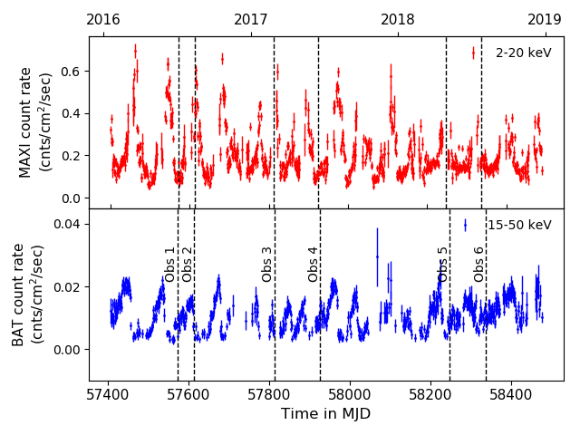
Figure 1: MAXI-GSC and Swift-BAT light curves of 4U 1636$-$536 in 2–20 keV band and 15–50 keV band respectively with vertical dash lines indicating the AstroSat observations used in this work. A signal-to-noise ratio of 3 is used as a filter for both the light curves. (see § 3.1)

3.1 MAXI-GSC and Swift-BAT Light Curves of 4U 1636$-$536

The Swift / Burst Alert Telescope (BAT) is a hard X-ray transient monitor which observes $\sim$ 88% of the sky each day with a detection sensitivity of 5.3 mCrab and a time resolution of 64 seconds, providing almost real-time coverage of the X-ray sky in the energy range 15-50 keV (Krimm et al., 2013). The Gas Slit Camera (GSC: Mihara et al. (2011)) onboard the Monitor of All-sky X-ray Image (MAXI: Matsuoka et al. (2009)) covers $\sim$ 85% of the sky per 92-minute orbital period and $\sim$ 95% per day with a detection sensitivity of 15 mCrab in the 2–20 keV band in a daily scan (Sugizaki et al., 2011).  We use the MAXI and Swift-BAT light curves of 4U 1636$-$536 to determine this source’s spectral state (see Figure 1). The two light curves of 4U 1636$-$536 are binned with a binsize of 1 day. A signal-to-noise ratio of 3 is used as a filter for both the light curves. The peak of the MAXI light curve (high value of flux in 2-20 keV band) indicates a soft spectral state, whereas, the peak of the BAT light curve (high value of flux in 15-50 keV band) suggests a hard spectral state of a source.

3.2 Color-Color Diagram

Atoll sources mainly exhibit three tracks in the color-color diagram, namely, the extreme island state (EIS), the island state (IS) and the banana branch (BB). EIS and IS are spectrally harder states with lower X-ray luminosity whereas BB is the spectrally softer state with higher X-ray luminosity (Altamirano et al., 2008b).

To ascertain the spectral state of the 6 LAXPC observations, we plot the color-color diagram (Figure 2) of all the RXTE observations of 4U 1636$-$536 as given in (Altamirano et al., 2008a) and the location of the observations studied in this paper. For the RXTE observations, hard and soft colors are taken as the 9.7-16.0/6.0-9.7 keV and 3.5-6.0/2.0-3.5 keV count rate ratios, respectively. The colors are normalized by the corresponding Crab Nebula color values that are closest in time to correct for the gain changes as well as for the differences in the effective area between different proportional counters. For the AstroSat observations, only LAXPC20 is used to calculate the color values. The effective area curves for RXTE-PCA and LAXPC are similar in the 3–25 keV range (refer to Figure 1 of Paul (2013)) and we find that the Crab-normalized color values for LAXPC20 are consistent with those reported with RXTE. Therefore, the definition of hard and soft colors is retained as that of RXTE.

The location of the source on the diagram is customarily parametrized by the length of the curve, $S_{a}$. It is normalized so that $S_{a}=1$ at the top-right end and $S_{a}=2$ at the bottom-left end of the diagram (see, e.g. Méndez et al., 1999). $S_{a}$ is believed to represent the mass accretion rate (Hasinger & van der Klis, 1989). From Figure 2, it is clear that Obs 1, Obs 4, Obs 5 and  Obs 6 belong to the hard spectral state while Obs 2 and Obs 3 belong to the soft state of the source.

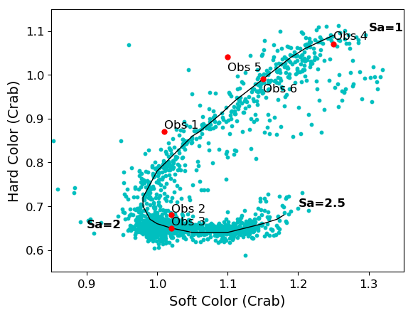
Figure 2: Color-color diagram of 4U 1636$-$536 with positions of the six observations studied in this paper against the RXTE observations (adapted from Altamirano et al., 2008a) shown as cyan dots. The thin solid curve, $S_{a}$, parametrizes the position of the source on the diagram. (see § 3.2)

3.3 Timing Analysis & Results

3.3.1 Energy-Resolved Burst Profile

We find 12 thermonuclear X-ray bursts, and their energy-resolved profiles indicate that all bursts are significantly detected up to 25 keV. To illustrate this, we show here the burst profile of one X-ray burst (see Figure 3). We use five narrow energy bands, viz. 3–6 keV, 6–12 keV, 12–18 keV, 18–24 keV and 24–30 keV. The light curves are created using events from all layers of LAXPC. For the light-curve in the 24–30 keV band, the count-rates are multiplied by a factor of 5 for visual clarity.

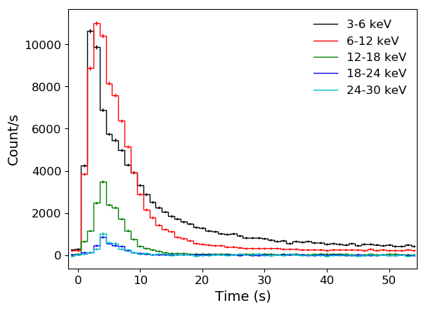
Figure 3: (LAXPC10+LAXPC20+LAXPC30) background-corrected light curve of burst B4. Binsize is 1 s. Count-rates in 24–30 keV band are multiplied by a factor of 5. This figure shows that the X-ray burst is detected up to 30 keV. (see § 3.3.1)

3.3.2 Power Spectrum: Burst Oscillations

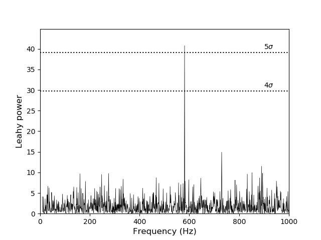
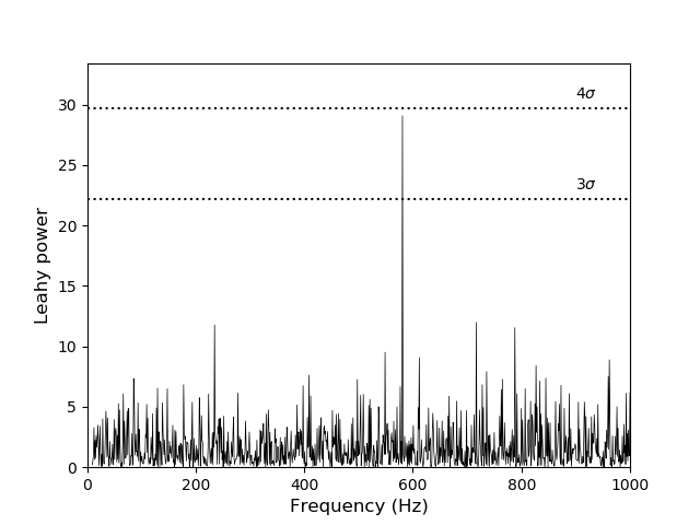
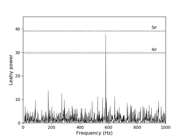
Figure 10: Top Panel: Power spectrum for a 2 s window of burst B3 in Obs 2 in the 8–25 keV band showing burst oscillations at 581 Hz. Middle Panel: Power spectrum for a 3 s window of burst B4 in Obs 3 in the 8–25 keV band showing burst oscillations at 581 Hz. Bottom Panel: Power spectrum for a 1 s window during the rise phase of burst B9 in Obs 5 in the 3–25 keV band showing burst oscillations at 580 Hz. Refer § 3.3.2 for details.

We perform a search for <1024 Hz (Nyquist frequency) oscillations along the entire duration of each of the 12 bursts. Events from all three LAXPC detectors are taken into account, however, LAXPC30 is not used for timing analysis of the two 2018 observations (Obs 5 and Obs 6) owing to its defunct status. The events (photon arrival times) in the 3–25 keV energy band are sampled at the Nyquist rate of 2048 Hz. We perform fast Fourier transform (FFT) of successive 1 s segment (shifting the 1 s time window) of the input barycentre-corrected merged event file corresponding to the burst time interval. The FFT scan is repeated with the start time offset by 0.5 s. A sharp signal at $\sim$ 581 Hz is clearly seen during three of the bursts in the Leahy-normalized (Leahy et al., 1983) power spectrum. In such bursts, we examine the region that shows the signal at $\sim$ 581 Hz and attempt to maximize the measured power, $P_{\text{m}}$, by varying the start and end points of the segment in steps of 0.1 s and trying segment lengths of 1 s, 2 s and 3 s within a time window of 4 s (30+20+10=60 overlapping segments). We also check two more energy bands: 3–8 keV and 8–25 keV. The number of trials is thus, $60\times 3=180$. The single-trial chance probability i.e., the probability of obtaining $P_{\text{m}}$ solely due to noise, is then given by the survival function, $e^{-P_{\text{m}}/2}$, where $P_{\text{m}}$ is now the maximized power obtained through the trials. So, the significance is $x=e^{-P_{\text{m}}/2}\times 180$, and the confidence level would be $X\sigma$, where $X=\sqrt{2}\,\text{erf}^{-1}(1-x)$. The rms fractional amplitude is given by $A=[N_{\gamma}/(N_{\gamma}-N_{\text{bkg}})]\sqrt{P_{\text{s}}/N_{\gamma}}$ (see, e.g., Watts, 2012). $P_{\text{s}}$ is the signal power which can be approximated from $P_{\text{m}}$ using Table 1 (with $k=1$) of Bilous & Watts (2019) if $P_{\text{m}}\gtrsim 2(k+\sqrt{k})$. We use the median value $P_{s}|P_{m}$, so that $P_{s}=P_{m}+1$ and $2\sqrt{P_{m}+1}$ for the uncertainty on $P_{s}$ (see § 4.5 of Bilous & Watts, 2019). $N_{\gamma}$ is the total number of photons, and $N_{\text{bkg}}$ is the number of background photons (estimated from the interval prior to the burst for the same duration and energy range as the FFT window). The results are summarized in Table 1. The power spectra showing $\sim$ 581 Hz are included in Appendix (see Figure 10 in Appendix A).

Table 2: 4U 1636$-$536 burst oscillations as observed with AstroSat/LAXPC. The given values are for the power spectra shown in Figure 10. LAXPC30 was unavailable during burst B9. For details, see § 3.3.2.

Burst	Oscillation	Phase	Chance	Confidence	Fractional
	frequency		probability	level	amplitude
B3	580–581 Hz	decay	$1.38\times 10^{-9}$	$5.2\sigma$	$6.8\pm 1.0$%
B4	580–581 Hz	decay	$4.85\times 10^{-7}$	$3.9\sigma$	$4.6\pm 0.8$%
B9	580–581 Hz	rise	$6.51\times 10^{-9}$	$4.9\sigma$	$13.8\pm 2.2$%

single trial

3.3.3 Energy & Time dependence of BOs

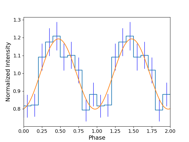
Figure 9: Burst profile as a function of phase, plotted in the 3–25 keV band for a 1 s time window during the rising phase of burst B9. The smooth curve shows the sinusoidal fit with frequency 580.07 Hz. The $\chi_{\nu}^{2}$ (d.o.f.) of the fit is 0.82 (17). The second cycle is shown for clarity. (see § 3.3.3)

To study the energy dependence of $\sim$ 581 Hz oscillations, we model the oscillations with the function $A+B\sin{2\pi\nu t}$ (e.g., see Figure 9 in Appendix A). Here, $B/A$ gives the half-fractional amplitude. The rms fractional amplitude is given by $B/(A\sqrt{2})$, which is comparable to that obtained from the power spectrum. For every time-window that shows oscillation, we determine the best-fit values of A and B, for the frequency which maximizes the fractional amplitude. To check if the oscillation is detected in the chosen window and chosen energy bin, the F-test approach is adopted (see Chakraborty & Bhattacharyya, 2014, for details).

For bursts B3 and B4, the oscillations are mainly seen in the 8–25 keV band, and sparsely in the 3–8 keV band, although a similar number of counts are registered in either band. The variation in rms amplitudes within the 8–25 keV band shows an increasing trend with energy as shown in Figure 4. For B3 and B4, 8–12 keV, 12–16 keV and 16–25 keV bands are used. In the case of burst B9, oscillations are detected in the 3–8 keV band but with strength much less than that in the corresponding 8–25 keV band. An increasing trend in rms amplitudes can be seen from Figure 4 wherein 3–6 keV, 6–8 keV, 8–15 keV and 15–25 keV bands are used for B9. The linear trends have slopes of 0.010, 0.007 and 0.010 keV^-1 for B3, B4 and B9 respectively. Such an increasing trend in the rms amplitude of burst oscillations with energy is typical in non-pulsing systems (see, e.g., Muno et al., 2003).

In Figure 5, we compare the time evolution of fractional amplitude to that of apparent blackbody radius for the decay phase (bursts B3 and B4) and the rising phase (burst B9). The first panel shows the power contours of the dynamic power spectrum of burst rise oscillations superposed on the 0.5 s – binned burst profile. Here we use 2 s windows with new windows starting at 0.25 s intervals. The second panel shows the time evolution of fractional amplitude in 1 s windows; new windows starting at 0.25 s intervals. In case of no detection of oscillation, an upper limit is marked. A range of 3 Hz around the BO frequency is used to search for upper limits. The third panel shows the evolution of the apparent blackbody radius derived from time-resolved spectroscopy.

Next, we study the evolution of the fractional rms amplitude in 3–25 keV during the rise of burst B9. For this, we use 0.25 s binsize for amplitudes since close to the burst onset when the amplitude evolves rapidly, a small time bin is necessary to track the amplitude evolution (Bhattacharyya & Strohmayer, 2007). Rapidly evolving amplitude during the rising phase also implies that the amplitude in a small time bin can be quite high compared to that in a large time bin which averages out the variation. We fit the rms amplitude curve (excluding the upper limits) with an empirical model: $A=a-bc(1-e^{-t/c})$ (Chakraborty & Bhattacharyya, 2014) where $t$ is the time variable, and $a>0$, $b>0$, $c$ are the curve parameters (see Figure 6). The variable $c$ is called the convexity parameter, a positive value of which indicates a concave profile. The curve fitting is performed using curve_fit from the SciPy package. The $\chi_{\nu}^{2}$ (d.o.f.) for the empirical model is 0.78 (5) and $c=0.99\pm 0.52$. We also fit the profile with a constant model and obtain a $\chi_{\nu}^{2}$ (d.o.f.) of 4.27 (7). From the F-test between the two models we find that the empirical model is better than the constant model with a significance of $\approx 3\sigma$, thus emphasizing a decreasing trend. The value of the $c$-parameter implies a concave-shaped time evolution of rising phase rms amplitudes.

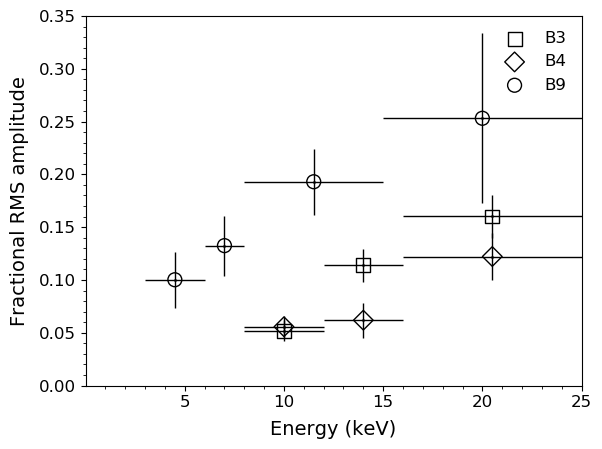
Figure 4: Energy dependence of rms fractional amplitude in a 2 s window during the decay phase of bursts B3 and B4 and in a 1 s window during the rising phase of burst B9. The vertical bars represent $1\sigma$ errors on amplitudes. The horizontal bars show the energy range. (see § 3.3.3)

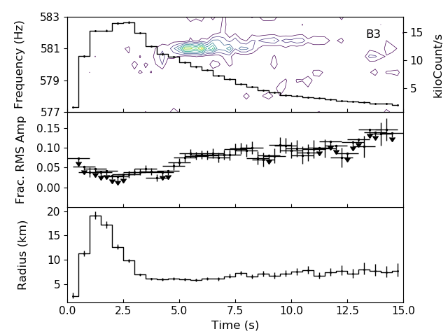
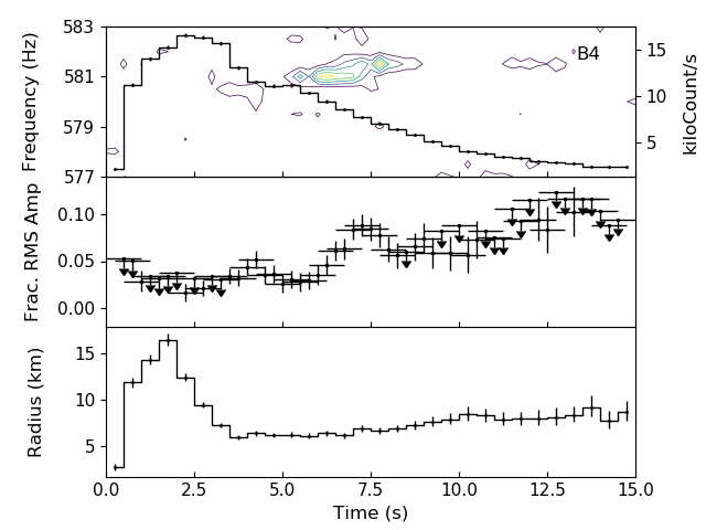
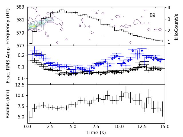
Figure 5: The three plots starting from top are for the three bursts B3, B4 and B9, respectively. DPS and fractional rms amplitudes are drawn in 8–25 keV for bursts B3 and B4, and in 3–25 keV for B9. Amplitudes in 8–25 keV are also shown (in blue) for B9. The contours show Leahy normalized powers starting at 5 (outer contour) and increasing in steps of 5. The down arrow marks the upper limit when oscillation is not detected. Refer § 3.3.3 for details.

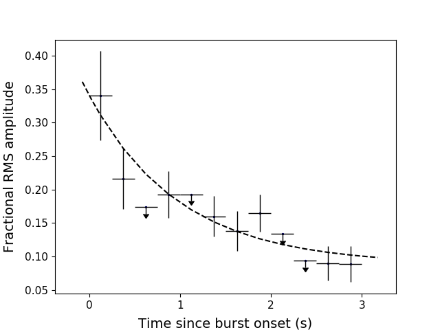
Figure 6: Time evolution of fractional amplitude in 3–25 keV in 0.25 s windows during the rise of burst B9. The vertical bars represent $1\sigma$ errors on amplitudes. The dashed curve shows the best-fit empirical model: $A=a-bc(1-e^{-t/c})$ (Chakraborty & Bhattacharyya, 2014) where $t$ is the time variable, and $a>0$, $b>0$, $c$ are the curve parameters. A positive value of $c$ indicates a concave profile. The best-fit value of c ($=0.99\pm 0.52$) implies latitude-dependent flame speed, possibly due to the effects of the Coriolis force on flame spreading. (see § 3.3.3)

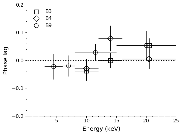
Figure 7: Energy dependence of phase lag of oscillations in a 2 s window during the decay phase of bursts B3 and B4 and in a 1 s window during the rising phase of burst B9. The vertical bars represent $1\sigma$ errors on phase lags. The horizontal bars show the energy range. A positive value of phase lag implies that the pulse in that energy band arrives earlier than the reference band. (see § 3.3.4)

3.3.4 Phase lag of BOs

In Figure 7, we show the energy dependence of the phase lag of the oscillations in the three bursts for the same time windows and energy bands as in Figure 4. A positive slope, in our case, indicates a soft lag. The phase is determined from the folded pulse profiles. The reference phase for calculating phase lag is taken from the folded pulse profile in 8–25 keV band for bursts B3 and B4 and 3–25 keV band for burst B9. Taking respective first bands as reference also gives the same phase lag trends, however, the errors on the phase lag values gets progressively larger for higher bands.

In bursts B3 and B4, we find that the pulse in the lower band (8–12 keV) lags in phase behind the pulse in the upper band (12–16 keV) by 0.04 and 0.11 cycles, respectively, which translate to time delays of 70 and 190 ${\mu}{\rm{s}}$ respectively. In the burst B9 also, the pulse in the lower band (3–8 keV) lags in phase behind the pulse in the upper band (8–15 keV) by 0.05 cycles, equivalent to a time delay of 90 ${\mu}{\rm{s}}$.

3.4 Time-resolved Spectroscopy during X-ray Bursts

3.4.1 Conventional Method

From energy-resolved light curves, we observe that the X-ray bursts are significantly detected up to 25 keV in LAXPC10 and LAXPC20 combined data. Therefore, we use the energy range of 3–25 keV for performing X-ray spectral fitting. Since in LAXPC, the soft and medium energy X-rays hardly reach the bottom layers of the detectors, time-resolved spectroscopy is done using single events from the top layer of each of the two detectors in order to minimize the background (see Beri et al., 2019; Sharma et al., 2020). Data from LAXPC30 are not included for spectral analysis due to its gain instability caused by gas leakage. For Obs 6, LAXPC10 events are also excluded here due to gain loss in LAXPC10 during this observation. 

To study the spectral evolution during X-ray bursts, the spectra during X-ray bursts are extracted for intervals of 0.5 s. For each burst, we also extract the spectrum of 16 s preceding the burst, which is subtracted for all the intervals in the burst as the underlying accretion emission and background. The spectra are grouped using GRPPHA to ensure a minimum of 25 counts per bin. The resulting burst spectra are fitted in XSPEC version 12.10.1f (Arnaud, 1996) using the area normalized blackbody function, ‘BBODYRAD’, which has two variable parameters, viz. color temperature, $T_{\text{bb}}$, and normalization $K_{\text{bb}}=(R_{\text{bb}}/d_{10})^{2}$ where $R_{\text{bb}}$ is the apparent blackbody radius in km, $d_{10}$ is the source distance in units of 10 kpc. In order to model interstellar extinction, the ‘TBABS’ component is used. The photoionization cross sections and elemental abundances of TBABS are specified in Wilms et al. (2000). The only variable parameter in TBABS is $N_{H}$, the Hydrogen column density, which is set to $0.25\times 10^{22}$ cm^-2 (Asai et al., 2000). To account for cross-calibration between LAXPC10 and LAXPC20 (for Obs 1–5), a multiplicative constant component is included in the model. A systematic error of 1% is added while performing the spectral fitting (Antia et al., 2017).

Figure 8 shows the best-fit parameters obtained after performing time-resolved spectroscopy of 3 of the 12 bursts, which evince burst oscillations. The first panel of each plot shows count-rate during the X-ray burst, the second panel shows the temperature evolution, and the third panel shows the blackbody normalization during every 0.5 s segment of the X-ray burst. The radius measured from the values of blackbody normalization is shown in the fourth panel. The unabsorbed bolometric flux (0.1–100 keV), shown in the fifth panel of each plot, is given by (for each time step): $F_{\text{bol}}=\sigma T^{4}(R_{\text{bb}}/d_{10})^{2}=1.0763\times 10^{-11}T_{\text{bb}}^{4}K_{\text{bb}}$ erg cm² s^-1 (Galloway et al., 2006). The sixth panel shows the reduced chi-squared ($\chi_{\nu}^{2}$) obtained from each spectral fitting. The temperature and the radius profile of bursts B3 and B4 suggest that these are PRE bursts. The error bars correspond to 90% confidence.

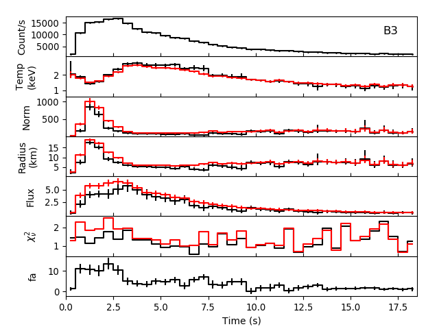
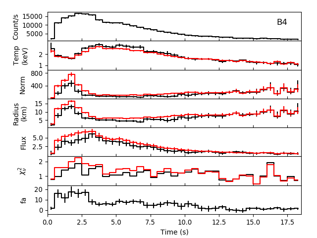
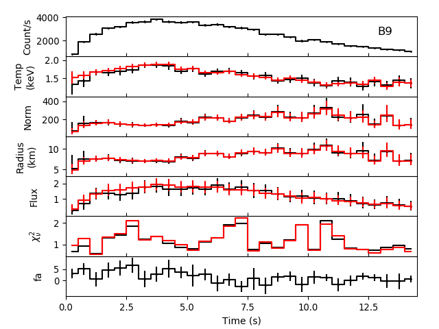
Figure 8: Time-resolved burst profile in 3–25 keV band. Results from conventional method are shown in red, against the results from the $f_{a}$ method. Binsize is 0.5 second. Flux is specified in units of $10^{-8}$ erg cm^-2 s^-1. The three plots starting from top are for the three bursts B3, B4 and B9, respectively. The $f_{a}$ values indicate enhanced persistent emission near the burst peak. Refer § 3.4 for details.

The values of maximum temperature noticed in the PRE bursts B3 and B4 are $2.64\pm 0.05$ keV and $2.68\pm 0.05$ keV, respectively. Other bursts show maximum temperature in the range 1.5–2.4 keV. During the PRE phase, the photospheric radius is found to expand up to $19.1_{-0.7}^{+0.8}$ km in burst B3 and $16.5\pm 0.6$ km in burst B4. Peak fluxes ($F_{\text{max}}$) are $6.71_{-0.65}^{+0.67}$ and $6.82_{-0.64}^{+0.66}$ $\times 10^{-8}$ erg cm^-2 s^-1 for PRE bursts B3 and B4 respectively. These flux values are consistent with the mean $F_{\text{max}}$ of $6.4\pm 0.5$ $\times 10^{-8}$ erg cm^-2 s^-1 for PRE bursts observed by RXTE from 4U 1636$-$536 and using conventional method of spectral fitting (Galloway et al., 2006). For the non-PRE bursts, $F_{\text{max}}$ values lie between 0.6 and 3.6 $\times 10^{-8}$ erg cm^-2 s^-1. $\chi_{\nu}^{2}$ is $\sim$ 1.6–2.3 for the spectra in the PRE phase.

The peak bolometric flux during PRE can be used to estimate the source distance through $d=(L_{\text{Edd}}/4\pi F_{\text{max}})^{1/2}$ (Barrière et al., 2015) where $L_{\text{Edd}}=3.79\pm 0.15\times 10^{38}$ erg s^-1 for H-poor material i.e. $X=0$ (Kuulkers et al., 2003). We obtain a mean source distance of $6.8\pm 0.4$ kpc. However, this $L_{\text{Edd}}$ value is valid only for very large photospheric radius expansion (Galloway et al., 2008). Following Galloway et al. (2020), if we instead use $R=11.2$ km in $1+z(R)$ in Equation 7 of Galloway et al. (2008), we get $L_{\text{Edd}}=2.8\pm 0.1\times 10^{38}$ erg s^-1 for $X=0$ and a source distance estimate of $5.9\pm 0.3$ kpc.

3.4.2 $f_{a}$ method

Worpel et al. (2013, 2015) showed that the persistent emission evolves in the course of the burst as reflected in the dimensionless $f_{a}$ parameter. We apply the $f_{a}$ to both PRE and non-PRE bursts. We use the NTHCOMP model (Zdziarski et al., 1996; Życki et al., 1999) with blackbody seed photons to model the 100 s preburst emission. NTHCOMP is a Comptonization model that is physical and convenient with a small number of parameters. It has two options: the seed photons can result from a single temperature blackbody (e.g., a boundary layer) or from a disk blackbody (e.g., an accretion disk). We choose the first option as it is found to provide a better fit than the second option. For the cases where the electron temperature is not well-constrained in this model, it is fixed to a value of 20 keV. The best fit values (see Table 3) are then fixed as required in the standard $f_{a}$ method and the blackbody model parameters are allowed to vary in the model: ‘TBABS*(BBODYRAD+CONSTANT*NTHCOMP)’. The value of the CONSTANT parameter here is regarded as the $f_{a}$ factor. Figure 8 also shows the results of spectral fitting using the $f_{a}$ method. The bolometric flux for the $f_{a}$ method is calculated as described in § 3.4.1. The evolution of the $f_{a}$ parameter is shown in the last panel.

The maximum temperature observed in a non-PRE burst using the $f_{a}$ method is $2.89^{+0.11}_{-0.10}$ in burst B2. The PRE bursts B3 and B4 show a maximum temperature of $2.75^{+0.09}_{-0.08}$ keV and $2.85^{+0.12}_{-0.11}$ keV, respectively. Other bursts show maximum temperature in the range of 1.5–2.5 keV. The maximum photospheric radius during the PRE phase is calculated to be $17.5_{-1.0}^{+1.1}$ km in burst B3 and $13.0\pm 1.4$ km in burst B4. We find $F_{\text{max}}$ to be $5.79_{-1.15}^{+1.29}$ and $6.03_{-1.16}^{+1.29}$ $\times 10^{-8}$ erg cm^-2 s^-1 for PRE bursts B3 and B4, respectively. For the non-PRE bursts, $F_{\text{max}}$ values range from 0.6 to 3.5 $\times 10^{-8}$ erg cm^-2 s^-1. A considerable overall improvement in the $\chi_{\nu}^{2}$ is found for the PRE bursts showing values in the range $\sim$ 1.1–1.8 while for the non-PRE bursts the $\chi_{\nu}^{2}$ values are comparable to that of the conventional method.

Using the peak flux obtained with this method, the source distance is estimated to be $7.3\pm 0.8$ kpc using $L_{\text{Edd}}=3.79\pm 0.15\times 10^{38}$ erg s^-1. For the alternate case of $L_{\text{Edd}}=2.8\pm 0.1\times 10^{38}$ erg s^-1 mentioned earlier, the estimated distance is $6.3\pm 0.7$ kpc.

Table 3: Fitting NTHCOMP parameters (abbreviated as ‘param.’) for preburst emission of selected bursts (Energy: 3–25 keV; TBABS: $n_{\text{H}}=0.25\times 10^{22}$ cm^-2). “(f)” indicates a “frozen” parameter. $kT_{\text{e}}$ and $kT_{\text{seed}}$ are stated in units of keV. Unabsorbed bolometric persistent flux (0.1–100 keV) is given in units of $10^{-9}$ erg cm^-2 s^-1. For details, see § 3.4.2.

Param.	B3	B4	B9
$\chi^{2}_{\nu}$	1.16	1.02	1.13
d.o.f.	111	114	69
$F_{\text{pers}}$	2.89	2.41	1.43
$\Gamma_{\text{nth}}$	$2.07_{-0.04}^{+0.04}$	$1.85_{-0.04}^{+0.04}$	$1.96_{-0.04}^{+0.04}$
$kT_{\text{e}}$	$3.39_{-0.17}^{+0.19}$	$2.55_{-0.09}^{+0.10}$	20.0 (f)
$kT_{\text{seed}}$	0.51 (f)	0.25 (f)	0.31 (f)
$K_{\text{nth}}$	$0.22_{-0.01}^{+0.01}$	$0.33_{-0.02}^{+0.03}$	$0.11_{-0.01}^{+0.01}$

4 Discussion and Conclusion

In this work, we present spectral and timing analysis of 12 Type I X-ray bursts in 4U 1636$-$536 using the data from AstroSat/LAXPC.

Time-resolved burst spectroscopy is done with 0.5 s time-bin using both the conventional and the $f_{a}$ methods. The evolution of temperature and radius indicates a Photospheric Radius Expansion (PRE) during 2 of these bursts (B3 and B4). The ratio between peak and touchdown radius during PRE burst, the ratio of the temperatures corresponding to the peak radius and the touchdown radius, and similarly for the bolometric fluxes are noted in Table 4. Following the time $R_{\text{bb}}$ reaches its peak value, the flux continues to increase in both the PRE bursts. This was also noted in Sugimoto et al. (1984) for 4U 1636$-$536 and subsequent studies with RXTE (e.g., Galloway et al., 2006). The flux attains its maximum (flux peak) and starts to decrease prior to touchdown. The touchdown phase can be distinguished by high temperature (second maximum in the temperature profile) and a small emitting area. The ratio of $F_{\text{bol}}$ at peak radius and touchdown is lower with the $f_{a}$ method than that with conventional method because of different degree of enhancement of persistent flux (magnitude of $f_{a}$) at the two stages. The (radial) peak to touchdown delay is $\sim$ 2.5 s for PRE burst B3 and $\sim$ 2.0 s for PRE burst B4. The values of peak fluxes and maximum radii for the PRE and the non-PRE bursts given in § 3.4 conform to those reported in Galloway et al. (2006) using RXTE observations of 4U 1636$-$536. Maximum flux, $F_{\text{max}}$, for both the PRE bursts, are higher than that for the non-PRE bursts.

From the spectral analysis using the $f_{a}$ method, we observe that the persistent emission is enhanced near the peak of the burst, especially for the PRE bursts in Obs 2 and Obs 3. The highest value of the $f_{a}$ parameter is seen in the PRE burst B4 to be $17.5\pm 4.9$, whereas in the other PRE burst B3, it is $13.5\pm 2.8$. For the non-PRE bursts, the highest $f_{a}$ value is $\lesssim$10. The $f_{a}$ values are consistent with those provided in Worpel et al. (2013). The flux value in the $f_{a}$ method is lower than that in the conventional method around the peak of the burst since the calculated flux does not include the contribution of the scaled persistent emission to the total flux (Worpel et al., 2013). It should be noted that the maximum $f_{a}$ need not occur at the same moment as the peak radius (Worpel et al., 2013). We find that the two maxima concur in burst B4 but not in burst B3.

As has been observed earlier (e.g., Bhattacharyya et al., 2018), the $f_{a}$ method also gives a lower estimate for the radius as inferred from the blackbody normalization. The ratio of the touchdown radii as determined by the $f_{a}$ and conventional methods (i.e. $R_{\text{TD, }f_{a}}/R_{\text{TD, conv.}}$) is found to be $0.88_{-0.08}^{+0.09}$ and $0.84_{-0.08}^{+0.09}$ for PRE bursts B3 and B4, respectively. These values are comparable to the mean value of $0.97\pm 0.11$ for the touchdown radii ratio obtained in Worpel et al. (2013) with PRE bursts from multiple sources. This difference in touchdown radii estimates poses more challenges to deriving neutron star parameters using radius expansion bursts.

We estimate the source distance using the maximum flux observed during the PRE bursts and obtain a value of $6.8\pm 0.4$ kpc with conventional method which is consistent with the known estimate of $6.0\pm 0.5$ kpc for this source (Galloway et al., 2006). We also calculate the source distance using the assumption as in Galloway et al. (2020) and obtain an estimate of $5.9\pm 0.3$ kpc for the $X=0$ case, in contrast to $5.0\pm 0.5$ kpc as quoted in their paper.

We detect burst oscillations in both the PRE bursts in the post-touchdown (PTD) phase, which corroborates previous findings (Strohmayer et al., 1998; Zhang et al., 2013). The oscillation frequency shows a $\sim$ 1 Hz drift which is consistent with $\lesssim$1% frequency drift observed during Type I X-ray bursts (Strohmayer, 2001; Muno et al., 2002; Watts, 2012). Zhang et al. (2013) found that for PRE bursts in 4U 1636$-$536  a PTD phase of length $\sim$ 2–8 s (long PTD) is an indication of the presence of burst oscillations, where PTD length is defined as the contiguous time interval after the peak during which $R_{\text{bb}}$ remains more or less constant before increasing again. This trend was also noted for PRE bursts in 4U 1728$-$34 (Zhang et al., 2016). The PTD length is $\sim$ 4–5 s for the PRE bursts in this study. Hence, the conjecture of Zhang et al. (2013) holds true in our analysis.

The frequency drift of 1 Hz observed in our analysis can be explained with a simple model based on the conservation of angular momentum. If a 10 m thick layer of accumulated matter expands to about 30 m, then the rotation frequency should decrease by $\delta{\nu}~{}{\approx}~{}2{\nu}(20~{}\text{m}/R)$, where ${\nu}$ and $R$ are the stellar spin frequency and radius, respectively. Therefore, in the beginning of these bursts we observe a burst oscillation frequency which is less than the stellar spin frequency and as the burning layer cools down, its thickness decreases and the burst oscillation frequency increases towards the stellar spin frequency in a few seconds (for more details, see Watts, 2012; Bhattacharyya, 2021). Similar frequency evolution (increase) of burst rise oscillations from 4U 1636$-$536 has also been observed earlier (Bhattacharyya & Strohmayer, 2005). However, this model has certain limitations specifically if the frequency drift is of the order of a few hertz (see Bhattacharyya, 2021, for details).

The oscillations in burst B9 are found to be particularly interesting. A high rms amplitude of $34.0\pm 6.7$% is observed in the 3–25 keV band during the initial 0.25 second of the rise. As shown in Figure 5, the amplitude shows a monotonic decrease until the burst peak, and later towards the declining phase of the burst at certain instances sudden rise in the fractional rms amplitude is observed. The decrease of fractional amplitude with time during the rise and the concave shape of the fractional amplitude profile observed at 3${\sigma}$ confidence, provides by far the strongest evidence of thermonuclear flame spreading as observed with AstroSat. The concave shape of the fractional amplitude profile suggests latitude-dependent flame speeds, possibly due to the effects of the Coriolis force (see, e.g., Strohmayer et al., 1997c). A similar evidence of thermonuclear flame spreading on neutron stars has also been reported by Chakraborty & Bhattacharyya (2014) using the data from RXTE–PCA. Mahmoodifar & Strohmayer (2016) detected burst oscillations during both rise and decay portions of a burst, they found that the fractional rms amplitude shows a decreasing trend until the burst peak, then show an increase and finally decrease in the decay phase. Burst decay oscillations are often described using the surface mode model or the cooling wake model. The fractional rms amplitude during the burst decay is typically small ($\sim$ 0.1) (Bhattacharyya, 2010; Mahmoodifar et al., 2019) and lower values can be explained using the surface mode model. At the same time, it is not clear if this model can explain higher amplitude oscillations. Therefore, it may be plausible that during the burst B9, both surface modes and cooling wakes are responsible for burst decay oscillations.

Apart from the hotspot, the cooler regions of the neutron star also contribute a low-energy persistent background flux to the oscillations, thereby decreasing their rms amplitude. The emission from the cooler regions is much less at higher energies, hence raising the rms amplitude of an oscillation. Such a scenario can explain the observed correlation between amplitude and energy. Additionally, stellar rotation can also bring about such a correlation, albeit to a lesser degree through Doppler effect and phase lag between lower and higher energy pulses (Muno et al., 2003). The less dramatic amplitude versus energy slope such as those seen in the decay phase oscillations can be entirely a rotational effect. The observed phase lag of soft energy photons (soft lag) is seen as a result of the modulation of the emission from the hotspot by Doppler effect due to the rapid spin of the neutron star (see, e.g., Muno et al., 2003; Chakraborty et al., 2017).

On the other hand, burst oscillations in the PTD phase of PRE bursts could be due to the spreading of a cooling wake originating at higher latitudes of the neutron star so that the emission asymmetries take longer to dissipate (Spitkovsky et al., 2002; Zhang et al., 2013). The higher latitude origin is expected from high mass accretion rate (see, e.g., Cooper & Narayan, 2007) denoted by the high $S_{a}$ value of such PRE bursts in the color-color diagram (see § 3.2). The presence of the asymmetries on the rapidly rotating star, thus, gives rise to oscillations. Cooling wake oscillations are expected to have smaller amplitudes than spreading hotspot oscillations which are observed during the rising phase (see, e.g., Ootes et al., 2017). This is reflected in our values of rms amplitudes.

Both the PRE bursts (B3 in Obs 2 and B4 in Obs 3) are seen during the soft state of the source indicated by their positions in the banana branch in Figure 2 at $S_{a}\sim 2.1$. Burst oscillations are seen in both these bursts as well. For 4U 1636$-$536, PRE bursts with oscillations preferably occur at $S_{a}\sim 2.0-2.5$ (Muno et al., 2004; Zhang et al., 2013). One of the bursts (B9 in Obs 5) during the hard state at $S_{a}\sim 1.3$ also shows strong $\sim$ 581 Hz oscillations. Some other sources, beside 4U 1636$-$536, which have been seen to evince burst oscillations in both hard and soft states are 4U 1702$-$429 (329 Hz), 4U 1728$-$34 (363 Hz), KS 1731$-$26 (524 Hz), Aql X–1 (549 Hz) and 4U 1608$-$52 (620 Hz), however, the majority of oscillations occurred during the soft state at $S_{a}>1.7$ (Galloway et al., 2008; Ootes et al., 2017). In the hotspot model perspective, this prevalence can be due to the ignition happening at higher latitudes for higher accretion rates and the effectiveness of Coriolis confinement of the flame off-equator, while an equatorial hotspot formed during lower accretion rates can get quickly wiped out (Spitkovsky et al., 2002; Cavecchi et al., 2013, 2015).

Table 4: Comparison of the two stages in the two PRE bursts on the basis of time-resolved spectroscopy results. For details, see § 4.

Method	Peak/Touchdown	Burst
	ratio of	B3	B4
Conventional	Radii	3.13${}_{-0.17}^{+0.18}$	2.74${}_{-0.14}^{+0.15}$
	Temperatures	0.58${}_{-0.02}^{+0.02}$	0.61${}_{-0.02}^{+0.02}$
	Bolometric Fluxes	1.08${}_{-0.16}^{+0.17}$	1.04${}_{-0.15}^{+0.16}$
Standard $f_{a}$	Radii	3.26${}_{-0.32}^{+0.35}$	2.57${}_{-0.35}^{+0.38}$
	Temperatures	0.53${}_{-0.02}^{+0.02}$	0.57${}_{-0.03}^{+0.03}$
	Bolometric Fluxes	0.82${}_{-0.22}^{+0.23}$	0.70${}_{-0.23}^{+0.24}$
	$f_{a}$	$2.82_{-1.33}^{+1.29}$	$3.10_{-1.46}^{+1.41}$

5 Summary

• AstroSat observed 4U 1636$-$536 six times during its different spectral states. We analyze data of LAXPC onboard AstroSat and find 12 thermonuclear X-ray bursts in 6 observations made between July 2016 and August 2018. Fast timing capability and large collecting area of LAXPC allow us to probe into the BO characteristics. These oscillations are detected with 4–5${\sigma}$ confidence in three of the X-ray bursts.
  

• The PRE bursts used in our study, show the presence of BOs during their decline phase while for the non-PRE burst, during both rise and decline phases oscillations are found. The initial 0.25 second of the burst rise show a very high value of rms amplitude ($34.0\pm 6.7{\%}$). The decreasing trend of the rms amplitude with time during the rise, observed at $3{\sigma}$ confidence, provides a strong observational support for flame spreading model. Such a strong evidence has been found for the first time using AstroSat data.
  

• BOs in the PTD phase of PRE bursts could be due to the spreading of a cooling wake originating at higher latitudes of the neutron star. The higher latitude origin is expected from high mass accretion rate as both the PRE bursts (B3 in Obs 2 and B4 in Obs 3) were seen during the soft state of the source indicated by their positions in the banana branch in Figure 2.
  

• Our time-resolved spectroscopy using the $f_{a}$ method, indicates enhanced contribution of the persistent emission near the peak of the burst, especially for the PRE bursts. The values of $f_{a}$ obtained are consistent with earlier reports (see e.g. Worpel et al., 2013). The touchdown radius determined by the $f_{a}$ method is lower compared to the conventional method, indicating challenges in deriving neutron star parameters using radius expansion bursts.

Data Availability

The data underlying this article are publicly available in ISSDC, at https://astrobrowse.issdc.gov.in/astro_archive/archive/Home.jsp

Appendix A Additional Figures

We present here phase-folded pulse profile during burst B9. We also give the Leahy-normalized power spectra with maximized signal power for bursts B3, B4 and B9.

References

- Agrawal (2006) Agrawal P. C., 2006, Advances in Space Research, 38, 2989
- Altamirano et al. (2008a) Altamirano D., van der Klis M., Wijnands R., Cumming A., 2008a, ApJ, 673, L35
- Altamirano et al. (2008b) Altamirano D., van der Klis M., Méndez M., Jonker P. G., Klein-Wolt M., Lewin W. H. G., 2008b, ApJ, 685, 436
- Antia et al. (2017) Antia H. M., et al., 2017, ApJS, 231, 10
- Antia et al. (2021) Antia H. M., et al., 2021, Journal of Astrophysics and Astronomy, 42, 32
- Arnaud (1996) Arnaud K. A., 1996, in Jacoby G. H., Barnes J., eds, Astronomical Society of the Pacific Conference Series Vol. 101, Astronomical Data Analysis Software and Systems V. p. 17
- Artigue et al. (2013) Artigue R., Barret D., Lamb F. K., Lo K. H., Miller M. C., 2013, MNRAS, 433, L64
- Arzoumanian et al. (2014) Arzoumanian Z., et al., 2014, in Takahashi T., den Herder J.-W. A., Bautz M., eds, Society of Photo-Optical Instrumentation Engineers (SPIE) Conference Series Vol. 9144, Space Telescopes and Instrumentation 2014: Ultraviolet to Gamma Ray. p. 914420, doi:10.1117/12.2056811
- Asai et al. (2000) Asai K., Dotani T., Nagase F., Mitsuda K., 2000, ApJS, 131, 571
- Barrière et al. (2015) Barrière N. M., et al., 2015, ApJ, 799, 123
- Basinska et al. (1984) Basinska E. M., Lewin W. H. G., Sztajno M., Cominsky L. R., Marshall F. J., 1984, ApJ, 281, 337
- Belloni et al. (2007) Belloni T., Homan J., Motta S., Ratti E., Méndez M., 2007, MNRAS, 379, 247
- Beri et al. (2019) Beri A., et al., 2019, MNRAS, 482, 4397
- Bhattacharyya (2010) Bhattacharyya S., 2010, Advances in Space Research, 45, 949
- Bhattacharyya (2021) Bhattacharyya S., 2021, arXiv e-prints, p. arXiv:2103.11258
- Bhattacharyya & Strohmayer (2005) Bhattacharyya S., Strohmayer T. E., 2005, ApJ, 634, L157
- Bhattacharyya & Strohmayer (2007) Bhattacharyya S., Strohmayer T. E., 2007, ApJ, 666, L85
- Bhattacharyya et al. (2018) Bhattacharyya S., et al., 2018, APJ, 860, 88
- Bilous & Watts (2019) Bilous A. V., Watts A. L., 2019, APJS, 245, 19
- Bloser et al. (2000) Bloser P. F., Grindlay J. E., Barret D., Boirin L., 2000, ApJ, 542, 989
- Casares et al. (2006) Casares J., Cornelisse R., Steeghs D., Charles P. A., Hynes R. I., O’Brien K., Strohmayer T. E., 2006, MNRAS, 373, 1235
- Cavecchi et al. (2013) Cavecchi Y., Watts A. L., Braithwaite J., Levin Y., 2013, MNRAS, 434, 3526
- Cavecchi et al. (2015) Cavecchi Y., Watts A. L., Levin Y., Braithwaite J., 2015, MNRAS, 448, 445
- Chakraborty & Bhattacharyya (2014) Chakraborty M., Bhattacharyya S., 2014, ApJ, 792, 4
- Chakraborty et al. (2017) Chakraborty M., Emre Bahar Y., Göğü\textcommabelows E., 2017, ApJ, 851, 79
- Chen et al. (2018) Chen Y. P., et al., 2018, ApJ, 864, L30
- Cooper & Narayan (2007) Cooper R. L., Narayan R., 2007, ApJ, 657, L29
- Cui et al. (1998) Cui W., Morgan E. H., Titarchuk L. G., 1998, The Astrophysical Journal, 504, L27–L30
- Ford et al. (1999) Ford E. C., van der Klis M., Méndez M., van Paradijs J., Kaaret P., 1999, The Astrophysical Journal, 512, L31–L34
- Galloway & Keek (2017) Galloway D. K., Keek L., 2017, arXiv e-prints, p. arXiv:1712.06227
- Galloway et al. (2006) Galloway D. K., Psaltis D., Muno M. P., Chakrabarty D., 2006, ApJ, 639, 1033
- Galloway et al. (2008) Galloway D. K., Muno M. P., Hartman J. M., Psaltis D., Chakrabarty D., 2008, ApJS, 179, 360
- Galloway et al. (2020) Galloway D. K., et al., 2020, ApJS, 249, 32
- Gierliński & Done (2002a) Gierliński M., Done C., 2002a, MNRAS, 331, L47
- Gierliński & Done (2002b) Gierliński M., Done C., 2002b, MNRAS, 337, 1373
- Giles et al. (2002) Giles A. B., Hill K. M., Strohmayer T. E., Cummings N., 2002, ApJ, 568, 279
- Güver et al. (2012) Güver T., Özel F., Psaltis D., 2012, ApJ, 747, 77
- Hasinger & van der Klis (1989) Hasinger G., van der Klis M., 1989, A&A, 225, 79
- Hoffman et al. (1977) Hoffman J. A., Lewin W. H. G., Doty J., 1977, ApJ, 217, L23
- Hoffman et al. (1978) Hoffman J. A., Marshall H. L., Lewin W. H. G., 1978, Nature, 271, 630
- Jahoda et al. (2006) Jahoda K., Markwardt C. B., Radeva Y., Rots A. H., Stark M. J., Swank J. H., Strohmayer T. E., Zhang W., 2006, ApJS, 163, 401
- Krimm et al. (2013) Krimm H. A., et al., 2013, ApJS, 209, 14
- Kuulkers et al. (2003) Kuulkers E., den Hartog P. R., in’t Zand J. J. M., Verbunt F. W. M., Harris W. E., Cocchi M., 2003, A&A, 399, 663
- Leahy et al. (1983) Leahy D. A., Darbro W., Elsner R. F., Weisskopf M. C., Sutherland P. G., Kahn S., Grindlay J. E., 1983, ApJ, 266, 160
- Lewin (1977) Lewin W. H. G., 1977, MNRAS, 179, 43
- Lewin et al. (1993) Lewin W. H. G., van Paradijs J., Taam R. E., 1993, SSR, 62, 223
- Linares et al. (2009) Linares M., et al., 2009, The Astronomer’s Telegram, 1979, 1
- Mahmoodifar & Strohmayer (2016) Mahmoodifar S., Strohmayer T., 2016, ApJ, 818, 93
- Mahmoodifar et al. (2019) Mahmoodifar S., et al., 2019, ApJ, 878, 145
- Matsuoka et al. (2009) Matsuoka M., et al., 2009, PASJ, 61, 999
- Méndez et al. (1999) Méndez M., van der Klis M., Ford E. C., Wijnand s R., van Paradijs J., 1999, ApJ, 511, L49
- Mihara et al. (2011) Mihara T., et al., 2011, PASJ, 63, S623
- Muno et al. (2000) Muno M. P., Fox D. W., Morgan E. H., Bildsten L., 2000, ApJ, 542, 1016
- Muno et al. (2002) Muno M. P., Remillard R. A., Chakrabarty D., 2002, ApJ, 568, L35
- Muno et al. (2003) Muno M. P., Özel F., Chakrabarty D., 2003, ApJ, 595, 1066
- Muno et al. (2004) Muno M. P., Galloway D. K., Chakrabarty D., 2004, ApJ, 608, 930
- Ohashi et al. (1982) Ohashi T., et al., 1982, ApJ, 258, 254
- Ootes et al. (2017) Ootes L. S., Watts A. L., Galloway D. K., Wijnands R., 2017, ApJ, 834, 21
- Paul (2013) Paul B., 2013, International Journal of Modern Physics D, 22, 1341009
- Sazonov & Sunyaev (2001) Sazonov S. Y., Sunyaev R. A., 2001, A&A, 373, 241
- Schulz et al. (1989) Schulz N. S., Hasinger G., Truemper J., 1989, AAP, 225, 48
- Sharma et al. (2020) Sharma R., Beri A., Sanna A., Dutta A., 2020, MNRAS, 492, 4361
- Shih et al. (2005) Shih I. C., Bird A. J., Charles P. A., Cornelisse R., Tiramani D., 2005, MNRAS, 361, 602
- Singh et al. (2016) Singh K. P., et al., 2016, in Proc. SPIE. p. 99051E, doi:10.1117/12.2235309
- Spitkovsky et al. (2002) Spitkovsky A., Levin Y., Ushomirsky G., 2002, ApJ, 566, 1018
- Strohmayer (1999) Strohmayer T. E., 1999, ApJ, 523, L51
- Strohmayer (2001) Strohmayer T. E., 2001, Advances in Space Research, 28, 511
- Strohmayer & Bildsten (2006) Strohmayer T., Bildsten L., 2006, New views of thermonuclear bursts. pp 113–156
- Strohmayer et al. (1996) Strohmayer T. E., Zhang W., Swank J. H., Smale A., Titarchuk L., Day C., Lee U., 1996, ApJ, 469, L9
- Strohmayer et al. (1997a) Strohmayer T. E., Jahoda K., Giles A. B., Lee U., 1997a, ApJ, 486, 355
- Strohmayer et al. (1997b) Strohmayer T. E., Zhang W., Swank J. H., 1997b, ApJ, 487, L77
- Strohmayer et al. (1997c) Strohmayer T. E., Zhang W., Swank J. H., 1997c, ApJ, 487, L77
- Strohmayer et al. (1998) Strohmayer T. E., Zhang W., Swank J. H., White N. E., Lapidus I., 1998, ApJ, 498, L135
- Strohmayer et al. (1999) Strohmayer T. E., Swank J. H., Zhang W., 1999, Nuclear Physics B Proceedings Supplements, 69, 129
- Sugimoto et al. (1984) Sugimoto D., Ebisuzaki T., Hanawa T., 1984, PASJ, 36, 839
- Sugizaki et al. (2011) Sugizaki M., et al., 2011, PASJ, 63, S635
- Swank et al. (1977) Swank J. H., Becker R. H., Boldt E. A., Holt S. S., Pravdo S. H., Serlemitsos P. J., 1977, ApJ, 212, L73
- Sztajno et al. (1985) Sztajno M., van Paradijs J., Lewin W. H. G., Trumper J., Stollman G., Pietsch W., van der Klis M., 1985, ApJ, 299, 487
- Tawara et al. (1984) Tawara Y., et al., 1984, ApJ, 276, L41
- Turner & Breedon (1984) Turner M. J. L., Breedon L. M., 1984, MNRAS, 208, 29P
- Verdhan Chauhan et al. (2017) Verdhan Chauhan J., et al., 2017, ApJ, 841, 41
- Watts (2012) Watts A. L., 2012, ARAA, 50, 609
- Wilms et al. (2000) Wilms J., Allen A., McCray R., 2000, ApJ, 542, 914
- Worpel et al. (2013) Worpel H., Galloway D. K., Price D. J., 2013, ApJ, 772, 94
- Worpel et al. (2015) Worpel H., Galloway D. K., Price D. J., 2015, ApJ, 801, 60
- Zdziarski et al. (1996) Zdziarski A. A., Johnson W. N., Magdziarz P., 1996, MNRAS, 283, 193
- Zhang et al. (2009) Zhang G., Méndez M., Altamirano D., Belloni T. M., Homan J., 2009, MNRAS, 398, 368
- Zhang et al. (2011) Zhang G., Méndez M., Altamirano D., 2011, MNRAS, 413, 1913
- Zhang et al. (2013) Zhang G., Méndez M., Belloni T. M., Homan J., 2013, MNRAS, 436, 2276
- Zhang et al. (2016) Zhang G., Méndez M., Zamfir M., Cumming A., 2016, MNRAS, 455, 2004
- Życki et al. (1999) Życki P. T., Done C., Smith D. A., 1999, MNRAS, 309, 561
- van Paradijs (1978) van Paradijs J., 1978, Nature, 274, 650
- van Paradijs et al. (1990) van Paradijs J., et al., 1990, A&A, 234, 181
- van der Klis (1989) van der Klis M., 1989, in Hunt J., Battrick B., eds, ESA Special Publication Vol. 1, Two Topics in X-Ray Astronomy, Volume 1: X Ray Binaries. Volume 2: AGN and the X Ray Background. p. 203