Ignorable and non-ignorable missing data in hidden Markov models

Abstract

We consider missing data in the context of hidden Markov models with a focus on situations where data is missing not at random (MNAR) and missingness depends on the identity of the hidden states. In simulations, we show that including a submodel for state-dependent missingness reduces bias when data is MNAR and state-dependent, whilst not reducing accuracy when data is missing at random (MAR). When missingness depends on time but not the hidden states, a model which only allows for state-dependent missingness is biased, whilst a model that allows for both state- and time-dependent missingness is not. Overall, these results show that modelling missingness as state-dependent, and including other relevant covariates, is a useful strategy in applications of hidden Markov models to time-series with missing data. We conclude with an application of the state- and time-dependent MNAR hidden Markov model to a real dataset, involving severity of schizophrenic symptoms in a clinical trial.

Keywords: hidden Markov models, missing data, missing not at random, state-dependent missing data, attrition

1 Introduction

There is relatively little work on dealing with missing data in hidden Markov models. Albert (2000), Deltour et al. (1999), and Yeh et al. (2010) consider missing data in observed Markov chains. Paroli & Spezia (2002) consider calculation of the likelihood of a Gaussian hidden Markov model when observations are missing at random. Yeh et al. (2012) discuss the impact of ignoring missingness when missing data is, and is not, ignorable. They show that if missingness depends on the hidden states, i.e. missingness is state-dependent, this results in biased parameter estimates when this missingness is ignored. However, they offer no solution to this problem. The objective of this paper is to do so. Our approach is related to the work of Yu & Kobayashi (2003) who allowed for state-dependent missingness in a hidden semi-Markov model with discrete (categorical) outcomes. Following Bahl et al. (1983), their solution is to code missingness into a special “null value” of the observed variable, effectively making the variable fully observed. Here, we instead model missingness with an additional (fully observed) indicator variable. This, we believe, is conceptually simpler, and makes it straightforward to add additional covariates to model the probability of missing values.

The remainder of this paper is organized as follows: We start with a brief overview of hidden Markov models and the formal treatment of ignorable and non-ignorable missing data as established by Rubin (1976) and Little & Rubin (2014), with a focus on hidden Markov models. We then consider state-dependent missingness in hidden Markov models, and show in simulation studies how including a submodel for state-dependent missingness provides better estimates of the model parameters. When data is in fact missing at random, the model with state-dependent missingness is not fundamentally biased, although care must be taken to include relevant covariates, such as e.g. time. We conclude with an application of the method to a real dataset, involving severity of schizophrenic symptoms in a clinical trial.

1.1 Hidden Markov models

Let $Y_{1:T}=(Y_{1},\ldots,Y_{T})$ denote a time series of (possibly multivariate) observations, and let $\theta$ denote a vector of parameters. A hidden Markov model associates observations with a time series of hidden (or latent) discrete states $S_{1:T}=(S_{1},\ldots,S_{T})$. It is assumed that each state $S_{t}\in\{1,\ldots,K\}$ depends only on the immediately preceding state $S_{1-t}$, and that, conditional upon the hidden states, the observations $Y_{t}$ are independent:

$$p(S_{t}|S_{1:t-1},\mbox{\boldmath$\theta$}) =p(S_{t}|S_{t-1},\mbox{\boldmath$\theta$}),\quad t=2,3,\ldots,T$$ (1)

$$p(Y_{t}|S_{1:t-1},Y_{1:t-1},\mbox{\boldmath$\theta$}) =p(Y_{t}|S_{t},\mbox{\boldmath$\theta$}),\quad t=1,2,\ldots,T.$$ (2)

Making use of these conditional independencies, the joint distribution of observations and states can be stated as

$$p(Y_{1:T},S_{1:T}|\mbox{\boldmath$\theta$})=p(S_{1}|\mbox{\boldmath$\theta$})p(Y_{1}|S_{1},\mbox{\boldmath$\theta$})\prod_{t=2}^{T}p(S_{t}|S_{t-1},\mbox{\boldmath$\theta$})p(Y_{t}|S_{t},\mbox{\boldmath$\theta$}).$$ (3)

The likelihood function (i.e. the marginal distribution of the observations as a function of the model parameters) can then be written as

$$L(\mbox{\boldmath$\theta$}|Y_{1:T})=\sum_{s_{1:T}\in\mathcal{S}^{T}}p(Y_{1:T},S_{1:T}=s_{1:T}|\mbox{\boldmath$\theta$}),$$ (4)

where the summation is over all possible state sequences (i.e. $\mathcal{S}^{T}$ is the set of all possible sequences of states). Rather than actually summing over all possible state sequences, the forward-backward algorithm (Rabiner, 1989) is used to efficiently calculate this likelihood. For more information on hidden Markov models, see also Visser & Speekenbrink (forthcoming).

1.2 Missing data

The canonical references for statistical inference with missing data are Rubin (1976) and Little & Rubin (2014). Here we summarise the main ideas and results from those sources, as relevant to the present topic.

Let $Y_{1:T}$, the sequence of all response variables, be partitioned into a set of observed values, $\mathcal{Y}_{\text{obs}}\subseteq Y_{1:T}$, and a set of missing values, $\mathcal{Y}_{\text{miss}}\subseteq Y_{1:T}$. Let $M_{1:T}$ be vector of indicator variables with values $M_{t}=1$ if $Y_{t}\in\mathcal{Y}_{\text{miss}}$ (the observation at time $t$ is missing), and $M_{t}=0$ otherwise. In addition to $\theta$, the parameters of the hidden Markov model for the observed data $Y$, let $\phi$ denote the parameter vector of the statistical model of missingness (i.e. the model of $M_{1:T}$).

We can define the “full” likelihood function as

$$L_{\text{full}}{(\mbox{\boldmath$\theta$},\mbox{\boldmath$\phi$}|\mathcal{Y}_{\text{obs}},M_{1:T})}\propto\int p{(\mathcal{Y}_{\text{obs}},\mathcal{Y}_{\text{miss}}|\mbox{\boldmath$\theta$})}p{(M_{1:T}|\mathcal{Y}_{\text{obs}},\mathcal{Y}_{\text{miss}},\mbox{\boldmath$\phi$})}d\mathcal{Y}_{\text{miss}},$$ (5)

that is, as any function proportional to $p(\mathcal{Y}_{\text{obs}},M_{1:T}|\mbox{\boldmath$\theta$},\mbox{\boldmath$\phi$})$. Note that this is a marginal density, hence the integration over all possible values of the missing data. In this general case, we allow missingness to depend on the “complete” data $Y_{1:T}$, so including the missing values $\mathcal{Y}_{\text{miss}}$ (for instance, it might be the case that missing values occur when the true value of $Y_{t}$ is relatively high).

Ignoring the missing data, the likelihood can be defined as

$$L_{\text{ign}}(\mbox{\boldmath$\theta$}|\mathcal{Y}_{\text{obs}})\propto p(\mathcal{Y}_{\text{obs}}|\mbox{\boldmath$\theta$}),$$ (6)

that is, as any function proportional to $p(\mathcal{Y}_{\text{obs}}|\mbox{\boldmath$\theta$})$. An important question is when inference for $\theta$ based on (5) and (6) give the same results. Note that both likelihood functions need only be known up to a constant of proportionality as only relative likelihoods need to be known for maximizing the likelihood or computing likelihood ratio’s. The question is thus when (6) is proportional to (5).

As shown by Rubin (1976), inference on $\theta$ based on (5) and (6) will give identical results when (1) $\theta$ and $\phi$ are separable (i.e. the joint parameter space is the product of the parameter space for $\theta$ and $\phi$), and (2) the following holds:

$$p(M_{1:T}|\mathcal{Y}_{\text{obs}},\mathcal{Y}_{\text{miss}},\mbox{\boldmath$\phi$})=p(M_{1:T}|\mathcal{Y}_{\text{obs}},\mbox{\boldmath$\phi$})\quad\quad\text{for all }\mathcal{Y}_{\text{miss}},\mbox{\boldmath$\phi$},$$ (7)

i.e. whether data is missing does not depend on the missing values. In this case, data is said to be missing at random (MAR), and the joint density can be factored as

$$p{(\mathcal{Y}_{\text{obs}},M_{1:T}|\mbox{\boldmath$\theta$},\mbox{\boldmath$\phi$})} =p{(M_{1:T}|\mathcal{Y}_{\text{obs}},\mbox{\boldmath$\phi$})}\times\int p{(\mathcal{Y}_{\text{obs}},\mathcal{Y}_{\text{miss}}|\mbox{\boldmath$\theta$})}d\mathcal{Y}_{\text{miss}}$$

$$=p{(M_{1:T}|\mathcal{Y}_{\text{obs}},\mbox{\boldmath$\phi$})}\times p(\mathcal{Y}_{\text{obs}}|\mbox{\boldmath$\theta$}),$$

which indicates that, as a function of $\theta$, $L_{\text{full}}(\mbox{\boldmath$\theta$},\mbox{\boldmath$\phi$}|\mathcal{Y}_{\text{obs}},M_{1:T})\propto L_{\text{ign}}(\mbox{\boldmath$\theta$}|\mathcal{Y}_{\text{obs}})$. Hence, when data is MAR, the missing data, and the mechanism leading to it, can be ignored in inference for $\theta$. A special case of MAR is data which is “missing completely at random” (MCAR), where

$$p(M_{1:T}|\mathcal{Y}_{\text{obs}},\mathcal{Y}_{\text{miss}},\mbox{\boldmath$\phi$})=p(M_{1:T}|\mbox{\boldmath$\phi$}).$$ (8)

When the equality in (7) does not hold, data is said to be missing not at random (MNAR). In this case, ignoring the missing data will generally lead to biased parameter estimates of $\theta$. Valid inference of $\theta$ requires working with the full likelihood function of (5), so explicitly accounting for missingness.

1.3 Missing data in hidden Markov models

Hidden Markov models by definition include missing data, as the hidden states are unobservable (i.e. always missing). When there are no missing values for the observed variable $Y$, it is easy to see that inference on $\theta$ in HMMs targets the correct likelihood. Replacing $\mathcal{Y}_{\text{miss}}$ by $S_{1:T}$, and noting that $p(M_{1:T}|\mathcal{Y}_{\text{obs}},S_{1:T})=p(M_{1:T})=1$, the missing states can be considered missing completely at random (MCAR).

We will now focus on the case where the observable response variable $Y$ does have missing values. The full likelihood, which also depends on the hidden states, can be defined as

$$L_{\text{full}}(\mbox{\boldmath$\theta$},\mbox{\boldmath$\phi$}|\mathcal{Y}_{\text{obs}},M_{1:T})\propto\sum_{s_{1:T}\in\mathcal{S}^{T}}\int p{(\mathcal{Y}_{\text{obs}},\mathcal{Y}_{\text{miss}},s_{1:T}|\mbox{\boldmath$\theta$})}p{(M_{1:T}|\mathcal{Y}_{\text{obs}},\mathcal{Y}_{\text{miss}},s_{1:T},\mbox{\boldmath$\phi$})}d\mathcal{Y}_{\text{miss}},$$ (9)

while the likelihood ignoring missing data as

$$L_{\text{ign}}(\mbox{\boldmath$\theta$}|\mathcal{Y}_{\text{obs}})\propto\sum_{s_{1:T}\in\mathcal{S}^{T}}p{(\mathcal{Y}_{\text{obs}},s_{1:T}|\mbox{\boldmath$\theta$})}.$$ (10)

1.3.1 Missing at random (MAR)

When the data is missing at random (7), then

$$L_{\text{full}}(\mbox{\boldmath$\theta$},\mbox{\boldmath$\phi$}|\mathcal{Y}_{\text{obs}},M_{1:T}) \propto\sum_{s_{1:T}\in\mathcal{S}^{T}}\int p{(\mathcal{Y}_{\text{obs}},\mathcal{Y}_{\text{miss}},s_{1:T}|\mbox{\boldmath$\theta$})}p{(M_{1:T}|\mathcal{Y}_{\text{obs}},\mbox{\boldmath$\phi$})}d\mathcal{Y}_{\text{miss}}$$

$$=p{(M_{1:T}|\mathcal{Y}_{\text{obs}},\mbox{\boldmath$\phi$})}\times\left(\sum_{s_{1:T}\in\mathcal{S}^{T}}\int p{(\mathcal{Y}_{\text{obs}},\mathcal{Y}_{\text{miss}},s_{1:T}|\mbox{\boldmath$\theta$})}d\mathcal{Y}_{\text{miss}}\right)$$ (11)

and hence missingness is ignorable in inference of $\theta$. Furthermore, defining

$$p^{*}(Y_{t}|S_{t},\mbox{\boldmath$\theta$}) =\mathbb{I}_{Y_{t}\in\mathcal{Y}_{\text{obs}}}p(Y_{t}|S_{t},\mbox{\boldmath$\theta$})+\mathbb{I}_{Y_{t}\in\mathcal{Y}_{\text{miss}}}\int p(Y_{t}|S_{t},\mbox{\boldmath$\theta$})dY_{t}$$

$$=\mathbb{I}_{Y_{t}\in\mathcal{Y}_{\text{obs}}}p(Y_{t}|S_{t},\mbox{\boldmath$\theta$})+\mathbb{I}_{Y_{t}\in\mathcal{Y}_{\text{miss}}}\times 1,$$ (12)

where the indicator variable $\mathbb{I}_{x}=1$ if condition $x$ is true and 0 otherwise, we can write the part of the full likelihood (11) relevant to inference on $\theta$ as

$$\sum_{s_{1:T}\in\mathcal{S}^{T}}\int p(\mathcal{Y}_{\text{obs}},\mathcal{Y}_{\text{miss}},s_{1:T}|\mbox{\boldmath$\theta$})d\mathcal{Y}_{\text{miss}} =p(S_{1}|\mbox{\boldmath$\theta$})p^{*}(Y_{1}|S_{1},\mbox{\boldmath$\theta$})\prod_{t=2}^{T}p(S_{t}|S_{t-1},\mbox{\boldmath$\theta$})p^{*}(Y_{t}|S_{t},\mbox{\boldmath$\theta$}),$$

which shows that a principled way to deal with missing observations is to set $p(Y_{t}|S_{t})=1$ for all $Y_{t}\in\mathcal{Y}_{\text{miss}}$. Note that it is necessary to include time points with missing observations in this way to allow the state probabilities to be computed properly. While this result is known (e.g. Zucchini et al., 2017), we have not come across its derivation in the form above.

1.3.2 State-dependent missingness (MNAR)

If data is not MAR, there is some dependence between whether observations are missing or not, and the true unobserved values. There are many forms this dependence can take, and modelling the dependence accurately may require substantial knowledge of the domain to which the data applies. Here, we take a pragmatic approach, and model this dependence through the hidden states. That is, we assume $M$ and $Y$ are conditionally independent, given the hidden states:

$$p{(M_{t},Y_{t}|S_{t})}=p{(M_{t}|S_{t})}p{(Y_{t}|S_{t})}.$$

This is not an overly restrictive assumption, as the number of hidden states can be chosen to allow for intricate patterns of (marginal) dependence between $M$ and $Y$ at a single time point, as well as over time. For example, increased probability of missingness for high values of $Y$ can be captured through a state which is simultaneously associated with high values of $Y$ and a high probability of $M=1$. A high probability of a missing observation at $t+1$ after a high (observed) value of $Y_{t}$ can be captured with a state $s$ associated with high values of $Y$, a state $s^{\prime}\neq s$ associated with a high probability of $M=1$, and a high transition probability $P(S_{t+1}=s^{\prime}|S_{t}=s)$.

Under the assumption that missingness depends only on the hidden states:

$$p{(M_{1:T}|\mathcal{Y}_{\text{obs}},\mathcal{Y}_{\text{miss}},S_{1:T},\mbox{\boldmath$\phi$})}=p{(M_{1:T}|S_{1:T},\mbox{\boldmath$\phi$})},$$

the full likelihood becomes

$$L_{\text{full}}(\mbox{\boldmath$\theta$},\mbox{\boldmath$\phi$}|\mathcal{Y}_{\text{obs}},M_{1:T}) \propto\sum_{s_{1:T}\in\mathcal{S}^{T}}\int p{(\mathcal{Y}_{\text{obs}},\mathcal{Y}_{\text{miss}},s_{1:T}|\mbox{\boldmath$\theta$})}p{(M_{1:T}|\mathcal{Y}_{\text{obs}},\mathcal{Y}_{\text{miss}},s_{1:T},\mbox{\boldmath$\phi$})}d\mathcal{Y}_{\text{miss}}$$

$$=\sum_{s_{1:T}\in\mathcal{S}^{T}}p{(M_{1:T}|s_{1:T},\mbox{\boldmath$\phi$})}\times\int p{(\mathcal{Y}_{\text{obs}},\mathcal{Y}_{\text{miss}},s_{1:T}|\mbox{\boldmath$\theta$})}d\mathcal{Y}_{\text{miss}}$$

$$=\sum_{s_{1:T}\in\mathcal{S}^{T}}p{(M_{1:T}|s_{1:T},\mbox{\boldmath$\phi$})}\times p{(\mathcal{Y}_{\text{obs}},s_{1:T}|\mbox{\boldmath$\theta$})}.$$

This shows that, although $M$ does not directly depend on $\mathcal{Y}_{\text{miss}}$, because both $M$ and $Y$ depend on $S$, the role of the $p{(M|S,\mbox{\boldmath$\phi$})}$ term is more than a scaling factor in the likelihood, and hence missingness is not ignorable.

1.4 Overview

When data is MNAR and missingness is not ignorable, valid inference on $\theta$ requires including a submodel for $M$ in the overall model. That is, the HMM should be for multivariate data $Y$ and $M$. The objective of the present paper is to show the potential benefits of including a relatively simple model for $M$ in hidden Markov models, by assuming missingness is state-dependent. We provide results from a simulation study, as well as an example with real data. The simulations assess the accuracy of parameter estimates and state recovery in situations where missingness is MAR or MNAR and dependent on the hidden state, in situations where the state-conditional distributions of the observations are relatively well separated or more overlapping. We then discuss a situation where missingness is time-dependent (but not state-dependent). This is a situation where missingness is in fact MCAR, and where a misspecified model which assumes missingness is state-dependent may lead to biased results. Finally, we apply the models to a real data example, involving a clinical trial comparing the effect of real and placebo medication on the severity of schizophrenic symptoms.

2 Simulation study

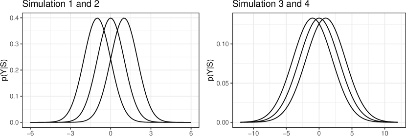
Figure 1: State-conditional response distributions in the simulation studies. In Simulation 1 and 2, states are reasonably well-separated, although there is still considerable overlap of the distributions. In Simulation 3 and 4, states less well-separated.

To assess the potential benefits of including a state-dependent missingness model in a HMM, we conducted a simulation study, focussing on a three-state hidden Markov model with a univariate Normal distributed response variable. We simulated four scenario’s. In Simulation 1 and 2 (Figure 1), the states are reasonably well-separated, with means $\mu_{1}=-1$, $\mu_{2}=0$, $\mu_{3}=1$ and standard deviations $\sigma_{1}=\sigma_{2}=\sigma_{3}=1$. Note that there is still considerable overlap in the state-conditional response distributions, as would be expected in many real applications of HMMs. In Simulation 1, missingness was state-dependent (i.e. MNAR), with $p(M_{t}=1|S_{t}=1)=.05$, $p(M_{t}=1|S_{t}=2)=.25$, and $p(M_{t}=1|S_{t}=2)=.5$. In Simulation 2, missingness was independent of the state (MAR), with $p(M_{t}=1|S_{t}=i)=p(M_{t}=1)=.25$. In Simulation 3 and 4 (Figure 1), the states were rather less well-separated, with means as for Simulation 1 and 2, but standard deviations $\sigma_{i}=3$. Here, the overlap of the state-conditional response distributions is much higher than in Simulation 1 and 2, and identification of the hidden states will be more difficult. In Simulation 3, missingness was state-dependent (MNAR) in the same manner as Simulation 1, while in Simulation 4, missingness was state-independent (MAR) as for Simulation 2. In all simulations, the initial state probabilities were $\pi_{1}=p(S_{1}=1)=.8$, $\pi_{2}=\pi_{3}=.1$, and the state-transition matrix was

$$\mathbf{A}=\left[\begin{matrix}.75&.125&.125\\ .125&.75&.125\\ .125&.125&.75\end{matrix}\right].$$

In each simulation, we simulated a total of 1000 data sets, each consisting of $N=100$ replications of a time-series of length $T=50$. We denote observations in such replicated time series as $Y_{i,t}$, with $i=1,\ldots,N$ and $t=1,\ldots,T$. Data was generated according to a 3-state hidden Markov model. For MAR cases, the non-missing observations are distributed as

$$p(Y_{i,t}|S_{i,t}=j)=\mathbf{Normal}(Y_{i,t}|\mu_{j},\sigma_{j}).$$ (13)

In the MNAR cases, the missingness variable $M$ and the response variable $Y$ were conditionally independent given the hidden state:

$$p(Y_{i,t},M_{i,t}|S_{i,t}=j)=\mathbf{Bernouilli}(M_{i,t}|\phi_{j})\times\mathbf{Normal}(Y_{i,t}|\mu_{j},\sigma_{j})$$ (14)

Data sets were simulated by first generating the hidden state sequences $S_{i,1:T}$ according to the initial state and transition probabilities. Then, the observations $Y_{i,1:T}$ were sampled according to the state-conditional distributions $p(Y_{i,t}|S_{i,t})$. Finally, random observations were set to missing values according to the missingness distributions $p(M_{i,t}|S_{i,t})$.

We fitted two 3-state hidden Markov models to each data-set. In the MAR models, observed responses were assumed to be distributed according to (13), and in the MNAR models, the observed responses and missingness indicators were assumed to be distributed according to (14). Parameters were estimated by maximum likelihood, using the Expectation-Maximisation algorithm, as implemented in depmixS4 (Visser & Speekenbrink, 2010). To speed up convergence, starting values were set to the true parameter values. Although such initialization is obviously not possible in real applications, we are interested in the quality of parameter estimates at the global maximum likelihood solution, and setting starting values to the true parameters makes it more likely to arrive at the global maximum. In real applications, one would need to use a sufficient number of randomly generated starting values to find the global maximum.

Table 1: Results of Simulation 1 (MNAR, low variance). Values shown are the true value of each parameter, and the mean (mean), standard deviation (SD), and mean absolute error (MAE) of the parameter estimates, for both the MAR and MNAR model. The value of ”rel. MAE” is the ratio of the mean absolute error of the MAR over the MNAR model.

		MAR			MNAR
parameter	true value	mean	SD	MAE	mean	SD	MAE	rel. MAE
$\mu_{1}$	-1.000	-1.010	0.131	0.094	-1.017	0.097	0.072	0.767
$\mu_{2}$	0.000	0.015	0.277	0.223	0.014	0.228	0.180	0.807
$\mu_{3}$	1.000	1.113	0.286	0.231	1.053	0.252	0.186	0.803
$\sigma_{1}$	1.000	0.998	0.051	0.033	0.995	0.034	0.026	0.785
$\sigma_{2}$	1.000	0.972	0.111	0.079	0.979	0.085	0.064	0.809
$\sigma_{3}$	1.000	0.959	0.104	0.077	0.979	0.085	0.061	0.801
$\pi_{1}$	0.800	0.834	0.146	0.117	0.776	0.110	0.083	0.715
$\pi_{2}$	0.100	0.118	0.152	0.111	0.131	0.130	0.105	0.944
$\pi_{3}$	0.100	0.049	0.048	0.062	0.093	0.066	0.055	0.890
$a_{11}$	0.750	0.774	0.080	0.064	0.743	0.055	0.039	0.613
$a_{12}$	0.125	0.144	0.094	0.068	0.139	0.077	0.061	0.896
$a_{13}$	0.125	0.082	0.055	0.057	0.118	0.054	0.044	0.765
$a_{21}$	0.125	0.144	0.086	0.065	0.124	0.062	0.048	0.729
$a_{22}$	0.750	0.759	0.116	0.087	0.754	0.096	0.070	0.812
$a_{23}$	0.125	0.097	0.082	0.068	0.122	0.075	0.058	0.850
$a_{31}$	0.125	0.146	0.085	0.068	0.118	0.050	0.039	0.579
$a_{32}$	0.125	0.166	0.128	0.103	0.138	0.092	0.070	0.679
$a_{33}$	0.750	0.688	0.111	0.090	0.744	0.076	0.056	0.623
$p(M=1|S=1)$	0.050	-	-	-	0.048	0.021	0.017	-
$p(M=1|S=2)$	0.250	-	-	-	0.247	0.073	0.057	-
$p(M=1|S=3)$	0.500	-	-	-	0.507	0.058	0.040	-

Table 2: Results of Simulation 2 (MAR, low variance). Values shown are the true value of each parameter, and the mean (mean), standard deviation (SD), and mean absolute error (MAE) of the parameter estimates, for both the MAR and MNAR model. The value of ”rel. MAE” is the ratio of the mean absolute error of the MAR over the MNAR model.

		MAR			MNAR
parameter	true value	mean	SD	MAE	mean	SD	MAE	rel. MAE
$\mu_{1}$	-1.000	-1.061	0.194	0.132	-1.062	0.200	0.134	1.014
$\mu_{2}$	0.000	-0.019	0.287	0.229	-0.022	0.288	0.230	1.005
$\mu_{3}$	1.000	1.048	0.213	0.158	1.038	0.213	0.157	0.991
$\sigma_{1}$	1.000	0.978	0.067	0.047	0.978	0.070	0.047	1.000
$\sigma_{2}$	1.000	0.969	0.105	0.079	0.969	0.107	0.081	1.021
$\sigma_{3}$	1.000	0.981	0.070	0.050	0.982	0.071	0.049	0.993
$\pi_{1}$	0.800	0.739	0.177	0.130	0.737	0.178	0.132	1.015
$\pi_{2}$	0.100	0.169	0.187	0.144	0.171	0.187	0.145	1.012
$\pi_{3}$	0.100	0.092	0.070	0.057	0.092	0.069	0.057	0.995
$a_{11}$	0.750	0.727	0.102	0.064	0.726	0.102	0.065	1.006
$a_{12}$	0.125	0.155	0.112	0.082	0.156	0.115	0.083	1.020
$a_{13}$	0.125	0.118	0.066	0.051	0.118	0.062	0.050	0.975
$a_{21}$	0.125	0.125	0.080	0.061	0.127	0.083	0.062	1.013
$a_{22}$	0.750	0.751	0.112	0.084	0.749	0.116	0.086	1.025
$a_{23}$	0.125	0.125	0.081	0.061	0.125	0.083	0.063	1.034
$a_{31}$	0.125	0.112	0.063	0.051	0.112	0.062	0.049	0.973
$a_{32}$	0.125	0.153	0.108	0.082	0.150	0.107	0.081	0.982
$a_{33}$	0.750	0.735	0.096	0.067	0.738	0.095	0.066	0.984
$p(M=1|S=1)$	0.250	-	-	-	0.250	0.046	0.027	-
$p(M=1|S=2)$	0.250	-	-	-	0.248	0.056	0.038	-
$p(M=1|S=3)$	0.250	-	-	-	0.247	0.046	0.028	-

Table 3: Results of Simulation 3 (MNAR, high variance). Values shown are the true value of each parameter, and the mean (mean), standard deviation (SD), and mean absolute error (MAE) of the parameter estimates, for both the MAR and MNAR model. The value of ”rel. MAE” is the ratio of the mean absolute error of the MAR over the MNAR model.

		MAR			MNAR
parameter	true value	mean	SD	MAE	mean	SD	MAE	rel. MAE
$\mu_{1}$	-1.000	-1.663	0.932	0.761	-1.198	0.628	0.315	0.414
$\mu_{2}$	0.000	-0.314	0.484	0.461	-0.110	0.470	0.409	0.888
$\mu_{3}$	1.000	1.480	1.214	0.923	1.383	0.956	0.609	0.661
$\sigma_{1}$	3.000	2.765	0.459	0.347	2.911	0.330	0.189	0.543
$\sigma_{2}$	3.000	2.889	0.455	0.302	2.967	0.333	0.215	0.713
$\sigma_{3}$	3.000	2.703	0.512	0.406	2.773	0.479	0.326	0.803
$\pi_{1}$	0.800	0.546	0.362	0.355	0.657	0.281	0.217	0.611
$\pi_{2}$	0.100	0.346	0.380	0.333	0.253	0.291	0.231	0.694
$\pi_{3}$	0.100	0.108	0.174	0.129	0.090	0.091	0.077	0.601
$a_{11}$	0.750	0.651	0.231	0.183	0.712	0.153	0.099	0.543
$a_{12}$	0.125	0.190	0.215	0.160	0.144	0.145	0.105	0.660
$a_{13}$	0.125	0.159	0.186	0.139	0.144	0.124	0.091	0.659
$a_{21}$	0.125	0.106	0.172	0.124	0.106	0.108	0.085	0.687
$a_{22}$	0.750	0.787	0.232	0.185	0.784	0.135	0.109	0.590
$a_{23}$	0.125	0.107	0.158	0.115	0.110	0.105	0.085	0.742
$a_{31}$	0.125	0.152	0.183	0.136	0.131	0.126	0.096	0.704
$a_{32}$	0.125	0.166	0.199	0.143	0.145	0.141	0.105	0.738
$a_{33}$	0.750	0.682	0.234	0.184	0.724	0.151	0.108	0.587
$p(M=1|S=1)$	0.050	-	-	-	0.076	0.122	0.059	-
$p(M=1|S=2)$	0.250	-	-	-	0.241	0.155	0.126	-
$p(M=1|S=3)$	0.500	-	-	-	0.489	0.134	0.092	-

Table 4: Results of Simulation 4 (MAR, high variance). Values shown are the true value of each parameter, and the mean (mean), standard deviation (SD), and mean absolute error (MAE) of the parameter estimates, for both the MAR and MNAR model. The value of ”rel. MAE” is the ratio of the mean absolute error of the MAR over the MNAR model.

		MAR			MNAR
parameter	true value	mean	SD	MAE	mean	SD	MAE	rel. MAE
$\mu_{1}$	-1.000	-1.650	1.002	0.801	-1.658	1.107	0.815	1.018
$\mu_{2}$	0.000	-0.171	0.539	0.432	-0.178	0.542	0.437	1.010
$\mu_{3}$	1.000	1.468	1.063	0.778	1.473	1.070	0.788	1.014
$\sigma_{1}$	3.000	2.719	0.468	0.383	2.720	0.473	0.375	0.981
$\sigma_{2}$	3.000	2.911	0.441	0.299	2.918	0.412	0.279	0.934
$\sigma_{3}$	3.000	2.728	0.504	0.377	2.732	0.478	0.365	0.968
$\pi_{1}$	0.800	0.528	0.345	0.352	0.522	0.338	0.357	1.012
$\pi_{2}$	0.100	0.330	0.367	0.316	0.344	0.359	0.320	1.014
$\pi_{3}$	0.100	0.141	0.199	0.149	0.134	0.192	0.142	0.951
$a_{11}$	0.750	0.638	0.230	0.183	0.645	0.220	0.177	0.968
$a_{12}$	0.125	0.188	0.212	0.155	0.182	0.211	0.155	0.998
$a_{13}$	0.125	0.174	0.188	0.139	0.174	0.178	0.134	0.963
$a_{21}$	0.125	0.111	0.166	0.121	0.103	0.157	0.119	0.984
$a_{22}$	0.750	0.774	0.223	0.175	0.787	0.209	0.170	0.972
$a_{23}$	0.125	0.114	0.152	0.111	0.110	0.139	0.110	0.986
$a_{31}$	0.125	0.133	0.169	0.125	0.137	0.167	0.124	0.997
$a_{32}$	0.125	0.167	0.193	0.138	0.162	0.186	0.139	1.007
$a_{33}$	0.750	0.700	0.232	0.177	0.701	0.224	0.176	0.992
$p(M=1|S=1)$	0.250	-	-	-	0.253	0.122	0.080	-
$p(M=1|S=2)$	0.250	-	-	-	0.237	0.086	0.056	-
$p(M=1|S=3)$	0.250	-	-	-	0.257	0.130	0.082	-

The results of simulation 1 (Table 1) show that, when states are relatively well separated, both models provide parameter estimates which are, on average, reasonably close to the true values. Both models have the tendency to estimate the means as more dispersed, and the standard deviations as slightly smaller, then they really are. While wrongly assuming MAR may not lead to overly biased estimates, we see that the mean absolute error (MAE) for the MNAR model is always smaller than that of the MAR model, reducing the estimation error to as much as 58%. As such, accounting for state-dependent missingness increases the accuracy of the parameter estimates. We next consider recovery of the hidden states, by comparing the true hidden state sequences to the maximum a posteriori state sequences determined by the Viterbi algorithm (see Rabiner, 1989; Visser & Speekenbrink, forthcoming). The MAR model recovers 53.13% of the states, while the MNAR model recovers 62.86% of the states. The accuracy in recovering the hidden states is thus higher in the model which correctly accounts for missingness. Whilst the performance of neither model may seem overly impressive, we should note that recovering the hidden states is a non-trivial task when the state-conditional response distributions have considerable overlap (see Figure 1) and states do not persist for long periods of time (here, the true self-transitions probabilities are $a_{ii}=.75$, meaning that states have an average run-length of 4 consecutive time-points). When ignoring time-dependencies and treating the observed data as coming from a bivariate mixture distribution over $Y$ and $M$, the maximum accuracy in classification would be 50.09% for this data. The theoretical maximum classification accuracy for the hidden Markov model is more difficult to establish, but simulations show that the MNAR model with the true parameters recovers 66.51% of the true states. For the MAR model, the approximate maximum classification accuracy is 58.06%.

The results of Simulation 2 (Table 2) show that when data is in fact MAR, both models provide roughly equally accurate parameter estimates. While the MNAR model does not provide better parameter estimates, including a model component for state-dependent missingness does not seem to bias parameter estimates compared to the MAR model. As can be seen, the state-wise missingness probabilities are, on average, close to the true values of .25. Over all parameters, the relative MAE of the models is 1.003 on average, which shows the models perform equally well. In terms of recovering the hidden states, the MAR model recovers 55.6% of the states, while the MNAR model recovers 55.63% of the states. The somewhat reduced recovery rate of the MNAR model compared to Simulation 1 is likely due to the fact that here, missingness provides no information about the identity of the hidden state. Here, the maximum classification accuracy is 42.91% for a mixture model, and approximately 60.45% for the hidden Markov models.

In Simulation 3 (Table 3) and 4 (Table 4) the states are less well-separated, making accurate parameter estimation more difficult. Here, the tendency to estimate the means as more dispersed and the standard deviations as smaller than they are becomes more pronounced. For both models the estimation error in Simulation 3 (Table 3) is larger than for Simulation 1, but comparing the MAE for both models again shows the substantial benefits for including a missingness model. Over all parameters, the relative MAE of the models is 0.658 on average, which shows the MNAR model clearly outperforms the MAR model. In terms of recovering the hidden states, the MAR model recovers 34.97% of the states, while the MNAR model recovers 45.27% of the states. As in Simulation 1, the MNAR model performs better in state identification. For both models, performance is lower than in Simulation 1, reflecting the increased difficulty due to increased overlap of the state-conditional response distributions (Figure 1). Indeed, the performance of the MAR model is close to chance (random assignment of states would give an expected accuracy of 33.33%). The maximum classification accuracy is 44.03% for a mixture model, and approximately 54.04% for the MNAR and 41.42% for the MAR hidden Markov models.

When missingness is ignorable (Simulation 4), Like in Simulation 2, inclusion of a missingness component in the HMM does not increase any bias in the parameter estimates. Over all parameters, the relative MAE of the models is 0.987 on average, which shows the models perform roughly equally well. The model which ignores missingness recovers 35.51% of the states, while the model with a missingness component recovers 35.5% of the states. For comparison, the maximum accuracy is 36.64% for a mixture model, and 42.51% for the hidden Markov models.

Taken together, these simulation results show that if missingness is state-dependent, there is a substantial benefit to including a (relatively simple) model for missingness in the HMM. When missingness is in fact ignorable, including a missingness model is superfluous, but does not bias the results. Hence, there appears to be little risk associated to including a missingness model into the HMM.

In a final simulation, we assessed the performance of the models when missingness is time-dependent, rather than state-dependent. Attrition is a common occurrence in longitudinal studies, meaning that the probability of missing data often increases with time. In this simulation, the probability of missing data varied with time $t$ through a logistic regression model:

$$p(M_{i,t}=1)=\frac{1}{1+\exp(-(0.125\times t-5))}.$$ (15)

Here, the probability of missing data is very small (0.008) at time 1, but increasing to rather high (0.777) at time 50. The other parameters were the same as in Simulation 1 and 2 (i.e., the states were relatively well-separated). In a model that specifies missingness as state-dependent, but not time-dependent, this could potentially result in biased parameter estimates. For instance, the increased probability of missingness over time may be accounted for by estimating states to have a different probability of missingness, and estimating prior and transition probabilities to allow states with a higher probability of missingness to occur more frequently later in time. In addition to the two hidden Markov models estimated before, we also estimated a hidden Markov model with a state- and time-dependent model for missingness:

$$p(M_{i,t}=1|S_{i,t}=j)=\frac{1}{1+\exp(-(\beta_{0,j}+\beta_{\text{time},j}\times t))}$$ (16)

This model should be able to capture the true pattern of missingness, whilst the MNAR model which only includes state-dependent missingness would not.

Table 5: Results of Simulation 5 (time-dependent missingness, low variance). Values shown are the true value of each parameter, and the mean (mean), standard deviation (SD), and mean absolute error (MAE) of the parameter estimates, for the MAR, MNAR (state), and MNAR (time) model. The value of ”rel. MAE 1” is the ratio of the mean absolute error of the MAR over the MNAR (state) model, and the value of ”rel. MAE 2” is the ratio of the mean absolute error of the MAR over the MNAR (time) model.

		MAR			MNAR (state)			MNAR (time)
parameter	true value	mean	SD	MAE	mean	SD	MAE	mean	SD	MAE	rel. MAE 1	rel. MAE 2
$\mu_{1}$	-1.000	-1.038	0.173	0.116	-0.825	0.076	0.176	-1.031	0.175	0.120	1.520	1.037
$\mu_{2}$	0.000	-0.015	0.272	0.215	-0.040	0.067	0.062	-0.020	0.294	0.233	0.287	1.086
$\mu_{3}$	1.000	1.033	0.195	0.143	0.757	0.084	0.243	1.029	0.207	0.153	1.698	1.068
$\sigma_{1}$	1.000	0.985	0.059	0.042	1.026	0.035	0.035	0.987	0.058	0.042	0.832	0.997
$\sigma_{2}$	1.000	0.967	0.111	0.082	1.278	0.033	0.278	0.966	0.112	0.083	3.370	1.010
$\sigma_{3}$	1.000	0.981	0.072	0.049	1.037	0.037	0.043	0.984	0.067	0.048	0.884	0.990
$\pi_{1}$	0.800	0.758	0.151	0.110	0.894	0.066	0.100	0.760	0.152	0.109	0.913	0.993
$\pi_{2}$	0.100	0.150	0.161	0.123	0.001	0.032	0.101	0.148	0.162	0.122	0.819	0.990
$\pi_{3}$	0.100	0.092	0.061	0.050	0.105	0.059	0.047	0.092	0.062	0.051	0.943	1.023
$a_{11}$	0.750	0.734	0.087	0.056	0.794	0.025	0.045	0.734	0.090	0.059	0.806	1.050
$a_{12}$	0.125	0.146	0.099	0.073	0.021	0.008	0.104	0.146	0.106	0.075	1.438	1.036
$a_{13}$	0.125	0.119	0.058	0.047	0.185	0.024	0.060	0.119	0.059	0.048	1.269	1.021
$a_{21}$	0.125	0.128	0.088	0.063	0.000	0.001	0.125	0.131	0.097	0.069	1.983	1.091
$a_{22}$	0.750	0.747	0.114	0.083	1.000	0.001	0.250	0.738	0.131	0.092	2.994	1.104
$a_{23}$	0.125	0.125	0.082	0.062	0.000	0.000	0.125	0.130	0.091	0.067	2.031	1.082
$a_{31}$	0.125	0.116	0.062	0.048	0.150	0.027	0.030	0.115	0.063	0.049	0.624	1.032
$a_{32}$	0.125	0.143	0.101	0.076	0.045	0.008	0.080	0.146	0.106	0.081	1.052	1.056
$a_{33}$	0.750	0.742	0.087	0.062	0.805	0.025	0.056	0.740	0.093	0.068	0.899	1.095
$\beta_{0,1}$	-5.000	-	-	-	-	-	-	-6.149	25.490	1.497	-	-
$\beta_{0,2}$	-5.000	-	-	-	-	-	-	-7.153	40.582	2.739	-	-
$\beta_{0,3}$	-5.000	-	-	-	-	-	-	-6.472	38.998	1.861	-	-
$\beta_{\text{time},1}$	0.125	-	-	-	-	-	-	0.154	0.605	0.039	-	-
$\beta_{\text{time},2}$	0.125	-	-	-	-	-	-	0.184	1.102	0.075	-	-
$\beta_{\text{time},3}$	0.125	-	-	-	-	-	-	0.188	1.815	0.074	-	-
$p(M=1|S=1)$	-	-	-	-	0.040	0.015	0.207	-	-	-	-	-
$p(M=1|S=2)$	-	-	-	-	0.552	0.024	0.305	-	-	-	-	-
$p(M=1|S=3)$	-	-	-	-	0.067	0.022	0.181	-	-	-	-	-

The results (Table 5) show that, compared to the MAR model, the MNAR model which misspecifies missingness as state-dependent is inferior, resulting in more biased parameter estimates. Over all parameters, the relative MAE of these two models is 1.353 on average, indicating the MAR model outperforms the MNAR (state) model. To account for the increase in missing values later in time, the MNAR (state) model estimates the probability of missingness as highest for state 2, which is estimated to have a mean of close to 0, but an increased standard deviation to incorporate observations from the other two states. To make state 2 more prevalent over time, transition probabilities to state 2 are relatively low from state 1 and 2 (parameters $a_{12}$ and $a_{32}$ respectively), whilst self-transitions ($a_{22}$) are close to 1 (meaning that once in state 2, the hidden state sequence is very likely to remain in that state. The prevalence of state 2 is thus increasing over time, and as this state has a higher probability of missingness, so is the prevalence of missing values. The MNAR (time) model, which allows missingness to depend on both the hidden states and time, performs only slightly worse than the MAR model, with an average relative MAE over all parameters of this model compared to the MAR of 1.042. However, the MNAR (time) model is able to capture the pattern of attrition (increased missing data over time), whilst the MAR model is not. As such, the MNAR (time) model may be deemed preferable to the MAR model, insofar as one is interested in more than modelling the responses $Y$. In terms of recovering the hidden states, the MAR model recovers 55.67% of the states, and the MNAR (time) model recovers 55.42% of the states. The misspecified MNAR (state) model recovers 50% of the states. The maximum classification accuracy for this data is 42.95% for a mixture model, and approximately 59.91% for the hidden Markov models.

This final simulation shows that when modelling patterns of missing data in hidden Markov models, care should be taken in how this is done. An increase in missing data over time could be due to an underlying higher prevalence of states which result in more missing data, and/or a state-independent increase in missingness over time. In applications where the true reason and pattern of missingness is unknown, it is then advisable to start by allowing for both state- and time-dependent missing data, selecting simpler options when this is warranted by the data.

3 Application: Severity of schizophrenia in a clinical trial

Here, we apply our hidden Markov model with state-dependent missingness to data from the National Institute of Mental Health Schizophrenia Collaborative Study. The study concerns the assessment of treatment-related changes in overall severity of mental illness. In this study, 437 patients diagnosed with schizophrenia were randomly assigned to receive either placebo (108 patients) or a drug (329 patients) treatment, and their severity of their illness was rated by a clinician at baseline (week 0), and at subsequent 1 week intervals (weeks 1–6), with week 1, 3, and 6 as the intended main follow-up measurements. This data has been made publicly available by Don Hedeker and has been analysed numerous times. In particular, Hedeker & Gibbons (1997) focused on pattern mixture methods to deal with missing data. Yeh et al. (2010) and Yeh et al. (2012) applied Markov and hidden Markov models, respectively, assuming ratings were MAR.

The analysis focuses on a single item of the Inpatient Multidimensional Psychiatric Scale (Lorr & Klett, 1966), which rates illness severity on a scale from 1 (“normal”) to 7 (“among the most extremely ill”).. Most participants were measured on week 0 (99.31%) and 1 (97.48%), whilst the other main measurement points at week 3 (85.58%) and 6 (76.66%) show more missing values. For a few participants, ratings were instead obtained on week 2 (3.2%), 4 (2.52%), and/or 5 (2.06%). Even when ignoring these rare deviations from the main measurement points, there is a clear potential issue with missing data and attrition, with 75.29% being measured the intended four times or more, and 15.1% rated on just three occasions, and 9.61% only twice. The distribution of the ratings at each week is shown in Figure 2. As can be seen there, ratings were generally relatively high at week 0, 1, and 3, but are relatively lower at week 6. As there are only a small number of ratings at week 2, 4, and 5, the empirical distributions for those weeks are rather unreliable.

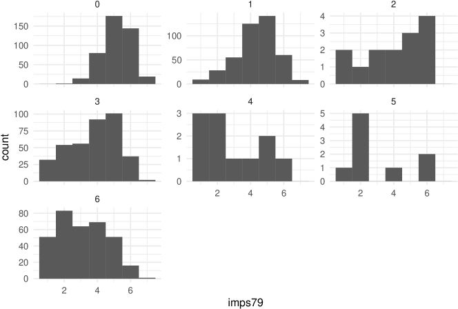
Figure 2: Distribution of the severity of illness ratings (IMPS item 79) at each week.

Table 6: Results of a logistic regression analysis modelling missingness as a function of drug, week, and whether the week was a main measurement occasion or not.

	$\hat{\beta}$	$\text{SE}(\hat{\beta})$	$z$	$P(>|z|)$
(Intercept)	1.921	0.393	4.884	0.000
drug	0.433	0.463	0.936	0.349
week	0.496	0.068	7.353	0.000
main	-5.381	0.382	-14.103	0.000
$\texttt{drug}\times\texttt{week}$	-0.112	0.081	-1.395	0.163
$\texttt{drug}\times\texttt{main}$	-0.596	0.446	-1.335	0.182

To gain initial insight into patterns underlying the missing data, we modelled whether the IMPS rating was missing or not with a logistic regression model. Predictors in the model were a dummy-coded variable drug (placebo = 0, medicine = 1), week (from 0 to 6) as a metric predictor, and a dummy-coded variable main to indicate whether the rating was at a main measurement week (i.e. at week 0, 1, 3, or 6). We also included an interaction between drug and week, and between drug and main. The results of this analysis (Table 6) show a positive effect of week (such that missingness increases over time), and a negative effect of main, with (many) more missing values on weeks which are not the main measurement weeks. The positive effect of week is a clear sign of attrition. A question now is whether this attrition is related to the severity of the illness, in which case the ratings at week 6 would provide a biased view on the true severity of illness after 6 weeks of treatment with a placebo or medicine. There are of course different methods to assess this, and many have been already applied to this particular dataset. Our objective here is to incorporate a model of missingness into a hidden Markov model, allowing missingness to depend on the latent state as well as observable features such as the measurement week.

3.1 Hidden Markov models

We fitted HMMs in which we either assumed ratings are MAR, or assume ratings are MNAR and state- and time-dependent. For each type of model (MAR or MNAR), we fit versions with 2, 3, 4, or 5 states. Both types of model assume imps79, the IMPS Item 79 ratings, follow a Normal distribution, with a state-dependent mean and standard deviation. No additional covariates were included, as the states are intended to capture all the important determinants of illness severity. To model effects of drug, we allow transitions between states, as well as the initial state, to depend on drug. Whilst the initial measurement at week 0 was made before administering the drug, we include a possible dependence to account for any potential pre-existing differences between the conditions. In the MNAR models, a second (dichotomous) response variable missing is included, in addition to imps79. The missing variable is modelled with a logistic regression, using week and the dummy-coded main variable as predictors, as these were found to be important predictors in the (state-independent) logistic regression analysis reported earlier. All models were estimated by maximum likelihood using the EM algorithm implemented in depmixS4 (Visser & Speekenbrink, 2010).

Table 7: Modelling results for the MAR and MNAR hidden Markov models with 2-5 latent states.

model	#states	log Likelihood	#par	AIC	BIC
MAR	2	-2422.675	16	4865.350	4919.146
	3	-2266.603	30	4577.206	4695.558
	4	-2225.871	48	4527.742	4732.168
	5	-2182.390	70	4480.781	4792.799
MNAR	2	-3074.628	22	6181.256	6267.330
	3	-2889.040	39	5840.081	6006.849
	4	-2841.108	60	5782.215	6051.197
	5	-2800.336	85	5746.671	6139.385

For both the MAR and MNAR models, the BIC indicates a three-state model fits best, whilst the AIC indicates a five-state model (or higher) fits best. Favouring simplicity, we follow the BIC scores here, and focus on the three-state models.

We first consider the estimates of the MAR model. The estimated means and standard deviations are

$$\mbox{\boldmath$\mu$}=[2.315,4.339,5.7]\quad\quad\mbox{\boldmath$\sigma$}=[0.821,0.619,0.567].$$

Hence, the states are ordered, with state 1 being the least severe, and state 3 the most severe. The prior probabilities of the states, for treatment with placebo and drug respectively, are

$$\mbox{\boldmath$\pi$}_{\text{placebo}}=[0,0.333,0.667]\quad\quad\mbox{\boldmath$\pi$}_{\text{drug}}=[0.005,0.307,0.689],$$

and the transition probability matrices (with initial states in rows and subsequent states in columns) are

$$\mathbf{T}_{\text{placebo}}=\left[\begin{matrix}0.963&0.004&0.032\\ 0.118&0.878&0.004\\ 0.027&0.046&0.927\end{matrix}\right]\quad\quad\mathbf{T}_{\text{drug}}=\left[\begin{matrix}1&0&0\\ 0.231&0.764&0.005\\ 0.073&0.307&0.62\end{matrix}\right].$$

As expected, the initial state probabilities show little difference between the treatments (as the initial measurement was conducted before treatment commenced), but the transition probabilities indicate that for those who were administered a real drug, transitions to less severe states are generally more likely, indicating effectiveness of the drugs. This is particularly marked for the most severe state, where the probability of remaining in that state is 0.927 with a placebo, but 0.62 with a drug.

We next consider the three-state MNAR model. The means and standard deviations are

$$\mbox{\boldmath$\mu$}=[2.325,4.424,5.756]\quad\quad\mbox{\boldmath$\sigma$}=[0.833,0.668,0.547]$$

showing the same ordering of states in terms of severity. The prior probabilities for placebo and drug groups are

$$\mbox{\boldmath$\pi$}_{\text{placebo}}=[0,0.393,0.607]\quad\quad\mbox{\boldmath$\pi$}_{\text{drug}}=[0.004,0.349,0.647],$$

and the transition probability matrices are

$$\mathbf{T}_{\text{placebo}}=\left[\begin{matrix}0.93&0.005&0.065\\ 0.123&0.872&0.005\\ 0.026&0.031&0.942\end{matrix}\right]\quad\quad\mathbf{T}_{\text{drug}}=\left[\begin{matrix}1&0&0\\ 0.239&0.761&0.001\\ 0.073&0.331&0.596\end{matrix}\right].$$

These estimates are close to those of the MAR model, indicating little initial difference between the conditions, but effectiveness of the drugs in the transition probabilities, which are higher towards the less severe states than for the placebo condition.

Table 8: Parameter estimates of the state dependent logistic regression models for missingness, with lower and upper reflecting the lower and upper bounds of the approximate $95\%$ confidence intervals.

state	parameter	estimate	lower	upper
1	(Intercept)	2.635	1.998	3.272
	week	0.149	0.028	0.269
	main	-4.511	-5.037	-3.984
2	(Intercept)	7.976	1.261	14.691
	week	-0.510	-1.978	0.959
	main	-13.014	-20.014	-6.014
3	(Intercept)	1.108	0.303	1.913
	week	0.710	0.538	0.883
	main	-5.029	-5.822	-4.235

Results of the state-dependent models for missingness are provided in Table 8. For all three states, the confidence interval for the effect of main excludes 0, indicating a significantly lower proportion of missing ratings at the main measurement weeks. In state 1 and 3, the confidence interval for the effect of week also excludes 0, indicating a higher rate of missing ratings over time, possibly due to attrition. For state 2, the effect of week is not significant. Figure 3 depicts the predicted probability of missing ratings for each state and week. This shows that in state 2, the chance of missing data on the main measurement weeks is small at $p(M_{t}|S_{t}=2)=0.003$, while it is high at $p(M_{t}|S_{t}=2)=0.997$ on the other weeks. In the other states, the probabilities are less extreme, with missing (and non-missing) data occurring on the main measurement weeks and the other weeks as well. In the final week 6, those in the most severe state 3 are the most likely to have missing data with $p(M_{t}|S_{t}=3)=0.585$. For those in the least severe state 1, the probability of missingness in week 6 is also substantial at $p(M_{t}|S_{t}=1)=0.272$.

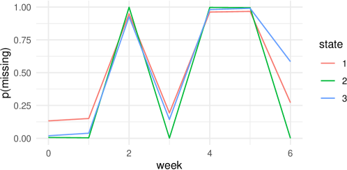
Figure 3: Predicted probability of missing IMPS Item 79 ratings by week for each state in the three-state MNAR hidden Markov model.

Disregarding the modelling of missingness, the parameters of the MAR and MNAR model seem reasonably close. This could be an indication that missingness is independent of the hidden states and data are possibly MAR. The likelihood of the MAR is not directly comparable to that of the MNAR model, as the latter is defined over two variables (the rating and the binary missing variable), while the former involves just a single variable. However, we can test for equivalence by fitting a constrained version of the MNAR model, where the parameters of the missingness model are constrained to be identical over the states. Unlike the MAR model, this restricted version of the MNAR model accounts for patterns of missingness, allowing these to depend on week and main, but not on the hidden state. A likelihood ratio test indicates that this restricted model fits less well, $\chi^{2}(6)=1328.57$ $p<.001$. Hence, there is evidence that the MNAR model is preferable to the MAR model and that missingness is indeed state-dependent.

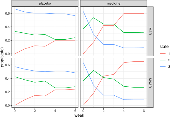
Figure 4: Proportions of maximum a posteriori (MAP) state assignments over weeks for the medication and placebo groups, according to the MAR and MNAR model.

Whilst the MAR and MNAR model provide roughly equivalent parameters for the severity ratings in the three states, when comparing the maximum a posteriori (MAP) state classifications from the Viterbi algorithm (Figure 4), we see that state classifications for the the MAR model tend to be for the more severe states. According to the MNAR model, during the main measuring weeks, missing values are relatively likely in the least severe state 1. Hence, those with missing values are more likely to be assigned to the least severe state. This is in line with the analysis of Hedeker & Gibbons (1997), who found evidence that dropouts in the medication condition showed more improvement in their symptoms.

It is worthwhile to note that the MAP states are also determined for time points with missing data, as the transition probabilities make certain states more probable than others, even when there is no direct measurement available. This provides a potentially meaningful basis to impute missing values, with another option being expected rating as a function of the posterior probability of all states. As imputation is not the focus of this study, we leave this to be investigated in future work.

4 Discussion

Previous work on missing data in hidden Markov models has mostly focussed on cases where missing values are assumed to be missing at random (MAR). Here, we addressed situations where data is missing not at random (MNAR), and missingness depends on the hidden states. Simulations showed that including a submodel for state-dependent missingness in a HMM is beneficial when missingness is indeed state-dependent, whilst relatively harmless when data is MAR. However, when the form of state-dependent missingness is misspecified (e.g. the effect of measurable covariates on missingness ignored), results may be biased. In practice, it is therefore advisable to consider the potential effect of covariates in the state-dependent missingness models. A reasonable strategy is to first model patterns of missingness through e.g. logistic regression, and then include important predictors from this analysis into the state-dependent missingness models. Applying this strategy to a real example about severity of schizophrenia in a clinical trial with substantial missing data, we showed that assuming data is MAR may lead to possible misclassification of patients to states (towards more severe states in this example). Whilst the ground truth is unavailable in such real applications, model comparison can be used to justify a state-dependent missingness model. Using flexible analysis tools such as the depmixS4 package (Visser & Speekenbrink, 2010) makes specifying, estimating, and comparing hidden Markov models with missing data specifications straightforward. There is then little reason to ignore potentially non-ignorable patterns of missing data in hidden Markov modelling.

Another approach to dealing with non-ignorable missingness (MNAR) is the pattern-mixture approach of Little 1993; 1994. The main idea of this approach is to group units of observations (e.g. patients) by the pattern of missing data, and allowing the parameters of a statistical model for the observations $Y$ to dependent on the missingness pattern $M_{1:T}$. There are certain similarities between this approach and modelling missingness as state-dependent. Rather than conditionalizing on a pattern of missing values, a hidden Markov model conditionalizes on a pattern (sequence) of hidden states, $s_{1:T}$, and the marginal distribution of the observations is effectively a multivariate mixture

$$p(Y_{1:T}|\mbox{\boldmath$\theta$})=\sum_{s_{1:T}\in\mathcal{S}^{T}}\sum_{m_{1:T}\in\mathcal{M}^{T}}p(Y_{1:T}|m_{1:T},s_{1:T},\mbox{\boldmath$\theta$})p(m_{1:T}|s_{1:T},\mbox{\boldmath$\theta$})p(s_{1:T}|\mbox{\boldmath$\theta$})$$ (17)

(note that $\theta$ here includes all parameters, so $\phi$). A pattern-mixture model would instead propose

$$p(Y_{1:T}|\mbox{\boldmath$\theta$})=\sum_{m_{1:T}\in\mathcal{M}^{T}}p(Y_{1:T}|m_{1:T},\mbox{\boldmath$\theta$})p(m_{1:T}|\mbox{\boldmath$\theta$}).$$ (18)

Trivially, if we set the number of hidden states to $K=1$, both models are the same. Another trivial equivalence is through a one-to-one mapping between $m_{1:T}$ and $s_{1:T}$. This could be obtained of by setting $K=2$, assuming the Markov process is of order $T$, and fixing e.g. $p(M_{t}=0|S=1)=1$ and $p(M_{t}=1|S=2)=1$. More interesting is to investigate cases where the procedures are similar, but not necessarily equivalent. The general pattern-mixture model is often underidentified (Little, 1993). For time-series of length $T$, there are $2^{T}$ possible missing data patterns. Without further restrictions, estimating the mean vectors and covariance matrices for all these components is not possible, due to the structural missing data in those patterns. The state-dependent MNAR hidden Markov model is identifiable insofar as the HMM for the observed variable $Y$ is identifiable. It is convenient, but not necessary, to assume a first-order Markov process. Higher-order Markov processes may allow the model to capture complex effects of missingness. Another option is to use the missingness indicator $M_{t}$ as a covariate on initial and transition probabilities, rather than a dependent variable. We leave investigation of such alternative models to future work.

References

- (1)
- Albert (2000) Albert, P. S. (2000), ‘A transitional model for longitudinal binary data subject to nonignorable missing data’, Biometrics 56(2), 602–608.
- Bahl et al. (1983) Bahl, L. R., Jelinek, F. & Mercer, R. L. (1983), ‘A maximum likelihood approach to continuous speech recognition’, IEEE Transactions on Pattern Analysis and Machine Intelligence PAMI-5(2), 179–190.
- Deltour et al. (1999) Deltour, I., Richardson, S. & Hesran, J.-Y. L. (1999), ‘Stochastic algorithms for markov models estimation with intermittent missing data’, Biometrics 55(2), 565–573.
- Hedeker & Gibbons (1997) Hedeker, D. & Gibbons, R. D. (1997), ‘Application of random-effects pattern-mixture models for missing data in longitudinal studies.’, Psychological Methods 2(1), 64.
- Little (1993) Little, R. J. (1993), ‘Pattern-mixture models for multivariate incomplete data’, Journal of the American Statistical Association 88(421), 125–134.
- Little (1994) Little, R. J. A. (1994), ‘A class of pattern-mixture models for normal incomplete data’, Biometrika 81(3), 471–483.
- Little & Rubin (2014) Little, R. J. & Rubin, D. B. (2014), Statistical analysis with missing data, 2 edn, John Wiley & Sons, Hoboken, NJ.
- Lorr & Klett (1966) Lorr, M. & Klett, C. J. (1966), Inpatient multidimensional psychiatric scale: Manual, Consulting Psychologists Press, Palo Alto, CA.
- Paroli & Spezia (2002) Paroli, R. & Spezia, L. (2002), ‘Parameter estimation of gaussian hidden markov models when missing observations occur’, Metron-International Journal of Statistics 60(3-4), 163–179.
- Rabiner (1989) Rabiner, L. R. (1989), ‘A tutorial on hidden Markov models and selected applications in speech recognition’, Proceedings of IEEE 77(2), 267–295.
- Rubin (1976) Rubin, D. B. (1976), ‘Inference and missing data’, Biometrika 63(3), 581–592.
-
Visser & Speekenbrink (2010)
Visser, I. & Speekenbrink, M. (2010), ‘depmixS4: An R package for hidden Markov
models’, Journal of Statistical Software 36(7), 1–21.
http://www.jstatsoft.org/v36/i07/ - Visser & Speekenbrink (forthcoming) Visser, I. & Speekenbrink, M. (forthcoming), Mixture and hidden Markov models with R, Springer.
- Yeh et al. (2012) Yeh, H.-W., Chan, W. & Symanski, E. (2012), ‘Intermittent missing observations in discrete-time hidden markov models’, Communications in Statistics-Simulation and Computation 41(2), 167–181.
- Yeh et al. (2010) Yeh, H.-W., Chan, W., Symanski, E. & Davis, B. R. (2010), ‘Estimating transition probabilities for ignorable intermittent missing data in a discrete-time markov chain’, Communications in Statistics—Simulation and Computation 39(2), 433–448.
- Yu & Kobayashi (2003) Yu, S.-Z. & Kobayashi, H. (2003), ‘A hidden semi-markov model with missing data and multiple observation sequences for mobility tracking’, Signal Processing 83(2), 235–250.
- Zucchini et al. (2017) Zucchini, W., MacDonald, I. L. & Langrock, R. (2017), Hidden Markov models for time series: an introduction using R, CRC press.