Backward asymptotics in S-unimodal maps.

Abstract

While the forward trajectory of a point in a discrete dynamical system is always unique, in general a point can have infinitely many backward trajectories. The union of the limit points of all backward trajectories through $x$ was called by M. Hero the “special $\alpha$-limit” ($s\alpha$-limit for short) of $x$. In this article we show that there is a hierarchy of $s\alpha$-limits of points under iterations of a S-unimodal map: the size of the $s\alpha$-limit of a point increases monotonically as the point gets closer and closer to the attractor. The $s\alpha$-limit of any point of the attractor is the whole non-wandering set. This hierarchy reflects the structure of the graph of a S-unimodal map recently introduced jointly by Jim Yorke and the present author.

To Jim Yorke, on the occasion of his 80th brithday.

1 Introduction

Our interest in $s\alpha$-limits comes from their relation to the edges of the graph of a dynamical system, that we studied in a recent joint work with J. Yorke [11] in case of S-unimodal maps. What we ultimately show in [11] is that, in the 1-dimensional real case, there is a hierarchy among repellors so that points arbitrarily close to a given repellor have trajectories that asymptote to all repellors below him in this hierarchy and to no other repellor. In [12] we present numerical evidence that this phenomenon is common also in multidimensional real discrete dynamical systems.

Due to this hierarchy, backward limits are much more complicated than in the 1-dimensional complex case, where there is, instead, a unique repellor, the Julia set, and this repellor is both backward and forward invariant. We believe that this is the main reason why the standard definition of $\alpha$-limit was never questioned by the discrete complex dynamics community. In this article, we argue that the concept of $s\alpha$-limit is a more suitable analogue of $\omega$-limit and use our results in [11] to find the $s\alpha$-limit of points of the interval under a S-unimodal map.

The idea of encoding the qualitative behavior of a dynamical system in a graph goes back to S. Smale that, in [39], proved that the non-wandering set $\Omega_{f}$ of an Axiom-A diffeomorphism $f$ of a compact manifold decomposes in a unique way as the finite union of disjoint, closed, invariant indecomposable subsets $\Omega_{i}$, on each of which $f$ is topologically transitive. Hence one can associate to $f$ a directed graph, describing its qualitative dynamics, whose nodes are these $\Omega_{i}$ and such that there is an edge from $\Omega_{j}$ to $\Omega_{i}$ if the stable manifold of $\Omega_{i}$ intersects the unstable manifold of $\Omega_{j}$.

A decade later C. Conley, in [7], widely generalized this idea to continuous finite-dimensional dynamical systems replacing the non-wandering set with the chain-recurrent set. One of the main advantages of using the chain-recurrent set is that on this set there is a natural equivalence relation, that does not extend in general to the non-wandering set, whose equivalence classes turns out to be the exact analogue of the indecomposable subsets of Axiom-A diffeomorphisms. Conley’s construction was later generalized to discrete dynamics by D. Norton [32] and to several other settings by other authors (see [12] for a detailed bibliography on the subject).

The chain-recurrent set ${\mathcal{R}}_{f}$ of a dynamical system $f$ on $X$ is defined via $\varepsilon$-chains, namely finite sequences of points each of which is within $\varepsilon$ from the image of the previous one under $f$ (see the next section for more precise definitions about the concepts used in this introduction). A point $x\in X$ is upstream from a point $y\in X$ if there is an $\varepsilon$-chain that starts at $x$ and ends at $y$ for every $\varepsilon>0$. We also say that $y$ is downstream from $x$. A point is chain-recurrent if it is upstream (or, equivalently, downstream) from itself.

The relation

$$x\sim y\hbox{ if }x\hbox{ is both upstream and downstream from }y$$

is an equivalence relation. We call nodes its equivalence classes and we associate to $f$ the graph $\Gamma_{f}$ having the nodes of ${\mathcal{R}}_{f}$ as its nodes and so that there is an edge from node $A$ to node $B$ if there is a bi-infinite trajectory (bitrajectory)

$$t=(\dots,t_{-2},t_{-1},t_{0},t_{1},t_{2},\dots),$$

whose limit points for $n\to-\infty$ lie in $A$ and those for $n\to+\infty$ lie in $B$. The dynamical relevance of $\Gamma_{f}$ comes from Conley’s decomposition theorem: given a continuous map $f$ of a compact metric space $X$ into itself, a point $x\in X$ either belongs to a node of $\Gamma_{f}$, and so it has some kind or “recurrent” dynamics, or is “gradient-like”, namely it defines an edge between two distinct nodes of $\Gamma_{f}$ (see [32], Thm. 4.10).

In [11] we studied the structure of the graph of a S-unimodal map and proved that such graph is always a tower, namely that there is an edge between each pair of nodes. Since there cannot be loops in the graph of a dynamical system, this means that there is a linear hierarchy among all nodes: there is a first node $N_{0}$ that has edges towards each other node, a node $N_{1}$ that has edges towards each other node except $N_{0}$ and so on up to the attracting node $N_{p}$. Each node but one is repelling and every repelling node, which can be either a cycle (for short we call cycle a periodic orbit) or a Cantor set, has an edge towards the attracting node.

Figure 1 shows the nodes of the logistic map $\ell_{\mu}(x)=\mu x(1-x)$, $\mu\in[2.9,4]$, that are visible at the picture’s resolution. The attracting nodes are painted in shades of gray, representing the density of a generic orbit of the attractor. There are five kinds of attracting nodes: type $A_{1}$, a cycle; type $A_{2}$, a cycle of intervals; type $A_{3}$, an adding machine; type $A_{4}$, a 1-sided attracting cycle belonging to a repelling Cantor set (taking place at the beginning of each window); type $A_{5}$ (see Thm. G about this complicated case, taking place at the end of each window). The repelling nodes are painted either in green (if they are cycle nodes) or in red (if they are Cantor set nodes). The picture also shows the curves $c_{k}=\ell_{\mu}^{k}(c)$, $k=1,\dots,4$, where $c=1/2$ is the critical point of the logistic map. The points $c_{k}$ play a fundamental role in the forward and backward dynamics of S-unimodal maps.

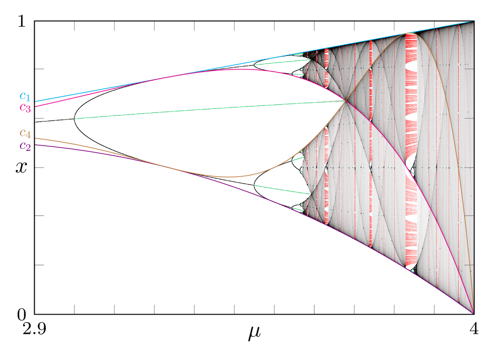
Figure 1: Bifurcations diagram of the logistic map. This picture shows the nodes of the logistic map $\ell_{\mu}(x)=\mu x(1-x)$ in the parameter range $[2.9,4]$ that are visible at this resolution. Attractors are painted in shades of gray (depending on the density), repelling periodic orbits in green and repelling Cantor sets in red. The colored lines labeled by $c_{k}$ are the lines $\ell_{\mu}^{k}(c)$, where $c=0.5$ is the critical point of $\ell_{\mu}$. The black dots that are visible within the diagram are points belonging to low-period cycles, signaling the presence of bifurcation cascades within some window. The fact that some of them keep close to the line $x=c$ is a reflection of Singer’s Theorem: when the attractor is a periodic orbit, $c$ belongs to its immediate basin. Notice that, for each $\mu$, all nodes but $N_{0}=0$ lie within the interval $[c_{2},c_{1}]$ since points in $(c_{1},1]$ are outside the range of the map and, for $\mu\geq 2$, all points in $(0,c_{2})$ eventually fall in $[c_{2},c_{1}]$, which is forward invariant. See Sec. 3.2 for further comments of this figure.

The main goal of the present article is to use our results in [11] to study the structure of the $s\alpha$-limit sets under S-unimodal maps. After presenting, in Sections 2 and 3, all definitions and main results we need from literature, we study in Section 4 the backward dynamics of points under a S-unimodal map $f:[0,1]\to[0,1]$, $f(0)=0$. Except when $N_{p}$ is of type $A_{5}$ (see Thm. 5 for a complete statement), our main result can be formulated as follows. When $f$ has $p$ nodes $N_{0},\dots,N_{p}$, $p\geq 1$, then $[0,1]$ can be written as the disjoint union of sets $U_{-1},U_{0},\dots,U_{p}$ such that:

1. each $U_{k}$, $k<p$, is the finite union of one or more intervals (these intervals can be open, half-open or closed);

2. $U_{-1}=(c_{2},1]$ is the set of all points that have no bitrajectory passing through them;

3. $U_{0}=[0,c_{2})$ is the set of all points with a single bitrajectory, which necessarily asymptotes backward to $0$;

4. $N_{k}\subset U_{k}$ for each $k=0,\dots,p$;

5. $U_{p}=N_{p}$;

6. $s\alpha_{f}(x)=\cup_{i=0}^{k}N_{i}$ for each $x\in U_{k}$, $k=0,\dots,p$;

Notice that proving this theorem requires different techniques for points that are not chain-recurrent and points that are so and, for chain-recurrent points, it requires different techniques for different types of nodes.

Figs. 6–8 show examples of these $U_{k}$ sets in several cases for the logistic map. For instance, let us describe $U_{1}$ in several cases when $\ell_{\mu}$ has three nodes. When $\mu$ is close enough to 3 from the right, $N_{1}=\{\bar{p}_{\mu}\}$ is the non-zero fixed point of $\ell_{\mu}$ and $N_{2}=\{p_{1},p_{2}\}$, $p_{1}<p_{2}$, a stable 2-cycle. In this case,

$$U_{1}=[c_{2},p_{1})\cup(p_{1},p_{2})\cup(p_{2},c_{1}].$$

When $\mu$ is a chaotic parameter with just three nodes and close enough from the left to $\mu_{M}\simeq 3.679$, which is the first parameter value at which $c_{3}$ and $c_{4}$ meet in Fig. 1, then $N_{1}=\{\bar{p}_{\mu}\}$ is again the non-zero fixed point of $\ell_{\mu}$ but this time $N_{2}=[c_{2},c_{4}]\cup[c_{3},c_{1}]$. Hence, in this case,

$$U_{1}=(c_{4},c_{3}).$$

When $\mu$ is close enough from the right to $\mu_{0}=1+2\sqrt{2}$, which is the left endpoint of the period-3 window (see Figs. 1 and 5), then $N_{1}$ is a Cantor set (painted in red) and $N_{2}=\{p_{1},p_{2},p_{3}\}$, $p_{3}<p_{1}<p_{2}$, is a stable 3-cycle (painted in black). Hence

$$U_{1}=[c_{2},p_{3})\cup(p_{3},p_{1})\cup(p_{1},p_{2})\cup(p_{2},c_{1}].$$

Our main result above achieves also two sub-goals. First, it proves for S-unimodal maps Conjecture 1 (see Sec. 2) by Kolyada, Misiurewicz and Snoha, namely that $s\alpha$ limits are closed sets for all $x\in[0,1]$. Second, it supports several numerical observations by the author in planar discrete dynamical systems [10] suggesting that, in case of real Newton maps on the plane, besides a non-trivial open set of points with backward trajectories that asymptote to (almost) the whole Julia set, just as it happens in the complex case (Theorem E), there are also non-trivial open sets from which one get smaller subsets of the non-wandering set or even the empty set.

2 Forward and Backward limits

The study of (time-)discrete dynamical systems, namely iterations of a continuous map $f:X\to X$ on a metric space $(X,d)$, goes back to the introduction of Poincaré maps [35, 36] as a tool to study the qualitative behavior of the integral trajectories of a vector field. One of the main goals of the field is finding the asymptotics of points under a given map $f$: where a point $x\in X$ ultimately ends up (the “$\omega$-limit” of $x$) and where it might come from (the “$\alpha$-limit” of $x$).

2.1 Forward asymptotics.

The asymptotics in the forward direction present no ambiguity: given a point $x\in X$, the set

$$\omega_{f}(x)=\bigcap_{n\geq 0}\;\overline{\bigcup_{m\geq n}\{f^{m}(x)\}}$$

consists in the accumulation points of the forward orbit of $x$, namely the sequence $\{f(x),f^{2}(x),f^{3}(x),\dots\}$ where, as usual, we use the notation

$$f^{n}(x)=f(f^{n-1}(x)).$$

The setting where discrete dynamics has been possibly more successful to date is iterations of holomorphic (and therefore rational) maps on the Riemann sphere ${\mathbb{CP}^{1}}$. In this setting, $F_{f}$ (Fatou set) denotes the largest open set over which the family of iterates $\{f^{n}\}$ is normal and $J_{f}$ (Julia set) its complement and we have the fundamental full classification below.

Definition 1.

We use cycle as a synonim for periodic orbit. By $n$-cycle we mean a periodic orbit of period $n$ (so, in particular, a $n$-cycle has $n$ elements). We denote by $|\gamma|$ the period of a cycle $\gamma$.

Theorem A ($\bm{\omega}$-limits in $\bm{{\mathbb{C}}}$ [40]).

Let $f:{\mathbb{CP}^{1}}\to{\mathbb{CP}^{1}}$ be a rational function of degree larger than 1. Then:

1. if $x\in J_{f}$, then $\omega_{f}(x)$ is either a repelling cycle or the whole $J_{f}$;

2. if $x\in F_{f}$, then $\omega_{f}(x)$ is either a hyperbolic or parabolic attracting cycle or a Jordan curve.

Recall that, in the complex setting, the duality non-chaotic versus chaotic dynamics coincides with the duality attracting versus repelling set. In the real case, except in particular cases such as Newton maps (e.g. see [9]), the two dualities are independent (for instance, there are chaotic attractors). In regard with orbits asymptotics, the latter is the most relevant. An analogue of Theorem A for the real case is given by the following weaker result:

Theorem B ($\bm{\omega}$-limits in $\bm{{\mathbb{R}}}$ [29]).

Let $f$ be either a generic non-invertible $C^{2}$ self-map of ${\mathbb{RP}^{1}}$ or a S-multimodal map on the interval. Then, for almost all $x$, $\omega_{f}(x)$ can be of the following three types:

1. a cycle;

2. a minimal Cantor set;

3. a finite union of closed intervals containing a critical point and on which $f$ acts transitively (see Def. 20).

The last case is the one where the dynamics within the attractor is chaotic, in the sense of sensitivity to initial conditions (see [22] and [37] for thorough discussions on alternate definitions of chaotic attractors).

2.2 Backward asymptotics.

The asymptotics in the backward direction have been explored much less, even in the two settings mentioned above. Traditionally, the $\alpha$-limit of a point is defined analogously to the $\omega$-limit:

$$\alpha_{f}(x)=\bigcap_{n\geq 0}\;\overline{\bigcup_{m\geq n}\{f^{-m}(x)\}}\,.$$

Notice that, in this case, in general $f^{-m}(x)$ consists in more than a single point and the growth of the number of counterimages with $m$ can be exponential. Very few theorems are known on $\alpha_{f}(x)$. We quote below the major ones known to us:

Theorem C ($\bm{\alpha}$-limits in $\bm{{\mathbb{C}}}$ [14]).

Let $f:{\mathbb{CP}^{1}}\to{\mathbb{CP}^{1}}$ be a rational function of degree larger than 1. Then, for all $z\in{\mathbb{CP}^{1}}$, with at most two exceptions, $\alpha_{f}(z)\supset J_{f}$. Moreover, $\alpha_{f}(z)=J_{f}$ if and only if $z$ belongs to either $J_{f}$ or to the basin of attraction of some stable cycle of $f$ (but not to the cycle itself).

As in case of $\omega$-limits, also the theorem above has a, much weaker, real analogue:

Theorem D ($\bm{\alpha}$-limits in $\bm{{\mathbb{R}}}$ [13]).

Let $f:{\mathbb{RP}^{1}}\to{\mathbb{RP}^{1}}$ be a generic analytic map and denote by $Z_{f}$ its set of critical points. Then $\alpha_{f}(Z_{f})=J_{f}$.

More recently, H. Cui and Y. Ding [8] studied in detail the $\alpha$-limit sets of S-unimodal maps.

2.3 $\alpha$-limits are not an optimal analogue of $\omega$-limits.

While the definition of $\alpha$-limit sets above has the appeal to be the precise analogue, replacing images with counterimages, of the definition of $\omega$-limit sets, the example below suggests that it does not represent necessarily the best answer to the question of “where might $x$ come from”.

Definition 2.

A bitrajectory of a map $f:X\to X$ based at $x\in X$ is a bi-infinite sequence $\{x_{i}\}_{i\in{\mathbb{Z}}}$ such that:

1. $x_{0}=x$;

2. $f(x_{i})=x_{i+1}$ for all $i\in{\mathbb{Z}}$.

Example 1.

Consider the logistic map $\ell_{\mu}(x)=\mu x(1-x)$ for some $\mu\in(1,4)$. The point $x=0$ is a repelling fixed point and $f(1)=0$, so $\alpha_{f}(0)=\{0,1\}$. For $x_{0}$ small enough, the equation $\ell_{\mu}(x)=x_{0}$ has 2 roots $x_{1},\hat{x}_{1}$ such that:

1. $x_{1}\in(0,x_{0})$;

2. $\hat{x}_{1}=1-x_{1}$ has no counterimage under $\ell_{\mu}$.

Hence $f^{-m}(x_{0})$ always consists in just two points $x_{m},\hat{x}_{m}$, with $x_{m}\to 0$ and $\hat{x}_{m}\to 1$. Ultimately, $\alpha_{f}(x_{0})=\{0,1\}$ for all $x_{0}$ small enough.

On the other side, every bitrajectory $\{t_{i}\}$ of $\ell_{\mu}$ passing through $x_{0}$ satisfies $\lim_{n\to-\infty}t_{n}=0$. Indeed, clearly the accumulation points of $\{t_{-i}\}_{i\in{\mathbb{N}}}$ belong to $\alpha_{f}(0)$ and, as long as $\mu<4$, $\ell_{\mu}(0.5)<1$ and so there is some neighborhood of 1 which is not in $\ell_{\mu}([0,1])$. In particular, no point close enough to 1 can belong to a bitrajectory of $\ell_{\mu}$.

In fact, an equivalent definition for $\alpha_{f}(x)$ is given by the following [21]:

Definition 3.

$\alpha_{f}(x)$ is the set of $y\in X$ for which there is a sequence of points $\{y_{n}\}$ and a sequence of monotonically increasing positive numbers $k_{n}$ such that:

1. $f^{k_{n}}(y_{n})=x$;

2. $\lim_{n\to\infty}y_{n}=y$.

Namely, arbitrarily close to each point in $\alpha_{f}(x)$, there are points whose forward trajectory passes through $x$.

The discussion above shows that, while formally there is a perfect symmetry between the definition of $\alpha$-limit and the one of $\omega$-limit, when a map is not invertible this symmetry does not extend to the sets obtained from those definitions: the $\omega$-limit set of a point $x$ contains only (and all) points that are asymptotically approached by $x$ under $f$, while its $\alpha$-limit contains also points that cannot be asymptotically approached, going backward, by a bitrajectory.

2.4 $s\alpha$-limits are a better analogue of $\omega$-limits.

A definition that leads to backward limit sets which are symmetric, from the point of view highlighted above, to $\omega$-limit sets can be achieved by slightly modifying the definition above:

Definition 4 ([21]).

Let $x\in X$. The special $\alpha$-limit $s\alpha_{f}(x)$ is the set of all $y\in X$ for which there is a sequence of points $\{y_{n}\}$ and a sequence of monotonically increasing positive numbers $k_{n}$ such that:

1. $y_{0}=x$;

2. $f^{k_{n}}(y_{n})=y_{n-1}$;

3. $\lim_{n\to\infty}y_{n}=y$.

The symmetry between $s\alpha_{f}$ and $\omega_{f}$ becomes evident when we write them in terms of limit points of trajectories $t$.

Definition 5.

Let $t$ be a bitrajectory. We denote by $\omega(t)$ (resp. $\alpha(t)$) the set of all forward (resp. backward) limit points of $t$.

Proposition 1.

Let $f:X\to X$ and $x\in X$. Then:

1. $\omega_{f}(x)=\omega(t)$ for any bitrajectory of $f$ based at $x$;

2. $s\alpha_{f}(x)=\cup\alpha(t)$, where the union is over all bitrajectories of $f$ based at $x$.

Not much is known on general properties of $s\alpha$-limit sets. The strongest claim related to them, in the author’s knowledge, is relative to infinite backward trajectories of rational maps on the Riemann sphere:

Theorem E ([20]).

Let $f$ be a rational map of degree larger than 1, $z_{0}$ a non-exceptional point and $\nu$ the equidistributed Bernoullli measure on the space of bitrajectories through $z_{0}$. Then, for $\nu$-almost all bitrajectories $t$ passing through $z_{0}$, we have that $\alpha(t)=J_{f}$.

Only recently several authors started a thorough investigation of its general properties, in particular F. Balibrea, J. Guirao and M. Lampart [2], J. Mitchell [31], J. Hantáková and S. Roth [18], S. Kolyada, M. Misiurewicz and L. Snoha [23]. In particular, the last three authors formulated the following conjecture:

Conjecture ([23]).

For all continuous maps of the interval, all $s\alpha$-limit sets of points are closed.

3 Definitions and graph of S-unimodal maps.

A discrete dynamical system on a metric space $(X,d)$ is given by the iterations of a continuous map $f:X\to X$. In this article we are interested in the case where $X$ is a closed interval and $f$ is a S-unimodal map, as defined below:

Definition 6 ([38]).

A $C^{3}$ map $f:[a,b]\to[a,b]$ is S-unimodal if:

1. either $f(a)=f(b)=a$ or $f(a)=f(b)=b$;

2. $f$ has a unique critical point $c\in(a,b)$;

3. the Schwarzian derivative of $f$

   $$Sf(x)=\frac{f^{\prime\prime\prime}(x)}{f^{\prime}(x)}-\frac{3}{2}\left(\frac{f^{\prime\prime}(x)}{f^{\prime}(x)}\right)^{2}$$

   is negative for all $x\in[a,b]$, $x\neq c$.

In all statements and examples throughout the article, we will assume that $c$ is a maximum. Of course the same proofs hold also when $c$ is a minimum after trivial modifications that we leave to the reader.

Given any S-unimodal map $f$, the equation $f(x)=y$ has two distinct solutions for each $y<f(c)$. For each $p\neq c$ in the domain of $f$, we denote by ${\hat{p}}$ the solution different from $p$ of the equation $f(x)=f(p)$.

Example 2.

In case of the logistic map

$$\ell_{\mu}(x)=\mu x(1-x)$$

we have that $[a,b]=[0,1]$, $f(0)=f(1)=0$, $c=0.5$ and $\hat{p}=1-p$. The Schwarzian derivative of $\ell_{\mu}$ is trivially negative since $\ell^{\prime\prime\prime}_{\mu}\equiv 0$.

Recall that, as a consequence of Guckenheimer’s results in [16], each S-unimodal map is topologically conjugated to a logistic map (see Thm. 6.4 and Remark 1 in [13]). In particular, each S-unimodal map has at most two fixed points.

The following several definitions are needed to define the graph of a dynamical system $f$.

Definition 7 ([4]).

An $\varepsilon$-chain from $x\in X$ to $y\in X$ is a sequence of points $x_{0}=x,x_{1},\dots,x_{n},x_{n+1}=y$ such that $d(f(x_{i}),x_{i+1})<\varepsilon$ for all $i=0,\dots,n$. We say that $x$ is downstream (resp. upstream from $y$) if, for every $\varepsilon>0$, there is an $\varepsilon$-chain from $y$ to $x$ (resp. from $x$ to $y$). A point $x\in X$ is chain-recurrent if it is downstream from itself.

3.1 Nodes.

We denote the set of all chain-recurrent points of $X$ under $f$ by ${\mathcal{R}}_{f}$. The relation $x\sim y$ iff $x$ is both upstream and downstream from $y$ is an equivalent relation in ${\mathcal{R}}_{f}$ (e.g. see [32]). The points of ${\mathcal{R}}_{f}/\sim$ will be the nodes of the graph and so we refer to them as nodes. Notice that every node is closed and invariant under $f$ [32]. The edges of the graph will be defined through the asymptotics of the system’s bitrajectories, as explained below.

Proposition 2 ([32]).

Given any bitrajectory $t$, there exist nodes $N_{1},N_{2}$ in ${\mathcal{R}}_{f}$, not necessarily distinct, such that $\alpha(t)\subset N_{1}$ and $\omega(t)\subset N_{2}$.

Proof.

If $x,y\in\omega(t)$ it means that, for every $\varepsilon>0$, there are integers $p,q,r$ such that $|x_{i}-x|<\varepsilon$ for $i=p,r$ and $|x_{q}-y|<\varepsilon$, namely $x$ is both upstream and downstream from $y$ and so they belong to the same node. The same argument can be repeated in case of the $\alpha$-limit. ∎

Notice that, when $\alpha(t)$ and $\omega(t)$ belong to the same node $N$, it means that all points of $t$ actually belong to $N$.

Definition 8 ([30]).

A closed invariant set $A$ is an attractor if it satisfies the following conditions:

1. the basin of attraction of $A$, namely the set of all $x\in X$ such that $\omega(x)\subset A$, has strictly positive measure;

2. there is no strictly smaller invariant closed subset $A^{\prime}\subset A$ whose basin differs from the basin of $A$ by just a zero-measure set.

Definition 9.

We call a node an attracting node if it contains an attractor, otherwise we call it a repelling node.

Definition 10.

We say that a cycle $\gamma$ is critical, regular or flip if, given any $p\in\gamma$, respectively $(f^{n})^{\prime}(p)=0$, $(f^{n})^{\prime}(p)>0$ or $(f^{n})^{\prime}(p)<0$.

Notice that the definition is consistent because the derivative of $f^{n}$ is constant on any $n$-cycle. Recall also that this derivative is zero, and so the cycle is superattracting, if and only if $c$ belongs to the cycle.

Definition 11.

We call period-$k$ trapping region of $f$ a collection ${\mathcal{T}}$ of $k$ closed intervals $J_{1},\dots,J_{k}$ such that:

1. $c$ lies in the interior of $J_{1}$;

2. the interiors of the $J_{i}$ are pairwise disjoint;

3. $f(J_{i})\subset J_{i+1}$, $i=1,\dots,k$, where we use the notation $J_{k+1}=J_{1}$.

We say that ${\mathcal{T}}$ is cyclic if, moreover,

1. $\partial J_{1}=\{p_{1},\hat{p}_{1}\}$ for some periodic point $p_{1}$;

2. $f(\partial J_{i})\subset\partial J_{i+1}$.

We denote by $|{\mathcal{T}}|$ the period of ${\mathcal{T}}$. When ${\mathcal{T}}$ is cyclic, we denote by $\Gamma({\mathcal{T}})$ the periodic orbit passing through $p_{1}$. We say that $\Gamma({\mathcal{T}})$ is the minimal cycle of ${\mathcal{T}}$ (see Thm. F). In general, we say that a cycle $\gamma$ is minimal when $\gamma=\Gamma({\mathcal{T}})$ for some trapping region ${\mathcal{T}}$. Sometimes, to emphasize, we denote by $J_{i}({\mathcal{T}})$ the $J_{i}$ interval of ${\mathcal{T}}$. We denote by $J^{int}=J^{int}({\mathcal{T}})$ the union of the interiors of all the $J_{i}$. We say that a cyclic trapping region is a flip trapping region if any two $J_{i}$ have an endpoint in common, otherwise we say it is a regular trapping region.

Proposition 3.

A cyclic trapping region ${\mathcal{T}}$ is flip (resp. regular) iff $\Gamma({\mathcal{T}})$ is flip (resp. regular). Moreover, $|{\mathcal{T}}|=|\Gamma({\mathcal{T}})|$ if ${\mathcal{T}}$ is regular while $|{\mathcal{T}}|=2|\Gamma({\mathcal{T}})|$ if ${\mathcal{T}}$ is flip.

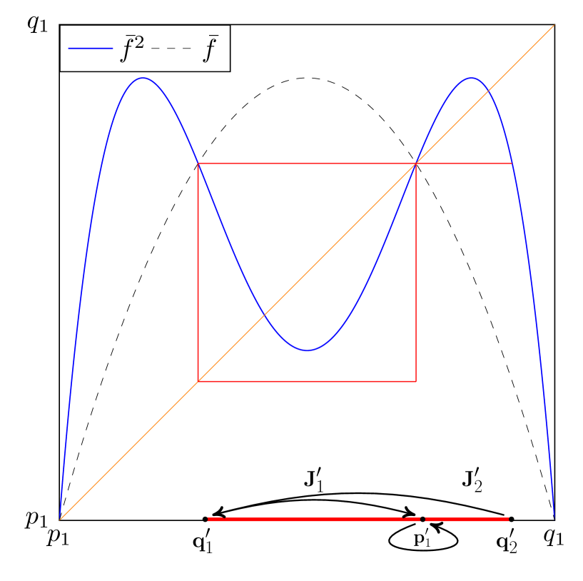
Figure 2: Example of flip trapping region. The interval $[p_{1},q_{1}]$, where possibly $q_{1}<p_{1}$, is the $J_{1}$ interval of some cyclic trapping region of some period $r$ of a map $f$, so that $J_{1}$ is invariant under $\bar{f}=f^{k}$. Inside $J_{1}$ is shown a period-2 flip trapping region $\{J^{\prime}_{1},J^{\prime}_{2}\}$ of $\bar{f}$. The point $p^{\prime}_{1}$, which is fixed by $\bar{f}$, is an endpoint of both $J^{\prime}_{1,2}$. Both the other endpoints $q^{\prime}_{1},q^{\prime}_{2}$ eventually fall on $p^{\prime}_{1}$. Notice that $\bar{f}(c)<q^{\prime}_{2}$.

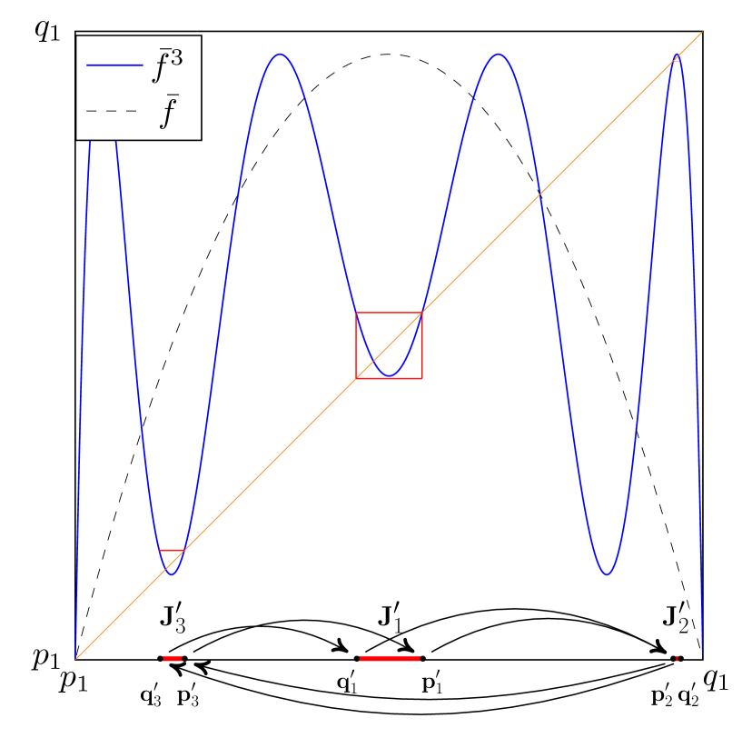
Figure 3: Example of regular trapping region. The interval $[p_{1},q_{1}]$, where possibly $q_{1}<p_{1}$, is the $J_{1}$ interval of some cyclic trapping region of some period $r$ of a map $f$, so that $J_{1}$ is invariant under $\bar{f}=f^{k}$. Inside $J_{1}$ is shown a period-3 regular trapping region $\{J^{\prime}_{1},J^{\prime}_{2},J^{\prime}_{3}\}$ of $\bar{f}$. The arrows show how the endpoints map under $\bar{f}$: the endpoints $p^{\prime}_{1},p^{\prime}_{2},p^{\prime}_{3}$ form an unstable 3-cycle of $\bar{f}$ and all other endpoints $q^{\prime}_{1},q^{\prime}_{2},q^{\prime}_{3}$ eventually fall into this cycle.

Example 3.

The interval $[a,b]$ is, trivially, a period-1 regular cyclic trapping region for every S-unimodal map.

Example 4.

Let $\bar{p}_{\mu}$ be the fixed point of the logistic map $\ell_{\mu}$ other than $0$. The collection

$${\mathcal{T}}_{\mu}=\{J_{1}=[\ell^{2}_{\mu}(c),\bar{p}_{\mu}],J_{2}=[\bar{p}_{\mu},\ell_{\mu}(c)]\}$$

is a period-2 trapping region for all $\mu\in(1+\sqrt{5},4]$. A direct calculation shows that ${\mathcal{T}}_{\mu}$ is cyclic only at

$$\mu_{M}=3[1+(19-3\sqrt{33})^{1/3}+(19+3\sqrt{33})^{1/3}]/2\simeq 3.67857,$$

which is exactly the point at which $\bar{p}_{\mu}$ plunges into a chaotic attractor and ceases to be a node in itself. At that point, the logistic map has a crisis [15].

This example above can be generalized to S-unimodal maps, as shown below.

Definition 12.

We call core of a S-unimodal map $f$ the interval $[f^{2}(c),f(c)]$.

In order to simplify the notation, we often use the notation $c_{k}$ in place of $f^{k}(c)$.

Proposition 4.

Let $f$ be a S-unimodal map and $\bar{p}$ its internal fixed point. The core of $f$ is forward-invariant if and only if $\bar{p}>c$.

Proof.

Notice first of all that, when $c_{3}<c_{2}<c$, we have that the restriction of $f$ to $[c_{3},c_{2}]$ is a orientation-preserving homeomorphism and so $f([c_{3},c_{2}])=[c_{4},c_{3}]$. Hence, in general, $f([c_{k},c_{k-1}])=[c_{k+1},c_{k}]$, namely the forward orbit of $c$ is a monotonically decreasing sequence contained in $[a,c)$ and therefore it must converge to a fixed point at the left of $c$. In particular, when $c<\bar{p}$, this cannot happen because, when $f$ has two fixed points, the boundary one $x=a$ is repelling (recall that $f$, being topologically conjugate to a logistic map, cannot have more than two fixed points). Now let us go over all possible cases:

Case 1: $\bm{\bar{p}\leq c}$. Since $f$ is monotonically increasing at the left of $c$ and monotonically decreasing at its right, this can happen if and only if the graph of $f$ is not above the diagonal at $x=c$, namely we must have $c_{1}\leq c$. The case $c_{1}=c$ is degenerate: in that case $c=\bar{p}$ is fixed and $[c_{2},c_{1}]$ is a single point. When $c_{1}<c$, the restriction of $f$ to $[c_{1},c]$ is a orientation-preserving homeomorphism and we fall again in the case outlined above: $f([c_{1},c])=[c_{2},c_{1}]$ and $f([c_{2},c_{1}])=[c_{3},c_{2}]$, so in particular $[c_{2},c_{1}]$ is not forward invariant.

Case 2: $\bm{c<\bar{p}}$, $\bm{c\leq c_{2}}$. In this case, the restriction of $f$ to $[c_{2},c_{1}]$ is a orientation-reversing homeomorphism and so $f([c_{2},c_{1}])=[c_{2},c_{3}]\subset[c_{2},c_{1}]$, showing that $c_{2}<c_{3}$ and that $[c_{2},c_{1}]$ is forward-invariant. It is not a trapping region, though, since $c\not\in(c_{2},c_{1})$.

Case 3: $\bm{c_{2}<c<\bar{p}}$. In this case, we have that

$$f([c_{2},c_{1}])=f([c_{2},c]\cup[c,c_{1}])=[c_{3},c_{1}]\cup[c_{2},c_{1}]=[c_{2},c_{1}]$$

since, by our argument above, the configuration $c_{3}<c_{2}<c<\bar{p}$ cannot take place and therefore we must have $c_{2}\leq c_{3}$. Hence in this case $[c_{2},c_{1}]$ is a period-1 trapping region. ∎

Several examples of cyclic flipping and regular trapping regions are shown, respectively, in Figs. 2,4 and 3,5.

Theorem F (Repelling Nodes [11]).

Let $f$ be a S-unimodal map. Then the minimum distance between a repelling node $N$ and the critical point of $f$ is achieved at a periodic point $p_{1}$ of $N$. The closed interval with endpoints $p_{1}$ and $\hat{p}_{1}$ is the $J_{1}$ interval of a cyclic trapping region ${\mathcal{T}}(N)$ such that:

1. $N\cap J^{int}({\mathcal{T}}(N))=\emptyset$;

2. $p_{1}\in\Gamma({\mathcal{T}}(N))$ and each interval of ${\mathcal{T}}(N)$ has a point of $\Gamma({\mathcal{T}}(N))$ at its boundary;

Depending on the type of the corresponding trapping region, there are two types of repelling nodes:

1. A flip cycle. In this case, ${\mathcal{T}}(N)$ is a flip trapping region.

2. A Cantor set with a dense orbit. In this case, ${\mathcal{T}}(N)$ is a regular trapping region.

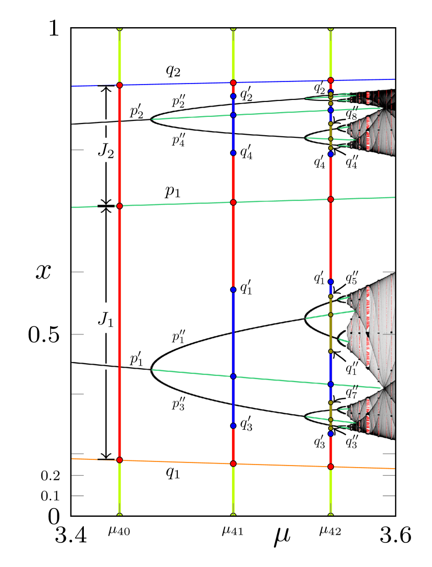
Figure 4: Examples of flipping trapping regions. This picture is discussed in detail in Sec. 3.4.

In order to keep notation light, we often write $\Gamma(N)$ to denote $\Gamma({\mathcal{T}}(N))$ and so on.

Remark 1.

A flip cycle node $N$ is always inside the interior of the union of all $J_{i}(N)$ (see Fig. 4). On the contrary, a Cantor set node $M$ has no point in common with the interior of the union of all $J_{i}(M)$ (see Fig. 5).

Theorem G (Attracting Nodes [11]).

Let $f$ be a S-unimodal map. Then its attracting nodes are of the following types:

1. An attracting cycle.

2. An attracting trapping region.

3. An attracting minimal Cantor set (this is the case when there are infinitely many nodes).

4. A repelling Cantor set containing a 1-sided attracting periodic orbit.

5. A trapping region which strictly contains an attracting cyclic trapping region, a repelling Cantor set and part of the basin of attraction. The Cantor set and the attractor have a 1-sided attracting periodic orbit in common.

Remark 2.

Among the attracting and repelling nodes of S-unimodal maps, those of type $A_{5}$ are the only ones containing points that are not non-wandering points. In particular, since all points in $\omega(t)$ and $\alpha(t)$ are non-wandering points, this is the only node that cannot be equal to either the $\omega$-limit or the $\alpha$-limit of any bitrajectory.

3.2 Examples of nodes.

Some of the nodes of the logistic map are shown in Fig. 1.

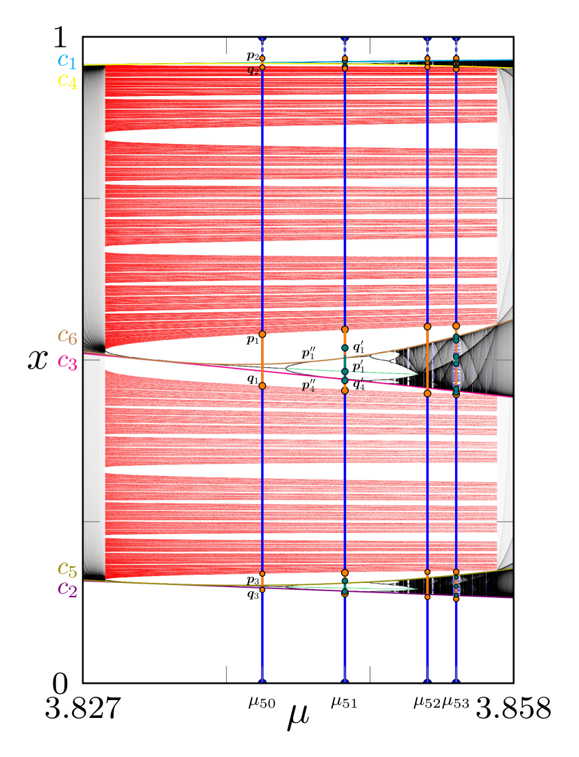
Figure 5: Examples of regular trapping regions. This picture is discussed in detail in Sec. 3.4.

Repelling nodes of type $R_{1}$ (resp. $R_{2}$) are painted in green (resp. red). Each repelling node of either kind exists over some closed connected interval of parameter values and depends continuously on it. The parameters range over which a repelling Cantor set node $N$ arise is called a window $W(N)$. The period of $W(N)$ is the period of the periodic point $p_{1}(N)$. The largest window of the logistic map family, shown in detail in Fig. 5, is the period-3 window starting at $\mu=1+2\sqrt{2}\simeq 3.828$ and ending at $\mu\simeq 3.857$ (see [19], p. 299, for an exact expression of this last number).

Attractors are shown in shades of gray. Attractors of type $A_{1}$ (isolated black lines) and of type $A_{2}$ are both visible. Attractors of type $A_{4}$ and $A_{5}$ are located, respectively, at the beginning and end of each window [11]. Attractors of type $A_{3}$ are not visible because they arise only for a zero-measure set of parameter values [27]. The lines visible throughout the chaotic attractors are iterates of the critical point, about which the density of points under iterations is higher. In colors are highlighted the first four of these iterates.

3.3 The Graph.

Finally we have all ingredients to introduce the graph of a discrete dynamical system:

Definition 13 ([7]).

We call graph $\Gamma_{f}$ of the dynamical system $f$ on $X$ the directed graph having as nodes the elements of ${\mathcal{R}}_{f}/\sim$ and having an edge from node $N_{1}$ to node $N_{2}$ when there exist a bitrajectory $t$ such that $\alpha(t)\subset N_{1}$ and $\omega(t)\subset N_{2}$.

The key result by Conley, obtained originally for continuous systems [7] and generalized later by D. Norton [33] to discrete ones, is that the dynamics outside of nodes is purely of gradient-like nature, as explained below.

Definition 14.

A Lyapunov function [42] for $f:X\to X$ is a continuous function $L$ such that:

1. $L$ is constant on each node;

2. $L$ assumes different values on different nodes;

3. $L(f(x))<L(x)$ if and only if $x$ is not chain-recurrent.

Theorem H ([33]).

Let $f$ be a dynamical system on a compact metric space $X$. Then there exists a Lyapunov function for $f$. In other words, every point $x\in X$ either belongs to ${\mathcal{R}}_{f}$ or is gradient-like for $f$.

Recall that a loop in a graph is a sequence of nodes $N_{1},N_{2},\dots,N_{k}$ such that there is an edge from $N_{i}$ to $N_{i+1}$ for $i=1,\dots,n-1$ and then an edge from $N_{k}$ back to $N_{1}$.

Corollary 1.

A graph $\Gamma_{f}$ does not have loops.

Definition 15.

A graph $\Gamma_{f}$ is a tower if there is an edge between each pair of nodes.

Notice that, because of the corollary above, if there is an edge from $A$ to $B$ then there cannot be an edge from $B$ to $A$.

In [11] we prove the following two fundamental results. Notice that the second theorem integrates some original result of ours together with other classic results by other authors (references are provided within the claim).

Theorem I (Tower Theorem.).

The graph of a S-unimodal map is a tower.

Theorem J (Chain-Recurrent Spectral Theorem).

Let $f$ be a S-unimodal map with at least a repellor and denote by $N_{0},N_{1},\dots,N_{p}$, where $p\geq 1$ is possibly infinite, the nodes of $\Gamma_{f}$ sorted in the order determined by the edges (in particular, $N_{p}$ is the attracting node of $f$). Then:

1. $N_{0}$ is the fixed endpoint of $f$.

2. Each repelling node $N_{i}$, $0\leq i<p$, determines a cyclic trapping region ${\mathcal{T}}(N_{i})$ for $f$ such that $\Gamma({\mathcal{T}}(N_{i}))\subset N_{i}$ and each $J_{k}({\mathcal{T}}(N_{i}))$ has a point of $\Gamma({\mathcal{T}}(N_{i}))$ as an endpoint. There is no other point of $N_{i}$ in ${\mathcal{T}}(N_{i})$ [11].

3. The trapping regions ${\mathcal{T}}(N_{i})$ are nested:

   $$\overline{J^{int}({\mathcal{T}}_{j})}\subset J^{int}({\mathcal{T}}_{j-1}),\;1\leq j<p,$$

   where, by convention, we take ${\mathcal{T}}(N_{0})=\{[a,b]\}$ [11].

4. Each $N_{j}$, $1\leq j<p$, is either of type $R_{1}$ or $R_{2}$ [11]. The measure of each repelling node is zero and the action of $f$ on it is topologically conjugated to a subshift of finite type [41].

5. Each $N_{j}$, $0\leq j<p$, is repelling and hyperbolic [41].

6. $N_{p}$ is the unique attracting node of $f$ [16] and it is one of the five types $A_{1},\dots,A_{5}$ [11].

7. $N_{p}$ is hyperbolic unless it is of type $A_{4}$ or $A_{5}$ [41].

8. In each neighborhood of $N_{i}$, for each $j\geq i$, there are points falling eventually into $N_{j}$ [11].

9. When $p=\infty$, the attracting node $N_{\infty}$ is a Cantor set of zero Lebesgue measure on which $f$ acts as an adding machine [41].

3.4 Examples of trapping regions.

Several cyclic trapping regions are shown in Figs. 4 and 5 in case of the logistic map. In all cases, the top node is $N_{0}=0$ and its corresponding trapping region is the interval $J_{1}(N_{0})=[0,1]$.

In Fig. 4 it is shown the logistic map’s bifurcation diagram for $\mu\in[3.4,3.6]$. Attracting cycles are shown in black. In this range, most of the figure is occupied by the first bifurcation cascade of the diagram. Throughout this range, the first node $N_{0}$ is the unstable fixed point 0 and the second node $N_{1}$ is the other fixed point $p_{1}$ (painted in green), which is unstable too. We show respectively in orange and blue the points $q_{1}=\hat{p}_{1}=1-p_{1}$ and $q_{2}$, where $q_{2}$ is the root of $\ell_{\mu}^{2}(x)=p_{1}$ on the other side of $q_{1}$ with respect to $p_{1}$ (see Fig. 3). We paint in lime ${\mathcal{T}}(N_{0})$.

At $\mu_{40}$, the logistic map has a third and final node: the attracting 2-cycle $N_{2}=\{p^{\prime}_{1},p^{\prime}_{2}\}$. The flip trapping region ${\mathcal{T}}(N_{1})$, painted in red, consists of the following two intervals: $J_{1}(N_{1})=[q_{1},p_{1}]$ and $J_{2}(N_{1})=[p_{1},q_{2}]$.

Between $\mu_{40}$ and $\mu_{41}$, the 2-cycle $N_{2}$ bifurcates and becomes repelling and a new attracting 4-cycle node $N_{3}=\{p^{\prime\prime}_{1},\dots,p^{\prime\prime}_{4}\}$ arises. We paint in blue the period-4 flip trapping region ${\mathcal{T}}(N_{2})$, which consists in the following intervals: $J_{1}(N_{2})=[p^{\prime}_{1},q^{\prime}_{1}]$, $J_{2}(N_{2})=[p^{\prime}_{2},q^{\prime}_{2}]$, $J_{3}(N_{2})=[q^{\prime}_{3},p^{\prime}_{1}]$ and $J_{4}(N_{2})=[q^{\prime}_{4},p^{\prime}_{2}]$.

Similarly, at $\mu_{42}$ node $N_{3}$ is repelling and we have a new 8-cycle attractor and a new flip trapping region ${\mathcal{T}}(N_{3})$ generated by $J_{1}(N_{3})=[q^{\prime\prime}_{1},p^{\prime\prime}_{1}]$ consisting in eight intervals, painted in olive.

Fig. 5 shows a detail of the logistic map’s period-3 window (see also Fig. 8 for a close-up of its middle cascade). Besides the nodes, we plot the supplementary lines $c_{k}$ for $k=1,\dots,6$. At the left endpoint of the window, at $\mu_{0}=1+2\sqrt{2}$, the graph has just two nodes: $N_{0}$ and an attracting node $N_{1}$ of type $A_{4}$. We paint in blue ${\mathcal{T}}(N_{0})$.

For all parameter values in the interior of the window, node $N_{1}$ is the repelling Cantor set painted in red. The point $p_{1}=p_{1}(N_{1})$ belongs to the repelling 3-cycle $p_{1},p_{2},p_{3}$ created together with the other 3-cycle $p^{\prime}_{1},p^{\prime}_{2},p^{\prime}_{3}$, that is the attracting node for $\mu$ close enough to $\mu_{0}$ from the right. The regular trapping region ${\mathcal{T}}(N_{1})$ of the Cantor node, painted in orange, consists of the three intervals $J_{1}(N_{1})=[q_{1},p_{1}]$, $J_{2}(N_{1})=[p_{2},q_{2}]$ and $J_{3}(N_{2})=[q_{3},p_{3}]$. At the right endpoint, the Cantor set has a point in common with the attracting trapping region, forming an attracting node of type $A_{5}$.

At $\mu=\mu_{50}$ and $\mu=\mu_{52}$ the graph has just three nodes. In the first case, the attracting node $N_{2}$ is the 3-cycle $p^{\prime}_{1},p^{\prime}_{2},p^{\prime}_{3}$; in the second case, it is the period-3 trapping region $[c_{4},c_{1}],[c_{2},c_{5}],[c_{3},c_{6}]$.

At $\mu=\mu_{51}$, the node $N_{2}$ is repelling and the attracting node $N_{3}$ is a 6-cycle $\{p^{\prime\prime}_{i}\}_{i=1,\dots,6}$. The flip trapping region ${\mathcal{T}}(N_{2})$, painted in teal, consists of the six intervals $J_{1}(N_{2})=[p^{\prime}_{1},q^{\prime}_{1}]$, $J_{2}(N_{2})=[p^{\prime}_{2},q^{\prime}_{2}]$, $J_{3}(N_{2})=[q^{\prime}_{3},p^{\prime}_{3}]$, $J_{4}(N_{2})=[q^{\prime}_{4},p^{\prime}_{1}]$, $J_{5}(N_{2})=[q^{\prime}_{5},p^{\prime}_{2}]$, $J_{6}(N_{2})=[p^{\prime}_{3},q^{\prime}_{6}]$.

At $\mu=\mu_{53}$, node $N_{2}$ is a second Cantor set, painted in blue, namely this parameter value is within a window inside a window. Point $p_{1}(N_{2})$ has period 9, so it is a period-9 window within a period-3 window. The attractor $N_{3}$ in this case is the period-9 orbit originating from the same bifurcation that created the repelling period-9 cycle that $p_{1}(N_{2})$ belongs to.

4 Limit sets of S-unimodal maps.

We are now ready to study the $s\alpha$-limit sets of points under $f$. Throughout the rest of the paper, we will assume that $f$ satisfies the following:

Assumption (A): $f$ is a S-unimodal map with at least two nodes.

Under these conditions, the map is not surjective, i.e. $f(c)<b$, and the fixed point $x=a$ is a repelling node, i.e. $f^{\prime}(a)>1$ (note that $f^{\prime}(a)>0$ since we are assuming that the critical point of $f$ is a maximum).

Example 5.

In case of the logistic map $\ell_{\mu}:[0,1]\to[0,1]$, assumption (A) amounts to $f^{\prime}(0)>1$ and $f(0.5)<1$. These conditions are satisfied if and only if $\mu\in(1,4)$.

The nodes of $f$ will be denoted by $N_{0},N_{1},\dots,N_{p}$, where $p\geq 1$ is possibly infinite, and sorted in the order determined by the graph’s edges (in particular, $N_{p}$ is the attracting node of $f$). Recall that $N_{0}$, under assumption (A), is always equal to the fixed endpoint of $f$.

Definition 16.

For $k=0,\dots,p-1$, we denote by $r_{k}$ the period of ${\mathcal{T}}(N_{k})$ and we set

$$\bar{f}_{i}=f^{r_{k}}|_{J_{i}(N_{k})}:J_{i}(N_{k})\to J_{i}(N_{k}),\;i=1,\dots,r_{k}.$$

We denote by $K(\bar{f}_{i})$ the core of the map $\bar{f}_{i}$ and we call core of $\mathbf{{\mathcal{T}}}(N_{k})$ the collection of intervals

$${\mathcal{K}}(N_{k})=\{K(\bar{f}_{1}),\dots,K(\bar{f}_{r_{k}})\}.$$

Finally, we denote by $K(N_{k})$ the union of all intervals in ${\mathcal{K}}(N_{k})$.

Example 6.

${\mathcal{K}}(N_{0})=\{[c_{2},c_{1}]\}$ since $r_{0}=1$ is the period of ${\mathcal{T}}(N_{0})=\{[a,b]\}$. If the second fixed point $\bar{p}$ of $f$ is a repelling node (as in Fig. 4), then $N_{1}=\{\bar{p}\}$, $r_{1}=2$ and ${\mathcal{K}}(N_{1})=\{[c_{2},c_{4}],[c_{3},c_{1}]\}$.

Suppose now that the second node $N_{1}$ is a Cantor set. Consider for instance the concrete case of the logistic map with $\mu=\mu_{50}$ in Fig. 5. Then ${\mathcal{T}}(N_{1})$ has period equal to 3 and ${\mathcal{K}}(N_{1})=\{[c_{2},c_{5}],[c_{3},c_{6}],[c_{4},c_{1}]\}$.

Proposition 5.

The following properties hold for each $k=0,1,\dots,p-1$:

1. $K(\bar{f}_{r_{k}-i})=[c_{2r_{k}-i-1},c_{r_{k}-i-1}]$;

2. $K(N_{k})\subset J^{int}(N_{k})$;

3. for $k\leq p-2$, ${\mathcal{K}}(N_{k})$ is a trapping region and $J^{int}(N_{k+1})\subset K(N_{k})$.

Proof.

Recall that $J_{1}(N_{k})=[p_{1}(N_{k}),\hat{p}_{1}(N_{k})]$ is the interval of ${\mathcal{T}}(N_{k})$ containing $c$, so that

$$K(\bar{f}_{1})=[\bar{f}_{1}^{2}(c),\bar{f}_{1}(c)]=[c_{2r_{k}},c_{r_{k}}].$$

Moreover, each map $f|_{J_{i}(N_{k})}:J_{i}(N_{k})\to J_{i+1}(N_{k})$, $i=2,\dots,r_{k}$, where we set $J_{r_{k}+1}(N_{k})=J_{1}(N_{k})$, is a homeomorphism for $i>1$, and so $K(\bar{f}_{r_{k}})=f^{-1}(K(\bar{f}_{1}))\cap J_{r_{k}}(N_{k})=[c_{2r_{k}-1},c_{r_{k}-1}]$ and, ultimately,

$$K(\bar{f}_{r_{k}-i})=[c_{2r_{k}-i-1},c_{r_{k}-i-1}].$$

The assumption that $N_{k}$ is not the last node implies the following two facts:

1. $K(\bar{f}_{1})\subset int(J_{1}(N_{k}))$. Otherwise, we would have $\bar{f}_{1}(c)=p_{1}(N_{k})$ or $\bar{f}_{1}(c)=\hat{p}_{1}(N_{k})$ and, in both cases, $N_{k}$ would be the attractor and there could be no other node besides it. Hence, in general, $K(\bar{f}_{i})\subset int(J_{i}(N_{k}))$ for $i=1,\dots,r_{k}$, which proves point (2).

2. Since the cycle $\Gamma(N_{k})$ is repelling and, for $k<p-1$, $N_{k+1}$ is repelling too, then by Proposition 4 we have that the core of each $\bar{f}_{i}$ is forward-invariant with respect to $\bar{f}_{i}$. Indeed, each $\bar{f}_{i}$ is a S-unimodal map on $J_{i}(N_{k})$ whose non-boundary fixed point $\bar{p}_{i}$ must be at the right of the critical point, since otherwise $\bar{p}_{i}$ would be attractive and there would be no other node inside $J^{int}(N_{k})$. Hence

   $$f(K(\bar{f}_{1}))=f^{2}(K(\bar{f}_{r_{k}}))=\dots=f^{r_{k}}(K(\bar{f}_{2}))\subset K(\bar{f}_{2})$$

   and, more generally, $f(K(\bar{f}_{i}))\subset f(K(\bar{f}_{i+1}))$, $i=1,\dots,r_{k}$, where we put $\bar{f}_{r_{k}+1}=\bar{f}_{1}$.

Since the attractor is unique, it must lie inside $K(N_{k})$ and so $J^{int}(N_{k+1})$ must be completely contained inside $K(N_{k})$ as well. In particular, $c\in J_{1}(N_{k+1})\subset K(\bar{f}_{1})$, so ${\mathcal{K}}(N_{k})$ is a trapping region, proving point (3). ∎

Definition 17.

We define sets $U_{1},\dots,U_{p}$ as follows:

• $U_{p}=N_{p}$;

• $U_{k}=K(N_{k-1})\setminus K(N_{k})$ for $1\leq k<p-1$;

• if $p<\infty$, $U_{p-1}=K(N_{p-2})\setminus N_{p}$;

Finally, we set $U_{0}=[a,c_{2})$ and $U_{-1}=(c_{1},b]$. We say, for short, that $x\in[a,b]$ is a level-$k$ point if $x\in U_{k}$.

Proposition 6.

The sets $U_{-1},\dots,U_{p}$ satisfy the following properties:

1. $[a,b]=\bigsqcup_{i=-1}^{p}U_{i}$;

2. $N_{k}\subset U_{k}$ for $k=0,\dots,p$;

3. $U_{k}\subset J^{int}(N_{k-1})$ for $k=1,\dots,p$.

Proof.

1. By construction, the $U_{i}$ are all pairwise disjoint. Assume first that $p<\infty$. Then

$$\bigcup_{i=1}^{p}U_{i}=(K(N_{0})\setminus K(N_{1}))\cup(K(N_{1})\setminus K(N_{2}))\cup\dots\cup(K(N_{p-2})\setminus N_{p})\cup N_{p}=K(N_{0})=[c_{2},c_{1}]$$

so that $\cup_{i=-1}^{p}U_{i}=[a,c_{2})\cup[c_{2},c_{1}]\cup(c_{1},b]=[a,b]$. If $p=\infty$, then

$$N_{p}=\bigcap_{k\geq 1}\overline{J^{int}(N_{k})}=\bigcap_{k\geq 1}K(N_{k})$$

and so, even in this case, $\cup_{k\geq 1}U_{k}\cup U_{\infty}=[a,b]$.

2,3. Since $U_{k}\subset K(N_{k-1})\subset J^{int}(N_{k-1})$, $U_{k}\cap N_{i}=\emptyset$ for $i\leq k-1$. Since $U_{k+1}\subset K(N_{k})\subset J^{int}(N_{k})$, $U_{k+1}\cap N_{k}=\emptyset$. More generally, since $K(N_{k+1})\subset K(N_{k})$, $U_{i}\cap N_{k}=\emptyset$ for $i\geq k+1$. Since every point in $[a,b]$ belongs to some $U_{i}$, the only possibility if that $N_{k}\subset U_{k}$ for each $k=0,\dots,p-1$.

∎

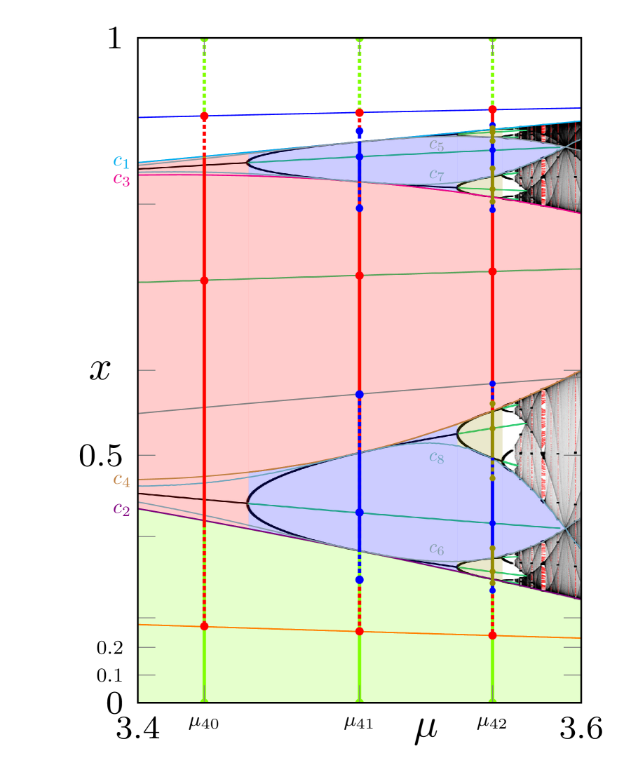
Figure 6: Examples of $U_{k}$ sets in case of flip trapping regions. This picture is discussed in detail in Sec. 4.7.

Example 7.

Consider the case, shown in Fig. 6, of the logistic map $f$ with $\mu=\mu_{40}$. This map has three nodes: $N_{1}$ is the fixed point other than $x=0$ and the attractor $N_{2}$ is a 2-cycle $\{p^{\prime}_{1},p^{\prime}_{2}\}$. In this case

$$U_{2}=\{p^{\prime}_{1},p^{\prime}_{2}\},\;U_{1}=[c_{2},p^{\prime}_{1})\cup(p^{\prime}_{1},p^{\prime}_{2})\cup(p^{\prime}_{2},c_{1}].$$

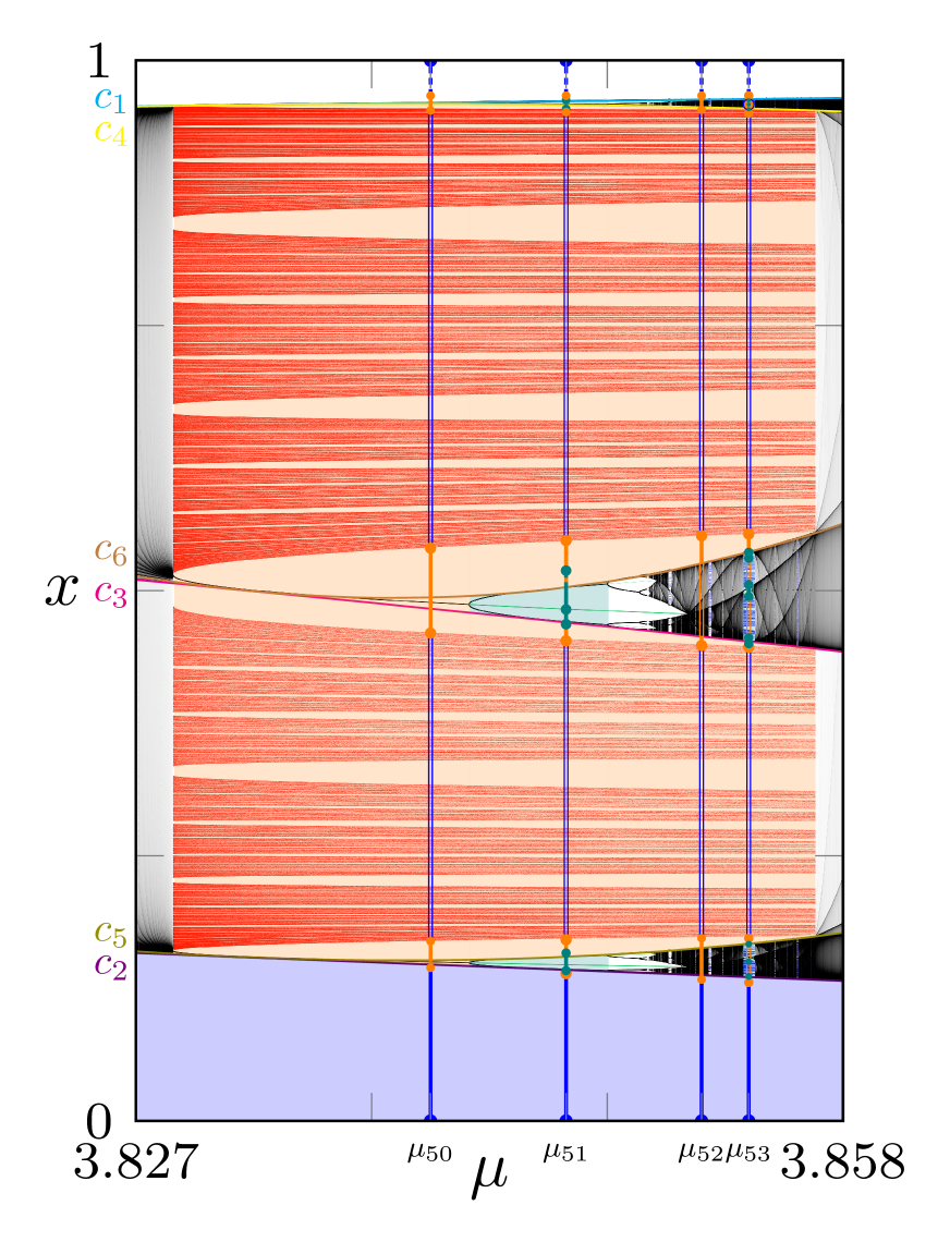
Figure 7: Examples of $U_{k}$ sets in case of regular trapping regions. This picture is discussed in detail in Sec. 4.7.

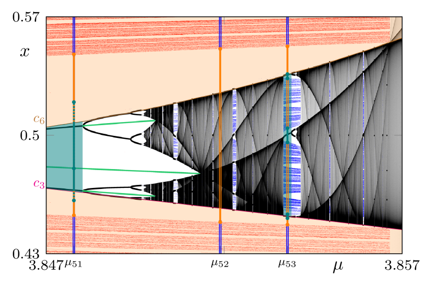
Figure 8: Close-up of the central cascade in Fig. 7. This picture is discussed in detail in Sec. 4.7.

Example 8.

Consider the case, shown in Fig. 7, of the logistic map with $\mu=\mu_{53}$. This map has four nodes: $N_{1}$ is a Cantor set, painted in red; $N_{2}$ is a second Cantor set, painted in blue; the attractor $N_{3}$, three points of which are visible (in black) in Fig. 8, is a 9-cycle. In this case,

$$U_{3}=N_{3},\;U_{2}=[c_{2},c_{5}]\cup[c_{3},c_{6}]\cup[c_{4},c_{1}]\setminus N_{3},\;U_{1}=(c_{5},c_{3})\cup(c_{6},c_{5}).$$

4.1 Forward limits.

While the focus of this article is on backward limits, for completeness we include also the following result about the relation between the forward limit of a point and its position.

Theorem 1 ($\bm{\omega}$-limits of S-unimodal maps.).

Assume that $f$ satisfies (A) and let $x\in U_{k}$. Then $\omega_{f}(x)\subset N_{i}$ for some unique $i\geq k$.

Proof.

By the Chain-Recurrent Spectral Theorem, we know the following:

1. Trapping regions are nested one into the other and are all forward invariant;

2. $N_{j}\subset J^{int}(N_{k})$ for all $j>k$;

3. $N_{j}\cap J^{int}(N_{k})=\emptyset$ for all $j\leq k$;

4. $N_{k}\cap\overline{J^{int}(N_{k})}$ is a single periodic orbit.

Hence, the $\omega$-limit set of any $x$ which lies into $U_{k}$ must be contained in one of the nodes $N_{i}$ for some $i=k,\dots,p$. ∎

In particular, this means that the set of possible outcomes for $\omega_{f}(x)$ is a locally constant monotonically decreasing function of the distance of $x$ from the critical point $c$.

Remark 3.

By Theorem B, $\omega(x)$ must be either a cycle or a Cantor set or an interval cycle. Moreover, for Lebesgue-almost all $x$, $\omega(x)=N_{p}$ [16, 17]. Since all other nodes are repelling, when $\omega(x)\subset N_{i}$ for some $i\neq p$ the only possibility is that there is a forward trajectory starting at $x$ that actually falls on $N_{i}$ in a finite number of iterations. Equivalently, such $x$ must belong to a backward trajectory from some point in $N_{i}$.

We turn now to the main goal of this article, which is studying the possible $s\alpha$-limits of a point depending on its level, namely depending on which $U_{k}$ set it belongs to. Following Conley’s observation that points either belong to some node or are gradient-like, we discuss separately these two cases. All these partial results will be finally summarized in Thm. 5 (Sec. 4.6).

4.2 Backward limits within repelling nodes.

As we recalled earlier, repelling nodes are either cycles (type $R_{1}$) or transitive (see Def. 20) Cantor sets (type $R_{2}$). The restriction of $f$ to either case is topologically conjugated to a subshift of finite type, a fact that was proved first by van Strien in 1981 [41] using kneading theory. For sake of clarity and self-completeness, we sketch below a more explicit proof of this fact that will also lead us to establish that $s\alpha_{f}(x)\supset N$ for each point $x$ belonging to a repelling node $N$.

The case of node $N_{1}$ in the period-3 window of $\bm{\ell_{\mu}}$. Consider the concrete case of the period-3 window $W$ of the logistic map $f=\ell_{\mu}$ (see Figs. 1 and  7). For every $\mu$ in the interior of $W$, the point $p_{1}(N_{1})$ belongs to a repelling 3-cycle and ${\mathcal{T}}(N_{1})=\{J_{1},J_{2},J_{3}\}$ is a regular period-3 trapping region. Since the $J_{i}$ are disjoint, the set $C=[0,1]\setminus\cup_{k=0}^{\infty}f^{-k}(J_{1})$ of all points that do not ever fall in $J_{1}$ is the complement of a dense countably infinite union of disjoint intervals and so is a Cantor set (see Prop. 3.21 in [11] for more details).

Decomposing $\bm{C}$. Recall that, when $\bar{p}>c$, each node different from $N_{0}$ lies inside $[f^{2}(c),f(c)]$ and that, since $c$ belongs to either the basin of the attractor or to the attractor itself, each repelling node actually lies in $L_{c}=(f^{2}(c),f(c))$. Hence $N_{1}\subset C\cap L_{c}$. Furthermore, by construction we have that

$$N_{1}\subset C\cap\left(L_{c}\setminus J^{int}(N_{1})\right).$$

The set $L_{c}\setminus J^{int}(N_{1})$ is the disjoint union of the two closed intervals

$$A_{0}=[p_{3},1-p_{1}]\hbox{ and }A_{1}=[p_{1},p_{2}]$$

and so, correspondingly, we can write

$$C\cap L_{c}=C_{0}\sqcup C_{1},$$

with $C_{i}=C\cap A_{i}$, $i=0,1$.

A map $\bm{s:C_{0}\sqcup C_{1}\to\Sigma_{2}}$. Exploiting the decomposition above, one can associate to the trajectory $\{f^{n}(p)\}$ of each point $p\in C\cap L_{c}$ an element $s(p)=(s_{0},s_{1},\dots)$ of the single-sided shift space $\Sigma_{2}$ in two symbols, say 0 and 1, so that $s_{n}=0$ if $f^{n}(p)\in C_{0}$ and $s_{n}=1$ otherwise.

For instance, for every $\mu\in W$, the map $f$ has a fixed point $\bar{p}$ inside $C_{1}$, so

$$s(\bar{p})=(111\dots).$$

Since $f^{2}$ is a polynomial of degree 4 and both fixed points of $f$ are also fixed points of $f^{2}$, for every $\mu\in W$ the map $f$ has a single 2-cycle $\{\bar{q}_{1},\bar{q}_{2}\}$, $\bar{q}_{1}<\bar{q}_{2}$. Note that it is impossible that $\bar{q}_{2}<c$ since $f(\bar{q}_{1})=\bar{q}_{2}$ would imply $f(\bar{q}_{2})>\bar{q}_{2}$. Moreover, since within $W$ this 2-cycle is repelling, then necessarily $f^{2}(c)<c$ and so $c\in(\bar{q}_{1},\bar{q}_{2})$. Hence,

$$s(\bar{q}_{1})=(0101\dots),\;\;s(f(\bar{q}_{1}))=s(\bar{q}_{2})=(1010\dots).$$

Finally, in case of the 3-cycle $\Gamma(N_{1})$, we have that

$$s(p_{1}(N_{1}))=(110110\dots),\;s(f(p_{1}(N_{1})))=s(p_{2})=(101101\dots),\;s(f^{2}(p_{1}(N_{1})))=s(p_{3})=(011011\dots).$$

Notice that, by construction,

$$s(f(p))=\sigma(s(p)),$$

where $\sigma:\Sigma_{2}\to\Sigma_{2}$ is the standard shift operator $\sigma((a_{1}a_{2}a_{3}\dots))=(a_{2}a_{3}\dots)$.

Each $\bm{s(p)}$ misses the word “00”… While $(111\dots)$ is in the range of $s$, $(000\dots)$ is not, since the other fixed point of $f$, namely the node $N_{0}$, does not belong to $N_{1}$. This is an example of the following more general property: $\sigma(p)$ cannot contain the word “00”. Indeed, since $[p_{3},1-p_{1}]\subset[0,c]$,

$$f(A_{0})=f([p_{3},1-p_{1}])=[f(p_{3}),f(1-p_{1})]=[p_{1},p_{2}]=A_{1}$$

while, since $[p_{1},p_{2}]\subset[c,1]$,

$$f(A_{1})=f([p_{1},p_{2}])=[f(p_{2}),f(p_{1})]=[p_{3},p_{2}]=A_{0}\cup J_{1}(N_{1})\cup A_{1}.$$

Since $C\cap L_{c}$ is invariant under $f$, this means ultimately that

$$f(C_{0})\subset C_{1},\;f(C_{1})\subset C_{0}\sqcup C_{1}.$$

In particular, if the $n$-th component of $s(p)$ is 0, then its $(n+1)$-th component must be 1.

…but misses no other word. Denote by $W_{00}$ the subset of $\Sigma_{2}$ of all elements not containing the word “00”. Clearly $W_{00}$ is a subshift of finite type, namely it is invariant under $\sigma$ and is defined by a finite number of conditions (in fact, by just one condition). We claim that, for each element $w=W_{00}$, there is $p\in C\cap L_{c}$ such that $s(p)=w$.

Indeed, let $w=(w_{1}w_{2}w_{3}\dots)$ and define the following sets:

$$I_{w,1} = A_{w_{1}}$$

$$I_{w,2} = A_{w_{1}}\cap f^{-1}(A_{w_{2}})$$

$$I_{w,3} = A_{w_{1}}\cap f^{-1}(A_{w_{2}})\cap f^{-2}(A_{w_{3}})=A_{w_{1}}\cap f^{-1}(A_{w_{2}}\cap f^{-1}(A_{w_{3}}))$$

$$I_{w,4} = A_{w_{1}}\cap f^{-1}(A_{w_{2}})\cap f^{-2}(A_{w_{3}})\cap f^{-3}(A_{w_{4}})=A_{w_{1}}\cap f^{-1}(A_{w_{2}}\cap f^{-1}(A_{w_{3}}\cap f^{-1}(A_{w_{4}})))$$

$$\dots$$

By construction, $I_{w,k}$ is the open subset of $C$ containing all points whose first $k$ symbols coincide with the first $k$ symbols of $w$. Set $I_{w}=\cap_{k=1}^{\infty}I_{w,k}$. Then $I_{w}\subset C_{0}\sqcup C_{1}$ since the orbit of any point of $I_{w}$ never leaves $A_{0}\sqcup A_{1}$ and $s(p)=w$ for every $p\in I_{w}$.

In order to show that $I_{w}$ is non-empty for each $w\in W_{00}$, we point out that, since $f$ is unimodal, the counterimage of any interval not containing $c$ is the union of two intervals lying on opposite side with respect to $c$. Given the action of $f$ on $A_{0}$ and $A_{1}$, we furthermore have that the counterimage under $f|_{A_{0}\sqcup A_{1}}$ of any interval in $A_{0}$ is a subinterval of $A_{1}$ while the counterimage of any interval in $A_{1}$ is a pair of intervals, one in $A_{0}$ and one in $A_{1}$. Hence, from the expression of $I_{w,k}$, it is clear that this set is empty if and only if, for some $r\leq k$, the interval $A_{w_{r}}\cap f^{-1}(\dots)$ lies in $A_{0}$ (so $w_{r}=0$) and, at the following step $A_{w_{r-1}}\cap f^{-1}(A_{w_{r}}\cap f^{-1}(\dots))$, we have $A_{w_{r-1}}=A_{0}$ (namely $w_{r-1}=0$). Ultimately, this argument shows that $I_{w}$ is empty if and only if $w$ contains the word “00”.

$\bm{s}$ is injective. Since $I_{w}\subset C_{0}\sqcup C_{1}$ is a closed interval and $C_{0}\sqcup C_{1}$ is a Cantor set, the only possibility is that $I_{w}$ is a single point, namely $s:C_{0}\sqcup C_{1}\to W_{00}$ is a bijection.

$\bm{s}$ is a homeomorphism. A basic neighborhood $U_{w}$ of a point $w_{0}\in W_{00}$ is the set of all $w\in W_{00}$ that coincide with $w_{0}$ up to their $r$-th component for some $r>0$. The set $s^{-1}(U_{w})$ is the set we denoted above by $I_{w,r}$ and, as we pointed out above, this is always a neighborhood of $s^{-1}(w)$. Similarly, due to the continuity of $f$, given any $p\in C_{0}\sqcup C_{1}$, for each $M>0$ there is a neighborhood $V_{p}$ of $p$ such that $s(p)$ and $s(p^{\prime})$ coincide up to their first $M$ symbols for each $p^{\prime}\in V_{p}$

$\bm{f|_{N_{1}}}$ is topologically conjugated to $\bm{\sigma}$. This is an immediate consequence of the fact that, as pointed out above, $s\circ f=\sigma\circ s$ for all points of $N_{1}$ and that $s$ is a homeomorphism.

$\bm{N_{1}=C\cap L_{c}}$. Because of the points above, it is enough to show that there is an $\varepsilon$-chain between every two points of $s(C\cap L_{c})$. Given $x,y\in s(C\cap L_{c})$ and $\varepsilon>0$, there is an element $z$ whose distance from $x$ is smaller than $\varepsilon$ so that all components $z_{i}$ up to some finite index $n=n(\varepsilon)>0$ coincide with the components $x_{i}$ while $z_{n+i}=y_{i}$ for all $i>0$. Then the sequence

$$x,z,\sigma(z),\dots,\sigma^{n}(z)=y$$

is an $\varepsilon$-chain between $x$ and $y$.

Hence, $N_{1}$ is the set of all points in $[f^{2}(c),f(c)]$ that do not fall into $J^{int}(N_{1})$ under $f$.

The general case. Consider the general case of a Cantor set retractor $N_{k}$. Denote by $r$ the period of the trapping region ${\mathcal{T}}(N_{k-1})$ and set $\bar{f}_{i}=f^{r}|_{J_{i}(N_{k-1})}$. Then each $\bar{f}_{i}:J_{i}(N_{k-1})\to J_{i}(N_{k-1})$ is a S-unimodal map having first node $\overline{N}_{i,0}=\{p_{i}(N_{k-1})\}$ and second node the repelling Cantor set $\overline{N}_{i,1}=N_{k}\cap J_{i}(N_{k-1})$. Note that $|{\mathcal{T}}(\overline{N}_{i,1})|=|{\mathcal{T}}(N_{k})|/|{\mathcal{T}}(N_{k-1})|,\;i=1,\dots,r.$

Similarly to the case above, $\overline{N}_{i,1}\subset[c_{2r-i-1},c_{r-i-1}]$ and the set $(c_{2r-i-1},c_{r-i-1})\setminus J^{int}(\overline{N}_{i,1})$ is the disjoint union of $r-2$ closed intervals $A_{i,1},\dots,A_{i,r-2}$. Hence, like we did above, we can associate to each point $p\in(c_{2r-i-1},c_{r-i-1})\setminus\cup_{k=0}^{\infty}\bar{f}_{i}^{-k}(J_{1}(\overline{N}_{i,1}))$ an element $\sigma_{i}(p)$ belonging to the single-sided shift space $\Sigma_{r-2}$. Correspondingly to the action of $\bar{f}_{i}$ on the $A_{i,k}$, there will be some number of words that will not appear in any $\sigma_{i}(p)$. Since there is a finite number of $A_{i,k}$, there will be a finite number of forbidden words. Similarly to how we did above, one can prove that these maps $\sigma_{i}$ are continuous and injective and all elements of $\Sigma_{r-2}$ without those forbidden words in their sequence are the image of some $p$. Hence, the image of each $\sigma_{i}$ is a subshift of finite type.

Ultimately, we illustrated the following result:

Theorem K ([41]).

Let $N$ be a repelling node of a S-unimodal map $f$. Then $f|_{N}$ is topologically conjugate to a subshift of finite type.

4.3 Backward dense orbits in subshifts of finite type.

Shifts have been thoroughly studied because they appear ubiquitously in every dynamics subfield. Nevertheless the following elementary result on backward dynamics, in the author’s knowledge, did not appear explicitly so far in literature.

Theorem 2.

Let $S$ be a 1-sided subshift of finite type with a dense trajectory. Then each point has a backward dense bitrajectory.

Proof.

Let $F$ be the full 2-sided shift in the same symbols $\alpha_{1},\dots\alpha_{k}$ of $S$. A bitrajectory passing through an element $x=(x_{1}x_{2}x_{3}\dots)\in S$ is an element $X=(\dots x_{-3}x_{-2}x_{-1}\,.\,x_{1}x_{2}x_{3}\dots)\in F$.

Recall that, in a (1- or 2-sided) shift space $X$ with a dense trajectory, for any two words $w,w^{\prime}\in X$, there is a word $u\in X$ such that $wuw^{\prime}\in X$ [5]. Since in $S$ there is an element $d=(d_{1}d_{2}d_{3}\dots)$ with a dense trajectory, the same is true about $F$: given any element $Y=(\dots y_{-3}y_{-2}y_{-1}\,.\,y_{1}y_{2}y_{3}\dots)$ there is some finite word $u_{1}\dots u_{r}$ such that

$$D=(\dots y_{-3}y_{-2}y_{-1}u_{1}\dots u_{r}\,.\,d_{1}d_{2}d_{3}\dots)\in F.$$

By Sec. 9.1 in [26], every irreducible 2-sided shift (namely a 2-sided shift with a dense trajectory) has a doubly transitive point $T=(\dots t_{-3}t_{-2}t_{-1}\,.\,t_{1}t_{2}t_{3}\dots)$, namely a point whose orbit is dense both backward and forward.

Now, given any $x=(x_{1}x_{2}x_{3}\dots)\in S$, there is a finite word $u_{1}\dots u_{s}$ such that $X=(\dots t_{-3}t_{-2}t_{-1}u_{1}\dots u_{s}\,.\,x_{1}x_{2}x_{3}\dots)\in F$. This point represents precisely a bitrajectory passing through $x$ whose backward orbit is dense by construction. ∎

As a corollary, we obtain our main result on retractors.

Theorem 3.

Every point of a repelling node $N$ of $f$ has a bitrajectory backward dense in $N$.

4.4 Backward limits within attracting nodes.

Of the five types of attracting nodes, only types $A_{2}$ and $A_{5}$, namely the two cases when the attractor is chaotic, are non-trivial. Indeed, cases $A_{1}$ (stable periodic orbit) and $A_{4}$ (single-sided stable periodic orbit belonging to a Cantor repellor) are covered by the results of the previous subsection. About case $A_{3}$, we recall that it is well-known that, in a minimal set, every point has a dense backward orbit [25].

Backward orbits in a chaotic attractor. Let $A$ be a chaotic attractor, namely an attracting trapping region. Recall that in $A$, as well as in every retracting node, there is a dense set of periodic points (but $c$ does not belong to any of them, since any cycle containing $c$ is superattracting). In each retractor node $N_{k}$ we have a special cycle, the minimal cycle $\Gamma(N_{k})$, which is the cycle passing through $p_{1}(N_{k})$, the closest point of $N_{k}$ to $c$. On the contrary, none of the cycles within $A$ can be minimal, since $A$ belongs to the attracting node and nodes are disjoint. Nevertheless, in analogy with minimal cycles, we give the following standard definition.

Definition 18.

Given $p,q\in[a,b]$, we say that $p$ is closer to $\bm{c}$ than $q$ if $(p,\hat{p})\subset(q,\hat{q})$, where as usual $\hat{p}$ is the root of $f(x)=f(p)$ other than $p$. Given a cycle $\gamma$, we denote by $p_{1}(\gamma)$ the point of $\gamma$ that is the closest to $c$ and we set $J_{1}(\gamma)=[p_{1}(\gamma),\hat{p}_{1}(\gamma)]$. We say that the cycle $\gamma$ is closer to $c$ than the cycle $\gamma^{\prime}$ when $p_{1}(\gamma)$ is closer to $c$ than $p_{1}(\gamma^{\prime})$.

Remark 4.

The relation among cycles given by “being closer to $c$” is a linear order in the set of all cycles of $f$. In case of the logistic map, the distance between $p_{1}(\gamma)$ and $c$ is the same as between $\hat{p}_{1}(\gamma)=1-p_{1}(\gamma)$ and $c$ and so the “being closer” relation in this case is literal.

Minimal cycles are quite special: either there are only finitely many of them (when $N_{p}$ is not of type $A_{3}$) or $p_{1}(\Gamma(N_{k}))\to c$ (otherwise). On the contrary, the set of accumulation points of the set of all points $p_{1}(\gamma)$ of all cycles $\gamma$ of a S-unimodal map $f$ having at least one repelling Cantor set is large (easy to build examples in subshifts of finite type). Next definition highlights a type of cycle which represents a slight generalization minimal ones and is of central importance in the chaotic case.

Definition 19 ([16]).

Given a regular (resp. flip) $n$-cycle $\gamma\subset A$, we say that $p_{1}(\gamma)$ is regular central (resp. flip central) if $f^{n}$ (resp. $f^{2n}$) is monotonic on $(p_{1}(\gamma),c)$, namely if $c\not\in f^{i}(J_{1}(\gamma))$ for $i=1,\dots,n-1$ (resp. $i=1,\dots,2n-1$). When $p_{1}(\gamma)$ is central, we also say that $\gamma$ itself is central. Finally, we say that a closed interval $H$ is a homterval for $f$ if $c\not\in f^{k}(H)$ for any integer $k\geq 0$, namely if all iterates $f^{k}$, $k=0,1,\dots$, are strictly monotonic on $H$.

Example 9.

Every minimal cycle $\Gamma({\mathcal{T}})$ is central and its point $p_{1}({\mathcal{T}})$ is a central point.

Example 10.

Consider the unique 2-cycle $\gamma_{2}=\{q_{-},q_{+}\}$ of the logistic map. For each $\mu\in[1+\sqrt{5},4]$, $\gamma_{2}$ is flip. For $\mu\in[1+\sqrt{5},\mu_{MF}]$, where $\mu_{MF}$ is the Myrberg-Feigenbaum point, $\gamma_{2}$ is a node. Hence, close enough from the right to $\mu_{MF}$, $\gamma_{2}$ is a flip central point. On the other side, at $\mu=4$ we have that $q_{\pm}=\frac{5\pm\sqrt{5}}{8}$, so that $q_{-}<c<q_{+}$ and $q_{-}$ is the closest to $c$. Set $J_{1}=[q_{-},1-q_{-}]$. Hence

$$f(J_{1})=[q_{+},1],\;f^{2}(J_{1})=f([q_{+},1])=[0,q_{-}],\;f^{3}(J_{1})=f([0,q_{-}])=[0,q_{+}]$$

Since $c\in f^{3}(J_{1})$, $\gamma_{2}$ is not central. For $\mu$ close enough to 4 from the left, $c_{1}$ is close to 1 and both $c_{2}$ and $c_{3}$ are close to 0, so that still $c\in f^{3}(J_{1})$.

Proposition 7.

Let $f$ be a S-unimodal map and $\bar{p}$ its internal fixed point. There is no flip cycle if $\bar{p}\leq c$. For $c<\bar{p}$, the lowest-period flip central point of $f$ is $\bar{p}$. If $f$ has a regular 3-cycle $\gamma$, then $p_{1}(\gamma)$ is the lowest-period regular central point of $f$.

Proof.

Set $\bar{J}_{1}=[\hat{\bar{p}},\bar{p}]$. Then $f(J_{1})=[\bar{p},c_{1}]$, which does not contain $c$, and so $\bar{p}$ is flip central. Consider now the case when $f$ has a regular 3-cycle $\{p_{1},p_{2},p_{3}\}$. Set $J_{1}=[\hat{p}_{1},p_{1}]$. Then $f(J_{1})=[p_{2},c_{1}]$ and $f^{2}(J_{1})=[c_{2},p_{3}]$. Clearly $c$ does not belong to either one of these two sets and so $p_{1}$ is central. ∎

The following facts are crucial for our results below:

Theorem L ([16]).

Let $f$ have a chaotic attractor $A=N_{p}$ and set $r=|{\mathcal{T}}(N_{p-1})|$. Then:

1. $c\in A$;

2. $\alpha_{f}(c)=[a,b]$;

3. for any neighborhood $U$ of the critical point, there is a central cycle $\gamma$ with $J_{1}(\gamma)\subset U$;

4. for each central $s$-cycle $\gamma\subset A$, with $s>r$ if $\gamma$ is regular and $2s>r$ if it is flip, there is a central cycle $\gamma^{\prime}\subset A$, closer to $c$ than $\gamma$, and a $k>0$ such that $f^{k}(J_{1}(\gamma^{\prime}))\supset J_{1}(\gamma)$;

5. $f$ has no homtervals.

The following proposition is implicitly used in a proof in [16] (see also Thm. II.7.9 in [6]).

Proposition 8.

The set $C_{f}$ of all central points of a S-unimodal map $f$ is finite if and only if $N_{p}$ is of type $A_{1}$ or $A_{4}$. When $C_{f}$ is infinite, the only point of accumulation of the set of all central points of $f$ is the critical point.

Proof.

Suppose first that there are infinitely many central points. Consider a sequence $q_{k}$ of central points of period $n_{k}$ such that $q_{k}$ is closer to $c$ than $q_{k-1}$ for all $k$ and suppose that $q_{k}\to q_{\infty}\neq c$. Then there is some closed non-trivial interval $H\subset(q_{\infty},1-q_{\infty})$ not containing the critical point. Now, notice that $n_{k}\to\infty$ because there is a finite number of cycles of any given period. Hence $c\not\in f^{n}(H)$ for any $n\geq 0$ since, for any given $n$, there are $k$ for which $n_{k}>n$ and for such $k$ we must have that $c\not\in f^{i}(q_{k},1-q_{k})$ for $i=1,\dots,n_{k}-1$. So $H$ is a homterval, which contradicts point (5) of the theorem above.

By point (3) of the previous theorem, when the attractor is chaotic (namely $N_{p}$ is of type $A_{2}$ or $A_{5}$) there are infinitely many central points. When $N_{p}$ is of type $A_{3}$, there are infinitely many nodes $N_{k}$ and each point $p_{1}({\mathcal{T}}(N_{k}))$ is central. When the attractor is a cycle $\gamma$ (namely $N_{p}$ is of type $A_{1}$ or $A_{4}$), then $\gamma$ is minimal and the interval $J^{1}(\gamma)$ is contained in the basin of attraction of $\gamma$ and so cannot contain any point belonging to a cycle. ∎

The case $\bm{N_{1}=A}$. In this case there are only two nodes, the fixed endpoint $N_{0}$ and the chaotic attractor $N_{1}=A$, which is of type $A_{2}$. The chaotic attractor must consist into a single interval, since the non-internal fixed point $\bar{p}$ of $f$ must belong to it (or there would be a third node) and a trapping region with more than one component cannot contain any fixed point. Since $c\in A$, then $A=[c_{2},c_{1}]$.

The general case. In case $p>1$, set $r=|{\mathcal{T}}(N_{p-1})|$. Then the $J_{i}(N_{p-1})$ are invariant under $f^{r}$ and we set $\bar{f}_{i}=f^{r}|_{J_{i}(N_{p-1})}$. Then each $\bar{f}_{i}$ has just two nodes: the repelling fixed point $p_{i}(N_{p-1})$ and the chaotic attractor $N_{p}\cap J_{i}(N_{p-1})=[c_{2r-i-1},c_{r-i-1}]$. Hence, we reduce again the the previous case.

In order to prove the existence of backward dense orbits, we use the two general results below about topological dynamical systems.

Definition 20 ([3]).

A dynamical system $f:X\to X$ is transitive if it has a dense orbit.

Several properties equivalent to topological transitivity can be found in [24].

Theorem M ([28]).

Each transitive map $f$ has a dense set of points with a backward dense orbit.

Definition 21 ([34]).

A dynamical system $f:X\to X$ is very strongly transitive if, for every open set $U\subset X$, there is a $n\geq 1$ such that $\cup_{i=1}^{n}f^{i}(U)=X$.

Recently Akin, Auslander and Nagar gave the following characterization of very strongly transitive systems.

Theorem N ([1]).

A dynamical system $f:X\to X$ is very strongly transitive if and only if for any $x\in X$ and $\varepsilon>0$ there is a $N>0$ such that $A_{N}(x)=\bigcup_{i=1}^{N}f^{-i}(x)$ is $\varepsilon$-dense, namely $A_{N}(x)$ intersect all balls of radius $\varepsilon$ in $X$.

Proposition 9.

The restriction of $f$ to $N_{p}=A$ is very strongly transitive.

Proof.

The general case argument above shows that it is enough to consider the case $p=1$. Since $c$ has a dense set of counterimages in $A$ and there are central cycles arbitrarily close to $c$, we can assume without loss of generality that $U=int(J_{1}(\gamma))$ for some central cycle $\gamma$.

As shown in Prop. 7, the fixed point $\bar{p}$ is a flip central point for $f$. Set $\bar{J}_{1}=[\hat{\bar{p}},\bar{p}]$. Then we have that $f(\bar{J}_{1})=[\bar{p},c_{1}]$ and $f^{2}(\bar{J}_{1})=[c_{2},\bar{p}]$, so that

$$A=f(\bar{J}_{1})\cup f^{2}(\bar{J}_{1}),\;\;f(\bar{J}_{1})\cap f^{2}(\bar{J}_{1})=\{\bar{p}\}.$$

Starting from the central cycle $\gamma_{0}=\{\bar{p}\}$, we can build a sequence of central cycles $\gamma_{k}$ so that, for each $k\geq 1$, $J_{1}(\gamma_{k})\subset J_{1}(\gamma_{k-1})$ and there is a $n_{k}\geq 2$ such that $f^{n_{k}}(J_{1}(\gamma_{k}))\supset J_{1}(\gamma_{k-1})$. In particular, for each $k\geq 1$ there is a $N_{k}$ such that $f^{N_{k}}(J_{1}(\gamma_{k}))\supset J_{1}(\gamma_{0})$. Since, by Proposition 8, central points can only accumulate at $c$, then $\lim_{k\to\infty}p_{1}(\gamma_{k})=c$ and so there is some $r\geq 1$ such that $\gamma_{r}$ is closer to $c$ than $\gamma$ and so $f^{n_{r}}(J_{1}(\gamma))\supset J_{1}(\gamma_{0}).$ Hence $f^{n_{r}+1}(J_{1}(\gamma))\supset[\bar{p},c_{1}]$ and $f^{n_{r}+2}(J_{1}(\gamma))\supset[c_{2},\bar{p}]$, namely $\bigcup_{i=1}^{n_{r}+2}f^{i}(J_{1}(\gamma))=A.$ ∎

Now we are ready to prove our main result on chaotic attractors.

Theorem 4.

Every point of a chaotic attractor $A$ of $f$ has a bitrajectory backward dense in $A$. In particular, every point of an attracting node $N$ of type $A_{2}$ has a backward orbit dense in $N$.

Proof.

By Thm. M applied to the restriction of $f$ to $A$, there are points in $A$ having a backward orbit dense in $A$. Let $b=(b_{1},b_{2},...)$ be one of these backward dense orbits and let $x_{0}$ be any point of $A$. Let $x_{1}$ be a counterimage of $x_{0}$ of some order $n_{1}\geq 0$ closer to $b_{1}$ than $1/1$. Such counterimage exists by Thm. N. Then let $x_{2}$ be a counterimage of $x_{1}$ of some order $n_{2}\geq 0$ closer to $b_{2}$ than $1/2$ and so on. All these counterimages exist by Thm. N. The backward orbit $(x_{0},x_{1},x_{2},\dots)$ is easily seen to be dense as well. ∎

The case of nodes of type $A_{5}$. As we pointed out in Remark 2, a node of type $A_{5}$ contains, besides a chaotic attractor which is also a cyclic trapping region, the following two sets: 1) a repelling Cantor set, with which it shares a cycle, and 2) intervals of points that are not non-wandering. Since no backward trajectory can asymptote to points that are not non-wandering, in this case no point has a bitrajectory which is backward dense in the whole node.

4.5 Backward limits of non-chain-recurrent points.

As pointed out initially by Conley in the continuous finite-dimensional case, and extended later by Norton to the discrete case [33], all bitrajectories through non-chain-recurrent points have their backward and forward limits belonging to different nodes, so that they determine an edge of the graph. Below we present two examples that turn out to be typical.

Backward limits of level-0,1 points when $N_{1}$ is a repelling cycle. This happens, for instance, in case of the logistic map $f=\ell_{\mu}$ for $\mu\in(3,\mu_{M})$. We already discussed in Example 5 the structure of the sets $U_{k}$.

Points in $U_{-1}$ have no counterimage, so $s\alpha_{f}(x)=\emptyset$ if $x\in U_{-1}$.

Each $x\in U_{0}$ has two counterimages but one of them lies in $U_{-1}$, so there is a single bitrajectory passing through each such $x$. Since $x=0$ is backward attracting, this bitrajectory asymptotes backward to 0. Hence, $s\alpha_{f}(x)=N_{0}$ if $x\in U_{0}$.

More generally, each point in $[0,c_{1}]$ has a backward trajectory asymptoting to $0$ since any interval $[0,\varepsilon]$, $\varepsilon>0$, will eventually cover the whole image of $f$ under iterations, so $s\alpha_{f}(x)\supset N_{0}$ if $x\in[0,c_{1}]$. Indeed, recall that an interval not containing $c$ such that none of its iterates contain $c$ is called a homterval (see [11] for more details on homtervals and on the argument below). As a consequence of a fundamental result of Guckenheimer [16], the only configuration when a homterval can arise in a S-unimodal map is when the attractor $N_{p}$ is a cycle and the node $N_{p-1}$ is also a cycle. In that case, the interval between a point $x\in N_{p}$ and a point $y\in N_{p-1}$ such that no other node point lies in $[x,y]$ is a homterval. No other type of homterval can arise. This means that, in all possible cases, under iterations $[0,\varepsilon]$ will eventually cover $c$ and so, in the following step, will cover all points in the image of the map.

Now consider the period-2 cyclic trapping region of $N_{1}$, namely the two intervals

$$J_{1}(N_{1})=[q_{1},p_{1}],J_{2}(N_{1})=[p_{1},q_{2}]$$

where $q_{1}=\hat{p}_{1}$ and $f(q_{2})=q_{1}$. Notice that both $J_{1}$ and $J_{2}$ are forward invariant under $\bar{f}=f^{2}$ and let us set $g=f|_{J_{2}}$. Since $c\not\in J_{2}$, the map $g:J_{2}\to J_{1}$ is a diffeomorphism. For the same reasons above, within $J_{1}$ only points in $[\bar{f}(c),p_{1}]=[c_{2},p_{1}]$ have a backward trajectory asymptoting to $p_{1}$. Hence, in $J_{2}$, only points in $[g^{-1}(c_{2}),g^{-1}(p_{1})]=[p_{1},c_{1}]$ have a backward trajectory asymptoting to $p_{1}$. This means ultimately that the only points with backward trajectories asymptoting to $p_{1}$ are the points in the interval $[c_{2},c_{1}]$. Since $U_{1}\subset[c_{2},c_{1}]$, we have that $s\alpha_{f}(x)=N_{0}\cup N_{1}$ if $x\in U_{1}$.

Backward limits of level-0,1 points when $N_{1}$ is a repelling Cantor set. This happens, for instance, in case of the logistic map $f=\ell_{\mu}$ for $\mu\in(1+2\sqrt{2},3.868\dots)$. We already discussed in Example 6 the structure of the sets $U_{k}$.

Just like the case above, points in $U_{-1}$ have no bitrajectories passing through them and all points in $[0,c_{1}]$ have a backward trajectory asymptoting to $0$.

As discussed in Sec. 4.2, the Cantor set $N_{1}$ is the set of all chain-recurrent points in $[c_{2},c_{1}]$ that do not lie in $J^{int}(N_{1})$. Each point $x\in[c_{2},c_{1}]$ is either a point of $N_{1}$ or lies in a counterimage of $J_{1}(N_{1})$. The case of points of $N_{1}$ has been discussed in Sec. 4.2. In the other case, since by definition $N_{1}=[c_{2},c_{1}]\setminus\cup_{k\geq 0}f^{-k}(J_{1}(N_{1}))$, every point in $[c_{2},c_{1}]\setminus N_{1}$ belongs to a backward trajectory starting in the interior of $J_{1}(N_{1})$ and asymptoting to $N_{1}$. In any case, then, $s\alpha_{f}(x)=N_{0}\cup N_{1}$ if $x\in U_{1}$.

4.6 Main theorem.

We are now ready to prove the main result of the article.

Theorem 5 ($\bm{s\alpha}$-limits of S-unimodal maps).

Assume that $f$ satisfy (A). If $x$ is a level-$k$ point, $k<p$, then $s\alpha_{f}(x)=\bigcup\limits_{i=0}^{k}N_{i}$. If $k=p$ and $N_{p}$ is not of type $A_{5}$, then $s\alpha_{f}(x)=\bigcup\limits_{i=0}^{p}N_{i}=\Omega_{f}$ for all level-$p$ points. If $N_{p}$ is of type $A_{5}$, denote by $C$ and $A$ respectively the repelling Cantor set and the attractor contained in $N_{p}$. Then $s\alpha_{f}(x)=\Omega_{f}$ if $x\in A$ and $s\alpha_{f}(x)=\bigcup\limits_{i=0}^{p-1}N_{i}\cup C=\Omega_{f}\setminus int(A)$ otherwise.

Proof.

We start by pointing out that, for $k=0,\dots,p-1$, $K(N_{k})$ is the set of all points of $\overline{J^{int}(N_{k})}$ that have a backward trajectory asymptoting to $N_{k+1}$. Indeed, let $r$ be the period of ${\mathcal{T}}(N_{k})$ and set $\bar{f}=f^{r}$. Then each $J_{i}(N_{k})$ is forward-invariant under $\bar{f}$ and after restricting $\bar{f}$ to each of the $J_{i}(N_{k})$ we reduce to either one of the two case examples in Section 4.5.

Since $K(N_{k})\subset K(N_{k^{\prime}})$ for $k^{\prime}\leq k$, then every point of $K(N_{k})$ has also a backward trajectory asymptoting to $N_{k^{\prime}+1}$ for $k^{\prime}\leq k$. Since $U_{k}\subset K(N_{k-1})$, then $s\alpha_{f}(x)\supset\cup_{i=0}^{k}N_{i}$ for every $x\in U_{k}$. Moreover, since $U_{k}\cap J^{int}(N_{k+1})=\emptyset$, then no point of $U_{k}$ can asymptote to nodes with $k^{\prime}>k$. This shows that $s\alpha_{f}(x)=\cup_{i=0}^{k}N_{i}$ for every level-$k$ point, $k<p$.

Consider now the case $k=p$. As showed in Sec. 4.4, each point of the attracting node $N_{p}$ has a backward trajectory dense in $N_{p}$ for all types of attracting node except $A_{5}$, so in all those cases $s\alpha_{f}(x)=\cup_{i=0}^{p}N_{i}=\Omega_{f}$ for every level-$p$ point.

When $N_{p}$ is of type $A_{5}$, the node contains points which are not non-wandering and these points cannot be obtained as limit of backward trajectories. Recall that, in this case, the attractor is a cyclic trapping region and $C$ is the set obtained from $N_{p}$ after removing from it all counterimages of the component of $A$ containing the critical point $c$. Hence, if $x\in A$ then its $s\alpha$-limit contains both $A$, because each point in a chaotic attractor has a backward dense orbit, and $C$, because of the relation mentioned above between $A$ and $C$, so that $s\alpha_{f}(x)=\Omega_{f}$. For the same reasons, if $x\in N_{p}\setminus A$, then $s\alpha_{f}(x)=\cup_{i=0}^{p-1}N_{i}\cup C$. ∎

4.7 Examples of $U_{k}$ sets.

Several examples of $U_{k}$ sets are shown in Figs. 6-8 in the concrete case of the logistic map $\ell_{\mu}$.

Fig. 6 uses Fig. 4 as background, although we omit the points labels to improve the picture’s readability. Over this background, we overlap the curves $c_{k}=\ell_{\mu}^{k}(c)$, $1\leq k\leq 8$, and we shade points of the sets $U_{0}$ in lime and $U_{1}$ in red throughout the whole range of $\mu$; we paint the sets $U_{2}$ in blue in the range when node $N_{2}$ is repelling and is equal to the 2-cycle $\{p^{\prime}_{1},p^{\prime}_{2}\}$; finally, we paint in olive the sets $U_{3}$ in the range when node $N_{3}$ is repelling and is equal to the 4-cycle $\{p^{\prime\prime}_{1},\dots,p^{\prime\prime}_{4}\}$ for $\mu$ close enough to the bifurcation of the 2-cycle attractor.

Note that we shade points in $U_{k}$ with the same color as ${\mathcal{T}}(N_{k})$. We leave $U_{-1}$, the set of points through which passes no bitrajectory, in white. Moreover, we dash in two colors the parts of a trapping region ${\mathcal{T}}(N_{k})$ that are contained in a $U_{k^{\prime}}$ with $k^{\prime}<k$. For instance, for each point $x$ of ${\mathcal{T}}(N_{2})$ that is dashed in blue and red, we have $s\alpha(x)=N_{0}\cup N_{1}$, while for each point $y$ of ${\mathcal{T}}(N_{2})$ that is painted in full blue and is not on the attractor we have that $s\alpha(x)=N_{0}\cup N_{1}\cup N_{2}$.

Close to the left boundary of the picture, the logistic map has three nodes: $N_{0}$ is the boundary fixed point, $N_{1}$ the internal fixed point and $N_{2}$ a 2-cycle attractor. For all $\mu\in(3.4,3.6)$, all points of $[0,c_{1}]$ have a bitrajectory asymptoting backward to $N_{0}$ and all points in $K(N_{0})=[c_{2},c_{1}]$ have a bitrajectory asymptoting backward to $N_{1}$. The only points with bitrajectories asymptoting backward to the attractor $N_{2}$ are the points of the attractor itself.

At $\mu_{0}=1+\sqrt{6}\in(\mu_{40},\mu_{41})$, the 2-cycle undergoes a bifurcation, becomes repelling and a new attracting 4-cycle $N_{3}$ arises. As soon as $N_{2}$ becomes repelling, all points in $K(N_{1})=[c_{2},c_{4}]\cup[c_{3},c_{1}]$ (and no other point) have a bitrajectory asymptoting backward to it. This type of behavior repeats at each bifurcation. For instance, at $\mu=\mu_{42}$ we have an attracting 8-cycle $N_{4}$ and all points in $K(N_{2})=[c_{2},c_{6}]\cup[c_{8},c_{4}]\cup[c_{4},c_{7}]\cup[c_{5},c_{1}]$ (and no other point) have a bitrajectory asymptoting backward to $N_{3}$.

Fig. 7 uses Fig. 5 as background, although we omit the points labels to improve the picture’s readability. Over this background, we overlap the curves $c_{k}=\ell_{\mu}^{k}(c)$, $1\leq k\leq 6$, and we shade points of the sets $U_{0}$ in blue and of the sets $U_{1}$ in orange throughout the period-3 window. Finally, we paint in teal the points of the sets $U_{2}$ in two smaller ranges of parameters, one about the parameter value $\mu_{51}$ and one about $\mu_{53}$. Note that we shade points in $U_{k}$ with the same color as ${\mathcal{T}}(N_{k})$. We leave $U_{-1}$ in white.

As in case of Fig. 6, we dash in two colors the parts of a trapping region ${\mathcal{T}}(N_{k})$ that are contained in a $U_{k^{\prime}}$ with $k^{\prime}<k$. Moreover, we set to transparent the interior of the line showing ${\mathcal{T}}(N_{k})$ when its points belong to $U_{k^{\prime}}$ with $k^{\prime}>k$. For instance, in Fig. 8 at $\mu=\mu_{50}$, for all points $x\in[c_{2},c_{1}]\subset J_{1}(N_{0})=[0,1]$ we have that $s\alpha_{\ell_{\mu}}(x)=N_{0}\cup N_{1}$, where $N_{1}$ is the red Cantor set, so we paint $J_{1}(N_{0})$ as a hollow blue line within that range.

Close to the left endpoint of the period-3 window, the logistic map has three nodes: $N_{0}$ is the boundary fixed point, $N_{1}$ the red Cantor set and $N_{2}$ is the attracting 3-cycle that arose together with the repelling 3-cycle at the boundary of the $J_{i}(N_{1})$ (recall that the right endpoint of the period-3 window is the parameter value at which this repelling 3-cycle falls into a chaotic attractor). As above, all points in $[0,c_{1}]$ have a bitrajectory asymptoting backward to $N_{0}$ and all points in $K(N_{0})=[c_{2},c_{1}]$ have a bitrajectory asymptoting backward to $N_{1}$.

When the attracting 3-cycle bifurcates, we have the same kind of behavior just illustrated above for Fig. 6. For instance, after the first bifurcation (e.g. see $\mu=\mu_{51}$) all points in $K(N_{1})=[c_{2},c_{5}]\cup[c_{3},c_{6}]\cup[c_{4},c_{1}]$ have a bitrajectory asymptoting backward to the repelling 3-cycle $N_{2}$.

Case $\mu_{52}$ is completely analogous to case $\mu_{50}$, the main difference being that at $\mu_{52}$ the attractor is not a cycle but the trapping region

$$N_{2}=\{[c_{2},c_{5}],[c_{3},c_{6}],[c_{4},c_{1}]\}.$$

When $\mu=\mu_{53}$, $N_{2}$ is the blue Cantor set and the attractor $N_{3}$ is a 9-cycle. Similarly to the case $\mu=\mu_{51}$, only points of $K(N_{1})$ have a bitrajectory asymptoting backward to the blue Cantor set, while every point in $K(N_{0})$ has a bitrajectory asymptoting backward to the red Cantor set. More details are visible in Fig. 8, where we show a detail of the central cascade.

4.8 Two corollaries.

Theorem 5 can be used to prove the Conjecture by Kolyada, Misiurewicz and Snoha in case of S-unimodal maps as follows.

Corollary 2.

Let $f:[a,b]\to[a,b]$ be a S-unimodal map. Then $s\alpha_{f}(x)$ is closed for any $x\in[a,b]$.

Proof.

The only non-trivial case is when the attractor is a Cantor set and $x$ belongs to it. In this case, $p=\infty$ and $N_{\infty}=\cap_{i<\infty}\overline{J^{int}(N_{i})}$.

To see this, we first show that $\cap_{i<\infty}\overline{J^{int}(N_{i})}$ is a node. Indeed, let $x$ and $y$ any two points in it. Given any $\varepsilon>0$, there is some $n_{\varepsilon}$ such that there is some component of $U_{k}$ in both $(x-\varepsilon,x+\varepsilon)$ and $(y-\varepsilon,y+\varepsilon)$ for every $k>n_{\varepsilon}$. Hence, there is a point $p^{\prime}$ in the orbit of the periodic point $p_{1}(N_{k})$ in the first neighborhood and one $p^{\prime\prime}$ in the second, so that the sequence $\{x,p^{\prime},f(p^{\prime}),\dots,f^{s}(p^{\prime})=p^{\prime\prime},y\}$ is an $\varepsilon$-chain from $x$ to $y$. For the same reason, $\{y,p^{\prime\prime},f(p^{\prime\prime}),\dots,f^{s^{\prime}}(p^{\prime\prime})=p^{\prime},x\}$ is an $\varepsilon$-chain from $x$ to $y$. Moreover, $x$ and $y$ are both chain-recurrent due to the same argument. Hence $x$ and $y$ belong to the same node, which can only be $N_{\infty}$ since there is no other node. Since $N_{\infty}$ is a subset of each $\overline{J^{int}(N_{i})}$, these are all points of $N_{\infty}$.

We showed in the previous theorem that, in this case, $s\alpha_{f}(x)=\cup_{i=0}^{\infty}N_{i}$, so it is enough to show that the limit points of the set of nodes coincides with the attractor. Given any converging sequence $x_{k}\in N_{k}$, $k=1,2,\dots$, its limit point cannot be in any set $U_{i}$, with $i$ finite, since, from some $n$ on, every point of the sequence will be out of it. Hence it must belong to $N_{\infty}$. ∎

The corollary below is a “$s\alpha$” version of Theorem D:

Corollary 3.

Let $f:[a,b]\to[a,b]$ be a S-unimodal map. Then $s\alpha_{f}(c)=J_{f}\cap\Omega_{f}$ if and only if $N_{p}$ is not a superattracting cycle.

Proof.

Notice, first of all, that all repelling nodes lie in $J_{f}$ and that the attractor lies inside $J_{f}$ if and only if $N_{p}$ is of type $A_{2}$, $A_{3}$ or $A_{5}$ and that, in each of these three cases, $c\in N_{p}$. Hence, in this case, $s\alpha_{f}(c)=\cup_{k=0}^{p}N_{k}=J_{f}\cap\Omega_{f}$. Then notice that either $c\in N_{p}$ or $c\in U_{p-1}$. Indeed, when $N_{p}$ is of type $A_{3}$, we have that $c\in N_{p}$ and, when $N_{p}$ is not of type $A_{3}$, we have that $c\in J^{int}(N_{p-1})\subset K(N_{p-2})$ and $U_{p-1}=K(N_{p-2})\setminus N_{p}$. Hence, when $N_{p}$ is of type $A_{1}$ or $A_{4}$ and the attracting cycle does not contain $c$, we must have that $c\in U_{p-1}$ and therefore $s\alpha_{f}(c)=\cup_{k=0}^{p-1}N_{k}=J_{f}\cap\Omega_{f}$. Finally, when $N_{p}$ is superattracting, $s\alpha_{f}(c)$ contains the attractor but the attractor does not belong to $J_{f}$, so that $s\alpha_{f}(c)$ is strictly larger than $J_{f}\cap\Omega_{f}$. ∎

References

- [1] E. Akin, J. Auslander, and A. Nagar, Variations on the concept of topological transitivity, Studia Mathematica 235 (2016), 225–249.
- [2] F. Balibrea, J. Guirao, and M. Lampart, A note on the definition of -limit set, Applied Mathematics Information Sciences 7 (2013), no. 5, 1929.
- [3] G.D. Birkhoff, Recent advances in dynamics, Science 51 (1920), no. 1307, 51–55.
- [4] R. Bowen, -limit sets for axiom A diffeomorphisms, Journal of differential equations 18 (1975), no. 2, 333–339.
- [5] M. Boyle, Algebraic aspects of symbolic dynamics, Topics in symbolic dynamics and applications (Temuco, 1997), London Math. Soc. Lecture Note Ser 279 (2000), 57–88.
- [6] P. Collet and J.P. Eckmann, Iterated maps on the interval as dynamical systems, Springer Science & Business Media, 1980.
- [7] C.C. Conley, Isolated invariant sets and the morse index, no. 38, American Mathematical Soc., 1978.
- [8] H. Cui and Y. Ding, The -limit sets of a unimodal map without homtervals, Topology and its Applications 157 (2010), no. 1, 22–28.
- [9] R. De Leo, Conjectures about simple dynamics for some real newton maps on , Fractals 27 (2019), no. 06, 1950099.
- [10] R. De Leo, Dynamics of Newton maps of quadratic polynomial maps of into itself, International Journal of Bifurcation and Chaos 30 (2020), no. 09, 2030027.
- [11] R. De Leo and J.A. Yorke, The graph of the logistic map is a tower, Discrete and Continuous Dynamical Systems 41 (2021), no. 11, 5243–5269.
- [12] , Infinite towers in the graph of a dynamical system, Nonlinear Dynamics 105 (2021), 813–835.
- [13] W. De Melo and S. van Strien, One-dimensional dynamics, vol. 25, Springer Science & Business Media, 1993.
- [14] Pierre Fatou, Sur les équations fonctionnelles, Bull. Soc. Math. France 48 (1920), 208–314.
- [15] C. Grebogi, E. Ott, and J.A. Yorke, Chaotic attractors in crisis, Physical Review Letters 48 (1982), no. 22, 1507.
- [16] J. Guckenheimer, Sensitive dependence to initial conditions for one dimensional maps, Communications in Mathematical Physics 70 (1979), no. 2, 133–160.
- [17] , Limit sets of S-unimodal maps with zero entropy, Communications in Mathematical Physics 110 (1987), no. 4, 655–659.
- [18] J. Hantáková and S. Roth, On backward attractors of interval maps, arXiv preprint arXiv:2007.10883 (2020).
- [19] B. Hasselblatt and A. Katok, A first course in dynamics: with a panorama of recent developments, Cambridge University Press, 2003.
- [20] J. Hawkins and M. Taylor, Maximal entropy measure for rational maps and a random iteration algorithm for Julia sets, Intl. J. of Bifurcation and Chaos 13 (2003), no. 6, 1442–1447.
- [21] M.W. Hero, Special -limit points for maps of the interval, Proceedings of the American Mathematical Society 116 (1992), no. 4, 1015–1022.
- [22] S. Kolyada, Li-Yorke sensitivity and other concepts of chaos., Ukrainian Mathematical Journal 56 (2004), no. 8.
- [23] S. Kolyada, M. Misiurewicz, and L. Snoha, Special -limit sets, Contemporary Mathematics 744 (2020).
- [24] S. Kolyada and L. Snoha, Some aspects of topological transitivity—a survey, Grazer Math. Ber., Bericht 334 (1997).
- [25] , Minimal dynamical systems, Scholarpedia 4 (2009), no. 11, 5803, revision #128110.
- [26] D. Lind and B. Marcus, An introduction to symbolic dynamics and coding, Cambridge university press, 1995.
- [27] M.Yu. Lyubich, Almost every real quadratic map is either regular or stochastic, Annals of Mathematics 156 (2002), 1–78.
- [28] P. Maličkỳ, Backward orbits of transitive maps, Journal of Difference Equations and Applications 18 (2012), no. 7, 1193–1203.
- [29] M. Martens, W. De Melo, and S. Van Strien, Julia-Fatou-Sullivan theory for real one-dimensional dynamics, Acta Mathematica 168 (1992), no. 1, 273–318.
- [30] J.W. Milnor, On the concept of attractor, The Theory of Chaotic Attractors, Springer, 1985, pp. 243–264.
- [31] J. Mitchell, When is the beginning the end? On full trajectories, limit sets and internal chain transitivity, arXiv preprint arXiv:2004.02878 (2020).
- [32] D.E. Norton, The Conley decomposition theorem for maps: A metric approach, Rikkyo Daigaku sugaku zasshi 44 (1995), no. 2, 151–173.
- [33] , The fundamental theorem of dynamical systems, Commentationes Mathematicae Universitatis Carolinae 36 (1995), no. 3, 585–597.
- [34] W. Parry, Symbolic dynamics and transformations of the unit interval, Transactions of the American Mathematical Society 122 (1966), no. 2, 368–378.
- [35] H. Poincaré, Sur le problème des trois corps et les équations de la dynamique, Acta mathematica 13 (1890), no. 1, A3–A270.
- [36] , Les méthodes nouvelles de la mécanique céleste, vol. 3, Gauthier-Villars et fils, 1899.
- [37] C. Robinson, What is a chaotic attractor?, Qualitative Theory of Dynamical Systems 7 (2008), no. 1, 227–236.
- [38] D. Singer, Stable orbits and bifurcation of maps of the interval, SIAM Journal on Applied Mathematics 35 (1978), no. 2, 260–267.
- [39] S. Smale, Differentiable dynamical systems, Bulletin of the American mathematical Society 73 (1967), no. 6, 747–817.
- [40] D. Sullivan, Quasiconformal homeomorphisms and dynamics I. Solution of the Fatou-Julia problem on wandering domains, Annals of mathematics 122 (1985), no. 2, 401–418.
- [41] S. van Strien, On the bifurcations creating horseshoes, Dynamical Systems and Turbulence, Warwick 1980, Springer, 1981, pp. 316–351.
- [42] F.W. Wilson and J.A. Yorke, Lyapunov functions and isolating blocks, Journal of Differential Equations 13 (1973), no. 1, 106–123.