On some explicit integrals related to “fractal foothills”

Abstract

In the previous papers, we tried to analyze the complete loop counting functions that count all the loops in an infinite random walk represented by digits of a real number. In this paper, the consideration will be restricted to the partial loop counting functions $V$ that count the returns to the origin only. This simplification allows us to find closed-form expressions for various integrals related to $V$. Some applications to the complete loop counting functions, in particular, their connections with Bernoulli polynomials, are also provided.

1 Introduction

We mention a brief scheme of motivations: functions that count the number of returns to zero (fractal foothills) $\to$ loop counting functions (LCF) (fractal mountains) $\to$ self-avoiding random walks (SAW) as zeros of LCF $\to$ possible applications to various hard problems on distributions of SAW in a multidimensional case, see details in [1]. But the main motivation should be the search of interesting equations. Let us start with the main results and postpone the further discussion at the end of Introduction section.

Any $x\in[-1,1]$ except a countable set of some dyadic rationals can be uniquely expanded as

$$x=\frac{x_{0}}{2}+\frac{x_{1}}{2^{2}}+\frac{x_{2}}{2^{3}}+...,\ \ x_{n}\in\{-1,+1\}.$$ (1)

For $\lambda\in{\mathbb{C}}$, $|\lambda|<1$, let us define the function that counts the number of returns to the origin multiplied by the exponential weight

$$V(x)=1+\sum_{n=0}^{+\infty}\lambda^{n+1}L_{n}(x),\ \ \ L_{n}(x)=\begin{cases}1,&\sum_{j=0}^{n}x_{j}=0,\\ 0,&otherwise.\end{cases}$$ (2)

This function can be uniformly approximated by piecewise constant functions that are linear combinations of characteristic functions of intervals with dyadic endpoints. The function $V$ is even, measurable and has a typical fractal structure, see Fig. 1. The function satisfies infinite number of symmetry relations: if $\widetilde{x}$ is $x$ with some swapped digits $x_{2n}\leftrightarrow x_{2n+1}$, see (1), then $V(x)=V(\widetilde{x})$. (It is important that $x_{2n}\leftrightarrow x_{2n+1}$, not $x_{2n+1}\leftrightarrow x_{2n+2}$.)

Figure 1: The plot of $V-1$ for $\lambda=1/2$.

Let us assume by definition that $\sum_{i=a}^{b}\cdot=0$ and $\prod_{i=a}^{b}\cdot=1$ if $b<a$. The notation $|{\bf A}|$ for square matrices ${\bf A}$ means the determinant of ${\bf A}$. The binomial coefficients are denoted by $\binom{n}{m}$. We formulate our main result.

Theorem 1.1

i) Let $P(x)=\sum_{n=0}^{N}p_{n}x^{n}$ be a polynomial with $p_{n}\in{\mathbb{C}}$. Then

$$\int_{-1}^{1}P(V(x))dx=\\ \frac{2}{\prod_{n=1}^{N}\sqrt{1-\lambda^{2n}}}\begin{vmatrix}1&-\sqrt{1-\lambda^{2}}&0&...&0&0\\ 1&\frac{\binom{2}{1}\lambda^{2}}{1+\sqrt{1-\lambda^{2}}}&-\sqrt{1-\lambda^{4}}&...&0&0\\ 1&\frac{\binom{3}{1}\lambda^{2}}{1+\sqrt{1-\lambda^{2}}}&\frac{\binom{3}{2}\lambda^{4}}{1+\sqrt{1-\lambda^{4}}}&...&0&0\\ ...&...&...&...&...&...\\ 1&\frac{\binom{N}{1}\lambda^{2}}{1+\sqrt{1-\lambda^{2}}}&\frac{\binom{N}{2}\lambda^{4}}{1+\sqrt{1-\lambda^{4}}}&...&\frac{\binom{N}{N-1}\lambda^{2N-2}}{1+\sqrt{1-\lambda^{2N-2}}}&-\sqrt{1-\lambda^{2N}}\\ p_{0}&p_{1}&p_{2}&...&p_{N-1}&p_{N}\end{vmatrix}.$$ (3)

In particular

$$\int_{-1}^{1}V(x)^{N}dx=\frac{2}{\prod_{n=1}^{N}\sqrt{1-\lambda^{2n}}}\begin{vmatrix}1&-\sqrt{1-\lambda^{2}}&0&...&0\\ 1&\frac{\binom{2}{1}\lambda^{2}}{1+\sqrt{1-\lambda^{2}}}&-\sqrt{1-\lambda^{4}}&...&0\\ 1&\frac{\binom{3}{1}\lambda^{2}}{1+\sqrt{1-\lambda^{2}}}&\frac{\binom{3}{2}\lambda^{4}}{1+\sqrt{1-\lambda^{4}}}&...&0\\ ...&...&...&...&...\\ 1&\frac{\binom{N}{1}\lambda^{2}}{1+\sqrt{1-\lambda^{2}}}&\frac{\binom{N}{2}\lambda^{4}}{1+\sqrt{1-\lambda^{4}}}&...&\frac{\binom{N}{N-1}\lambda^{2N-2}}{1+\sqrt{1-\lambda^{2N-2}}}\end{vmatrix}.$$ (4)

One may also use the alternative recurrent formula

$$\int_{-1}^{1}V(x)^{N}dx=\frac{1}{\sqrt{1-\lambda^{2N}}}\biggl{(}2+\sum_{n=1}^{N-1}\binom{N}{n}(1-\sqrt{1-\lambda^{2n}})\int_{-1}^{1}V(x)^{n}dx\biggr{)}.$$ (5)

ii) Let ${\mathcal{R}}_{\pm}h=h(\frac{x\pm 1}{2})$ be operators acting on $L^{2}(-1,1)$ (square integrable functions). Then

$$\int_{-1}^{1}V(x)h(x)dx=\int_{-1}^{1}\oint_{|z|=1}\biggl{(}1-\lambda\frac{z^{-1}{\mathcal{R}}_{-}+z{\mathcal{R}}_{+}}{2}\biggr{)}^{-1}h(x)\frac{dzdx}{2\pi iz}$$ (6)

for any $h\in L^{2}$. Moreover, the $L^{2}\to L^{2}$-operator norm $\|z^{-1}{\mathcal{R}}_{-}+z{\mathcal{R}}_{+}\|\leqslant 2$ for $|z|=1$. Instead of $L^{2}$ one may take $L^{\infty}(-1,1)$ or $C([-1,1])$ (bounded or continuous functions).

iii) Let $P(x)=\sum_{n=0}^{N}p_{n}x^{n}$ be a polynomial with $p_{n}\in{\mathbb{C}}$ and even $N$. Then

$$\int_{-1}^{1}V(x)P(x)dx=\sum_{j=0}^{N}\frac{2}{2^{j}\sqrt{1-\frac{\lambda^{2}}{4^{j}}}\prod_{0\leqslant n\neq j\leqslant N}(1-\frac{2^{n}}{2^{j}})}\cdot\\ {\begin{vmatrix}1-\frac{2^{0}}{2^{j}}&0&0&0&...&0&1\\ -\binom{1}{0}\sqrt{1-\frac{\lambda^{2}}{4^{j}}}&1-\frac{2^{1}}{2^{j}}&0&0&...&0&0\\ \binom{2}{0}&-\binom{2}{1}\sqrt{1-\frac{\lambda^{2}}{4^{j}}}&1-\frac{2^{2}}{2^{j}}&0&...&0&\frac{2^{2}}{3}\\ -\binom{3}{0}\sqrt{1-\frac{\lambda^{2}}{4^{j}}}&\binom{3}{1}&-\binom{3}{2}\sqrt{1-\frac{\lambda^{2}}{4^{j}}}&1-\frac{2^{3}}{2^{j}}&...&0&0\\ ...&...&...&...&...&...&...\\ \binom{N}{0}&-\binom{N}{1}\sqrt{1-\frac{\lambda^{2}}{4^{j}}}&\binom{N}{2}&-\binom{N}{3}\sqrt{1-\frac{\lambda^{2}}{4^{j}}}&...&1-\frac{2^{N}}{2^{j}}&\frac{2^{N}}{N+1}\\ -p_{0}&-p_{1}&-p_{2}&-p_{3}&...&-p_{N}&0\end{vmatrix}}.$$ (7)

In particular, for even $N\geqslant 0$ we have

$$\int_{-1}^{1}V(x)x^{N}dx=\sum_{j=0}^{N}\frac{2}{2^{j}\sqrt{1-\frac{\lambda^{2}}{4^{j}}}\prod_{0\leqslant n\neq j\leqslant N}(1-\frac{2^{n}}{2^{j}})}\cdot\\ {\begin{vmatrix}1-\frac{2^{0}}{2^{j}}&0&0&0&...&1\\ -\binom{1}{0}\sqrt{1-\frac{\lambda^{2}}{4^{j}}}&1-\frac{2^{1}}{2^{j}}&0&0&...&0\\ \binom{2}{0}&-\binom{2}{1}\sqrt{1-\frac{\lambda^{2}}{4^{j}}}&1-\frac{2^{2}}{2^{j}}&0&...&\frac{2^{2}}{3}\\ -\binom{3}{0}\sqrt{1-\frac{\lambda^{2}}{4^{j}}}&\binom{3}{1}&-\binom{3}{2}\sqrt{1-\frac{\lambda^{2}}{4^{j}}}&1-\frac{2^{3}}{2^{j}}&...&0\\ ...&...&...&...&...&...\\ \binom{N}{0}&-\binom{N}{1}\sqrt{1-\frac{\lambda^{2}}{4^{j}}}&\binom{N}{2}&-\binom{N}{3}\sqrt{1-\frac{\lambda^{2}}{4^{j}}}&...&\frac{2^{N}}{N+1}\end{vmatrix}}.$$ (8)

If $N\geqslant 0$ is odd then $\int_{-1}^{1}V(x)x^{N}dx=0$.

iv) For $\omega\in{\mathbb{C}}$ we have

$$\int_{-1}^{1}V(x)\cos\omega xdx=\frac{1}{\pi}\int_{-\pi}^{\pi}C(\varphi,\omega)d\varphi,$$ (9)

where

$$C(\varphi,\omega)=\sum_{n=0}^{\infty}\lambda^{n}\frac{2^{n}}{\omega}\sin\frac{\omega}{2^{n}}\prod_{j=1}^{n}\cos(\varphi+\frac{\omega}{2^{j}})=\\ \frac{\sin\omega}{\omega}\cdot\cfrac{1}{1-\cfrac{\lambda\cos(\varphi+\frac{\omega}{2})}{\cos\frac{\omega}{2}+\lambda\cos(\varphi+\frac{\omega}{2})-\cfrac{\lambda\cos\frac{\omega}{2}\cos(\varphi+\frac{\omega}{4})}{\cos\frac{\omega}{4}+\lambda\cos(\varphi+\frac{\omega}{4})-\cfrac{\lambda\cos\frac{\omega}{4}\cos(\varphi+\frac{\omega}{8})}{\cos\frac{\omega}{8}+\lambda\cos(\varphi+\frac{\omega}{8})-...}}}}.$$ (10)

In Fig. 2 we plot the Fourier series approximation of $V$, where the Fourier coefficients are computed by (9) and (10).

(a) $100$ harmonics

(b) $500$ harmonics

Figure 2: For $\lambda=1/2$, the approximation of $V-1$ in the trigonometric Fourier basis $\{\cos n\pi x\}_{n\geqslant 0}$ is plotted.

Let us discuss the connection between “fractal foothills” $V$ and “fractal mountains” $U$ defined in [1]. Recall that $U$ is defined by

$$U(x)=\sum_{0\leqslant m\leqslant n<+\infty}\lambda^{n+1}L_{mn}(x),\ \ \ where\ \ \ L_{mn}(x)=\begin{cases}1,&\sum_{j=m}^{n}x_{j}=0,\\ 0,&otherwise,\end{cases}$$ (11)

where $x_{j}$ are given in (1). It is seen that $U$ counts all the loops in the “random walk” $x$, while $V$ counts the returns to the origin only, since $L_{n}(x)=L_{0n}(x)$, see (2) and (11). It explains the fact why the structure of $V$ is much simpler than $U$. Using (1), (2) and (11), it is not difficult to write the explicit connection between $U$ and $V$, namely

$$U(x)=V(x)-1+\lambda({\mathcal{T}}V(x)-1)+\lambda^{2}({\mathcal{T}}^{2}V(x)-1)+...=(1-\lambda{\mathcal{T}})^{-1}V(x)-\frac{1}{1-\lambda},$$ (12)

where ${\mathcal{T}}$ is a change-of-variable operator that represents a left-shift of digits in the expansion (1):

$${\mathcal{T}}V(x)=\begin{cases}V(2x-1),&x\in(0,1],\\ V(2x+1),&x\in[-1,0].\end{cases}$$ (13)

Identity (12) is assumed to be valid in $L^{2}$, i.e. upto a set of zero Lebesgue measure. I made this remark to avoid the possible questions about including $x=0$ into the left or right interval. It is easy to check that adjoint operator ${\mathcal{T}}^{*}=({\mathcal{R}}_{+}+{\mathcal{R}}_{-})/2$, where ${\mathcal{R}}_{\pm}$ are defined in Theorem 1.1.ii. Using this fact along with (12) and the same ideas as in (45)-(47) for $z=1$ and for the basis $\{x^{2n}\}$ instead of $\{x^{n}\}$, we obtain statments i) and ii) of the following Corollary. Statement iii) is proven in the next Section.

Corollary 1.2

For any $f\in L^{2}(-1,1)$, the following identity is fulfilled

$$\int_{-1}^{1}U(x)f(x)dx=\int_{-1}^{1}V(x)\biggl{(}1-\lambda\frac{{\mathcal{R}}_{+}+{\mathcal{R}}_{-}}{2}\biggr{)}^{-1}f(x)dx-\frac{1}{1-\lambda}\int_{-1}^{1}f(x)dx.$$ (14)

For even polynomials $P(x)=\sum_{n=0}^{\frac{N}{2}}p_{n}x^{2n}$ with $p_{n}\in{\mathbb{C}}$ and even $N$, (14) implies

$$\int_{-1}^{1}U(x)P(x)dx=\frac{\begin{vmatrix}1-\lambda&0&0&...&0&\int_{-1}^{1}V(x)dx\\ \frac{-\lambda\binom{2}{0}}{2^{2}}&1-\frac{\lambda}{2^{2}}&0&...&0&\int_{-1}^{1}V(x)x^{2}dx\\ \frac{-\lambda\binom{4}{0}}{2^{4}}&\frac{-\lambda\binom{4}{2}}{2^{4}}&1-\frac{\lambda}{2^{4}}&...&0&\int_{-1}^{1}V(x)x^{4}dx\\ ...&...&...&...&...&...\\ \frac{-\lambda\binom{N}{0}}{2^{N}}&\frac{-\lambda\binom{N}{2}}{2^{N}}&\frac{-\lambda\binom{N}{4}}{2^{N}}&...&1-\frac{\lambda}{2^{N}}&\int_{-1}^{1}V(x)x^{N}dx\\ p_{0}&p_{1}&p_{2}&...&p_{\frac{N}{2}}&0\end{vmatrix}}{-\prod_{n=0}^{\frac{N}{2}}(1-\frac{\lambda}{4^{n}})}-\\ \sum_{n=0}^{\frac{N}{2}}\frac{2p_{n}}{(1-\lambda)(2n+1)},$$ (15)

In particular, for even $N\geqslant 0$ we have

$$\int_{-1}^{1}U(x)x^{N}dx=\frac{\begin{vmatrix}1-\lambda&0&0&...&\int_{-1}^{1}V(x)dx\\ \frac{-\lambda\binom{2}{0}}{2^{2}}&1-\frac{\lambda}{2^{2}}&0&...&\int_{-1}^{1}V(x)x^{2}dx\\ \frac{-\lambda\binom{4}{0}}{2^{4}}&\frac{-\lambda\binom{4}{2}}{2^{4}}&1-\frac{\lambda}{2^{4}}&...&\int_{-1}^{1}V(x)x^{4}dx\\ ...&...&...&...&...\\ \frac{-\lambda\binom{N}{0}}{2^{N}}&\frac{-\lambda\binom{N}{2}}{2^{N}}&\frac{-\lambda\binom{N}{4}}{2^{N}}&...&\int_{-1}^{1}V(x)x^{N}dx\end{vmatrix}}{\prod_{n=0}^{\frac{N}{2}}(1-\frac{\lambda}{4^{n}})}-\frac{2}{(1-\lambda)(N+1)},$$ (16)

where $\int_{-1}^{1}V(x)x^{n}dx$ can be computed by (7). Note that if $N$ is odd then $\int_{-1}^{1}U(x)x^{N}dx=0$, since $U$ is even function.

iii) The integration becomes more simple in the basis of modified Bernoulli polynomials. Define $P_{n}(x):=2^{n}B_{n}(\frac{x+1}{2})$, where $B_{n}$ are classical Bernoulli polynomials. Then

$$\int_{-1}^{1}U(x)P_{n}(x)dx=\frac{1}{1-2^{-n}\lambda}\int_{-1}^{1}V(x)P_{n}(x)dx-\frac{2\delta_{n0}}{1-\lambda},\ \ n\geqslant 0,$$ (17)

where $\delta$ is the Kronecker delta. In particular, for even $N$, we have

$$\int_{-1}^{1}U(x)x^{N}dx=\int_{-1}^{1}V(x)Q_{N}(x)dx-\frac{2}{(1-\lambda)(N+1)},\ \ where\\ Q_{N}(x)=\sum_{j=0}^{\frac{N}{2}}\frac{\binom{N}{2j}}{(1-2^{2j-N}\lambda)(2j+1)}P_{N-2j}(x).$$ (18)

Denote ${\mathcal{D}}=\frac{d}{dx}$. There are few useful relations for the polynomials $P_{n}(x)$:

$$\sum_{n=0}^{+\infty}P_{n}(x)\frac{t^{n}}{n!}=\frac{t}{\sinh t}e^{tx},\ \ \ P_{n}(x)=\frac{{\mathcal{D}}}{\sinh{\mathcal{D}}}x^{n},\ \ \ {\mathcal{D}}P_{n}(x)=nP_{n-1}(x).$$ (19)

Remark. Polynomials $\{P_{n}\}_{n\geqslant 0}$ is an Appell sequence, since ${\mathcal{D}}P_{n}(x)=nP_{n-1}(x)$, see (19). Formula $P_{n}(x)=\frac{{\mathcal{D}}}{\sinh{\mathcal{D}}}x^{n}$ is convenient for calculating $P_{n}(x)$. We have

$$P_{n}(x)=\sum_{j=0}^{n}\binom{n}{j}c_{j}x^{n-j},\ \ with\ \ \frac{{\mathcal{D}}}{\sinh{\mathcal{D}}}=\sum_{n=0}^{+\infty}\frac{c_{n}}{n!}{\mathcal{D}}^{n}.$$ (20)

Thus, all $c_{2n+1}=0$ and

$$c_{0}=1,\ c_{2}=\frac{-1}{3},\ c_{4}=\frac{7}{15},\ c_{6}=\frac{-31}{21},\ c_{8}=\frac{127}{15},\ ...,\ c_{2n}=-\sum_{j=0}^{n-1}\frac{\binom{2n}{2j}c_{2j}}{2n-2j+1}.$$ (21)

Further analysis may be based on (9), (10), and new formula

$$\int_{-1}^{1}U(x)(e^{\omega x}-\lambda\cosh\frac{\omega}{2}e^{\frac{\omega x}{2}})dx=\int_{-1}^{1}V(x)e^{\omega x}dx-\frac{2\sinh\omega}{\omega},\ \ \omega\in{\mathbb{C}}$$ (22)

that immediately follows from (14).

We have obtained (15) as the alternative formula to already presented one in [1]. At the same time, the closed form expression for $\int_{-1}^{1}U(x)^{N}dx$ similar to (3), (4) and (5) is still a good challenge, at least to me. I believe also that there are further simplifications of (7) and (15), not obvious to me at the moment.

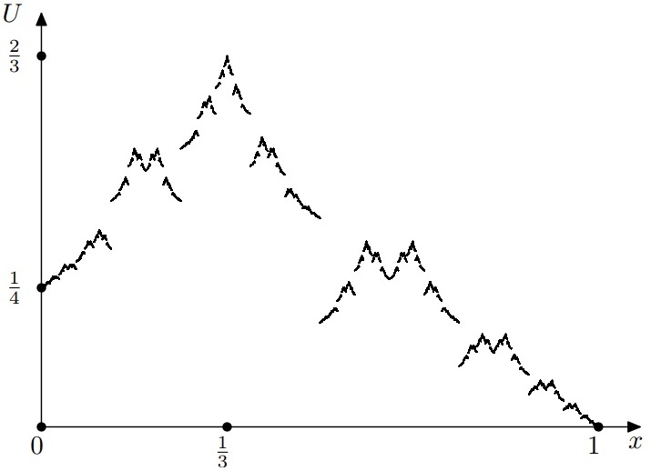
Figure 3: The plot of $U$ for $\lambda=1/2$.

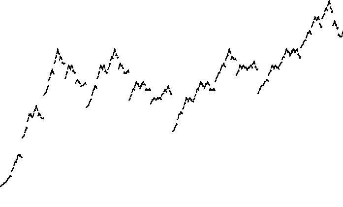
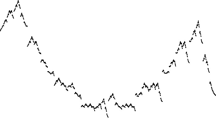
Figure 4: For $\lambda=1/2$, two randomly chosen different segments of the curve $U$ zoomed in $\approx 2^{70}$ times.

Let us provide few formulas followed from Theorem 1.1 and Corollary 1.2. This also reduces some disambiguation in reading (7), (8) and (15), (16) for small $N$ ($N=0$). We have

$$\int_{-1}^{1}V(x)dx=\frac{2}{\sqrt{1-\lambda^{2}}},\ \ \ \int_{-1}^{1}V(x)^{2}dx=\frac{4}{\sqrt{1-\lambda^{4}}\sqrt{1-\lambda^{2}}}-\frac{2}{\sqrt{1-\lambda^{4}}},$$

$$\int_{-1}^{1}V(x)x^{2}dx=\frac{4\sqrt{1-\lambda^{2}}}{3}+\frac{2}{3\sqrt{1-\lambda^{2}}}-4\sqrt{1-\frac{\lambda^{2}}{4}}+\frac{8\sqrt{1-\frac{\lambda^{2}}{16}}}{3},$$

$$\int_{-1}^{1}U(x)dx=\frac{2}{(1-\lambda)\sqrt{1-\lambda^{2}}}-\frac{2}{1-\lambda},$$

$$\int_{-1}^{1}U(x)x^{2}=\frac{\frac{4\sqrt{1-\lambda^{2}}}{3}-4\sqrt{1-\frac{\lambda^{2}}{4}}+\frac{8\sqrt{1-\frac{\lambda^{2}}{16}}}{3}}{1-\frac{\lambda}{4}}+\frac{2}{3(1-\lambda)\sqrt{1-\lambda^{2}}}-\frac{2}{3(1-\lambda)},$$

where the last two integrals are already presented in [1]. Finally, let us conclude with a few words about the comparison of $V(x)$ and $U(x)$. The first function is already a fractal curve, but second one is a “double” fractal curve, since we apply the “fractal” resize-operator ${\mathcal{T}}$ to already fractal curve $V$, see (12) and (13). We can compare the plots of $V$, see Fig. 1, and $U$ presented on Figs. 3 and 4. The first plot I have taken from [1] but the zoomed ones are new.

2 Proof of the main results

2.1 Analytic generating function for $V$.

For $x\in[-1,1]$, let us define the function

$$F(x,z)=1+\lambda z^{x_{0}}+\lambda^{2}z^{x_{0}+x_{1}}+\lambda^{3}z^{x_{0}+x_{1}+x_{2}}+...=1+\sum_{n=0}^{+\infty}\lambda^{n+1}z^{\sum_{j=0}^{n}x_{j}},$$ (23)

where $x_{n}\in\{-1,+1\}$ are given by (1). Since $|\lambda|<1$, it is seen that for any $x\in[-1,1]$ function $F$ is analytic in some open ring containing the circle $|z|=1$. Indeed, each term of the series (23) can be uniformly approximated by the terms of convergent series

$$|F(x,z)|\leqslant 1+\lambda\max\{|z|,|z|^{-1}\}+\lambda^{2}\max\{|z|^{2},|z|^{-2}\}+...\leqslant\frac{1}{1-\lambda|z|}+\frac{1}{1-\lambda|z|^{-1}},$$ (24)

since all $x_{n}\in\{-1,+1\}$. Thus $F(x,z)$ is analytic in $\{z:\ \lambda<|z|<\lambda^{-1}\}$ for any fixed $x\in[-1,1]$. It is seen that $V$ is a free term in the ($z$-)series for $F$, see (2) and (23). Thus, we have

$$V(x)=\mathfrak{f}(F(x,z))=\oint_{|z|=1}F(x,z)\frac{dz}{2\pi iz},$$ (25)

where symbol $\mathfrak{f}$ means the free term in the Laurent series. Using (1) and (23), we derive the functional equation

$$F(\pm\frac{1}{2}+y,z)=1+\lambda z^{\pm 1}F(2y,z),\ \ \ y\in[-\frac{1}{2},\frac{1}{2}],$$ (26)

basic in our research.

2.2 Integrals $\int V(x)^{N}dx$.

For $\alpha\subset\{1,...,N\}$, let us denote

$$F_{\alpha}:=\prod_{j\in\alpha}F(x,z_{j}),\ \ \ z_{\alpha}:=\prod_{j\in\alpha}z_{j},\ \ \ F_{\emptyset}=z_{\emptyset}=1.$$ (27)

Using (26), we obtain

$${\mathcal{J}}F_{\alpha}=\frac{1}{2}{\mathcal{J}}\prod_{j\in\alpha}(1+\lambda z_{j}F_{j})+\frac{1}{2}{\mathcal{J}}\prod_{j\in\alpha}(1+\lambda z_{j}^{-1}F_{j})=\sum_{\beta\subset\alpha}\lambda^{|\beta|}\frac{z_{\beta}+z_{\beta}^{-1}}{2}{\mathcal{J}}F_{\beta}$$ (28)

and, hence,

$${\mathcal{J}}F_{\alpha}=\frac{1}{1-\lambda^{|\alpha|}\frac{z_{\alpha}+z_{\alpha}^{-1}}{2}}\sum_{\beta\subsetneqq\alpha}\lambda^{|\beta|}\frac{z_{\beta}+z_{\beta}^{-1}}{2}{\mathcal{J}}F_{\beta},$$ (29)

where here and below ${\mathcal{J}}\cdot:=\int_{-1}^{1}\cdot dx$ and $|\cdot|$ denotes the number of elements. Thus, we deduce that

$${\mathcal{J}}F_{\alpha}=\frac{1}{1-\lambda^{|\alpha|}\frac{z_{\alpha}+z_{\alpha}^{-1}}{2}}\biggl{(}{\mathcal{J}}1+\sum_{\emptyset\subsetneqq\gamma\subsetneqq...\subsetneqq\beta\subsetneqq\alpha}\lambda^{|\beta|}\frac{\frac{z_{\beta}+z_{\beta}^{-1}}{2}}{1-\lambda^{|\beta|}\frac{z_{\beta}+z_{\beta}^{-1}}{2}}...\lambda^{|\gamma|}\frac{\frac{z_{\gamma}+z_{\gamma}^{-1}}{2}}{1-\lambda^{|\gamma|}\frac{z_{\gamma}+z_{\gamma}^{-1}}{2}}{\mathcal{J}}1\biggr{)},$$ (30)

where the sum is taken over all nested sequences of sets $\emptyset\subsetneqq\gamma\subsetneqq...\subsetneqq\beta\subsetneqq\alpha$, and ${\mathcal{J}}1=2$. Since the sets are embedded strictly in each other, we conclude that the free term of Laurent ($z_{1},...,z_{N}$-)series (30) satisfies the equality

$$\mathfrak{f}({\mathcal{J}}F_{\alpha})=\mathfrak{f}\biggl{(}\frac{1}{1-\lambda^{|\alpha|}\frac{z_{\alpha}+z_{\alpha}^{-1}}{2}}\biggr{)}\mathfrak{f}\biggl{(}2+2\sum_{\emptyset\subsetneqq\gamma\subsetneqq...\subsetneqq\beta\subsetneqq\alpha}\lambda^{|\beta|}\frac{\frac{z_{\beta}+z_{\beta}^{-1}}{2}}{1-\lambda^{|\beta|}\frac{z_{\beta}+z_{\beta}^{-1}}{2}}...\lambda^{|\gamma|}\frac{\frac{z_{\gamma}+z_{\gamma}^{-1}}{2}}{1-\lambda^{|\gamma|}\frac{z_{\gamma}+z_{\gamma}^{-1}}{2}}\biggr{)}$$ (31)

and, similarly,

$$\mathfrak{f}\biggl{(}\lambda^{|\alpha|}{\frac{z_{\alpha}+z_{\alpha}^{-1}}{2}}{\mathcal{J}}F_{\alpha}\biggr{)}=\mathfrak{f}\biggl{(}\frac{\lambda^{|\alpha|}{\frac{z_{\alpha}+z_{\alpha}^{-1}}{2}}}{1-\lambda^{|\alpha|}\frac{z_{\alpha}+z_{\alpha}^{-1}}{2}}\biggr{)}\cdot\\ \mathfrak{f}\biggl{(}2+2\sum_{\emptyset\subsetneqq\gamma\subsetneqq...\subsetneqq\beta\subsetneqq\alpha}\lambda^{|\beta|}\frac{\frac{z_{\beta}+z_{\beta}^{-1}}{2}}{1-\lambda^{|\beta|}\frac{z_{\beta}+z_{\beta}^{-1}}{2}}...\lambda^{|\gamma|}\frac{\frac{z_{\gamma}+z_{\gamma}^{-1}}{2}}{1-\lambda^{|\gamma|}\frac{z_{\gamma}+z_{\gamma}^{-1}}{2}}\biggr{)}.$$ (32)

Using the facts that

$$\mathfrak{f}\biggl{(}\frac{1}{1-\lambda^{|\alpha|}\frac{z_{\alpha}+z_{\alpha}^{-1}}{2}}\biggr{)}=\mathfrak{f}\biggl{(}\frac{1}{1-\lambda^{|\alpha|}\frac{z+z^{-1}}{2}}\biggr{)}=\oint_{|z|=1}\frac{1}{1-\lambda^{|\alpha|}\frac{z+z^{-1}}{2}}\frac{dz}{2\pi iz}=\\ {\rm Res}\biggl{(}\frac{2}{2z-\lambda^{|\alpha|}z^{2}-\lambda^{|\alpha|}};z=\frac{1-\sqrt{1-\lambda^{2|\alpha|}}}{\lambda^{|\alpha|}}\biggr{)}=\frac{1}{\sqrt{1-\lambda^{2|\alpha|}}}$$ (33)

and

$$\mathfrak{f}\biggl{(}\frac{\lambda^{|\alpha|}{\frac{z_{\alpha}+z_{\alpha}^{-1}}{2}}}{1-\lambda^{|\alpha|}\frac{z_{\alpha}+z_{\alpha}^{-1}}{2}}\biggr{)}=\mathfrak{f}\biggl{(}-1+\frac{1}{1-\lambda^{|\alpha|}\frac{z_{\alpha}+z_{\alpha}^{-1}}{2}}\biggr{)}=\frac{1}{\sqrt{1-\lambda^{2|\alpha|}}}-1$$ (34)

along with (31) and(32), we deduce that

$$\mathfrak{f}\biggl{(}\lambda^{|\alpha|}{\frac{z_{\alpha}+z_{\alpha}^{-1}}{2}}{\mathcal{J}}F_{\alpha}\biggr{)}=(1-\sqrt{1-\lambda^{2|\alpha|}})\mathfrak{f}({\mathcal{J}}F_{\alpha}).$$ (35)

Thus, using (35), (29), and simple fact that $\mathfrak{f}({\mathcal{J}}F_{\alpha})=\mathfrak{f}({\mathcal{J}}F_{\alpha^{\prime}})$ if $|\alpha|=|\alpha^{\prime}|$, we obtain

$$\mathfrak{f}({\mathcal{J}}F_{\{1,...,N\}})=\frac{1}{\sqrt{1-\lambda^{2N}}}\biggl{(}2+\sum_{n=1}^{N-1}\binom{N}{n}(1-\sqrt{1-\lambda^{2n}})\mathfrak{f}({\mathcal{J}}F_{\{1,...,n\}})\biggr{)}$$ (36)

that can be written in the matrix form

$$\begin{pmatrix}1&0&0&...&0\\ -1&\sqrt{1-\lambda^{2}}&0&...&0\\ -1&\binom{2}{1}(\sqrt{1-\lambda^{2}}-1)&\sqrt{1-\lambda^{4}}&...&0\\ ...&...&...&...&...\\ -1&\binom{N}{1}(\sqrt{1-\lambda^{2}}-1)&\binom{N}{2}(\sqrt{1-\lambda^{4}}-1)&...&\sqrt{1-\lambda^{2N}}\end{pmatrix}\begin{pmatrix}\mathfrak{f}({\mathcal{J}}F_{\emptyset})\\ \mathfrak{f}({\mathcal{J}}F_{\{1\}})\\ \mathfrak{f}({\mathcal{J}}F_{\{1,2\}})\\ ...\\ \mathfrak{f}({\mathcal{J}}F_{\{1,...,N\}})\end{pmatrix}=\begin{pmatrix}2\\ 0\\ 0\\ ...\\ 0\end{pmatrix}$$

or

$$\begin{pmatrix}1&0&0&...&0\\ 1&-\sqrt{1-\lambda^{2}}&0&...&0\\ 1&\frac{\binom{2}{1}\lambda^{2}}{1+\sqrt{1-\lambda^{2}}}&-\sqrt{1-\lambda^{4}}&...&0\\ ...&...&...&...&...\\ 1&\frac{\binom{N}{1}\lambda^{2}}{1+\sqrt{1-\lambda^{2}}}&\frac{\binom{N}{2}\lambda^{2}}{1+\sqrt{1-\lambda^{2}}}&...&-\sqrt{1-\lambda^{2N}}\end{pmatrix}\begin{pmatrix}\mathfrak{f}({\mathcal{J}}F_{\emptyset})\\ \mathfrak{f}({\mathcal{J}}F_{\{1\}})\\ \mathfrak{f}({\mathcal{J}}F_{\{1,2\}})\\ ...\\ \mathfrak{f}({\mathcal{J}}F_{\{1,...,N\}})\end{pmatrix}=\begin{pmatrix}2\\ 0\\ 0\\ ...\\ 0\end{pmatrix}.$$ (37)

Applying the general Cramer’s rule to the linear system (37) we get the identity

$$p_{0}\mathfrak{f}({\mathcal{J}}F_{\emptyset})+...+p_{N}\mathfrak{f}({\mathcal{J}}F_{\{1,...,N\}})=\\ \frac{-(-1)^{N}}{\prod_{n=1}^{N}\sqrt{1-\lambda^{2n}}}\begin{vmatrix}1&0&0&...&0&2\\ 1&-\sqrt{1-\lambda^{2}}&0&...&0&0\\ 1&\frac{\binom{2}{1}\lambda^{2}}{1+\sqrt{1-\lambda^{2}}}&-\sqrt{1-\lambda^{4}}&...&0&0\\ ...&...&...&...&...\\ 1&\frac{\binom{N}{1}\lambda^{2}}{1+\sqrt{1-\lambda^{2}}}&\frac{\binom{N}{2}\lambda^{4}}{1+\sqrt{1-\lambda^{4}}}&...&-\sqrt{1-\lambda^{2N}}&0\\ p_{0}&p_{1}&p_{2}&...&p_{N}&0\end{vmatrix},\ \ \ p_{i}\in{\mathbb{C}}.$$ (38)

Finally, expanding (38) by the last column and using the obvious extension of (25) based on (27), namely,

$$\int_{-1}^{1}V(x)^{N}dx=\oint_{|z_{1}|=1}...\oint_{|z_{N}|=1}\int_{-1}^{1}F_{\{1,...,N\}}dx\frac{dz_{N}}{2\pi iz_{N}}...\frac{dz_{1}}{2\pi iz_{1}}=\mathfrak{f}({\mathcal{J}}F_{\{1,...,N\}}),$$ (39)

we obtain the announced formula (3). Formula (4) is a simple consequence of (3). The alternative recurrent formula (5) follows from (36) and (39).

2.3 Operator’s identity for $\int V(x)h(x)dx$, $h\in L^{2}$.

We use the notation ${\mathcal{J}}:=\int_{-1}^{1}\cdot dx$ from the previous subsection. Using (26) by analogy with (28), we obtain

$${\mathcal{J}}F\widetilde{h}={\mathcal{J}}\widetilde{h}+\lambda{\mathcal{J}}F\frac{z^{-1}{\mathcal{R}}_{-}+z{\mathcal{R}}_{+}}{2}\widetilde{h},\ \ \forall\widetilde{h}\in L^{2}(-1,1),$$ (40)

that leads to

$${\mathcal{J}}F\biggl{(}1-\lambda\frac{z^{-1}{\mathcal{R}}_{-}+z{\mathcal{R}}_{+}}{2}\biggr{)}\widetilde{h}={\mathcal{J}}\widetilde{h}$$ (41)

or

$${\mathcal{J}}Fh={\mathcal{J}}\biggl{(}1-\lambda\frac{z^{-1}{\mathcal{R}}_{-}+z{\mathcal{R}}_{+}}{2}\biggr{)}^{-1}h,\ \ \forall h\in L^{2}(-1,1)$$ (42)

if the corresponding inverse operator in (42) exists. To show the existence of the inverse operator in (42), it is enough to show that the operator norm $\|z^{-1}{\mathcal{R}}_{-}+z{\mathcal{R}}_{+}\|_{L^{2}\to L^{2}}\leqslant 2$, because using $|\lambda|<1$ we may write the converging geometric series for the inverse operator. The mentioned norm’s inequality follows from

$$\|zf(\frac{x+1}{2})+z^{-1}f(\frac{x-1}{2})\|_{L^{2}(-1,1)}^{2}\leqslant\|zf(\frac{x+1}{2})+z^{-1}f(\frac{x-1}{2})\|_{L^{2}(-1,1)}^{2}+\\ \|zf(\frac{x+1}{2})-z^{-1}f(\frac{x-1}{2})\|_{L^{2}(-1,1)}^{2}=2\|f(\frac{x+1}{2})\|_{L^{2}(-1,1)}^{2}+2\|f(\frac{x-1}{2})\|_{L^{2}(-1,1)}^{2}=\\ 4\|f(x)\|^{2}_{L^{2}(0,1)}+4\|f(x)\|^{2}_{L^{2}(-1,0)}=4\|f(x)\|^{2}_{L^{2}(-1,1)},$$ (43)

where we use the fact that $|z|=1$. Also, it is much easy to check that the operator norm $\|z^{-1}{\mathcal{R}}_{-}+z{\mathcal{R}}_{+}\|_{L^{\infty}\to L^{\infty}}\leqslant 2$ if we consider the space of bounded functions $L^{\infty}$ (or $C$) instead of $L^{2}$. Now, the announced formula (6) follows from (42) and

$$\int_{-1}^{1}V(x)h(x)dx=\oint_{|z|=1}{\mathcal{J}}Fh\frac{dz}{2\pi iz},$$ (44)

that is similar to (25) and (39).

2.4 Integrals $\int V(x)x^{N}dx$.

At first, let us compute

$$\biggl{(}1-\lambda\frac{z^{-1}{\mathcal{R}}_{-}+z{\mathcal{R}}_{+}}{2}\biggr{)}x^{n}=x^{n}-\frac{\lambda z}{2}\biggl{(}\frac{x+1}{2}\biggr{)}^{n}-\frac{\lambda z^{-1}}{2}\biggl{(}\frac{x-1}{2}\biggr{)}^{n}=\\ (1-\frac{\lambda(z+z^{-1})}{2^{n+1}})x^{n}-\frac{\lambda}{2^{n+1}}\sum_{j=0}^{n-1}\binom{n}{j}((-1)^{n-j}z^{-1}+z)x^{j},$$ (45)

that can be written in the matrix form

$$\biggl{(}1-\lambda\frac{z^{-1}{\mathcal{R}}_{-}+z{\mathcal{R}}_{+}}{2}\biggr{)}\begin{pmatrix}1\\ x\\ x^{2}\\ ...\\ x^{N}\end{pmatrix}=\\ \begin{pmatrix}1-\frac{\lambda(z+z^{-1})}{2}&0&0&...&0\\ \frac{-\lambda\binom{1}{0}((-1)^{1-0}z^{-1}+z)}{2^{2}}&1-\frac{\lambda(z+z^{-1})}{2^{2}}&0&...&0\\ \frac{-\lambda\binom{2}{0}((-1)^{2-0}z^{-1}+z)}{2^{3}}&\frac{-\lambda\binom{2}{1}((-1)^{2-1}z^{-1}+z)}{2^{3}}&1-\frac{\lambda(z+z^{-1})}{2^{3}}&...&0\\ ...&...&...&...&...\\ \frac{-\lambda\binom{N}{0}((-1)^{N-0}z^{-1}+z)}{2^{N+1}}&\frac{-\lambda\binom{N}{1}((-1)^{N-1}z^{-1}+z)}{2^{N+1}}&\frac{-\lambda\binom{N}{2}((-1)^{N-2}z^{-1}+z)}{2^{N+1}}&...&1-\frac{\lambda(z+z^{-1})}{2^{N+1}}\end{pmatrix}\begin{pmatrix}1\\ x\\ x^{2}\\ ...\\ x^{N}\end{pmatrix}.$$ (46)

Thus, using the Cramer’s rule, we write

$$\biggl{(}1-\lambda\frac{z^{-1}{\mathcal{R}}_{-}+z{\mathcal{R}}_{+}}{2}\biggr{)}^{-1}\sum_{n=0}^{N}p_{n}x^{n}=\begin{pmatrix}p_{0}&p_{1}&p_{2}&...&p_{N}\end{pmatrix}\biggl{(}1-\lambda\frac{z^{-1}{\mathcal{R}}_{-}+z{\mathcal{R}}_{+}}{2}\biggr{)}^{-1}\begin{pmatrix}1\\ x\\ x^{2}\\ ...\\ x^{N}\end{pmatrix}=\\ \frac{-1}{\prod_{n=1}^{N+1}(1-\frac{\lambda(z+z^{-1})}{2^{n}})}\cdot\\ \begin{vmatrix}1-\frac{\lambda(z+z^{-1})}{2}&0&0&...&0&1\\ \frac{-\lambda\binom{1}{0}((-1)^{1-0}z^{-1}+z)}{2^{2}}&1-\frac{\lambda(z+z^{-1})}{2^{2}}&0&...&0&x\\ \frac{-\lambda\binom{2}{0}((-1)^{2-0}z^{-1}+z)}{2^{3}}&\frac{-\lambda\binom{2}{1}((-1)^{2-1}z^{-1}+z)}{2^{3}}&1-\frac{\lambda(z+z^{-1})}{2^{3}}&...&0&x^{2}\\ ...&...&...&...&...&...\\ \frac{-\lambda\binom{N}{0}((-1)^{N-0}z^{-1}+z)}{2^{N+1}}&\frac{-\lambda\binom{N}{1}((-1)^{N-1}z^{-1}+z)}{2^{N+1}}&\frac{-\lambda\binom{N}{2}((-1)^{N-2}z^{-1}+z)}{2^{N+1}}&...&1-\frac{\lambda(z+z^{-1})}{2^{N+1}}&x^{N}\\ p_{0}&p_{1}&p_{2}&...&p_{N}&0\end{vmatrix}=\\ \frac{-2}{\prod_{n=1}^{N+1}(\lambda z^{2}-2^{n}z+\lambda)}\cdot\\ \begin{vmatrix}\lambda z^{2}-2z+\lambda&0&0&...&0&1\\ \lambda\binom{1}{0}((-1)^{1-0}+z^{2})&\lambda z^{2}-2^{2}z+\lambda&0&...&0&2x\\ \lambda\binom{2}{0}((-1)^{2-0}+z^{2})&\lambda\binom{2}{1}((-1)^{2-1}+z^{2})&\lambda z^{2}-2^{3}z+\lambda&...&0&(2x)^{2}\\ ...&...&...&...&...&...\\ \lambda\binom{N}{0}((-1)^{N-0}+z^{2})&\lambda\binom{N}{1}((-1)^{N-1}+z^{2})&\lambda\binom{N}{2}((-1)^{N-2}+z^{2})&...&\lambda z^{2}-2^{N+1}z+\lambda&(2x)^{N}\\ -zp_{0}&-zp_{1}&-zp_{2}&...&-zp_{N}&0\end{vmatrix}.$$ (47)

Using (47), we write

$${\mathcal{J}}\frac{1}{z}\biggl{(}1-\lambda\frac{z^{-1}{\mathcal{R}}_{-}+z{\mathcal{R}}_{+}}{2}\biggr{)}^{-1}\sum_{n=0}^{N}p_{n}x^{n}=\frac{-2}{\prod_{n=1}^{N+1}(\lambda z^{2}-2^{n}z+\lambda)}\cdot\\ {\footnotesize\begin{vmatrix}\lambda z^{2}-2z+\lambda&0&0&...&0&2\\ \lambda\binom{1}{0}(z^{2}-1)&\lambda z^{2}-2^{2}z+\lambda&0&...&0&0\\ \lambda\binom{2}{0}(z^{2}+1)&\lambda\binom{2}{1}(z^{2}-1)&\lambda z^{2}-2^{3}z+\lambda&...&0&\frac{2^{3}}{3}\\ ...&...&...&...&...&...\\ \lambda\binom{N}{0}((-1)^{N-0}+z^{2})&\lambda\binom{N}{1}((-1)^{N-1}+z^{2})&\lambda\binom{N}{2}((-1)^{N-2}+z^{2})&...&\lambda z^{2}-2^{N+1}z+\lambda&\frac{2^{N}(1+(-1)^{N})}{N+1}\\ -p_{0}&-p_{1}&-p_{2}&...&-p_{N}&0\end{vmatrix}}.$$ (48)

Now, we need to compute the integral of (48) over the unit circle. All poles of RHS in (48) that lies inside the unit ball are simple, they are smaller of the roots of polynomials $2^{n}z-\lambda z^{2}-\lambda$ and have the form

$$z_{n}=\frac{2^{n-1}-\sqrt{4^{n-1}-\lambda^{2}}}{\lambda},\ \ \ n=1,...,N+1.$$ (49)

We assume that $N$ is even. Applying the Cauchy residue theorem to (48) and using identities

$$\lambda(z_{n}^{2}+1)=2^{n}z_{n},\ \ \ \lambda(z_{n}^{2}-1)=-2\sqrt{4^{n-1}-\lambda^{2}}z_{n},$$ (50)

we deduce that

$${\mathcal{J}}\oint_{|z|=1}\biggl{(}1-\lambda\frac{z^{-1}{\mathcal{R}}_{-}+z{\mathcal{R}}_{+}}{2}\biggr{)}^{-1}\sum_{n=0}^{N}p_{n}x^{n}\frac{dz}{2\pi iz}=\sum_{j=1}^{N+1}\frac{1}{\sqrt{4^{j-1}-\lambda^{2}}\prod_{1\leqslant n\neq j\leqslant N+1}z_{j}(2^{j}-2^{n})}\cdot\\ \begin{vmatrix}z_{j}(2^{j}-2)&0&0&...&0&2\\ -2z_{j}\binom{1}{0}\sqrt{4^{j-1}-\lambda^{2}}&z_{j}(2^{j}-2^{2})&0&...&0&0\\ 2^{j}z_{j}\binom{2}{0}&-2z_{j}\binom{2}{1}\sqrt{4^{j-1}-\lambda^{2}}&z_{j}(2^{j}-2^{3})&...&0&\frac{2^{3}}{3}\\ ...&...&...&...&...&...\\ 2^{j}z_{j}\binom{N}{0}&-2z_{j}\binom{N}{1}\sqrt{4^{j-1}-\lambda^{2}}&2^{j}z_{j}\binom{N}{2}&...&z_{j}(2^{j}-2^{N+1})&\frac{2^{N+1}}{N+1}\\ -p_{0}&-p_{1}&-p_{2}&...&-p_{N}&0\end{vmatrix}=\\ \sum_{j=1}^{N+1}\frac{1}{\sqrt{4^{j-1}-\lambda^{2}}\prod_{1\leqslant n\neq j\leqslant N+1}(1-2^{n-j})}\cdot\\ \begin{vmatrix}1-2^{1-j}&0&0&...&0&2\\ -\binom{1}{0}\sqrt{1-\frac{\lambda^{2}}{4^{j-1}}}&1-2^{2-j}&0&...&0&0\\ \binom{2}{0}&-\binom{2}{1}\sqrt{1-\frac{\lambda^{2}}{4^{j-1}}}&1-2^{3-j}&...&0&\frac{2^{3}}{3}\\ ...&...&...&...&...&...\\ \binom{N}{0}&-\binom{N}{1}\sqrt{1-\frac{\lambda^{2}}{4^{j-1}}}&\binom{N}{2}&...&1-2^{N+1-j}&\frac{2^{N+1}}{N+1}\\ -p_{0}&-p_{1}&-p_{2}&...&-p_{N}&0\end{vmatrix},$$ (51)

which with (6) give (7). Formula (8) follows from (7) directly.

2.5 Fourier transform of $V$.

Again, we apply (6). Using the fact that $|\lambda|<1$, and $\|z^{-1}{\mathcal{R}}_{-}+z{\mathcal{R}}_{+}\|\leqslant 2$ for $|z|=1$, we obtain the following geometric series expansion

$$\biggl{(}1-\lambda\frac{e^{-i\varphi}{\mathcal{R}}_{-}+e^{i\varphi}{\mathcal{R}}_{+}}{2}\biggr{)}^{-1}e^{i\omega x}=\sum_{n=0}^{\infty}\lambda^{n}\biggl{(}\frac{e^{-i\varphi}{\mathcal{R}}_{-}+e^{i\varphi}{\mathcal{R}}_{+}}{2}\biggr{)}^{n}e^{i\omega x}=\\ \sum_{n=0}^{\infty}\lambda^{n}\biggl{(}\frac{e^{-i\varphi-i\frac{\omega}{2}}+e^{i\varphi+i\frac{\omega}{2}}}{2}\biggr{)}...\biggl{(}\frac{e^{-i\varphi-i\frac{\omega}{2^{n}}}+e^{i\varphi+i\frac{\omega}{2^{n}}}}{2}\biggr{)}e^{i\frac{\omega x}{2^{n}}}=\sum_{n=0}^{\infty}e^{i\frac{\omega x}{2^{n}}}\lambda^{n}\prod_{j=1}^{n}\cos(\varphi+\frac{\omega}{2^{j}}),$$ (52)

where $\varphi\in{\mathbb{R}}$ and $\omega\in{\mathbb{C}}$. Thus, (52) along with (6) give us

$$\int_{-1}^{1}e^{i\omega x}V(x)dx={\mathcal{J}}\int_{-\pi}^{\pi}\biggl{(}1-\lambda\frac{e^{-i\varphi}{\mathcal{R}}_{-}+e^{i\varphi}{\mathcal{R}}_{+}}{2}\biggr{)}^{-1}e^{i\omega x}\frac{d\varphi}{2\pi}=\frac{1}{\pi}\int_{-\pi}^{\pi}C(\varphi,\omega),$$ (53)

where

$$C(\varphi,\omega)=\sum_{n=0}^{\infty}\lambda^{n}\frac{2^{n}}{\omega}\sin\frac{\omega}{2^{n}}\prod_{j=1}^{n}\cos(\varphi+\frac{\omega}{2^{j}})=\\ \frac{\sin\omega}{\omega}\sum_{n=0}^{\infty}\prod_{j=1}^{n}\frac{\lambda\cos(\varphi+\frac{\omega}{2^{j}})}{\cos\frac{\omega}{2^{j}}}=\frac{\sin\omega}{\omega}\cdot\cfrac{1}{1-\cfrac{\frac{\lambda\cos(\varphi+\frac{\omega}{2})}{\cos\frac{\omega}{2}}}{1+\frac{\lambda\cos(\varphi+\frac{\omega}{2})}{\cos\frac{\omega}{2}}-\cfrac{\frac{\lambda\cos(\varphi+\frac{\omega}{4})}{\cos\frac{\omega}{4}}}{1+\frac{\lambda\cos(\varphi+\frac{\omega}{4})}{\cos\frac{\omega}{4}}-\cfrac{\frac{\lambda\cos(\varphi+\frac{\omega}{8})}{\cos\frac{\omega}{8}}}{1+\frac{\lambda\cos(\varphi+\frac{\omega}{8})}{\cos\frac{\omega}{8}}-...}}}}=\\ \frac{\sin\omega}{\omega}\cdot\cfrac{1}{1-\cfrac{\lambda\cos(\varphi+\frac{\omega}{2})}{\cos\frac{\omega}{2}+\lambda\cos(\varphi+\frac{\omega}{2})-\cfrac{\lambda\cos\frac{\omega}{2}\cos(\varphi+\frac{\omega}{4})}{\cos\frac{\omega}{4}+\lambda\cos(\varphi+\frac{\omega}{4})-\cfrac{\lambda\cos\frac{\omega}{4}\cos(\varphi+\frac{\omega}{8})}{\cos\frac{\omega}{8}+\lambda\cos(\varphi+\frac{\omega}{8})-...}}}}.$$ (54)

To derive last three identities in (54), we have used the identity $\sin\omega=2^{n}\sin\frac{\omega}{2^{n}}\prod_{j=1}^{m}\cos\frac{\omega}{2^{j}}$ and Euler’s continued fraction formula. Note that while the first identity in (54) is valid for $\varphi\in{\mathbb{R}}$, $\omega\in{\mathbb{C}}$ (for $\omega=0$ there is a limit $\frac{\sin\omega}{\omega}\to 1$), the other identities in (54) are formally valid for $\varphi\in{\mathbb{R}}$, $\omega\in{\mathbb{C}}\setminus\pi{\mathbb{Z}}$. Using (53) and (54) and the fact that $V$ is even function, we obtain the announced formulas (9) and (10).

2.6 Proof of Corollary 1.2.iii).

Using the generating function for Bernoulli polynomials, we obtain

$$P(t,x):=\sum_{n=0}^{+\infty}P_{n}(x)\frac{t^{n}}{n!}=\sum_{n=0}^{+\infty}2^{n}B_{n}(\frac{x+1}{2})\frac{t^{n}}{n!}=\frac{2te^{2t\frac{x+1}{2}}}{e^{2t}-1}=\frac{t}{\sinh t}e^{tx},$$ (55)

which with

$$({\mathcal{R}}_{-}+{\mathcal{R}}_{+})P(t,x)=\frac{t}{\sinh t}({\mathcal{R}}_{-}+{\mathcal{R}}_{+})e^{tx}=\frac{t}{\sinh t}(e^{\frac{t}{2}}+e^{-\frac{t}{2}})e^{\frac{tx}{2}}=2P(\frac{t}{2},x)$$ (56)

leads to

$$({\mathcal{R}}_{-}+{\mathcal{R}}_{+})P_{n}(x)=\frac{2}{2^{n}}P_{n}(x).$$ (57)

Using identity ${\mathcal{D}}^{k}e^{tx}=t^{k}e^{tx}$, $k\geqslant 0$ along with (55), we obtain

$$P(t,x)=\frac{{\mathcal{D}}}{\sinh{\mathcal{D}}}e^{tx}.$$ (58)

Expanding $e^{tx}$ into the Taylor series and using (58) along with the definition (55) we obtain

$$P_{n}(x)=\frac{{\mathcal{D}}}{\sinh{\mathcal{D}}}x^{n}$$ (59)

that also leads to

$${\mathcal{D}}P_{n}(x)={\mathcal{D}}\frac{{\mathcal{D}}}{\sinh{\mathcal{D}}}x^{n}=\frac{{\mathcal{D}}}{\sinh{\mathcal{D}}}{\mathcal{D}}x^{n}=n\frac{{\mathcal{D}}}{\sinh{\mathcal{D}}}x^{n-1}=nP_{n-1}(x).$$ (60)

Both identities (59) and (60) for even $n$ give us

$$x^{n}=\frac{\sinh{\mathcal{D}}}{{\mathcal{D}}}P_{n}(x)=\sum_{j=0}^{\frac{n}{2}}\frac{1}{(2j+1)!}{\mathcal{D}}^{2j}P_{n}(x)=\sum_{j=0}^{\frac{n}{2}}\frac{\binom{n}{2j}}{2j+1}P_{n-2j}(x).$$ (61)

Now, all the ingredients are ready. Formula (17) follows from (14) and (57). Formula (18) follows from (17) and (61). Formulas (55), (59) and (60) imply (19).

References

- [1] A. A. Kutsenko. On some explicit integrals related to “fractal mountains”. https://arxiv.org/abs/2108.04237