Sorting with Teams

Abstract

We fully solve a sorting problem with heterogeneous firms and multiple heterogeneous workers whose skills are imperfect substitutes. We show that optimal sorting, which we call mixed and countermonotonic, is comprised of two regions. In the first region, mediocre firms sort with mediocre workers and coworkers such that the output losses are equal across all these teams (mixing). In the second region, a high skill worker sorts with low skill coworkers and a high productivity firm (countermonotonicity). We characterize the equilibrium wages and firm values. Quantitatively, our model can generate the dispersion of earnings within and across US firms.

JEL-Codes: J01, D31, C78.
Keywords: Sorting, Teams, Assignment.

1 Introduction

How do heterogeneous workers sort to work in teams at heterogeneous firms? Which workers work together, and what firm do they work for? How do worker earnings depend on their employer, their coworkers, as well as other firms and workers in the economy? How does the firm value vary with the workers they hire? To answer these questions, we study the sorting of multiple heterogeneous workers into teams at heterogeneous firms when workers’ skills are imperfect substitutes.

The traditional approach to one worker, one firm assignment problems is to provide conditions under which sorting is assortative. Becker (1973) shows that optimal sorting is positive under supermodular technologies and negative under submodular technologies. Positive sorting, or comonotonicity, readily extends to settings with multiple workers and is generally optimal with supermodular technologies. On the other hand, negative sorting, or countermonotonicity, does not have a simple multi-type equivalent.

An important open question is how to characterize sorting of heterogeneous firms with multiple heterogeneous workers when technology is submodular. We show that this problem can be analyzed as a multimarginal optimal transport problem and fully characterize the solution.

We are the first to fully solve a sorting problem with firm heterogeneity and multiple heterogeneous workers whose skills are imperfect substitutes, that is, when the technology is submodular. In doing so, this paper makes two contributions. First, we show that an equilibrium assignment is characterized by two types of assignment regions. In the first region, mediocre firms sort with mediocre workers and coworkers so that output losses are equal across all these teams (mixed assignment). In the second region, high skill workers sort with low skill coworkers and a high productivity firm, while high productivity firms employ low skill workers and a single high skill coworker (countermonotonic assignment). We call this a mixed and countermonotonic assignment. Second, we fully characterize the equilibrium assignment as well as workers’ wages and firm values. We illustrate our theory with a quantitative application to earnings dispersion within and across U.S. firms.

We develop our findings using a transferable utility assignment model with worker peer effects and firm heterogeneity. In order to illustrate our theory, consider a simple production and team technology. The output of a firm is the product of the value of their project, or productivity $z$, and the probability their worker team is able to solve production problems $q$. When workers independently do not know how to solve a problem with probability $x_{i}$, team quality with workers $(x_{1},x_{2},\dots,x_{m})$ is $q=1-\prod\limits_{i=1}^{m}x_{i}$, and output is $y(x_{1},x_{2},\dots,x_{m},z)=zq=\big{(}1-\prod\limits_{i=1}^{m}x_{i}\big{)}z$. Production is supermodular in team quality and productivity, and submodular in worker skills and productivity. Workers are imperfect substitutes, with peer effects in output scaling with the project value.

We show there are two regions to an optimal assignment. The first region is the mixed set. Mixing means that the output loss, $z\prod x_{i}$, is identical for all teams. We start with the observation that mixing is optimal whenever it is feasible. Equalizing output loss $z\prod x_{i}$ across teams is optimal as average expected losses attain their lower bound if and only if output losses are equal across all teams following Jensen’s inequality. Mixing implies that firms with identical projects may hire different teams of workers which have the same overall quality.

Mixing, however, does not fully describe equilibrium assignment as it is not feasible everywhere. We show that optimal sorting features the maximal mixed set combined with countermonotonic regions. To develop intuition for the optimality of countermonotonic sets, we note that at the boundary of the mixed set, the lowest value project is sorted with identical low-skill workers (high $x_{i}$). Similarly, a project which has zero value employs workers who do not know how to solve a problem ($x_{i}=1$). Applying this reasoning to other low value projects outside the mixed set, these projects are countermonotonically sorted with low-skill workers.

In order to establish equilibrium properties of worker wages and firm values we characterize the dual problem. We show that the derivative of the wage schedule is equal to the marginal worker product, or $-z\prod\limits_{j\neq i}x_{j}$. The increase in output obtained by replacing a worker with a slightly more skilled worker, keeping their coworkers and their firm unchanged, has to equal the increase in wages necessary to hire the higher-skill worker. More skilled workers work with coworkers and a firm that has greater expected output losses, implying a convex wage schedule.

Our main result is derived in a setting with heterogeneous distributions of workers and firms and teams of $n\geq 2$ members. We prove that a mixed and countermonotonic assignment is optimal, derive its dual, and thus characterize an equilibrium. We establish the optimality of a mixed and countermonotonic assignment by using a majorization inequality (Hardy, Littlewood, and Pólya, 1929; Karamata, 1932; Pečarić, 1984). We combine our characterization of optimal assignments with a duality argument for multimarginal optimal transport problems (Kellerer, 1984) to derive worker wages and firm values. Finally, we discuss how our results apply to more general production structures.

Having characterized equilibrium, we quantitatively illustrate the theory using administrative U.S. earnings records. Since a characteristic feature of our paper among assignment models is that we obtain distinct distributions of earnings within heterogeneous firms, we apply our model to evaluate the dispersion in earnings within and across U.S. firms.

Our model can generate the dispersion of earnings as well as its decomposition between and within firms as empirically documented by Song, Price, Guvenen, Bloom, and Von Wachter (2019). We use the cross-sectional distribution of earnings and the decomposition of earnings variation into within-firm and between-firm variation to estimate the underlying distributions of worker skills and firm values. We show that only changing the distribution of firm projects between 1981 and 2013, the share of within-firm earnings dispersion would have increased by 22 percentage points. Changing the distribution of workers, we show that the share of within-firm earnings dispersion would have decreased by 38 percentage points. That is, our counterfactual analysis shows that both the changes in the worker and project distributions are important in the model in generating the observed change in earnings dispersion.

Related Literature. There is an extensive literature on one-to-one assignment models in the tradition of Becker (1973). This literature, in particular, analyzes conditions under which sorting is positive or negative. Our contribution is to characterize sorting for an assignment problem with heterogeneous firms and multiple heterogeneous workers whose skills are imperfect substitutes. We provide a complete equilibrium characterization for this problem, and show this equilibrium features neither positive nor negative sorting.

The closest to our work is a literature that studies negative sorting with more than two agents. Ahlin (2017), Chade and Eeckhout (2018) and Eeckhout (2018) argue it is neither evident how to define negative sorting in this case, nor how to characterize an optimal assignment when production is submodular, and also derive insightful partial characterizations of the equilibrium. Ahlin (2017) also develops a quantitative application to group formation in villages. In our paper, we fully characterize optimal sorting for dimensions greater than two with a submodular technology.

An alternative approach to multiworker firms in assignment models is due to Eeckhout and Kircher (2018). They develop a model in which firms sort with a single type of worker, and choose how many workers of this type to employ. Eeckhout and Kircher (2018) develop conditions under which sorting is positive or negative. Importantly, they assume the firm technology is additively separable between workers of different types, so the marginal worker product is independent from other types of workers within the firm. This paper differs from Eeckhout and Kircher (2018) by focusing on firms of fixed size and by incorporating peer effects. Workers are instead imperfect substitutes under a submodular technology, and their marginal product does depend on their coworkers.

This paper relates to a growing literature which uses optimal transport theory to solve economic problem, see Galichon (2018) for a comprehensive overview. Specifically, there is an important line of work on multidimensional sorting and multi-market problems, working with optimal transport theory, such as Dupuy and Galichon (2014), McCann, Shi, Siow, and Wolthoff (2015), Lindenlaub (2017), Chiappori, McCann, and Pass (2017), Chiappori, Salanié, and Weiss (2017), Ocampo Díaz (2022), Lindenlaub and Postel-Vinay (2020) and Galichon and Salanié (2021). Our assignment problem instead results in a sorting problem where each dimension of heterogeneity sorts with an endogenous multidimensional distribution.

Another literature, following Garicano and Rossi-Hansberg (2006), solves hierarchical assignment models with heterogeneous workers. Similar to Garicano (2000), workers differ in their knowledge, which governs the probability that they know how to solve a production problem. Knowledge is assumed to be cumulative, so that more skilled workers know how to solve a problem whenever less skilled workers do. A key implication is that production is supermodular in worker skill, so that equilibrium sorting is positive. In line with these papers, our workers differ in the probability that they know how to solve production problems. Knowledge, however, is not cumulative, allowing for the possibility that less skilled workers know how to solve a problem when more skilled workers do not. As a result, our production technology is not supermodular, and hence optimal sorting is not positive.

To characterize our equilibrium, we build on the optimal transport literature in mathematics that develops tools to solve multimarginal transport problems. While this is an active area of recent research with a number of applications, understanding of the problem is far from complete and is fractured (for examples of different settings and costs, see Gangbo and Świech (1998), Carlier and Ekeland (2010), Kim and Pass (2014), and Gladkov and Zimin (2020)). Our paper studies a submodular cost function and introduces firm production, non-uniform distributions of workers and firms, and uses this to understand equilibrium sorting, worker wages, and firm values. In the literature on risk aggregation and insurance, Bernard, Jiang, and Wang (2014), Embrechts, Puccetti, Rüschendorf, Wang, and Beleraj (2014), Puccetti and Wang (2015) and Wang and Wang (2016) study properties of aggregate risk as the sum of individual risks. Similar to them, we study the minimization of output losses (risks) incurred by teams of workers and firms in the economy. Different from them, our interest lie in the distribution of output losses and characterizing sorting patterns of workers that generate maximum aggregate output. Moreover, we characterize the dual problem to characterize the distribution of wages and firm values.

2 Model

We study an economy in which agents with heterogeneous skills choose their firm and coworkers to work with. This is an assignment problem extended to incorporate multiple workers in each firm. Our setup results in a sorting problem between multiple workers with each firm for a submodular production technology.

2.1 Environment

Agents. There are $m\geq 2$ groups of risk-neutral workers and a single group of risk-neutral firms. Each group has mass one.

Workers differ in skills. The skill is indexed by a single number $x_{i}\in X=[0,1]$, which captures the probability that the worker does not know how to solve a problem. For example, a worker with skill $x_{i}=0.1$ knows how to solve a problem with 90 percent probability. High skill workers have low $x_{i}$. The distribution of each group of workers has cumulative distribution function $F_{x}(x_{i})$ and corresponding continuous density function $f_{x}(x_{i})$.

Firms differ in productivity $z\in Z=[0,1]$, capturing the value of their projects. High value firms have a high $z$. The distribution of firms has cumulative distribution function $F_{z}(z)$ and continuous density function $f_{z}(z)$. The cumulative distribution functions are strictly increasing and continuous. The inverse distribution function for firms is so that $I_{z}(p_{z})$ for percentile $p_{z}\in[0,1]$ is the unique number $z$ that satisfies $F_{z}(z)=p_{z}$. Thus, the percentile $p_{z}$ corresponds to the value $z$ in the firm distribution. The inverse distribution function for workers $I_{x}$ is defined analogously.

Technology. A team comprises of $m$ workers that encounter a problem in production. These workers solve a problem when at least one of them knows how to solve it. Since the probability that worker $i$ does not know the solution is $x_{i}$, independent of their coworker knowing the solution, the probability of successful production with workers $(x_{1},x_{2},\dots,x_{m})$ is:

$$q=h(x_{1},x_{2},\dots,x_{m})=1-\prod\limits_{i=1}^{m}x_{i}.$$ (1)

The team quality function $h$ is a symmetric, submodular function in worker types, so workers are substitutes.

A firm of type $z$ that employs a team of quality $q$ produces output according to:

$$g(q,z)=qz.$$ (2)

The production function $g$ is supermodular in team quality $q$ and firm type $z$. Team quality and the project are complements in production. Combining the technology (2) with the team quality function (1), firm output $y$ is:

$$y(x_{1},x_{2},\dots,x_{m},z)=\Big{(}1-\prod\limits_{i=1}^{m}x_{i}\Big{)}z.$$ (3)

Firm output is a submodular function in worker and firm type. The marginal product of worker $x_{i}$ is:

$$m(x_{i})=y_{i}(x_{1},x_{2},\dots,x_{m},z)=-z\prod\limits_{j\neq i}x_{j}\leq 0.$$ (4)

When a worker is less skilled, that is, less likely to know how to solve a problem, output decreases. The marginal product of every worker depends only on the skills of their coworker and the firm they work with.

Assignment. An assignment prescribes for every worker coworkers to work with and a firm to work for. Given a distribution of workers $F_{x}$ and a distribution of firms $F_{z}$, the set of feasible assignment functions is $\Pi:=\Pi(F_{x},\dots,F_{x},F_{z})$ which is the set of probability measures $\pi$ on $X\times\dots\times X\times Z$ such that the marginal distributions of $\pi$ onto $X$ and $Z$ are equal to $F_{x}$ and $F_{z}$ respectively. Feasibility of an assignment function is equivalent to labor market clearing, that is, all workers and firms are sorted.

2.2 Assignment Problem

We solve two problems to characterize an equilibrium.

Primal Problem. We first solve a primal problem to find an optimal sorting:

$$\max_{\pi\in\Pi}\int y(x_{1},x_{2},\dots,x_{m},z)\text{d}\pi.$$ (5)

This problem is to choose an assignment $\pi$ to maximize production. It is equivalent to, in terms of choosing an optimal assignment, minimizing output losses. Output losses are the product of the project value $z$ and the probability of failure by a team of workers which is given by $x_{1}\cdots x_{m}$, that is, a loss $x_{1}\cdots x_{m}z$. We thus equivalently represent the planning problem as:

$$\min_{\pi\in\Pi}\;\int x_{1}\cdots x_{m}z\text{d}\pi,$$ (6)

which is an optimal transport problem in the tradition of Monge (1781) and Kantorovich (1942), with multiple marginal distributions. The number of marginal distributions is given by $n=m+1$, comprising $m$ workers in a team and a project.

Dual Problem. To obtain equilibrium wages $w$ and firm values $v$, we solve a dual problem. The dual problem is to choose functions $w$ and $v$ that solve:

$$\min\;\sum^{m}_{i=1}\int w(x_{i})\text{d}F_{x}+\int v(z)\text{d}F_{z},$$ (7)

subject to the constraint that $\sum w(x_{i})+v(z)\geq y(x_{1},x_{2},\dots,x_{m},z)$ for any $(x_{1},x_{2},\dots,x_{m},z)$.

3 Intuition for the Main Result

This section provides intuition for optimal sorting. We consider the case where all distributions are identical.

The core idea of the optimal sorting is based on three observations. First, Jensen’s inequality bounds aggregate output losses from below:

$$\int x_{1}\cdots x_{m}z\text{d}\pi\geq\exp\Big{(}\int\log x_{1}\cdots x_{m}z\text{d}\pi\Big{)}.$$ (8)

Second, the lower bound is independent of assignment $\pi$ due to feasibility:

$$\exp\Big{(}\int\log x_{1}\cdots x_{m}z\text{d}\pi\Big{)}=\exp\Big{(}\int\log x_{1}\text{d}F+...+\int\log x_{m}\text{d}F+\int\log z\text{d}F\Big{)}.$$ (9)

The right hand side is a constant $\mathcal{C}$ as $\int\log z\text{d}F$ and $\int\log x_{i}\text{d}F$ depend only on the marginal distributions. Combining (8) and (9), the aggregate output loss is bounded below by $\mathcal{C}$:

$$\int x_{1}\cdots x_{m}z\text{d}\pi\geq\mathcal{C}.$$ (10)

Third, by Jensen’s inequality the minimum given by the right-hand side is attained when the output loss is equal across all teams and equal to $\mathcal{C}$. We refer to the set of teams with the same output loss $\mathcal{C}$ as mixed. When an assignment is mixed, it is optimal as it minimizes aggregate losses (6).

While mixing is optimal when it is feasible, it is not feasible everywhere. Consider a project $z=0$ in a mixed assignment. Then the output loss $x_{1}x_{2}\dots x_{m}z$ has to be equal to zero for all teams. Thus, mixed is not feasible everywhere.

We show that the optimal assignment is the largest possible set of mixed teams combined with countermonotonic sets. The intuition for this result is as follows.

Jensen’s inequality suggests that it is optimal to have the largest set of mixed teams. Consider a mixed set with the workers and firms between percentiles $\underline{p}$ and $\bar{p}$ in their distribution, that is, the values $[I(\underline{p}),I(\bar{p})]$ from each distribution. We now show that $\mathcal{C}=I(\underline{p})I^{m}(\bar{p})$ for the largest possible set of mixed teams. The maximal output loss on a low-value project $z=I(\underline{p})$ is attained by pairing this project with the lowest-skill workers $x_{i}=I(\bar{p})$ for all $i$. This team incurs an output loss $I(\underline{p})I^{m}(\bar{p})$ and thus $\mathcal{C}\leq I(\underline{p})I^{m}(\bar{p})$. For the maximal feasible mixed set, this condition has to hold with equality $\mathcal{C}=I(\underline{p})I^{m}(\bar{p})$.

We next describe the reasoning behind the countermonotonic sets. First, note that the lowest value project $z=I(\underline{p})$ in the mixed set is paired with $m$ identical low skill workers $I(\bar{p})$ in this set to attain the loss $\mathcal{C}=I(\underline{p})I^{m}(\bar{p})$. Second, it is naturally optimal to pair the lowest value project $z=0$ with $m$ lowest skill workers $x_{i}=1$, attaining zero loss. Interpolating this logic between the project values $z=0$ and $z=I(\underline{p})$, projects below $I(\underline{p})$ are sorted countermonotonically to $m$ identical low skill workers. This generates a countermonotic set for low value projects $z\in[0,I(\underline{p}))$ with $m$ identical low skill workers $x_{i}\in(I(\bar{p}),1]$. By symmetry, high skill workers $x_{j}\in[0,I(\underline{p}))$ are paired with $m-1$ low skill coworkers $x_{i}\in(I(\bar{p}),1]$ and a high value project $z\in(I(\bar{p}),1]$. Since both low value projects $z$ and high skill workers $x_{j}$ for all $j\neq i$ are assigned to teams with low skill workers $x_{i}$, percentiles $[0,p)$ of firms $z$ and high-skill workers $x_{j}$ absorb measure $mp$ of low-skill coworker $x_{i}$. Percentile $p\in[0,\underline{p})$ of the project distribution is thus sorted with percentile $1-mp$ of the worker distributions. The least valuable project $p=0$ employs the least productive workers at percentile $1$; a project at percentile $\underline{p}$ is sorted with identical workers ranked $1-m\underline{p}=\bar{p}$. This team incurs loss $I^{m}(\bar{p})I(\underline{p})=\mathcal{C}$, identical to the loss for all teams on the mixed set.

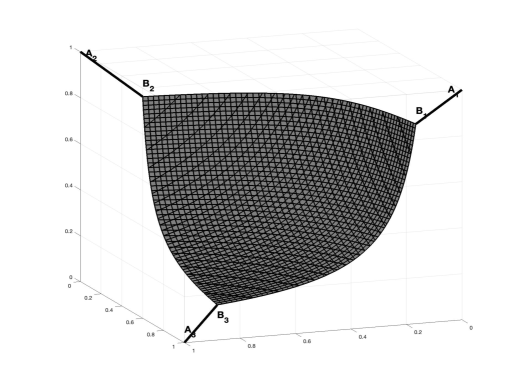
Figure 1: Support of the Assignment

Figure 1 plots an example for the support for an optimal assignment when each team employs two workers, $m=2$. The $x$-axis and $y$-axis show the skill of the worker $x_{1}$ and their coworker ${x_{2}}$, while the $z$-axis plots the value of the firm project $z$.

In sum, we provided intuition for the following solution. Pair high skill workers with low skill workers on valuable projects, until, at some point, mediocre workers can be paired with firms such that output losses are identical for all mediocre teams. Figure 1 visualizes the support of this candidate solution with two workers. The countermonotonic sets corresponding to teams with high skill workers $x_{1}$ and $x_{2}$ is represented by $A_{1}B_{1}$ and $A_{2}B_{2}$, while the countermonotonic set that corresponds to teams with low value projects $z$ is $A_{3}B_{3}$. The mixed set is represented by $B_{1}B_{2}B_{3}$.

4 Main Results

We next show that a mixed and countermonotonic assignment solves the planning problem with heterogeneous continuous marginal distributions and characterize the dual solution for wages and firm values.

4.1 Mixed and Countermonotonic Assignment

We generalize the assignment in Section 3 to heterogeneous marginal distributions by developing three insights from the intuition for the case of homogenous marginal distributions.

First, in the case of homogenous distributions, each distribution is segmented into three parts: low values $[0,I(\underline{p}\vphantom{\bar{p}})]$, medium values $[I(\underline{p}\vphantom{\bar{p}}),I(\bar{p})]$, and high values $[I(\bar{p}),1]$. The measure of medium values is $\bar{p}-\underline{p}=1-q$. With heterogeneous distributions, we segment all distributions into three parts, each indexed by $i\in\{1,\dots,n\}$: low values $[0,I_{i}(\underline{p}\vphantom{\bar{p}}_{i})]$, medium values $[I_{i}(\underline{p}\vphantom{\bar{p}}_{i}),I_{i}(\bar{p}_{i})]$, and high values $[I_{i}(\bar{p}_{i}),1]$. The measure of medium values is $\bar{p}_{i}-\underline{p}\vphantom{\bar{p}}_{i}=1-q$, identical across distributions.

Second, we consider the ranking of output losses across teams. In the homogenous case, the loss is largest for teams in the mixed set which has measure $1-q$. The remaining teams are in countermonotonic sets with measure $q$. For each percentile $t\leq q$, there are $n$ teams located at the $t$-th percentile of the loss distribution, one in each countermonotonic set. Each team consists of a low value $I(\frac{t}{n})$ from one of the distributions and $m$ high values $I(1-\frac{m}{n}t)$ from the remaining distributions. With heterogenous distributions, the loss is as well largest for teams in the mixed set which has measure $1-q$. There are also $n$ teams located at every percentile $t\leq q$. Each team consists of a low value $I_{i}(\underline{t}_{i}(t))$ from one of the distributions and $m$ high values $I_{j}(1-\bar{t}_{j}(t))$ from the remaining distributions $j\neq i$, where the functions $\underline{t}_{i}$ and $\bar{t}_{i}$ are both increasing. The function $\underline{t}_{i}(t)$ gives the percentile of the low value drawn from distribution $i$ at the $t$-th percentile of the team loss distribution. Similarly, the function $\bar{t}_{j}(t)$ yields the percentile of the high value drawn from distribution $j$ at the $t$-th percentile of the team loss distribution. In the homogenous case, $\underline{t}_{i}(t)=\frac{t}{n}$ and $\bar{t}_{j}(t)=\frac{m}{n}t$.

Finally, in the case of homogeneous distributions, mixed teams contain agents in $[I(\underline{p}),I(\bar{p})]$, and their losses are all identical and equal to $I(\underline{p})I(\bar{p})^{m}$. With heterogenous distributions, mixed teams contain values in $[I_{i}(\underline{p}\vphantom{\bar{p}}_{i}),I(\bar{p}_{i})]$ and attain identical losses $\mathcal{C}=\prod x_{i}$, where for all $i$:

$$\mathcal{C}=I_{i}(\underline{p}\vphantom{\bar{p}}_{i})\prod\limits_{j\neq i}I_{j}(\bar{p}_{j}).$$ (11)

We use the generalization of features of the optimal sorting with homogeneous distributions to define a mixed and countermonotonic assignment for the case of heterogeneous distributions.

Definition 1.

A mixed and countermonotonic assignment is a collection of continuous increasing functions $\{(\underline{t}_{i},\bar{t}_{i})\}_{i=1}^{n}$, thresholds $\{(\underline{p}\vphantom{\bar{p}}_{i},\bar{p}_{i})\}_{i=1}^{n}$, and an assignment $\pi\in\Pi(\{F_{i}\}_{i=1}^{n})$ satisfying:

1. The mass of agents in the mixed sets $[I_{i}(\underline{p}\vphantom{\bar{p}}_{i}),I(\bar{p}_{i})]$ is identical for all distributions $1-q=\bar{p}_{i}-\underline{p}\vphantom{\bar{p}}_{i}$ for all $i$.

2. The support of assignment $\pi$ consists of ($1$) a mixed assignment; and ($2$) $n$ countermonotonic sets so that for all $0\leq t\leq q$ the assignment is countermonotonic:
   $b_{i}(t)=(b_{i1}(t),\dots,b_{in}(t))$ with $b_{ii}(t)=I_{i}(\underline{t}_{i}(t))$ and $b_{ij}(t)=I_{j}(1-\bar{t}_{j}(t))$ if $i\neq j$.

3. For each $i$, $b_{i}(t)$ starts at $(1,\dots,1,0,1,\dots,1)$ and ends at $(I_{1}(\bar{p}_{1}),\dots,I_{i}(\underline{p}\vphantom{\bar{p}}_{i}),\dots,I_{n}(\bar{p}_{n}))$. Equivalently, this means that $\underline{t}_{i}(0)=\bar{t}_{i}(0)=0$, $\underline{t}_{i}(q)=\underline{p}_{i}$, and $1-\bar{t}_{i}(q)=\bar{p}_{i}$ for each $i$.

4. For each percentile $t\leq q$, there are $n$ teams located at the $t$-th percentile, when teams are ranked according to their output losses. Team $i$ is located on the countermonotonic set at $b_{i}(t)$. All other teams are mixed and have identically large losses equal to $\mathcal{C}$ given by (11).

4.2 Planning Problem

In this section, we prove our main result that a mixed and countermonotonic assignment, following Definition 1, is optimal.

Theorem 1.

Any mixed and countermonotonic assignment $\pi\in\Pi$ solves the planning problem (5).

We provide a sketch of the proof. Let $\gamma$ be the distribution of logarithmic output losses induced by assignment $\pi$. The associated inverse cumulative distribution function is $I_{\gamma}$. That is, logarithmic losses by a team at percentile $p$ in the loss ranking are given by $I_{\gamma}(p)$ when teams are sorted in increasing loss order. We show that an assignment $\pi^{*}$ is optimal by showing that output losses are greater under any other assignment $\pi$. That is, $\int\ell(x_{1},x_{2},\dots,x_{n},z)\text{d}\pi^{\ast}\leq\int\ell(x_{1},x_{2},\dots,x_{m},z)\text{d}\pi$ or, equivalently, $\int_{0}^{1}\exp(I_{\gamma^{\ast}}(p))\text{d}p\leq\int_{0}^{1}\exp(I_{\gamma}(p))\text{d}p$.

Specifically, we establish optimality by proving that logarithmic output losses under the optimal assignment are smaller in convex order than the logarithmic output losses under any other feasible assignment. The proof is constructed using the integral version of the majorization inequality (Hardy, Littlewood, and Pólya, 1929; Karamata, 1932; Pečarić, 1984).

Majorization Inequality. Let $h$ be a continuous convex function, and let $s_{1}$ and $s_{2}$ be non-decreasing functions on the unit interval. Suppose

$$1.\int_{0}^{1}s_{1}(p)\text{d}p =\int_{0}^{1}s_{2}(p)\text{d}p$$ (12)

$$2.\int_{0}^{t}\hskip 0.85355pts_{1}(p)\text{d}p \geq\int_{0}^{t}\hskip 0.85355pts_{2}(p)\text{d}p,$$ (13)

for all $t\in[0,1]$. Then $\int_{0}^{1}h(s_{1}(p))\text{d}p\leq\int_{0}^{1}h(s_{2}(p))\text{d}p$.

We use the majorization inequality with $h=\exp$, $s_{1}(p)=I_{\gamma^{*}}(p)$ and $s_{2}(p)=I_{\gamma}(p)$. The exponential function is convex, and logarithmic losses $I_{\gamma}$ are increasing as the logarithm of a positive increasing function is itself increasing.

For application of the majorization inequality, it suffices to verify that (12) and (13) are satisfied. The first condition (12) requires that aggregate logarithmic losses under the assignments are equal. As aggregate logarithmic losses are invariant across feasible assignments this condition is verified. That is, for any feasible assignment $\pi$: $\int_{0}^{1}\log I_{\gamma}(p)\text{d}p=\int\log\ell(x_{1},x_{2},\dots,x_{m},z)\text{d}\pi=\sum_{i=1}^{m}\int\log x_{i}\text{d}F_{i}+\int\log z\text{d}F_{z}$.

The second condition (13) is that cumulative logarithmic losses at any percentile in the team rank $t$ are larger under optimal assignment $\pi^{*}$. We observe that cumulative logarithmic losses are convex in team rank $t$ as they integrate the increasing negative function $\log I_{\gamma}$. For the mixed set, that is teams ranked $t\in[q,1]$, cumulative logarithmic losses decrease linearly as losses are constant. Since cumulative logarithmic losses for the lowest ranked teams $t\in[0,q)$ are maximized by the countermonotonic assignments (Lemma 2 in Appendix A.2), and since aggregate logarithmic losses are equal, cumulative logarithmic losses are larger for any team rank $t\in[0,1]$. We formalize the verification of condition (13) in Section A.2.

General Production Functions. We next discuss how the mixed and countermonotonic sorting is also an optimal assignment with more general production technologies.

Consider a general technology $y(x_{1},\dots,x_{m},z)$. Its second-order Taylor expansion is a second-order polynomial in worker skills $\{x_{1},\dots,x_{m}\}$ and project value $z$. Assume that the matrix of the coefficients in this expansion has rank one and is elementwise non-positive to ensure submodularity. In Section A.5, we establish that a mixed and countermonotonic assignment is optimal. This shows that our results generalize in the second order sense to general production functions.

In the case of teams comprising of two workers and a project, we derive a complementary generalization. Let a technology function be given by $y(x_{1},x_{2},z,x_{1}x_{2},x_{2}z,x_{1}z,x_{1}x_{2}z)$ which additionally incorporates interactions effects between workers and coworkers $x_{1}x_{2}$, and workers and project $x_{1}z$ and $x_{2}z$. Suppose its first-order Taylor expansion around the function’s arguments has negative coefficients on each interaction term $(x_{1}x_{2},x_{2}z,x_{1}z,x_{1}x_{2}z)$ to ensure submodularity. In Section A.5, through a change of variables, we establish optimality of a mixed and countermonotonic assignment. This shows that our results extend in the first order sense to these functions of single, pairwise, and triple interactions.

4.3 Dual Problem

In this section, we develop the analysis of the dual problem to characterize wages and firm values.

Marginal Worker Product. The marginal worker product (4) is the marginal output loss induced by a worker, which is the negative product of the project value and the coworker skills. Given an optimal assignment, the marginal worker product can be fully described.

First, consider a high-skill worker $x_{i}\in[0,I_{i}(\bar{p_{i}})]$. Given team rank $t$, the high-skill worker is $x_{i}=I_{i}(\underline{t}_{i}(t))$, and their team is in a countermonotonic set. This worker is assigned to low-skill team members, given by $I_{j}(1-\bar{t}_{j}(t))$ on a valuable project $I_{n}(1-\bar{t}_{n}(t))$. The marginal product for high-skill workers is $m_{i}(x_{i})=-\prod\limits_{j\neq i}I_{j}(1-\bar{t}_{j}(t))$.

Second, consider mediocre workers $x_{i}\in[I_{i}(\underline{p}\vphantom{p}_{i}),I_{i}(\bar{p}_{i})]$. Mediocre workers work in mixed teams with identical output losses $\ell(x_{1},\dots,x_{m},z)=x_{1}\dots x_{m}z=\mathcal{C}$ across all such teams. Given this constant output loss, the marginal product for mediocre workers is $m_{i}(x_{i})=-\mathcal{C}/x_{i}$.

Finally, consider low-skill workers $x_{i}\in[I_{i}(\bar{p}_{i}),1]$. The rationale for their marginal product is a direct consequence of the assignment of high-skill workers described above. There are exactly $m$ teams containing this low-skill worker with the same loss. Let $k$ be the index of the high-skill worker in one such team, so that $I_{k}(\underline{t}_{k}(t))$ is the high-skill worker. The value of team member $j$ is given by $I_{j}(1-\bar{t}_{j}(t))$ for all $j\neq k$. Thus, the marginal product of the worker is: $-I_{k}(\underline{t}_{k}(t))\prod\limits_{j\neq i,k}I_{j}(1-\bar{t}_{j}(t))$. The description of the marginal product is summarized by Proposition 2.

Proposition 2.

Marginal Product. The marginal product of worker $x_{i}=I_{i}(p_{i})$ is:

$$m_{i}(x_{i})=\begin{cases}\hskip 3.44284pt-\;\prod\limits_{j\neq i}I_{j}(1-\bar{t}_{j}(t))\hskip 122.6313pt\text{if }x_{i}\in[0,I_{i}(\bar{p}_{i})]\\ \vspace{0.15cm}\hskip 3.41418pt-\;\mathcal{C}\big{/}x_{i}\hskip 178.96764pt\text{if }x_{i}\in[I_{i}(\underline{p}_{i}),I_{i}(\bar{p}_{i})]\\ \vspace{0.10cm}\hskip 3.41418pt-\;I_{k}(\underline{t}_{k}(t))\prod\limits_{j\neq i,k}I_{j}(1-\bar{t}_{j}(t))\hskip 72.2698pt\text{if }x_{i}\in[I_{i}(\bar{p}_{i}),1]\end{cases}$$ (14)

where the constant $\mathcal{C}$ is given by (11).

Proposition 3 establishes properties of the marginal worker product.

Proposition 3.

Properties of the Marginal Product. The marginal product $\{m_{i}\}$ is continuous and increasing.

We now give an outline of the proof to this proposition. First, continuity within all three segments directly follows as the distribution functions $\{F_{i}\}$, their inverse functions $\{I_{i}\}$, and $\{\underline{t}_{i},\bar{t}_{i}\}$ are all continuous. In addition, at the point $x_{i}=I_{i}(\underline{p}\vphantom{p}_{i})$ the values of the high-skill and mediocre workers align; at the point $x_{i}=I_{i}(\bar{p}_{i})$ the values of the low-skill workers and the mediocre workers align. Hence, the marginal product $\{m_{i}\}$ is continuous across all skill levels.

Second, the most insightful part of this proposition is that the marginal product is increasing. This fact follows from the necessary condition that total losses do not decrease by exchanging workers between their teams. For any two teams $(x_{1},\dots,x_{m},z)$ and $(\hat{x}_{1},\dots,\hat{x}_{m},\hat{z})$ in the optimal assignment $\ell(x_{1},\dots,x_{m},z)+\ell(\hat{x}_{1},\dots,\hat{x}_{m},\hat{z})\leq\ell(x_{1},\dots,\hat{x}_{i},\dots,x_{m},z)+\ell(\hat{x}_{1},\dots,x_{i},\dots,\hat{x}_{m},\hat{z})$. Given the loss function $\ell(x_{1},\dots,x_{m},z)=x_{1}\dots x_{m}z$ and the marginal worker product (4):

$$\big{(}x_{i}-\hat{x}_{i}\big{)}\big{(}z\prod_{j\neq i}x_{j}-\hat{z}\prod_{j\neq i}\hat{x}_{j}\big{)} \leq 0\hskip 34.14322pt\Longleftrightarrow\hskip 34.14322pt(x_{i}-\hat{x}_{i})(m_{i}(\hat{x}_{i})-m_{i}(x_{i}))\leq 0.$$ (15)

When a worker is more skilled, $\hat{x}_{i}<x_{i}$, (15) implies that they work with coworkers on a project that has a greater output loss, $\hat{z}\prod\limits_{j\neq i}\hat{x}_{j}\geq z\prod\limits_{j\neq i}x_{j}$. Equivalently, when a worker is more skilled, their marginal product (4) is more negative, and the marginal product is thus increasing.

Wages. Given the marginal product we formulate equilibrium wages. To simplify notation, define the surplus $S$ as output minus payments to workers and firms:

$$S(x_{1},\dots,x_{m},z)=y(x_{1},\dots,x_{m},z)-\sum_{i=1}^{m}w(x_{i})-v(z).$$ (16)

The constraint to the dual problem is that the surplus $S(x_{1},\dots,x_{m},z)$ is negative for any team $(x_{1},\dots,x_{m},z)\in X\times\dots\times X\times Z$. In Appendix A.6 we show that the dual solution exists in the class of continuous functions, hence the surplus function (16) is continuous also.

Using the duality result of Kellerer (1984), the optimal value to the planner problem equals the optimal value for the dual problem, $\int y(x_{1},\dots,x_{m},z)\text{d}\pi=\sum\int w(x_{i})\text{d}F_{x}+\int v(z)\text{d}F_{z}$, where $\pi$ solves the planning problem and $w$ and $v$ solve the dual problem. Given feasibility and the definition of the surplus, $\int S(x_{1},\dots,x_{m},z)\text{d}\pi=0$. Since the surplus is non-positive for every team by the constraint to the dual problem (7), the surplus is zero almost everywhere with respect to the assignment $\pi$.

We next characterize the derivative of the wage schedule and the firm value function.

Proposition 4.

Marginal Wages and Firm Values. Wages and firm values are both continuously differentiable, with derivatives $w^{\prime}(x)=m(x)$ and $v^{\prime}(z)=m_{z}(z)+1$.

The proof is presented in Appendix A.7. Workers’ marginal earnings equal their marginal product. The marginal increase in output must equal the marginal increase in the cost necessary to recruit a higher skill worker. While the marginal product depends only on peer effects, the equilibrium level of these peer effects is directly related to the worker’s own skill through Proposition 2.

While a worker’s marginal earnings reflect their marginal product, earnings levels reflect the marginal product of all workers that are more skilled. Specifically, workers incur an earnings penalty relative to the most skilled worker. Wages are characterized in Proposition 5.

Proposition 5.

Wages. The wage schedule is, up to additive worker constant $\mathcal{C}_{w}$, given by:

$$w(x)=\mathcal{C}_{w}+\int_{0}^{x}m(s)\text{d}s.$$ (17)

To obtain intuition, observe the surplus is zero almost everywhere with respect to the assignment $\pi$, $S(x_{1},\dots,x_{m},z)=z\big{(}1-\prod x_{i}\big{)}-\sum w(x_{i})-v(z)=0$. Moreover, since $w$ is a differentiable function, fix the coworkers $x_{\neg i}$ and the project $z$. Since the surplus function is negative $S(x_{1},\dots,x_{m},z)\leq 0$, the equilibrium team $(x_{1},\dots,x_{m},z)$ is a local maximum with respect to the surplus function, and hence:

$$S_{i}(x_{1},\dots,x_{m},z)=0=-z\prod\limits_{j\neq i}x_{j}-w^{\prime}(x_{i})\hskip 19.91684pt\implies\hskip 19.91684ptw^{\prime}(x_{i})=m(x_{i}),$$ (18)

where the final equality follows from the definition of the marginal worker product (4). Since there are no excess resources and the surplus is differentiable, every worker’s marginal earnings is their marginal product. By integrating, equilibrium wages follow (17).

The marginal cost of workers is equal to their marginal product $w^{\prime}(x)=m(x)$ for all $x\in(0,1)$. By Proposition 3, the negative marginal worker product is continuous and increasing, establishing that equilibrium wages are decreasing and convex.

Firm. We next characterize firm values. The intuition for the firm value is similar to the intuition for wages. If there are no excess resources almost everywhere for assignment $\pi$, then, by fixing a team of workers as well as by differentiability of the firm value $v$:

$$S_{n}(x_{1},\dots,x_{m},z)=0=1-\prod\limits_{j}x_{j}-v^{\prime}(z)\hskip 19.91684pt\implies\hskip 19.91684ptv^{\prime}(z)=m_{z}(z)+1,$$ (19)

where the final equality follows from the definition of the marginal product (4). A firm’s marginal reward is its marginal product. When a firm undertakes a marginally more valuable project, its output is its expected probability of success, or team quality, $1-\prod\limits_{j}x_{j}$. In equilibrium, the firm’s marginal product is similar to the worker product, up to the unit constant. Firm values are characterized in Proposition 6.

Proposition 6.

Firm Value. The firm value $v$ is, up to additive firm constant $\mathcal{C}_{v}$, given by:

$$v(z)=\mathcal{C}_{v}+\int_{0}^{z}k(s)\text{d}s,$$ (20)

where $k(s)=m_{z}(s)+1$ is the marginal firm product.

By Proposition 6, the firm value shares properties with the wage function. By Proposition 3, the marginal firm product $k$ is continuous and increasing. The marginal worker product $m$ is continuous and increasing, and $m(z)\geq-1$ implying $v^{\prime}(z)\geq 0$. The firm value function is thus increasing and convex in project value $z$.

Given the description of wages in Proposition 5 and the firm value function in Proposition 6, we observe that for any constants $\mathcal{C}_{w}$ and $\mathcal{C}_{v}$ that satisfy:

$$0=\mathcal{C}_{w}+\mathcal{C}_{v}\big{/}m+\int_{0}^{1}m_{x}(s)\text{d}s$$ (21)

the functions $(w,v)$ are a dual solution. Equation (21) ensures the surplus is zero for the team $(x_{1},\dots,x_{m},z)=(1,\dots,1,0)$.

Summary. In Section 4.2 we show that the mixed and countermonotonic assignment solves the assignment problem. In Section 4.3 we construct the solution to the corresponding dual problem. Since the surplus is zero everywhere in the support of an optimal assignment, the value for the planning problem and the dual problem coincide. In Section A.1 we show that any mixed and countermonotonic assignment $\pi$ together with dual functions $(w,v)$ satisfying (21) are therefore an equilibrium.

5 Quantitative Analysis

We evaluate the ability of the model to quantitatively generate the observed wage dispersion, as well as its decomposition into within and between-firm components.

5.1 Data

We use data on worker earnings for 1981 and 2013 from the US Social Security Administration of Song, Price, Guvenen, Bloom, and Von Wachter (2019). The data considers employed individuals between 20 and 60 years of age. The main reason for using these records is that the data matches the universe of individuals to their employer which allows us to analyze sorting patterns. Importantly, the matched employer-employee dataset provides information on the earnings distribution within every firm.

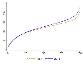
Figure 2: Distribution of Individual Earnings

Figure 2 displays the distribution of annual earnings in the SSA, replicating Figure I in Song, Price, Guvenen, Bloom, and Von Wachter (2019). The figure shows individual earnings levels, on the $y$-axis in thousands of dollars, for each percentile of the income distribution, on the $x$-axis.

Figure 2 shows individual earnings by percentile of the earnings distribution for 1981 and 2013. In 1981, earnings vary between 18 thousand at the 25th percentile, to 31 thousand at the median, to 89 thousand at the 95th percentile. By 2013, earnings are 19 thousand at the 25th percentile, 35 thousand at the median, and 132 thousand at the 95th percentile. Figure 2 shows that the earnings distribution features considerable dispersion in levels, which has increased over time. Between 1981 and 2013, earnings in the bottom third of the earnings distribution have seen little change, while earnings at the top strongly increased.

We decompose the overall variance of log earnings into within- and between-firm components. Let $w_{ij}$ be log earnings of worker $i$ at firm $j$. Earnings can be written as $w_{ij}=\bar{w}_{j}+(w_{ij}-\bar{w}_{j})$, where $\bar{w}_{j}$ is average log earnings within firm $j$. The total variance is then:

$$\text{Var}(w_{ij})=\text{Var}(\bar{w}_{j})+\sum_{j}\theta_{j}\text{Var}(w_{ij}|i\in j)\hskip 1.9919pt,$$ (22)

where $\theta_{j}$ is the employment share of firm $j$. The first term is the variance of mean earnings across firms, or the between-firm variance. The second term is the average of within-firm dispersion of employee earnings weighted by employment.

The variance of log earnings in 1981, 0.65 log points, is for one-third attributed to differences in mean earnings between firms and for two-thirds to within-firm earnings dispersion as documented by Song, Price, Guvenen, Bloom, and Von Wachter (2019). From 1981 to 2013 the variance of log earnings increased by 0.20 log points to 0.85. Two-thirds of this increase is attributed to increased differences in mean earnings across firms, while a third is attributed to an increase in within-firm earnings dispersion.

5.2 Model

We assess the ability of our model to generate dispersion in earnings, its decomposition between and within firms, as well as changes in the distribution of earnings over time. We then use the calibrated model to structurally decompose increased earnings dispersion between changes on the worker side and changes on the firm side of the labor market.

In our model, the worker skill distribution $F_{x}$ and the project value distribution $F_{z}$ are both exogenous. We parameterize the distribution for workers as $\text{Beta}(\alpha_{x},\beta_{x})$ and the distribution for projects as $\text{Beta}(\alpha_{z},\beta_{z})$. We consider teams with two workers.

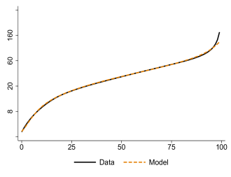
(a) 1981

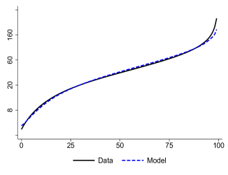
(b) 2013

Figure 3: Data and Model Distribution of Individual Earnings

Figure 3 compares the empirical earnings distribution to the model earnings distribution. The empirical distributions, which we display by solid black lines, follow Figure 2, while the model distributions are presented by dashed lines. The left panel shows the empirical and model distribution for 1981, the right panel for 2013.

We use the cross-sectional distribution of earnings and the decomposition of the earnings variation into within-firm and between-firm variation to inform the worker and project distribution. We estimate the underlying distributions using earnings in the cross-section using the data underlying Figure 2. The resulting model fit for cross-sectional earnings is summarized by Figure 3. Figure 3 shows that our framework generates the observed dispersion in earnings, as well as changes in the distribution of earnings over time while somewhat underestimating earnings at the very top percentiles in both 1981 and 2013.

Table 1: Model and Data Earnings Decomposition

	Data			Model
Moment	1981	2013	change	1981	2013	change
Between	0.34	0.42	0.08	0.34	0.43	0.09
Within	0.66	0.58	-0.08	0.66	0.57	-0.09

Table 1 compares the empirical and model decomposition of earnings dispersion. The left panel shows the empirical decomposition of earnings variation in dispersion between firms and dispersion within firms following (22), while the right panel shows the model analog.

Table 1 displays the decomposition for the variance of log earnings between 1981 and 2013 in the data and the model. Our stylized model can account for the earnings decomposition in 1981. The fifth column shows that the model correctly attributes a third of the earnings variation to dispersion between firms, and two thirds to dispersion within firms. The model generates an increase in the share of the between-firm variance from 0.34 to 0.43 percentage points between 1981 and 2013, while capturing the overall increase in earnings dispersion as shown in Figure 3.

Table 2: Model and Data Coworker Earnings

	Data			Model
Percentile	1981	2013	change	1981	2013	change
25	10.01	10.07	0.06	10.19	10.30	0.11
50	10.30	10.45	0.15	10.44	10.63	0.19
75	10.56	10.75	0.19	10.56	10.83	0.27
90	10.67	10.98	0.31	10.46	10.70	0.24

Table 2 compares the model and data in terms of mean coworker earnings. The left panel shows mean coworker earnings at selected percentiles of the individual earnings distribution. The right panel shows their model analog. All numbers are log points.

In addition to studying the variance decomposition of log earnings, we evaluate non-targeted average log earnings of coworkers at different percentiles of the earnings distribution. The results are in Table 2. Model and data align qualitatively up to the 75th percentile with quantitative deviations of 0.20 log points. At the top of the skill distribution, the data display a stronger positive correlation between worker earnings compared to our more negatively sorted model economy.

5.3 Counterfactual

The rise in earnings dispersion between 1981 and 2013 could be driven by changes in the worker or the firm side of the labor market, or a combination thereof. We use our framework to evaluate the drivers of the increase in earnings dispersion. To do this, we analyze counterfactual changes in earnings dispersion by only changing the worker distribution and by only changing the project value distribution.

Table 3: Model and Data Earnings Decomposition

	Model			Firm Effect		Worker Effect
Moment	1981	2013	change	2013	change	2013	change
Between	0.34	0.42	0.08	0.12	-0.22	0.72	0.38
Within	0.66	0.58	-0.08	0.88	0.22	0.28	-0.38

Table 3 compares the baseline and counterfactual model decomposition of earnings dispersion. The left panel shows the baseline model decomposition of earnings as in Table 1, while the middle and right panel show counterfactual decompositions. For the firm effect counterfactual, we evaluate the model with the worker distribution for 1981 and the firm distribution for 2013, while the worker effect counterfactual evaluates the model using the firm distribution for 1981 and the worker distribution for 2013.

Table 3 shows a structural decomposition of changes in earnings dispersion from 1981 to 2013. The left panel repeats the baseline decomposition, while the middle panel and right panel present counterfactual results. The firm effect counterfactual evaluates the model for the distribution of workers in 1981 and the firm distribution in 2013. The middle panel demonstrates that by only changing the distribution of firm projects, the share of within-firm earnings dispersion would have increased by 22 percentage points. The worker effect counterfactual similarly evaluates the model using the project distribution of 1981 and the worker distribution of 2013. The right panel shows that the share of the within-firm earnings dispersion would have decreased by 38 percentage points. That is, our counterfactual analysis shows that both the changes in the worker and project distributions between 1981 and 2013 are important in the model in generating the observed change in earnings dispersion.

6 Conclusion

We provide a complete solution to an assignment problem with heterogeneous firms and multiple heterogeneous workers whose skills are imperfect substitutes, that is, for a submodular technology.

Sorting with Teams

Appendix

Job Boerma, Aleh Tsyvinski and Alexander Zimin

November 2023

Appendix A Proofs

In this appendix, we formally prove the results in the main text.

A.1 Equilibrium, Planning Problem and Duality

We formally define an equilibrium for the economy.

A firm with project $z$ chooses workers $x_{1},x_{2},\dots,x_{m}$ to maximize profits taking the wage schedule for workers $w$ as given. The firm problem is:

$$v(z)=\max_{\{x_{i}\}}\;y(x_{1},\dots,x_{m},z)-\sum^{m}_{i=1}w(x_{i}).$$ (A.1)

Worker $x_{i}$ chooses to work for firm $z$ with coworkers $\{x_{j}\}$ for $j\neq i$ to maximize their wage income. The worker takes the wage schedule for their coworkers and the firm value $v$ as given:

$$w(x_{i})=\max_{\{x_{j}\},z}\;y(x_{1},x_{2},\dots,x_{m},z)-\sum^{m}_{j\neq i}w(x_{j})-v(z).$$ (A.2)

An equilibrium is a wage function $w$, firm value function $v$, and feasible assignment function $\pi$, such that firms solve their profit maximization problem (A.1), workers solve the worker problem (A.2), and satisfy a feasibility constraint:

$$\int y(x_{1},x_{2},\dots,x_{m},z)\text{d}\pi=\sum_{i=1}^{m}\int w(x_{i})\text{d}F_{x}+\int v(z)\text{d}F_{z},$$ (A.3)

which states that total output produced, $\int y(x_{1},x_{2},\dots,x_{m},z)\text{d}\pi$, equals total output distributed to workers and firms.

We use the following relation between the planning problem and the dual formulation.

Lemma 1.

Let $\pi\in\Pi(F_{x},\dots,F_{x},F_{z})$ be a joint probability measure, and $(w,v)$ be functions such that the surplus $S(x_{1},\dots,x_{m},z)=y(x_{1},\dots,x_{m},z)-\sum w(x_{i})-v(z)\leq 0$ for all $(x_{1},\dots,x_{m},z)$. If there is a set $M\subset X\times\dots\times X\times Z$ such that $S(x_{1},\dots,x_{m},z)=0$ on $M$ with the additional property that $\pi(M)=1$, then assignment $\pi$ is a primal solution and functions $w$ and $v$ are a dual solution.

Since the assignment in Lemma 1 is concentrated on set $M$, we refer to $M$ as the set of potential matches. The proof to Lemma 1 only makes use of a notion of weak duality.

Weak Duality. Let $\pi\in\Pi(F_{x_{1}},\dots,F_{x_{m}},F_{z})$ be a joint probability measure, and $f_{i}\in L^{1}(X,F_{x_{i}})$, $g\in L^{1}(Z,F_{z})$ be integrable functions such that $y(x_{1},\dots,x_{m},z)\leq\sum\limits_{i=1}^{m}f_{i}(x_{i})+g(z)$ for all teams $(x_{1},\dots,x_{m},z)$. Then

$$\min_{\{f_{i}\},g}\;\sum_{i=1}^{m}\int f_{i}(x_{i})\text{d}F_{x_{i}}+\int g(z)\text{d}F_{z}\;\geq\;\max_{\pi\in\Pi}\;\int y(x_{1},\dots,z)\text{d}\pi.$$ (A.4)

Proof.

For any functions $\{f_{i}\}$ and $g$ so that $y(x_{1},\dots,x_{m},z)\leq\sum\limits_{i=1}^{m}f_{i}(x_{i})+g(z)$ we have:

$$\max_{\pi\in\Pi}\int y(x_{1},\dots,x_{m},z)\text{d}\pi\leq\int\Big{(}\sum\limits_{i=1}^{m}f_{i}(x_{i})+g(z)\Big{)}\text{d}\pi=\sum_{i=1}^{m}\int f_{i}(x_{i})\text{d}F_{x_{i}}+\int g(z)\text{d}F_{z},$$

where the equality follows as $\pi\in\Pi(F_{x_{1}},\dots,F_{x_{m}},F_{z})$. Since the inequality holds for any $(\{f_{i}\},g)$ and $g$ it holds for $(\{f_{i}\},g)$ that minimize the right-hand side. ∎

We use weak duality to establish Lemma 1 by contradiction.

Proof of Lemma 1. Suppose by contradiction that $\hat{\pi}$ does not solve the primal problem. Then there exists another probability measure $\pi$ such that

$$\max_{\pi\in\Pi}\int y(x_{1},\dots,x_{m},z)\text{d}\pi >\int y(x_{1},\dots,x_{m},z)\text{d}\hat{\pi}=\sum_{i=1}^{m}\int\hat{f}_{i}(x_{i})\text{d}F_{x_{i}}+\int\hat{g}(z)\text{d}F_{z}$$

$$\hskip 93.60938pt\geq\min_{\{f_{i}\},g}\;\sum_{i=1}^{m}\int f_{i}(x_{i})\text{d}F_{x_{i}}+\int g(z)\text{d}F_{z},$$

where the equality follows by the assumption. This contradicts weak duality (A.4).

Suppose by contradiction that the functions $(\{\hat{f}_{i}\},\hat{g})$ do not solve the dual problem. Then there exists functions $(\{f_{i}\},g)$ such that

$$\min_{\{f_{i}\},g}\;\sum_{i=1}^{m}\int f_{i}(x_{i})\text{d}F_{x_{i}}+\int g(z)\text{d}F_{z} <\sum_{i=1}^{m}\int\hat{f}_{i}(x_{i})\text{d}F_{x_{i}}+\int\hat{g}(z)\text{d}F_{z}$$

$$=\int y(x_{1},\dots,x_{m},z)\text{d}\hat{\pi}\leq\max_{\pi\in\Pi}\int y(x_{1},\dots,x_{m},z)\text{d}\pi,$$

where the equality follows by the assumption. This inequality contradicts weak duality (A.4).

While Lemma 1 connects the planning problem and the dual formulation, it does not connect either to our definition of an equilibrium. The link is Proposition 7.

Proposition 7.

Let $\pi$ solve the planning problem and let $(w,v)$ solve the dual problem. Then, wage schedule $w$, firm value function $v$, and assignment $\pi$ are an equilibrium.

Proof.

The proof follows from the constraints on the dual problem, or $w(x_{i})\geq y(x_{1},\dots,x_{m},z)-\sum\limits_{j\neq i}^{m}w(x_{j})-v(z)$, which imply:

$$w(x_{i})\geq\hskip 0.85355pt\max_{x_{\neg i},z}\Big{(}y(x_{1},\dots,x_{m},z)-\sum\limits_{j\neq i}^{m}w(x_{j})-v(z)\Big{)}.$$ (A.5)

The equality follows since $y(x_{1},\dots,x_{m},z)=\sum\limits_{i=1}^{m}w(x_{i})+v(z)$ on the set of potential matches $M$ on which the assignment function is concentrated. The argument for the firm value function $v$ is identical. The equality also implies that the goods market clears.∎

Proposition 7 implies that assignment function $\pi$, wage schedule $w$, and firm value function $v$ are an equilibrium. Given this connection, we call $w$ the wage schedule and $v$ the firm value.

A.2 Majorization Inequality

We verify the second assumption to the majorization inequality (13). The goal is to show that the mixed an countermonotonic assignment is optimal. We do not require all properties of the mixed and countermonotonic assignment described in Definition 1. Specifically, we prove Proposition 8.

Proposition 8.

Suppose assignment $\pi\in\Pi$ satisfies two conditions. First, the loss of the $1-q$ largest teams are the same. Second, consider the first $t\leq q$ teams. Worker $x_{i}\in F_{i}$ belongs to one of them if and only if $x_{i}\in[0,I_{i}(\underline{t}_{i}(t))]$ or $x_{i}\in[I_{i}(1-\bar{t}_{i}(t)),1]$. Then, $\pi\in\Pi$ solves the planning problem (5).

For any assignment $\pi$, let $S_{\gamma}(t)$ denote the cumulative logarithmic losses for the $t$ teams with the smallest losses:

$$S_{\gamma}(t)=\int_{0}^{t}\log I_{\gamma}(p)\text{d}p.$$ (A.6)

To verify (13) we compare $S_{\gamma^{*}}$ to $S_{\gamma}$.

Suppose there exists a mixed and countermonotonic assignment $\pi^{*}$ with an associated loss distribution $\gamma^{*}$. Next, we prove $S_{\gamma^{*}}$ is the maximal cumulative logarithmic loss in line with the second assumption to the majorization inequality, that is, for any assignment $\pi$, $S_{\gamma^{*}}(t)\geq S_{\gamma}(t)$ for all $t\in[0,1]$. To establish this, we first bound the cumulative logarithmic losses in the countermonotonic sets of $\pi^{*}$ from below.

Lemma 2.

For any feasible assignment $\pi$ and for all $t\in[0,q]$, $S_{\gamma}(t)\leq S_{\gamma^{*}}(t)$.

Proof.

The function $S_{\gamma}$ is the sum of logarithmic losses for the $t$ teams with smallest output losses. For any other set $U$ with mass $\pi(U)=t$, by definition:

$$S_{\gamma}(t)\leq\int\log\ell(x_{1},\dots,x_{m},z)\text{d}\pi_{U}.$$ (A.7)

where $\pi_{U}$ restricts assignment $\pi$ to the set $U$.

Define the set of teams with the $\underline{t}_{k}(t)$ highest skill workers in dimension $k$ as:

$$V_{k}:=\{(x_{1},\dots,x_{m},z)\in[0,1]^{n}\;|\;0\leq x_{k}\leq I_{k}(\underline{t}_{k}(t))\}$$ (A.8)

The measure of the set $V_{k}$ with respect to assignment $\pi$ is $\underline{t}_{k}(t)$. The union of sets $V=V_{1}\cup\dots\cup V_{n}$ thus has measure of at most $t$ with respect to assignment $\pi$. We construct a set $U\supset V$ such that $\pi(U)=t$ by adding some additional set of teams to the set $U$.

Given that $\pi_{U}$ represents the restriction of the assignment function $\pi$ to the specified set $U$, we use (A.7) to write:

$$S_{\gamma}(t)\leq\int\log\ell(x_{1},\dots,x_{m},z)\text{d}\pi_{U}=\sum_{k=1}^{m}\int\log x_{k}\text{dPr}_{x_{k}}(\pi_{U})+\int\log z\text{dPr}_{z}(\pi_{U}),$$

where $\text{Pr}_{x_{k}}$ is the projection of measure $\pi_{U}$ onto the $k$-th dimension. To characterize the upper bound, we bound $\int\log x_{k}\text{dPr}_{x_{k}}(\pi_{U})$. Since $V_{k}\subset U$, the density function that corresponds to measure $\text{Pr}_{x_{k}}(\pi_{U})$ is equal to the skill density $f_{k}(x)$ for all $0\leq x\leq I(\underline{t}_{k}(t))$ and is less than skill density $f_{k}$ otherwise. Hence,

$$\int\log x_{k}\text{dPr}_{x_{k}}(\pi_{U}) \leq\int_{0}^{I_{k}(\underline{t}_{k}(t))}\log(x_{k})f_{k}(x_{k})\,\text{d}x_{k}+\int_{I_{k}(1-\bar{t}_{k}(t))}^{1}\log(x_{k})f_{k}(x_{k})\,\text{d}x_{k}$$

$$=\int_{0}^{\underline{t}_{k}(t)}\log I_{k}(p)\,\text{d}p+\int_{1-\bar{t}_{k}(t)}^{1}\log I_{k}(p)\,\text{d}p.$$

where the inequality follows as the second term on the right-hand side captures the contribution to logarithmic losses by the $\bar{t}_{k}(t)$ lowest skill workers. The equality follows by change of variables. Summing over all $k$ dimensions, we obtain:

$$S_{\gamma}(t)\leq\sum_{k=1}^{n}\Big{(}\int_{0}^{\underline{t}_{k}(t)}\log I_{k}(p)\,dp+\int_{1-\bar{t}_{k}(t)}^{1}\log I_{k}(p)\,dp\Big{)}=S_{\gamma^{*}}(t),$$ (A.9)

which was what we wanted. ∎

Lemma 3.

For any feasible assignments $\gamma$ and for all $t\in[q,1]$,

$$S_{\gamma}(t)\leq S_{\gamma^{*}}(t).$$

Proof.

We first observe that cumulative logarithmic loss $S_{\gamma}$ is a convex function as it is the integral over an increasing function. Since $S_{\gamma}$ is convex, for all $t\in[q,1]$:

$$S_{\gamma}(t)\leq\frac{1-t}{1-q}S_{\gamma}(q)+\frac{t-q}{1-q}S_{\gamma}(1)\leq\frac{1-t}{1-q}S_{\gamma^{*}}(q)+\frac{t-q}{1-q}S_{\gamma^{*}}(1)$$ (A.10)

where the final inequality follows because $S_{\gamma}(q)\leq S_{\gamma^{*}}(q)$ by Lemma 2, and $S_{\gamma}(1)=S_{\gamma^{*}}(1)$ by the verification of first assumption to the majorization inequality.

The integral over logarithmic losses $S_{\gamma^{*}}(t)$ is linear for teams with the highest losses $t\in[q,1]$ by the condition that the loss of the $1-q$ largest teams are the same. Hence, for teams $t\in[q,1]$:

$$S_{\gamma^{*}}(t)=\frac{1-t}{1-q}S_{\gamma^{*}}(q)+\frac{t-q}{1-q}S_{\gamma^{*}}(1)$$ (A.11)

Combining (A.10) and (A.11) the result follows. ∎

We combine Lemma 2 and Lemma 3 to verify the second assumption of the majorization inequality, which concludes the proof.

A.3 Characterization of Mixed and Countermonotonic Assignment

The mixed-and-countermonotonic assignment in Definition 1 may appear general, but in fact, the countermonotonic sets $b_{i}(t)$ fully determine the assignment $\pi$.

First, at each percentile $t\leq q$ in the distribution of output losses, there are $n$ teams: one from each countermonotonic set. The logarithmic output loss at percentile $t\leq q$, which we denote $l(t)$, equals

$$l(t)=m\lambda(t)+\sum_{i=1}^{n}\log I_{i}(\underline{t}_{i}(t)).$$ (A.12)

where $\lambda(t)$ is the skill gap between the high-skill and low-skill worker that are in teams at percentile $t\leq q$, which is identical across distributions $i$:

$$\lambda(t)=\log I_{i}(1-\bar{t}_{i}(t))-\log I_{i}(\underline{t}_{i}(t)).$$ (A.13)

Since the functions $I_{i}$, $\underline{t}_{i}$, and $\bar{t}_{i}$ are continuous, the functions $\lambda$ and $l$ are continuous too. It follows from the definition of $l$ that the logarithmic loss function is increasing.

Next, we connect the functions $\underline{t}_{i}$ and $\bar{t}_{i}$. Teams in the countermonotonic sets have low output losses and pair a single low value from one distribution with high values from the remaining distributions. Since the quality of the high-skill worker decreases with team loss percentile $t$, that is, $\underline{t}_{i}(t)$ increases from $\underline{t}_{i}(0)=0$, it follows that the $t$ teams with the lowest losses draw a single high-skill worker from each distribution, so that for $t\leq q$:

$$\underline{t}_{1}(t)+\dots+\underline{t}_{n}(t)=t.$$ (A.14)

Equivalently, high values from the $i$-th distribution, starting from $\bar{t}_{i}(t)=0$, are paired into teams with low values in the remaining countermonotonic sets. Thus, for $t\leq q$:

$$\bar{t}_{i}(t)=\sum\limits_{j\neq i}\underline{t}_{j}(t)=t-\underline{t}_{i}(t).$$ (A.15)

where the final equality follows from (A.14).

Finally, we consider the part of the assignment $\pi$ that is located on the mixed set. Given functions $\{\underline{t}_{i}\}^{n}$, we define for $x\in[0,q]$, the average logarithmic loss for mediocre workers and jobs $h(x)=\frac{1}{1-x}\sum\int_{\underline{t}_{i}(x)}^{\bar{t}_{i}(x)}\log I_{i}(t)\text{d}t$. By construction, the logarithmic loss of any team located on mixed set $B$ is the same and equal to $h(q)$. We can compute it directly:

$$l(q)=\frac{1}{1-q}\int_{B}\log x_{1}\dots x_{m}z\text{d}\pi=\frac{1}{1-q}\sum_{k=1}^{n}\int_{\underline{p}_{k}}^{\bar{p}_{k}}\log x_{k}\,\text{d}F_{k}(x_{k})=h(q).$$ (A.16)

This equation asserts continuity of the assignment: the output loss of teams at the end of countermonotonic sets, $l(q)$, equals the loss of teams located on the mixed set, $h(q)$.

If a mixed and countermonotonic assignment exists, then equations (A.12) to (A.16) are satisfied. Together with the ability to mix mediocre workers and projects, (A.12) to (A.16) are in fact sufficient to show that a mixed and countermonotonic assignment exists as we show in Proposition 9.

Proposition 9.

Consider continuous non-negative increasing functions $\{\underline{t}_{i}\}^{n}_{i=1}$ and a mass $0\leq q\leq 1$ which is located on the countermonotonic sets. There exists a mixed and countermonotonic assignment defined by these functions if and only if

1. For each $t\in[0,q]$, $\underline{t}_{1}(t)+\dots+\underline{t}_{n}(t)=t$ (A.14);

2. For each $t\in[0,q]$, $\bar{t}_{i}(t)=t-\underline{t}_{i}(t)$ are non-negative and increasing (A.15);

3. For each $t\in[0,q]$, the skill gap between the high-skill and low-skill worker $\lambda(t)=\log I_{i}(1-\bar{t}_{i}(t))-\log I_{i}(\underline{t}_{i}(t))$ is independent of $i$ (A.13);

4. For each $t\in[0,q]$, the function $l(t)=m\lambda(t)+\sum\limits_{i=1}^{n}\log I_{i}(\underline{t}_{i}(t))$ is increasing in $t$ (A.12);

5. $h(q)=l(q)$ (A.16);

6. The restriction of $\{F_{i}\}^{n}_{i=1}$ to the intervals $[I_{i}(\underline{t}_{i}(q)),I_{i}(1-\bar{t}_{i}(q))]$ is mixable.

Proof.

To prove Proposition 9 it remains to be shown that if Conditions 1 to 6 apply, then there exists a mixed and countermonotonic assignment defined by the functions $\{\underline{t}_{i}\}$ and a mass $q$ located on countermonotonic sets. The proof is split into two parts. First, we construct the assignment $\pi$ associated with $\{\underline{t}_{i}\}$ and show that it is feasible. Second, we show that assignment $\pi$ is a mixed and countermonotonic assignment. While the result is rather intuitive, this technical proof verifies this formally.

We construct the mixed and countermonotonic assignment completely using the functions $\{\underline{t}_{i}\}$ and the mass $q$ located on the countermonotonic sets. To understand that the assignment is fully determined, first observe that we can construct the increasing functions $\{\bar{t}_{i}\}$ by (A.15). Given the functions $\{\underline{t}_{i},\bar{t}_{i}\}$ and a mass $q$, we use the definition of countermonotonic sets in Definition 1 to construct countermonotonic sets.

We next identify the threshold percentiles $\bar{p}_{i}$ and $\underline{p}\vphantom{p}_{i}$ and show that these threshold percentiles are inside the unit interval. We denote $\underline{p}\vphantom{p}_{i}=\underline{t}_{i}(q)$ and $\bar{p}_{i}=1-\bar{t}_{i}(q)=\underline{p}\vphantom{p}_{i}+(1-q)$, where the second equality follows from equation (A.15) evaluated at $t=q$. The threshold $\underline{p}\vphantom{p}_{i}$ is non-negative since $\underline{t}_{i}$ is a non-negative function, which also implies that $\bar{p}_{i}=\underline{p}\vphantom{p}_{i}+(1-q)$ is non-negative. Next, since $\bar{t}_{i}(q)\geq 0$ by (A.15) it implies that $\bar{p}_{i}\leq 1$, and therefore $\underline{p}\vphantom{p}_{i}=\bar{p}_{i}-(1-q)\leq 1$. Hence, both $\underline{p}\vphantom{p}_{i}$ and $\bar{p}_{i}$ are thresholds inside the unit interval.

Given the threshold percentiles $\{\underline{p}\vphantom{p}_{i},\bar{p}_{i}\}$, we know the support of the mixed set. So far, this procedure only suggests a support of an assignment. A key step is to show there exists a measure concentrated on this support.

The first step in showing there exists a measure concentrated on the suggested support is to reparameterize the countermonotonic set $b_{i}(t)$ from percentiles in the distribution of team losses $t$ to percentiles in the distribution of the $i$-th worker, which we here denoted by $q_{i}$. Since the function $\underline{t}_{i}$ is increasing, its inverse $\underline{t}^{-1}_{i}$ is well-defined. Function $\underline{t}_{i}(t)$ takes percentile $t$ of team losses and returns the percentile of the worker in the $i$-th distribution that is part of this team. The inverse function takes the percentile of the worker in the $i$-th distribution and returns the percentile in the distribution of team losses. This percentile can thus directly be substituted into the definition of a countermonotonic set $b_{i}$. For each $i$, we formally consider the mapping

$$\tilde{b}_{i}(q_{i})=b_{i}(\underline{t}^{-1}_{i}(q_{i})),$$

where $q_{i}\in[0,\underline{p}\vphantom{p}_{i}]$ and $b_{i}$ is the countermonotonic set defined in Definition 1.

Let $\lambda_{i}$ be the Lebesgue measure restricted to the interval $[0,\underline{p}\vphantom{p}_{i}]$, that is, all high-skill workers in distribution $i$ up to percentile $\underline{p}\vphantom{p}_{i}$. Define the corresponding countermonotonic set assignment $\pi_{i}$ as the push-forward image of the measure $\lambda_{i}$ under the mapping $q_{i}\to\tilde{b}_{i}(q_{i})$. We take $\{\lambda_{i}\}^{n}_{i=1}$ and will then analyze the corresponding marginal distributions of these countermonotonic sets $\pi_{b}=\pi_{1}+\dots+\pi_{n}$. First, we find $\tilde{b}_{ii}(q)$:

$$\tilde{b}_{ii}(q)=b_{ii}(\underline{t}^{-1}_{i}(q))=I_{i}\big{(}\underline{t}_{i}\big{(}\underline{t}^{-1}_{i}(q)\big{)}\big{)}=I_{i}(q),$$ (A.17)

where the second equality follows by definition of $b_{ii}$ in Definition 1. In words, the $i$-th marginal distribution of assignment $\pi_{i}$ is the push-forward image of the uniform measure on $[0,\underline{p}\vphantom{p}_{i}]$ under the mapping $x\to I_{i}(x)$, which is the distribution $F_{i}$ restricted to the interval $[0,I_{i}(\underline{p}\vphantom{p}_{i})]$.

How many low skill workers are taken by the countermonotonic sets? We assign low skill workers when we construct countermonotonic sets corresponding to the high skill workers in the remaining distributions. We next calculate how many low skill workers from distribution $k$ are assigned according to the assignment function.

For each percentile $s_{k}\in[\bar{p}_{k},1]$ among the low skill workers in the marginal distribution of worker $k$, we find the measure of the set $S_{k}=\{x\in[0,1]^{n}\mid x_{k}\geq I_{k}(s_{k})\}$ with respect to the measure $\pi_{i}$ for some $i\neq k$. In words, how many low-skilled workers from the $k$-th distribution $x_{k}\geq I_{k}(s_{k})$ are taken by countermonotonic set $\pi_{i}$. First, since the function $\bar{t}_{k}$ is increasing from $0$ to $1-\bar{p}_{k}$ by (A.15), its inverse $\bar{t}_{k}^{-1}$ is well-defined on the interval $[0,1-\bar{p}_{k}]$. We can thus write:

$$x_{k}=\tilde{b}_{ik}(q_{i})=b_{ik}(\underline{t}^{-1}_{i}(q_{i}))\geq I_{k}(s_{k}) \Longleftrightarrow I_{k}\big{(}1-\bar{t}_{k}(\underline{t}_{i}^{-1}(q_{i}))\big{)}\geq I_{k}(s_{k})\Longleftrightarrow\bar{t}_{k}\big{(}\underline{t}_{i}^{-1}(q_{i})\big{)}\leq 1-s_{k}$$

$$\Longleftrightarrow q_{i}\leq\underline{t}_{i}\big{(}\bar{t}_{k}^{-1}(1-s_{k})\big{)}.$$

where $q_{i}$ is again the percentile of the high-shill workers from the $i$-th distribution, and the second equality follows (A.17). Worker $x_{k}$ is in the set of lowest skill workers if we are looking at a percentile $q_{i}$ that satisfies the final inequality. This means that the measure of $S_{k}$ with respect to $\pi_{i}$ is equal to $\underline{t}_{i}(\bar{t}_{k}^{-1}(1-s_{k}))$. Thus, the measure of $S_{k}$ with respect to $\pi_{b}$ is:

$$\pi_{b}(S_{k})=\sum_{i\neq k}\underline{t}_{i}\big{(}\bar{t}_{k}^{-1}\big{(}1-s_{k}\big{)}\big{)}=\bar{t}_{k}\big{(}\bar{t}_{k}^{-1}(1-s_{k})\big{)}=1-s_{k}.$$

where the second equality follows from the definition of $\bar{t}_{k}$ in equation (A.15). Thus, the $k$-th marginal distribution of $\pi_{b}(S_{k})$ has the same cumulative distribution as $F_{k}$ restricted to $[I_{k}(s_{k}),1]$. For each $s_{k}$, the mass of low-skill workers above the $s_{k}$-th percentile that we assign is exactly $1-s_{k}$. Together with equation A.17 this implies

$$\mathrm{pr}_{i}(\pi_{b})=F_{i}\big{|}_{[0,I_{i}(\underline{p}\vphantom{p}_{i})]\cup[I_{i}(\bar{p}_{i}),1]}.$$ (A.18)

Now, let $\pi_{c}$ be an assignment that pairs mediocre workers in teams with the same total output loss, and denote $\pi=\pi_{b}+\pi_{c}$. Equation A.18 and Condition 6 directly imply that $\pi\in\Pi(\{F_{i}\}^{n}_{i=1})$.

The second part of the proof verifies that the constructed assignment is indeed a mixed and countermonotonic assignment. Given the constructed assignment $\pi$, we check that all properties of the mixed and countermonotonic assignment in Definition 1 are satisfied.

The first property is directly verified since we discussed above that $\bar{p}_{i}=\underline{p}\vphantom{p}_{i}+(1-q)$.

To verify the second property, we validate both the countermonotonic sets and the mixed set. It follows directly from their construction that the countermonotonic sets have the required form. Next, we verify the mixed set. For the verification of the mixed set there are two properties to validate. First, that the values $x_{i}$ are bounded between $I_{i}(\underline{p}\vphantom{p}_{i})$ and $I_{i}(\bar{p}_{i})$ is immediate as these are the mediocre workers and jobs.

Second, we show the mixed teams attain a constant, in particular, $I_{i}(\underline{p}\vphantom{p}_{i})\prod\limits_{j\neq i}I_{j}(\bar{p}_{j})$. To validate that the loss of any team on the mixed set, $L_{B}$, equals this constant, we use the definition of the average logarithmic loss for mediocre workers and jobs $h(x)=\frac{1}{1-x}\sum\int_{\underline{t}_{i}(x)}^{\bar{t}_{i}(x)}\log I_{i}(t)\text{d}t$, we have $\log L_{B}=h(q)$. By the fifth condition (A.16), $h(q)=l(q)$, and by the fourth and third condition, we write:

$$l(q) =\log I_{i}(\underline{t}_{i}(q))+\sum_{j\neq i}\log I_{j}(1-\bar{t}_{j}(q))=\log I_{i}(\underline{p}\vphantom{p}_{i})+\sum_{j\neq i}\log I_{j}(\bar{p}_{j}).$$

Hence we establish the loss on the mixed set attains $I_{i}(\underline{p}\vphantom{p}_{i})\prod\limits_{j\neq i}I_{j}(\bar{p}_{j})$, verifying the second property.

The third property of Definition 1 need not be verified directly as it is implied by the statement of the countermonotonic sets in the second property.

Finally, for each percentile $t$, we find the mass of teams with output losses below that of the team located at point $b_{i}(t)$. The logarithmic loss of this team equals $l(t)$. Since the function $l(t)$ is increasing by (A.12) and $\log L_{B}=l(q)>l(t)$, the logarithmic loss of any team from the mixed set is larger than the logarithmic loss of the team $b_{i}(t)$.

We next find all the teams with a loss below the loss of team $b_{i}(t)$ located on the $i$-th countermonotonic set. The logarithm of the loss of team $b_{i}(x)$ is equal to $l(x)$ by Conditions 3 and 4 in Proposition 9. Since the loss function $l(t)$ is increasing, $l(x)\leq l(t)\Longleftrightarrow x\leq t$. As a result, the mass on the countermonotonic set $b_{i}$ such that $x\leq t$ is equal to $\underline{t}_{i}(t)$. In turn, this implies that the mass of teams with logarithmic losses below the logarithmic loss of $b_{i}(t)$ is $\sum\limits_{i=1}^{n}\underline{t}_{i}(t)=t$, where the equality follows by the first condition in Proposition 9. This means that $b_{i}(t)$ in indeed located at the $t$-th quantile of the teams distribution.∎

A.4 Existence of the Mixed and Countermonotonic Assignment

In this appendix, we establish the existence of a mixed and countermonotonic assignment. We prove our results under Assumption 1.

Assumption 1.

For all $x_{i}$, $x_{i}f_{i}(x_{i})$ is non-decreasing.

To construct the optimal assignment, we find continuous non-negative increasing functions $\{\underline{t}_{i}\}$ and a threshold $q$ satisfying all the conditions of Proposition 9. Conditions 1 and 3 in Proposition 9 can be considered a system of functional equations:

$$t =\underline{t}_{1}(t)+\dots+\underline{t}_{n}(t),$$ (A.14)

$$\lambda(t) =\log I_{i}(1-\bar{t}_{i}(t))-\log I_{i}(\underline{t}_{i}(t))$$ (A.13)

for all $i$. The structure of the proof is as follows. First, we show when the system of functional equations (A.13) and (A.14) has a unique solution. Second, we show this unique solution satisfies the remaining Conditions 4 to 6. That is, Conditions 4 to 6 are then properties of the solution.

To show that the system of functional equations specified by Conditions 1 and 3 has a unique solution, we first introduce new notation to transform the system of equations.

Specifically, we introduce new functions $\tilde{y}_{i}(t)$, which capture the negative logarithmic skills of the high-skilled workers on the $t$-th team located on the $i$-th countermonotonic set:

$$\tilde{y}_{i}(t)=-\log I_{i}(\underline{t}_{i}(t)).$$ (A.19)

Since $0\leq I_{i}\leq 1$, we note $0\leq\tilde{y}_{i}<\infty$. We also introduce the distribution function $\tilde{F}_{i}(x)$, which is defined as the cumulative distribution function of negative logarithmic skills of workers from the $i$-th distribution, or $\tilde{F}_{i}(t):=P(\tilde{y}\leq t)=P(x\geq\exp(-t))=1-F_{i}(\exp(-t))$. Using this, we connect $\tilde{y}_{i}(t)$ to $\underline{t}_{i}(t)$:

$$\underline{t}_{i}(t)=1-\tilde{F}_{i}(\tilde{y}_{i}(t)).$$ (A.20)

which is verified from $\tilde{F}_{i}(t)=1-F_{i}(\exp(-t))$, together with $\tilde{y}_{i}(t)=-\log I_{i}(\underline{t}_{i}(t))$.

With these new functions, we write the system of functional equations (A.13) and (A.14) as:

$$t =\sum_{i=1}^{n}\big{(}1-\tilde{F}_{i}(\tilde{y}_{i}(t))\big{)}$$

$$t =\tilde{F}_{i}\big{(}\tilde{y}_{i}(t)-\lambda(t)\big{)}+\big{(}1-\tilde{F}_{i}(\tilde{y}_{i}(t))\big{)}$$

for all $i$.

Given a unique solution, we write the conditions of Proposition 9 in terms of $\tilde{y}_{i}(t)$. First, we check that $\{\underline{t}_{i}\}$ are increasing functions. First, the functions $\underline{t}_{i}(t)=1-\tilde{F}_{i}(\tilde{y}_{i}(t))$ is non-negative if and only if $\tilde{F}_{i}(\tilde{y}_{i}(t))\leq 1$. Next, $\underline{t}_{i}(t)$ is increasing if and only if $\tilde{F}_{i}(\tilde{y}_{i}(t))$ is decreasing. By the monotonicity of $\tilde{F}_{i}$ this is equivalent to $\tilde{y}_{i}(t)$ is decreasing. We verify that $\tilde{y}_{i}(t)$ decreases in Lemma 4.

The concavity of cumulative distribution functions $\tilde{F}_{i}$ on $[0,\infty)$ is equivalent to $x_{i}f_{i}(x_{i})$ is non-decreasing on $[0,1]$, where $f_{i}$ is the density of the skill distribution. Moreover, it is equivalent to $\tilde{f}_{i}$, the density function of the negative logarithmic skill distribution, is non-increasing on $[0,\infty)$. The distribution function for the negative logarithmic skill $\tilde{x}_{i}$ is related to the distribution for $x_{i}$ through $\tilde{F}_{i}(\tilde{x}_{i})=1-F_{i}(\exp(-\tilde{x}_{i}))$. The distribution function $\tilde{F}_{i}$ then has a corresponding density function:

$$\tilde{f}_{i}(\tilde{x}_{i})=\frac{\text{d}}{\text{d}\tilde{x}_{i}}\tilde{F}_{i}(\tilde{x}_{i})=-\frac{\text{d}}{\text{d}\tilde{x}_{i}}F_{i}(\exp(-\tilde{x}_{i}))=f_{i}(\exp(-\tilde{x}_{i}))\exp(-\tilde{x}_{i}).$$ (A.21)

So, $\tilde{f}_{i}$ is non-increasing is equivalent to $x_{i}f_{i}(x_{i})$ is non-decreasing. Therefore, to prove our results, we use Assumption 1.

Conditions 1 to 3 directly follow since $\{\tilde{y}_{i}\}$ is a solution to the system of functional equations (A.13) and (A.14). To verify the fourth condition, we express the function $l(t)$ in terms of $\tilde{y}_{i}(t)$ using the definition of $\tilde{y}_{i}(t)$ in (A.19):

$$l(t)=m\lambda(t)-\sum_{i=1}^{n}\tilde{y}_{i}(t).$$ (A.22)

The fourth condition holds if and only if the right-hand side of equation (A.22) is increasing for $0\leq t\leq q$. We verify this in Lemma 4.

To verify Condition 5, we rewrite the average logarithmic loss for mediocre workers and jobs $h(x)$ in terms of $\tilde{y}_{i}$:

$$h(x)=\frac{1}{1-x}\sum_{i=1}^{n}\int_{\underline{t}_{i}(x)}^{1-\bar{t}_{i}(x)}\log I_{i}(t)\,\text{d}t=-\frac{1}{1-x}\sum_{i=1}^{n}\int_{\tilde{y}_{i}(x)-\lambda(x)}^{\tilde{y}_{i}(x)}z_{i}\,\text{d}\tilde{F}_{i}(z_{i}).$$

The equality follows by a change of variables as $z_{i}=-\log I_{i}(t)$, which by definition is distributed according to $\tilde{F}_{i}$. By equation (A.19) it follows that $-\log I_{i}(\underline{t}_{i}(x))=\tilde{y}_{i}(x)$ and by the third property of Proposition 9 it follows that $-\log I_{i}(1-\bar{t}_{i}(x))=-\log I_{i}(\underline{t}_{i}(x))-\lambda(x)=\tilde{y}_{i}(x)-\lambda(x)$, thereby giving the new bounds of integration. In sum, the fifth condition, $l(q)=h(q)$, holds if and only if

$$-m\lambda(q)+\sum_{i=1}^{n}\tilde{y}_{i}(q)=\frac{1}{1-q}\sum_{i=1}^{n}\int_{\tilde{y}_{i}(q)-\lambda(q)}^{\tilde{y}_{i}(q)}z\,\text{d}\tilde{F}_{i}(z).$$ (A.23)

Lemma 3.2 in Jakobsons, Han, and Wang (2016) states the following:

Lemma 4.

Suppose all cumulative distribution functions $\tilde{F}_{i}$ are concave on $[0,\infty)$. Let $\{\tilde{y}_{i}\}$ and $\lambda$ solve the system of functional equations (A.13) and (A.14). Denote

$$q=\inf\{q\in[0,1]\colon l(q)\geq h(q)\}$$ (A.24)

Then on the interval $(0,q)$ for each $i$:

• $0<\lambda(t)<\tilde{y}_{i}(t)$

• $\lambda(t)$ and $\tilde{y}_{i}(t)$ are decreasing

• $\tilde{y}_{i}(t)-\lambda(t)$ is increasing

• $l(t)$ is increasing

We use Lemma 4 to establish that the fourth and fifth condition are satisfied. Condition 4 follows from the fourth bullet of Lemma 4. To verify the fifth condition, we consider three different cases. First, suppose the threshold $q$ constructed in Lemma 4 is neither equal to $0$ nor equal to $1$. Then, it follows from continuity of $l$ and $h$ that $l(q)=h(q)$ by the definition of $q$, and hence the fifth condition holds automatically. The second case, where $q=1$, is equivalent to the absence of the mixed set, and hence we do not need to verify Condition 5 and 6 of Proposition 9. Finally, the case $q=0$ is equivalent to the absence of countermonotonic sets. In this case, we only need to check Condition 6.

To demonstrate Condition 6 we prove the existence of an assignment such that the output loss is constant across teams. This loss is represented by:

$$x_{1}\dots x_{n}=\exp\Big{(}-\sum_{i=1}^{n}y_{i}\Big{)}$$ (A.25)

where $y_{i}=-\log x_{i}$ is the negative logarithmic skill of a worker. We can hence equivalently state the mixability condition as there exists an assignment of negative logarithmic skills such that the sum of logarithmic skills across teams remains constant.

To determine the distribution of negative logarithmic skills for mediocre workers, consider the following. The skill distribution is $F_{i}$ confined to the interval $[I_{i}(\underline{t}_{i}(q)),I_{i}(1-\bar{t}_{i}(q))]$. The distribution of negative logarithmic skills is $\tilde{F}_{i}$; the distribution of negative logarithmic skills is thus $\tilde{F}_{i}$ restricted to the interval $[-\log I_{i}(1-\bar{t}_{i}(q)),-\log I_{i}(\underline{t}_{i}(q))]$. Using equations (A.13) and (A.19), $-\log I_{i}(\underline{t}_{i}(q))=\tilde{y}_{i}(q)$ as well as $-\log I_{i}(1-\bar{t}_{i}(x))=\tilde{y}_{i}(x)-\lambda(x)$. Thus, the distribution of negative logarithmic skills $\tilde{F}_{i}$ restricted to the interval $[\tilde{y}_{i}(q)-\lambda(q),\tilde{y}_{i}(q)]$. Finally, the total mass of mediocre workers is the same between all distributions and is equal to $1-q$. We normalize all truncated distributions by this constant to make them probabilistic.

Given the distribution of negative logarithmic skills and the normalization of the truncated distribution, we can write the mixability condition in the following lemma.

Lemma 5.

The mixability condition, Condition 6 of Proposition 9, is satisfied if and only if there exists an assignment, denoted $\tilde{\pi}$, such that:

• The marginal projections of assignment $\tilde{\pi}$ are $\frac{1}{1-q}\tilde{F}_{i}$, which are supported on the intervals $[\tilde{y}_{i}(q)-\lambda(q),\tilde{y}_{i}(q)]$.

• This assignment is supported on the hyperplane defined by $y_{1}+\dots+y_{n}=C$, where $C$ is a constant representing the sum of negative logarithmic skills across teams.

We show mixability under Assumption 1 as discussed above. This assumption implies that each cumulative distribution function $\tilde{F}_{i}$ of negative logarithmic skills is concave over the interval $[0,\infty)$. Given that the density function of a distribution is the derivative of its cumulative distribution function, Assumption 1 means that the density function of negative log skills is non-increasing.

A direct result is that each distribution of negative log skills is supported on the interval $[\tilde{y}_{i}(q)-\lambda(q),\tilde{y}_{i}(q)]$, and that its density function decreases within this interval. Building on this, we introduce Theorem 3.2 of Wang and Wang (2016) which provides necessary and sufficient conditions for mixability under these constraints.

Theorem 10 (Theorem 3.2 of Wang and Wang (2016)).

Let $\{F_{i}\}$ be a collection of probability distributions. If each distribution $F_{i}$ is supported on an interval $[l_{i},r_{i}]$ and has a decreasing density function, then there exists an assignment $\tilde{\pi}$ supported on the hyperplane $\tilde{y}_{1}+\dots+\tilde{y}_{n}=C$ with marginal distributions $\{F_{i}\}$ respectively if and only if for all $i$:

$$(r_{i}-l_{i})+\sum_{j=1}^{n}l_{j}\leq\sum_{j=1}^{n}\int_{l_{j}}^{r_{j}}x_{j}\text{d}F_{j}.$$

For our problem, this result implies that the distributions of negative logarithmic skills of mediocre workers are mixable if and only if the following inequality is satisfied for each $i$:

$$\lambda(q)+\sum_{i=1}^{n}\big{(}\tilde{y}_{i}(q)-\lambda(q)\big{)}\leq\frac{1}{1-q}\sum_{i=1}^{n}\int_{\tilde{y}_{i}(q)-\lambda(q)}^{\tilde{y}_{i}(q)}z_{i}\text{d}\tilde{F}_{i}(z_{i}),$$ (A.26)

since $l_{k}=\tilde{y}_{k}(q)-\lambda(q)$, $r_{k}=\tilde{y}_{k}(q)$, and $F_{k}=\frac{\tilde{F}_{k}}{1-q}$ in our environment. By equation (A.23) we find that this equation holds with equality if $q\in(0,1)$. Under Condition 5 and Assumption 1, all conditions are thus met. When $q=0$, $l(q)\geq h(q)$ by the definition of $q$ in (A.24). Hence, the distributions of negative logarithmic skills of mediocre workers are mixable.

A.5 General Production Functions

We generalize the functional form of the production function.

Generalizing Technology for $n=3$. In the case of two workers, the technology is generalized to additionally incorporate interaction terms between workers and coworkers $x_{1}x_{2}$, workers and firms $x_{1}z$, and coworkers and firms $x_{2}z$. Let the technology be given by:

$$y(x_{1},x_{2},z)=\varphi_{0}+\varphi_{1}x_{1}+\varphi_{2}x_{2}+\varphi_{3}z-\varphi_{12}x_{1}x_{2}-\varphi_{13}x_{1}z-\varphi_{23}x_{2}z-x_{1}x_{2}z,$$ (A.27)

where $\varphi_{ij}$ are non-negative to ensure submodularity.

Proposition 11.

Let the technology $y(x_{1},x_{2},z)$ take the form (A.27). Suppose the distributions of workers and projects, $F_{x}$ and $F_{z}$ respectively, satisfy Assumption 1 whereas $\tilde{x}f_{\tilde{x}}\left(\tilde{x}\right)$ is non-decreasing for $\tilde{x}\in\{x+\varphi_{13},x+\varphi_{23},z+\varphi_{12}\}$. Then a mixed and countermonotonic assignment is optimal.

Proof.

Without loss, we disregard the constant and linear terms in the technology $y(x_{1},x_{2},z)$, as their contribution to the output loss is independent of the assignment. Consequently, we express the technology as:

$$\hat{y}(x_{1},x_{2},z)=-(x_{1}+\varphi_{23})(x_{2}+\varphi_{13})(z+\varphi_{12}).$$

Let $\hat{z}=z+\varphi_{12}$, $\hat{x}_{1}=x_{1}+\varphi_{23}$, and $\hat{x}_{2}=x_{2}+\varphi_{13}$. With these substitutions, the technology function takes its original form $\hat{y}(\hat{x}_{1},\hat{x}_{2},\hat{z})=-\hat{x}_{1}\hat{x}_{2}\hat{z}$.

Given that all $\varphi_{ij}\geq 0$, the shifted variables remain non-negative and are supported on the intervals $[\varphi_{ij},1+\varphi_{ij}]$. Denote the distributions corresponding to these variables respectively as $\hat{F}_{1}$, $\hat{F}_{2}$, and $\hat{F}_{z}$. These distributions satisfy Assumption 1 if and only if the density functions $f_{x}$ and $f_{z}$ of the original skills satisfy the proposition’s stated assumptions. Therefore, invoking Section A.2 to Section A.4, a mixed and countermonotonic assignment $\hat{\pi}\in\Pi(\hat{F}_{1},\hat{F}_{2},\hat{F}_{z})$ exists and solves the assignment problem in this transformed space. The push-forward image of this assignment $\pi$ in the space of variables $(x_{1},x_{2},z)$ provides a solution to the initial problem, completing the proof. ∎

The argument in the proof also implies the following corollary.

Corollary.

Consider technology $y(x_{1},x_{2},x_{1}x_{2},x_{2}z,x_{1}z,x_{1}x_{2}z)$. Suppose its first-order Taylor expansion around the arguments of the function has negative coefficients on each interaction term $(x_{1}x_{2},x_{2}z,x_{1}z,x_{1}x_{2}z)$ to ensure submodularity. Then a mixed and countermonotonic assignment is optimal.

In sum, our results apply to general functions of interactions (single, pairwise, triple) in the first-order sense. The main insight that allows this generalization is the change of variables.

Generalizing Technology with $n$ Distributions. With $n$ distributions, a somewhat different result applies.

Consider a general technology $y(x_{1},\dots,x_{m},z)$ with heterogeneous workers $\{x_{1},\ldots,x_{m}\}$. For ease of notation, let the project value $z$ be denoted as $z=x_{m+1}=x_{n}$. Consider a second-order Taylor expansion of this technology, which is a second-order polynomial in $x_{1},\ldots,x_{n}$, that can be expressed as:

$$y(x_{1},\ldots,x_{n})=a_{0}+\sum_{i=1}^{n}a_{i}x_{i}+\sum_{i=1}^{n}\sum_{j=1}^{n}a_{ij}x_{i}x_{j}.$$ (A.28)

Specifically, consider the case where the matrix $A=\{a_{ij}\}$ has rank one and is elementwise non-positive to ensure submodularity.

Proposition 12.

Consider production technology (A.28) with $\lambda_{i}\geq 0$ and $f_{i}(x_{i})$ is non-increasing. Define transformed skills $\hat{x}_{i}=\exp(-\lambda_{i}x_{i})$, with $\hat{F}_{x_{i}}$ denoting the corresponding distributions of $\hat{x}_{i}$. Then, there exists a mixed and countermonotonic assignment $\hat{\pi}\in\Pi(\hat{F}_{x_{1}},\ldots,\hat{F}_{x_{n}})$ such that its push-forward image in the space of original skills $(x_{1},\ldots,x_{n})$ is an optimal solution.

Proof.

We disregard the constant and linear terms in technology (A.28) as their contribution to the loss is independent of the assignment. Thus, we focus on the technology:

$$\hat{y}(x_{1},\ldots,x_{n})=-\sum_{i=1}^{n}\sum_{j=1}^{n}\lambda_{i}\lambda_{j}x_{i}x_{j}=-\big{(}\sum_{i=1}^{n}\lambda_{i}x_{i}\big{)}^{2}.$$

With $\hat{x}_{i}=\exp(-\lambda_{i}x_{i})$, we write this technology as $\hat{y}(\hat{x}_{1},\ldots,\hat{x}_{n})=-(\sum_{i=1}^{n}\log\hat{x}_{i})^{2}$.

First, we verify that each distribution $\hat{F}_{x_{i}}$ satisfies Assumption 1. Observe that:

$$\hat{f}_{i}(\hat{x}_{i})=\frac{1}{\lambda_{i}\hat{x}_{i}}f_{i}(x_{i}),$$

which implies that the condition $\hat{x}_{i}\hat{f}_{i}(\hat{x}_{i})$ is non-decreasing is equivalent to the density function $f_{i}(x_{i})$ being non-increasing. Thus, by invoking Section A.3 and Section A.4, we deduce the existence of a mixed and countermonotonic assignment $\hat{\pi}\in\Pi(\hat{F}_{x_{1}},\ldots,\hat{F}_{x_{n}})$.

In the proof of optimality for a mixed and countermonotonic assignment, we show using the majorization inequality that the distribution of the sum of logarithmic skills under $\hat{\pi}$, that is, the distribution of $\sum\log\hat{x}_{i}$, is minimal in the sense of second-order stochastic dominance compared to any other assignment $\pi$. Formally, for any convex function $h$ and alternative assignment $\pi$, the inequality

$$\int h\Big{(}\sum_{i=1}^{n}\log\hat{x}_{i}\Big{)}\text{d}\hat{\pi}\leq\int h\Big{(}\sum_{i=1}^{n}\log\hat{x}_{i}\Big{)}\text{d}\pi$$

holds. Taking $h(t)=t^{2}$, we find that $\hat{\pi}$ maximizes total output of the transformed technology $\hat{y}(\hat{x}_{1},\dots,\hat{x}_{n})=-(\sum\log\hat{x}_{i})^{2}$, and the push-forward of assignment $\hat{\pi}$ to the space of original skills $(x_{1},\dots,x_{n})$ solves the initial sorting problem.∎

A.6 Dual Problem

To characterize the solution to the dual problem, we use a generalization of Kantorovich duality for multiple marginal distributions (Kellerer, 1984). The duality result states that the optimal value for the planning problem coincides with the optimal value for the dual problem, and that the dual solution exists in the class of integrable functions.

Duality. Let $X$ and $Z$ be compact subsets of the set of real numbers, and $F_{x}$ and $F_{z}$ be probability measures on $X$ and $Z$ respectively. Let loss function $\ell(x_{1},\dots,x_{m},z)$ be continuous on $X\times\dots\times X\times Z$ and $\Pi(F_{x},\dots,F_{x},F_{z})$ denote the set of measures $\pi$ on $X\times\dots\times X\times Z$ with fixed projections $\text{pr}_{x_{i}}(\pi)=F_{x}$ and $\text{pr}_{z}(\pi)=F_{z}$. Then,

$$\min_{\pi\in\Pi}\int\ell(x_{1},\dots,x_{m},z)\text{d}\pi=\max\sum\limits_{i=1}^{m}\int\hat{w}_{i}(x_{i})\text{d}F_{x}+\int\hat{v}(z)\text{d}F_{z},$$ (A.29)

where the supremum is taken with respect to the collection of integrable functions $\hat{w}_{i}\in L^{1}(X,F_{x})$ and $v\in L^{1}(Z,F_{z})$ subject to the constraint $\sum\limits_{i=1}^{m}\hat{w}_{i}(x_{i})+\hat{v}(z)\leq\ell(x_{1},\dots,x_{m},z)$ for any triplet $(x_{1},\dots,x_{m},z)\in X\times\dots\times X\times Z$.

Applying the duality theorem to our problem, we establish that the dual solution attains the same value as the planning problem and that the dual solution exists in the class of integrable functions. We establish that the solution exists in the class of continuous functions.

Lemma 6.

For any dual solution $(w_{1},\dots,w_{m},v)$, there exist continuous functions $(\hat{w}_{1},\dots,\hat{w}_{m},\hat{v})$ such that $\hat{w}_{i}=w_{i}$ and $\hat{v}=v$ almost everywhere that solves the dual problem.

Proof.

For any dual solution $(w_{1},\dots,w_{m},v)$ we define:

$$\hat{w}_{1}(x_{1}):=\sup_{x_{2},\dots,x_{m},z}\;y(x_{1},\dots,x_{m},z)-\sum\limits_{i=2}^{m}w_{i}(x_{i})-v(z),$$ (A.30)

where $\hat{w}_{1}(x_{1})\leq w_{1}(x_{1})$ since $w_{1}(x_{1})\geq y(x_{1},\dots,x_{m},z)-\sum_{i=2}^{m}w_{i}(x_{i})-v(z)$. By equation (A.30), we also have $\hat{w}_{1}(x_{1})\geq y(x_{1},\dots,x_{m},z)-\sum_{i=2}^{m}w_{i}(x_{i})-v(z)$, or equivalently, $\hat{w}_{1}(x_{1})+\sum_{i=2}^{m}w_{i}(x_{i})+v(z)\geq y(x_{1},\dots,x_{m},z)$ so that $(\hat{w}_{1},w_{2},\dots,w_{n},v)$ is indeed a feasible solution to the dual problem (7). Since through $\hat{w}_{1}(x_{1})\leq w_{1}(x_{1})$, it follows that

$$\int\hat{w}_{1}(x_{1})\text{d}F_{x}+\sum\limits_{i=2}^{m}w_{i}(x_{i})\text{d}F_{x}+\int v(z)\text{d}F_{z}\leq\int w_{1}(x_{1})\text{d}F_{x}+\sum\limits_{i=2}^{m}w_{i}(x_{i})\text{d}F_{x}+\int v(z)\text{d}F_{z}.$$

Thus, $(\hat{w}_{1},w_{2},\dots,w_{m},v)$ is a dual solution. Furthermore, $\hat{w}_{1}=w_{1}$ almost everywhere. Suppose not, then instead $\hat{w}_{1}<w_{1}$, which would imply that:

$$\int\hat{w}_{1}(x_{1})\text{d}F_{x}+\sum\limits_{i=2}^{m}w_{i}(x_{i})\text{d}F_{x}+\int v(z)\text{d}F_{z}<\int w_{1}(x_{1})\text{d}F_{x}+\sum\limits_{i=2}^{m}w_{i}(x_{i})\text{d}F_{x}+\int v(z)\text{d}F_{z}.$$

which would contradict that $(w_{1},\dots,w_{m},v)$ is a dual solution.

We next establish that $\hat{w}_{1}$ is a continuous function. To show this, let $\hat{w}_{1}(x_{1};x_{2},\dots,x_{m},z):=y(x_{1},\dots,x_{m},z)-\sum_{i=2}^{m}w_{i}(x_{i})-v(z)$, that is, (A.30) holding constant all coworkers $(x_{2},\dots,x_{m})$ and the firm $z$. Given the technology (3), and since $x_{i}\in[0,1]$ and $z\in[0,1]$, $\hat{w}_{1}(x_{1};x_{2},\dots,x_{m},z)$ is a linear function in $x_{1}$ with slope less than one in absolute value. This implies $\hat{w}_{1}(x_{1};x_{2},\dots,x_{m},z)$ is Lipschitz continuous. Since $\hat{w}_{1}(x_{1})$ can be represented as $\hat{w}_{1}(x_{1})=\sup\limits_{x_{2},\dots,x_{m},z}\hat{w}_{1}(x_{1};x_{2},\dots,x_{m},z)$, $\hat{w}_{1}(x_{1})$ is Lipschitz continuous as the supremum of uniformly Lipschitz continuous functions is Lipschitz continuous. Hence, $\hat{w}_{1}(x_{1})$ is continuous.

Similarly, we sequentially define $\{\hat{w}_{i}\}$ and $\hat{v}$:

$$\hat{w}_{i}(x_{i}) :=\hskip 6.25963pt\sup_{x_{j\neq i},z}\hskip 3.69899pty(x_{1},\dots,z)-\sum\limits_{j=1}^{i-1}\hat{w}_{j}(x_{j})-\sum\limits_{j=i+1}^{m}w_{j}(x_{j})-v(z),$$

$$\hat{v}(z) :=\sup_{x_{1},\dots,x_{m}}y(x_{1},\dots,z)-\sum\limits_{i=1}^{m}\hat{w}_{i}(x_{i}).$$

By sequentially applying the above argument, we obtain that $(\hat{w}_{1},\dots,\hat{w}_{m},\hat{v})$ is a dual solution with $\hat{w}_{i}=w_{i}$ for all $i$ and $\hat{v}=v$ almost everywhere. Similarly, the same arguments shows that all $\hat{w}_{i}$ and $\hat{v}$ are continuous.∎

A.7 Proposition 4

For any worker $x_{1,0}$ there exist coworkers $\{x_{j,0}\}_{j=2}^{m}$ and a firm $z_{0}$ so that team $(x_{1,0},\dots,x_{m,0},z_{0})$ is contained in the support of an optimal assignment, implying that:

$$w(x_{1,0})+\dots+w(x_{m,0})+v(z_{0})=y(x_{1,0},\dots,x_{m,0},z_{0})=z_{0}+x_{1,0}m_{x}(x_{1,0}),$$

with the second equality following from the marginal worker product (4). For any other worker $x_{1}$, it must by the constraint be that $w(x_{1})+\dots+w(x_{m,0})+v(z_{0})\geq z_{0}+x_{1}m(x_{1,0})$. Combining these expressions, it holds that for any $x_{0}$ and $x_{1}\in[0,1]$:

$$w(x_{1})-w(x_{1,0})\geq m(x_{1,0})(x_{1}-x_{1,0}).$$ (A.31)

Similarly, by interchanging $x_{1,0}$ and $x_{1}$ in the previous paragraph, we obtain:

$$w(x_{1,0})-w(x_{1})\geq m(x_{1})(x_{1,0}-x_{1}).$$ (A.32)

Combining (A.31) and (A.32), dividing by $(x_{1}-x_{1,0})$ yields

$$m(x_{1})\geq\frac{w(x_{1})-w(x_{1,0})}{x_{1}-x_{1,0}}\geq m(x_{1,0}).$$ (A.33)

Taking limits as $x_{1}\rightarrow x_{1,0}$, this equation shows that the function $w(x)$ has a derivative at $x_{1}=x_{1,0}$ and that this derivative is equal to $m(x_{1,0})$. Since the marginal worker product $m$ is a continuous function by Proposition 3, the derivative of $w$ is continuous. The result is similarly established for $v^{\prime}(z)$.

A.8 Quantitative Robustness and Extensions

The quantitative analysis in the main text assumes that teams are of size three – two workers and a project. In this appendix, we demonstrate that our model can also account for the decomposition of earnings variation within and across firms with teams of sizes four, five, and six. We also find that the non-targeted average coworker earnings are robust to team size. As the number of team members increases, the firm and worker effect become more muted. These results are summarized in Table A.1, Table A.2, and Table A.3.

Table A.1: Parametric Identification with Three Workers

Model and Data Earnings Decomposition
	Data			Model
Moment	1981	2013	change	1981	2013	change
Between	0.34	0.42	-0.08	0.34	0.42	-0.08
Within	0.66	0.58	-0.08	0.66	0.58	-0.08
Model and Data Coworker Earning
	Data			Model
Percentile	1981	2013	change	1981	2013	change
25	10.01	10.07	0.06	10.19	10.28	0.09
50	10.30	10.45	0.15	10.44	10.61	0.17
75	10.56	10.75	0.19	10.56	10.79	0.23
90	10.67	10.98	0.31	10.55	10.82	0.27

Model and Data Earnings Decomposition
	Model		Firm Effect		Worker Effect
Moment	1981	2013	2013	change	2013	change
Between	0.34	0.42	0.24	-0.10	0.52	-0.18
Within	0.66	0.58	0.76	-0.10	0.48	-0.18

Table A.2: Parametric Identification with Four Workers

Model and Data Earnings Decomposition
	Data			Model
Moment	1981	2013	change	1981	2013	change
Between	0.34	0.42	-0.08	0.34	0.42	-0.08
Within	0.66	0.58	-0.08	0.66	0.58	-0.08
Model and Data Coworker Earning
	Data			Model
Percentile	1981	2013	change	1981	2013	change
25	10.01	10.07	0.06	10.24	10.28	0.04
50	10.30	10.45	0.15	10.45	10.62	0.17
75	10.56	10.75	0.20	10.52	10.77	0.25
90	10.67	10.98	0.31	10.50	10.79	0.29

Model and Data Earnings Decomposition
	Model		Firm Effect		Worker Effect
Moment	1981	2013	2013	change	2013	change
Between	0.34	0.42	0.22	-0.12	0.49	-0.15
Within	0.66	0.58	0.78	-0.12	0.51	-0.15

Table A.3: Parametric Identification with Five Workers

Model and Data Earnings Decomposition
	Data			Model
Moment	1981	2013	change	1981	2013	change
Between	0.34	0.42	-0.08	0.34	0.42	-0.08
Within	0.66	0.58	-0.08	0.66	0.58	-0.08
Model and Data Coworker Earning
	Data			Model
Percentile	1981	2013	change	1981	2013	change
25	10.01	10.07	0.06	10.20	10.28	0.08
50	10.30	10.45	0.15	10.43	10.62	0.19
75	10.56	10.75	0.19	10.52	10.76	0.24
90	10.67	10.98	0.31	10.51	10.79	0.28

Model and Data Earnings Decomposition
	Model		Firm Effect		Worker Effect
Moment	1981	2013	2013	change	2013	change
Between	0.34	0.42	0.38	-0.04	0.38	-0.04
Within	0.66	0.58	0.62	-0.04	0.62	-0.04

References

- (1)
- Ahlin (2015) Ahlin, C. (2015): “The Role of Group Size in Group Lending,” Journal of Development Economics, 115, 140–155.
- Ahlin (2017) (2017): “Matching Patterns when Group Size Exceeds Two,” American Economic Journal: Microeconomics, 9(1), 352–84.
- Alkan (1988) Alkan, A. (1988): “Nonexistence of Stable Threesome Matchings,” Mathematical Social Sciences, 16(2), 207–209.
- Becker (1973) Becker, G. S. (1973): “A Theory of Marriage: Part I,” Journal of Political Economy, 81(4), 813–846.
- Bernard, Jiang, and Wang (2014) Bernard, C., X. Jiang, and R. Wang (2014): “Risk Aggregation with Dependence Uncertainty,” Insurance: Mathematics and Economics, 54, 93–108.
- Boerma, Tsyvinski, Wang, and Zhang (2023) Boerma, J., A. Tsyvinski, R. Wang, and Z. Zhang (2023): “Composite Sorting,” NBER Working Paper No. 31656.
- Carlier and Ekeland (2010) Carlier, G., and I. Ekeland (2010): “Matching for Teams,” Economic Theory, 42(2), 397–418.
- Chade and Eeckhout (2018) Chade, H., and J. Eeckhout (2018): “Matching Information,” Theoretical Economics, 13(1), 377–414.
- Chade, Eeckhout, and Smith (2017) Chade, H., J. Eeckhout, and L. Smith (2017): “Sorting through Search and Matching Models in Economics,” Journal of Economic Literature, 55(2), 493–544.
- Chiappori, McCann, and Pass (2017) Chiappori, P.-A., R. J. McCann, and B. Pass (2017): “Multi-to One-Dimensional Optimal Transport,” Communications on Pure and Applied Mathematics, 70(12), 2405–2444.
- Chiappori and Salanié (2016) Chiappori, P.-A., and B. Salanié (2016): “The Econometrics of Matching Models,” Journal of Economic Literature, 54(3), 832–61.
- Chiappori, Salanié, and Weiss (2017) Chiappori, P.-A., B. Salanié, and Y. Weiss (2017): “Partner Choice, Investment in Children, and the Marital College Premium,” American Economic Review, 107(8), 2109–67.
- Dupuy and Galichon (2014) Dupuy, A., and A. Galichon (2014): “Personality Traits and the Marriage Market,” Journal of Political Economy, 122(6), 1271–1319.
- Eeckhout (2018) Eeckhout, J. (2018): “Sorting in the Labor Market,” Annual Review of Economics, 10, 1–29.
- Eeckhout and Kircher (2018) Eeckhout, J., and P. Kircher (2018): “Assortative Matching with Large Firms,” Econometrica, 86(1), 85–132.
- Embrechts, Puccetti, Rüschendorf, Wang, and Beleraj (2014) Embrechts, P., G. Puccetti, L. Rüschendorf, R. Wang, and A. Beleraj (2014): “An Academic Response to Basel 3.5,” Risks, 2(1), 25–48.
- Gaffke and Rüschendorf (1981) Gaffke, N., and L. Rüschendorf (1981): “On a Class of Extremal Problems in Statistics,” Mathematische Operationsforschung und Statistik: Series Optimization, 12(1), 123–135.
- Galichon (2018) Galichon, A. (2018): Optimal Transport Methods in Economics. Princeton University Press.
- Galichon and Salanié (2021) Galichon, A., and B. Salanié (2021): “Cupid’s Invisible Hand: Social Surplus and Identification in Matching Models,” New York University Working Paper.
- Gangbo and Świech (1998) Gangbo, W., and A. Świech (1998): “Optimal Maps for the Multidimensional Monge-Kantorovich Problem,” Communications on Pure and Applied Mathematics, 51(1), 23–45.
- Garicano (2000) Garicano, L. (2000): “Hierarchies and the Organization of Knowledge in Production,” Journal of Political Economy, 108(5), 874–904.
- Garicano and Rossi-Hansberg (2004) Garicano, L., and E. Rossi-Hansberg (2004): “Inequality and the Organization of Knowledge,” American Economic Review Papers & Proceedings, 94(2), 197–202.
- Garicano and Rossi-Hansberg (2006) (2006): “Organization and Inequality in a Knowledge Economy,” Quarterly Journal of Economics, 121(4), 1383–1435.
- Garicano and Rossi-Hansberg (2015) (2015): “Knowledge-Based Hierarchies: Using Organizations to Understand the Economy,” Annual Review of Economics, 7(1), 1–30.
- Gavilan (2012) Gavilan, A. (2012): “Wage Inequality, Segregation by Skill and the Price of Capital in an Assignment Model,” European Economic Review, 56(1), 116–137.
- Gladkov and Zimin (2020) Gladkov, N. A., and A. P. Zimin (2020): “An Explicit Solution for a Multimarginal Mass Transportation Problem,” SIAM Journal on Mathematical Analysis, 52(4), 3666–3696.
- Gretsky, Ostroy, and Zame (1992) Gretsky, N. E., J. M. Ostroy, and W. R. Zame (1992): “The Nonatomic Assignment Model,” Economic Theory, 2, 103–127.
- Hardy, Littlewood, and Pólya (1929) Hardy, G. H., J. E. Littlewood, and G. Pólya (1929): “Some Simple Inequalities Satisfied by Convex Functions,” Messenger of Mathematics, 58, 145–152.
- Herkenhoff, Lise, Menzio, and Phillips (2023) Herkenhoff, K., J. Lise, G. Menzio, and G. M. Phillips (2023): “Production and Learning in Teams,” NBER Working Paper No. 25179.
- Jakobsons, Han, and Wang (2016) Jakobsons, E., X. Han, and R. Wang (2016): “General Convex Order on Risk Aggregation,” Scandinavian Actuarial Journal, 2016(8), 713–740.
- Jarosch, Oberfield, and Rossi-Hansberg (2021) Jarosch, G., E. Oberfield, and E. Rossi-Hansberg (2021): “Learning From Coworkers,” Econometrica, 89(2), 647–676.
- Kantorovich (1942) Kantorovich, L. V. (1942): “On the Translocation of Masses,” in Dokl. Akad. Nauk. USSR, vol. 37, pp. 227–229.
- Karamata (1932) Karamata, J. (1932): “Sur une Inégalité Relative aux Fonctions Convexes,” Publications Mathématiques de l’Université de Belgrade, 1(1), 145–147.
- Kellerer (1984) Kellerer, H. G. (1984): “Duality Theorems for Marginal Problems,” Zeitschrift für Wahrscheinlichkeitstheorie und Verwandte Gebiete, 67(4), 399–432.
- Kelso and Crawford (1982) Kelso, A. S., and V. P. Crawford (1982): “Job Matching, Coalition Formation, and Gross Substitutes,” Econometrica, 50(6), 1483–1504.
- Kim and Pass (2014) Kim, Y.-H., and B. Pass (2014): “A General Condition for Monge Solutions in the Multi-Marginal Optimal Transport Problem,” SIAM Journal on Mathematical Analysis, 46(2), 1538–1550.
- Knott and Smith (2006) Knott, M., and C. Smith (2006): “Choosing Joint Distributions so that the Variance of the Sum is Small,” Journal of Multivariate Analysis, 97(8), 1757–1765.
- Kremer and Maskin (1996) Kremer, M., and E. Maskin (1996): “Wage Inequality and Segregation by Skill,” NBER Working Paper No. 5718.
- Lindenlaub (2017) Lindenlaub, I. (2017): “Sorting Multidimensional Types: Theory and Application,” Review of Economic Studies, 84(2), 718–789.
- Lindenlaub and Postel-Vinay (2020) Lindenlaub, I., and F. Postel-Vinay (2020): “Multidimensional Sorting under Random Search,” Yale University Working Paper.
- McCann, Shi, Siow, and Wolthoff (2015) McCann, R. J., X. Shi, A. Siow, and R. Wolthoff (2015): “Becker meets Ricardo: Multisector Matching with Communication and Cognitive skills,” Journal of Law, Economics, and Organization, 31(4), 690–720.
- Monge (1781) Monge, G. (1781): “Mémoire sur la Théorie des Déblais et des Remblais,” Histoire de l’Académie Royale des Sciences de Paris, pp. 666–704.
- Ocampo Díaz (2022) Ocampo Díaz, S. (2022): “A Task-Based Theory of Occupations with Multidimensional Heterogeneity,” Western University Working Paper.
- Pass (2011) Pass, B. (2011): “Uniqueness and Monge Solutions in the Multimarginal Optimal Transportation Problem,” SIAM Journal on Mathematical Analysis, 43(6), 2758–2775.
- Pečarić (1984) Pečarić, J. E. (1984): “On Some Inequalities for Functions with Nondecreasing Increments,” Journal of Mathematical Analysis and Applications, 98(1), 188–197.
- Puccetti and Wang (2015) Puccetti, G., and R. Wang (2015): “Extremal Dependence Concepts,” Statistical Science, 30(4), 485–517.
- Quint (1991) Quint, T. (1991): “The Core of An m-Sided Assignment Game,” Games and Economic Behavior, 3(4), 487–503.
- Rachev and Rüschendorf (1998) Rachev, S. T., and L. Rüschendorf (1998): Mass Transportation Problems: Volume I: Theory. Springer Science and Business.
- Rüschendorf and Uckelmann (2002) Rüschendorf, L., and L. Uckelmann (2002): “Variance Minimization and Random Variables with Constant Sum,” in Distributions with Given Marginals and Statistical Modelling, ed. by C. M. Cuadras, J. Fortiana, and J. A. Rodriguez-Lallena.
- Saint-Paul (2001) Saint-Paul, G. (2001): “On the Distribution of Income and Worker Assignment under Intrafirm Spillovers, with an Application to Ideas and Networks,” Journal of Political Economy, 109(1), 1–37.
- Sattinger (1993) Sattinger, M. (1993): “Assignment Models of the Distribution of Earnings,” Journal of Economic Literature, 31(2), 831–880.
- Sherstyuk (1999) Sherstyuk, K. (1999): “Multisided Matching Games with Complementarities,” International Journal of Game Theory, 28, 489–509.
- Song, Price, Guvenen, Bloom, and Von Wachter (2019) Song, J., D. J. Price, F. Guvenen, N. Bloom, and T. Von Wachter (2019): “Firming Up Inequality,” Quarterly Journal of Economics, 134(1), 1–50.
- Wang and Wang (2011) Wang, B., and R. Wang (2011): “The Complete Mixability and Convex Minimization Problems with Monotone Marginal Densities,” Journal of Multivariate Analysis, 102(10), 1344–1360.
- Wang and Wang (2016) (2016): “Joint Mixability,” Mathematics of Operations Research, 41(3), 808–826.