Screening the Discrepancy Function of a Computer Model

Abstract

Screening traditionally refers to the problem of detecting active inputs in the computer model. In this paper, we develop methodology that applies to screening, but the main focus is on detecting active inputs not in the computer model itself but rather on the discrepancy function that is introduced to account for model inadequacy when linking the computer model with field observations. We contend this is an important problem as it informs the modeler which are the inputs that are potentially being mishandled in the model, but also along which directions it may be less recommendable to use the model for prediction. The methodology is Bayesian and is inspired by the continuous spike and slab prior popularized by the literature on Bayesian variable selection. In our approach, and in contrast with previous proposals, a single MCMC sample from the full model allows us to compute the posterior probabilities of all the competing models, resulting in a methodology that is computationally very fast. The approach hinges on the ability to obtain posterior inclusion probabilities of the inputs, which are very intuitive and easy to interpret quantities, as the basis for selecting active inputs. For that reason, we name the methodology PIPS — posterior inclusion probability screening.

Keywords: Screening, variable selection, computer model, Gaussian process, model discrepancy

1 Introduction

Understanding the world and the complex processes that take place in it has always been a challenge for human beings. Centuries and centuries of scientific research and experiments have increased our knowledge, allowing us to model some of these processes. Here, by modeling we mean that researchers have been able to put together mathematical and/or statistical formulas combining parameters and variables in order to explain the mechanics of a phenomenon of interest.

In this work, we focus on the improvement of mathematical models, also known as computer models, that is, scientific models that are used to understand and explore real phenomena. Often, because of their complexity, these models are implemented in computer programs. Only deterministic models are within the scope of the methodology that we propose.

A computer model only reflects our (always limited) knowledge of the real phenomenon. Hence, an important issue lies in the validation of the model, a process that relies on the confrontation of the model with field data representing possibly noisy measurements of the real phenomenon (Bayarri et al., 2007a). In this scenario, the sources of uncertainty are multiple (Kennedy and O’Hagan, 2001). To name but a few: noise on the field measurements, unknown settings for some parameters included in the computer model or the inadequacy between the computer model and the reality.

The last one, also known as the discrepancy or the bias of the computer model, is usually incorporated within the statistical framework that links the field data with the computer model. Moreover, it is commonly modeled as a Gaussian Stochastic Process (GaSP) (Kennedy and O’Hagan, 2001; Higdon et al., 2004; Bayarri et al., 2007b), leading to additional difficulties and potential to confounding issues (Tuo and Wu, 2015) with the estimation of the unknown model parameters, known as the calibration task. Some proposals have been made to use prior information on the possible structure of the discrepancy (Brynjarsdóttir and O’Hagan, 2014). Other approaches, such as Plumlee (2017) or Gu and Wang (2018) aim at separating the discrepancy from the computer model.

In most of the papers cited above, the main interest is not the discrepancy per se: the goal of including an element in the modeling of the data intended to account for the possible gap between the real phenomenon and the computer model is to obtain sensible calibration values and to improve prediction. Damblin et al. (2016) and Kamary et al. (2019) focus on determining whether a discrepancy function is needed or not in the statistical model.

Contrary to these contributions, our focus is explicitly on adding a discrepancy function which helps the modeler in understanding the flaws of the computer model and in pinning down in which aspects improvement is needed. In particular, we adopt the classical framework mentioned above, modeling the discrepancy as a GaSP depending on, at least, the same input variables considered as part of the computer model.

In this scenario, we aim to perform a Bayesian variable selection procedure, also known as screening, to determine which are the influential input variables in this discrepancy function. At the end of the day, we would like to have labels for each of the input variables determining which are active and which are inert. Then, the group of inert inputs may be the ones correctly taken into account in the computer model, while the group of active inputs are the ones to be examined if one aims to improve the computer model.

With this idea in mind, we resort to Bayesian methods for selecting the active input variables and, in particular, to the idea of spike and slab prior distributions (Mitchell and Beauchamp, 1988) which are commonly used for selecting variables in linear regression models (Bai et al., 2020). In the specific case of the discrepancy function modeled as a GaSP, we use these prior distributions to model the range parameters responsible for the influence of input variables on the output of the computer model. We take advantage of the reparametrization of the GaSP correlation function proposed in Linkletter et al. (2006), which puts the range parameters in the compact interval $[0,1]$ with the value $1$ corresponding to an inert input.

After setting prior distributions, a method for variable selection is needed. To the best of our knowledge, two main approaches have been used for performing variable selection within the GaSP:

• the reference distribution variable selection (RDVS) method, where a fictitious variable is artificially added to the GaSP, an MCMC algorithm is performed to sample from the posterior of the range parameters, and the posterior distributions of the parameters associated with the input variables are compared with those associated with the fictitious variable in order to determine which are active and which are not (Linkletter et al., 2006).

• high dimensional MCMC algorithms (Savitsky et al., 2011; Chen and Wang, 2010), where the exploration step goes through the different models, each with potentially different numbers of active inputs. This type of methods provides a posterior probability of each input variable being active, calculated as the proportion of times a model which includes this input was visited in the MCMC. This approach has the advantage of being formally easier to justify. However, it is computationally demanding and the MCMC schemes that visit models with varying dimensions are often hard to tune.

Instead, in this work we propose an approach relying on a smooth version of the spike and slab prior distribution, which only needs an MCMC sample from a single model, namely, the model that includes all the input variables. Then, a post-processing of the posterior distribution allows us to obtain the posterior probability of each input variable being active.

Outline of the paper

In Section 2, we provide the background and establish the statistical model as well as the notation considered in the rest of the paper. Then, in Section 3, we describe the proposed methodology. Section 4 is devoted to simulated and synthetic examples used to assessed the efficacy of the PIPS method in comparison with the RDVS approach and as a means to illustrate the potential benefits brought by PIPS in the realm of uncertainty quantification. Section 5 show a real example where the discrepancy function of a computer model that models the electrical production of a photovoltaic plant is screened. Finally, Section 6 concludes the paper with some general comments and directions for future research.

2 Background, notation and assumptions

2.1 Calibration and model inadequacy

Computer models typically have two kinds of inputs, namely, input variables and model parameters. Input variables are often controllable inputs which can be set at chosen values in field experiments designed to observe the real process which the computer model aims at reproducing. They may also be environmental variables which are observed during the field experiments. On the other hand, model parameters are usually unknown in the context of physical experiments; they are typically estimated using the information contained in the physical experimental data, a task that is usually called calibration. We denote the generic vector of input variables by $\mbox{\boldmath{$x$}}=(x_{1}\ldots,x_{p})^{\top}$ and the generic vector of model parameters by $\mbox{\boldmath{$\theta$}}=(\theta_{1},\ldots,\theta_{k})^{\top}$.

Kennedy and O’Hagan (2001) described the various sources of uncertainty that are present in the process of linking experimental observations and computer models, often for the purpose of calibration. One of these sources of uncertainty is referred to by these authors as model inadequacy and results from the fact that no model is a perfect representation of the real process it aims at reproducing. They propose that this uncertainty should be captured by the so-called discrepancy or bias function; Craig et al. (2001) advocate a similar approach. Since then, this has become standard practice, although various cautionary remarks have been made over the years as to how difficult it is to account for this extra source of uncertainty, cf. e.g. Brynjarsdóttir and O’Hagan (2014). Specifically, denote by $\mbox{\boldmath{$x$}}_{1},\ldots,\mbox{\boldmath{$x$}}_{n}$ the configurations at which the field experiments are conducted; that is, $\mbox{\boldmath{$x$}}_{i}=(x_{1i},\ldots,x_{p,i})^{\top}$ denotes the values of the input variables that have been set for the $i$th experiment (or that will be observed as part of that experiment, if corresponding to environmental variables). Following Kennedy and O’Hagan (2001), we model the field data as

$$y(\mbox{\boldmath{$x$}}_{i})=f(\mbox{\boldmath{$x$}}_{i},\mbox{\boldmath{$\theta$}})+\delta(\mbox{\boldmath{$x$}}_{i})+\epsilon_{i}$$ (1)

where, for $i=1,\ldots,n$, $\epsilon_{i}$ are independent $\mathcal{N}(0,\sigma_{0}^{2})$ random variables which represent measurement error, $f(\cdot,\cdot)$ denotes the computer model and $\theta$ represents the true but unknown value of the vector of model parameters. The discrepancy function, $\delta(\cdot)$, is modeled a priori as a GaSP:

$$\delta(\cdot)\mid\sigma^{2},\mbox{\boldmath{$\psi$}}\sim\text{GaSP}(0,\sigma^{2}c(\cdot,\cdot\mid\mbox{\boldmath{$\psi$}}))$$ (2)

where $c(\cdot,\cdot\mid\mbox{\boldmath{$\psi$}})$ is chosen as a separable correlation kernel which, for any two configurations $\mbox{\boldmath{$x$}}_{i}$ and $\mbox{\boldmath{$x$}}_{j}$, is given by

$$c(\mbox{\boldmath{$x$}}_{i},\mbox{\boldmath{$x$}}_{j}\mid\mbox{\boldmath{$\psi$}})=\prod_{\ell=1}^{p}c(x_{\ell i},x_{\ell j}\mid\psi_{\ell})$$ (3)

and $\psi_{\ell}\in(0,+\infty)$ denotes a range parameter. One of the most common choices for $c$ is the power exponential kernel

$$c(x_{\ell i},x_{\ell j}\mid\psi_{\ell})=\exp(-|x_{\ell i}-x_{\ell j}|^{a}/\psi_{\ell})$$ (4)

with $0<a\leq 2$ fixed. Notice that we impose a zero mean for this Gaussian process. This is justified by the belief that the computer model accounts for the main trend in the field data.

In this setting, the sampling distribution of the field data $\mbox{\boldmath{$y$}}^{\top}=(y_{1},\ldots,y_{n})$ is such that, with $\mbox{\boldmath{$f$}}(\mbox{\boldmath{$\theta$}})=(f(\mbox{\boldmath{$x$}}_{i},\mbox{\boldmath{$\theta$}}),\ i=1,\ldots,n)^{\top}$ ,

$$\mbox{\boldmath{$y$}}\mid\mbox{\boldmath{$\psi$}},\sigma^{2},\sigma_{0}^{2},\mbox{\boldmath{$\theta$}},\mbox{\boldmath{$f$}}(\mbox{\boldmath{$\theta$}})\sim\mathcal{N}_{n}(\mbox{\boldmath{$f$}}(\mbox{\boldmath{$\theta$}}),\sigma^{2}\mbox{\boldmath{$R$}}+\sigma_{0}^{2}\ \mbox{\boldmath{$I$}}_{n})$$ (5)

where $R$ is a $n\times n$ matrix with entries $\mbox{\boldmath{$R$}}=[c(\mbox{\boldmath{$x$}}_{i},\mbox{\boldmath{$x$}}_{j}\mid\mbox{\boldmath{$\psi$}})]_{i,j=1,\ldots,n}$ and $\mbox{\boldmath{$I$}}_{n}$ denotes the order-$n$ identity matrix.

In the situation where $f(\cdot,\cdot)$ is computationally fast, the statistical model (5), paired with prior distributions on the unknown parameters $\theta$, $\sigma^{2}$, $\psi$ and $\sigma_{0}^{2}$, allows us to obtain the posterior distribution on the vector of model parameters $\theta$. Additionally, it also allows us to predict the real process at particular configurations of the input variables. Such predictions incorporate model inadequacy and are, for that reason, called bias-corrected predictions in Bayarri et al. (2007a).

Of course, computer models are often computationally demanding, and in that situation they are typically replaced by surrogate models, i.e. fast approximations to its output. A very important class of surrogate models, often called emulators, are constructed using Gaussian process response surface methods, as originally used in Kennedy and O’Hagan (2001) and detailed for example in Bayarri et al. (2007a). We will be back to these emulators in Section 3.3 to discuss how our methodology also applies to them.

The focus of this paper is on how to use this same Bayesian statistical model to ascertain which of the input variables $x_{1},\ldots,x_{p}$ are active in the discrepancy function — effectively, what we are proposing is screening the discrepancy function for active inputs. This is a relevant question because its answer tells us which are the input variables that the computer model is not handling correctly, information that may be a useful insight for the modeler but also an indication that along such input variables it may not be a good idea to extrapolate.

In the next subsection, we present methods for screening the discrepancy function based on the existing literature. Although this literature was concerned with screening a GaSP emulator (Linkletter et al., 2006) or with variable selection for Gaussian process regression (Savitsky et al., 2011), screening the discrepancy function when the prior (2) is used is actually similar to these problems. In fact, the statistical model on which screening a computer model is based is very similar to (5) but with $\mbox{\boldmath{$f$}}(\mbox{\boldmath{$\theta$}})\equiv\mbox{\boldmath{$0$}}$ and $\delta$ being the prior on the computer model. In that case, $y$ is the so-called model data, obtained by running the computer model at a set of carefully designed configurations for its inputs. Additionally, $\sigma^{2}$ corresponds to the variance of the GaSP prior assumed for the computer model and $\sigma_{0}^{2}$ is the variance of the nugget — see Gramacy and Lee (2012) for reasons why a nugget may be used when emulating deterministic models.

2.2 Screening the discrepancy function

In the context of model (5), and given the separable structure that we have assumed for the correlation function, as expressed in (3), the statement that one of the $p$ input variables, say $x_{\ell}$, does not affect the discrepancy function is expressed in terms of a single parameter, namely, $\psi_{\ell}$, the range parameter. Typically, as $\psi_{\ell}\rightarrow+\infty$, $c(x_{\ell i},x_{\ell j}\mid\psi_{\ell})\rightarrow 1$ $\forall i,j=1,\ldots,n$ and $i\neq j$, so $x_{\ell}$ does not contribute to $R$. This can be verified in the particular case of the power exponential correlation function in (4), which is very popular in the area of computer models and that we assume throughout this paper with a convenient reparametrization. That is, instead of the range parameter, we use the parametrization introduced by Linkletter et al. (2006) specifically to address the problem of screening of computer models: $\rho_{\ell}=\exp(-(1/2)^{a}/\psi_{\ell})$, that is, we use:

$$c(x_{\ell i},x_{\ell j}\mid\rho_{\ell})=\rho_{\ell}^{2^{a}|x_{\ell i}-x_{\ell j}|^{a}}$$ (6)

with $a$ fixed at some value in the range of $(0,2]$.

There are two advantages to this parametrization: first, the $\ell$-th input is inert if $\rho_{\ell}=1$; second, the parameter space for $\rho_{\ell}$ is the unit interval, which simplifies thinking about priors for this parameter, particularly when additionally the inputs are also transformed to vary in $[0,1]^{p}$, as will be the case throughout this paper.

It is natural to pose screening as a variable selection problem and proceed by indexing the models that result from selecting all possible subsets of active input variables using the vector $\mbox{\boldmath{$\gamma$}}=(\gamma_{1},\ldots,\gamma_{p})^{\top}\in\{0,1\}^{p}$. The screening exercise can now be cast as assessing the evidence in favor of each of the competing models. Under model $\mathcal{M}_{\boldsymbol{\gamma}}$, the sampling distribution of the observable $y$ is as in (5) except for the fact that $R$ is replaced by $\mbox{\boldmath{$R$}}_{\boldsymbol{\gamma}}$, the entries of which are computed using the set of $\rho_{\ell}$ such that $\gamma_{\ell}=1$, $\ell=1,\ldots,p$. Equivalently, under $\mathcal{M}_{\boldsymbol{\gamma}}$, $\rho_{\ell}=1$ if $\gamma_{\ell}=0$. This language is very similar to the one used in Bayesian variable selection in the context of the linear regression model (cf, e.g., Clyde and George, 2004).

A natural way to quantify model uncertainty in this context is through the posterior distribution on the model space,

$$\pi(\boldsymbol{\gamma}\mid\mbox{\boldmath{$y$}})\propto m(\mbox{\boldmath{$y$}}\mid\mbox{\boldmath{$\gamma$}})\ \pi(\mbox{\boldmath{$\gamma$}})$$ (7)

where $\pi(\mbox{\boldmath{$\gamma$}})=\mathbb{P}(\mathcal{M}_{\boldsymbol{\gamma}})$ and $\pi(\boldsymbol{\gamma}\mid\mbox{\boldmath{$y$}})=\mathbb{P}(\mathcal{M}_{\boldsymbol{\gamma}}\mid\mbox{\boldmath{$y$}})$ denote, respectively, the prior and posterior probabilities of model $\mathcal{M}_{\boldsymbol{\gamma}}$ and $m(\mbox{\boldmath{$y$}}\mid\mbox{\boldmath{$\gamma$}})$ represents the prior predictive distribution of the observable $y$ under that model, that is,

$$m(\mbox{\boldmath{$y$}}\mid\mbox{\boldmath{$\gamma$}})=\int\mathcal{N}(\mbox{\boldmath{$y$}}\mid\mbox{\boldmath{$f$}}(\mbox{\boldmath{$\theta$}}),\sigma^{2}\ \mbox{\boldmath{$R$}}_{\boldsymbol{\gamma}}+\sigma^{2}_{0}\ \mbox{\boldmath{$I$}}_{n})\ \pi(\sigma^{2},\sigma_{0}^{2},\mbox{\boldmath{$\rho$}}\mid\mbox{\boldmath{$\gamma$}})\ \pi(\mbox{\boldmath{$\theta$}})\ d\sigma^{2}\ d\sigma_{0}^{2}\ d\mbox{\boldmath{$\rho$}}\ d\mbox{\boldmath{$\theta$}}\ .$$ (8)

Besides the integration present in the formula above, another difficulty in this approach is the specification of the prior on the model specific parameters $\pi(\sigma^{2},\sigma_{0}^{2},\mbox{\boldmath{$\rho$}}\mid\mbox{\boldmath{$\gamma$}})$. The prior on the calibration parameters $\theta$, however, is typically specified using expert information.

Savitsky et al. (2011) extends the work initiated by Linkletter et al. (2006) for screening of computer models to more general data structures and models. They propose to use $\pi(\sigma^{2},\sigma_{0}^{2},\mbox{\boldmath{$\rho$}}\mid\mbox{\boldmath{$\gamma$}})=\pi(\sigma^{2})\ \pi(\sigma_{0}^{2})\ \pi(\mbox{\boldmath{$\rho$}}\mid\mbox{\boldmath{$\gamma$}})$ where

$$\pi(\mbox{\boldmath{$\rho$}}\mid\mbox{\boldmath{$\gamma$}})=\prod_{\ell=1}^{p}\left[\gamma_{\ell}\ I_{(0,1)}(\rho_{\ell})+(1-\gamma_{\ell})\ \text{Dir}_{1}(\rho_{\ell})\right]$$ (9)

with $\text{Dir}_{1}(\cdot)$ representing the Dirac delta at 1. This is inspired by the (discrete) spike and slab prior of Bayesian variable selection (Mitchell and Beauchamp, 1988): if a variable is present in the model, its prior is the ‘slab’, a $U(0,1)$ here; otherwise it’s a ‘spike’, a point mass at 1. The prior (9) is paired with

$$\pi(\mbox{\boldmath{$\gamma$}})=\prod_{\ell=1}^{p}{\tau_{\ell}}^{\gamma_{\ell}}(1-\tau_{\ell})^{1-\gamma_{\ell}}\ ,$$

where $\tau_{\ell}$ is a fixed number representing the prior probability that $x_{\ell}$ is active. They additionally propose fairly sophisticated MCMC schemes to sample from the posterior distribution of $(\mbox{\boldmath{$\rho$}},\sigma^{2},\sigma_{0}^{2},\mbox{\boldmath{$\gamma$}})$. The selection of variables is made by inspecting the posterior on $(\mbox{\boldmath{$\rho$}},\mbox{\boldmath{$\gamma$}})$.

The approach in Linkletter et al. (2006) is quite different. The prior on $\rho$ they use can be obtained from the set up described above by setting $\tau_{\ell}=\tau$ for all $1\leq\ell\leq p$ and then integrating out $\gamma$ from $\pi(\mbox{\boldmath{$\rho$}},\mbox{\boldmath{$\gamma$}})=\pi(\mbox{\boldmath{$\rho$}}\mid\mbox{\boldmath{$\gamma$}})\ \pi(\mbox{\boldmath{$\gamma$}})$, resulting in

$$\pi(\mbox{\boldmath{$\rho$}})=\prod_{\ell=1}^{p}\left[\tau I_{[0,1]}(\rho_{\ell})+(1-\tau)\text{Dir}_{1}(\rho_{\ell})\right]\ .$$ (10)

Since the model indicator $\gamma$ is integrated out, variable selection can only be based on the posterior distribution of $\rho$, and one needs to find a criterion to determine whether $x_{\ell}$ is active. The process leading to that decision is quite involved: for a large number of times (say, $T=100$), add a fictitious input $x_{\text{new}}$ to the correlation kernel (along with $\rho_{\text{n}ew}$) and to the design set, obtain the posterior distribution of $(\mbox{\boldmath{$\rho$}},\rho_{\text{new}})$, record the posterior median of $\rho_{\text{n}ew}$. In the end, deem an input $x_{\ell}$ as inert if the posterior median of $\rho_{\ell}$ exceeds a fixed lower percentile (say, the 10%) of the distribution of the posterior median of $\rho_{\text{n}ew}$. The need for this comparison justifies the acronym of their approach: RDVS, or reference distribution variable selection. Note that the price to pay for avoiding a sophisticated MCMC algorithm to sample from $\mbox{\boldmath{$\rho$}},\mbox{\boldmath{$\gamma$}},\sigma^{2},\sigma_{0}^{2}\mid\mbox{\boldmath{$y$}}$ is to repeat a standard (i.e., fixed dimension) MCMC algorithm $T$ times.

The methods proposed in Savitsky et al. (2011) and Linkletter et al. (2006) are computationally demanding since they resort, respectively, either to a high-dimensional MCMC algorithm or to many repetitions of an MCMC algorithm. Along with the idea of screening not the computer model but rather the discrepancy function for active inputs, another major contribution of this paper is to propose an alternative prior distribution $\pi(\sigma^{2},\sigma_{0}^{2},\mbox{\boldmath{$\rho$}}\mid\mbox{\boldmath{$\gamma$}})$ and an associated efficient method to deem the input variables as active or inert.

3 The PIPS methodology

In the previous section, we have laid out the problem of screening the discrepancy function and have cast the screening problem as a model selection exercise. Here, we detail the methodology that we propose to solve this problem. We first present the class of competing models and then we expose our methodology to compute their posterior probabilities. Finally, we describe how to extend the methodology in order to address the problem when the computer model is slow.

3.1 The class of competing models and prior distributions

Let $\mbox{\boldmath{$\eta$}}=(\sigma^{2},\sigma_{0}^{2},\mbox{\boldmath{$\theta$}})^{\top}$ be the vector containing the variance of the GaSP prior of $\delta$, the variance of the measurement error, and the vector of calibration parameters. The vector $\gamma$, as defined in the previous section, indexes all the possible selections of active input variables. The issues that we have to address are the specification of the prior on the vectors $\eta$ and $\rho$ under each model $\mathcal{M}_{\boldsymbol{\gamma}}$, and the computational problem of obtaining the marginals in (8).

The prior in (9) is reminiscent of the discrete spike and slab prior of variable selection in the linear regression context; see Mitchell and Beauchamp (1988). The continuous spike and slab, originally proposed by George and McCulloch (1993), differs from its discrete version in that the ‘spike’ is no longer a Dirac delta but rather a continuous distribution highly concentrated around the value of the parameter that corresponds to removing the variable from the model, zero in the case of linear regression.

We modify (9) in the spirit of the continuous spike and slab. Hence, it is no longer the case that each of the competing models has a different number of parameters; rather, there is only one statistical model and what changes is the prior. We can still use the vector $\gamma$ to index the different selections of active inputs, but now $\gamma_{\ell}=0$ no longer means $\rho_{\ell}=1$ but rather that $\rho_{\ell}$ is highly concentrated around 1, which is interpreted as the impact of the input being of no practical significance. The quantities in (7) are still well defined, and form the basis for posterior inference. For that reason, we still identify different values of $\gamma$ with different competing models.

We introduce this modification for computational reasons, as it will allow us to compute all $2^{p}$ posterior probabilities using only an MCMC sample from the posterior of unknowns under the full model, the one corresponding to $\mbox{\boldmath{$\gamma$}}=\mbox{\boldmath{$1$}}$, plus some minimal additional post processing.

Specifically, we propose to use $\pi(\mbox{\boldmath{$\rho$}},\mbox{\boldmath{$\eta$}},\mbox{\boldmath{$\gamma$}})=\pi(\mbox{\boldmath{$\eta$}})\ \pi(\mbox{\boldmath{$\rho$}}\mid\mbox{\boldmath{$\gamma$}})\ \pi(\mbox{\boldmath{$\gamma$}})$ where

$$\pi(\mbox{\boldmath{$\rho$}}\mid\mbox{\boldmath{$\gamma$}})=\prod_{\ell=1}^{p}\left[\gamma_{\ell}\ I_{(0,1)}(\rho_{\ell})+(1-\gamma_{\ell})\ \mathcal{B}(\rho_{\ell}\mid\alpha_{\ell},1)\right]$$ (11)

where $\mathcal{B}(\cdot\mid\alpha,\beta)$ represents the Beta density with positive shape parameters $\alpha$ and $\beta$. In (11), $\alpha_{\ell}$ is a large value, typically larger than 50. The idea is that if an input is active then its corresponding $\rho$ follows a priori a uniform distribution; otherwise, instead of being set at 1 like in the discrete spike and slab, it follows a distribution highly concentrated around 1. This is depicted in Figure 1. In §4.1, in the context of a simulation exercise, we address the issue of how $\alpha_{\ell}$ needs to be. We end up recommending taking $\alpha_{\ell}=\alpha=100$.

We show in the following theorem that, as $\alpha_{\ell}\rightarrow+\infty$, the resulting inference approaches the one obtained via the discrete spike and slab prior, so that this construction can be viewed as a relaxation technique to facilitate the sampling that we are proposing.

Theorem.

For any $\ell$, we denote by $\mathcal{M}_{\boldsymbol{\gamma}_{(-\ell)}}$ the model where $\rho_{\ell}=1$, which is equivalent to removing the input variable $x_{\ell}$ from the bias function. Under some minor conditions on the prior distributions, it holds that

$$\lim_{\alpha_{\ell}\rightarrow\infty}m(\mbox{\boldmath{$y$}}\mid\mbox{\boldmath{$\gamma$}})=m(\mbox{\boldmath{$y$}}\mid\mbox{\boldmath{$\gamma$}}_{(-\ell)})\,.$$ (12)

The proof and the minor conditions are provided in Appendix A.

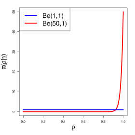
Figure 1: Two components of the spike and slab prior distribution for the $\rho$ parameters (the slab component is depicted in blue, and the spike one in red).

The prior on $\gamma$ is not the subject of this paper. It is typically used to control for multiplicity (Scott and Berger, 2010), an issue that, to the best of our knowledge, has not been addressed in the context of screening. Once the marginals have been computed, it is straightforward to include any prior on $\gamma$ via (7). In our numerical examples, the constant prior will be the implemented choice.

The prior on $\eta$ is broken down as $\pi(\mbox{\boldmath{$\eta$}})=\pi(\mbox{\boldmath{$\theta$}})\ \pi(\sigma^{2})\ \pi(\sigma_{0}^{2})$. Expert knowledge is usually utilized to specify $\pi(\mbox{\boldmath{$\theta$}})$. Inverse gamma distributions are chosen for the priors on the variances; see sections 4 and 5 for examples on how to specify the parameters of these priors. Then, we need an efficient way to compute the marginal $m(\mbox{\boldmath{$y$}}\mid\mbox{\boldmath{$\gamma$}})$ for all possible choices of $\gamma$.

3.2 Posterior inclusion probability computation

The ability to compute the marginal distribution of the observable under each of the competing models is one of the main computational obstacles to implementing model selection strategies. Han and Carlin (2001) offers a comparative review of most of the available tools to accomplish this task. Many are based on some post-processing of a sample from the posterior distribution of the model-specific parameters, and this means that one would need an MCMC sample from each of the competing models, which is not feasible even for relatively small $p$. Our problem has a very specific structure that can be exploited.

First, notice that the posterior distribution over the model space in (7) can be written as a function of the Bayes factors of each competing model to $\mathcal{M}_{\boldsymbol{1}}$:

$$B_{\boldsymbol{\gamma}}=\frac{m(\mbox{\boldmath{$y$}}\mid\mbox{\boldmath{$\gamma$}})}{m(\mbox{\boldmath{$y$}}\mid\mbox{\boldmath{$\gamma$}}=\mbox{\boldmath{$1$}})}$$ (13)

which is a ratio of normalizing constants. Since the support of the posterior is the same under model $\mathcal{M}_{\boldsymbol{\gamma}}$ and under model $\mathcal{M}_{\boldsymbol{1}}$, we can obtain (13) using a version of importance sampling (c.f., e.g., Chen and Shao, 1997) as an expectation with respect to the posterior under $\mathcal{M}_{\boldsymbol{1}}$

$$B_{\boldsymbol{\gamma}}=E_{\boldsymbol{1}}\left[\frac{f(\mbox{\boldmath{$y$}}\mid\mbox{\boldmath{$\rho$}},\mbox{\boldmath{$\eta$}},\mbox{\boldmath{$\gamma$}})\ \pi(\mbox{\boldmath{$\rho$}},\mbox{\boldmath{$\eta$}}\mid\mbox{\boldmath{$\gamma$}})}{f(\mbox{\boldmath{$y$}}\mid\mbox{\boldmath{$\rho$}},\mbox{\boldmath{$\eta$}},\mbox{\boldmath{$\gamma$}}=\mbox{\boldmath{$1$}})\ \pi(\mbox{\boldmath{$\rho$}},\mbox{\boldmath{$\eta$}}\mid\mbox{\boldmath{$\gamma$}}=\mbox{\boldmath{$1$}})}\right]\ ,$$ (14)

where $f(\mbox{\boldmath{$y$}}\mid\mbox{\boldmath{$\rho$}},\mbox{\boldmath{$\eta$}},\mbox{\boldmath{$\gamma$}})$ is given by (5). This allows us to estimate all the ratios using an MCMC sample from the full model only: if $\{\mbox{\boldmath{$\rho$}}^{(r)},\mbox{\boldmath{$\eta$}}^{(r)},\ r=1,\ldots,M\}$, is a sample from the posterior distribution of the unknowns for $\mbox{\boldmath{$\gamma$}}=\mbox{\boldmath{$1$}}$, then

$$\begin{split}B_{\boldsymbol{\gamma}}&\approx\frac{1}{M}\sum_{r=1}^{M}\ \frac{f(\mbox{\boldmath{$y$}}\mid\mbox{\boldmath{$\rho$}}^{(r)},\mbox{\boldmath{$\eta$}}^{(r)},\mbox{\boldmath{$\gamma$}})\ \pi(\mbox{\boldmath{$\rho$}}^{(r)},\mbox{\boldmath{$\eta$}}^{(r)}\mid\mbox{\boldmath{$\gamma$}})}{f(\mbox{\boldmath{$y$}}\mid\mbox{\boldmath{$\rho$}}^{(r)},\mbox{\boldmath{$\eta$}}^{(r)},\mbox{\boldmath{$\gamma$}}=\mbox{\boldmath{$1$}})\ \pi(\mbox{\boldmath{$\rho$}}^{(r)},\mbox{\boldmath{$\eta$}}^{(r)}\mid\mbox{\boldmath{$\gamma$}}=\mbox{\boldmath{$1$}})}\\ &=\frac{1}{M}\sum_{r=1}^{M}\ \pi(\mbox{\boldmath{$\rho$}}^{(r)}\mid\mbox{\boldmath{$\gamma$}})\end{split}$$ (15)

which is a consequence of (5) being the same regardless of $\gamma$, of the prior independence between $\rho$ and $\eta$ given $\gamma$, and of the fact that under the full model the prior on $\rho$ is a product of uniform distributions on the unit interval.

Note that this strategy would also potentially work in the linear regression context, because one would have to compute the ratio of normal densities centered at zero but with different variances, the one in the numerator having a much larger variance than the one on the denominator, which is not likely to be numerically unstable even for values far away from the origin. This will be explored elsewhere.

Once all $2^{p}-1$ Bayes factors are computed, it is straightforward to pair them with a prior on $\gamma$, e.g. the constant prior, and to obtain the posterior probabilities of each of the competing models. It then provides us with the so-called posterior (marginal) inclusion probabilities of each input

$$\pi(x_{\ell}\mid\mbox{\boldmath{$y$}})=\sum_{\boldsymbol{\gamma}:\ \gamma_{\ell}=1}\ \pi(\boldsymbol{\gamma}\mid\mbox{\boldmath{$y$}})$$ (16)

which are an easy to interpret measure of the importance of $x_{\ell}$ in explaining the response. Our approach to screening then reduces to the computation of such quantities and this is the reason for its acronym PIPS: posterior inclusion probability screening.

We can additionally obtain other interesting summaries, e.g. the posterior inclusion probability of a pair of variables:

$$\pi(x_{\ell}\vee x_{j}\mid\mbox{\boldmath{$y$}})=\pi(x_{\ell}\mid\mbox{\boldmath{$y$}})+\pi(x_{j}\mid\mbox{\boldmath{$y$}})-\sum_{\boldsymbol{\gamma}:\,\gamma_{\ell}=1,\gamma_{j}=1}\ \pi(\boldsymbol{\gamma}\mid\mbox{\boldmath{$y$}})$$ (17)

3.3 Slow computer code

When the computer model is slow, MCMC algorithms are typically unfeasible since they require many evaluations of the computer model. A classical technique is to bypass the computational effort by using a surrogate which approximates the computer model but is fast to run. Thus the surrogate can be plugged in the likelihood derived from the model given in (5) instead of the computer model. However, the main limitation of this approach lies in the fact that the bias not only accounts for the modeling error of the computer model but also for the discrepancy between the surrogate and the computer model.

Some surrogates are emulators, perhaps the most utilized being the GaSP emulator (Sacks et al., 1989; Currin et al., 1991). In addition to the fast approximation, they provide the practitioner with a measure of the additional source of uncertainty coming from the approximation. It is based on a limited number of runs of the computer model. We denote by $f(\mbox{\boldmath{$D$}})$ the corresponding outputs of the computer model with respect to the design of numerical experiments $\mbox{\boldmath{$D$}}=\{(\mbox{\boldmath{$x$}}^{*}_{i},\theta_{i}),i=1\ldots n_{D}\}$ which consists of combinations of configurations of input variables and model parameters. Note that the chosen values for the input variables $\mbox{\boldmath{$x$}}_{i}^{*}$ $(1\leq i\leq n_{D})$ are not necessary constrained to be chosen among the ones corresponding to the field data $\mbox{\boldmath{$x$}}_{i}$ $(1\leq i\leq n)$. In this approach, the computer model $f$ is then modeled as a GaSP. Usually, the principle of modularization (Liu et al., 2009) is used. The parameters of this GaSP are estimated using only the data $f(\mbox{\boldmath{$D$}})$ (and not the field data, $y$). The emulator then consists of the process conditioned on $f(\mbox{\boldmath{$D$}})$ with plugged-in parameters. It is still a Gaussian process, the conditional mean of which, denoted by $e(\cdot)$, gives an approximation of the computer model and the conditional covariance of which, denoted by $k(\cdot,\cdot)$, provides a measure on the uncertainty coming from this approximation. This source of uncertainty can be incorporated within the likelihood/statistical model:

$$\mbox{\boldmath{$y$}}\mid\mbox{\boldmath{$\psi$}},\sigma^{2},\sigma_{0}^{2},\mbox{\boldmath{$\theta$}},f(\mbox{\boldmath{$D$}})\sim N_{n}(\mbox{\boldmath{$e$}}(\mbox{\boldmath{$\theta$}}),\sigma_{f}^{2}\mbox{\boldmath{$K$}}+\sigma^{2}\mbox{\boldmath{$R$}}+\sigma_{0}^{2}\ \mbox{\boldmath{$I$}}_{n})$$ (18)

where $R$ and $\mbox{\boldmath{$I$}}_{n}$ are defined above, $\mbox{\boldmath{$e$}}(\mbox{\boldmath{$\theta$}})=(e(\mbox{\boldmath{$x$}}_{i},\mbox{\boldmath{$\theta$}}),\ i=1,\ldots,n)^{\top}$ are evaluations of the conditional mean of the emulator and $K$ is the $n\times n$ correlation matrix corresponding to the emulator, with entries $\mbox{\boldmath{$K$}}=[k((\mbox{\boldmath{$x$}}_{i},\theta),(\mbox{\boldmath{$x$}}_{j},\theta))]_{i,j=1,\ldots,n}$.

This will lead to a added computational burden in the MCMC algorithms, since now we have an additional correlation matrix $K$ that needs to be recomputed for each proposal of $\boldsymbol{\theta}$. However, there is no additional technical or conceptual difficulty to apply the PIPS method in the context of a slow computer model.

4 Simulation studies

The aim of this section is to assess the performance of the PIPS methodology in simulated scenarios. In §4.1, we compare the PIPS results with the results obtained using the RDVS method when screening the discrepancy function for active inputs. In §4.2, we introduce a simulation study where we try to mimic situations one might encounter when confronting field observations with the output of a computer model. All the computer codes utilized in the analyses of this section are available as an R package in https://github.com/Demiperimetre/PIPScreening.

4.1 Comparison between RDVS and PIPS

We consider a scenario where we have $p=8$ input variables. The $n=50$ experimental units will be chosen as a Latin-Hypercube-Design (LHD) and denoted as $\mbox{\boldmath{$x$}}_{i}=(x_{1i},x_{2i,}\dots,x_{pi})^{\top}\in[0,1]^{p}$, for $i=1,\ldots,n$.

The field observations will be generated from the model

$$y_{i}=f(\mbox{\boldmath{$x$}}_{i},\boldsymbol{\theta})+\delta(\mbox{\boldmath{$x$}}_{i})+\varepsilon_{i}$$

where

$$f(\mbox{\boldmath{$x$}}_{i},\boldsymbol{\theta})=\sum_{\ell=1}^{4}\frac{|4x_{\ell i}-2|+\theta_{\ell}}{1+\theta_{\ell}}\ .$$

The four parameters $(\theta_{j}$, $j=1,\ldots,k=4)^{\top}$ are fixed at $(0.3,0.4,0.5,0.6)^{\top}$. In the statistical analyses that will follow, these parameters will be considered either known and fixed at their true value, or as unknown, and in this case they will be calibrated.

The expression for the discrepancy function is

$$\delta(\mbox{\boldmath{$x$}}_{i})=\sin(2\pi x_{1i}\cdot x_{5i})+x_{2i}^{3}+(1-x_{6i})^{3}\ ,$$ (19)

which crucially depends only on $4$ of the $8$ original input variables, namely on $x_{1}$, $x_{2}$, $x_{5}$ and $x_{6}$. Finally, the measurement error was simulated as $\varepsilon_{i}\sim\mathcal{N}(0,\sigma_{0}^{2}=0.05^{2})$.

Notice that in this scenario we have variables which are both in the model and in the discrepancy function ($x_{1}$ and $x_{2}$), variables which only appear in the model ($x_{3}$ and $x_{4}$), variables which are only part of the discrepancy function ($x_{5}$ and $x_{6}$) and, finally, variables which do not appear neither in the model not in the discrepancy function ($x_{7}$ and $x_{8}$).

We used the model above to generate $100$ datasets. We then applied the proposed PIPS approach as well as the RDVS method to identify the variables which are active in the discrepancy function. As mentioned, we consider $\boldsymbol{\theta}$ to be fixed at its true value or unknown and hence calibrated. Notice that the discrepancy function is treated as unknown (i.e., the formula (19) used to generate the data is not used in the analysis) and is modeled as a GaSP as in (2). The measurement error variance $\sigma_{0}^{2}$ is also treated as unknown.

For the two methods, the MCMC algorithm consists in a combination of a Metropolis within Gibbs (MwG) algorithm followed by a Metropolis-Hastings (MH) algorithm. First, $5,000$ iterations of an MwG algorithm are run. Then, the covariance matrix of the posterior distribution of the parameters is estimated from this sample and is used in order to set the covariance of the proposal distribution of an MH algorithm. This MH algorithm is run for $10,000$ iterations. The proposal distributions are Gaussian random walks in 1 dimension for the MwG and in all dimensions for the MH algorithm. The parameters are transformed to lie in a non-constrained real interval. The variance parameters are then taken in the logarithm scale and the logit function is used to map the the model parameters to calibrate and the $\rho$ parameters (all lying in the unit interval) to the real interval.

For the PIPS method, this algorithm is run only once, while it is repeated $T=100$ times for the RDVS method, in order to learn the distribution of the posterior median for an inert input variable.

We fix the parameter $a$ in (6) at $a=1.9$. Regarding the prior distributions, both methods require a prior for the variances, which we specify as inverse gamma: $\sigma^{2}\sim\mathcal{IG}(3,1)$ and $\sigma^{2}_{0}\sim\mathcal{IG}(4,0.02)$. This implies that, a priori, we expect the variance of the discrepancy term to be larger than the measurement error variance. When the parameter $\theta$ is treated as unknown, a uniform distribution in the interval $[0,1]$ is set independently for each of its dimensions. The parameters in $\rho$ have all the slab part of the prior distribution since the MCMC algorithm is run only under the model $\mathcal{M}_{\boldsymbol{1}}$. For the RDVS method, we also used this prior distribution.

Regarding the post-processing of the posterior distribution that takes place in PIPS, we need to specify the spike part of the prior on $\rho_{\ell}$., Since the input variables are scaled to the $[0,1]$ interval, we set the shape parameters to be the same regardless of $\ell$: $\alpha_{\ell}=\alpha$. We have experimented with values for $\alpha$ ranging between $50$ and $200$, and have concluded that the computed posterior inclusion probabilities were not sensitive to the choice of $\alpha$ in this particular range. Accordingly, hereafter we fix this hyperparameter at $\alpha=100$.

For the RDVS method, the posterior median of the range parameter corresponding to each input variable is compared to a quantile of the posterior median of the range parameter of the fictitious variable. In particular, the three percentiles used are $5\%$, $10\%$ and $15\%$. Notice that Linkletter et al. (2006) argue for using a relatively large percentile in order to avoid missing an active variable; accordingly, they recommend the 10th percentile.

For the PIPS method, the posterior probability of activeness is compared to a threshold. The natural threshold is $0.5$ but, if one wants to be more conservative, one can choose a smaller one. In particular, we consider $0.1$, $0.5$ and $0.9$ and found the results to be not particularly sensitive to this choice in this example.

Tables 1 and 2 display the proportions of simulations where the variables are identified as active according to the two methods in competition under different settings. Table 1 corresponds to the case where the parameter $\boldsymbol{\theta}$ in the computer model is fixed at its true value, and Table 2 corresponds to the case where this parameter is simultaneously calibrated.

		$x_{1}$	$x_{2}$	$x_{3}$	$x_{4}$	$x_{5}$	$x_{6}$	$x_{7}$	$x_{8}$
RDVS	q5%	1.00	1.00	0.10	0.03	1.00	1.00	0.05	0.00
	q10%	1.00	1.00	0.15	0.05	1.00	1.00	0.07	0.00
	q15%	1.00	1.00	0.18	0.05	1.00	1.00	0.07	0.00
PIPS	th0.1	1.00	1.00	0.00	0.00	1.00	1.00	0.00	0.00
	th0.5	1.00	1.00	0.00	0.00	1.00	1.00	0.00	0.00
	th0.9	1.00	1.00	0.00	0.00	1.00	1.00	0.00	0.00

Table 1: Proportion of detection for a variable to be active when using RDVS and PIPS methods when the parameters $\boldsymbol{\theta}$ are fixed to their true values. For RDVS, the posterior median is compared with quantiles $q=5\%,10\%,15\%$ of the posterior median of the fictitious variable. For PIPS, the tested thresholds are fixed to $th=0.1,0.5,0.9$. Shadowed columns represent the truly active variables in the discrepancy function.

		$x_{1}$	$x_{2}$	$x_{3}$	$x_{4}$	$x_{5}$	$x_{6}$	$x_{7}$	$x_{8}$
RDVS	q5%	1.00	1.00	0.03	0.03	1.00	1.00	0.03	0.00
	q10%	1.00	1.00	0.07	0.05	1.00	1.00	0.03	0.00
	q15%	1.00	1.00	0.12	0.05	1.00	1.00	0.03	0.00
PIPS	th0.1	1.00	1.00	0.00	0.00	1.00	1.00	0.00	0.00
	th0.5	1.00	1.00	0.00	0.00	1.00	1.00	0.00	0.00
	th0.9	1.00	0.98	0.00	0.00	1.00	1.00	0.00	0.00

Table 2: Proportion of detection for a variable to be active when using RDVS and PIPS methods when the parameters $\boldsymbol{\theta}$ are calibrated. For RDVS, the posterior median is compared with quantiles $q=5\%,10\%,15\%$ of the posterior median of the fictitious variable. For PIPS, the tested thresholds are fixed to $th=0.1,0.5,0.9$. Shadowed columns represent the truly active variables in the discrepancy function

Both methods show convincing results regardless of whether the calibration was performed or not. The RDVS method may suffer from some false detection of active variables which increases as the quantile increases, as it may be expected. Hence, the PIPS method leads to results at least as good as the RDVS method but only requires one MCMC sample instead of a hundred. Furthermore, the PIPS method is stable and does not appear to be too sensitive to the choice of the threshold.

4.2 Idealized Scenarios of computer model validation

In the previous subsection, the goal was to establish the ability of PIPS to screen the discrepancy function for active inputs when compared with an alternative approach. For that reason, the setup of the experiment was arguably far too removed from a realistic situation, in that there was only uncertainty in the discrepancy function: the statistical analysis incorporated the knowledge of the analytic expression of the computer model that was actually used to generate the field data. In this subsection, we make an effort to construct more realistic scenarios. We want to mimic plausible situations that one might encounter when analyzing a computer model and flesh out the advantages brought by PIPS in the realm of uncertainty quantification. These simulations can be replicated from the vignette available at https://demiperimetre.github.io/PIPScreening/articles/ExampleScenario.html.

With this purpose in mind, we used the values of 100 observations on 5 input variables $\mbox{\boldmath{$x$}}^{\top}=(x_{1},x_{2},x_{3},x_{4},x_{5})\in[0,1]^{5}$ all simulated from independent uniform distributions except for $x_{3}$ and $x_{5}$, which are correlated.

Then, we simulated the field data according to

$$y_{i}=\zeta(\mbox{\boldmath{$x$}}_{i},\boldsymbol{\theta})+\epsilon_{i},\quad i=1,\ldots,100,$$

with $\zeta(\mbox{\boldmath{$x$}}_{i},\boldsymbol{\theta})$ differing in each scenario and $\varepsilon_{i}\sim\mathcal{N}(0,\sigma_{0}^{2}=0.05^{2})$. Conceptually, $\zeta(\mbox{\boldmath{$x$}}_{i},\boldsymbol{\theta})$ is the reality which the computer model is built to replicate.

The statistical analysis of the data is constructed under the assumption that the actual computer model is

$$f(\mbox{\boldmath{$x$}}_{i},\boldsymbol{\theta})=\sum_{\ell=1}^{3}\frac{|4x_{\ell i}-2|+\theta_{\ell}}{1+\theta_{\ell}}\,$$

where $\boldsymbol{\theta}$ may either be known or calibrated. We also consider a discrepancy function $\delta(\mbox{\boldmath{$x$}}_{i})$, which is a function of all 5 variables, meant to capture the differences between reality and the computer model. Notice that the computer model only involves the first 3 input variables.

In particular, the considered four different situations:

1. $x_{1}$ is incorrectly modeled by the computer model:

   $$\zeta(\mbox{\boldmath{$x$}}_{i},\boldsymbol{\theta})=\frac{|4x_{1i}^{2}-2|+\theta_{1}}{1+\theta_{1}}+\frac{|4x_{2i}-2|+\theta_{2}}{1+\theta_{2}}+\frac{|4x_{3i}-2|+\theta_{3}}{1+\theta_{3}},$$

2. $x_{2}$ has no impact in reality:

   $$\zeta(\mbox{\boldmath{$x$}}_{i},\boldsymbol{\theta})=\frac{|4x_{1i}-2|+\theta_{1}}{1+\theta_{1}}+\frac{|4x_{3i}-2|+\theta_{3}}{1+\theta_{3}},$$

3. $x_{4}$ was forgotten in the computer model:

   $$\zeta(\mbox{\boldmath{$x$}}_{i},\boldsymbol{\theta})=\frac{|4x_{1i}-2|+\theta_{1}}{1+\theta_{1}}+\frac{|4x_{2i}-2|+\theta_{2}}{1+\theta_{2}}+\frac{|4x_{3i}-2|+\theta_{3}}{1+\theta_{3}}+\frac{|4x_{4i}-2|+\theta_{4}}{1+\theta_{4}},$$

4. $x_{3}$ instead of $x_{5}$ is in the computer model

   $$\zeta(\mbox{\boldmath{$x$}}_{i},\boldsymbol{\theta})=\frac{|4x_{1i}-2|+\theta_{1}}{1+\theta_{1}}+\frac{|4x_{2i}-2|+\theta_{2}}{1+\theta_{2}}+\frac{|4x_{5i}-2|+\theta_{5}}{1+\theta_{5}}.$$

From these four situations, we build three scenarios, which are combinations of Case 1 ($x_{1}$ is squared in the physical reality while it is linear in the computer model) with the three other cases. The vector of model parameters is chosen as $(\theta_{1},\theta_{2},\theta_{3},\theta_{4},\theta_{5})^{\top}=(0.4,0.5,0.6,0.7,0.8)^{\top}$.

MCMC and prior specifications were exactly as laid out in the previous subsection, including setting $a=1.9$ in (6) and $\alpha_{\ell}=\alpha=100$.

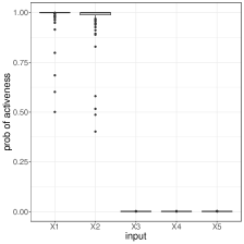
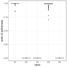
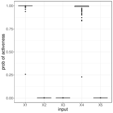
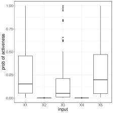
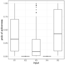
Figure 2: Boxplots of the probabilities of activeness over the $100$ replications. On the left are the cases with parameters fixed to their true values and, on the right, the case where the parameters are considered unknown and calibrated. From top to bottom, mixed of cases 1 and 2, mixed of cases 1 and 3, and mixed of cases 1 and 4.

Figure 2 provides the boxplots of the probabilities of activeness of the input variables in the discrepancy function under the different scenarios. For the two first cases, the results are clear and the variables which differ from the computer model to reality appear as active variables in the discrepancy function. For the last case, which is more difficult because an active variable is not in the computer model but another one correlated with it is, the PIPS method manages to detect that something is happening with these input variables, although the probabilities of activeness stay mostly under the $0.5$ threshold.

5 A photovoltaic plant computer model

In this section, we introduce a real application which was studied by Carmassi et al. (2019). The idea is to use a computer model to predict the power produced by a photovoltaic plant (PVP) given some meteorological conditions such as the temperature and the sun irradiation. The computer model also depends on some parameters which can be fixed at so-called nominal values specified using expert knowledge or can be calibrated from experimental data.

Here, we will use the experimental data in order to learn about possible model misspecification by screening the discrepancy function using the PIPS methodology.

The computer model aims at mimicking the behavior of a PVP consisting of 12 panels connected together. This computer model is quick to run and can be represented by a function $f:\mathbb{R}^{4}\times\mathbb{R}^{6}\owns(\mbox{\boldmath{$x$}},\boldsymbol{\theta})\mapsto y\in\mathbb{R}$. The input variables $\mbox{\boldmath{$x$}}=(t,I_{g},Id,T_{e})^{\top}$ consist of $t$, the UTC time since the beginning of the year, $I_{g}$, the global irradiation of the sun, $I_{d}$ the diffuse irradiation of the sun, and $T_{e}$, the ambient temperature. The parameter $\boldsymbol{\theta}$ consists actually of $6$ parameters but only one parameter is calibrated, the module photo-conversion efficiency. A sensitivity analysis has proven the other parameters to be of negligible importance. The output $y$ is the resulting instantaneous power delivered by the PVP.

The experimental data correspond to the test stand of 12 panels and were collected over two months every $10$ seconds, which makes for a huge amount of data. Only the data for which the production is positive are kept, corresponding to daytime measurements. The data contain the power production, which is to be compared with the output of the computer model; the four input variables of the computer model and an additional temperature (temperature on the panel, $T_{p}$) were also recorded. Although this last variable is not an input variable of the computer model, it is tested as a potential active variable in the discrepancy.

5.1 Detecting active variables in the discrepancy

In order to detect the input variables which may cause the discrepancy between the computer model output and the reality, we applied the PIPS methodology to the data obtained on a single day. The considered days are in August and September 2014. September 7 was removed since the recorded production was null which is a consequence of a sensor malfunction.

To limit the computational burden for a given day, we took a measurement every five minutes, which gives between 99 and 178 data points per day. Figure 3 illustrates four different days of power recording. Although these four days exhibit somewhat different patterns of production, the common feature is the global increase in production beginning at sun rise followed by a decay which reaches a null production when the sun sets. Higher frequency peaks may be a consequence of clouds limiting the sun irradiation. We emphasize that this case study is challenging because of the structure of the correlation between the input variables in the computer model.

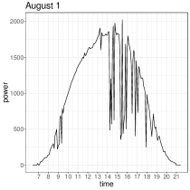
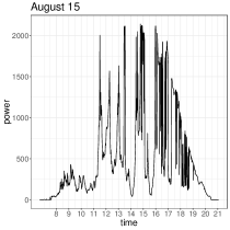
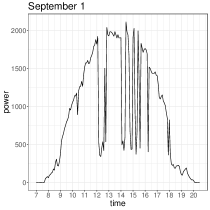
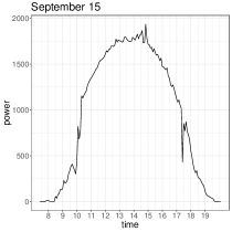
Figure 3: Power produced by the PV power plant on days: August 1st, August 15, September 1st, September 15. A measure every five minutes is kept for a positive production.

We consider the situation where all the parameters were fixed at their nominal value and when the module photo-conversion efficiency is calibrated simultaneously with the detection of active variables. All the input variables and the model parameter were scaled to the $[0,1]$ interval. The output data were normalized by subtracting their mean and divided by their standard deviation. The prior distributions for the variances of the measurement error and the discrepancy were chosen as inverse gamma distribution with parameters favoring a larger variance for the discrepancy and in line with the known precision of sensors, namely, $\mathcal{IG}(4,1/400)$ for the measurement error and $\mathcal{IG}(2,1/200)$ for the variance corresponding to the GaSP which models the discrepancy. A uniform prior within an interval provided by experts was used for the only parameter to calibrate. We also choose $a=1.9$ in the correlation kernel defined in (6), and set $\alpha_{\ell}=\alpha=100$.

The MCMC set up is the same as the one used in the examples presented in Section 4. Using the resulting sample, we obtain the posterior probabilities of activeness for each day as well as the probability that at least one of the two temperatures ($T_{e}$ and $T_{p}$) is active in the discrepancy.

Figure 4 provides the boxplots of these probabilities computed for 60 days of data, that is, the boxplots describe the set of 60 activeness probabilities corresponding to each of the days. For the two first variables (time $t$ and global irradiation $I_{g}$) the results are clearly in favor of including them in the discrepancy. For the diffuse irradiation $I_{d}$ and the two temperatures the results are less clear. Still, the results show that at least one of the two temperatures should be included in the discrepancy and it seems that the ambient temperature $T_{e}$ is a little bit more important. When the computer model is calibrated simultaneously, the calibrated value is shifted toward its upper bound (more than $75\%$ of the days).

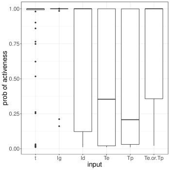
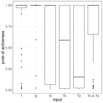
Figure 4: Boxplots of probabilities of activeness of the input variables in the discrepancy computed for the 60 days of data. The column $(T_{e}\textrm{ or }T_{p})$ corresponds to the fact that at least one of two temperatures is active. The top boxplots correspond to the case when the parameter $\theta$ is fixed to its nominal value. The bottom boxplots correspond to the case when $\theta$ is calibrated.

Related analysis of these data

In Carmassi et al. (2019), the computer model was calibrated by assuming different statistical models with or without the discrepancy function. When the discrepancy function was part of the model, an isotropic Gaussian kernel was chosen. The temperature on the panel was not considered in the discrepancy. Only the four input variables of the computer model were taken into account in the discrepancy, which makes for a 4-dimensional input space. In addition, to limit the size of the data, they made the choice to compute hourly averages of the input variables and of the power produced. The discrepancy was found to play an important role. We tried the same strategy by only keeping the hours after 8 a.m. and before 7 p.m. where the production is likely to be higher. It resulted in $572$ hourly measurements. When screening the discrepancy, all the variables were found active. This is quite expected since the computer model is not directly run on the observed input data but on averages of these input data.

6 Conclusion

In this paper, we focused on screening the discrepancy function which is used to model the gap between a real phenomenon and its “in silico” simulation. The outcome of the screening procedure should help provide the practitioner with a better understanding of the flaws of the computer model by determining which input variables are incorrectly taken into account, i.e., the ones that are active in the discrepancy function. We cast this screening procedure into the more general problem of variable selection for GaSP regression. We then proposed an original method, named PIPS, which aims to select the active variables on the basis of a unique MCMC sample. The efficiency of the PIPS method was demonstrated on synthetic examples and was also illustrated on a real world application. Although the computer model in the applications were fast enough so that we did not need to resort to an emulation step, the PIPS method could be combined with an emulator. However, one has to be careful that, in this case, the discrepancy may account for both the flaws of the computer model and of its emulator.

The PIPS method relies on the enumeration of $2^{p}$ models, which might may be unfeasible if $p$ is too large (say $p>20$). In this case, the strategies described in Garcia-Donato and Martinez-Beneito (2013) should obtain reliable estimates of the posterior inclusion probabilities for moderately large values of $p$.

A particular concern is the performance of the MCMC sampling, which is crucial. Adaptive MCMC schemes could be combined with some intermediate results from the PIPS method in order to reinforce the sampling in the dimensions where the input variables are the most likely to be active. A complementary issue is the determination of the validity area of the computer model. The PIPS method could then be used to feed adaptive design strategies to accurately determine this region.

Appendix A Proof of the theorem

Conditions on the prior distribution

We assume that the prior distribution $\pi(\mbox{\boldmath{$\eta$}})=\pi(\mbox{\boldmath{$\theta$}},\sigma^{2},\sigma_{0}^{2})$ has a compact support that does not contain points such that $\sigma^{2}=0$ or $\sigma_{0}^{2}=0$. Moreover, we assume this prior to be proper and bounded.

Proof

Without loss of generality, let us assume that $\ell=1$. We consider the sequence of prior distribution $\pi^{n}(\rho_{1})=n\rho_{1}^{n-1}$, $0<\rho_{1}<1$ which corresponds to the $\mathcal{B}(n,1)$ distribution. Let $\mbox{\boldmath{$\eta$}}=(\sigma^{2},\sigma_{0}^{2},\mbox{\boldmath{$\theta$}})^{\top}$ and $\mbox{\boldmath{$\rho$}}_{(-1)}=(\rho_{2},\ldots,\rho_{p})^{\top}$. Additionally, denote by $g(\boldsymbol{y}\mid\boldsymbol{\rho},\boldsymbol{\eta})$ the density of the field data corresponding to the sampling distribution given in (5).

First step: we prove that, as a consequence of the dominated convergence theorem,

$$\lim_{n\rightarrow\infty}\int_{\boldsymbol{\eta},\boldsymbol{\rho}_{(-1)}}\int_{\rho_{1}}g(\boldsymbol{y}\mid\boldsymbol{\rho},\boldsymbol{\eta})\ \pi(\boldsymbol{\rho}\mid\mbox{\boldmath{$\gamma$}})\ \pi(\boldsymbol{\eta})\ d\rho_{1}\ d\boldsymbol{\eta}\ d\boldsymbol{\rho}_{(-1)}$$

$$=\int_{\boldsymbol{\eta},\boldsymbol{\rho}_{(-1)}}\left(\lim_{n\rightarrow\infty}\int_{\rho_{1}}g(\boldsymbol{y}\mid\boldsymbol{\rho},\boldsymbol{\eta})\ \pi^{n}(\rho_{1})\ d\rho_{1}\right)\pi(\boldsymbol{\rho}_{(-1)})\ \pi(\boldsymbol{\eta})\ d\boldsymbol{\eta}\ d\boldsymbol{\rho}_{(-1)}\ .$$

The dominated convergence theorem applies, since for all $n$, we have

$$\int_{\rho_{1}}g(\boldsymbol{y}\mid\boldsymbol{\rho},\boldsymbol{\eta})\ \pi^{n}(\rho_{1})\ d\rho_{1}\leq\sup_{\boldsymbol{\rho},\boldsymbol{\eta}}g(\boldsymbol{y}\mid\boldsymbol{\rho},\boldsymbol{\eta})\int\pi^{n}(\rho_{1})\ d\rho_{1}=\sup_{\boldsymbol{\rho},\boldsymbol{\eta}}\ g(\boldsymbol{y}\mid\boldsymbol{\rho},\boldsymbol{\eta})\cdot 1<+\infty\,.$$

Indeed, the inequality above ensures that the function

$$\boldsymbol{\rho}_{(-1)},\boldsymbol{\eta}\mapsto\int_{\rho_{1}}g(\boldsymbol{y}\mid\boldsymbol{\rho},\boldsymbol{\eta})\ \pi^{n}(\rho_{1})\ d\rho_{1}\ \pi(\boldsymbol{\rho}_{(-1)})\ \pi(\boldsymbol{\eta})$$

is bounded, for all $n$, by $\sup_{\boldsymbol{\rho},\boldsymbol{\eta}}g(\boldsymbol{y}\mid\boldsymbol{\rho},\boldsymbol{\eta})\ \pi(\boldsymbol{\rho}_{(-1)})\ \pi(\boldsymbol{\eta})$ which is integrable provided that the supremum is finite. The supremum is taken over the compact set corresponding to the compact support of the prior distribution of $\boldsymbol{\eta}$ and $\boldsymbol{\rho}$. This supremum is finite since the priors are bounded and $\sup_{\boldsymbol{\rho},\boldsymbol{\eta}}g(\boldsymbol{y}\mid\boldsymbol{\rho},\boldsymbol{\eta})$ is the supremum of the image of a compact set by a continuous function (a Gaussian likelihood as a function of its parameters where there are no singularities because the compact domain does not contain configurations of parameters such that $\sigma^{2}=0$ or $\sigma_{0}^{2}=0$). Therefore, the dominated convergence theorem applies.

Second step: By using integration by parts, we have

$$\int_{\rho_{1}}g(\boldsymbol{y}\mid\boldsymbol{\rho},\boldsymbol{\eta})\ \pi^{n}(\rho_{1})d\rho_{1}=\int_{\rho_{1}}g(\boldsymbol{y}\mid\boldsymbol{\rho},\boldsymbol{\eta})\ n\rho_{1}^{n-1}d\rho_{1}$$

$$=\left[g(\boldsymbol{y}\mid\boldsymbol{\rho},\boldsymbol{\eta})\right]_{\rho_{1}=0}^{\rho_{1}=1}-\int\frac{\partial}{\partial\rho_{1}}\ g(\boldsymbol{y}\mid\boldsymbol{\rho},\boldsymbol{\eta})\ \rho_{1}^{n}d\rho_{1}$$

$$=g(\boldsymbol{y}\mid(1,\boldsymbol{\rho}_{(-1)}),\boldsymbol{\eta})\cdot 1-g(\boldsymbol{y}\mid(0,\boldsymbol{\rho}_{(-1)})),\boldsymbol{\eta})\cdot 0-\int\frac{\partial}{\partial\rho_{1}}g(\boldsymbol{y}\mid\boldsymbol{\rho},\boldsymbol{\eta})\ \rho_{1}^{n}\ d\rho_{1}\ .$$

Third step: by showing that $\int\frac{\partial}{\partial\rho_{1}}\ g(\boldsymbol{y}\mid\boldsymbol{\rho},\boldsymbol{\eta})\ \rho_{1}^{n}\ d\rho_{1}\rightarrow 0$ as $n\rightarrow\infty$, the proof will be complete.

We apply again the dominated convergence theorem. For $n_{0}$ large enough, we have:

$$\left|\frac{\partial}{\partial\rho_{1}}g(\boldsymbol{y}\mid\boldsymbol{\rho},\boldsymbol{\eta})\ \rho_{1}^{n}\right|\leq\left|\frac{\partial}{\partial\rho_{1}}g(\boldsymbol{y}\mid\boldsymbol{\rho},\boldsymbol{\eta})\ \rho_{1}^{n_{0}}\right|\,.$$

The function $\rho_{1}\mapsto\frac{\partial}{\partial\rho_{1}}\ g(\boldsymbol{y}\mid\boldsymbol{\rho},\boldsymbol{\eta})$ is continuous in $[0,1]$ and $C^{\infty}$ in $(0,1]$ because of the form of the covariance function and the polynomial expression of the inverse and the determinant functions in the likelihood. We can extend by continuity to $0$ the function $\rho_{1}\mapsto\frac{\partial}{\partial\rho_{1}}\ g(\boldsymbol{y}\mid\boldsymbol{\rho},\boldsymbol{\eta})\ \rho_{1}^{n_{0}}$, the evaluation of which will be $0$ since the derivative of the likelihood is polynomial in $1/\rho_{1}$. For this reason, $n_{0}$ needs to be chosen large enough to compensate.

References

- Bai et al. (2020) Bai, R., V. Rockova, and E. I. George (2020). Spike-and-slab meets lasso: a review of the spike-and-slab lasso. arXiv preprint arXiv:2010.06451.
- Bayarri et al. (2007a) Bayarri, M. J., J. O. Berger, R. Paulo, J. Sacks, J. A. Cafeo, J. Cavendish, C.-H. Lin, and J. Tu (2007a). A framework for validation of computer models. Technometrics 49(2), 138–154.
- Bayarri et al. (2007b) Bayarri, M. J., J. O. Berger, R. Paulo, J. Sacks, J. A. Cafeo, J. Cavendish, C.-H. Lin, and J. Tu (2007b). A framework for validation of computer models. Technometrics 49(2), 138–154.
- Brynjarsdóttir and O’Hagan (2014) Brynjarsdóttir, J. and A. O’Hagan (2014, oct). Learning about physical parameters: the importance of model discrepancy. Inverse Problems 30(11), 114007.
- Carmassi et al. (2019) Carmassi, M., P. Barbillon, M. Keller, Éric Parent, and M. Chiodetti (2019). Bayesian calibration of a numerical code for prediction. Journal de la Société Française de Statistique accepted.
- Chen and Shao (1997) Chen, M.-H. and Q.-M. Shao (1997). On monte carlo methods for estimating ratios of normalizing constants. Ann. Statist. 25(4), 1563–1594.
- Chen and Wang (2010) Chen, T. and B. Wang (2010). Bayesian variable selection for gaussian process regression: Application to chemometric calibration of spectrometers. Neurocomputing 73(13-15), 2718–2726.
- Clyde and George (2004) Clyde, M. and E. I. George (2004, 02). Model uncertainty. Statist. Sci. 19(1), 81–94.
- Craig et al. (2001) Craig, P. S., M. Goldstein, J. C. Rougier, and A. H. Seheult (2001). Bayesian forecasting for complex systems using computer simulators. Journal of the American Statistical Association 96(454), 717–729.
- Currin et al. (1991) Currin, C., T. Mitchell, M. Morris, and D. Ylvisaker (1991). Bayesian prediction of deterministic functions, with applications to the design and analysis of computer experiments. Journal of the American Statistical Association 86(416), 953–963.
- Damblin et al. (2016) Damblin, G., M. Keller, P. Barbillon, A. Pasanisi, and É. Parent (2016). Bayesian model selection for the validation of computer codes. Quality and Reliability Engineering International 32(6), 2043–2054.
- Garcia-Donato and Martinez-Beneito (2013) Garcia-Donato, G. and M. A. Martinez-Beneito (2013). On Sampling strategies in Bayesian variable selection problems with large model spaces. Journal of the American Statistical Association 108(501).
- George and McCulloch (1993) George, E. I. and R. E. McCulloch (1993). Variable selection via Gibbs sampling. Journal of the American Statistical Association 88(423), 881–889.
- Gramacy and Lee (2012) Gramacy, R. B. and H. K. H. Lee (2012). Cases for the nugget in modeling computer experiments. Statistics and Computing 22(3), 713–722.
- Gu and Wang (2018) Gu, M. and L. Wang (2018). Scaled Gaussian stochastic process for computer model calibration and prediction. SIAM/ASA Journal on Uncertainty Quantification 6(4), 1555–1583.
- Han and Carlin (2001) Han, C. and B. P. Carlin (2001). Markov chain monte carlo methods for computing bayes factors. Journal of the American Statistical Association 96(455), 1122–1132.
- Higdon et al. (2004) Higdon, D., M. Kennedy, J. C. Cavendish, J. A. Cafeo, and R. D. Ryne (2004). Combining field data and computer simulations for calibration and prediction. SIAM Journal on Scientific Computing 26(2), 448–466.
- Kamary et al. (2019) Kamary, K., M. Keller, P. Barbillon, C. Goeury, and Éric Parent (2019). Computer code validation via mixture model estimation.