Homeostatic Criticality in Neuronal Networks

Abstract

In self-organized criticality (SOC) models, as well as in standard phase transitions, criticality is only present for vanishing external fields $h\to 0$. Considering that this is rarely the case for natural systems, such a restriction poses a challenge to the explanatory power of these models. Besides that, in models of dissipative systems like earthquakes, forest fires, and neuronal networks, there is no true critical behavior, as expressed in clean power laws obeying finite-size scaling, but a scenario called “dirty” criticality or self-organized quasi-criticality (SOqC). Here, we propose simple homeostatic mechanisms which promote self-organization of coupling strengths, gains, and firing thresholds in neuronal networks. We show that with an adequate separation of the timescales for the coupling strength and firing threshold dynamics, near criticality (SOqC) can be reached and sustained even in the presence of significant external input. The firing thresholds adapt to and cancel the inputs ($h$ decreases towards zero). Similar mechanisms can be proposed for the couplings and local thresholds in spin systems and cellular automata, which could lead to applications in earthquake, forest fire, stellar flare, voting, and epidemic modeling.

Highlights

• We introduce a novel mechanism that promotes Self-organized quasicriticality (SOqC) even in the presence of external fields;

• Criticality is asymptotically approached as the ratio between the homeostatic time scales increases;

• The mechanism is general and can be applied to any phase transition.

I Introduction

The idea of self-organized criticality (SOC) [1], in which a given dynamical system has a critical point as an attractor, without any ad hoc imposition of parameter values (fine-tuning), in some sense has never truly been achieved. The most successful models under this ideal display bulk conservation, such as in the Abelian sandpile [2, 3, 4]. However, this conservation requirement can also be seen as a form of fine-tuning, since the number of dissipated grains in the spread of avalanches must be zero. Moreover, the infinite separation of time scales between driving and avalanches in SOC models can be viewed as yet another form of fine-tuning.

When we consider dissipative systems such as earthquakes, forest fires or neural networks, we find that only self-organized quasicriticality (SOqC) holds [5, 6]. This regime is characterized by the system performing stochastic oscillations around the critical point. Several of such models include continuous drive and dissipation, some of which can be viewed as homeostatic mechanisms that drive the network toward the critical point.

In the case of cortical models, SOqC mechanisms have been widely employed to explain the experimental observation of neuronal avalanches [7, 8, 9, 10, 11]. The main studied homeostatic mechanisms are related to synaptic dynamics [12, 13, 14], but dynamical gains [15, 16, 17, 18] and firing thresholds have also been considered [19, 20, 21] (for a review see [22]).

In the absence of homeostatic mechanisms, a critical regime is obtained only with strong and non-local fine-tuning over, for example, all coupling weights (synapses) $W_{ij}$, so that the distribution $P(W_{ij})$ must have average $\left\langle W_{ij}\right\rangle\equiv W=W_{c}$ (the control parameter). With homeostasis, this constraint is relaxed: now we can start from any distribution $P_{t=0}(W_{ij})$ and, after a transient (the self-organization process), one obtains a stationary $P^{*}(W_{ij})\equiv\lim_{t\rightarrow\infty}P(W_{ij})$ where $W^{*}\equiv\lim_{t\rightarrow\infty}\left\langle W_{ij}\right\rangle\approx W_{c}$. Similar reasoning applies to neuronal gains $\Gamma_{i}$ and firing thresholds $\theta_{i}$.

One important aspect in any SOC model is that phase transitions, and therefore criticality, exist only for zero or very small external field [4, 23, 24], so any homeostatic mechanism will need to self-organize the system to a state where the effective external field vanishes.

Here, we propose a solution to this problem by unveiling an interplay between homeostatic time scales, network size and external field. We show that the important factor behind the generation of power-law avalanches that obey the size-duration scaling law is sensory adaptation, mediated by dynamic firing thresholds. This adaptation must occur over long periods of time when compared to the intrinsic neuronal and synaptic time scales.

We develop a mean-field theory for the homeostatic model, and compare it to simulation results for a sparse random network with $K$ input neighbors per node. These mechanisms are simple and very general: they can be adapted to systems composed of other units such as spins, cellular automata, discrete time maps or continuous time neuronal models with pulse coupling given by weights $W_{ij}$.

II The model and its mean-field approximation

We consider a network of $N$ discrete-time stochastic leaky integrate-and-fire neurons [25, 26, 27, 15, 16, 18, 28]. A binary indicator $X_{i}\in\{0,1\},i=1,\ldots,N$, denotes silence ($X_{i}=0$) or the firing of an action potential (spike, $X_{i}=1$). The membrane potential of neuron $i$ evolves according to:

$$V_{i}(t+1)=\mu_{i}V_{i}(t)+I_{i}+\frac{1}{K}\sum_{j=1}^{N}W_{ij}X_{j}(t)\>,$$ (1)

where $0\leq\mu_{i}\leq 1$ are leakage parameters and $I_{i}$ are external inputs. The directed synaptic weight matrix $W_{ij}$ has exactly $K$ incoming links from $j$ to $i$. The outgoing links, by this construction, have a binomial distribution with average $K$ and standard deviation $\sigma=\sqrt{K(1-K/(N-1))}$. Notice that while the sum is over all $N$ potential neighbors (all $W_{ij}$ entries, most of them are zero for finite $K$), the normalization considers only the true $K$ (not $N$) neighbors. In the case of a complete graph, we use $K=N-1$ given that $W_{ii}=0$.

If a neuron fires at time step $t$, its membrane potential is reset, $V_{i}(t+1)=0$. Otherwise, its voltage is updated according to Eq. (1). A spike occurs with probability

$$P\left(X_{i}(t)=1\>|\>V_{i}(t)\right)\equiv\Phi(V_{i}(t))\>,$$ (2)

where $\Phi(V)$ is the so-called firing function. The model incorporates an absolute refractory period of one time step by imposing $\Phi(0)=0$. For this class of models, there are no strong requirements on the firing function $\Phi$ besides a sigmoidal shape. For analytical convenience, we adopt a linear-saturating shape [27, 15, 20, 21]:

$$\Phi(V_{i})=\begin{cases}0&\text{if }V_{i}<\theta_{i}\\ \Gamma_{i}\left(V_{i}-\theta_{i}\right)&\text{if }\theta_{i}<V_{i}<V_{i}^{S}\\ 1&\text{if }V_{i}>V_{i}^{S}\end{cases}$$ (3)

where $V_{i}^{S}=1/\Gamma_{i}+\theta_{i}$ is the saturation potential. Here, $\theta_{i}$ represents a firing threshold for neuron $i$. This choice of firing function implies that there is a finite probability of the $i$-th neuron emitting a spike only when $V_{i}(t)>\theta_{i}$, which increases linearly with $V_{i}$.

In the absence of homeostatic tuning (which we call the static model), assuming that the distribution $P(W_{ij})$ has finite variance, the average synaptic weight $W\equiv\left\langle W_{ij}\right\rangle$ can be taken as a control parameter. The same applies to the neuronal gains $\Gamma_{i}$, firing thresholds $\theta_{i}$, leakage parameters $\mu_{i}$ and inputs $I_{i}$, so that $\Gamma=\left\langle\Gamma_{i}\right\rangle$ and $\mu=\left\langle\mu_{i}\right\rangle$ can also be considered as control parameters. Interpreting $\theta=\left\langle\theta_{i}\right\rangle$ as the average local field (local adaptation current) and $I=\left\langle I_{i}\right\rangle$ as the average external field (external input current), we have that $h=I-\theta$ is the total or effective field.

The fraction of spiking neurons, also known as firing density or firing rate, $\rho(t)=\left\langle X_{i}(t)\right\rangle\equiv\frac{1}{N}\sum_{i=1}^{N}X_{i}(t)$ represents the activity of the network. The time average of $\rho(t)$ is calculated in the steady state and is the relevant order parameter. A summary of variables and parameters used in this work is presented in Table 1.

Table 1: Variables and parameters used in the model.

Variable	Symbol
Neuron state (binary)	$X_{i}$
Membrane potential	$V_{i}$
Saturation potential	${V_{i}}^{S}$
External field (input current)	$I_{i}$
Firing probability function	$\Phi$
Firing density (activity)	$\rho$
Effective external field	$h_{i}$
Neuronal gain	$\Gamma_{i}$
Synaptic weight	$W_{ij}$
Firing threshold	$\theta_{i}$

Parameter	Symbol
Number of input neighbors	$K$
Leakage parameter	$\mu_{i}$
Neuronal gain recovery time	$\tau_{\Gamma}$
Synaptic weight recovery time	$\tau_{W}$
Neuronal gain depression	$U_{\Gamma}$
Synaptic weight depression	$U_{W}$
Synaptic weight baseline	$A_{i}$
Neuronal gain baseline	$B_{i}$
Time scale ratio: threshold/synaptic	$a$
Depression ratio: threshold/synaptic	$b$

When $\Gamma$, $W$ and $\theta$ are fixed (static model), a mean-field approximation (equivalent to taking the $K\to\infty$ limit) can be calculated from:

$$\rho(t+1)=\int\Phi(V)P_{t}(V)\>dV\>,$$ (4)

where $P_{t}(V)$ is the distribution of voltages at time $t$  [15, 18].

For $\mu=0$, considering the case where the stationary potentials fall within the linear ($0<V_{i}<V_{i}^{S}$) branch of equation (3), the solution leads to the mean-field map:

$$\rho(t+1)=(1-\rho(t))\Gamma(W\rho(t)+h)\>\>.$$ (5)

The steady state is the fixed point of equation (5):

$$\rho^{\pm}=\frac{\Gamma W-1-\Gamma h\pm\sqrt{(\Gamma W-1-\Gamma h)^{2}+4\Gamma^{2}Wh}}{2\Gamma W}\>.$$ (6)

The phase transitions of this model are given by the bifurcations of the map in equation (5) [29]. When the field $h$ is negative, we have a discontinuous (first order) phase transition and, when $h>0$, there is always activity $\rho>0$ and no transition [15, 20].

For $h=0$, we have a second order phase transition, which is given by:

$$\rho(W,\Gamma)\sim\left(\frac{W-W_{c}(\Gamma)}{W_{c}(\Gamma)}\right)^{\beta}$$ (7)

for $W>W_{c}=1/\Gamma$, while $\rho=0$ (absorbing state) for $W<W_{c}$. The order parameter exponent is $\beta=1$. The hyperbola $W_{c}(\Gamma)=1/\Gamma$ is a critical line in the $W\times\Gamma$ plane. Similarly to what occurs in the Ising model, where the important variable is the combined quantity $J/T$, here the important variable is $\tilde{W}\equiv\Gamma W$, which defines the critical point $\tilde{W}_{c}=1$ (see Fig. 1). At $\tilde{W}=2$, a period-2 orbit is created. However, it is not relevant to the present work and has been studied in detail elsewhere [15, 20].

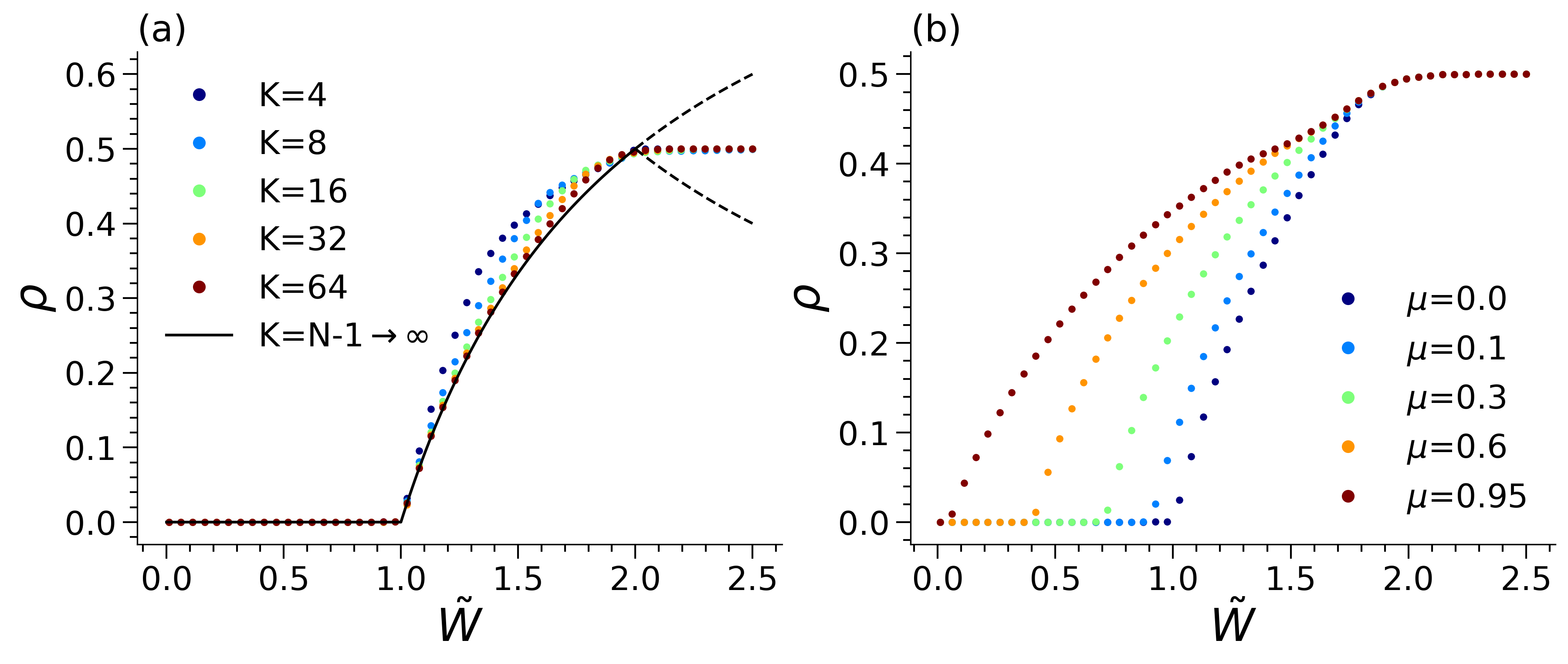
Figure 1: a) Order parameter $\rho(\tilde{W};\mu=0$) as a function of $\tilde{W}$ for different number of input neighbors $K$. From left to right, $K=4,8,16,32$ and mean-field (solid). The bifurcation at $\tilde{W}=2$ leads to the creation of a period$-2$ synchronous regular state [15, 20]. b) $\rho(\tilde{W};K=32)$ for various leakage parameters $\mu$. From right to left, $\mu=0,0.1,0.3,0.6$ and $0.95$. Network size $N=10^{4}$. The leakage parameter does not change the critical exponents, only shifts the critical point [21].

For random networks, a continuous phase transition is also observed:

$$\rho(\tilde{W};\mu)=C(K,\mu)\left(\frac{\tilde{W}-\tilde{W}_{c}(\mu)}{\tilde{W}}\right)\>,$$ (8)

which can clearly be seen in Fig. 1. The critical point is independent of $K$ (see the Supplementary Material for details), but depends on $\mu$ according to $\tilde{W}_{c}(\mu)=(1-\mu)\tilde{W}_{c}(0)$ similarly to the infinite $K$ limit [21]. Meanwhile, $\beta=1$ is independent of $K$ and $\mu$, which is compatible with the finding of mean-field directed percolation (DP) exponents in a large set of experiments [7, 30, 11]. Since the critical exponents of many branching processes-like universality classes coincide at the mean-field level (e.g. DP, Manna  [31]), we cannot ensure that our model belongs to the DP class.

In order to tune the network to the critical point [12, 5, 13, 15, 16, 18, 20, 22], we will introduce homeostatic mechanisms for parameters $\Gamma_{i}$, $\theta_{i}$ and $W_{ij}$. The calculations are done in the mean-field level for $\mu=0$, but similar results can be shown in simulations for general $K$ and $\mu$.

First, we impose depressing-recovering dynamics to the control parameter $\tilde{W}(t)\equiv\left\langle\Gamma_{i}W_{ij}(t)\right\rangle$. Following biological motivations, we propose two mechanisms: one for neuronal gains $\Gamma_{i}(t)$ and another for synaptic weights $W_{ij}(t)$. We use dynamics similar to the Levina-Hermann-Geisel mechanism [12] for each variable:

$$W_{ij}(t+1) = W_{ij}(t)+\frac{1}{\tau_{W}}\left(\frac{A_{i}(1-\mu_{i})}{\Gamma_{i}(t)}-W_{ij}(t)\right)$$ (9)

$$- U_{W}W_{ij}(t)X_{j}(t)\>,$$

$$\Gamma_{i}(t+1) = \Gamma_{i}(t)+\frac{1}{\tau_{\Gamma}}\left(B_{i}-\Gamma_{i}(t)\right)-U_{\Gamma}\Gamma_{i}(t)X_{i}(t)\>.$$ (10)

The dynamics for synaptic weights ($W_{ij}$) has a basal level $A_{i}(1-\mu_{i})/\Gamma_{i}(t)$, a recovery time $\tau_{W}$ and a depressing factor $0<U_{W}<1$ related to the fraction of depleted neurotransmitter vesicles in the synapse due to a presynaptic spike $X_{j}=1$. A similar idea applies to the dynamics of membrane excitability (neuronal gains $\Gamma_{i}$).

The coupling between $W_{ij}(t)$ and $\Gamma_{i}(t)$ is necessary to get $W^{*}=(1-\mu)/\Gamma^{*}$, resulting in $\tilde{W}_{c}=1-\mu$. This is a small non-locality in the basal level of synaptic weights, which introduces a dependence of the effective recovery time of synapses $\tau_{W}$ on the neuronal gain $\Gamma_{i}$ and on the leakage parameter $\mu_{i}$. In biological neurons, this coupling between synapses and neuronal excitability could be mediated by retrograde signals (e.g., active dendritic spikes [32, 33]).

The $\Gamma_{i}(t)$ dynamics depends on the local activity $X_{i}$, referring to the cell body with gain $\Gamma_{i}$. Averaging over sites (in the $\mu=0$ case) and neglecting cross-correlations, the MF equations become:

$$W(t+1) = W(t)+\frac{1}{\tau_{W}}\left(\frac{A}{\Gamma}-W(t)\right)-U_{W}W(t)\rho(t)\>,$$ (11)

$$\Gamma(t+1) = \Gamma(t)+\frac{1}{\tau_{\Gamma}}\left(B-\Gamma(t)\right)-U_{\Gamma}\Gamma(t)\rho(t)\>.$$ (12)

To achieve criticality, we also need $h$ to be 0. For spin systems, zero external magnetic field is a natural condition, despite being a fine-tuning operation seldom discussed in the literature of neuronal avalanches [23, 20, 24]. Here, for integrate-and-fire neurons, this condition is not so natural: we must fine-tune $\theta_{c}=I/(1-\mu)$ in order to achieve $h_{c}=0$ [21]. Therefore, we also need a homeostatic mechanism to drive $h$ toward zero.

We propose a simple firing-threshold adaptation mechanism:

$$\theta_{i}(t+1)=\theta_{i}(t)-\frac{1}{a\tau_{W}}\theta_{i}(t)+bU_{W}\theta_{i}(t)X_{i}(t)\>,$$ (13)

yielding the average over neurons $\theta(t)\equiv\left\langle\theta_{i}(t)\right\rangle$

$$\theta(t+1)=\theta(t)-\frac{1}{a\tau_{W}}\theta(t)\>+bU_{W}\theta(t)\rho(t)\>.$$ (14)

Here, the $\theta$ time constant and increment parameters are given as multiples $a$ and $b$, respectively, of the time constant and depression parameters of the synaptic weight dynamics ($\tau_{W}$ and $U_{W}$).

From the 4-dimensional mean-field map, given by the equations (5), (11), (12), and (14), we get the following relevant fixed point:

$$\rho^{*} = \frac{1}{ab\>\tau_{W}U_{W}}\>,$$ (15)

$$\Gamma^{*} = \frac{B}{1+\frac{\tau_{\Gamma}U_{\Gamma}}{ab\>\tau_{W}U_{W}}}\>,$$ (16)

$$W^{*} = \frac{A}{\Gamma^{*}(1+\frac{1}{ab})}\>,$$ (17)

$$h^{*} = I-\theta^{*}=\rho^{*}\left(W^{*}-\frac{1}{\Gamma^{*}}\right)+\frac{\rho^{*2}}{\Gamma^{*}}-\mathcal{O}(\rho^{3})$$ (18)

Comparing this steady state to the critical point (which requires $\rho_{c}=0^{+}$,$\tilde{W}_{c}=W\Gamma=1$, and $h_{c}=0$), we can see that two conditions are needed to reach quasi-criticality. First, $ab\gg 1$, expressing a large separation between the $W$ and $\theta$ recovery times, which is a very common feature in SOC models [34]. And secondly, we need to fine-tune $A=\left\langle A_{i}\right\rangle\approx 1$ to obtain $h=\mathcal{O}({\rho^{*}}^{2})\approx 0$ [21]. Notice that under these conditions, the first term in equation (18) disappears, leaving the correct dependence $h\sim\rho^{*2}$ that, in the static system, defines the field exponent $\delta_{h}=2$ for the mean-field DP-like phase transition [31, 35].

III Simulation results

For the simulations, we chose $\tilde{W}$ time scales in the order of 10² ms ($\tau_{W}=300$ and $\tau_{\Gamma}=100$). Therefore, $\tilde{W}$ evolves more closely with the network activity propagation dynamics. On the other hand, we model the adaptive threshold mechanism as a long-term homeostatic regulation ($a>10^{3}$), which means that this adaptation process occurs on a timescale slower than that of network dynamics. Recent results show that the mossy cells in the dentate gyrus present such long recovery threshold time scales [36].

For a robust quasi-critical regime with nearly critical avalanches, the system needs to evolve towards a stable fixed point not far from the true critical point as quickly as possible. This should happen while keeping oscillations around the equilibrium to a minimum. This can be achieved by minimizing the spectral radius of the Jacobian matrix. In Fig. 2(top), we study the stability of fixed point ($\rho^{*},\Gamma^{*},W^{*},\theta^{*}$) with respect to time scale separation parameters a,b when A=1. Colored regions indicate dynamics with stable fixed points.

Figure 2: Mean-field stability diagram. (top) Argument (heat-map) and modulus (contour lines) of the leading eigenvalue of the 4-dimensional mean-field map $[\rho(t),\Gamma(t),W(t),\theta(t)]$. Colored regions correspond to systems with a stable fixed point, and white regions to dynamics with unstable fixed points. (bottom) Effective field $|h|$ obtained from random network simulations. Limited power law avalanches, sufficient to explain experiments, are observed in the blue region. Bifurcation and transition lines are also shown.

Parameter regions with leading eigenvalue modulus $|\lambda_{m}|<0.9999$ and argument $\omega<0.01$ (top panel of figure 2) give rise to dynamics with $|h|<10^{-4}$ (bottom panel of figure 2). Thus, for a given choice of parameter $a$, there is a range of $b$ values (coarse tuning) that allow the homeostatic mechanism to reach and maintain the $h$ and $\tilde{W}$ values close enough to their critical values [$|h|\sim\mathcal{O}(10^{-4})$ and $\tilde{W}\sim\tilde{W}_{c}-\mathcal{O}(10^{-2})$], yielding quasi-critical power-law avalanches that scale with system size for large $a$ (to be shown further ahead in this section).

Results for the mean-field and random network simulations are shown in figure 3a. Initial conditions were chosen from four different sets (for a given simulation, $\Gamma_{i}(0)$ is either 0.5 or 1.5, while $\theta_{i}(0)$ are drawn from normal distributions with mean 0.75 or 1.25 and standard deviation 0.01, and $W_{ij}(0)$ from the uniform distribution in $[0;2]$). In all cases, trajectories in the $\tilde{W}\times h$ space (see figure 4) show low amplitude stochastic oscillations around a slightly subcritical point, with mean amplitude of approximately $0.01$ in $\tilde{W}$ and $10^{-4}$ in $h$. In figure 3b, we show the stochastic oscillations in the firing rate $\rho(t)$.

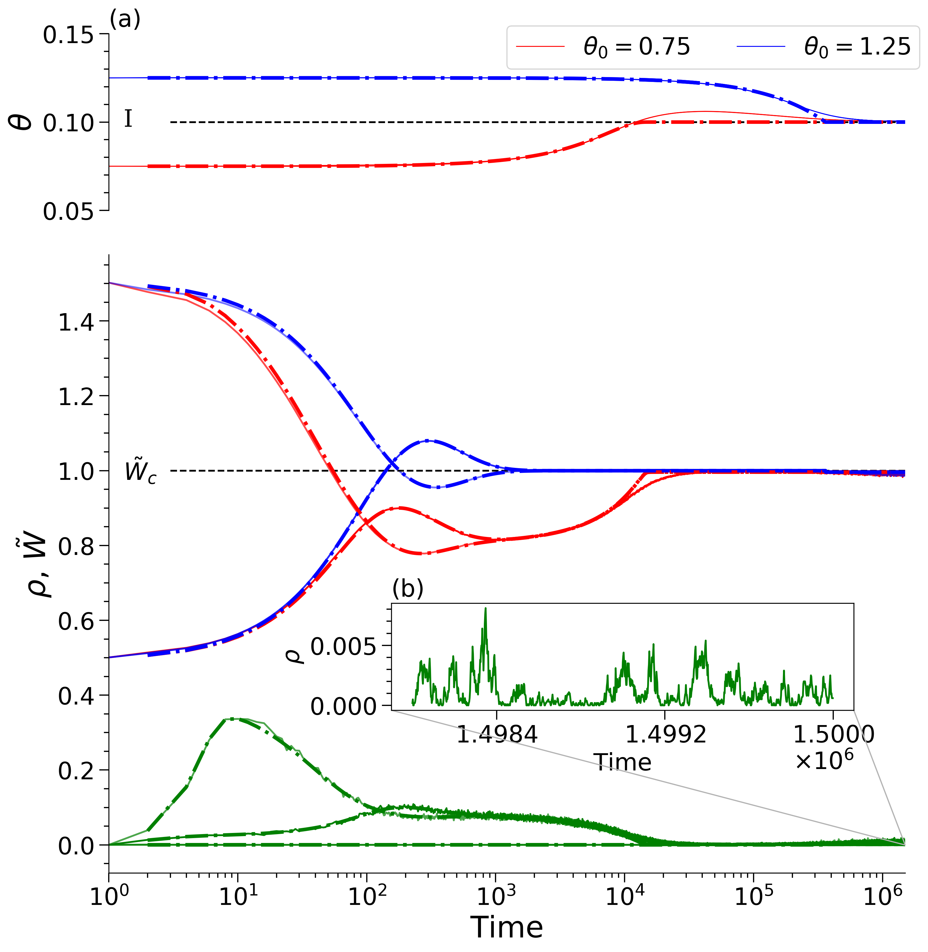
Figure 3: Self-organization of $\tilde{W}(t)$ and $\theta(t)$ from different initial conditions (blue and red). The target values are $\theta_{c}=I=0.1$ (or $h=I-\theta=0)$ and $\tilde{W}_{c}=1$. (a) Time series for $\theta(t)$ (top), $\tilde{W}(t)$ (middle) and $\rho(t)$ (green, bottom). Mean-field (dot-dash lines) and random network ($K=32$, solid lines) simulations with $N=10,000$ neurons. (b) Avalanche behavior for stationary $\rho(t)$. Parameters: $\tau_{W}=300$,$\tau_{\Gamma}=100$, $U_{W}=0.01$, $U_{\Gamma}=0.01$,$B=1$, $A=1$, $a=5000$ and $b=0.05$.

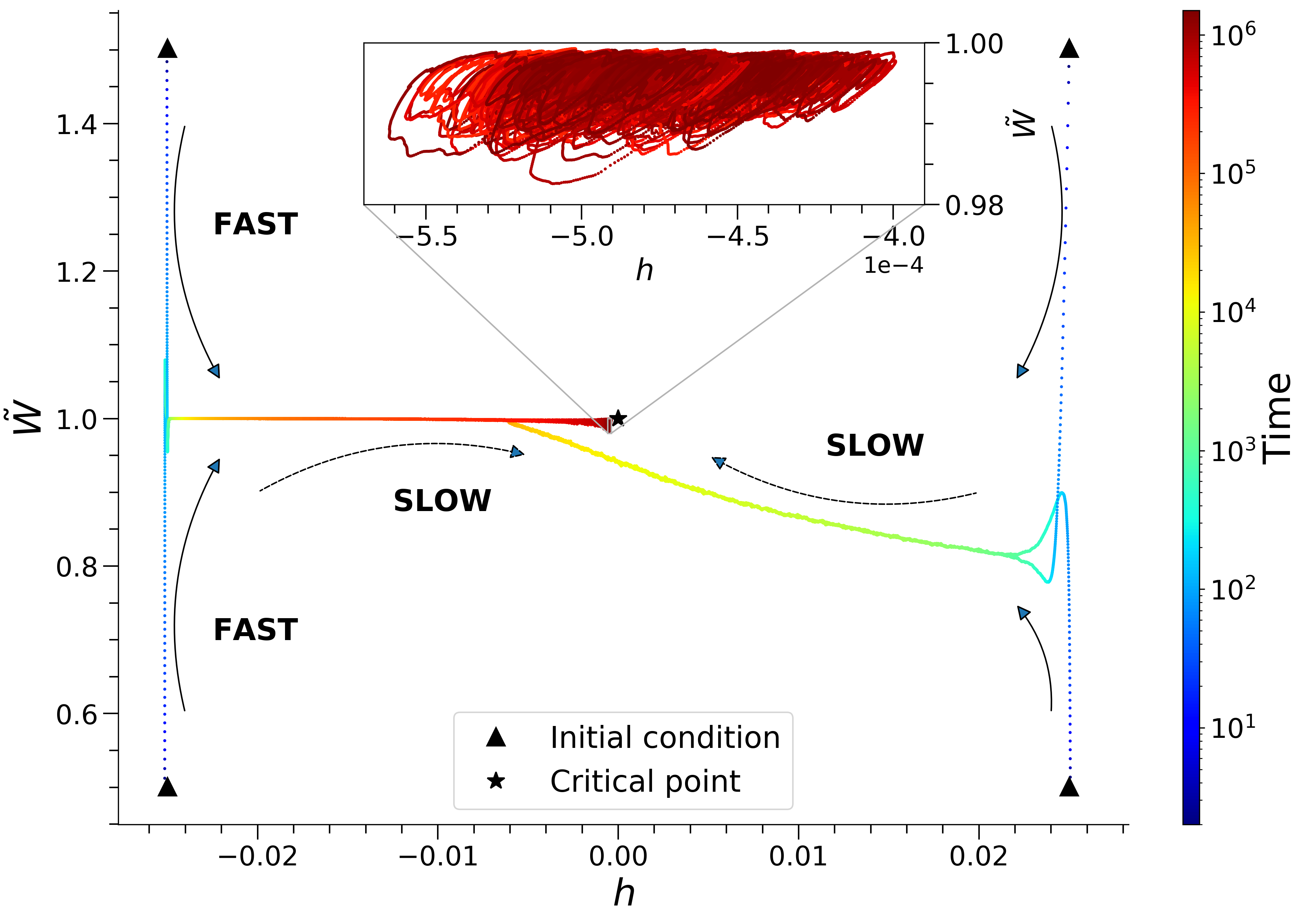
Figure 4: State space. Self-organization in the $\tilde{W}\times h$ plane for four different initial conditions (black triangles), input $I=0.1$, in a random network with $K=32$ and $N=10,000$ neurons. The temporal evolution of the system is indicated by the arrows and the color code (bluish hues correspond to the vicinity of initial conditions, while reddish to the steady state). Parameters: $\tau_{W}=300$, $\tau_{\Gamma}=100$, $U_{W}=0.01$, $U_{\Gamma}=0.01$, $a=5000$ and $b=0.05$.

We measured the size and duration of $10^{6}$ avalanche events after disregarding the transient activity. Avalanches are defined here as all activity between two consecutive visits to the absorbing state of the underlying static system ($\rho=0$) [35, 37]. In other words, we sum all spikes $N\rho(t)$ from all the time steps between two subsequent instants in which $\rho(t)$ is zero (i.e., all the activity in each peak between zeros of $\rho(t)$ in figure 3b). This method does not require thresholding the activity, as it makes use of the actual silent state of the network, thereby avoiding known biases in the estimation of avalanche exponents [38, 39, 40].

Near the critical point, we expect the avalanche sizes $s$ and duration $d$ to be distributed according to $F(s)=P(S>s)\sim s^{1-\tau}$ and $F(d)=P(D>d)\sim d^{1-\tau_{d}}$ respectively, with exponents $\tau=3/2$ and $\tau_{d}=2$ (exponents for a mean-field DP-like branching process [31, 34]). The $F(x)$ functions are the complementary cumulative distributions, which are defined as the integral of the distribution $P(X)$ over $X>x$. These distributions are a convenient choice since they are continuous functions that can be directly calculated from the data and do not rely on binning [41].

Having the correct exponents in the avalanche distributions is not a sufficient condition for identifying criticality [38, 42]. Therefore, we investigated the scaling law between mean avalanche size and duration $\left\langle s\right\rangle(d)$ leading to the scaling relation $m_{\text{theory}}=(\tau_{d}-1)/(\tau-1)$. At the underlying critical point (towards which the system is evolving), we have $m_{\text{theory}}=2$. In order to compare simulation results to the theory, we define the distance to criticality coefficient $dcc$ by: $dcc\equiv|m_{\text{theory}}-m_{\text{fitted}}|$, where the $m_{\text{fitted}}$ is given by directly fitting the data of $\left\langle s\right\rangle$ versus $d$. To compute the $dcc$, we take the mean value of $m_{\text{fitted}}$ adjusted to the simulation results with different $N$ for three values of $a$ and $b$.

The distributions of avalanche sizes and durations for the homeostatic system are presented in figure 5. In figure 6, we show how the finite-size scaling improves with increasing time scale separation $a$. Both the collapse of the curves is enhanced and the characteristic bump decreases as $a$ grows. Moreover, figure 7 shows that the exponent’s relation also tends to agree with the theory for increasing separation of time scales $a\to\infty$, resulting in a small distance to criticality ($dcc<0.01$) for $a=10^{6}$. These results show that the homeostatic mechanism proposed here is fully capable of approaching the underlying critical point ($\tau=3/2$, $\tau_{d}=2$ and $m=2$). This is different from other dynamics from the literature, since previous studies either lead to unclear avalanche distributions, or fail to reproduce the average size and duration scaling law.

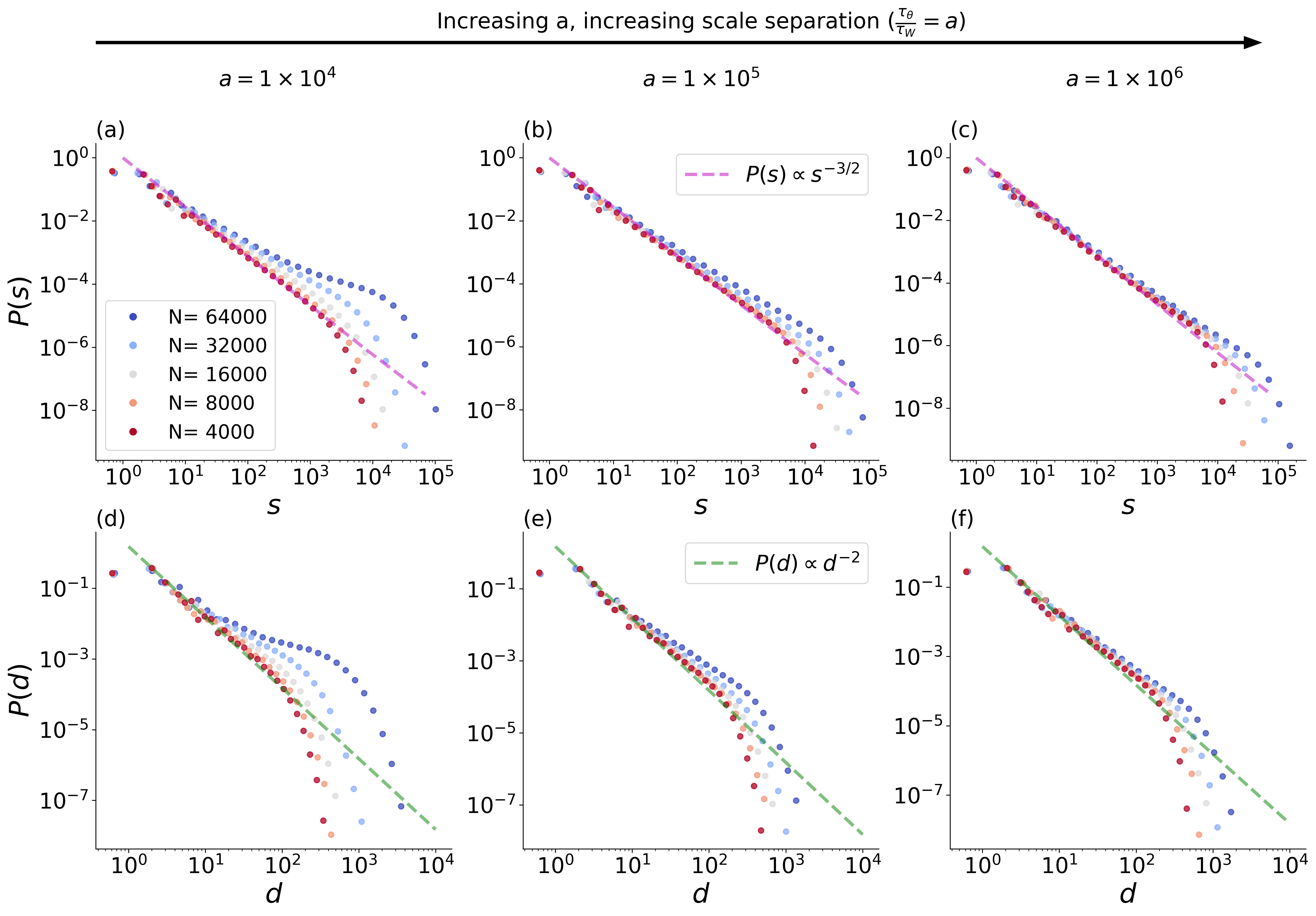
Figure 5: Power laws in avalanche sizes and duration distributions for increasing values of $a$ and network size $N$. The first and second rows show the distributions of sizes and duration, respectively. The agreement with the expected power laws (dashed lines) increases with $a$. Results obtained for a quenched simulation of a directed random network with $K=32$. Parameters: (a,d) $a=10^{4}$ and $b=8\times 10^{-2}$, (b,e) $a=10^{5}$ and $b=10^{-2}$ and (c,f) $a=10^{6}$ and $b=10^{-3}$.

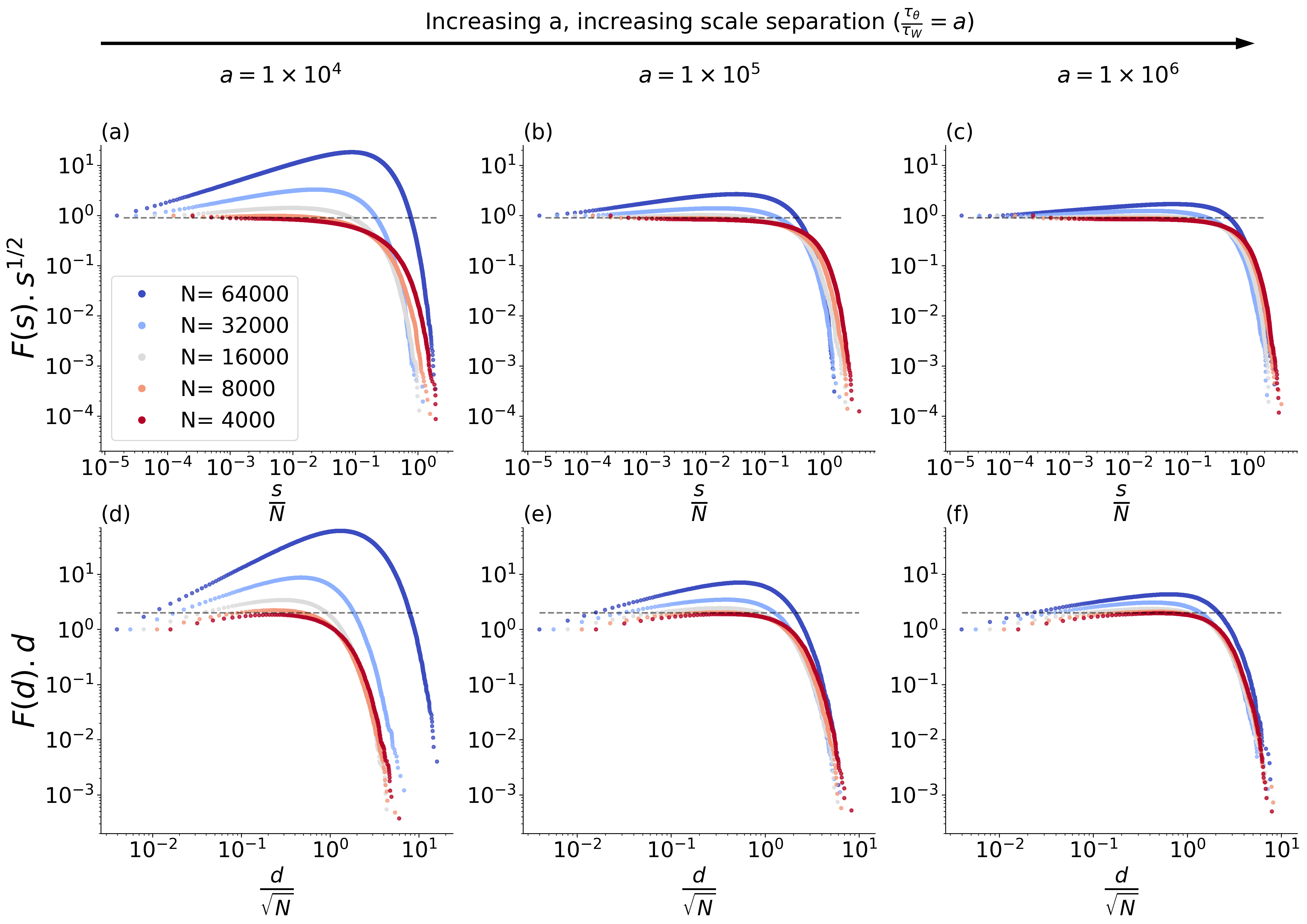
Figure 6: Finite-size scaling collapse of avalanche size and duration complementary cumulative distributions for increasing values of $a$ and network size $N$. The first row shows the collapse of the complementary cumulative distribution $F(s)$, and second row for duration, $F(d)$. The collapse improves with increasing $a$. Results obtained for a quenched simulation of a directed random network with $K=32$. Parameters: (a,d) $a=10^{4}$ and $b=8\times 10^{-2}$, (b,e) $a=10^{5}$ and $b=10^{-2}$ and (c,f) $a=10^{6}$ and $b=10^{-3}$.

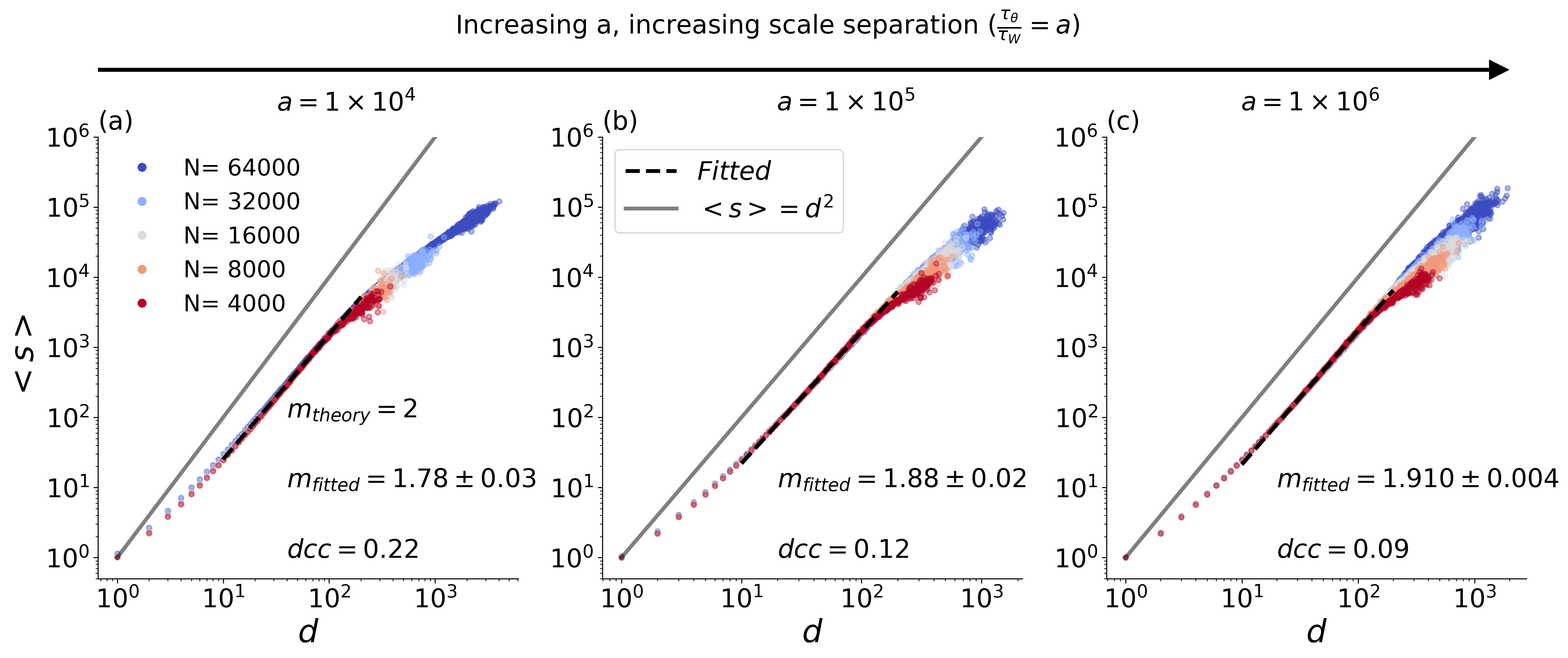
Figure 7: Average avalanche size vs. duration for increasing values of time scale separation $a$ and network size $N$. Directed random network with $K=32$. Average initial conditions: $\theta(0)=0.09$, $\Gamma(0)=0.75$ with $W(0)=1$, input $I=0.1$. (a) Parameters $a=10^{4}$ and $b=8\times 10^{-2}$; (b) $a=10^{5}$ and $b=10^{-2}$ and (c) $a=10^{6}$ and $b=10^{-3}$. Fitted exponent relation ($m_{\text{fitted}}$) and distance to criticality coefficient ($dcc=|m_{\text{theory}}-m_{\text{fitted}}|$) also shown.

The collapse of the avalanche size distribution can be calculated by, first, rescaling the variable through $u=s/s_{c}$, where $s_{c}=q_{1}N^{D}$ is the cutoff size of avalanches and $D$ is the size dimensionality (not to be confused with avalanche duration). Then, we define the scaling function $\mathcal{G}(u)=q_{2}s^{\tau}P(u)$. If the system is critical, this function will collapse the data from the simulations of different system sizes by plotting $\mathcal{G}(u)$ vs. $u$. The same can be achieved for the duration $d$, and for the cumulative distributions as well. The quantities $q_{1}$ and $q_{2}$ are called the metric coefficients; $q_{1}$ is obtained by collapsing the tail of the distributions on top of one another, and $q_{2}$ is obtained by fitting of a given distribution to the simulation data. These are not universal quantities, changing from one distribution to another [34]. For the avalanche exponents (and hence, criticality) to be well-defined, these coefficients must not depend on the system size $N$ [34]. In the data shown in figure 6, the failure of the collapse for small $a$ indicates that the metric coefficients depend on $N$. However, this happens in a non-trivial way, since the collapse enhances for increasing $a$. This tells us that the dependence on $N$ also becomes negligible in the growing $a$ limit, as the system gets closer and closer to the critical point. This is analytically supported by the form of the fixed points in equations (15)–(18); numerically by the $h$ amplitude in figure 2, as well as by the $dcc$ in figure 7.

The dependence of the metric coefficients on $N$ for small $a$ is expected due to the quasi-critical nature of our homeostatic system. We can explain it by the superposition of avalanches as follows. First, notice that the probability of uncorrelated spikes increases with $N$ since every neuron is an independent stochastic unit. These random spikes are spontaneously generated by the network due to a finite external field $h$, and they act as seeds to the avalanches. Therefore, the separation between events decreases with growing $N$ and, hence, avalanche superposition increases (see the Supplementary Information for more details). As our activity measure $\rho(t)$ cannot distinguish avalanches emerging from different seeds, this leads to an increased number of larger avalanches for larger $N$ (for more details, see the Supplementary Material). This effect vanishes for increasing $a$ because such regime promotes the separation of the internal time scales of the system. This in turn generates a decreasing effective external field $h\to 0$, ceasing simultaneous seeding of avalanches.

IV Discussion

We have presented a neuronal network model that self-organizes toward quasi-criticality, even in the presence of non-zero inputs $I_{i}$. This is an important result, given that cortical neurons, for example, are constantly bombarded by input from various areas. The homeostatic thresholds $\theta_{i}$ – which can also be interpreted as adaptation currents [43] – lead to $|h|<10^{-4}$, an (almost exact) adaptation to the inputs. That is, instead of imposing $h=0$ as is usually done in standard SOC models [4], here we construct homeostatic mechanisms such that the effective fields $h_{i}(t)=I_{i}-\theta_{i}(t)$ tend towards zero. This is no mere detail, but a crucial ingredient for a truly self-organized critical model [4].

The $\tilde{W}^{*}$ component of the fixed point is always subcritical, but tends to the critical value when $ab\to\infty$. From a biological perspective, staying in the vicinity of a subcritical state might be advantageous to decrease the risk of spontaneous runaway activity [44]. Such activity could be linked to dysfunctional regimes like epilepsy. Also, from the perspective of information processing and task performance, it was recently shown that while criticality might be beneficial for complex computational tasks, it can be detrimental to the performance in simpler ones [45]. This suggests that the subcriticality expressed by our model, with just a few excursions to a critical state for some particular tasks, might be the best regime for the network.

The form of the adaptation currents adopted for thresholds $\theta_{i}$ is known to generate negative correlations between consecutive interspike intervals [46]. This means that long silent intervals will be followed by shorter ones, on average. In addition, experimental results suggest that large avalanche-like events are followed, on average, by small events in the resting state of the brain [47]. Thus, the adaptation to the external field displayed by our model could be the mechanism responsible for the generation of the separation between time scales. This separation has to be imposed in all classic SOC models, but emerges naturally in our model for large $a$.

After the self-organization process, the system hovers around a stable (quasi-critical) fixed point with small amplitude orbits, minimizing the large stochastic oscillations observed in previous models [16, 18, 20]. In particular, the system gets closer to criticality as the timescale ratio $a=\tau_{\theta}/\tau_{W}=\tau_{\theta}/\tau_{\Gamma}$ increases. This effect is related to the decrease of the effective external field $h$. In turn, this vanishing $h$ is what restores the true scaling and power laws in the avalanche distributions as the separation of time scale grows. This is because both $a\to\infty$ and $h\to 0$ are required to suppress the superposition of avalanches.

Self-organization mechanisms that tune neuronal networks to various states based on the homeostatic interplay of external input and intrinsic activity have already been explored in the literature [48]. However, scale-free avalanches with mean-field DP-like exponents that satisfy the scaling relation had been only observed in the limit of vanishing external drive [24]. In our model, both the exponents and the scaling arise naturally from the adaptation mechanism.

Regarding the unavoidable fine-tuning $A\approx 1$ imposed in our study, we need to remember Hernandez-Urbina and Herrmann [49, 22]: fine-tuning a hyperparameter in local homeostatic mechanisms is very different from globally fine-tuning the parameters $\{W_{ij},h_{i}\}$ in the original static model. In any case, a challenge to the community persists: is it possible to obtain $A\approx 1$ without any form of fine-tuning? We conjecture that this is impossible: the need for $h^{*}\approx 0$ will impose strict conditions similar to $A\approx 1$ to any other homeostatic model [21].

Generalizing our results, it is plausible that any system under the influence of external fields (say, a magnetic field $H$ in spin systems) – as in earthquakes, forest fires, voting or epidemic models based on spins, cellular automata or even continuous time integrate-and-fire dynamics – can achieve a near-critical regime through the inclusion of adaptive local fields (as our $\theta_{i}(t)$) whose timescale should be much slower than that of the rest of the system.

Nonetheless, it is not clear how time-varying inputs $I_{i}(t)$ would affect the behavior of our system. We conjecture that the thresholds $\theta_{i}(t)$ would produce a phenomenon akin to sensory adaptation [50, 51]. If so, for short time scales, our homeostatic networks would respond to the derivatives of the external signal, as opposed to signal intensity. This could lead to yet unknown computational properties. For example, the results on the optimization of the dynamic range in critical networks [52] could be challenged, or, at least, would need to be reconsidered in the context of sensory systems with adaptation. This important issue will be studied in a future extended paper.

V Acknowledgments

G.M. would like to thank CAPES for financial support. M.G.-S. thanks the financial support of NSERC grant BCPIR/493076-2017 from A. Longtin and L. Maler. O.K. acknowledges CNAIPS-USP and CNPq, Conselho Nacional de Desenvolvimento Científico e Tecnológico support. This work was produced as part of the activity of FAPESP Research, Innovation and Dissemination Center for Neuromathematics (grant #2013/07699-0 S. Paulo Research Foundation).

References

- [1] Per Bak, Chao Tang, and Kurt Wiesenfeld. Self-organized criticality: An explanation of the 1/f noise. Phys. Rev. Lett., 59(4):381, 1987.
- [2] Henrik Jeldtoft Jensen. Self-organized criticality: Emergent Complex Behavior in Physical and Biological Systems. Cambridge Univ. Press, Cambridge, UK, 1998.
- [3] Ronald Dickman, Alessandro Vespignani, and Stefano Zapperi. Self-organized criticality as an absorbing-state phase transition. Phys. Rev. E, 57(5):5095, 1998.
- [4] Ronald Dickman, Miguel A Muñoz, Alessandro Vespignani, and Stefano Zapperi. Paths to self-organized criticality. Braz. J. Phys., 30(1):27–41, 2000.
- [5] Juan A Bonachela and Miguel A Muñoz. Self-organization without conservation: true or just apparent scale-invariance? J. Stat. Mech., 2009(09):P09009, 2009.
- [6] Victor Buendia, Serena di Santo, Juan A. Bonachela, and Miguel A. Muñoz. Feedback mechanisms for self-organization to the edge of a phase transition. Frontiers in Physics, 8:333, 2020.
- [7] John M Beggs and Dietmar Plenz. Neuronal avalanches in neocortical circuits. J. Neurosci., 23(35):11167–11177, 2003.
- [8] John M Beggs. The criticality hypothesis: how local cortical networks might optimize information processing. Philos. Trans. R. Soc. A, 366(1864):329–343, 2008.
- [9] D R Chialvo. Emergent complex neural dynamics. Nature Phys., 6(10), 2010.
- [10] M A Muñoz. Colloquium: Criticality and dynamical scaling in living systems. Rev. Mod. Phys., 90(3), 2018.
- [11] Tawan T. A. Carvalho, Antonio J. Fontenele, Mauricio Girardi-Schappo, Thaís Feliciano, Leandro A. A. Aguiar, Thais P. L. Silva, Nivaldo A. P. de Vasconcelos, Pedro V. Carelli, and Mauro Copelli. Subsampled directed-percolation models explain scaling relations experimentally observed in the brain. Frontiers in Neural Circuits, 14:83, 2021.
- [12] Anna Levina, J Michael Herrmann, and Theo Geisel. Dynamical synapses causing self-organized criticality in neural networks. Nature Phys., 3(12):857–860, 2007.
- [13] Juan A Bonachela, Sebastiano de Franciscis, Joaquín J Torres, and Miguel A Muñoz. Self-organization without conservation: are neuronal avalanches generically critical? J. Stat. Mech., 2010(02):P02015, 2010.
- [14] Roxana Zeraati, Viola Priesemann, and Anna Levina. Self-Organization Toward Criticality by Synaptic Plasticity. Frontiers in Physics, 9(April):1–17, 2021.
- [15] L Brochini, A A Costa, M Abadi, A C Roque, J Stolfi, and O Kinouchi. Phase transitions and self-organized criticality in networks of stochastic spiking neurons. Sci. Rep., 6, 2016.
- [16] A A Costa, L Brochini, and O Kinouchi. Self-organized supercriticality and oscillations in networks of stochastic spiking neurons. Entropy, 19(8):399, 2017.
- [17] João G F Campos, Ariadne A Costa, M Copelli, and O Kinouchi. Correlations induced by depressing synapses in critically self-organized networks with quenched dynamics. Phys. Rev. E, 95:042303, 2017.
- [18] Osame Kinouchi, Ludmila Brochini, Ariadne A Costa, Campos. João G F, and Mauro Copelli. Stochastic oscillations and dragon king avalanches in self-organized quasi-critical systems. Sci. Rep., 9:3874, 2019.
- [19] Bruno Del Papa, Viola Priesemann, and Jochen Triesch. Criticality meets learning: Criticality signatures in a self-organizing recurrent neural network. PLoS One, 12:e0178683, 2017.
- [20] M Girardi-Schappo, Brochini L, A A Costa, T T A Carvalho, and O Kinouchi. Synaptic balance due to homeostatically self-organized quasi-critical dynamics. Phys. Rev. Research, 2:012042, 2020.
- [21] M. Girardi-Schappo, E. F. Galera, T. T. A. Carvalho, L. Brochini, N. L. Kamiji, A. C. Roque, and O. Kinouchi. A unified theory of E/I synaptic balance, quasicritical neuronal avalanches and asynchronous irregular spiking. J Phys Complex, page in press, 2021.
- [22] Osame Kinouchi, Renata Pazinni, and Mauro Copelli. Mechanisms of self-organized quasicriticality in neuronal networks models. Front. Phys., 8, 2020.
- [23] Rashid V. Williams-García, Mark Moore, John M. Beggs, and Gerardo Ortiz. Quasicritical brain dynamics on a nonequilibrium Widom line. Physical Review E - Statistical, Nonlinear, and Soft Matter Physics, 90(6):1–8, 2014.
- [24] Antonio de Candia, Alessandro Sarracino, Ilenia Apicella, and Lucilla de Arcangelis. Critical behaviour of the stochastic Wilson-Cowan model. PLOS Computational Biology, 17(8):e1008884, aug 2021.
- [25] W Gerstner and J L van Hemmen. Associative memory in a network of ‘spiking’ neurons. Netw. Comput. Neural Syst., 3(2), 1992.
- [26] A Galves and E Löcherbach. Infinite systems of interacting chains with memory of variable length — a stochastic model for biological neural nets. J. Stat. Phys., 151(5), 2013.
- [27] Daniel B Larremore, Woodrow L Shew, Edward Ott, Francesco Sorrentino, and Juan G Restrepo. Inhibition causes ceaseless dynamics in networks of excitable nodes. Phys. Rev. Lett., 112(13):138103, 2014.
- [28] Johannes Zierenberg, Jens Wilting, Viola Priesemann, and Anna Levina. Tailored ensembles of neural networks optimize sensitivity to stimulus statistics. Phys. Rev. Research, 2(1):013115, 2020.
- [29] Mauricio Girardi-Schappo and M. H. R. Tragtenberg. Comment on “Convergence towards asymptotic state in 1-D mappings: A scaling investigation”. Phys. Lett. A, 383(36):126031, 2019.
- [30] John M Beggs and Dietmar Plenz. Neuronal avalanches are diverse and precise activity patterns that are stable for many hours in cortical slice cultures. J. Neurosci., 24(22):5216–5229, 2004.
- [31] Malte Henkel, Haye Hinrichsen, and Sven Lübeck. Non-Equilibrium Phase Transitions. Volume I: Absorbing Phase Transitions. Theoretical and Mathematical Physics. Springer Netherlands, Dordrecht, 2008.
- [32] N Spruston, Y Schiller, G Stuart, and B Sakmann. Activity-dependent action potential invasion and calcium influx into hippocampal CA1 dendrites. Science, 268(5208):297–300, apr 1995.
- [33] Leonardo L Gollo, Osame Kinouchi, and Mauro Copelli. Active dendrites enhance neuronal dynamic range. PLos Comput. Biol., 5(6):e1000402, 2009.
- [34] Gunnar Pruessner. Self-Organised Criticality, volume 54. Cambridge University Press, Cambridge, jun 2012.
- [35] Miguel A. Muñoz, Ronald Dickman, Alessandro Vespignani, and Stefano Zapperi. Avalanche and spreading exponents in systems with absorbing states. Phys. Rev. E, 59(5):6175, 1999.
- [36] Anh-Tuan Trinh, Mauricio Girardi-Schappo, Jean-Claude Béïque, André Longtin, and Leonard Maler. Dentate gyrus mossy cells exhibit adaptive spike threshold dynamics. In preparation, 2022.
- [37] Mauricio Girardi-Schappo and Marcelo H. R. Tragtenberg. Measuring neuronal avalanches in disordered systems with absorbing states. Phys. Rev. E, 97:042415, 2018.
- [38] Jonathan Touboul and Alain Destexhe. Power-law statistics and universal scaling in the absence of criticality. Physical Review E, 95:012413, 2017.
- [39] Serena di Santo, Pablo Villegas, Raffaella Burioni, and Miguel A Muñoz. Landau–Ginzburg theory of cortex dynamics: Scale-free avalanches emerge at the edge of synchronization. Proc. Natl. Acad. Sci. USA, 115(7):E1356–E1365, 2018.
- [40] Pablo Villegas, Serena Di Santo, Raffaella Burioni, and Miguel A. Muñoz. Time-series thresholding and the definition of avalanche size. Physical Review E, 100(1):1–6, 2019.
- [41] Mauricio Girardi-Schappo, Osame Kinouchi, and Marcelo H R Tragtenberg. Critical avalanches and subsampling in map-based neural networks coupled with noisy synapses. Phys. Rev. E, 88(2):024701, 2013.
- [42] Mauricio Girardi-Schappo. Brain criticality beyond avalanches: open problems and how to approach them. J Phys Complex, 2:031003, 2021.
- [43] Jan Benda, Leonard Maler, and André Longtin. Linear versus nonlinear signal transmission in neuron models with adaptation currents or dynamic thresholds. Journal of Neurophysiology, 104(5):2806–2820, 2010.
- [44] V Priesemann. Self-organization to sub-criticality. BMC Neuroscience, 16(S1):O19, dec 2015.
- [45] Benjamin Cramer, David Stöckel, Markus Kreft, Michael Wibral, Johannes Schemmel, Karlheinz Meier, and Viola Priesemann. Control of criticality and computation in spiking neuromorphic networks with plasticity. Nature Communications, 11(1):2853, dec 2020.
- [46] William H. Nesse, Leonard Maler, and André Longtin. Enhanced Signal Detection by Adaptive Decorrelation of Interspike Intervals. Neural Computation, 33:341–375, 2021.
- [47] F. Lombardi, D.R. Chialvo, H.J. Herrmann, and L. de Arcangelis. Strobing brain thunders: Functional correlation of extreme activity events. Chaos Solitons Fractals, 55:102–108, 2013.
- [48] Johannes Zierenberg, Jens Wilting, and Viola Priesemann. Homeostatic Plasticity and External Input Shape Neural Network Dynamics. Physical Review X, 8(3):31018, 2018.
- [49] Victor Hernandez-Urbina and J. Michael Herrmann. Self-organized Criticality via Retro-Synaptic Signals. Frontiers in Physics, 4, jan 2017.
- [50] Thomas Petermann, Tara C. Thiagarajan, Mikhail A. Lebedev, Miguel A. L. Nicolelis, Dante R. Chialvo, and Dietmar Plenz. Spontaneous cortical activity in awake monkeys composed of neuronal avalanches. Proceedings of the National Academy of Sciences, 106(37):15921–15926, sep 2009.
- [51] Gerald Hahn, Thomas Petermann, Martha N. Havenith, Shan Yu, Wolf Singer, Dietmar Plenz, and Danko Nikolić. Neuronal Avalanches in Spontaneous Activity In Vivo. Journal of Neurophysiology, 104(6):3312–3322, dec 2010.
- [52] Osame Kinouchi and Mauro Copelli. Optimal dynamical range of excitable networks at criticality. Nature Phys., 2(5):348–351, 2006.