Decentralized Stability Conditions for DC Microgrids: Beyond Passivity Approaches

Abstract

We consider the problem of ensuring stability in a DC microgrid by means of decentralized conditions. Such conditions are derived which are formulated as input-output properties of locally defined subsystems. These follow from various decompositions of the microgrid and corresponding properties of the resulting representations. It is shown that these stability conditions can be combined together by means of appropriate homotopy arguments, thus reducing the conservatism relative to more conventional decentralized approaches that often rely on a passivation of the bus dynamics. Examples are presented to demonstrate the efficiency and the applicability of the results derived.

I Introduction

The increasing integration of renewable energy in recent years has strengthened the interest in microgrids. Compared to AC microgrids, DC microgrids have been recognized as a natural and simple solution to integrate renewable energy, see [1]. For instance, DC microgrids allow connecting DC components directly for a simple integration of renewable generation and storage units. Moreover, in addition to being compatible with modern consumer loads, DC microgrids allow to reduce unnecessary power conversion losses. Thus, DC microgrids have become an attractive option not only for providing support to remote communities, but in many other applications such as mobile grids on ships, aircrafts, and trains [2].

A DC microgrid is a power network that consists of small subsystems (generation units, storage units, flexible loads, etc.) interconnected via power lines. A key requirement in a DC microgrid is to ensure stability of the network when decentralized feedback control mechanisms are used for voltage/current regulation [3].

Two main features can lead to network instability: interaction between converters and load type, see [3, 4].

In particular, each DC-DC converter is typically designed to guarantee good stability margins and achieve certain performance levels when operating in a stand-alone condition. However, when interconnecting the different DC-DC converters in the network, their interaction can affect the overall performance and even lead to instability.

Furthermore, some DC loads have a destabilizing effect. For instance, in contrast to constant impedance loads and constant current loads, which normally do not induce stability degradation, constant power loads can lead to network instability due to their negative impedance characteristics.

I-A Literature review

Various decentralized (linear and nonlinear) control strategies have been proposed in the literature to ensure proper functioning of DC microgrids: droop control schemes [5, 6], line-independent approaches [7], cooperative schemes [8] , passivity-based [9, 10], Lyapunov-based [11], backstepping [12], and sliding-mode control schemes [13].

However, the aforementioned controllers do not handle situations where constant power loads are present and some of them do not incorporate the power line dynamics and consider them purely resistive.

To address the voltage destabilizing effect of constant power loads, various controllers have been proposed in the literature to handle general nonlinear ZIP loads, i.e. parallel combination of constant impedance, current, and power load respectively (denoted as Z, I, P respectively).

In [14], the authors propose a consensus algorithm guaranteeing power consensus in a network with ZIP loads. In [15], the authors propose a nonlinear passivity based voltage controller with some robustness with respect to constant ZIP loads. In [16], the authors propose a linear state feedback voltage controller to passivate the generation units and the ZIP loads connected to it.

Existing results that incorporate dynamic line models rely primarily on a passivation of the bus dynamics so as to achieve stability in general network topologies. The latter implies that there are restrictions on the amount of constant power loads that can be incorporated, as these have a non-passive behaviour. Furthermore, many classical converter control architectures, such as ones based on double-loop implementations that provide also current control capabilities, are often hard to passivate in practical designs. Therefore the development of methodologies that can reduce the conservatism in the stability conditions imposed, while at the same having stability guarantees in general network topologies is an important problem of practical relevance.

I-B Main contributions

The objective of this paper is to derive decentralized conditions through which stability of the DC microgrid can be established, i.e. conditions on locally defined subsystems. The microgrid representation plays a central role in this context as the notion of a subsystem is not unique. In particular, any derived stability conditions are inevitably going to be only sufficient when these are decentralized. Therefore, different representations of what constitutes a subsystem within the network can lead to stability results with varying conservatism.

A main idea of our analysis is to consider different decentralized input-output conditions based on various decompositions of a DC network and then combine them together by means of appropriate homotopy arguments. This allows to exploit on the one hand the natural passivity properties of the lines in frequency ranges where the coupling between the buses is high, and also exploit other input-output conditions in frequency ranges where there are significant deviations from passivity by additionally taking into account the strength of the coupling between buses.

A key contribution of the proposed approach is that it allows to reduce the conservatism in the design relative to more conventional methodologies, such as ones that rely on a passivation of bus dynamics. In particular, it enables larger amounts of constant power loads to be incorporated while guaranteeing stability of the network, and also allows to establish stability for wider classes of practically relevant control architectures.

It should also be noted that the input-output approach adopted allows to consider broad classes of microgrid models involving higher order converter models and line dynamics. Related practical examples will also be discussed within the paper to demonstrate the significance of the results presented.

I-C Paper outline

The paper is structured as follows. Section II presents some graph theory elements, the DC microgrid model and the problem setting. Section III presents the main results of the paper while Section IV presents numerical examples. Conclusions are drawn in Section V.

I-D Symbols and notations

The sets of real and complex numbers are denoted by $\mathbf{R}$ and $\mathbf{C}$ respectively. The extended real line $\left[-\infty,+\infty\right]$ is denoted $\overline{\mathbf{R}}$ and $\overline{\mathbf{R}}_{+}$ is the set of real positive numbers including 0 and $+\infty$. The imaginary axis is denoted by $\mathbf{j}\overline{\mathbf{R}}$ where $\mathbf{j}=\sqrt{-1}$. The right half-plane including the imaginary axis is denoted by ${\mathbf{C}}_{+}$ and its closure is denoted by $\overline{\mathbf{C}}_{+}$. The space $\mathscr{L}_{2}^{n}[0,\infty)$ is the set of signals $f:[0,\infty)\rightarrow\mathbf{R}^{n}$ that have finite energy $\int_{0}^{\infty}\|f(t)\|^{2}\text{d}t$, and $\mathscr{H}^{n}_{2}$ is the set of functions that are Laplace transforms of signals in $\mathscr{L}_{2}^{n}[0,\infty)$. The set $\mathbb{RH}_{\infty}^{p\times q}$ is the set of ${p\times q}$ real rational transfer functions without poles in $\overline{\mathbf{C}}_{+}$. For a matrix $F\in\mathbf{C}^{n\times n}$ its transpose and conjugate transpose are denoted by $F^{\top}$ and $F^{*}$ respectively. For a matrix $F\in\mathbf{C}^{m\times n}$, $\|F\|_{\infty}$, $\rho(F)$ denote its induced $\infty$-norm and its spectral radius respectively. The identity matrix is denoted by $I$.The Kronecker product of two matrices $F_{i}$ and $F_{j}$ is denoted by $F_{i}\otimes F_{j}$. The direct sum of matrices $F_{i}$ with $i=1,\cdots,n$ is denoted by $\oplus_{i=1}^{n}F_{i}$. Finally, in order to ease the notation, for matrices $X,\Pi_{11},\Pi_{12},\Pi_{22}$ with compatible dimensions and $\epsilon\geq 0$, we use $X\in\mbox{$\bf{QC}$}\left(\Pi,\epsilon\right)$, with $\Pi=\begin{pmatrix}\Pi_{11}&\Pi_{12}\\ \Pi_{12}^{*}&\Pi_{22}\end{pmatrix}$, to denote

$$\begin{pmatrix}X\\ I\end{pmatrix}^{*}\leavevmode\nobreak\ \leavevmode\nobreak\ \Pi\leavevmode\nobreak\ \leavevmode\nobreak\ \begin{pmatrix}X\\ I\end{pmatrix}\geq\epsilon X^{*}X$$ (1)

and $X\in\mbox{$\overline{\bf{QC}}$}\left(\Pi,\bar{\epsilon}\right)$ to denote

$$\begin{pmatrix}I\\ -X\end{pmatrix}^{*}\leavevmode\nobreak\ \leavevmode\nobreak\ \Pi\leavevmode\nobreak\ \leavevmode\nobreak\ \begin{pmatrix}I\\ -X\end{pmatrix}\leq-\bar{\epsilon}I.$$

II Network models and problem setting

II-A Algebraic graph theory and microgrid signals

The DC microgrid is a power system that comprises of $n_{b}$ buses and $n_{\ell}$ power lines. We assume that each bus includes a DC-DC converter with its controller, and a load connected to it. Note that even if loads are located elsewhere, they can be mapped to a point of common coupling (PCC) using Kron reduction, see [17]. Fig. 1 is a representative diagram of a microgrid with six buses and six lines while Fig. 2 gives a schematic of the electrical connection of the $j^{th}$ bus.

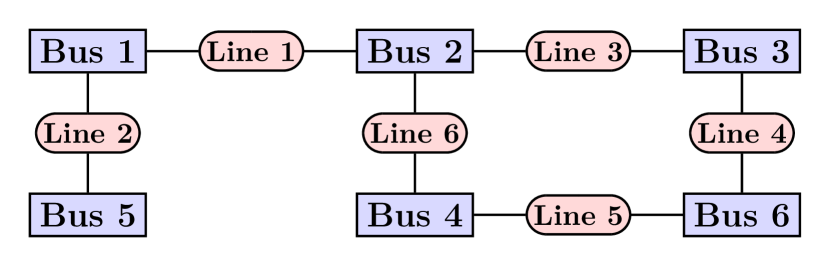
Figure 1: A representative diagram of a six bus microgrid.

Figure 2: Diagram representing the $j^{th}$ bus (DC-DC converter with its controller, and a load) connected to the $k^{th}$ line.

We represent this microgrid as a connected graph $(\mathcal{N},\mathcal{E})$ where $\mathcal{N}=\left\{1,2,\cdots,n_{b}\right\}$ is the set of nodes (buses) and $\mathcal{E}=\left\{1,\cdots,n_{\ell}\right\}\subseteq\mathcal{N}\times\mathcal{N}$ is the set of edges (lines). A direction is assigned to each edge which can be arbitrarily chosen. The corresponding $n_{b}\times n_{\ell}$ incidence matrix is denoted by $\mathcal{A}$ and it is given by

$$\mathcal{A}_{jk}=\left\{\begin{matrix}&+1&\text{if edge $k$ leaves bus $j$,}\\ &-1&\text{if edge $k$ enters bus $j$,}\\ &\leavevmode\nobreak\ \leavevmode\nobreak\ 0&\text{otherwise.\leavevmode\nobreak\ \leavevmode\nobreak\ \leavevmode\nobreak\ \leavevmode\nobreak\ \leavevmode\nobreak\ \leavevmode\nobreak\ \leavevmode\nobreak\ \leavevmode\nobreak\ \leavevmode\nobreak\ \leavevmode\nobreak\ \leavevmode\nobreak\ \leavevmode\nobreak\ \leavevmode\nobreak\ \leavevmode\nobreak\ }\\ \end{matrix}\right.$$

For each node $j\in\mathcal{N}$, the set $\mathcal{E}_{j}=\left\{k\in\mathcal{E}:\mathcal{A}_{jk}\neq 0\right\}$ is the set of edges connected to node $j$.

Given the aforementioned microgrid settings, we define the following signals.

• The input current at bus $j$ is denoted by $i_{B_{j}}(t)$ and the bus output voltage is denoted by $v_{B_{j}}(t)$.

• The current through line $k$ is denoted by $i_{L_{k}}(t)$ (this denotes the current with the same direction as that of the edge $k$).

• The vector of all bus voltages and the vector of all line currents are denoted by $v_{B}(t)=\left(v_{B_{j}}(t)\right)_{j\in\mathcal{N}}$ and $i_{L}(t)=\left(i_{L_{k}}(t)\right)_{k\in\mathcal{E}}$ respectively.

II-B Line dynamics

We consider power lines modeled as RL components. The lines of the DC microgrid connect the buses and allow power to be transferred from one bus to another and across the microgrid as a whole. The current flowing across a line is determined by the difference between the voltages at each bus to which the line is connected. By applying Kirchoff’s voltage law on the $k^{th}$ power line, with $k\in\mathcal{E}$, we obtain

$$\diff{i_{L_{k}}(t)}{t}=\dfrac{-r_{k}}{l_{k}}i_{L_{k}}(t)+\dfrac{1}{l_{k}}\delta V_{L_{k}}(t)$$ (2)

where $r_{k}>0$ and $l_{k}>0$ are the resistance and the inductance of $k^{th}$ line and $\delta V_{L_{k}}(t)$ is the voltage difference across line $L_{k}$.

It should be noted though that the stability results that will be presented also hold if the transfer function from $\delta V_{L_{k}}$ to $i_{L_{k}}$ is any strictly positive real function. This allows, for example, to consider also more advanced line models that include capacitances or distributed parameter models as in [18]. Extensions to cases where this transfer function is positive real rather than strictly positive real, will also be considered in Theorem 2.

II-C Bus dynamics

As already mentioned, each bus includes a DC-DC converter with its own controller, and a load connected to it. The voltage at each bus is controlled via the DC-DC converter using local information only (i.e. the states of the bus and the input current from the microgrid).

We consider a general bus model to account for a broad class of DC-DC converters, controllers and loads. DC-DC converters (buck, boost, buck-boost, SEPIC, etc.) are composed of three main stages: DC stage (battery stage), switching stage and DC output stage (output-voltage stage).

Average models, i.e. models described by continuous ODEs, are commonly used in the literature to describe the converter dynamics so as to carry out stability analysis and control design. These are justified under the following assumption.

Assumption 1.

The switching of the converter is performed at a frequency much higher than the timescale of its control policies.

Thereafter, average models will be used throughout the paper to model the converter dynamics.

The converter dynamics as well as the controller dynamics vary depending on the DC microgrid voltage level (low, medium and high), model complexity, control strategy, etc.. Therefore, the converter and the controller dynamics will be kept in a general representation for analysis and particular implementations will be discussed in the examples of Section IV. For the loads, we consider a general ZIP load model which includes constant impedance, constant current and constant power loads.

A general form of the $j^{th}$ bus dynamics can be described as single-input single-output dynamical system with $i_{B_{j}}(t)$ as input and $v_{B_{j}}(t)$ as output. These dynamics are represented as follows

$$\left\{\begin{matrix}&\diff{x_{B_{j}}(t)}{t}=f_{B_{j}}\big{(}x_{B_{j}}(t),i_{B_{j}}(t)\big{)}\\ &\leavevmode\nobreak\ \leavevmode\nobreak\ v_{B_{j}}(t)=g_{B_{j}}\big{(}x_{B_{j}}(t),i_{B_{j}}(t)\big{)}\end{matrix}\right.$$ (3)

where $x_{B_{j}}(t)\in\mathbf{R}^{{n_{x_{B_{j}}}}}$ is the state vector at each bus (includes converter, controller, and load states), $f_{B_{j}}$ and $g_{B_{j}}$ are functions of the form $f_{B_{j}}:\mathbf{R}^{{n_{x_{B_{j}}}}}\times\mathbf{R}\rightarrow\mathbf{R}^{{n_{x_{B_{j}}}}}$ and $g_{B_{j}}:\mathbf{R}^{{n_{x_{B_{j}}}}}\times\mathbf{R}\rightarrow\mathbf{R}$.

II-D Microgrid small-signal model

The bus model (3) is in general nonlinear due to the converter and load dynamics even when considering linear controllers; hence the microgrid model is also nonlinear. Equilibrium points can be found by setting the time derivatives in (2)-(3) to zero and then solving the resulting system of equations.

Finding equilibrium points in a power grid is the well-known power-flow problem, which has been studied in depth e.g. [19, 20]. Load / generation fluctuations result in deviations from a nominal operating point, however when these are small, which is usually the case under normal operating conditions, a small signal analysis can be used for stability analysis and control design.

Thereafter, a linearization is performed using an obtained equilibrium. For this purpose, we require the following assumption.

Assumption 2.

The system (2)-(3) admits an equilibrium. Moreover, the vector functions $f_{B_{j}}$ and the functions $g_{B_{j}}$ in (3) are Lipschitz around the considered equilibrium of (2)-(3).

Under Assumption 2, the system (2)-(3) can be linearized about the equilibrium being considered. In order to analyze this linearization, let $\overline{q}(t)=q(t)-q^{eq}$ denote the deviation of any quantity $q(t)$ from its equilibrium value $q^{eq}$. We denote the microgrid equilibrium by $q^{eq}$ given by

$$q^{eq}=\begin{pmatrix}\big{(}i_{L}^{eq}\big{)}^{\top},&\big{(}v_{B}^{eq}\big{)}^{\top},&\big{(}x_{B}^{eq}\big{)}^{\top}\end{pmatrix}^{\top}$$ (4)

with $x_{B}^{eq}=(x^{eq}_{B_{j}})_{j\in\mathcal{N}}$. Finally, we adopt an input-output representation of the small-signal model of microgrid (2)-(3), and we introduce the following two sets of transfer functions

• $L_{k}(s)$ is the transfer function of the line dynamics (2), from the input $\overline{\delta V_{L_{k}}}(t)$ to the output $\overline{i_{L_{k}}}(t)$;

• $B_{j}(s)$ is the transfer function of the linearized version of the bus dynamics (3) from the input $\overline{i_{B_{j}}}(t)$ to the output $\overline{v_{B_{j}}}(t)$.

Note that the different $L_{k}(s)$, obtained from (2), are in $\mathbb{RH}_{\infty}$ as $-r_{k}l_{k}^{-1}<0$. We will derive conditions on the frequency response of locally defined subsystems under which stability of the power system (2)-(3) about the equilibrium (4) is guaranteed. To do this, we introduce the following assumption.

Assumption 3.

For each bus $j$, $B_{j}(s)\in\mathbb{RH}_{\infty}$ with a stabilizable and detectable state-space realization.

Let $\overline{v_{B}}(t)=\left(\overline{v_{B_{j}}}(t)\right)_{j\in\mathcal{N}}$ and $\overline{i_{L}}(t)=\left(\overline{i_{L_{k}}}(t)\right)_{k\in\mathcal{E}}$; then $\overline{\delta v_{L_{k}}}(t)=\left(a^{c}_{k}\right)^{\top}\overline{v_{B}}(t)$ and $\overline{i_{B_{j}}}(t)=-\leavevmode\nobreak\ a^{r}_{j}\leavevmode\nobreak\ \overline{i_{L}}(t)$ where $a^{c}_{k}$ and $\leavevmode\nobreak\ a^{r}_{j}\leavevmode\nobreak\$ are the $k^{th}$ column and the $j^{th}$ row of the incidence matrix $\mathcal{A}$ respectively.

Figure 3: Block diagram representing the small-signal model (5).

The small-signal model of the microgrid (2)-(3) can be represented as a negative feedback interconnection of input-output systems as illustrated in Fig. 3 and is given by

$$\left\{\begin{matrix}\overline{V_{B}}(s)=-B(s)\leavevmode\nobreak\ \mathcal{A}\leavevmode\nobreak\ \leavevmode\nobreak\ \overline{I_{L}}(s)+\overline{W_{V}}(s)\\ \overline{I_{L}}(s)=\leavevmode\nobreak\ \leavevmode\nobreak\ L(s)\leavevmode\nobreak\ \mathcal{A}^{\top}\leavevmode\nobreak\ \overline{V_{B}}(s)+\overline{W_{I}}(s)\\ \end{matrix}\right.$$ (5)

where $B(s)=\oplus_{j=1}^{n_{b}}B_{j}(s)$ and $L(s)=\oplus_{k=1}^{n_{\ell}}L_{k}(s)$ with $B_{j}(s)\in\mathbb{RH}_{\infty}$ and $L_{k}(s)\in\mathbb{RH}_{\infty}$. $\overline{W_{V}}(s)$ and $\overline{W_{I}}(s)$ are signals associated with the initial conditions. In particular, these are given, respectively, by $\overline{W_{V}}(s)=\Theta_{B}(s)\leavevmode\nobreak\ \overline{x_{B}}(0)$ and $\overline{W_{I}}(s)=L(s)\left(\oplus_{l=1}^{n_{\ell}}l_{k}\right)\leavevmode\nobreak\ \overline{i_{L}}(0)$, where $\overline{x_{B}}(0)$ and $\overline{i_{L}}(0)$ are the initial values of $(x_{B_{j}}(t))_{j\in\mathcal{N}}$ and $\overline{i_{L}}(t)$, respectively, and

$$\Theta_{B}(s)=\left(\oplus_{j=1}^{n_{b}}C_{B_{j}}\right)\left(sI-\oplus_{j=1}^{n_{b}}A_{B_{j}}\right)^{-1}$$ (6)

where $C_{B_{j}}$ and $A_{B_{j}}$ are the output matrix and the state matrix in the state-space representation of $B_{j}(s)$. Note that $\Theta_{B}(s)$ is in $\mathbb{RH}_{\infty}$ (from Assumption 3), hence both signals $\overline{W_{V}}(s)$ and $\overline{W_{I}}(s)$ are in $\mathscr{H}_{2}$.

III Main results

We derive in this section sufficient conditions for the local stability of the DC microgrid (2)-(3) which are formulated as decentralized input-output conditions on different subsystems. As mentioned in the introduction, the notion of a subsystem is not unique in a network, hence different network decompositions can lead to decentralized conditions with different relative merits.

The main significance of Theorem 1 below is that it considers multiple such conditions associated with two different network decompositions and combines them together pointwise over frequency by means of appropriate homotopy arguments.

The significance of the conditions in Theorem 1 are discussed in remarks that follow.

Theorem 1.

Under Assumptions 1-3, the equilibrium (4) of the power system (2)-(3) with its small-signal model (5) is locally asymptotically stable if for all ${\omega\in\overline{\mathbf{R}}_{+}}$ at least one of the following two statements is satisfied.

• Statement 1: For every $j\in\mathcal{N}$, there exist scalars $\gamma_{j1}(\omega)\geq 0$ and $\gamma_{j2}(\omega)\geq 0$ and $\epsilon_{B_{j}}(\omega)>0$ such that

  $$\begin{matrix}B_{j}(\mathbf{j}\omega)\in\mbox{$\bf{QC}$}\left(\gamma_{j1}(\omega)\Pi^{B_{j}}_{1}+\cdots\leavevmode\nobreak\ \leavevmode\nobreak\ \leavevmode\nobreak\ \leavevmode\nobreak\ \leavevmode\nobreak\ \leavevmode\nobreak\ \leavevmode\nobreak\ \leavevmode\nobreak\ \leavevmode\nobreak\ \leavevmode\nobreak\ \leavevmode\nobreak\ \leavevmode\nobreak\ \right.\\ \cdots+\left.\gamma_{j2}(\omega)\Pi^{B_{j}}_{2}(\mathbf{j}\omega),\epsilon_{B_{j}}(\omega)\right)\end{matrix}$$ (7)

  where

  $$\Pi^{B_{j}}_{1}=\begin{pmatrix}0&\leavevmode\nobreak\ &1\\ 1&\leavevmode\nobreak\ &0\end{pmatrix}\leavevmode\nobreak\ \leavevmode\nobreak\ \leavevmode\nobreak\ \leavevmode\nobreak\ \leavevmode\nobreak\ \leavevmode\nobreak\ \leavevmode\nobreak\ \leavevmode\nobreak\ \leavevmode\nobreak\ \leavevmode\nobreak\ \leavevmode\nobreak\ \leavevmode\nobreak\ \leavevmode\nobreak\ \leavevmode\nobreak\ \leavevmode\nobreak\ \leavevmode\nobreak\ \leavevmode\nobreak\ \leavevmode\nobreak\ \leavevmode\nobreak\ \leavevmode\nobreak\ \leavevmode\nobreak\ \leavevmode\nobreak\ \leavevmode\nobreak\ \leavevmode\nobreak\ \leavevmode\nobreak\ \leavevmode\nobreak\ \leavevmode\nobreak\ \leavevmode\nobreak\ \leavevmode\nobreak\ \leavevmode\nobreak\ \leavevmode\nobreak\ \leavevmode\nobreak\$$ (8)

  $$\Pi^{B_{j}}_{2}(\mathbf{j}\omega)=\begin{pmatrix}{\color[rgb]{0,0,0}-J_{B_{j}}(\mathbf{j}\omega)}&\leavevmode\nobreak\ \leavevmode\nobreak\ 0\\ \leavevmode\nobreak\ \leavevmode\nobreak\ 0&\leavevmode\nobreak\ \leavevmode\nobreak\ {\color[rgb]{0,0,0}J_{B_{j}}(\mathbf{j}\omega)^{-1}}\end{pmatrix}$$ (9)

  with

  $$J_{B_{j}}(\mathbf{j}\omega)=\left|\sum_{k:k\in\mathcal{E}_{j}}L_{k}(\mathbf{j}\omega)\right|+\sum_{k:k\in\mathcal{E}_{j}}\left|L_{k}(\mathbf{j}\omega)\right|.$$ (10)

• Statement 2: For every $j\in\mathcal{N}$, there exist scalars $\delta_{j1}(\omega)\geq 0$, $\delta_{j2}(\omega)\geq 0$, $\delta_{j3}(\omega)\geq 0$ and $\epsilon_{G_{j}}(\omega)>0$ and scalars $\Pi^{k}_{11}(\mathbf{j}\omega)=(\Pi^{k}_{11}(\mathbf{j}\omega))^{*}\leq 0$, $\Pi^{k}_{12}(\mathbf{j}\omega)$ and $\Pi^{k}_{22}(\mathbf{j}\omega)=(\Pi^{k}_{22}(\mathbf{j}\omega))^{*}\geq 0$, with $k=1,\cdots,n_{\ell}$, satisfying $-\Pi^{k}_{12}(\mathbf{j}\omega)-\Pi^{k}_{12}(\mathbf{j}\omega)^{*}+2\leavevmode\nobreak\ \Pi^{k}_{22}(\mathbf{j}\omega)\leq\leavevmode\nobreak\ 0,$ such that

  $$\begin{matrix}G_{j}(\mathbf{j}\omega)\in\mbox{$\bf{QC}$}\left(\delta_{j1}(\omega)\Pi^{G_{j}}_{1}+\delta_{j2}(\omega)\Pi^{G_{j}}_{2}+\cdots\leavevmode\nobreak\ \leavevmode\nobreak\ \leavevmode\nobreak\ \leavevmode\nobreak\ \right.\\ \cdots+\left.\delta_{j3}(\omega)\Pi^{G_{j}}_{3}(\mathbf{j}\omega),\epsilon_{B_{j}}(\omega)\right)\end{matrix}$$ (11)

  where $G_{j}(\mathbf{j}\omega)=(\oplus_{k=1}^{n_{\ell}}L_{k}(\mathbf{j}\omega))\leavevmode\nobreak\ (a^{r}_{j})^{\top}\leavevmode\nobreak\ B_{j}(\mathbf{j}\omega)\leavevmode\nobreak\ a^{r}_{j}$ and

  $$\Pi^{G_{j}}_{1}=\begin{pmatrix}0&I_{n_{\ell}}\\ I_{n_{\ell}}&0\end{pmatrix}\leavevmode\nobreak\ \leavevmode\nobreak\ \leavevmode\nobreak\ \leavevmode\nobreak\ \leavevmode\nobreak\ \leavevmode\nobreak\ \leavevmode\nobreak\ \leavevmode\nobreak\ \leavevmode\nobreak\ \leavevmode\nobreak\ \leavevmode\nobreak\ \leavevmode\nobreak\ \leavevmode\nobreak\ \leavevmode\nobreak\ \leavevmode\nobreak\ \leavevmode\nobreak\ \leavevmode\nobreak\ \leavevmode\nobreak\ \leavevmode\nobreak\ \leavevmode\nobreak\ \leavevmode\nobreak\ \leavevmode\nobreak\ \leavevmode\nobreak\ \leavevmode\nobreak\ \leavevmode\nobreak\ \leavevmode\nobreak\ \leavevmode\nobreak\ \leavevmode\nobreak\ \leavevmode\nobreak\ \leavevmode\nobreak\ \leavevmode\nobreak\ \leavevmode\nobreak\ \leavevmode\nobreak\ \leavevmode\nobreak\ \leavevmode\nobreak\ \leavevmode\nobreak\$$ (12)

  $$\Pi^{G_{j}}_{2}=\begin{pmatrix}-{\color[rgb]{0,0,0}2I_{n_{\ell}}}&\leavevmode\nobreak\ \leavevmode\nobreak\ 0\\ \leavevmode\nobreak\ \leavevmode\nobreak\ 0&\leavevmode\nobreak\ \leavevmode\nobreak\ {\color[rgb]{0,0,0}2^{-1}I_{n_{\ell}}}\end{pmatrix}\leavevmode\nobreak\ \leavevmode\nobreak\ \leavevmode\nobreak\ \leavevmode\nobreak\ \leavevmode\nobreak\ \leavevmode\nobreak\ \leavevmode\nobreak\ \leavevmode\nobreak\ \leavevmode\nobreak\ \leavevmode\nobreak\ \leavevmode\nobreak\ \leavevmode\nobreak\ \leavevmode\nobreak\ \leavevmode\nobreak\ \leavevmode\nobreak\ \leavevmode\nobreak\ \leavevmode\nobreak\ \leavevmode\nobreak\ \leavevmode\nobreak\ \leavevmode\nobreak\ \leavevmode\nobreak\ \leavevmode\nobreak\ \leavevmode\nobreak\ \leavevmode\nobreak\ \leavevmode\nobreak\ \leavevmode\nobreak\ \leavevmode\nobreak\ \leavevmode\nobreak\ \leavevmode\nobreak\ \leavevmode\nobreak\$$ (13)

  $$\Pi^{G_{j}}_{3}(\mathbf{j}\omega)=\begin{pmatrix}\oplus_{k=1}^{n_{\ell}}\Pi^{k}_{11}(\mathbf{j}\omega)\leavevmode\nobreak\ &\oplus_{k=1}^{n_{\ell}}\Pi^{k}_{12}(\mathbf{j}\omega)\\ \oplus_{k=1}^{n_{\ell}}\Pi^{k}_{12}(\mathbf{j}\omega)^{*}&\oplus_{k=1}^{n_{\ell}}\Pi^{k}_{22}(\mathbf{j}\omega)\leavevmode\nobreak\ \end{pmatrix}.\\$$ (14)

Proof.

See Appendix A.

Remark 1 (Microgrid decomposition).

The stability conditions in Statement 1 and Statement 2 are decentralized conditions that depend on local bus/line dynamics. They are obtained using two different decompositions of the microgrid that lead to appropriate graph separation arguments [21]. In particular, Statement 1 is derived by means of the conventional microgrid decomposition into buses and lines. Statement 2 on the other hand is based on a different decomposition of the microgrid, analogous to the one used in [22, 21], that leads to subsystems $G_{j}$ involving each bus $B_{j}$ and the lines $L_{k}$ connected to it as follows from the sparsity structure of $a^{r}_{j}$.

Remark 2 (Passivity and small-gain conditions).

The different conditions of Statement 1 and Statement 2 can be related to the usual passivity and small-gain conditions. In particular, in Statement 1, having $\gamma_{j2}(\omega)=0$ in (7) allows to recover the usual bus $B_{j}$ passivity conditions while choosing $\gamma_{j1}(\omega)=0$ allows to recover a small-gain condition on each bus $B_{j}$ scaled by $J_{B_{j}}$, where the latter depends on the neighbouring line dynamics $L_{k}$. For Statement 2, we can have similar interpretations as earlier but on systems $G_{j}$ this time. For instance, choosing $\delta_{j2}(\omega)=0$ and $\delta_{j3}(\omega)=0$ in (11) allows to have a passivity condition on $G_{j}$ while having $\delta_{j1}(\omega)=0$ and $\delta_{j3}(\omega)=0$ allows to recover a small-gain condition on $G_{j}$. Finally, it is worth mentioning that in contrast to the passivity condition in Statement 1, the third component in (11) obtained with $\delta_{j1}(\omega)=0$ and $\delta_{j2}(\omega)=0$ allows to take into account the dynamics of the lines as each $\Pi^{k}$ can be associated to each $L_{k}$.

Remark 3 (Conservatism).

Condition (7) allows to combine passivity with small-gain conditions (see Remark 2), thus reducing the conservatism of more conventional passivity based results often used in the literature. Conditions (7) and (11) allow to reduce the conservatism by combining passivity with small-gain conditions but also with other conditions able to take into account the line dynamics (see Remark 2). Note that when considered individually, neither Statement 1 nor Statement 2 is less conservative compared to the other. For instance, Statement 1 considers the more commonly used bus/line decomposition and (8) and does not take into account the ’strength’ of coupling among the bus dynamics at each frequency. On the other hand, even though Statement 2 allows to consider this coupling, it may not always hold when the couplings are too strong. Hence each statement has its own merits and a main contribution of Theorem 1 is to show that conditions (7) and (11) can be combined together pointwise over frequency by an appropriate homotopy argument (see proof in Appendix A), thus reducing the conservatism associated with these decentralized conditions.

Remark 4 (Control design).

The stability conditions stated in Theorem 1 can be used as design protocols for the microgrid that need to be decided a priori, i.e. local design rules at each bus which if satisfied ensures stability of a general network. An approach when choosing such rules is to consider different conditions in different frequency ranges. For instance, the passivity conditions can be used in regimes of higher gains as passivity holds for arbitrarily large gains while small-gain conditions, or conditions that take into account the strength of the coupling, can be considered in regimes with weaker coupling and potential phase lags. It should be noted that, the generalized KYP Lemma [23] can be used to verify if the different required properties are satisfied in the corresponding frequency ranges.

In Theorem 1, the transfer functions $B_{j}(s),L_{k}(s)$ are in $\mathbb{RH}_{\infty}$. We consider here also the case where $L_{k}(s)$ has a pole on the imaginary axis at the origin, which is a more involved problem. This corresponds, for example, to the case where the lines are purely inductive, which is an assumption often made in AC grids at the transmission level. For DC grids this assumption is less common, but it can be relevant in future superconducting DC systems where the transmission lines have very small resistance (see e.g. [24]).

We state below the class of transfer functions $L_{k}(s)$ that we consider.

Assumption 4.

For each $k$, we assume that $L_{k}(s)$ is a proper positive real, proper real rational transfer function with a stabilizable and detectable state-space realization and with a pole at the origin and no other poles in $\overline{\mathbf{C}}_{+}$.

Similarly to (5), the small-signal model of the microgrid can be represented as follows

$$\left\{\begin{matrix}\overline{V_{B}}(s)=-B(s)\leavevmode\nobreak\ \mathcal{A}\leavevmode\nobreak\ \leavevmode\nobreak\ \overline{I_{L}}(s)+\overline{W_{V}}(s)\\ \overline{I_{L}}(s)=\leavevmode\nobreak\ \leavevmode\nobreak\ L(s)\leavevmode\nobreak\ \mathcal{A}^{\top}\leavevmode\nobreak\ \overline{V_{B}}(s)+\overline{W_{L}}(s)\\ \end{matrix}\right.$$ (15)

where $B(s)=\oplus_{j=1}^{n_{b}}B_{j}(s)$ and $L(s)=\oplus_{k=1}^{n_{\ell}}L_{k}(s)$ with $B_{j}(s)\in\mathbb{RH}_{\infty}$ and $L_{k}(s)\notin\mathbb{RH}_{\infty}$. The signal $\overline{W_{V}}(s)$ is the same as in (5) while $\overline{W_{L}}(s)=\Theta_{L}(s)\overline{x_{L}}(0)$ where $\overline{x_{L}}(0)$ is the initial value of $(\overline{x_{L_{k}}}(t))_{k\in\mathcal{E}}$ (with $\overline{x_{L_{k}}}(t)$ the state vector of $L_{k}$) and

$$\Theta_{L}(s)=\left(\oplus_{k=1}^{n_{\ell}}C_{L_{k}}\right)\left(sI-\oplus_{k=1}^{n_{\ell}}A_{L_{k}}\right)^{-1}$$ (16)

with $C_{L_{k}}$ and $A_{L_{k}}$ the output matrix and the state matrix in the state-space representation of $L_{k}(s)$. Note that $\Theta_{L}(s)$ has one pole at the origin (can be deduced from Assumption 4), hence $\overline{W_{L}}(s)$ is not in $\mathscr{H}_{2}$.

Theorem 2 states that the conditions in Theorem 1 can still be used to deduce convergence to an equilibrium point under an additional positivity condition at $\omega=0$.

Theorem 2.

Consider the small signal model (15) under Assumptions 1-4. Then, for all initial conditions, the voltage and the current deviations $\overline{v_{B}}(t)$ and $\overline{i_{L}}(t)$ converge to a constant value if

1. For all ${\omega\in\overline{\mathbf{R}}_{+}\setminus\{0\}}$, at least one of the statements of Theorem 1 is satisfied;
   

2. For all $j\in\mathcal{N}$

   $$B_{j}(\mathbf{j}0)\in\mbox{$\bf{QC}$}\left(\Pi^{B_{j}}_{1},\epsilon_{B_{j}}(0)\right).$$ (17)

   for some $\epsilon_{B_{j}}(0)>0$.

Proof.

See Appendix B.

Remark 5 (Passivity at low frequencies).

The passivity condition (17) reduces to requiring that $B_{j}(\mathbf{j}0)>0$. This arises from the infinite gain of $L_{k}(\mathbf{j}\omega)$ at $\omega=0$. It should be noted that this condition is also necessary for many classes of systems; e.g. consider the simple example of the negative feedback interconnection of a stable first order system $\dfrac{k_{1}}{s+\lambda}$ with $\lambda{\color[rgb]{0,0,0}>}0$, and an integrator $\dfrac{1}{s}$. In this case (17) reduces to $k_{1}\geq 0$ and it is easy to see that the feedback interconnection is unstable if $k_{1}<0$.

IV Examples

To demonstrate the applicability of our results, we consider two generic examples of DC microgrids where each bus contains a controlled DC-DC converter connected to loads, see for instance [25, 26].

In particular, we will consider configurations with parameters that have been chosen in the literature in a centralized way to have good performance. We will then investigate whether stability can also be verified via the decentralized conditions derived in the paper. The significance of the latter is that they can be used as a decentralized design protocol for the network; i.e. the choice of frequency ranges where the different statements in Theorem 1 are applied and the corresponding multipliers ($\Pi_{i}^{B_{j}}$ and $\Pi_{i}^{G_{j}}$), can be used as local design rules for the converters through which stability of the network can be guaranteed.

In our analysis we will start with Statement 1, i.e. the bus/line decomposition, and consider first the more commonly used bus passivity condition ${B_{j}(\mathbf{j}\omega)\in\mbox{$\bf{QC}$}(\Pi^{B_{j}}_{1},\epsilon_{B_{j}}(\omega))}.$ If this condition is not satisfied for all/some frequencies, we test the small-gain condition ${B_{j}(\mathbf{j}\omega)\in\mbox{$\bf{QC}$}(\Pi^{B_{j}}_{2}(\mathbf{j}\omega),\epsilon_{B_{j}}(\omega))}$ at those frequencies. If the previous condition is also not satisfied at all/some of those frequencies, we make use of Statement 2 and we test if ${G_{j}(\mathbf{j}\omega)\in\mbox{$\bf{QC}$}(\Pi^{G_{j}}_{1},\epsilon_{G_{j}}(\omega))}$. If the previous condition is still not satisfied at those frequencies, we test ${G_{j}(\mathbf{j}\omega)\in\mbox{$\bf{QC}$}(\Pi^{G_{j}}_{2},\epsilon_{G_{j}}(\omega))}$ and we continue, if necessary, by testing whether ${G_{j}(\mathbf{j}\omega)\in\mbox{$\bf{QC}$}(\Pi^{G_{j}}_{3}(\mathbf{j}\omega),\epsilon_{G_{j}}(\omega))}$ can be satisfied for some choice of multipliers $\Pi^{G_{j}}_{3}(\mathbf{j}\omega)$.

The examples we are considering deal with two common situations.

• Microgrid with resistive loads where adjusting the converter control parameters to passivate the bus dynamics can result in a significant voltage deviation from the nominal value.

• Microgrid with ZIP loads dominated by their constant power components which can pose stability challenges.

Note that the numerical values used in these two examples are taken from [27, 28].

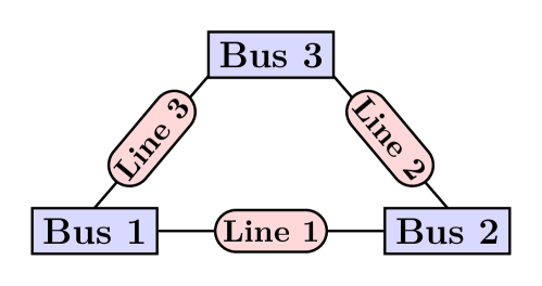
Figure 4: Simplified representation of the microgrid considered.

The microgrid under consideration is composed of three buses as illustrated in Fig. 4, where each bus is composed of a controlled buck converter connected to a load. Under the common assumptions that an average model for the DC-DC converter dynamics can be used (resulting from Assumption 1) and that switching losses may be ignored, the dynamics of each bus are given by

$$\left\{\begin{matrix}&\diff{i_{j}(t)}{t}=\dfrac{1}{L_{j}}\left(-v_{B_{j}}(t)-R_{j}i_{j}(t)+u_{j}(t)\right)\\ &\diff{v_{B_{j}}(t)}{t}=\dfrac{1}{C_{j}}\left(i_{j}(t)-i_{\text{Load}_{j}}(t)+i_{B_{j}}(t)\right)\\ \end{matrix}\right.$$ (18)

where $i_{j}(t)$ is the bus internal current (the inductor current), $i_{B_{j}}(t)$ is the bus injection current from the network, $v_{B_{j}}(t)$ is the bus output voltage and $u_{j}(t)$ is the control input of the buck converter. $R_{j}$, $L_{j}$ and $C_{j}$ are bus filter resistance, inductance and capacitance respectively. The control input, $u_{j}(t)$, is determined by the local controller at the bus and is actuated via the duty ratio of the DC-DC converter, usually with the goal of regulating the output voltage and/or achieving load sharing between the various DC-DC converters in the network. In this example, it is given as the output of a double PI controller with the following model, where $x_{K_{j}}(t)$ is the controller state vector.

$$\left\{\begin{matrix}&\diff{x_{K_{j}}(t)}{t}=\begin{pmatrix}0&0\\ K_{I_{v_{j}}}&0\end{pmatrix}x_{K_{j}}(t)+\dots\\ &\hskip 42.67912pt\dots+\begin{pmatrix}1&0\\ K_{P_{v_{j}}}&-1\end{pmatrix}\begin{pmatrix}e_{v_{j}}(t)\\ i_{j}(t)\end{pmatrix}\\ &u_{j}(t)=\begin{pmatrix}K_{P_{i_{j}}}K_{I_{v_{j}}}&\leavevmode\nobreak\ \leavevmode\nobreak\ K_{I_{i_{j}}}\end{pmatrix}x_{K_{j}}(t)+\cdots\\ &\leavevmode\nobreak\ \leavevmode\nobreak\ \leavevmode\nobreak\ \leavevmode\nobreak\ \leavevmode\nobreak\ \leavevmode\nobreak\ \leavevmode\nobreak\ \leavevmode\nobreak\ \cdots+\begin{pmatrix}K_{P_{i_{j}}}K_{P_{v_{j}}}&-K_{P_{i_{j}}}\end{pmatrix}\begin{pmatrix}e_{v_{j}}(t)\\ i_{j}(t)\end{pmatrix}\end{matrix}\right.$$ (19)

The gains $K_{P_{v_{j}}}$ and $K_{I_{v_{j}}}$ are the proportional and the integral gains, respectively, of the voltage PI controller (outer controller) while $K_{P_{i_{j}}}$ and $K_{I_{i_{j}}}$ are those of the current PI controller (inner controller). The signal $e_{v_{j}}(t)$ is the voltage tracking error given by $e_{v_{j}}(t)=v_{r_{j}}(t)-v_{B_{j}}(t)$ where $v_{r_{j}}(t)$ is the desired bus output voltage which is adjusted according to $i_{B_{j}}(t)$ such that $v_{r_{j}}(t)=v_{r_{\text{nom}}}+R_{\text{droop}_{j}}i_{B_{j}}(t)$ with $v_{r_{\text{nom}}}$ the nominal voltage and $R_{\text{droop}_{j}}$ the droop coefficient.

Note that the state vector $x_{B_{j}}(t)$ in (3) is in this case $x_{B_{j}}(t)=\begin{pmatrix}i_{j}(t)&v_{B_{j}}(t)&x_{K_{j}}^{\top}(t)\end{pmatrix}^{\top}$ while $f_{B_{j}}(x_{B_{j}}(t),i_{B_{j}}(t))$ is obtained by considering the right-hand side of the differential equations in (18)-(19) after replacing $u_{j}(t)$, $e_{v_{j}}(t)$, $v_{r_{j}}(t)$ and $i_{\text{Load}_{j}}(t)$ with their expressions given above. Note that the current $i_{\text{Load}_{j}}(t)$ in (18) is the load current and its expression depends on the load type as it will be shown in the two cases below.

IV-A Microgrid with resistive loads

In this case, each bus is connected to a resistive load $R_{\text{Load}_{j}}>0$ and $i_{\text{Load}_{j}}(t)$ is given by

$$i_{\text{Load}_{j}}(t)=R^{-1}_{\text{Load}_{j}}v_{B_{j}}(t).$$

To investigate the stability of this microgrid, we start with the usual passivity argument of Statement 1 corresponding to ${B_{j}(\mathbf{j}\omega)\in\mbox{$\bf{QC}$}(\Pi^{B_{j}}_{1},\epsilon_{B_{j}}(\omega))}$. The analysis reveals that the different buses are not passive over all frequencies especially at high frequencies as it can be seen in Fig. 5(a).

A common approach to enhance bus passivity is to increase the droop coefficients $R_{\text{droop}_{j}}$ until we have ${B_{j}(\mathbf{j}\omega)\in\mbox{$\bf{QC}$}(\Pi^{B_{j}}_{1},\epsilon_{B_{j}}(\omega))}$ at all frequencies. However, the consequence will be an important output voltage deviation from the nominal value $v_{r_{\text{nom}}}$ which makes this approach non practical for the operation of the microgrid.

To go beyond the passivity condition using Statement 1, we investigate if the small-gain condition ${B_{j}(\mathbf{j}\omega)\in\mbox{$\bf{QC}$}(\Pi^{B_{j}}_{2}(\mathbf{j}\omega),\epsilon_{B_{j}}(\omega))}$ is satisfied at least at high frequencies. The results presented in Fig. 5(b) affirm that the latter condition is satisfied at high frequencies where passivity failed. Hence, the microgrid of Fig. 4 with resistive loads is stable since Statement 1 is always satisfied at each frequency ${\omega\in\overline{\mathbf{R}}_{+}}$ as it can be seen in Fig. 5(c).

Therefore, a scalable control protocol when considering such microgrids in a general network topology can be to require the dynamics at each bus to satisfy

• ${B_{j}(\mathbf{j}\omega)\in\mbox{$\bf{QC}$}(\Pi^{B_{j}}_{1},\epsilon_{B_{j}}(\omega))}$ at a prescribed low frequency range $\omega<\omega_{c}$.

• ${B_{j}(\mathbf{j}\omega)\in\mbox{$\bf{QC}$}(\Pi^{B_{j}}_{2}(\mathbf{j}\omega),\epsilon_{B_{j}}(\omega))}$ at higher frequencies $\omega\geq\omega_{c}$.

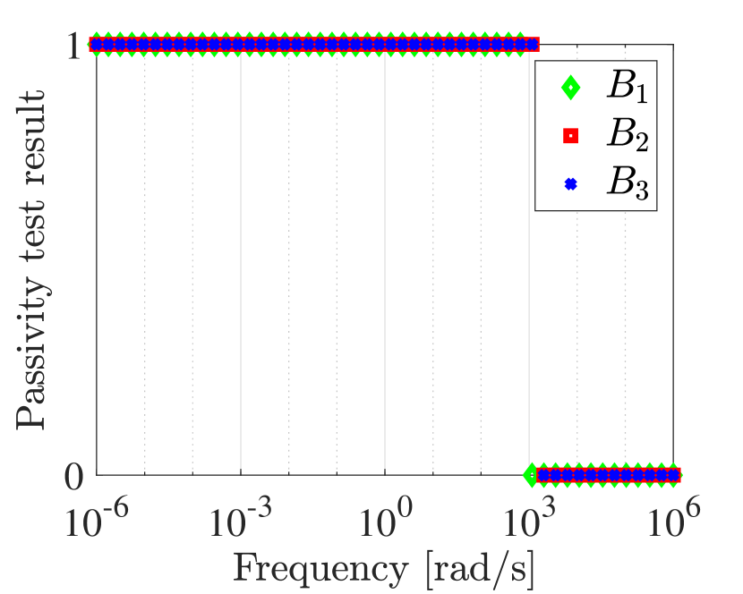
(a)

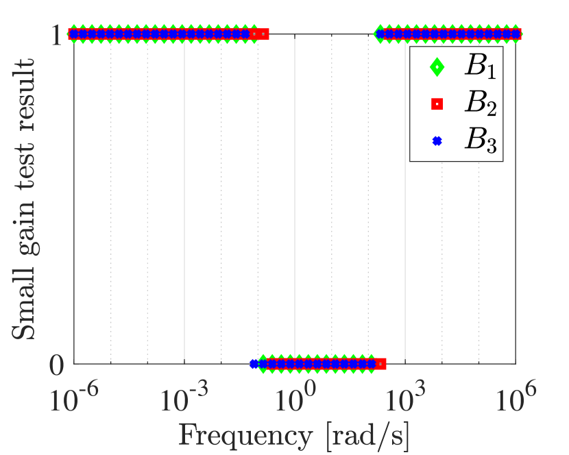
(b)

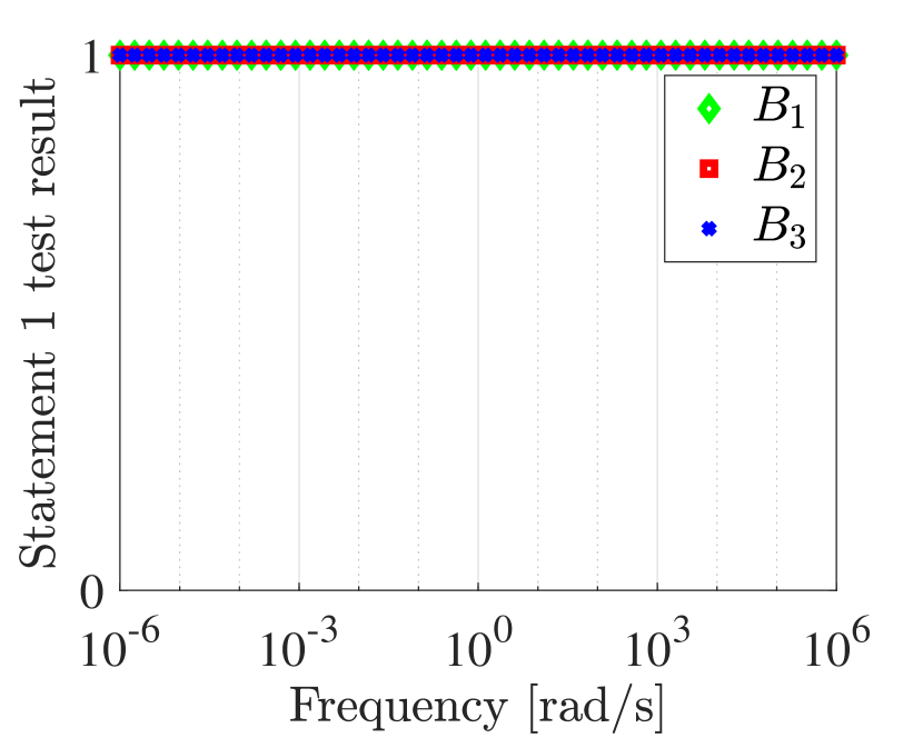
(c)

Figure 5: Stability assessment results of the microgrid of Fig. 4 with resistive loads using: (a) passivity, (b) small gain and (c) Statement 1 (passivity and small gain). Note that at each frequency, a value at 0 on the vertical axis means that the considered test has failed while 1 means it has passed.

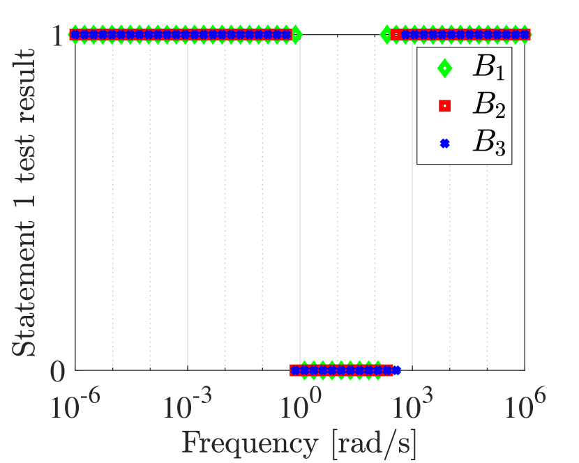
(a)

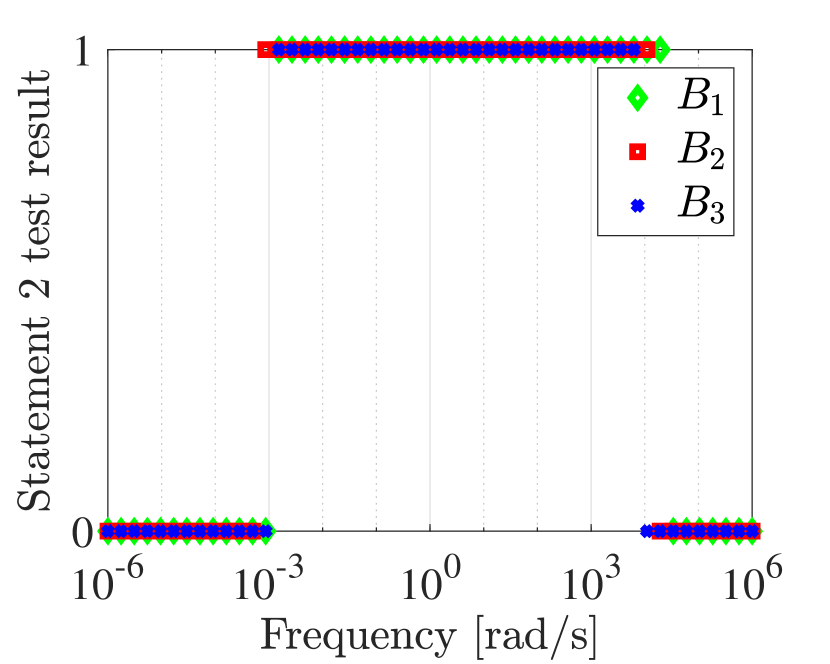
(b)

(c)

Figure 6: Stability assessment results of the microgrid of Fig. 4 with ZIP loads where $P_{\text{Load}_{j}}v_{r_{j}}^{-1}(t)>Z^{-1}_{\text{Load}_{j}}v_{r_{j}}(t)$ using: (a) Statement 1, (b) Statement 2 and (c) Theorem 1. Again note that at each frequency, a value at 0 on the vertical axis means that the considered test has failed while 1 means it has passed.

IV-B Microgrid with ZIP loads

We consider now the case where the loads are not just resistive and they also contain constant current and constant power elements. The load current $i_{\text{Load}_{j}}(t)$ becomes

$$i_{\text{Load}_{j}}(t)=\overline{i}_{\text{Load}_{j}}+Z^{-1}_{\text{Load}_{j}}v_{B_{j}}(t)+P_{\text{Load}_{j}}v^{-1}_{B_{j}}(t)$$

where $\overline{i}_{\text{Load}_{j}}$, $Z_{\text{Load}_{j}}=R_{\text{Load}_{j}}>0$ and $P_{\text{Load}_{j}}>0$ are the current, impedance and power of the constant current load, the constant impedance load and the constant power load respectively.

The presence of constant power loads has a destabilizing effect on the bus dynamics since they behave as negative resistance elements. To guarantee bus stability using a passivity argument, the effect of the constant impedance loads is larger than that of the constant power loads [15, 16], that is

$$Z^{-1}_{\text{Load}_{j}}v_{r_{j}}(t)>P_{\text{Load}_{j}}v_{r_{j}}^{-1}(t).$$

If the previous condition is satisfied, then it is possible to certify the stability of the microgrid with ZIP loads using Statement 1 in a similar way to the case of resistive loads presented earlier. Nevertheless, in many practical cases, the constant power loads can be larger than the constant impedance loads. In this case, Statement 1 alone will not be able to certify microgrid stability as it can be seen in Fig. 6(a). Note that in contrast to the case of resistive loads, the passivity condition does not hold at low frequencies while the small-gain condition holds. Note also that none of these conditions hold in medium frequencies, see Fig. 6(a).

Statement 2 allows to go beyond passivity and small-gain conditions of the conventional bus/line microgrid decomposition. In fact, the analysis reveals that by considering the small-gain condition in the new decomposition ${G_{j}(\mathbf{j}\omega)\in\mbox{$\bf{QC}$}(\Pi^{G_{j}}_{2},\epsilon_{G_{j}}(\omega))}$, Statement 2 is satisfied at medium frequencies where Statement 1 failed, see Fig. 6(b). Therefore, we have Statement 1 and/or Statement 2 satisfied at each frequency ${\omega\in\overline{\mathbf{R}}_{+}}$ as it can be seen in Fig. 6(c), and hence the microgrid of Fig. 4 with ZIP loads considered (dominated by constant power loads) is stable.

To conclude, when considering such microgrids in a general network topology, a scalable control protocol is to design controllers able to satisfy

• ${B_{j}(\mathbf{j}\omega)\in\mbox{$\bf{QC}$}(\Pi^{B_{j}}_{2}(\mathbf{j}\omega),\epsilon_{B_{j}}(\omega))}$ in a prescribed low frequency range.

• ${G_{j}(\mathbf{j}\omega)\in\mbox{$\bf{QC}$}(\Pi^{G_{j}}_{2},\epsilon_{G_{j}}(\omega))}$ in a prescribed medium frequency range.

• ${B_{j}(\mathbf{j}\omega)\in\mbox{$\bf{QC}$}(\Pi^{B_{j}}_{1},\epsilon_{B_{j}}(\omega))}$ at high frequencies.

Remark 6 (Post-analysis verification).

The analysis presented in Sections IV-A and IV-B has been carried out for a predefined set of individual frequencies. This analysis provides the frequency ranges and the corresponding conditions, which define the protocol that provides stability guarantees. Once this step is completed, we have used the generalized KYP lemma [23] as a post-analysis verification tool to effectively verify that the results obtained hold over the whole prescribed frequency ranges.

V Conclusions

We have derived decentralized stability conditions for DC microgrids. Our analysis takes into account the line dynamics and also allows higher order models for the DC-DC converters at each bus. By exploiting various decompositions of the network, we have derived multiple decentralized input-output stability conditions that also allow to exploit the coupling of each bus with neighboring lines. We have used appropriate homotopy arguments to combine these conditions pointwise over frequency thus reducing the conservatism in the analysis. The applicability of the obtained results has been illustrated through examples.

Appendix A Proof of Theorem 1

The following lemma is used in the proof of Theorem 1. It gives sufficient conditions that ensure that the point -1 is not included in the eigenloci of the return-ratio of the negative feedback interconnection of two stable linear systems.

Lemma 1.

Consider a negative feedback interconnection of $S_{1}\in\mathbb{RH}_{\infty}^{m\times n}$ and $S_{2}\in\mathbb{RH}_{\infty}^{n\times m}$. The point -1 is not included in the eigenloci of the return-ratio $S_{2}(s)S_{1}(s)$ when evaluated on the imaginary axis $\mathbf{j}\overline{\mathbf{R}}$, that is $-1\notin\lambda_{i}\left(S_{1}(\mathbf{j}\omega)S_{2}(\mathbf{j}\omega)\right)$ with $\omega\in\overline{\mathbf{R}}$, if there exists a scalar $\epsilon^{\Pi}(w)>0$ and a matrix $\Pi=\begin{pmatrix}\Pi_{11}&\Pi_{12}\\ \Pi_{12}^{*}&\Pi_{22}\end{pmatrix}$, where $\Pi_{11}:\mathbf{j}\overline{\mathbf{R}}\rightarrow\mathbf{C}^{m\times m}$, ${\Pi_{12}}:\mathbf{j}\overline{\mathbf{R}}\rightarrow\mathbf{C}^{m\times n}$ and $\Pi_{22}:\mathbf{j}\overline{\mathbf{R}}\rightarrow\mathbf{C}^{n\times n}$ such that for every $\omega\in\overline{\mathbf{R}}_{+}$, the following conditions hold

$$S_{1}(\mathbf{j}\omega)\in\mbox{$\bf{QC}$}\left(\Pi(\mathbf{j}\omega),\epsilon^{\Pi}(\omega)\right)$$ (20)

and

$$S_{2}(\mathbf{j}\omega)\in\mbox{$\overline{\bf{QC}}$}\left(\Pi(\mathbf{j}\omega),0\right).$$ (21)

Proof.

Suppose that $-1\in\lambda_{i}\left(S_{1}(\mathbf{j}\omega)S_{2}(\mathbf{j}\omega)\right)$ which means that $\left(I+S_{1}(\mathbf{j}\omega)S_{2}(\mathbf{j}\omega)\right)$ is not invertible, then there exists a non zero vector $w(\mathbf{j}\omega)\in\mathbb{C}^{m}$ different from zero such that $(I+S_{1}(\mathbf{j}\omega)S_{2}(\mathbf{j}\omega))w(\mathbf{j}\omega)=0.$ Letting $z(\mathbf{j}\omega)=-S_{2}(\mathbf{j}\omega)w(\mathbf{j}\omega)$, the previous equality becomes $w(\mathbf{j}\omega)-S_{1}(\mathbf{j}\omega)z(\mathbf{j}\omega)=0$ and we obtain $w(\mathbf{j}\omega)=S_{1}(\mathbf{j}\omega)z(\mathbf{j}\omega)$ together with $z(\mathbf{j}\omega)=-S_{2}(\mathbf{j}\omega)w(\mathbf{j}\omega)$. Let $\sigma(\mathbf{j}\omega)=\begin{pmatrix}w(\mathbf{j}\omega)^{*}\leavevmode\nobreak\ \leavevmode\nobreak\ z(\mathbf{j}\omega)^{*}\end{pmatrix}^{*}$. After pre and post multiplying the expanded forms (expanded as in (1)) of conditions (20) and (21) by $z(\mathbf{j}\omega)$ and $w(\mathbf{j}\omega)$ respectively, we obtain $\sigma(\mathbf{j}\omega)^{*}\Pi(\mathbf{j}\omega)\sigma(\mathbf{j}\omega)\geq{\color[rgb]{0,0,0}\epsilon^{\Pi}(\omega)}\leavevmode\nobreak\ w(\mathbf{j}\omega)^{*}w(\mathbf{j}\omega)$ and $\sigma(\mathbf{j}\omega)^{*}\Pi(\mathbf{j}\omega)\sigma(\mathbf{j}\omega)\leq 0$ which is a contradiction. Therefore, if conditions (20) and (21) are satisfied then $-1\notin\lambda_{i}\left(S_{1}(\mathbf{j}\omega)S_{2}(\mathbf{j}\omega)\right)$ for all $\omega\in\overline{\mathbf{R}}_{+}$. Due to the symmetry of $\lambda_{i}(S_{1}(\mathbf{j}\omega)S_{2}(\mathbf{j}\omega)))$ about the real axis, $-1\notin\lambda_{i}\left(S_{1}(\mathbf{j}\omega)S_{2}(\mathbf{j}\omega)\right)$ also holds for all $\omega\in\overline{\mathbf{R}}$. $\hfill\blacksquare$

The local asymptotic stability of the equilibrium (4) of the DC microgrid (2)-(3) is investigated via the internal stability [29, Def 5.2] of interconnection (5) [29, Lem 5.3], [30, Thm 3.7]. In particular, it is sufficient to show that the closed-loop transfer functions of interconnection (5) (as defined in [29, Lem 5.3]) have no poles in the closed right half-plane $\overline{\mathbf{C}}_{+}$. Therefore, as $B(s)$ and $L(s)$ have no poles in $\overline{\mathbf{C}}_{+}$, we only have to show that $(I+Q_{O}(s))^{-1}$ has no poles in $\overline{\mathbf{C}}_{+}$ with $Q_{O}(s)$ being the return-ratio of interconnection (5) given by

$$Q_{{O}}(s)=B(s)\mathcal{A}L(s)\mathcal{A}^{\top}.$$ (22)

Using ideas from [21, 22], interconnection (5) can also be represented equivalently as an interconnection of two systems $G(s)$ and $A$ such that

$$\left\{\begin{matrix}&Y(s)&=&\leavevmode\nobreak\ G(s)\leavevmode\nobreak\ X(s)\\ &X(s)&=&-A\leavevmode\nobreak\ \leavevmode\nobreak\ \leavevmode\nobreak\ Y(s)\end{matrix}\right.$$ (23)

where $G(s)=\oplus_{j=1}^{n_{b}}G_{j}(s)$ with

$$G_{j}(s)=L(s)\leavevmode\nobreak\ (a^{r}_{j})^{\top}\leavevmode\nobreak\ B_{j}(s)\leavevmode\nobreak\ a^{r}_{j}\leavevmode\nobreak\ \vspace{-0.3cm}$$ (24)

and

$$A=MM^{*}\vspace{-0.1cm}$$ (25)

with $M=\big{(}M_{1}^{*}\leavevmode\nobreak\ \dots\leavevmode\nobreak\ M_{n_{b}}^{*}\big{)}^{*}$ where

$$M_{j}=\oplus_{k=1}^{n_{\ell}}\Big{(}r^{j}_{k}\Big{)}\leavevmode\nobreak\ \leavevmode\nobreak\ \leavevmode\nobreak\ \leavevmode\nobreak\ \leavevmode\nobreak\ r^{j}_{k}=\left\{\begin{matrix}1\leavevmode\nobreak\ \leavevmode\nobreak\ \leavevmode\nobreak\ \leavevmode\nobreak\ \leavevmode\nobreak\ \text{if $\mathcal{A}_{jk}\neq 0$ }\\ 0\leavevmode\nobreak\ \leavevmode\nobreak\ \leavevmode\nobreak\ \leavevmode\nobreak\ \leavevmode\nobreak\ \text{otherwise}\leavevmode\nobreak\ \leavevmode\nobreak\ \leavevmode\nobreak\ \end{matrix}\right.\leavevmode\nobreak\ \leavevmode\nobreak\$$ (26)

We define the return-ratio of interconnection (23) as

$$Q_{N}(s)=G(s)MM^{*}.$$ (27)

The proof of Theorem 1 uses the quadratic graph separation arguments of Lemma 21, analogous to an IQC analysis, on representations (5) and (23), together with a homotopy argument, with stability deduced using the multivariable Nyquist criterion [31]. In particular, a main feature of the proof is that it allows to combine pointwise over frequency various decentralized conditions associated with the two different network decompositions (5), (23).
The proof consists of four parts. In Part 1, we show that if Statement 1 is true for each ${\omega\in\overline{\mathbf{R}}_{+}}$, then the point -1 is not included in the eigenloci of $Q_{{O}}(s)$ in (22). In Part 2, we show in the same way that if Statement 2 is true for each ${\omega\in\overline{\mathbf{R}}_{+}}$, then the point -1 is not included in the eigenloci of $Q_{{N}}(s)$ in (27). In Part 3, we show that if the point -1 is not included in the eigenloci of (27) then it is not included in the eigenloci $Q_{O}(s)$ of (22). Finally, we deduce in Part 4 using homotopy arguments that if at each frequency either Statement 1 or Statement 2 is true, then interconnection (5) is stable.
$\bullet$ Part 1: In this part, we demonstrate that having Statement 1 satisfied at each $\omega\in\overline{\mathbf{R}}_{+}$ is sufficient for conditions (20) and (21) in Lemma 21 to hold. This is done by exploiting the following two properties of interconnection (5).

1. Passivity of the power lines: From (2), it can be deduced that the line dynamics are passive which can be expressed in the frequency domain at each frequency $\omega\in\overline{\mathbf{R}}_{+}$ as $L_{k}(\mathbf{j}\omega)\in\mbox{$\overline{\bf{QC}}$}\left(\Pi^{B_{j}}_{1},0\right)$ with $\Pi^{B_{j}}_{1}$ given by (8). This is equivalent to

   $$\mathcal{A}L(\mathbf{j}\omega)\mathcal{A}^{\top}\in\mbox{$\overline{\bf{QC}}$}\left(\Pi^{B}_{1},0\right)$$ (28)

   with $\Pi^{B}_{1}=I_{n_{b}}\otimes\Pi^{B_{j}}_{1}$.
   

2. Bounding the power line induced $\infty$-norm: The induced $\infty$-norm of $\Xi(\mathbf{j}\omega)=\mathcal{A}L(\mathbf{j}\omega)\mathcal{A}^{\top}$ is given by $\max_{j}\left(|\sum_{k:k\in\mathcal{E}_{j}}L_{k}(\mathbf{j}\omega)|+\sum_{k:k\in\mathcal{E}_{j}}\left|L_{k}(\mathbf{j}\omega)\right|\right)$. To have a bound on this norm, we consider a scaling by the matrix $J_{B}(\mathbf{j}\omega)^{-1}=\left(\oplus_{j=1}^{n_{b}}{J_{B_{j}}}(\mathbf{j}\omega)\right)^{-1}$, where $J_{B_{j}}(\mathbf{j}\omega)$ is given by (10). In particular, $\left\|J_{B}(\mathbf{j}\omega)^{-1}\Xi(\mathbf{j}\omega)\right\|_{\infty}$ is given by

   $$\max_{j}J_{B_{j}}(\mathbf{j}\omega)^{-1}\Big{(}|\sum_{k:k\in\mathcal{E}_{j}}L_{k}(\mathbf{j}\omega)|+\sum_{k:k\in\mathcal{E}_{j}}|L_{k}(\mathbf{j}\omega)|\Big{)}$$

   which is equal to 1. Furthermore, we also have $\left\|J_{B}(\mathbf{j}\omega)^{-1}\Xi(\mathbf{j}\omega)^{*}\right\|_{\infty}=1$. Now, let $F(\mathbf{j}\omega)=J_{B}(\mathbf{j}\omega)^{-1}\Xi(\mathbf{j}\omega)^{*}J_{B}(\mathbf{j}\omega)^{-1}\Xi(\mathbf{j}\omega)$. The spectral radius of $F(\mathbf{j}\omega)$ can be bounded using the induced $\infty$-norm as follows

   $$\rho(F(\mathbf{j}\omega)) \leq\left\|F(\mathbf{j}\omega)\right\|_{\infty}$$

   $$\leq\left\|J_{B}(\mathbf{j}\omega)^{-1}\Xi(\mathbf{j}\omega)^{*}\right\|_{\infty}\left\|J_{B}(\mathbf{j}\omega)^{-1}\Xi(\mathbf{j}\omega)\right\|_{\infty}$$

   $$\leq 1$$ (29)

   We now note that $F(\mathbf{j}\omega)$ has real eigenvalues as it is the product of a positive definite and a Hermitian matrix. Therefore, since from (29) $\rho(F(\mathbf{j}\omega))\leq 1$, the eigenvalues of $J_{B}(\mathbf{j}\omega)^{-1}(\mathcal{A}L(\mathbf{j}\omega)\mathcal{A}^{\top})^{*}J_{B}(\mathbf{j}\omega)^{-1}\mathcal{A}L(\mathbf{j}\omega)\mathcal{A}^{\top}-I_{n_{b}}$ are less than or equal to zero. Moreover, as $J_{B}(\mathbf{j}\omega)$ is positive definite, the eigenvalues of $(\mathcal{A}L(\mathbf{j}\omega)\mathcal{A}^{\top})^{*}J_{B}(\mathbf{j}\omega)^{-1}\mathcal{A}L(\mathbf{j}\omega)\mathcal{A}^{\top}-J_{B}(\mathbf{j}\omega)$ are also less than or equal to zero leading to

   $$(\mathcal{A}L(\mathbf{j}\omega)\mathcal{A}^{\top})^{*}J_{B}(\mathbf{j}\omega)^{-1}\mathcal{A}L(\mathbf{j}\omega)\mathcal{A}^{\top}\leq J_{B}(\mathbf{j}\omega)$$

   which can be written in compact form as

   $$\mathcal{A}L(\mathbf{j}\omega)\mathcal{A}^{\top}\in\mbox{$\overline{\bf{QC}}$}\left(\Pi^{B}_{2}(\mathbf{j}\omega),0\right)$$ (30)

   with $\Pi^{B}_{2}(\mathbf{j}\omega)=\begin{pmatrix}-J_{B}(\mathbf{j}\omega)&0\\ 0&J_{B}(\mathbf{j}\omega)^{-1}\end{pmatrix}.$

As $\mathcal{A}L(\mathbf{j}\omega)\mathcal{A}^{\top}$ satisfies (28) and (30), it will satisfy

$$\mathcal{A}L(\mathbf{j}\omega)\mathcal{A}^{\top}\in\mbox{$\overline{\bf{QC}}$}\left(\gamma_{1}(\omega)\Pi^{B}_{1}+\gamma_{2}(\omega)\Pi^{B}_{2}(\mathbf{j}\omega),0\right)$$

with $\gamma_{1}(\omega)\geq 0$ and $\gamma_{2}(\omega)\geq 0$. Moreover, to exploit the diagonal structure of $\Pi^{B}_{1}$ and $\Pi^{B}_{2}(\mathbf{j}\omega)$, the scalars $\gamma_{1}(\omega)$ and $\gamma_{2}(\omega)$ can be replaced by two diagonal matrices $\Gamma_{1}(\omega)=I_{2}\otimes\left(\oplus_{j=1}^{n_{b}}\gamma_{j1}(\omega)\right)$ and $\Gamma_{2}(\omega)=I_{2}\otimes\left(\oplus_{j=1}^{n_{b}}\gamma_{j2}(\omega)\right)$, with $\gamma_{j1}(\omega)\geq 0$ and $\gamma_{j2}(\omega)\geq 0$ associated to $\Pi^{B_{j}}_{1}$ and $\Pi^{B_{j}}_{2}(\mathbf{j}\omega)$ respectively. We can thus write

$$\mathcal{A}L(\mathbf{j}\omega)\mathcal{A}^{\top}\in\mbox{$\overline{\bf{QC}}$}\left(\Gamma_{1}(\omega)\Pi^{B}_{1}+\Gamma_{2}(\omega)\Pi^{B}_{2}(\mathbf{j}\omega),0\right)$$ (31)

Therefore, for (20) and (21) of Lemma 21 to hold it is sufficient at each $\omega\in\overline{\mathbf{R}}_{+}$ to find a scalar $\epsilon_{B}(\omega)>0$ such that

$${\color[rgb]{0,0,0}\oplus_{j=1}^{n_{b}}B_{j}(\mathbf{j}\omega)\in\mbox{$\bf{QC}$}\left(\Gamma_{1}(\omega)\Pi^{B}_{1}+\Gamma_{2}(\omega)\Pi^{B}_{2}(\mathbf{j}\omega),\epsilon_{B}(\omega)\right)}.$$

Due to the diagonal structure of $\Gamma_{1}(\omega)\Pi^{B}_{1}+\Gamma_{2}(\omega)\Pi^{B}_{2}(\mathbf{j}\omega)$, the previous condition can be decomposed into $n_{b}$ conditions given by (7) with $\epsilon_{B_{j}}(\omega)\geq\epsilon_{B}(\omega){>0}$.
Hence if Statement 1 holds for each $\omega\in\overline{\mathbf{R}}_{+}$ then (20) and (21) hold, and it therefore follows from Lemma 21 that the point -1 is not included in the eigenloci of the return-ratio $Q_{O}(s)$ of interconnection (5) given by (22).
$\bullet$ Part 2: Similarly to Part 1, we prove that if Statement 2 is satisfied at each $\omega\in\overline{\mathbf{R}}_{+}$ then it is sufficient for (20) and (21) of Lemma 21 to hold. This is done by exploiting the following properties and structure of interconnection (23).

1. Positivity and symmetry of $A$: As $A=MM^{*}\geq 0$ and $A=A^{*}$, we have $-A^{*}-A\leq 0$ which rewrites in its compact form as

   $$A\in\mbox{$\overline{\bf{QC}}$}\left(\Pi^{G}_{1},0\right)$$ (32)

   where $\Pi^{G}_{1}=I_{n_{b}}\otimes\Pi^{G_{j}}_{1}$ with $\Pi^{G_{j}}_{1}$ given by (12).
   

2. Bounding the induced $\infty$-norm of $A$: Using (25) and (26), the induced $\infty$-norm of $A$ defined as the maximum row sum $r_{k}^{j}\sum_{j=1}^{n_{b}}r^{j}_{k}$ is always equal to 2 since $\sum_{j=1}^{n_{b}}r^{j}_{k}=2$ as the graph associated with the microgrid is connected. Therefore, $\left\|A\right\|_{\infty}=2$ and since $\rho(A)\leq\left\|A\right\|_{\infty}$ with $A$ symmetric, we obtain $A^{*}A\leq 4I_{n_{b}n_{\ell}}$ which can be written in compact form as

   $$A\in\mbox{$\overline{\bf{QC}}$}\left(\Pi^{G}_{2},0\right)$$ (33)

   where $\Pi^{G}_{2}=I_{n_{b}}\otimes\Pi^{G_{j}}_{2}$ with $\Pi^{G_{j}}_{2}$ given by (13).
   

3. Exploiting the structure of $A$: To take into account the fact that the lines are part of the new subsystems $G_{j}$, we use $\Pi^{G}_{3}(\mathbf{j}\omega)=I_{n_{b}}\otimes\Pi^{G_{j}}_{3}(\mathbf{j}\omega)$ with $\Pi^{G_{j}}_{3}(\mathbf{j}\omega)$ given by (14). With this particular choice of $\Pi^{G}_{3}(\mathbf{j}\omega)$, we can associate each $\Pi^{k}(\mathbf{j}\omega)$ to each line $L_{k}(\mathbf{j}\omega)$. Note that if $-\Pi^{k}_{12}(\mathbf{j}\omega)-\Pi^{k}_{12}(\mathbf{j}\omega)^{*}+2\leavevmode\nobreak\ \Pi^{k}_{22}(\mathbf{j}\omega)\leq 0$ together with $\Pi^{k}_{11}(\mathbf{j}\omega)\leq 0$ then

   $$A\in\mbox{$\overline{\bf{QC}}$}\left(\Pi^{G}_{3}(\mathbf{j}\omega),0\right)$$ (34)

   is always satisfied. To see this, note that by exploiting the sparsity of $A$ and the structure of $\Pi^{G}_{3}(\mathbf{j}\omega)$, the left hand side of the expanded form of the condition in (34) is given by

   $$\begin{matrix}I_{n_{b}}\otimes(\oplus_{k=1}^{n_{\ell}}\Pi^{k}_{11}(\mathbf{j}\omega))+\cdots\\ \cdots+MM^{*}(I_{n_{b}}\otimes(\oplus_{k=1}^{n_{\ell}}\Pi^{k}_{22}(\mathbf{j}\omega)))MM^{*}-\cdots\\ \cdots-M(\oplus_{k=1}^{n_{\ell}}\Pi^{k}_{12}(\mathbf{j}\omega))M^{*}-M(\oplus_{k=1}^{n_{\ell}}\Pi^{k}_{12}(\mathbf{j}\omega)^{*})M^{*}\end{matrix}$$

   which is equal to

   $$\begin{matrix}&I_{n_{b}}\otimes(\oplus_{k=1}^{n_{\ell}}\Pi^{k}_{11}(\mathbf{j}\omega))+\cdots\\ &\cdots+M\big{(}\oplus_{k=1}^{n_{\ell}}\big{(}-\Pi^{k}_{12}(\mathbf{j}\omega)-\Pi^{k}_{12}(\mathbf{j}\omega)^{*}+\cdots\\ &\leavevmode\nobreak\ \leavevmode\nobreak\ \leavevmode\nobreak\ \leavevmode\nobreak\ \leavevmode\nobreak\ \leavevmode\nobreak\ \leavevmode\nobreak\ \leavevmode\nobreak\ \leavevmode\nobreak\ \leavevmode\nobreak\ \leavevmode\nobreak\ \leavevmode\nobreak\ \cdots+2\Pi^{k}_{22}(\mathbf{j}\omega)\big{)}\big{)}M^{*}.\end{matrix}$$ (35)

   Hence $\Pi^{k}_{11}(\mathbf{j}\omega)\leq 0$ together with $-\Pi^{k}_{12}(\mathbf{j}\omega)-\Pi^{k}_{12}(\mathbf{j}\omega)^{*}+2\Pi^{k}_{22}(\mathbf{j}\omega)\leq 0$ are sufficient for (35) to be negative semi-definite and hence for condition (34) to hold.

Therefore, as $A$ satisfies (32), (33) and (34) and using similar arguments to those in Part 1, we obtain

$$\begin{matrix}A\in\mbox{$\overline{\bf{QC}}$}\left(\Delta_{1}(\omega)\Pi^{G}_{1}+\Delta_{2}(\omega)\Pi^{G}_{2}+\cdots\leavevmode\nobreak\ \leavevmode\nobreak\ \leavevmode\nobreak\ \leavevmode\nobreak\ \right.\\ \cdots+\left.\Delta_{3}(\omega)\Pi^{G}_{3}(\mathbf{j}\omega),\epsilon_{G}(\omega)\right)\end{matrix}$$ (36)

where $\Delta_{i}(\omega)=I_{2n_{\ell}}\otimes\left(\oplus_{j=1}^{n_{b}}\delta_{ji}(\omega)\right)$ with $i\in\{1,2,3\}$, and $\delta_{ji}(\omega)\geq 0$. Therefore, for (20) and (21) in Lemma 21 to hold it is sufficient at each $\omega\in\overline{\mathbf{R}}_{+}$ to find a scalar $\epsilon_{G}(\omega)>0$ such that

$$\begin{matrix}\oplus_{j=1}^{n_{b}}G_{j}(\mathbf{j}\omega)\in\mbox{$\bf{QC}$}\left(\Delta_{1}(\omega)\Pi^{G}_{1}+\Delta_{2}(\omega)\Pi^{G}_{2}+\cdots\leavevmode\nobreak\ \leavevmode\nobreak\ \leavevmode\nobreak\ \leavevmode\nobreak\ \right.\\ \cdots+\left.\Delta_{3}(\omega)\Pi^{G}_{3}(\mathbf{j}\omega),\epsilon_{G}(\omega)\right).\end{matrix}$$

Due to the diagonal structure of $\Delta_{i}$ and $\Pi^{G}_{i}$, the previous condition can be decomposed into $n_{b}$ conditions given by (11) with $\epsilon_{G_{j}}(\omega)\geq\epsilon_{G}(\omega){>0}$.
Hence if Statement 2 holds for each $\omega\in\overline{\mathbf{R}}_{+}$ then (20) and  (21) hold, and it therefore follows from Lemma 21 that the point -1 is not included in the eigenloci of the return-ratio $Q_{N}(s)$ of interconnection (23) given by (27).
$\bullet$ Part 3: We show in this part that if the point -1 is not included in the eigenloci of $Q_{N}(s)$ in (27), then it is also not included in the eigenloci of $Q_{O}(s)$ in (22). A simple argument shows that both return-ratios have the same non-zero eigenvalues. In particular, the matrix $G(s)MM^{*}$ in $Q_{N}(s)$ has the same nonzero eigenvalues as $M^{*}G(s)M$ which rewrites as $\sum_{j=1}^{{\color[rgb]{0,0,0}n_{b}}}M_{j}G_{j}(s)M_{j}^{*}$. Then using the expressions of $G_{j}(s)$ and $M_{j}$ given by (24) and (26) and the fact that $L(s)M_{j}=M_{j}L(s)$, the previous summation becomes $L(s)\sum_{j=1}^{n_{b}}M_{j}(a^{r}_{j})^{\top}B_{j}(s)a^{r}_{j}M_{j}^{*}$ which rewrites as $L(s)\mathcal{A}^{\top}B(s)\mathcal{A}$. Finally, note that $L(s)\mathcal{A}^{\top}B(s)\mathcal{A}$ has the same nonzero eigenvalues as $B(s)\mathcal{A}L(s)\mathcal{A}^{\top}$ which is the return-ratio $Q_{O}(s)$. Hence, if the point -1 is not included in the eigenloci of the return-ratio $Q_{N}(s)$ of interconnection (23), then it is also not included in the eigenloci of the return-ratio $Q_{O}(s)$ of interconnection (5).
$\bullet$ Part 4: We show now using a homotopy argument that when at each frequency Statement 1 or Statement 2 is satisfied then the point $-1$ is also not encircled by the eigenloci of the return-ratio of (5) or (23), and hence stability can be deduced. We define the following linear homotopy for interconnection (5): $\mathcal{A}L_{\tau}(\mathbf{j}\omega)\mathcal{A}^{\top}=\mathcal{A}L(\mathbf{j}\omega)\mathcal{A}^{\top}$ and $B_{j,\tau}(\mathbf{j}\omega)=\tau B_{j}(\mathbf{j}\omega)$ with $\tau\in[0,1]$. Similarly, we define an analogous homotopy for the interconnection (23) as $A_{\tau}=A$ and $G_{j,\tau}(\mathbf{j}\omega)=\tau{G_{j}}(\mathbf{j}\omega)$ with the same $\tau\in[0,1]$. We will show that throughout these homotopies, condition (7) together with (31) and condition (11) together with (36) remain satisfied, i.e. when $B_{j}(\mathbf{j}\omega)$, $\mathcal{A}L(\mathbf{j}\omega)\mathcal{A}^{\top}$, $B_{j}(\mathbf{j}\omega)$ and $A$ and are replaced by $B_{j,\tau}(\mathbf{j}\omega)$, $\mathcal{A}L_{\tau}(\mathbf{j}\omega)\mathcal{A}^{\top}$, $G_{j,\tau}(\mathbf{j}\omega)$ and $A_{\tau}$ respectively.
Conditions (31) and (36) are always satisfied when $\gamma_{ji}(\omega)\geq 0$, $\delta_{ji}(\omega)\geq 0$, $J_{B_{j}}(\mathbf{j}\omega)$ is given by (10), $\Pi^{k}_{11}(\mathbf{j}\omega)\leq 0$, and $-\Pi^{k}_{12}(\mathbf{j}\omega)-\Pi^{k}_{12}(\mathbf{j}\omega)^{*}+2\Pi^{k}_{22}(\mathbf{j}\omega)\leq 0$.
On the other hand, conditions (7) and (11) rewrite in their expanded forms as $\Phi_{j}(\mathbf{j}\omega)\geq 0$ and $\Psi_{j}(\mathbf{j}\omega)\geq 0$ with $\Phi_{j}(\mathbf{j}\omega)$ and $\Psi_{j}(\mathbf{j}\omega)$ given by

$$\begin{matrix}&\Phi_{j}(\mathbf{j}\omega)=-\tau^{2}\epsilon_{B_{j}}(\omega)B_{j}(\mathbf{j}\omega)^{*}B_{j}(\mathbf{j}\omega)+\cdots\\ &\cdots+\begin{pmatrix}\tau B_{j}(\mathbf{j}\omega)\\ 1\end{pmatrix}^{*}\Big{(}\gamma_{j1}(\omega)\Pi^{B_{j}}_{1}+\cdots\\ &\leavevmode\nobreak\ \leavevmode\nobreak\ \leavevmode\nobreak\ \leavevmode\nobreak\ \leavevmode\nobreak\ \leavevmode\nobreak\ \leavevmode\nobreak\ \leavevmode\nobreak\ \leavevmode\nobreak\ \leavevmode\nobreak\ \leavevmode\nobreak\ \leavevmode\nobreak\ \cdots+\gamma_{j2}(\omega)\Pi^{B_{j}}_{2}(\mathbf{j}\omega)\Big{)}\begin{pmatrix}\tau B_{j}(\mathbf{j}\omega)\\ 1\end{pmatrix}\end{matrix}$$

and

$$\begin{matrix}&\Psi_{j}(\mathbf{j}\omega)=-\tau^{2}\epsilon_{G_{j}}(\omega)G_{j}(\mathbf{j}\omega)^{*}G_{j}(\mathbf{j}\omega)+\cdots\\ &\cdots+\begin{pmatrix}\tau G_{j}(\mathbf{j}\omega)\\ I\end{pmatrix}^{*}\Big{(}\delta_{j1}(\omega)\Pi^{G_{j}}_{1}+\cdots\\ &\leavevmode\nobreak\ \leavevmode\nobreak\ \leavevmode\nobreak\ \leavevmode\nobreak\ \leavevmode\nobreak\ \leavevmode\nobreak\ \leavevmode\nobreak\ \leavevmode\nobreak\ \leavevmode\nobreak\ \leavevmode\nobreak\ \leavevmode\nobreak\ \leavevmode\nobreak\ \cdots+\delta_{j2}(\omega)\Pi^{G_{j}}_{2}+\delta_{j3}(\omega)\Pi^{G_{j}}_{3}(\mathbf{j}\omega)\Big{)}\begin{pmatrix}\tau G_{j}(\mathbf{j}\omega)\\ I\end{pmatrix}\end{matrix}$$

For $\tau=1$, $\Phi_{j}(\mathbf{j}\omega)\geq 0$ and $\Psi_{j}(\mathbf{j}\omega)\geq 0$ are satisfied from Part 1 and Part 2.
For $\tau=0$, $\Phi_{j}(\mathbf{j}\omega)\geq 0$ and $\Psi_{j}(\mathbf{j}\omega)\geq 0$ are also satisfied as $\gamma_{j1}(\omega)\big{(}\Pi^{B_{j}}_{1}\big{)}_{22}+\gamma_{j2}(\omega)\big{(}\Pi^{B_{j}}_{2}(\mathbf{j}\omega)\big{)}_{22}\geq 0$   and    $\delta_{j1}(\omega)\big{(}\Pi^{G_{j}}_{1}\big{)}_{22}+\delta_{j2}(\omega)\big{(}\Pi^{G_{j}}_{2}\big{)}_{22}+\delta_{j3}(\omega)\big{(}\Pi^{G_{j}}_{i}(\mathbf{j}\omega)\big{)}_{22}\geq 0$ where $\big{(}\Pi^{B_{j}}_{i}\big{)}_{22}$ and $\big{(}\Pi^{G_{j}}_{3}\big{)}_{22}$ are the lower right blocks of $\Pi^{B_{j}}_{i}(\mathbf{j}\omega)$ and $\Pi^{G_{j}}_{i}(\mathbf{j}\omega)$ respectively.
For $\tau\in(0,1)$, $\Phi_{j}(\mathbf{j}\omega)\geq 0$ and $\Psi_{j}(\mathbf{j}\omega)\geq 0$ are also satisfied since $\Phi_{j}(\mathbf{j}\omega)$ and $\Psi_{j}(\mathbf{j}\omega)$ are concave in $\tau$ as $\gamma_{j1}(\omega)\big{(}\Pi^{B_{j}}_{1}\big{)}_{11}+\gamma_{j2}(\omega)\big{(}\Pi^{B_{j}}_{2}(\mathbf{j}\omega)\big{)}_{11}\leq 0$ and $\delta_{j1}(\omega)\big{(}\Pi^{G_{j}}_{1}\big{)}_{11}+\delta_{j2}(\omega)\big{(}\Pi^{G_{j}}_{2}\big{)}_{11}+\delta_{j3}(\omega)\big{(}\Pi^{G_{j}}_{3}(\mathbf{j}\omega)\big{)}_{11}\leq\leavevmode\nobreak\ 0$. Therefore, condition (7) together with (31) and condition (11) together with (36) remain satisfied when using the aforementioned homotopies, and hence the point -1 remains not included in the corresponding eigenloci of the return-ratio. Moreover, using the result of Part 3, if either Statement 1 or Statement 2 are satisfied at each frequency then the point $-1$ remains not included in the eigenloci of the return-ratio of interconnection (5) and hence the winding number of the point $-1$ does not change throughout the homotopies described above. Therefore, since the winding number is zero for $\tau=0$, it is also zero for $\tau=1$.

To summarize, if either Statement 1 or Statement 2 holds at each frequency ${\omega\in\overline{\mathbf{R}}_{+}}$ then the eigenloci of $B(\mathbf{j}\omega)\mathcal{A}L(\mathbf{j}\omega)\mathcal{A}^{\top}$ do not include the point -1 and do not encircle it. Hence, from the multivariable Nyquist criterion [31] it follows that the closed-loop transfer functions of interconnection (5) have no poles in $\overline{\mathbf{C}}_{+}$. Therefore, the equilibrium (4) of the power system (2)-(3) with its small-signal model (5) is locally asymptotically stable which concludes the proof of Theorem 1. $\hfill\blacksquare$

Appendix B Proof of Theorem 2

The proof is similar to the proof of Theorem 1, however the presence of an integrator introduces additional complications in the analysis that need to be explicitly addressed.

Consider the small-signal model (15) and consider the following decomposition of $L(s)$ and $\Theta_{L}(s)$

$$L(s)=\dfrac{1}{s}H(s)\leavevmode\nobreak\ \leavevmode\nobreak\ \leavevmode\nobreak\ \leavevmode\nobreak\ \leavevmode\nobreak\ \leavevmode\nobreak\ \leavevmode\nobreak\ \leavevmode\nobreak\ \leavevmode\nobreak\ \leavevmode\nobreak\ \Theta_{L}(s)=\dfrac{1}{s}\Theta_{H}(s).$$

The voltage and the current deviations $\overline{V_{B}}(s)$ and $\overline{I_{L}}(s)$ can be written in terms of the initial conditions $\overline{x_{B}}(0)$ and $\overline{x_{L}}(0)$ as

$$\begin{pmatrix}\overline{V_{B}}(s)\\ \overline{I_{L}}(s)\end{pmatrix}=\chi(s)\begin{pmatrix}\overline{x_{B}}(0)\\ \overline{x_{L}}(0)\end{pmatrix}$$ (37)

with

$$\begin{split}&\chi_{11}(s)=\left(I+B(s)\mathcal{A}s^{-1}H(s)\mathcal{A}^{\top}\right)^{-1}\Theta_{B}(s)\\ &\chi_{12}(s)=-\left(I+B(s)\mathcal{A}s^{-1}H(s)\mathcal{A}^{\top}\right)^{-1}B(s)\mathcal{A}\leavevmode\nobreak\ s^{-1}\Theta_{H}(s)\\ &\chi_{21}(s)=\left(I+s^{-1}H(s)\mathcal{A}^{\top}B(s)\mathcal{A}\right)^{-1}s^{-1}H(s)\mathcal{A}^{T}\leavevmode\nobreak\ \Theta_{B}(s)\\ &\chi_{22}(s)=\left(I+s^{-1}H(s)\mathcal{A}^{\top}B(s)\mathcal{A}\right)^{-1}s^{-1}\Theta_{H}(s)\end{split}$$

with $\Theta_{B}(s)$ given by (6) and $\Theta_{H}(s)=s\leavevmode\nobreak\ \Theta_{L}(s)$ with $\Theta_{L}(s)$ given by (16). Note that $B(s)$, $\Theta_{B}(s)$, $H(s)$ and $\Theta_{H}(s)$ have no poles in $\overline{\mathbf{C}}_{+}$ from Assumption 3 and Assumption 4.

The proof of Theorem 2 has two parts. We show in Part 1 that the function $\chi(s)$ has at most one pole at $s=0$ using ideas analogous to those in [32], and we show in Part 2 that $\chi(s)$ has no poles in the closed right half-plane excluding the origin i.e.  $\overline{\mathbf{C}}_{+}\setminus\{0\}$. These results are used to deduce the convergence of $\overline{v_{B}}(t)$ and $\overline{i_{L}}(t)$ to a constant value.
$\bullet$ Part 1: We show in this part that $\chi(s)$ in (37) has one simple pole at 0. This is done in two steps.

• Step 1: We show that $\left(I+B(s)\mathcal{A}s^{-1}H(s)\mathcal{A}^{\top}\right)^{-1}$ and $\left(I+s^{-1}H(s)\mathcal{A}^{\top}B(s)\mathcal{A}\right)^{-1}$ have no poles at $s=0$. To do this, we start by showing that $\left(I+B(s)\mathcal{A}s^{-1}H(s)\mathcal{A}^{\top}\right)$ has no zeros at $s=0$.
  Note that $s\left(I+B(s)\mathcal{A}s^{-1}H(s)\mathcal{A}^{\top}\right)$ is equal to $\left(sI+B(s)\mathcal{A}H(s)\mathcal{A}^{\top}\right)$. Since the underlying graph is connected then $\mathcal{A}H(\mathbf{j}0)\mathcal{A}^{\top}$ has a simple eigenvalue at the origin. Using the fact that $B(\mathbf{j}0)=\oplus_{j=1}^{n_{b}}B_{j}(\mathbf{j}0)>0$ (see Remark 5) we have that $s\left(I+B(s)\mathcal{A}s^{-1}H(s)\mathcal{A}^{\top}\right)$ has a simple zero at $s=0$, hence $\left(I+B(s)\mathcal{A}s^{-1}H(s)\mathcal{A}^{\top}\right)$ has no zeros at $s=0$ and $\left(I+B(s)\mathcal{A}s^{-1}H(s)\mathcal{A}^{\top}\right)^{-1}$ has no poles at $s=0$. The reasoning is the same to show that $\left(I+s^{-1}H(s)\mathcal{A}^{\top}B(s)\mathcal{A}\right)^{-1}$ has no poles at $s=0$.
  

• Step 2: We show in this step that $\chi_{12}(s)$ and $\chi_{21}(s)$ have no poles at $s=0$. For this purpose, we use the following limit from [33]: for a complex non-square matrix $\Lambda$, the limit $\lim_{s\rightarrow 0}(sI+\Lambda^{*}\Lambda)^{-1}\Lambda^{*}$ is equal to the pseudo-inverse of $\Lambda$. We start with $\lim_{s\rightarrow 0}\chi_{12}(s)$. We recall that $B(s)$, $H(s)$ and $\Theta_{H}(s)$ have no poles at $s=0$ and note that $H(\mathbf{j}0)>0$. Therefore, $\lim_{s\rightarrow 0}\chi_{12}(s)=\lim_{s\rightarrow 0}U(sI+V^{*}V)^{-1}V^{*}W^{-1}\Theta_{H}(\mathbf{j}0)$ with $U=\left(B(\mathbf{j}0)\right)^{\frac{1}{2}}$, $W=\left(H(\mathbf{j}0)\right)^{\frac{1}{2}}$ and $V^{*}=U\mathcal{A}W$; we thus see that $\chi_{12}(s)$ exists at $s=0$ and hence $\chi_{12}(s)$ has no poles at $s=0$. Using a similar argument, we can show that $\chi_{21}(s)$ has no poles at $s=0$.

Therefore, from the previous steps, we conclude that $\chi_{11}(s)$, $\chi_{12}(s)$ and $\chi_{21}(s)$ have no poles at $s=0$ while $\chi_{22}(s)$ has one simple pole at $s=0$ and hence the function $\chi(s)$ in (37) has one simple pole at $s=0$.

$\bullet$ Part 2: We show in this part that if at least one of the statements of Theorem 1 is satisfied for each ${\omega\in\overline{\mathbf{R}}_{+}\setminus\{0\}}$ and if $B_{j}(\mathbf{j}0)>0$, then $\chi(s)$ of (37) has no poles in $\overline{\mathbf{C}}_{+}\setminus\{0\}$. For this purpose, we adopt the notation below that is used to define a modified Nyquist contour.

• $C_{R}$, with $R>0$ sufficiently large, is the semi-circle centered at the origin of radius $R$ in the right-half plane, that is $C_{R}=\{s\in\mathbf{C}:\left|s\right|=R,\text{Re}(s)\geq 0\}$ where $\text{Re}(s)$ denotes the real part of $s$.

• $c_{r}(\mathbf{j}0)$, with $r>0$ sufficiently small, is the semi-circle centered at the origin of radius $r$ in the right-half plane, that is $c_{r}(\mathbf{j}0)=\{s\in\mathbf{C}:\left|s\right|=r,\text{Re}(s)>0\}$.

• $C_{\ell\setminus r}$ is the contour parameterized by $r$ defined by $C_{\ell\setminus r}=\mathbf{j}(-\infty,-r]\cup\mathbf{j}[+r,\infty)$ which is a straight line on the imaginary axis excluding the segment $\mathbf{j}(-r,+r)$.

The modified Nyquist contour is given by

$$C_{N}=C_{\ell\setminus r}\cup C_{R}\cup c_{r}(\mathbf{j}0).$$ (38)

As $B(s)\mathcal{A}s^{-1}H(s)\mathcal{A}^{\top}$ and $s^{-1}H(s)\mathcal{A}^{\top}B(s)\mathcal{A}$ have the same nonzero eigenvalues, $\left(I+B(s)\mathcal{A}s^{-1}H(s)\mathcal{A}^{\top}\right)^{-1}$ has the same poles as $\left(I+s^{-1}H(s)\mathcal{A}^{\top}B(s)\mathcal{A}\right)^{-1}$. Therefore, to show that $\chi(s)$ of (37) has no poles in $\overline{\mathbf{C}}_{+}\setminus\{0\}$, we only need to show that $\left(I+B(s)\mathcal{A}s^{-1}H(s)\mathcal{A}^{\top}\right)^{-1}$ has no poles in $\overline{\mathbf{C}}_{+}\setminus\{0\}$, since $B(s)$, $H(s)$, $\Theta_{B}(s)$ and $\Theta_{H}(s)$ have no poles in $\overline{\mathbf{C}}_{+}$. To do this, we define the return-ratio

$$Q(s)=B(s)\mathcal{A}s^{-1}H(s)\mathcal{A}^{\top}$$

and we show that the point -1 is not included in the eigenloci of $Q(s)$ when $Q(s)$ is evaluated along the modified Nyquist contour $C_{N}$ in (38). Furthermore, we show that the point $-1$ is not included in the eigenloci when a linear homotopy is carried out from the origin. This is done in three steps.

• Step 1: We consider the contribution of the straight line $C_{\ell\setminus r}$ to the eigenloci. This portion is included in $\mathbf{j}\overline{\mathbf{R}}\setminus\{\mathbf{j}0\}$. Due to the symmetry of the eigenloci about the real axis, it is sufficient to evaluate $Q(s)$ over $\mathbf{j}\overline{\mathbf{R}}_{+}\setminus\{\mathbf{j}0\}$.
  Using arguments analogous to those in Part 1, Part 2 and Part 3 of the proof of Theorem 1, we deduce that if at least one of the statements of Theorem 1 is satisfied for each ${\omega\in\overline{\mathbf{R}}_{+}\setminus\{0\}}$ then the point -1 is not included in the eigenloci of the return-ratio $Q(s)$ when evaluated on $C_{\ell\setminus r}$. We now consider the linear homotopy where each $B_{j}(s)$ is replaced by $\tau B_{j}(s)$ with $\tau\in[0,1]$. Using arguments analogous to those in Part 4 in the proof of Theorem 1, we deduce that if either Statement 1 or Statement 2 are satisfied at each frequency ${\omega\in\overline{\mathbf{R}}_{+}\setminus\{0\}}$, then the point -1 remains not included in the eigenloci of $Q(s)$ as $\tau$ changes continuously in $[0,1]$.
  

• Step 2: We consider now the contribution of $C_{R}$ to the eigenloci as $R\rightarrow\infty$. Since $Q(s)$ is proper, we have $Q(s)\rightarrow Q_{\infty}$, as $R\rightarrow\infty$, where $Q_{\infty}=Q(\mathbf{j}\infty)$ is a constant matrix. Hence, the eigenvalues of $Q(s)$ evaluated along $C_{R}$ tend to constant points equal to the eigenvalues of $Q_{\infty}$. Therefore, from Step 1, if $-1\notin\lambda_{i}(Q(\mathbf{j}\infty))$ then $-1\notin\lambda_{i}(Q(s))$ for $|s|\geq R_{0}$ with $R_{0}$ a sufficiently large number.
  Moreover, when we consider the homotopy described in Step 1 with $\tau\in[0,1]$, we have that $Q_{\infty}=\tau Q(\mathbf{j}\infty)$ and the point -1 remains not included in $\lambda_{i}(Q_{\infty})$ throughout this homotopy. Hence, $-1\notin\lambda_{i}(\tau Q(s))$ for $|s|\geq R_{0}$, for $\tau\in[0,1]$ with $R_{0}$ a sufficiently large number.
  

• Step 3: We now investigate the contribution of the semi-circle $c_{r}(\mathbf{j}0)$ as $r\rightarrow 0$. When traversing the semi-circle $c_{r}(\mathbf{j}0)$ corresponding to the pole at $s=0$, each eigenlocus $\lambda_{k}\left(Q(c_{r})\right)$ has a magnitude that tends to $\infty$ as $r\rightarrow 0$ while its argument changes by $\pi$ radians. Moreover, we know that $H(\mathbf{j}0)>0$ and that for each $j$ we have $B_{j}(\mathbf{j}0)>0$, whence by continuity of the transfer function there exists sufficiently small $\mu$ such that $\frac{B_{j}(\mathbf{j}\nu)}{\nu}>0$ and $\mathcal{A}H(\mathbf{j}\nu)\mathcal{A}^{\top}\geq 0$ for all $\nu\in(0,\mu)$. Therefore, the arc corresponding to the eigenlocus along $c_{r}(\mathbf{j}0)$, for $r$ sufficiently small is closed through the right half-plane which lies to the right of the point -1.
  Now, if we replace each $B_{j}(s)$ by $\tau B_{j}(s)$ with $\tau\in[0,1]$, the eigenloci of the return ratio $Q(s)$, when the latter is evaluated along $c_{r}(\mathbf{j}0)$, remain in the right half-plane and hence do not include the point $-1$.

From the previous steps we have that if the conditions of Theorem 2 are satisfied then the point -1 is not included in the eigenloci of $Q(s)$ when $Q(s)$ is evaluated along the modified Nyquist contour $C_{N}$ in (38) with $R>0$ sufficiently large and $r>0$ sufficiently small. Moreover, when the homotopy described in the previous steps is carried out the eigenloci still do not include the point $-1$. Therefore, the winding number of the point $-1$ does not change throughout this homotopy and remains equal to zero. Therefore, from the multivariable Nyquist criterion [31], it follows that $\left(I+B(s)\mathcal{A}s^{-1}H(s)\mathcal{A}^{\top}\right)^{-1}$ and $\left(I+s^{-1}H(s)\mathcal{A}^{\top}B(s)\mathcal{A}\right)^{-1}$ have no poles in $\overline{\mathbf{C}}_{+}\setminus\{0\}$ and consequently $\chi(s)$ in (37) has no poles in $\overline{\mathbf{C}}_{+}\setminus\{0\}$ as well.

To summarize, we deduce from Part 1 and Part 2 that when the conditions C1 and C2 of Theorem 2 are satisfied then $\chi(s)$ has no poles in $\overline{\mathbf{C}}_{+}$ except $\chi_{22}(s)$ which has a simple pole at $s=0$. Therefore, for all $\overline{x_{B}}(0)$ and $\overline{x_{L}}(0)$, we have $\overline{v_{B}}(t)\rightarrow\overline{v_{B}}_{\infty}$ as $t\rightarrow\infty$ with ${\overline{v_{B}}_{\infty}=0}$. For $\overline{i_{L}}(t)$, due to the simple pole at origin of $\chi_{22}(s)$, we have $\overline{i_{L}}(t)\rightarrow\overline{i_{L}}_{\infty}$ as $t\rightarrow\infty$ with ${\overline{i_{L}}_{\infty}}$ some constant depending on $\overline{x_{L}}(0)$. Therefore, for all initial conditions $\overline{x_{B}}(0)$ and $\overline{x_{L}}(0)$, the voltage and the current deviations $\overline{v_{B}}(t)$ and $\overline{i_{L}}(t)$ converge to a constant value, which completes the proof of Theorem 2. $\hfill\blacksquare$

References

• [1] J. John Justo, F. Mwasilu, J. Lee, and J.W. Jung. AC-microgrids versus DC-microgrids with distributed energy resources: A review. Renewable and Sustainable Energy Reviews, 24:387 – 405, August 2013.
• [2] A. T. Elsayed, A. A. Mohamed, and O. A. Mohammed. DC microgrids and distribution systems: An overview. Electric Power Systems Research, 119:407 – 417, February 2015.
• [3] L. Meng, Q. Shafiee, G. F. Trecate, H. Karimi, D. Fulwani, X. Lu, and J. M. Guerrero. Review on control of DC microgrids and multiple microgrid clusters. IEEE Journal of Emerging and Selected Topics in Power Electronics, 5(3):928–948, September 2017.
• [4] T. Dragišević, X. Lu, J. C. Vasquez, and J. M. Guerrero. DC microgrids-part I: A review of control strategies and stabilization techniques. IEEE Transactions on Power Electronics, 31(7):4876–4891, July 2016.
• [5] J. M. Guerrero, J. C. Vasquez, J. Matas, L. G. de Vicuna, and M. Castilla. Hierarchical control of droop-controlled AC and DC microgrids-a general approach toward standardization. IEEE Transactions on Industrial Electronics, 58(1):158–172, January 2011.
• [6] J. Zhao and F. Dörfler. Distributed control and optimization in DC microgrids. Automatica, 61:18 – 26, November 2015.
• [7] M. Tucci, S. Riverso, and G. Ferrari-Trecate. Line-Independent Plug-and-Play Controllers for Voltage Stabilization in DC microgrids. IEEE Transactions on Control Systems Technology, 26(3):1115–1123, May 2018.
• [8] V. Nasirian, S. Moayedi, A. Davoudi, and F. L. Lewis. Distributed cooperative control of dc microgrids. IEEE Transactions on Power Electronics, 30(4):2288–2303, April 2015.
• [9] Y. Gu, W. Li, and X. He. Passivity-based control of DC microgrid for self-disciplined stabilization. IEEE Transactions on Power Systems, 30(5):2623–2632, September 2015.
• [10] Joel Ferguson, Michele Cucuzzella, and Jacquelien M. A. Scherpen. Exponential stability and local iss for dc networks. IEEE Control Systems Letters, 5(3):893–898, 2021.
• [11] A. Iovine, G. Damm, E. D. Santis, M. D. Di Benedetto, L. Galai-Dol, and P. Pepe. Voltage stabilization in a DC microgrid by an ISS-like Lyapunov function implementing droop control. In 2018 European Control Conference (ECC), pages 1130–1135, 2018.
• [12] T. K. Roy, M. A. Mahmud, A. M. T. Oo, M. E. Haque, K. M. Muttaqi, and N. Mendis. Nonlinear adaptive backstepping controller design for islanded DC microgrids. IEEE Transactions on Industry Applications, 54(3):2857–2873, June 2018.
• [13] Michele Cucuzzella, Sebastian Trip, Claudio De Persis, Xiaodong Cheng, Antonella Ferrara, and Arjan van der Schaft. A robust consensus algorithm for current sharing and voltage regulation in dc microgrids. IEEE Transactions on Control Systems Technology, 27(4):1583–1595, 2019.
• [14] C. De Persis, E. R.A. Weitenberg, and F. Dörfler. A power consensus algorithm for DC microgrids. Automatica, 89:364 – 375, March 2018.
• [15] M. Cucuzzella, R. Lazzari, Y. Kawano, K. C. Kosaraju, and J. M. A. Scherpen. Robust passivity-based control of boost converters in DC microgrids. In 2019 IEEE 58th Conference on Decision and Control (CDC), pages 8435–8440, 2019.
• [16] P. Nahata, R. Soloperto, M. Tucci, A. Martinelli, and G. Ferrari-Trecate. A passivity-based approach to voltage stabilization in DC microgrids with ZIP loads. Automatica, 113:108770, March 2020.
• [17] F. Dörfler and F. Bullo. Kron reduction of graphs with applications to electrical networks. IEEE Transactions on Circuits and Systems I: Regular Papers, 60(1):150–163, Jan 2013.
• [18] J. Watson, Y. Ojo, K. Laib, and I. Lestas. A scalable control design for grid-forming inverters in microgrids. IEEE Transactions on Smart Grid, 12(6):4726–4739, 2021. (to appear).
• [19] A. Garcés. On the convergence of Newton’s method in power flow studies for DC microgrids. IEEE Transactions on Power Systems, 33(5):5770–5777, 2018.
• [20] O. D. Montoya. On the existence of the power flow solution in DC grids with CPLs through a graph-based method. IEEE Transactions on Circuits and Systems II: Express Briefs, 67(8):1434–1438, 2020.
• [21] I. Lestas. On network stability, graph separation, interconnection structure and convex shells. In 2011 IEEE Conference on Decision and Control (CDC), pages 4257–4263, 2011.
• [22] K. Laib, J. Watson, and I. Lestas. Decentralized stability conditions for inverter-based microgrids. In 2020 IEEE Conference on Decision and Control (CDC), pages 1341–1346, 2020.
• [23] Tetsuya Iwasaki and Shinji Hara. Generalized KYP lemma: Unified frequency domain inequalities with design applications. IEEE Transactions on Automatic Control, 50(1):41–59, January 2005.
• [24] B. K. Johnson, R. H. Lasseter, F. L. Alvarado, D. M. Divan, H. Singh, M. C. Chandorkar, and R. Adapa. High-temperature superconducting DC networks. IEEE Transactions on Applied Superconductivity, 4(3):115–120, September 1994.
• [25] A. Bidram, V. Nasirian, A. Davoudi, and F. L. Lewis. Cooperative Synchronization in Distributed Microgrid Control. Springer, 2017.
• [26] M. Cupelli, A. Riccobono, M. Mirz, M. Ferdowsi, and A. Monti. In Modern Control of DC-Based Power Systems. Academic Press, 2018.
• [27] X. Lu, K. Sun, J. M. Guerrero, J. C. Vasquez, L. Huang, and J. Wang. Stability enhancement based on virtual impedance for DC microgrids with constant power loads. IEEE Transactions on Smart Grid, 6(6):2770–2783, November 2015.
• [28] D. Zammit, C. S. Staines, M. Apap, and A. Micallef. Paralleling of buck converters for DC microgrid operation. In 2016 International Conference on Control, Decision and Information Technologies (CoDIT), pages 070–076, April 2016.
• [29] K. Zhou, J.C. Doyle, and K. Glover. Robust and Optimal Control. Prentice Hall, New Jersey, 1995.
• [30] H.K. Khalil. Nonlinear Systems. Macmillan, New York, 1992.
• [31] C. Desoer and Yung-Terng Wang. On the generalized Nyquist stability criterion. IEEE Transactions on Automatic Control, 25(2):187–196, April 1980.
• [32] E. Devane, A. Kasis, M. Antoniou, and I. Lestas. Primary frequency regulation with load-side participation-part II: Beyond passivity approaches. IEEE Transactions on Power Systems, 32(5):3519–3528, September 2017.
• [33] S. L. Campbell and C. D Meyer. Generalized Inverses of LinearTransformations. SIAM, Classics in Applied Mathematics, 2009.