gen²Out: Detecting and Ranking Generalized Anomalies

Abstract

In a cloud of $m$-dimensional data points, how would we spot, as well as rank, both single-point- as well as group- anomalies? We are the first to generalize anomaly detection in two dimensions: The first dimension is that we handle both point-anomalies, as well as group-anomalies, under a unified view - we shall refer to them as generalized anomalies. The second dimension is that gen²Out not only detects, but also ranks, anomalies in suspiciousness order. Detection, and ranking, of anomalies has numerous applications: For example, in EEG recordings of an epileptic patient, an anomaly may indicate a seizure; in computer network traffic data, it may signify a power failure, or a DoS/DDoS attack.

We start by setting some reasonable axioms; surprisingly, none of the earlier methods pass all the axioms. Our main contribution is the gen²Out algorithm, that has the following desirable properties: (a) Principled and Sound anomaly scoring that obeys the axioms for detectors, (b) Doubly-general in that it detects, as well as ranks generalized anomaly– both point- and group-anomalies, (c) Scalable, it is fast and scalable, linear on input size. (d) Effective, experiments on real-world epileptic recordings (200GB) demonstrate effectiveness of gen²Out as confirmed by clinicians. Experiments on 27 real-world benchmark datasets show that gen²Out detects ground truth groups, matches or outperforms point-anomaly baseline algorithms on accuracy, with no competition for group-anomalies and requires about 2 minutes for 1 million data points on a stock machine.

I Introduction

How would we spot and rank single-point- as well as group-anomalies? How can we draw attention of the clinician to strange brain activities in multivariate EEG recordings of an epileptic patient? How could we design an anomaly score function, so that it assigns intuitive scores to both point-, as well as group-anomalies? Our goal is to design a principled and fast anomaly detection algorithm for a given cloud of $m$-dimensional point-cloud data that provides a unified view as well as a scoring function for each generalized anomaly. This has numerous applications (intrusion detection in computer networks, automobile traffic analysis, outlier detection in a collection of feature vectors from, say, medical images, or twitter users, or DNA strings, and more).

Our motivating application is seizure detection in EEG recordings. Specifically, we want to spot those parts of the brain, and those time-ticks, that a seizure happened. Epilepsy is a neurodegenerative disease that affects $1-2$% of the world’s population and is characterized by recurrent seizures that intermittently disrupt the normal function of the brain through paroxysmal electrical discharges [23]. At least $30$% of patients with medically refractory epilepsy are resistant to the mainstay treatment by anti-epileptic drugs (AEDs). These patients may benefit from surgical therapy. A significant challenge of this therapy is identification of the region of the brain where seizures are originating, that is, the epileptogenic focus [15, 28]. This region is then surgically either resected or electrically stimulated over time to control upcoming seizures long prior to their occurrence [26, 6, 13]. Accurate identification of the epileptogenic focus is therefore of high significance for the treatment of epilepsy.

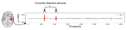
(a) EEG data

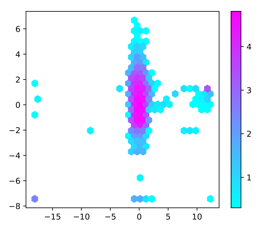
(b) Heatmap of http data

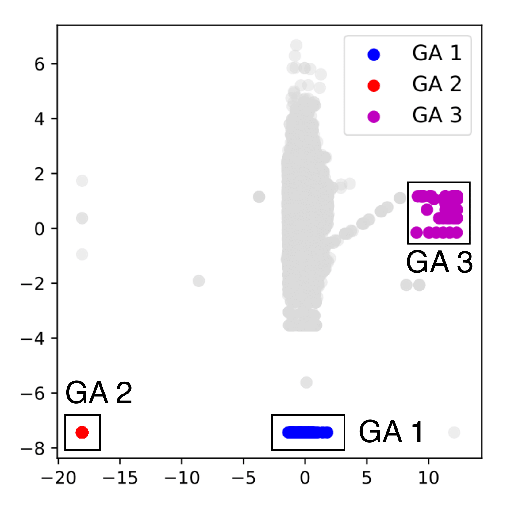
(c) Detected group-anomalies

 

Figure 1: (a) gen²Out matches ground truth. Brain scan of the patient with electrode positions (left), and detected groups shown in color red (right), that matches the ground truth seizure locations. (b) Heatmap of http intrusion detection dataset (c) gen²Out correctly spots group (DDoS) attacks in the intrusion detection dataset, marked GA1, GA2 and GA3.

As suggested by the application domain, to achieve better outcomes for patients, it is critical to direct attention of the clinician to the anomalous time periods in the brain activity in order of their suspiciousness. The problem is two-fold: (a) detection, as well as (b) ranking of generalized anomalies. We want a scoring function for generalized anomalies, such that in the EEG/epilepsy setting it would score the groups which may correspond to anomalous periods e.g. seizure and draw attention to most anomalous time periods; thus aiding a domain expert in decision making. As we show in Section III-A, we propose some intuitive axioms, that a generalized anomaly detector should obey.

Informal Problem 1 (Doubly-general anomaly problem).

• Given a point-cloud dataset from an application setting,

• find the point-anomalies and group-anomalies, and

• rank them in suspiciousness order.

Generality of approach: In most machine learning (ML) algorithms, we operate on clouds of points (after embedding, after auto-encoding etc). For example, time series is transformed into some form of $m-$dimensional cloud [3] for further analysis; in images, numerical features are generated for learning tasks e.g. Imagenet [16]. Thus, the proposed approach can be applied to diverse real data including point cloud, time-series and image data.

Figure 1 illustrates the effectiveness of our method – gen²Out detects group-anomalies that correspond to seizure period in the patient; and, detects DoS/DDoS attack as group-anomalies.

We propose gen²Out, which has the following properties:

• Principled and Sound: We identify five axioms (see Section §III-A) and show that the proposed gen²Out obeys them, in contrast to top competitors.

• Doubly-general: gen²Out is doubly general. First dimension of generalization is size of anomalies – detecting point- and group-anomalies. Second dimension of generalization is scoring and ranking of generalized anomalies– both point- and group-anomalies.

• Scalable: Linear on the input size (see Figure 10).

• Effective: Applied on real-world data (see Figure 1 and 7), gen²Out wins in most cases over benchmark datasets for point anomaly detection. For group anomaly detection, gen²Out has no competitors as they need group structure information, and it agrees with ground truth on seizure detection.

Reproducibility: Our source code and public datasets are at https://github.com/mengchillee/gen2Out. Our epilepsy EEG dataset involves real patients and requires NDA.

TABLE I: gen²Out matches all the specs. Qualitative comparison of gen²Out against top competitors showing that every competitor misses one or more features.

	LODA [20]	RRCF [10]	IF [17]	OCSMM[19]	AAE-VAE[7]	MGM[29]	GLAD [30]	gen2Out
Obeys Axioms (see §III-A)				?	?	?	?	✓
Discover point anomalies	✓	✓	✓					✓
Rank point anomalies	✓	✓	✓					✓
Discover group anomalies							?	✓
Rank group anomalies				✓	✓	✓	✓	✓
Jointly rank point- and group- anomalies								✓
Scalable	✓	?	✓	?	✓	?	?	✓

II Background and Related Work

Anomaly detection is a well-studied problem. Recent works [4, 8, 1, 11, 25] provide a detailed review of many methods for anomaly and outlier detection. As shown in Table I, gen²Out is the only method that matches the specs. Here, we review anomaly detection methods for point- and -group- anomalies.

Point Anomaly Detection. Model-based and density-based methods for outlier detection are quite popular for point cloud data. Principal component analysis (PCA) based detectors [24] assume that the data follows a multi-variate normal distribution. Local outlier factor (LOF) [5] flags instances that lie in low-density regions. Clustering based methods [12] score instances or small clusters by their distance to large clusters. However, these methods suffer from too many false positives as they are not optimized for detection [18]. Recently, a surge of focus has been on ensemble-based detectors that have been shown to outperform base detectors and are considered state-of-the-art for outlier detection [9]. Isolation forest [17] (iF), a state-of-the-art ensemble technique, builds a set of randomized trees that allows approximating the density of instances in a random feature subspace. Emmott et al.  [9](2015) show that iF significantly outperforms other detectors such as LOF. iF [17] shows that LOF has a high computation complexity (quadratic) and does not scale for large datasets. After that two more methods LODA [20] and Random Cut Forests (RRCF) [10] have been proposed as state-of-the-art methods. LODA is projection-based histogram ensemble that works well in many real settings. RRCF improve upon iF and use a data sketch that preserves pairwise distances.

Group Anomaly Detection. Numerous methods have been proposed for group anomaly detection [19, 7, 29, 30]. Earlier approaches [19, 7, 29] require the group memberships of the points known apriori, while Yu et al. [30] requires information on pairwise relations among data points. Moreover, these methods focus only on scoring group-anomalies, and ignore point-anomalies unlike our method. gen²Out detects and ranks anomalous points and groups, without requiring additional information on group structure of the dataset. As mentioned above, Table I summarizes comparison of gen²Out against state-of-the-art point- and group- anomaly detection methods. As such none of the methods has all the features of Table I .

Fractals and multifractals: In order to stress test our method, we use self-similar (fractals) clouds of points. We created the fractal images (Sierpinski triangle, biased line and ‘fern’ etc.), using the method and the code from Barnsley and Sloan [2]. We used the ‘uniform’ version (that is, for the Sierpinski triangle, all the miniature versions have the same weight of 1/3), also generated the ‘biased’ version of triangle using weights (0.6, 0.3, 0.1), and ‘biased line’ with bias $b=0.8$ using weights (0.8, 0.2) that is $b$ of the data points go to the first half of the line, and in this half, $b$ of the data points go to first quarter of the line, and so on recursively (this, informally, is the 80-20 law).

III Proposed Axioms and Insights

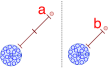
(a) A1: Distance Axiom

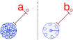
(b) A2: Density Axiom

(c) A3: Radius Axiom

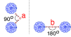
(d) A4: Angle Axiom

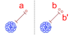
(e) A5: Group Axiom

Figure 2: Illustration of Axioms

In this section, we explain our proposed axioms in detail and give the insights. It is worth noting that these axioms are proposed to examine whether an anomaly detector is provided with the ability to compare the scores across datasets. The assumption is that, there are two different datasets with the same application setting. Although some of the axioms seem to be popular in single dataset setting, they are not considered and even ever mentioned by other studies when there is more than one dataset. The observed insights are critical and penetrate this research. These greatly inspire us on selecting the core part of our anomaly detector.

III-A Proposed Axioms

We propose five axioms an ideal anomaly detector should follow: producing higher anomaly scores when an instance is farther away from data kernel (distance aware), or lies in low density locality (density, radius and group aware), and not aligned with majority of data (angle aware [14]). In the following, let $\boldsymbol{a}\in\mathrm{R}^{m}$ and $\boldsymbol{b}\in\mathrm{R}^{m}$ be $m-$dimensional anomalies in point cloud datasets $S_{a}$ and $S_{b}$ respectively. Additionally, suppose that normal observations are distributed uniformly in a disc in the datasets as shown in Figure 2 and $s(.)$ is the generalized anomaly score function.

Axiom A1 (Distance Aware).

All else being equal, the farther point from the normal observations is more anomalous.

$$\left.\begin{array}[]{l}S_{a}-\{\boldsymbol{a}\}=S_{b}-\{\boldsymbol{b}\},\\ dist(\boldsymbol{a},S_{a})>dist(\boldsymbol{b},S_{b})\\ \end{array}\right\}\implies s(\boldsymbol{a})>s(\boldsymbol{b})$$

Axiom A2 (Density Aware).

All else being equal, denser the cluster of points, more anomalous the outlier.

$$\left.\begin{array}[]{l}dist(\boldsymbol{a},S_{a})=dist(\boldsymbol{b},S_{b}),\\ density(S_{a})>density(S_{b})\\ \end{array}\right\}\implies s(\boldsymbol{a})>s(\boldsymbol{b})$$

Axiom A3 (Radius Aware).

All else being equal, for a given number of observations, smaller the radius of the cluster of points, more anomalous the outlier.

$$\left.\begin{array}[]{l}|S_{a}|=|S_{b}|,\\ dist(\boldsymbol{a},S_{a})=dist(\boldsymbol{b},S_{b}),\\ radius(S_{a})<radius(S_{b})\end{array}\right\}\implies s(\boldsymbol{a})>s(\boldsymbol{b})$$

Axiom A4 (Angle Aware).

All else being equal, smaller the angle of a point with respect to cluster of observation, more anomalous the outlier.

$$\left.\begin{array}[]{l}|S_{a}|=|S_{b}|,\\ density(S_{a})=density(S_{b}),\\ radius(S_{a})=radius(S_{b}),\\ angle(\boldsymbol{a},S_{a})<angle(\boldsymbol{b},S_{b})\\ \end{array}\right\}\implies s(\boldsymbol{a})>s(\boldsymbol{b})$$

Axiom A5 (Group-size Aware).

All else being equal, the least populous group, the more anomalous it is.

$$\text{Let }g_{a}\subset S_{a},g_{b}\subset S_{b}\text{ are the {group}{s}}.$$

$$\left.\begin{array}[]{l}|g_{a}|<|g_{b}|\\ |S_{a}-g_{a}|=|S_{b}-g_{b}|,\\ density(S_{a})=density(S_{b}),\\ radius(S_{a})=radius(S_{b}),\\ \end{array}\right\}\implies s(g_{a})>s(g_{b})$$

Justification for Axioms Axiom A1 is self explanatory as shown in Figure 2a. The outlier point (shown in color red) in the left dataset (Figure 2a) being farther from the normal observations should be more anomalous.

Consider the case of social networks. A node reachable via $k$ hops from a close friends group should be more anomalous compared to reachable via $k$ hops from a colleagues group. Figure 2b illustrates Axiom A2 where the outlier in the left dataset should be more anomalous.

As shown in Figure 2c, for the same number of observations, the larger radius cluster would have a larger distance among points. Therefore, the outlier in the left dataset with smaller radius should be more anomalous.

The farther points would tend to form a smaller angle with the cluster of observations (see Figure 2d) and should be more anomalous in the left dataset.

The group $g_{a}=\{\boldsymbol{a}\}$ consisting of one point Figure 2e is intuitively more anomalous compared to group $g_{b}=\{\boldsymbol{b},\boldsymbol{b}^{\prime}\}$ containing more data points. For example, if $g_{b}$ has $1000$ points, it is not an anomaly anymore.

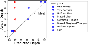
Figure 3: gen²Out wins (in color blue) as the estimated depth is close to $45^{o}$ line. iF estimates the same depth for each dataset with $\#$samples=1M.

III-B Insights

In this section, we are given the observations $X=\{\boldsymbol{x_{1}},\dots,\boldsymbol{x_{n}}\}$ where $\boldsymbol{x_{i}}\in\mathrm{R}^{m}$ (see Table II for symbol definitions) for the anomaly detection. Our goal is to design an anomaly detector that obeys the axioms proposed in §III-A. The intuition for the selection of basic model is that, according to the five axioms in Figure 2, point ‘a’ in the first dataset should always have higher probability to be separated out comparing the point ‘b’ in the second dataset. atomicTree has the properties which are very close to our demand. Here, we consider a randomized tree atomicTree data structure with the following properties – (i) Each node in the tree is either leaf node, or an internal node with two children, (ii) internal nodes store an attribute-value pair and dictate tree traversal. Given $X=\{\boldsymbol{x_{1}},\dots,\boldsymbol{x_{n}}\}$, atomicTree is grown through recursive division of $X$ by randomly selecting an attribute and a split value until all the leaf nodes contain exactly one instance (hence the name atomicTree) of observations assuming that observations are distinct. We randomly generate more than one tree to build a forest, to reduce the variance and detect outliers in subspaces.

We make a number of interesting observations while empirically investigating the process of tree growth for a variety of data distributions including multi-fractals. In Figure 4h, we report depth (height) distribution of randomized trees averaged over $100$ trees. We sample a number of points ($|X|\in\{2^{10},2^{11},2^{12},2^{20}\};m=2$) from each data distribution (shown in Figure 4h (a), (b), (c), (d), (i), (j), (k), (l)) and plot their corresponding depth (height) distribution (shown in Figure 4h (e), (f), (g), (h), (m), (n), (o), (p)). Notice that the number of points ($2^{\text{x}};\text{x}\in\{6,7,\dots\}$) in the tree grows linearly with the average depth for any given dataset. In Figure 3, we plot the predicted depth for each of the distributions against the actual depth of the tree for those distributions shown in Figure 4h by fitting to this linear trend. We present the following lemma based on the observations and draw the following insights.

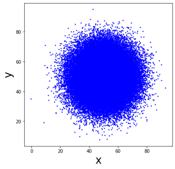
(a) One Normal

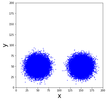
(b) Two Normals

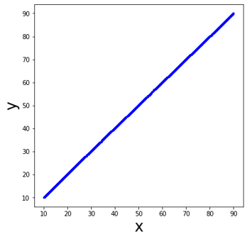
(c) Uniform Line

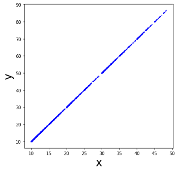
(d) Biased Line

(e) One Normal

(f) Two Normals

(g) Uniform Line

(h) Biased Line

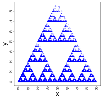
(k) Biased Sierpinski Triangle

(l) Uniform Square

(m) Fern

(o) Biased Sierpinski Triangle

(p) Uniform Square

(q) Fern

Figure 4: Illustrating depth distribution for several diverse datasets (including Gaussian, Uniform, multifractals).

Depth distributions



Depth distributions

(i)

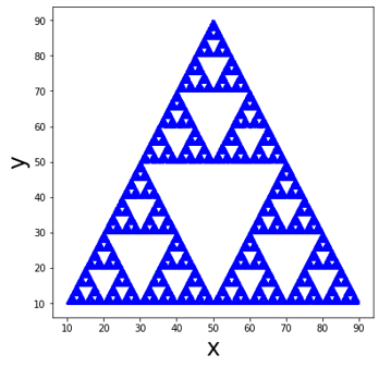
(j) Sierpinski Triangle

(n) Sierpinski Triangle

Insight 1 (Power Depth Property (PDP)).

The growth of the tree depth with the logarithm counts of observations is linear irrespective of the data distribution.

Justification for PDP property: In our attempt to explain PDP property, we study the expected depth computation for datasets with known distributions. However, in general, it is difficult. Let us consider biased line dataset with a bias factor $b$. Here we study a related setting: random points, but with fixed cuts. We refer to this model as ’fixed-cut’ tree fixedCutTree. For this case, we can show that the PDP property holds, and the slope grows as the ‘bias’ factor $b$ grows. Then, the depth of fixedCutTree for a biased fractal line (data in Fig. 4d) obeys the following lemma.

TABLE II: Table of symbols.

Symbol	Definition
$X=\{\boldsymbol{x_{i}}\}$	point cloud dataset where $\boldsymbol{x_{i}}\in\mathrm{R}^{m}$ for $i\in 1,2,\dots n$
$s(.)$	anomaly score function for an outlier detector
$h(\boldsymbol{q})$	path length estimate for instance $\boldsymbol{q}$ as it traverses
	a depth limited atomicTree
$\mathbb{E}[h(\boldsymbol{q})]$	path length averaged over the ensemble
$H(n)$	depth estimation function for an atomicTree
	containing $n$ observations
$d_{limit}$	depth limit of a atomicTree

Lemma 1 (Expected Depth of fixedCutTree).

The expected tree depth $H(n,b)$ for a biased line with a bias factor $b$ containing $n\geq 2$ data points is given as:

$$H(n,b) =\sum_{k=0}^{n}\big{[}{n\choose k}b^{k}(1-b)^{n-k}\times$$

$$\big{(}\frac{k}{n}H(k,b)+\frac{n-k}{n}H(n-k,b)+1\big{)}\big{]}$$

Proof. Let $H(k,b)$ be the depth of fixedCutTree with $k$ observations constructed using $X_{k}\subseteq X$. Since fixedCutTree is grown via recursive partitioning on a randomly chosen attribute-value, therefore, for a biased line, $b=$ probability of a point going to left node i.e. the point less than chosen attribute-value. Let $k$ be the number of points partitioned onto the left node, then $n-k$ points go to right node. Define $\mathrm{B}(n,k,b)={n\choose k}b^{n}(1-b)^{n-k}$ the Binomial probability for a fixed $k$. Let $f(n,k,b)$ be the estimate of the depth when $k$ observations are in left node, then $f(n,k,b)=\big{(}\frac{k}{n}H(k,b)+\frac{n-k}{n}H(n-k,b)+1\big{)}$ as each random partition increases depth by $1$. Therefore, the expected depth of the tree is given as $H(n,b)$ = $\sum_{k=0}^{n}f(n,k,b)\mathrm{B}(n,k,b)$. $\blacksquare$

We denote $H(n,b)=H(n)$ for $b=1/2$. A tree with one data point would have a depth of one i.e. $H(1,b)=1=H(1)$; and $H(0,b)=0=H(0)$. In Figure 5, we show the effect of bias on the the (analytical) depth computed using $H(n,b)$. Notice that increase in bias – indicating deviation from uniformity – increases depth which matches intuition.

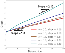
Figure 5: Depth ($\boldsymbol{H(n,b)}$) vs. Dataset size: slope increases with increase in bias for a biased line data

Corollary 1.

For bias $1-b$, $H(n,1-b)$ follow the results for $H(n,b)$.

Following the PDP property, the depth estimation function is given as

$$H(n)\approx w_{0}+w_{1}log_{2}(n)$$ (1)

where $w_{0}$ and $w_{1}$ are parameters that we estimate for each data distribution, and $n$ is the number of instances in the dataset.

Insight 2.

The slope of the linear fit varies significantly depending on the dataset distribution.

For example, the slope for Uniform Line (see Fig. 4g) is $1.38$, while for a Uniform Square (see Fig. 4p) is $1.66$. These insights lead to the following lemma.

Lemma 2.

gen²Out includes iF as a special case.

Proof. In Eq. 1, setting $w_{0}=2\times 0.57-(2(n-1)/n)$ and $w1=2\times log_{e}(2)$ yields the average path length function used in iF. Here, $0.57$ is the Euler’s constant, and $log_{e}(2)$ accounts for the difference in log bases. $\blacksquare$

Drawing from these insights, next we present the details of our proposed anomaly detector algorithm.

TABLE III: gen²Out wins as it obeys all the axioms a generalized anomaly detector should follow. We compare the methods statistically, by conducting two-sample t-test based on scores obtained for points $\boldsymbol{a},\boldsymbol{b}$. A positive difference in score indicates that the detector follows that axiom (see Figure 2). indicates that the detector follows the axiom, indicates that the detector does not obey the axiom.

	LODA		RRCF		iF		gen2Out
	Statistic	$p$-value	Statistic	$p$-value	Statistic	$p$-value	Statistic	$p$-value
A1: Distance Axiom	0	1	3.6	0.002**	2.1	0.054	11.4	1.2e-9***
A2: Density Axiom	7e15	2e-275***	-0.14	0.89	-10	8.6e-9***	25.2	1.7e-15***
A3: Radius Axiom	0	1	6.4	4.8e-6***	11.9	5.9e-10***	21.3	3.4e-14***
A4: Angle Axiom	6.6	3.2e-6***	17.5	9.6e-13***	-0.2	0.83	53.7	2.5e-21***
A5: Group Axiom	-14.7	1.8e-11***	1.1	0.27	0.95	0.35	28.2	2.6e-16***

IV Proposed Method

For ease of exposition, we describe the algorithm in two steps – gen²Out₀ for point anomalies, and then gen²Out for generalized anomalies.

Data: A data matrix $X$, number of atomicTree estimators numTrees, atomicTree depth limit $d_{limit}$

Result: $w_{0},w_{1}$ of depth estimation function $H(\cdot)$ and atomicTree ensemble

1 Initialize $Y$ and $Z$;

/* Estimating the function $H(\cdot)$ */

2

for $i=n_{1},n_{1}+1,\dots$;

  // a small $n_{1}$ e.g. 10

3 do

4       Draw $X_{s}\subset X\text{ s.t. }|X_{s}|=2^{i}$ ;

5       $F_{s}\leftarrow$ Construct-atomicTree ($X_{s}$, $\infty$);

6       $Z\leftarrow Z\cup~{}$ average depth of $F_{s}$ containing observations $X_{s}$;

7       $Y\leftarrow Y\cup~{}i$;

8      

9 end for

10$H(.)\leftarrow$ Fit linear regression $Y$ and $Z$;

11 $w_{0},w_{1}\leftarrow\texttt{coefficients}(H(.))$;

/* Construct the ensemble of atomicTree */

12 for t = 1 to numTrees do

13       ensemble $\leftarrow$ ensemble $\cup$ Construct-atomicTree ($X$, $d_{limit}$);

14      

15 end for

return $w_{0},w_{1},$ ensemble

Algorithm 1 gen²Out₀-Fit

IV-A Point anomalies – gen²Out₀

Given the observations $X=\{\boldsymbol{x_{1}},\dots,\boldsymbol{x_{M}}\}$ where $\boldsymbol{x_{i}}\in\mathrm{R}^{m}$, gen²Out₀’s goal is to detect and assign anomaly score to outlier points. gen²Out₀ uses an ensemble of depth-limited randomized tree atomicTree (§III-B) that recursively partition instances in $X$.

Definition 1 (Depth Limited atomicTree).

An atomicTree that is constructed by recursively partitioning the given set of observations $X$ until a depth limit $d_{limit}$ is reached or the leaf nodes contain exactly one instance.

As evidenced in prior works, the random trees induce shorter path lengths (number of steps from root node to leaf node while traversing the tree) for anomalous observations since the instances that deviate from other observations are likely to be partitioned early. Therefore, a shorter average path length from the ensemble would likely indicate an anomalous observation. Anomaly detection is essentially a ranking task where the rank of an instance indicates its relative degree of anomalousness. We next design anomaly score function for our algorithm to facilitate ranking of observations.

Data: A data matrix $X$,$d_{limit}$, currDepth:0

Result: atomicTree

1 Initialize atomicTree ;

2 if $d_{limit}$ $\leq$ currDepth or $|X|\leq 1$ then

3       return a leaf node of size $|X|$

4 else

5      pick an attribute at random from $X$;

6       pick an attribute value at random;

7       $X_{l}\leftarrow$ set of points on the left ($<$) of the chosen attribute-value pair;

8       $X_{r}\leftarrow$ set of points on the right ($\geq$) of the chosen attribute-value pair;

9       left $\leftarrow$ Construct-atomicTree ($X_{l}$,$d_{limit}$, currDepth + 1);

10       right $\leftarrow$ Construct-atomicTree ($X_{r}$,$d_{limit}$, currDepth + 1)

11      return an internal node with {left, right, {chosen attribute-value pair}}

12 end if

Algorithm 2 Construct-atomicTree

Proposed Anomaly Score.  We construct anomaly score using the path length $h(\boldsymbol{q})$ for each instance $\boldsymbol{q}\in\mathrm{R}^{m}$ as it traverses a depth limited atomicTree. The path length for $\boldsymbol{q}$ is $h(\boldsymbol{q})=h_{0}+H(l_{busy})\text{ if }l_{busy}>1;\text{ otherwise }h(\boldsymbol{q})=h_{0}$ where $h_{0}$ is the number of edges $\boldsymbol{q}$ traverses from root node to leaf node that contains $l_{busy}$ points in a depth limited atomicTree. When $l_{busy}>1$, we estimate the expected depth from the leaf node using $H(l_{busy})$ (uses Eq. 1). We normalize $h(\boldsymbol{q})$ by the average tree height $H(n)$ (height of atomicTree containing $n$ observations) for the depth limited atomicTree ensemble to produce an anomaly score $s(\boldsymbol{q},n)$ for a given observation $\boldsymbol{q}$. Referring to the PDP insights we presented in Section §III-B, we estimate the data dependent $H(\cdot)$ using Eq. 1 since the tree depth grows linearly with the number of observations (in $log_{2}$) in the tree (see Figure 4h). The slope of the linearity is characterized by underlying data distribution; each distribution follows a linear growth. The score function is

$$s(\boldsymbol{q},n)=2^{-\frac{\mathrm{E}[h(\boldsymbol{q})]}{H(n)}}$$ (2)

where $\mathrm{E}[h(\boldsymbol{q})]$ is the average path length of observation $\boldsymbol{q}$ in the atomicTree ensemble, $n$ is number of data points used to construct each atomicTree, and $H(n)$ is the function for estimating depth of the tree given in Eq. 1.

gen²Out₀ Parameter Fitting.  gen²Out is a depth limited atomicTree ensemble. The algorithm for fitting gen²Out₀ parameters is provided in Algorithms 1 and 2.

Data: A data matrix $X$, atomicTree ensemble

Result: Anomaly scores scores for observations in $X$

1 Initialize depths;

2 Initialize scores;

3 Initialize $l_{busy}$;

4$n\leftarrow$ numSamplesInatomicTree;

5 for $\boldsymbol{x}\in X$ do

6       depths $\leftarrow$ depths $\cup$ compute path-lengths for $\boldsymbol{x}$ (see §IV-A);

7      

8      $l_{busy}$$\leftarrow$ $l_{busy}$$\cup$ compute number of samples in leaf where traversal of $\boldsymbol{x}$ terminated ;

9      

10 end for

11for depth $\in$ depths, $l\in$ $l_{busy}$ do

12       $h=$depth$+H(l)$;

13       $s=2^{\frac{-h}{H(n)}}$;

14       scores $\leftarrow$ scores $\cup~{}s$;

15      

16 end for

17return scores;

18

Algorithm 3 gen²Out₀-Scoring

gen²Out₀ Scoring.  To assign anomaly scores to the instances in a data matrix $X$, the expected path length $\mathrm{E}(h(\boldsymbol{q}))$ for each instance $\boldsymbol{q}\in X$. $\mathrm{E}(h(\boldsymbol{q}))$ is estimated by averaging the path length after tree traversal through each atomicTree in gen²Out ensemble. We outline the steps to assign anomaly score to a data point using gen²Out₀ in Algorithm 3.

Initialize $n\leftarrow|X|$;

/* Step 0: Fit a sequence of gen²Out₀ */

1 for $qr\in\{1,1/2,1/4,\cdots\}$ do

2       Draw $X_{s}\subset X$ s.t. $|X_{s}|=n\times qr$;

3       gen²Out₀-$ensembles$ $\leftarrow$ gen²Out₀-$ensembles$ $\cup$ gen²Out₀-Fit ($X_{s}$, ., .);

4      

5 end for

6

/* Step 1: create X-ray plot */

7

8for e $\in$ gen²Out₀-$ensembles$ do

       /* generate score for specific qualification rate */

9       scores $\leftarrow$ scores $\cup$ gen²Out₀-Scoring(X, e);

10      

11 end for

/* Step 2: Apex extraction */

/* max score and qualification rate for each point across qualified datasets */

12 max_scores, max_qr $\leftarrow\arg\max(\texttt{scores})$ ;

13

/* select points with max score above threshold */

14 candidate-points $\leftarrow X$[max_scores $\geq$ $threshold$];

/* Step 3: Outlier grouping */

15 for r $\in$ unique(max_qr) do

       candidate-points_r ;

        // candidate points at this qualification rate

       /* identify more than one group per qualification rate */

16       clusters $\leftarrow$ $cluster$ candidate-points_r;

17      

18 end for

/* Step 4: Compute iso-curves */

19 for $cl$ $\in$ clusters do

       /* points similar to outlier at (score=1, qr=1) is more anomalous */

20       iso_scores $\leftarrow$ $\frac{2-ManhattanDistance([\frac{\log_{2}{max\_qr(\boldsymbol{a})}}{10}+1,max\_score(\boldsymbol{a})],[1,1])}{2}$ $\forall\boldsymbol{a}\in cl$;

21      

22 end for

/* Step 5: Scoring */

23 assign $\texttt{scores}\leftarrow median(\texttt{iso\_scores}(cl))\;\;\forall cl\in\texttt{clusters}\$

Algorithm 4 gen²Out

IV-B Full algorithm – gen²Out

gen²Out₀ can spot point-anomalies. How can design an algorithm that can spot both point- as well as group-anomalies, simultaneously?

The main insight is to exploit the less-appreciated ability of sampling to drop outliers, with high probability. How can we use this property to spot group-anomalies, of size, say $n_{g}$ (in a population of $n$ data points)? The idea is that, with a sampling rate of $n_{g}/n$, a point $\boldsymbol{a}$ of the group will probably be stripped of its cohorts, and thus behave like a point-anomaly, exhibiting a high anomaly score. For dis-ambiguation versus the sampling of gen²Out₀, we will refer to this sampling process as ‘qualification’, and to the corresponding rate as $qr$= qualification rate.

In more detail, to determine whether point $\boldsymbol{a}$ belongs to a group-anomaly, we compute its (gen²Out₀) score $s(\boldsymbol{a},qr)$ for several qualification rates $qr$; when the score peaks (say, at rate $n_{g}/n$) then $n_{g}$ is roughly the size of the group-anomaly (= micro-cluster) that $\boldsymbol{a}$ belongs to. Some definitions:

Definition 2 (X-ray-line).

For a given data point $\boldsymbol{a}$, the X-ray line is the function (score($\boldsymbol{a}$, qr) vs qr).

Definition 3 (X-ray plot).

For a cloud of $n$ points, the X-ray plot is the 2-d plot of all the $n$ X-ray-lines (one for each data point)

See Figure 6b for an example.

Definition 4 (Apex).

Apex of point $\boldsymbol{a}$ is the point (score, qr) with the highest anomaly score.

See Figure 6c for an example.

Algorithm  4 describes the steps of the proposed gen²Out. In summary, we find the X-ray plot (Step 1) and then find the apex point for every data point $\boldsymbol{a}$ (Step 2); keep the ones with high apex and then cluster the corresponding data points (Step 3); and then assign scores to the each group (Step 4 and Step 5).

Figure 6 illustrates the steps in gen²Out on a synthetic dataset that has two anomalous groups along with several point anomalies.

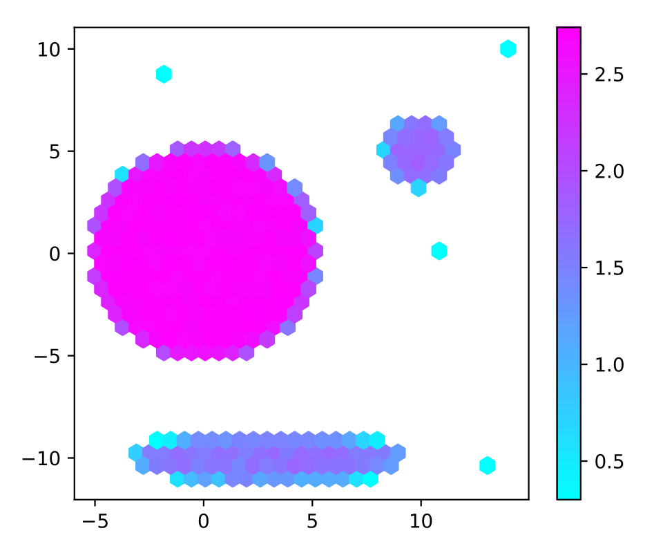
(a) Synthetic data heatmap

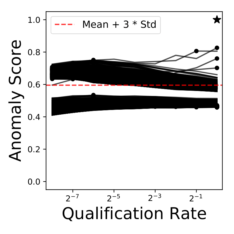
(b) Step 1: X-ray plot

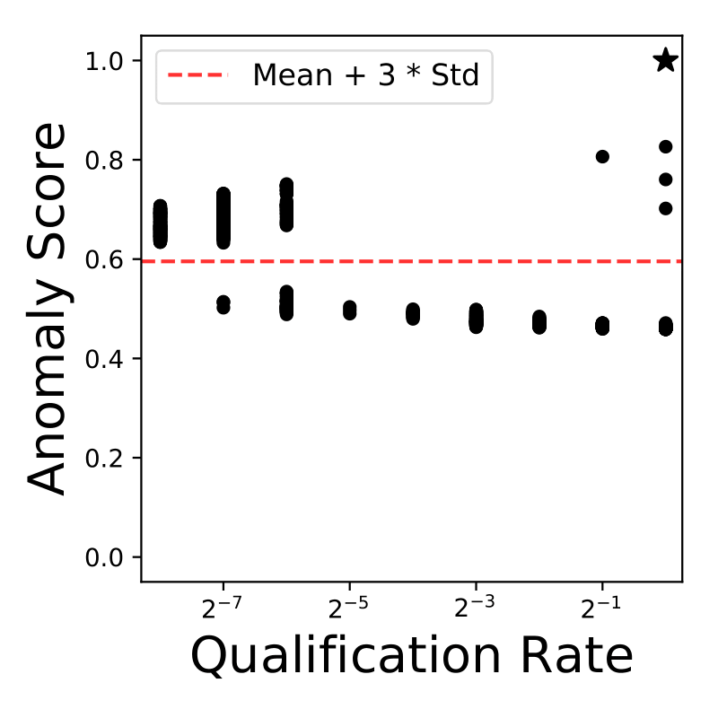
(c) Step 2: Apex extraction

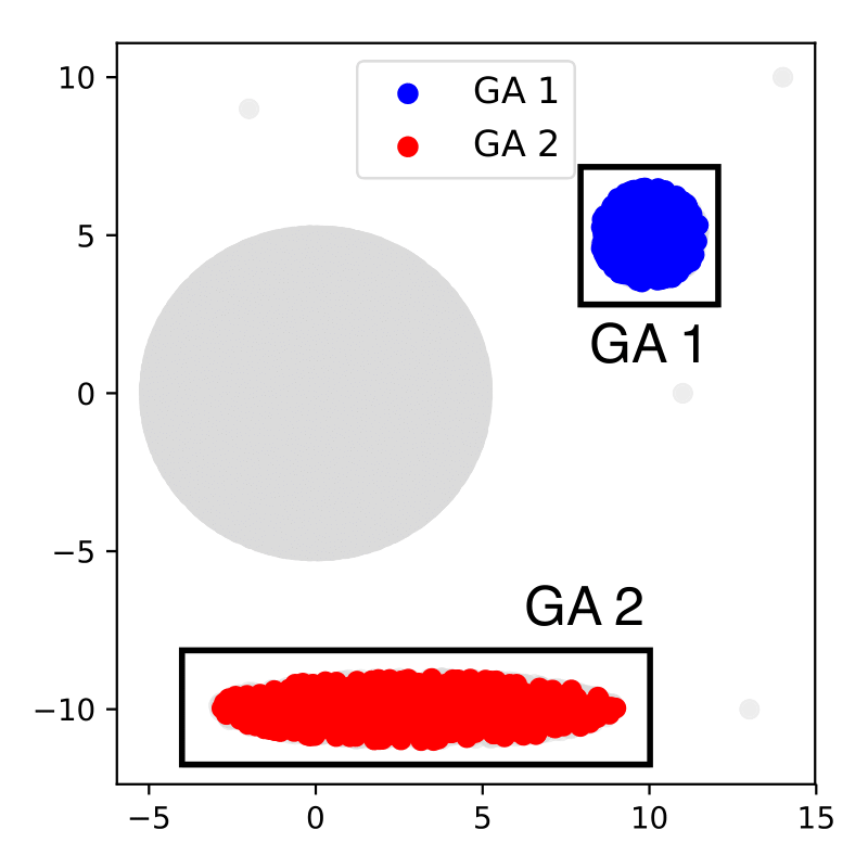
(d) Step 3: Outlier grouping

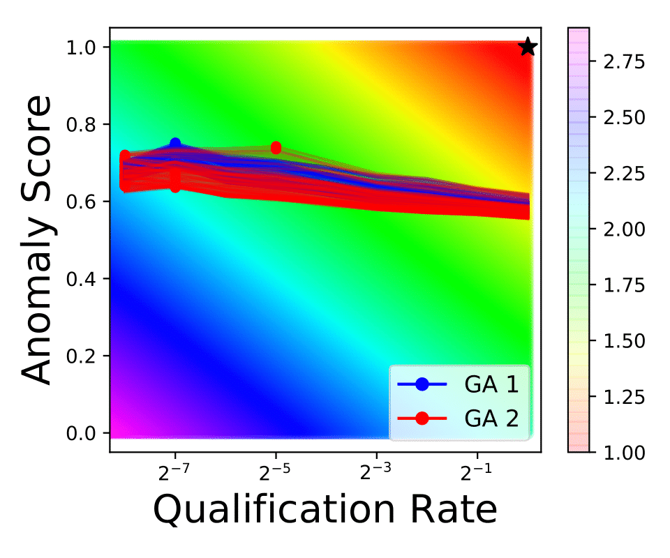
(e) Step 4: Anomaly iso-curves

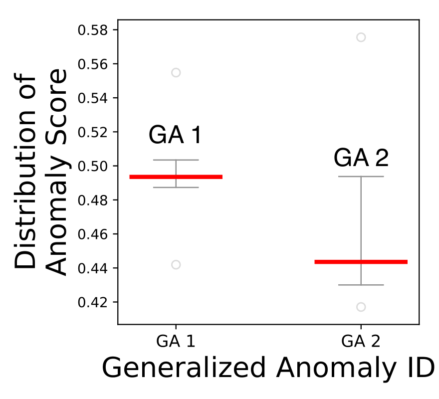
(f) Step 5: Scoring

Figure 6: gen²Out works. Illustration of gen²Out on synthetic dataset

Figure 6b finds the X-ray plot and Figure 6c shows the apex with the red threshold line. We find two groups after applying clustering (dbscan [22] in our implementation) shown in color red, and blue in Figure 6d. Then we compute the similarity of points in X-ray plot representation in each cluster to the theoretically most anomalous point at score$=1$, qr$=1$ (see iso curves in Figure 6e), and then assign generalized anomaly score using the median of the similarity scores as shown in Figure 6f. gen²Out correctly assigns higher score to GA1 (blue cluster in Figure 6f) which contains $1000$ points as compared to GA2 (red cluster in Figure 6f) containing $2000$ points (also see Axiom A5). For ease of visualization, we do not show point-anomalies in this plot.

V Experiments

TABLE IV: Benchmark datasets summary.

Datasets	#Samples	Dimension	% Outliers
$\text{Size}<3000$
arrhythmia	452	274	14.6%
cardio	1831	21	9.6%
glass	214	9	4.2%
ionosphere	351	33	35.9%
letter	1600	32	6.3%
lympho	148	18	4.1%
pima	768	8	34.9%
vertebral	240	6	12.5%
vowels	1456	12	3.4%
wbc	378	30	5.6%
breastw	683	9	35%
wine	129	13	7.8%
$\text{Size}\geq 3000$
mnist	7603	100	9.2%
musk	3062	166	3.2%
optdigits	5216	64	2.9%
pendigits	6870	16	2.3%
satellite	6435	36	31.6%
satimage-2	5803	36	1.2%
shuttle	49097	9	7.2%
annthyroid	7200	6	7.4%
cover	286048	10	0.96%
http	567498	3	0.39%
mammography	11183	6	2.3%
smtp	95156	3	0.032%
speech	3686	400	1.7%
thyroid	3772	6	2.5%

We evaluate our method through extensive experiments on a set of datasets from real world use-cases. We now provide dataset details and the experimental setup, followed by the experimental results.

V-A Dataset Description

• Epilepsy Dataset.  We analyzed intracranial electroencephalographic (EEG) signals recorded at the Epilepsy Monitoring Unit of a large public university from one patient with refractory epilepsy. Electrodes were stereotactically placed in the brain and EEG signals were then recorded across 122 electrode contacts at a sampling rate of 2KHz with focal region in the right temporal lobe.

• Benchmark Datasets.  Our benchmark set consist of 26 real-world outlier detection datasets from ODDS repository [21]. The datasets cover diverse application domains and have diverse range dimensionality and outlier percentage (summarized in Table IV). The ODDS datasets provide ground truth outliers that we use for the quantitative evaluation of the methods.

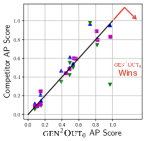
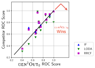
(a) Dataset size $<3000$.

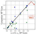
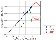
(b) Dataset size $\geq 3000$ where RRCF doesn’t scale.

Figure 7: gen²Out₀ wins. We plot average precision (AP) and area under the ROC curve for gen²Out₀ against the same metric of the competitors (none of which obey all our axioms). Points representing benchmark datasets are below the line for the majority of datasets.

(a) Data heatmap

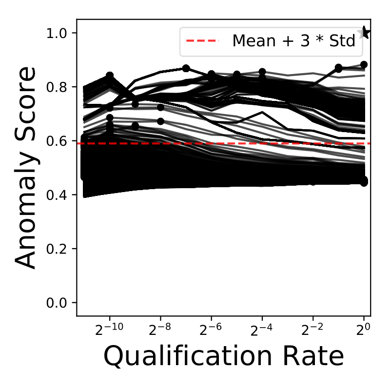
(b) X-ray plot

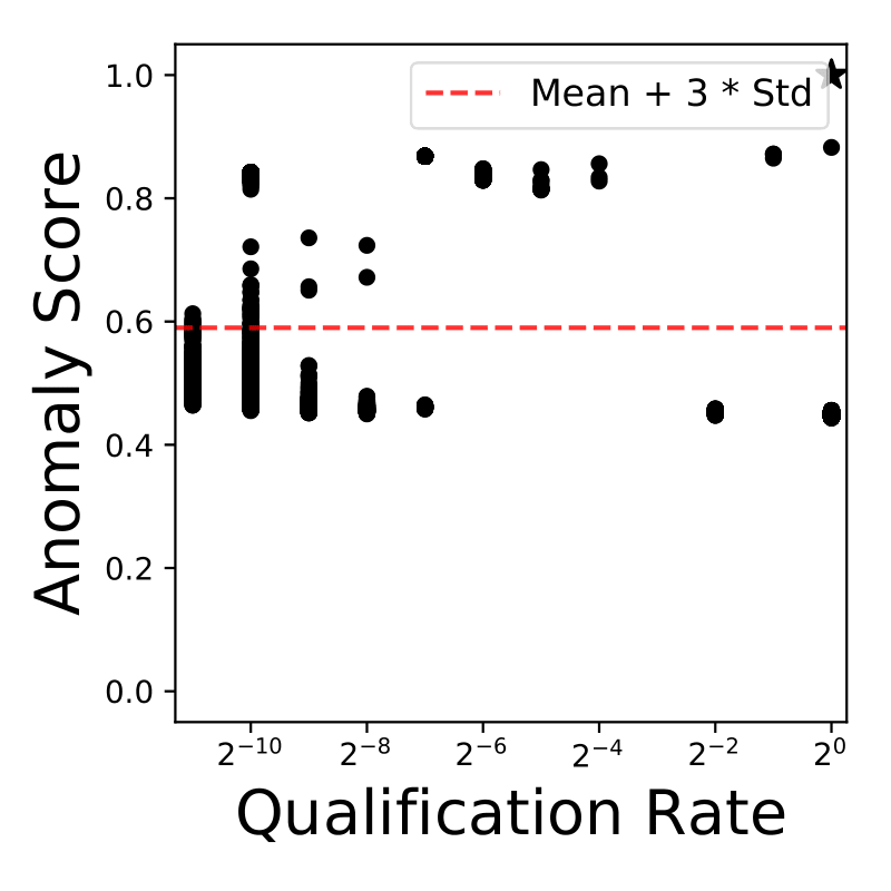
(c) Apex extraction

(d) Outlier grouping

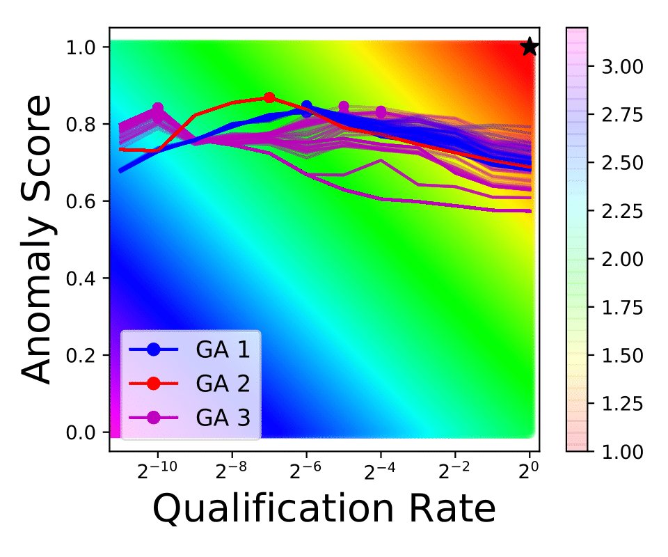
(e) Anomaly iso-curves

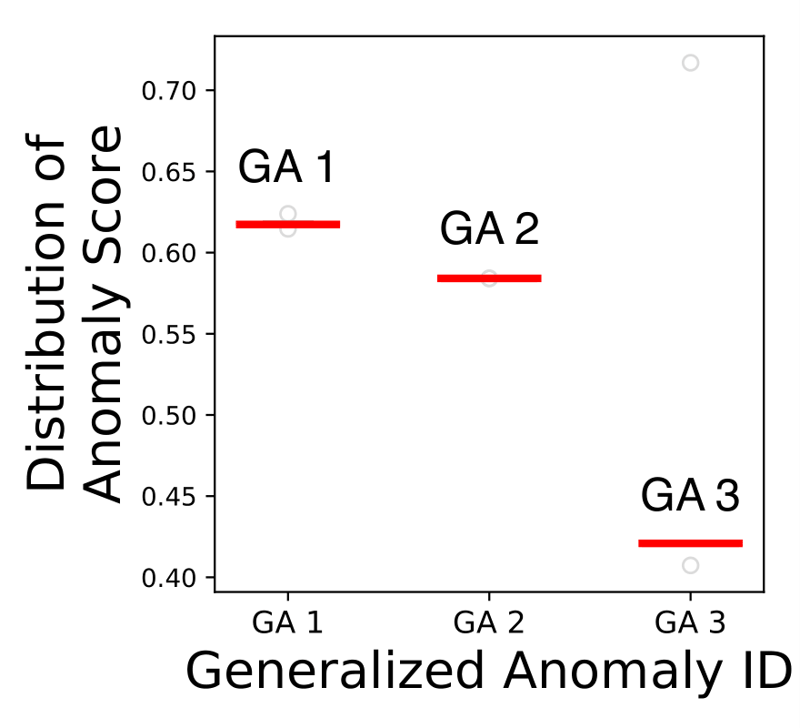
(f) Scoring

Figure 8: gen²Out detects DDoS attacks on intrusion detection http dataset

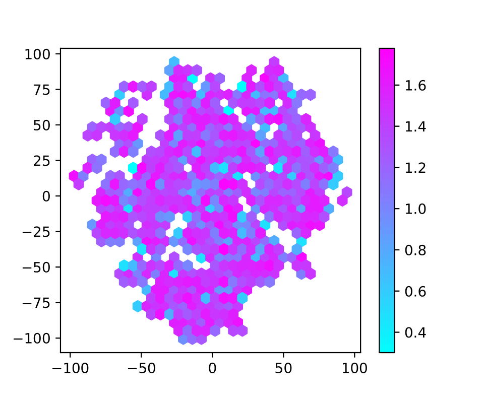
(a) Heatmap of tSNE representation of data

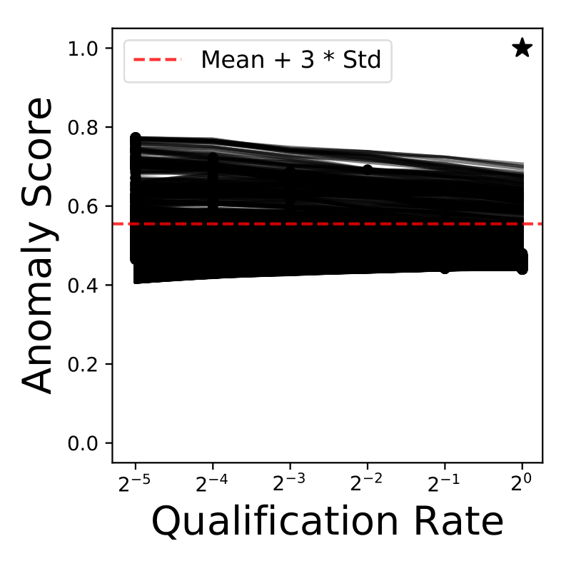
(b) X-ray plot

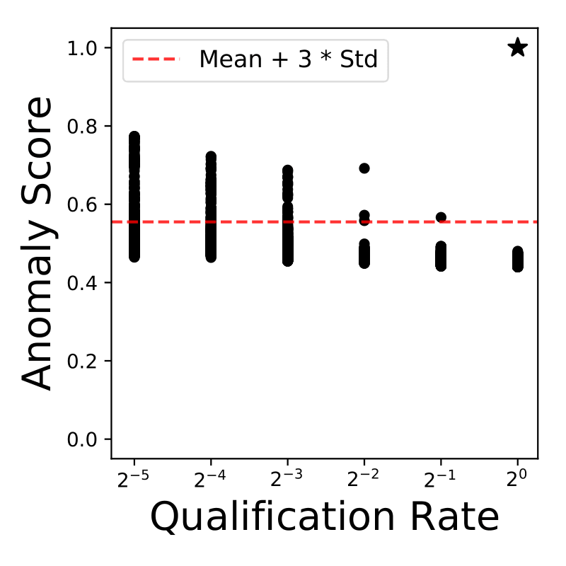
(c) Apex extraction

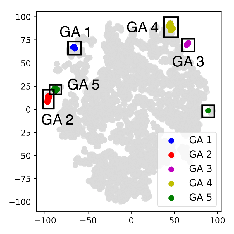
(d) Outlier grouping

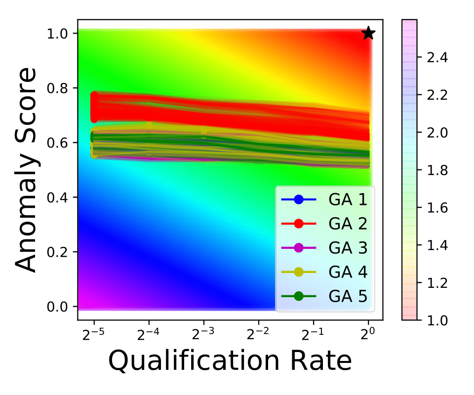
(e) Anomaly iso-curves

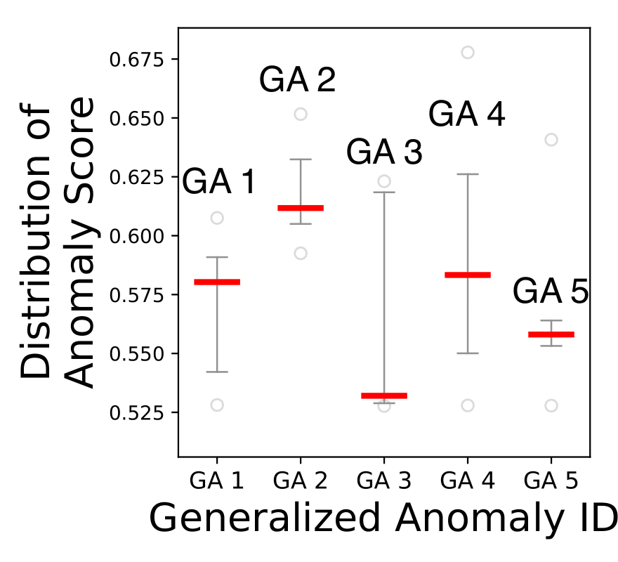
(f) Scoring

Figure 9: gen²Out works on real-world EEG data. Assigns highest anomaly score to group anomaly GA2 that corresponds to seizures as we show in Figure 1a.

V-B Point Anomalies

We compare gen²Out₀ to the following state-of-the-art ensemble baselines.

1. iF: Isolation Forest [17] uses an ensemble of randomized trees to flag anomalies.

2. LODA: Lightweight on-line detector of anomalies [20] is a projection based histogram ensemble.

3. RRCF: Robust Random Cut Forest [10] are tree ensembles that use sketch based anomaly detector.

To evaluate the effectiveness, we compare gen²Out₀ to state-of-the-art ensemble baselines on a set of real-world point-cloud benchmark outlier detection datasets. We use average precision (AP) and receiver operating characteristic (ROC) scores as our evaluation metrics. We plot the scores (AP and ROC score) for each competing method on all the benchmark datasets in Figure 7.

If the points are below the 45 degree line where each point represents a dataset listed in Table IV, then it indicates that gen²Out₀ outperforms the competition in those datasets. As shown in Figure 7, for both the evaluation metrics, gen²Out₀ beats or at least ties with all baselines on majority of the datasets (see Figure 1c). The quantitative evaluation demonstrates that gen²Out₀ is superior to its competitors in terms of evaluation performance as well as obeys all the proposed axioms while none of the competition obeys the axioms.

V-C Group Anomalies

We evaluate the effectiveness of gen²Out on real-world intrusion dataset that has attributes describing duration of attack, source and destination bytes. Note that we do not include group anomaly detection methods for comparison as they require group structure information, hence do not apply to our setting. Figure 8a shows source bytes plotted against destination bytes for the points. Figures 8b – 8f shows the X-ray plot with scores trajectory, Apex with candidate points above the threshold (set at mean + 3 standard deviation of scores in full dataset), identified groups and the generalized anomaly score for each detected group. gen²Out matches ground truth as it detects the three anomalous groups as shown in Figure 8d. In short gen²Out is able to detect groups that correspond to distributed-denial-of-service attack.

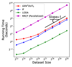
(a)

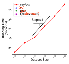
(b)

Figure 10: (a) gen²Out₀ is fast and scalable: Evaluation on benchmark datasets show that gen²Out (in red) scales linearly (eventual slope=1 in log-log scales). Note that none of the competitors obeys the axioms, and RRCF is significantly slower. (b) gen²Out is fast and scalable, linear in size of input.

V-D Scalability

To quantify the scalability, we empirically vary the number of observations in the chosen dataset and plot against the wall-clock running time (on 3.2 GHz 36 core CPU with 256 GB RAM) for the methods. First we compare gen²Out₀ against the competitors in Figure 10a for point-anomalies. The running time curve of gen²Out₀ is parallel to the running time curve of iF, which shows that gen²Out₀ does not increase time complexity except adding a small constant overhead for estimating the depth function $H(.)$. The running time of RRCF is much higher than others even after implementing the trees in parallel. Note that only gen²Out₀ obeys the axioms. For generalized anomalies, Figure 10b reports the wall-clock running time of gen²Out as we vary the data size. Notice that gen²Out scales linearly with input size. Importantly, competitors do not apply as they require additional information.

VI gen²Out at Work

VI-A No False Alarms.

When applied to datasets containing only normal groups that are relatively equal in size, gen²Out correctly identifies them as normal groups i.e. does not flag any set of points as anomalous group. To illustrate this phenomenon, we apply gen²Out to optdigits dataset which contains the feature representation of numerical digits.

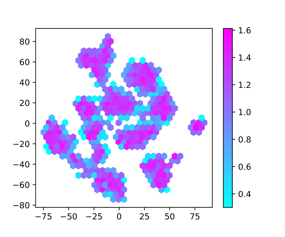
(a) Data heatmap

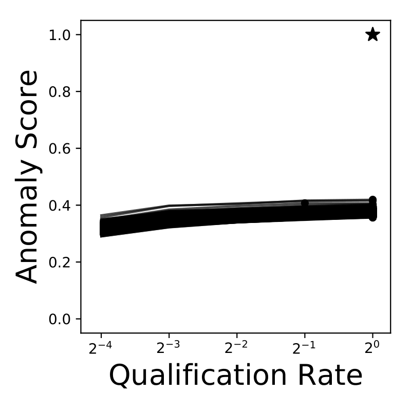
(b) X-Ray plot

Figure 11: gen²Out works. It correctly flags no anomalies in the optdigits dataset

To better visualize the dataset, we embed the points in two dimensional space using tSNE [27] as shown in Figure 11a. It is a balanced dataset, where we have equal number of points for each digit, hence no group is present. X-ray plot (Figure 11b) shows that all the score trajectories are below $0.5$ (scores close to $1$ are anomalous) with mean score at $0.36$ in full dataset. Hence, we do not find group and correctly so.

VI-B Attention Routing in Medicine.

We apply gen²Out on EEG recordings for the epileptic patient (PT1) – PT1 suffered through onset of two seizures in our recording clips; our motivating application. We extract four simple statistical measures from the subsequences of the time series features, namely mean, variance, skewness and kurtosis, by sliding a thirty minute window with two minutes overlap. Figure 9a shows $2-$dimensional tSNE representation of the data.

We then compute the generalized anomaly scores over time (within each window) for each detected group. Since the scores generated by gen²Out are comparable, we draw attention to the most anomalous time point, where the seizures occurred as the detected groups correspond to seizure time period. The steps of gen²Out are illustrated in Figure 9 when applied to multi-variate EEG data. Note that we find, several groups as shown in Figure 9. Of the detected groups, the group receiving highest score (GA2) is plotted over the raw voltage recordings over time for the patient. The group corresponds to the ground truth seizure duration (see Figure 1a). These time points that we direct attention to would assist the domain expert (in this case a clinician) in decision making by alleviating cognitive load of examining all time points.

VII Conclusions

We presented gen²Out – a principled anomaly detection algorithm that has the following properties.

• Principled and Sound: We propose five axioms that gen²Out obeys them, in contrast to top competitors.

• Doubly-general: Propose doubly general – simultaneously detects point and group anomalies – gen²Out. It does not require information on group structure, and ranks detected groups of varying sizes in order of their anomalousness.

• Scalable: Linear on the input size; requires minutes on 1M dataset on a stock machine.

• Effective: Applied on real-world data (see Figure 1 and 7), gen²Out wins in most cases over $27$ benchmark datasets for point anomaly detection, and agrees with ground truth on seizure detection as well as group detection tasks.

Reproducibility: Source code for algorithms are publicly available at https://github.com/mengchillee/gen2Out.

References

- [1] C. C. Aggarwal. Outlier analysis. In Data mining, pages 237–263. Springer, 2015.
- [2] M. F. Barnsley and A. D. Sloan. A better way to compress images. BYTE, 13(1):215–223, Jan. 1988.
- [3] A. Blázquez-García, A. Conde, U. Mori, and J. A. Lozano. A review on outlier/anomaly detection in time series data. ACM CSUR, 54:1–33, 2021.
- [4] A. Boukerche, L. Zheng, and O. Alfandi. Outlier detection: Methods, models, and classification. ACM Computing Surveys (CSUR), 53(3):1–37, 2020.
- [5] M. M. Breunig, H.-P. Kriegel, R. T. Ng, and J. Sander. Lof: identifying density-based local outliers. In ACM SIGMOD, pages 93–104, 2000.
- [6] N. Chakravarthy, S. Sabesan, K. Tsakalis, and L. Iasemidis. Controlling epileptic seizures in a neural mass model. Journal of Combinatorial Optimization, 17(1):98–116, 2009.
- [7] R. Chalapathy, E. Toth, and S. Chawla. Group anomaly detection using deep generative models. In ECML-PKDD, pages 173–189, 2018.
- [8] V. Chandola, A. Banerjee, and V. Kumar. Anomaly detection: A survey. ACM computing surveys (CSUR), 41(3):1–58, 2009.
- [9] A. F. Emmott, S. Das, T. Dietterich, A. Fern, and W.-K. Wong. Systematic construction of anomaly detection benchmarks from real data. In KDD - ODD workshop, pages 16–21, 2013.
- [10] S. Guha, N. Mishra, G. Roy, and O. Schrijvers. Robust random cut forest based anomaly detection on streams. In ICML, pages 2712–2721, 2016.
- [11] M. Gupta, J. Gao, C. C. Aggarwal, and J. Han. Outlier detection for temporal data: A survey. IEEE TKDE, 26(9):2250–2267, 2013.
- [12] Z. He, X. Xu, and S. Deng. Discovering cluster-based local outliers. Pattern Recognition Letters, 24(9-10):1641–1650, 2003.
- [13] T. Hutson, D. Pizarro, S. Pati, and L. D. Iasemidis. Predictability and resetting in a case of convulsive status epilepticus. Frontiers in neurology, 9:172, 2018.
- [14] H.-P. Kriegel, M. Schubert, and A. Zimek. Angle-based outlier detection in high-dimensional data. In KDD, pages 444–452, 2008.
- [15] B. Krishnan, I. Vlachos, Z. Wang, J. Mosher, I. Najm, R. Burgess, L. Iasemidis, and A. Alexopoulos. Epileptic focus localization based on resting state interictal meg recordings is feasible irrespective of the presence or absence of spikes. Clinical Neurophysiology, 126(4):667–674, 2015.
- [16] A. Krizhevsky, I. Sutskever, and G. E. Hinton. Imagenet classification with deep convolutional neural networks. Advances in neural information processing systems, 25:1097–1105, 2012.
- [17] F. T. Liu, K. M. Ting, and Z.-H. Zhou. Isolation forest. In ICDM, pages 413–422. IEEE, 2008.
- [18] F. T. Liu, K. M. Ting, and Z.-H. Zhou. Isolation-based anomaly detection. ACM Transactions on Knowledge Discovery from Data (TKDD), 6(1):1–39, 2012.
- [19] K. Muandet and B. Schölkopf. One-class support measure machines for group anomaly detection. arXiv preprint arXiv:1303.0309, 2013.
- [20] T. Pevnỳ. Loda: Lightweight on-line detector of anomalies. Machine Learning, 102(2):275–304, 2016.
- [21] S. Rayana. Odds library, 2016.
- [22] E. Schubert, J. Sander, M. Ester, H. P. Kriegel, and X. Xu. Dbscan revisited, revisited: why and how you should (still) use dbscan. ACM TODS, 42:1–21, 2017.
- [23] S. Shorvon. Epilepsy. Oxford Neurology Library. OUP Oxford, 2009.
- [24] M.-L. Shyu. A novel anomaly detection scheme based on principal component classifier. In Proc. ICDM Foundation and New Direction of Data Mining workshop, 2003, pages 172–179, 2003.
- [25] E. Toth and S. Chawla. Group deviation detection methods: a survey. ACM CSUR, 51:1–38, 2018.
- [26] K. Tsakalis and L. Iasemidis. Control aspects of a theoretical model for epileptic seizures. International Journal of Bifurcation and Chaos, 16(07):2013–2027, 2006.
- [27] L. Van der Maaten and G. Hinton. Visualizing data using t-sne. JMLR, 9, 2008.
- [28] I. Vlachos, B. Krishnan, D. M. Treiman, K. Tsakalis, D. Kugiumtzis, and L. D. Iasemidis. The concept of effective inflow: application to interictal localization of the epileptogenic focus from ieeg. IEEE Transactions on Biomedical Engineering, 64(9):2241–2252, 2016.
- [29] L. Xiong, B. Póczos, J. Schneider, A. Connolly, and J. VanderPlas. Hierarchical probabilistic models for group anomaly detection. In AISTATS, pages 789–797, 2011.
- [30] R. Yu, X. He, and Y. Liu. Glad: group anomaly detection in social media analysis. ACM Transactions on Knowledge Discovery from Data (TKDD), 10(2):1–22, 2015.