Laplace-like resonances with tidal effects

The first three Galilean satellites of Jupiter, Io, Europa, and Ganymede, move in a dynamical configuration known as the Laplace resonance, which is characterized by a 2:1 ratio of the rates of variation in the mean longitudes of Io-Europa and a 2:1 ratio of Europa-Ganymede. We refer to this configuration as a 2:1&2:1 resonance. We generalize the Laplace resonance among three satellites, $S_{1}$, $S_{2}$, and $S_{3}$, by considering different ratios of the mean-longitude variations. These resonances, which we call Laplace-like, are classified as first order in the cases of the 2:1&2:1, 3:2&3:2, and 2:1&3:2 resonances, second order in the case of the 3:1&3:1 resonance, and mixed order in the case of the 2:1&3:1 resonance. We consider a model that includes the gravitational interaction with the central body together with the effect due to its oblateness, the mutual gravitational influence of the satellites $S_{1}$, $S_{2}$, and $S_{3}$ and the secular gravitational effect of a fourth satellite $S_{4}$, which plays the role of Callisto in the Galilean system. In addition, we consider the dissipative effect due to the tidal torque between the inner satellite and the central body. We investigate these Laplace-like resonances by studying different aspects: $(i)$ we study the survival of the resonances when the dissipation is included, taking two different expressions for the dissipative effect in the case of a fast- or a slowly rotating central body, $(ii)$ we investigate the behavior of the Laplace-like resonances when some parameters are varied, specifically, the oblateness coefficient, the semimajor axes, and the eccentricities of the satellites, $(iii)$ we analyze the linear stability of first-order resonances for different values of the parameters, and $(iv)$ we also include the full gravitational interaction with $S_{4}$ to analyze its possible capture into resonance. The results show a marked difference between first-, second-, and mixed-order resonances, which might find applications when the evolutionary history of the satellites in the Solar System are studied, and also in possible actual configurations of extrasolar planetary systems.

1 Introduction

The Laplace resonance is a well-known configuration that was discovered by P.-S. de Laplace during his observations of the Galilean satellites of Jupiter: Io, Europa, Ganymede, and Callisto. The resonance consists of a set of commensurability relations between the mean longitudes $\lambda_{1}$, $\lambda_{2}$, and $\lambda_{3}$, and the longitudes of perijoves $\varpi_{1}$, $\varpi_{2}$, and $\varpi_{3}$,

$$\lambda_{1}-2\lambda_{2}+\varpi_{1} = 0$$

$$\lambda_{1}-2\lambda_{2}+\varpi_{2} = 180^{\circ}$$

$$\lambda_{2}-2\lambda_{3}+\varpi_{2} = 0\ .$$ (1)

We denote by $\Phi_{L}$ the Laplace angle defined as

$$\Phi_{L}\equiv\lambda_{1}-3\lambda_{2}+2\lambda_{3}\ ;$$ (2)

due to (1), $\Phi_{L}=180^{\circ}$, which implies that a triple conjunction between Io, Europa, and Ganymede can never be applied. Lieske (1998) observed (see also Paita et al. (2018)) that the Galilean satellites are such that $\Phi_{L}=180^{\circ}$ up to a libration with small amplitude and period of about 2071 days.

We consider a generalization of (1) by assuming that the resonance relation between the mean longitudes and the longitudes of pericenters involves combinations of the form $j\lambda_{1}-k\lambda_{2}$, $m\lambda_{2}-n\lambda_{3}$ that we denote as a j:k&m:n resonance. We adopt the following terminology:

• when both $j-k=1$ and $m-n=1$, we speak of a first-order Laplace-like resonance;

• if $j-k=2$ and $m-n=2$, we speak of a second-order Laplace-like resonance;

• when $j-k=2$ and $m-n=1$, or $j-k=1$ and $m-n=2$, we speak of a mixed-order Laplace-like resonance.

We consider the set of resonances including the 2:1&2:1, 3:2&3:2, 3:1&3:1, 2:1&3:1, and 2:1&3:2 resonances.

Although we worked with data and initial conditions corresponding to the Galilean satellites, many examples of first. and second-order resonances exist. They are typically found in satellite systems as well as in extrasolar planetary systems. To mention some examples, multiple mean-motion commensurabilities of three of the largest Uranian satellites were studied in Tittemore & Wisdom (1988): Miranda and Umbriel are in a 3:1 mean motion resonance, Miranda and Ariel are in a 5:3 resonance, and Ariel and Umbriel are in a 2:1 resonance. Another example of multi-body resonance is observed in the satellite system of Pluto because its satellites Styx, Nix, Kerberos, and Hydra are close to 3:1, 4:1, 5:1, and 6:1 resonances, respectively, with Charon, the largest moon of Pluto. Furthermore, according to Showalter & Hamilton (2015), the satellites Styx, Nix, and Hydra are in a 3:2&3:2 resonance. In addition to the Solar System, a few examples of three-body Laplace-like resonances have been observed in extrasolar planetary systems. According to Christiansen et al. (2018), the K2-138 extrasolar planetary system contains five sub-Neptune planets that are close to a first-order 3:2 resonant chain. Similar to this system, HD 158259 is the host star of five planets that are close to a 3:2 resonance chain (see Hara et al. (2020)). Another well-known example of resonance chains of planets is TRAPPIST-1 (Luger et al. (2017)), where the seven known planets are in a chain of Laplace resonances. An analytical model of multiplanetary resonant chains has been developed in Delisle (2017) and was applied to the four planets orbiting Kepler-223. Finally, the planetary system around the young star V1298 Tauri consists of four planets, two of which are in a 3:2 resonance (see David et al. (2019)). Other systems with chains of first-order resonances were presented in Pichierri et al. (2019).

The evolutionary history of the Galilean satellites has been studied by many authors. It is commonly accepted that dissipative tidal effects play a dominant role (Lainey et al. (2009), Malhotra (1991), Showman & Malhotra (1997), Tittemore (1990), Yoder (1979), Yoder & Peale (1981)). In particular, as mentioned in Tittemore (1990), while Io and Europa are assumed to be captured in a 2:1 resonance very soon after formation, Europa and Ganymede might have been in a 3:1 resonance in their early evolutionary history. We try to explore this scenario by exploring similarities and differences between the different sets of resonances mentioned before. We remark that we considered all mutual interactions between the satellites, while Tittemore (1990) considered only the interaction between Europa and Ganymede.

We performed a thorough analysis that led to a clear distinction between first-, second-, and mixed-order resonances. Our results are based upon a model that includes the gravitational effect of the central planet, the mutual gravitational interactions of the satellites, the effects due to the oblateness of the planet, and the secular gravitational interaction with $S_{4}$. We also considered the tidal interaction between $S_{1}$ and the central body, which is described by a set of equations affecting the evolution of the semimajor axis, eccentricity, and inclination (Ferraz-Mello et al. (2008)). In the remarkable paper de Sitter (1928), W. de Sitter investigated the question of whether the Laplace resonance is maintained under dissipation. This means that the three satellites should increase their semimajor axes in such a way that the ratios of the mean motions are kept fixed. It is then conjectured that the angular momentum acquired by Io from Jupiter is transferred to Europa, and then from Europa to Ganymede so that the Laplace resonant configuration survives. The conclusion drawn in de Sitter (1928) is that a condition for the survival of the Laplace resonance is that the effect of the dissipation is small; when it is large, the semimajor axes do not adjust, and the consequence is that the commensurability is destroyed in the course of time. We attach this question in the more general context of Laplace-like resonances because they are interesting in solar and extrasolar multibody systems other than the Galilean satellites.

We approached the problem by starting to investigate the sensitivity to the initial conditions and parameters involved, as well as by examining the changes in the dynamical evolution of a system of three satellites in different first-, second-, and mixed-order resonances. Next, we studied the linear stability of the first-order resonances, which are found to preserve the resonant dynamics as some parameters are varied.

Finally, we investigated the possibility that a fourth satellite that revolves around the planet is captured into resonance when it is studied within the context of the different Laplace-like resonances. In the case of the classical Laplace resonance (i.e., the actual resonance between the Galilean satellites), Callisto is captured into resonance, as has been remarked in Lari et al. (2020) and Celletti et al. (2021). We extend the study to the other Laplace-like resonances and study theoretically the possibility of the trapping into resonance. Our analysis leads us to conclude that $S_{4}$ is captured into resonance when first-order resonances are considered, while this is not the case for second- and mixed-order resonances.

This work is organized as follows. In Section 2 we present the averaged and resonant Hamiltonians and the corresponding equations of motion. In Section 3 we provide the equations for the tidal interactions between the central body and the first orbiting body. We study by numerical experiments the conservation of the Laplace argument considering the cases of a fast-rotating and a slowly rotating central body. The focus of the study is on the evolution in time of the resonant arguments, that is, the orbital elements of the satellites, close to resonant initial conditions, and on varying system parameters. In Section 4 we study the linear stability of the first-order Laplace-like resonances. Section 5 describes the study of the capture into resonance of the fourth satellite. Finally, we add some conclusions in Section 6.

2 Hamiltonian model

To study the dynamical evolution of the three inner satellites around the central body, the following contributions need to be considered: the gravitational interaction due to the central body, the mutual gravitational interactions of the satellites, the gravitational effects due to the oblateness of the planet, and the secular gravitational interaction with satellite $S_{4}$ and a distant star, such as the Sun.

In our model, we make a simplification by retaining only the resonant and secular parts, so that the Hamiltonian we consider consists of the following contributions: (a) the Keplerian part representing the interaction between the satellites and the central body, (b) the secular part of the mutual gravitational interaction of the three satellites, (c) the resonant part of the mutual gravitational interaction of the three satellites, (d) the secular gravitational effects of the oblateness of the planet, and (e) the secular gravitational interaction with $S_{4}$ and a distant star. We mainly concentrate on the study of resonant configurations among the three inner satellites, $S_{1}$, $S_{2}$ , and $S_{3}$; only in Section 5 does the model include the full (not only secular) gravitational interaction with $S_{4}$. When different resonances are studied, only the resonant part of the Hamiltonian changes, and the other contributions are the same for all resonances.

To compute the Hamiltonian function that describes our model, we adopted the following definitions: $m_{0}$ is the mass of the central planet, and $m_{j}$ is the mass of the $j$-th satellite. The orbital elements of the $j$-th satellite are the semi-major axis $a_{j}$, the eccentricity $e_{j}$, the inclination $I_{j}$ with respect to the equatorial reference frame, the mean longitude $\lambda_{j}$, the longitude of the pericenter $\varpi_{j}$, and the longitude of the ascending node $\Omega_{j}$. In addition, we introduce the auxiliary variable $s_{j}=\sin(I_{j}/2)$. We briefly describe the different contributions to the Hamiltonian below and refer to Celletti et al. (2019) for full details.

The Keplerian part can be written as

$$H_{Kep}=-{{\mathcal{G}M_{1}\mu_{1}}\over{2a_{1}}}-{{\mathcal{G}M_{2}\mu_{2}}\over{2a_{2}}}-{{\mathcal{G}M_{3}\mu_{3}}\over{2a_{3}}},$$

where $\mathcal{G}$ is the gravitational constant and the following auxiliary variables are introduced:

$$M_{1} = m_{0}+m_{1},\qquad M_{2} = M_{1}+m_{2},\qquad M_{3} = M_{2}+m_{3}$$

$$\mu_{1} = \frac{m_{0}m_{1}}{M_{1}},\qquad\mu_{2} = \frac{M_{1}m_{2}}{M_{2}},\qquad\mu_{3} = \frac{M_{2}m_{3}}{M_{3}}.$$

The secular and resonant Hamiltonians describing the mutual interaction of the satellites depend on the specific resonance that is studied. When we consider a specific resonance, we can write the Hamiltonian for the interaction between satellites $S_{U}$ and $S_{V}$ in the form

$${H_{P}}^{U,V}=-\mathcal{G}\frac{m_{U}m_{V}}{a_{V}}\Big{\{}F_{sec}(a_{U},a_{V},e_{U},e_{V},s_{U},s_{V})$$

$$+F_{res}(a_{U},a_{V},e_{U},e_{V},s_{U},s_{V},\lambda_{U},\lambda_{V},\varpi_{U},\varpi_{V},\Omega_{U},\Omega_{V})\Big{\}},$$

where $F_{sec}$ and $F_{res}$ denote the secular part and the resonant term, respectively, the latter being a trigonometric function that we truncate to second order in $e_{U},e_{V},s_{U},\text{and }s_{V}$. We provide in Appendix A the explicit expressions of the Hamiltonian ${H_{P}}^{U,V}$ for each resonant case.

The contribution due to the oblateness of the planet, limited to the secular terms, is given by

$$H_{obl}= -\sum_{i=1}^{3}\frac{\mathcal{G}M_{i}\mu_{i}}{2a_{i}}\bigg{[}J_{2}\left(\frac{R_{J}}{a_{i}}\right)^{2}\left(1+\frac{3}{2}e_{i}^{2}-\frac{3}{2}s_{i}^{2}\right)$$

$$-\frac{3}{4}J_{4}\left(\frac{R_{J}}{a_{i}}\right)^{4}\left(1+\frac{5}{2}e_{i}^{2}-\frac{5}{2}s_{i}^{2}\right)\bigg{]},$$

where $R_{J}$ is the radius of the planet, and $J_{2}$ is the spherical harmonic coefficient of degree two.

The part of the Hamiltonian that represents the secular gravitational attraction of the fourth satellite or a distant star is given by

$$H_{\sigma} =-\sum_{i=1}^{3}\Bigg{[}\frac{\mathcal{G}m_{i}m_{\sigma}}{a_{\sigma}}\left\{\frac{1}{2}b_{1/2}^{(0)}\left(\frac{a_{i}}{a_{\sigma}}\right)-1+\frac{1}{8}\frac{a_{i}}{a_{\sigma}}b_{3/2}^{(1)}\left(\frac{a_{i}}{a_{\sigma}}\right)(e_{i}^{2}+e_{\sigma}^{2})\right\}$$

$$-\frac{\mathcal{G}m_{i}m_{\sigma}}{a_{\sigma}}\left\{-\frac{1}{2}\frac{a_{i}}{a_{\sigma}}b_{3/2}^{(1)}\left(\frac{a_{i}}{a_{\sigma}}\right)(s_{i}^{2}+s_{\sigma}^{2})\right\}\Bigg{]},$$

where $\sigma=4$ refers to the secular interaction of the fourth satellite, $\sigma=Sun$ refers to the secular interaction by a distant star, such as the Sun in the case of the Laplace resonance, and ${b_{n}}^{(s)}$ are the Laplace coefficients (Murray & Dermott (1999)).

The final Hamiltonian is given by the sum of the following contributions:

$$H=H_{Kep}+{H_{P}}^{1,2}+{H_{P}}^{2,3}+{H_{P}}^{1,3}+H_{obl}+H_{4}+H_{Sun}.$$ (3)

It is convenient to express the Hamiltonian in modified Delaunay variables, which are given by

$$L_{i}=\mu_{i}\sqrt{\mathcal{G}M_{i}a_{i}}$$

$$P_{i}=L_{i}(1-\sqrt{1-{e_{i}}^{2}})\qquad for\quad i=1,2,3$$

$$\Sigma_{i}=L_{i}\sqrt{1-{e_{i}}^{2}}(1-\cos I_{i})$$

with conjugate angles $\lambda_{i}$, $p_{i}=-\varpi_{i}$ , and $\sigma_{i}=-\Omega_{i}$.

In the classical Laplace resonance between Io, Europa, and Ganymede, the longitudes and the arguments of perijove of the three satellites are found to satisfy relations (1), and the Laplace angle $\Phi_{L}$ defined in Eq. (2) is shown to librate around the value $\Phi_{L}=180^{o}$. In this case, we speak of a 2:1&2:1 resonance because Eq. (1) includes the combinations of the longitudes $\lambda_{1}-2\lambda_{2}$, $\lambda_{2}-2\lambda_{3}$. We generalize Eq. (1) by considering j:k&m:n resonances that involve combinations of the longitudes of the form $j\lambda_{1}-k\lambda_{2}$, $m\lambda_{2}-n\lambda_{3}$.

	3:2&3:2	2:1&3:2	2:1&2:1
$q_{1}$	$3\lambda_{2}-2\lambda_{1}-\varpi_{1}$	$2\lambda_{2}-\lambda_{1}-\varpi_{1}$	$2\lambda_{2}-\lambda_{1}-\varpi_{1}$
$q_{2}$	$3\lambda_{2}-2\lambda_{1}-\varpi_{2}$	$2\lambda_{2}-\lambda_{1}-\varpi_{2}$	$2\lambda_{2}-\lambda_{1}-\varpi_{2}$
$q_{3}$	$3\lambda_{3}-2\lambda_{2}-\varpi_{3}$	$3\lambda_{3}-2\lambda_{2}-\varpi_{3}$	$2\lambda_{2}-\lambda_{1}-\varpi_{3}$
$q_{4}$	$5\lambda_{2}-2\lambda_{1}-3\lambda_{3}$	$3\lambda_{3}-4\lambda_{2}+\lambda_{1}$	$3\lambda_{2}-\lambda_{1}-2\lambda_{3}$
$q_{5}$	$\lambda_{1}-\lambda_{3}$	$\lambda_{1}-\lambda_{3}$	$\lambda_{3}-3\lambda_{2}+2\lambda_{1}$
$q_{6}$	$\lambda_{3}$	$\lambda_{3}$	$\lambda_{2}+\frac{1}{3}(\lambda_{3}-\lambda_{1})$
$q_{7}$	$3\lambda_{2}-2\lambda_{1}-\Omega_{1}$	$2\lambda_{2}-\lambda_{1}-\Omega_{1}$	$2\lambda_{2}-\lambda_{1}-\Omega_{1}$
$q_{8}$	$3\lambda_{2}-2\lambda_{1}-\Omega_{2}$	$2\lambda_{2}-\lambda_{1}-\Omega_{2}$	$2\lambda_{2}-\lambda_{1}-\Omega_{2}$
$q_{9}$	$3\lambda_{3}-2\lambda_{2}-\Omega_{3}$	$3\lambda_{3}-2\lambda_{2}-\Omega_{3}$	$2\lambda_{3}-\lambda_{2}-\Omega_{3}$

	2:1&3:1	3:1&3:1
$q_{1}$	$2\lambda_{2}-\lambda_{1}-\varpi_{1}$	$3\lambda_{2}-\lambda_{1}-2\varpi_{1}$
$q_{2}$	$2\lambda_{2}-\lambda_{1}-\varpi_{2}$	$3\lambda_{2}-\lambda_{1}-\varpi_{1}-\varpi_{2}$
$q_{3}$	$3\lambda_{3}-\lambda_{2}-\varpi_{3}-\varpi_{2}$	$3\lambda_{3}-\lambda_{2}-\varpi_{3}-\varpi_{2}$
$q_{4}$	$3\lambda_{2}-3\lambda_{3}-\lambda_{1}+\varpi_{2}$	$4\lambda_{2}-3\lambda_{3}-\lambda_{1}-\varpi_{1}+\varpi_{2}$
$q_{5}$	$\lambda_{1}-\lambda_{3}$	$\lambda_{1}-\lambda_{3}$
$q_{6}$	$\lambda_{3}$	$\lambda_{3}$
$q_{7}$	$2\lambda_{2}-\lambda_{1}-\Omega_{1}$	$3\lambda_{2}-\lambda_{1}-2\Omega_{1}$
$q_{8}$	$2\lambda_{2}-\lambda_{1}-\Omega_{2}$	$3\lambda_{2}-\lambda_{1}-\Omega_{1}-\Omega_{2}$
$q_{9}$	$3\lambda_{3}-\lambda_{2}-\Omega_{3}-\Omega_{2}$	$3\lambda_{3}-\lambda_{2}-\Omega_{3}-\Omega_{2}$

Table 1: Angular coordinates for the different resonances

In the remaining paper we concentrate on the resonances 2:1&2:1, 3:2&3:2, 3:1&3:1, 2:1&3:2, and 2:1&3:1. We find it convenient to introduce new angular variables for each specific resonance that replace the angles $\lambda_{1}$, $\lambda_{2}$, $\lambda_{3}$, $\varpi_{1}$, $\varpi_{2}$, $\varpi_{3}$, $\Omega_{1}$, $\Omega_{2}$, and $\Omega_{3}$; to this end, we introduce the variables $q_{1},...,q_{9}$, as defined in Table 1. Especially in the case of the $2:1\&2:1$ resonance, the new set of angular variables was chosen by following Pucacco (2021). Table 2 presents the values of the masses, eccentricities, and inclinations of the Galilean satellites. These values are used throughout this paper in the numerical integrations of the equations of motion. In addition to the parameters, we used the initial conditions for the semimajor axes of the satellites that are shown in Table 3.

	$m_{j}$	$e_{j}$	$I_{j}$
Io	$8.933\times 10^{22}$	$4.721\times 10^{-3}$	$3.758\times 10^{-2}$
Europa	$4.797\times 10^{22}$	$9.819\times 10^{-3}$	$4.622\times 10^{-1}$
Ganymede	$1.482\times 10^{23}$	$1.458\times 10^{-3}$	$2.069\times 10^{-1}$
Callisto	$1.076\times 10^{23}$	$7.44\times 10^{-3}$	$1.996\times 10^{-1}$

Table 2: Values of the masses $m_{j}$, the eccentricities $e_{j}$ and the inclinations $I_{j}$ of the Galilean satellites.

	2:1&2:1	3:2&3:2	2:1&3:2
Io	$4.22\times 10^{5}$	$4.22\times 10^{5}$	$4.22\times 10^{5}$
Europa	$6.713\times 10^{5}$	$5.53\times 10^{5}$	$6.713\times 10^{5}$
Ganymede	$10.705\times 10^{5}$	$7.25\times 10^{5}$	$8.78\times 10^{5}$
Callisto	$18.828\times 10^{5}$	$12.751\times 10^{5}$	$15.442\times 10^{5}$

	3:1&3:1	2:1&3:1
Io	$4.22\times 10^{5}$	$4.22\times 10^{5}$
Europa	$8.78\times 10^{5}$	$6.713\times 10^{5}$
Ganymede	$18.26\times 10^{5}$	$13.94\times 10^{5}$
Callisto	$32.115\times 10^{5}$	$24.517\times 10^{5}$

Table 3: Initial values of the semimajor axes of the four satellites, expressed in kilometers.

3 Effect of tides on the dynamics

In this section we investigate the role of tides on the dynamics, that is, on the persistence of the Laplace-like resonances in the dissipative framework, and their effect on the orbital parameters in dependence of the system parameters (e.g., the dependence on the $J_{2}$ value and the initial orbital configuration in terms of semimajor axis $a$ and orbital eccentricity $e$).

3.1 Tidal models

The tidal interaction between the central body and the closest satellite affects the evolution of the semimajor axis, eccentricity, and inclination (Ferraz-Mello et al. (2008)). The equations describing the rates of variation in $a,e,\text{and }I$ due to the dissipation part that we used are

$$\begin{aligned} \frac{\dot{a}}{a}&=\frac{2}{3}c\left(1+\frac{51}{4}e^{2}-D(7e^{2}+{S_{B}}^{2})\right)\\ \frac{\dot{e}}{e}&=-\frac{1}{3}c\left(7D-\frac{19}{4}\right)\\ \dot{I}&=-\frac{3}{4}S_{B}c(1+2D)\ .\end{aligned}\quad.$$ (4)

The parameters $c$ and $D$ are defined as

$$c =\frac{9}{2}\frac{k_{0}}{Q_{0}}\frac{m_{1}}{m_{0}}\left(\frac{R_{0}}{a_{1}}\right)^{5}n_{1}$$ (5)

$$D =\frac{Q_{0}}{Q_{1}}\frac{k_{1}}{k_{0}}\left(\frac{R_{1}}{R_{0}}\right)^{5}\left(\frac{m_{0}}{m_{1}}\right)^{2},$$

where for j = 0,1 $k_{j}$ is the Love number, $Q_{j}$ is the quality factor, $k_{j}/Q_{j}$ is the tidal ratio, and $R_{j}$ is the radius of the central body and the innermost satellite, respectively. Moreover, $n_{1}$ is the mean motion of the first satellite, and $S_{B}=\sin(I_{1})$.

Equations (4), translated into Delaunay variables, was added to the equations for the variables $L,P,\text{and }\Sigma$ that can be derived from the Hamiltonian (3). Equations (4) hold when the central body rotates fast and under the assumption that the phase lags remain constant and are all equal. This tidal model is valid in the case of planetary satellites. However, when an extrasolar planetary system is studied, the central body rotates slowly. In this case, equations (4) can be modified as follows (Ferraz-Mello et al. (2008)):

$$\frac{\dot{a}}{a} =-\frac{2}{3}c\left(1+\frac{57}{4}e^{2}+7De^{2}\right)$$ (6)

$$\frac{\dot{e}}{e} =-\frac{1}{3}c\left(7D+\frac{25}{4}\right)$$

$$\dot{I} =-\frac{3}{4}S_{B}c(1+2D).$$

In the next sections, we investigate the dynamics of first- and second-order Laplace-like resonances with tidal torque for fast-rotating planets using Eq. (4) and slow rotating central bodies using Eq. (6). In our model the tidal effects are only considered between the central body and the innermost satellite. The interaction between the central body and the remaining moons can usually be neglected in this type of study.

3.2 Survival of the Laplace-like resonances under the tidal dissipation

In this section, we present the evolution of the Laplace angle that results from the numerical integrations in all five different first-, second-, and mixed-order resonances. The equations of motion were integrated numerically using a Runge-Kutta eighth-order scheme with a variable step size performed using a Wolfram Mathematica program. The resonant arguments that involve the longitudes of the three satellites are given in Table 4.

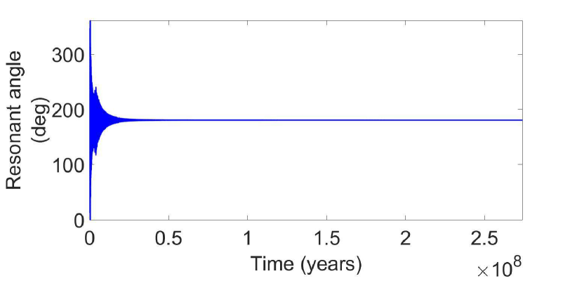
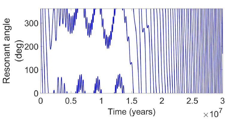
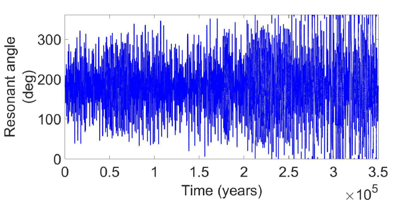
Figure 1: Evolution of the resonant argument in three cases: the 2:1&3:2 resonance considering a fast-rotating central body (top panel), the 2:1&3:1 resonance considering a fast-rotating central body (middle panel), and the 3:2&3:2 resonance considering a slowly rotating central body (bottom panel).

A major point in the study of the Laplace-like resonances is the survival of the resonance when the tidal effects between the central body and one or more satellites are considered. According to Ferraz-Mello (1979), the Laplace resonance is kept under a dissipative force, leading to quadratic inequalities in the mean longitudes. This question was already raised in de Sitter (1928). Lainey et al. (2009) used numerical integrations and stated that the Laplace resonance is destroyed because of the inward migration of Io and the outward migration of Europa and Ganymede. Recently, Lari et al. (2020) showed that the Laplace resonance is kept for about 1 Gyr, and then Callisto is captured into resonance with Ganymede. Lari et al. (2020) also studied the stability of the resonance after 1 Gyr using different initial conditions of Callisto and testing different scenarios. In most of the simulations, the Laplace resonance survives. In this section, we study the survival of the Laplace-like resonances taking the tidal interaction between the central planet and $S_{1}$ into account and considering the cases of a fast-rotating and slowly rotating central body, as described in Section 3.

3.2.1 Fast-rotating central body

In this section, we analyze the case of a fast-rotating central planet for which we consider the dissipation given by Eq. (4). For each resonance, we started by examining the behavior of the resonant argument, which corresponds to the angles listed in Table 4.

Resonance	Resonant argument
2:1&2:1	$2\lambda_{3}-3\lambda_{2}+\lambda_{1}$
3:2&3:2	$3\lambda_{3}-5\lambda_{2}+2\lambda_{1}$
2:1&3:2	$3\lambda_{3}-4\lambda_{2}+\lambda_{1}$
3:1&3:1	$3\lambda_{3}-4\lambda_{2}+\lambda_{1}$
2:1&3:1	$3\lambda_{3}-5\lambda_{2}+2\lambda_{1}$

Table 4: Resonant arguments in the different resonances that involve the mean longitudes of the three satellites.

During the evolution, we multiplied the tidal effect by a pumping factor $\alpha=10^{5}$ to increase the strength of the tides and speed up numerical integrations (in absence of the Hamiltonian contributions, the presence of $\alpha$ can be seen as a rescaling of time; see Showman & Malhotra (1997) and Lari et al. (2020)). Using as parameters the masses of the Galilean satellites and the initial conditions given in Tables 2 and 3, we find that the 2:1&2:1, 3:2&3:2, and 2:1&3:2 resonances survive under the dissipation, while the 3:1&3:1 and 2:1&3:1 resonances are destroyed by the dissipation in the sense that the resonant argument circulates instead of librating around a fixed value. This makes a marked difference between first-, second-, and mixed-order Laplace-like resonances evident. Figure 1 shows the sample of a first-order resonance with the Laplace argument trapped into libration (top panel) and a mixed-order resonance with an oscillation of the resonant angle (bottom panel).

3.2.2 Slowly rotating central-body

When the dissipation associated with a slowly rotating central body as in Eq. (6) is used, the situation is different from the fast-rotating planet case. In the classical 2:1&2:1 resonance, a migration of the closest satellite to the planet and a circulation of the resonant argument are observed. The same situation occurs for the 3:2&3:2 resonance, in which the decrease in semimajor axis of the inner satellite provokes a close encounter with the planet. Here as well as in the 2:1&3:2, 3:1&3:1, and 2:1&3:1 cases, the resonance is not preserved, and the resonant argument circulates after a short time interval. An example is given in Figure 1 (bottom panel), showing a short period of libration followed by a circulation of the Laplace angle.

As a conclusion, the choice of the tidal model strongly affects the presence of the resonant evolution of the Laplace angles because the variation rate of the semi-major axis has a different sign for fast and slow rotation. This is true for the actual Galilean system, but also for the other resonances.

3.3 Resilience of the Laplace-like resonances

In this section, we investigate the evolution of the orbital elements of the three satellites under the variation of the initial conditions and parameters that are involved in the model. As a first step, we study the evolution of the semimajor axes, eccentricities, and inclinations of the three satellites. We remark that they include the tidal effects between a fast-rotating central body and the inner satellite only. In some cases, the simultaneous migration of all three satellites is observed, as in the 3:2&3:2 and 2:1&3:2 resonances, while in the 3:1&3:1 resonance, only the inner satellite moves outward and the semimajor axes of the other two satellites remain constant. In the 2:1&3:1 resonance, the two inner satellites migrate and the semimajor axis of the third satellite remains constant. In addition, the eccentricity of the inner satellite converges to zero, while the eccentricity of the other two satellites oscillates around an average value. The results are presented in Figures 2 and 3 for the 3:2&3:2 and 3:1&3:1 resonances, respectively. Moreover, we analyze the behavior of the different resonances when varying $J_{2}$ (Section 3.3.1), the initial value of the semimajor axis (Section 3.3.2), and the initial value of the eccentricity (Section 3.3.3) in the case of the Laplace-like resonances

The increase in semimajor axis of the inner satellite is expected theoretically due to the tidal torque exerted by the fast-rotating central body. In the cases of first-order resonances, the migration of the inner satellite is transferred through the gravitational attractions to all the bodies, and as a result, they all migrate outward, maintaining the resonance. This can be seen, for example, in the case of the 3:2&3:2 resonance, where all three satellites move outward, while the three eccentricities converge to limit values. These results indicate a marked difference between first- and second-order resonances. The linear stability of first order is addressed in a semi-analytical way in Section 4.

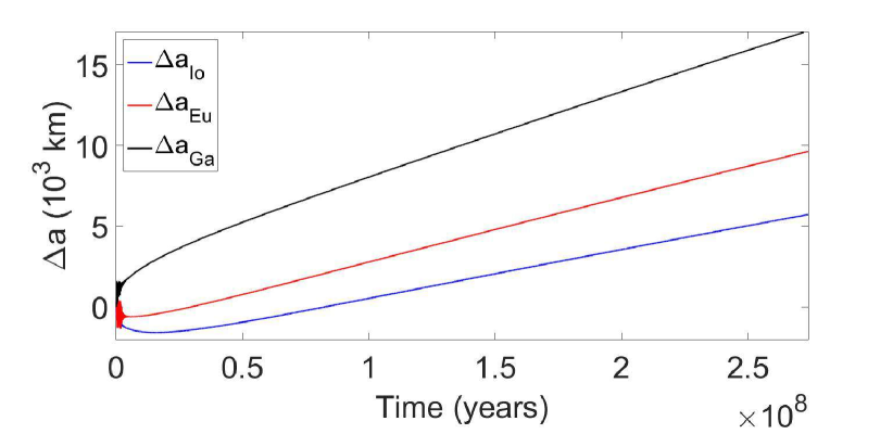
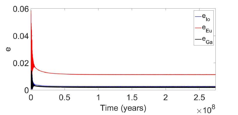
Figure 2: Variation in semimajor axes (top panel) and eccentricities (bottom panel) of the three satellites due to the dissipative effects between the planet and the inner satellite considering a fast-rotating central body and assuming a 3:2&3:2 resonance The tidal effects are multiplied by a factor of $\alpha=10^{5}$.

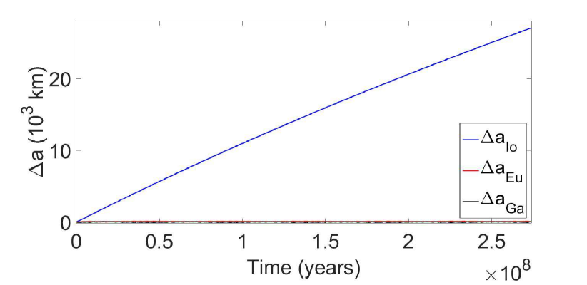
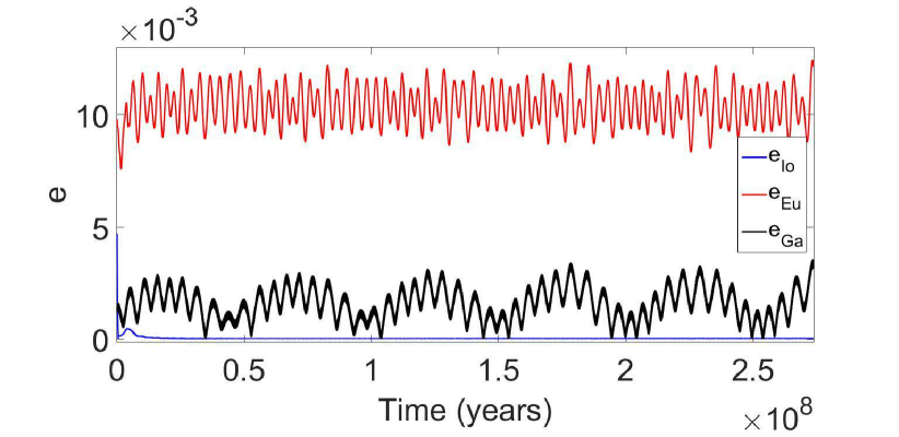
Figure 3: Variation in semimajor axes (top panel) and eccentricities (bottom panel) of the three satellites due to the dissipative effects between the planet and the inner satellite considering a fast-rotating central body and assuming a 3:1&3:1 resonance. The tidal effects are multiplied by a factor of $\alpha=10^{5}$.

The inclinations in the 2:1&3:2 and 2:1&3:1 resonances oscillate randomly, but remain close to the initial ones. In the 3:2&3:2 resonance, the inclinations converge to zero, while in the 3:1&3:1 resonance, they increase and are higher than the initial ones. We can conclude that in the 3:2&3:2 resonance, the planar model, which is simpler, would give reliable results. Instead, in the mixed- and second-order resonances and especially in the 2:1&3:1 resonance, the inclinations play an important role in the dynamics of the system (Figure 4).

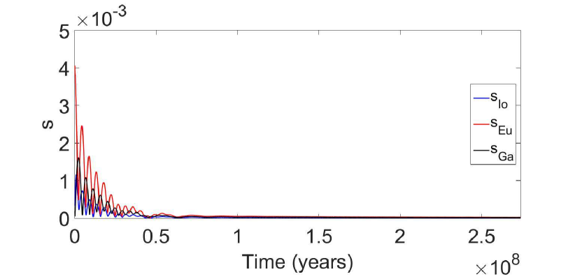
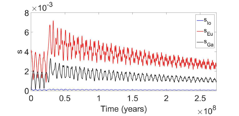
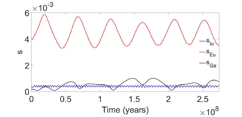
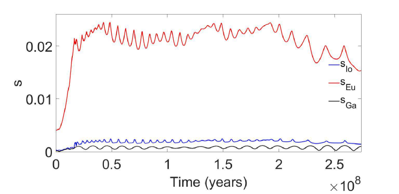
Figure 4: Variation in inclinations of the three satellites due to the dissipative effects between the planet and the inner satellite considering a fast-rotating central body. The four panels from top to bottom correspond to the 3:2&3:2, 2:1&3:2, 3:1&3:1, and 2:1&3:1 resonances. The tidal effects are multiplied by a factor of $\alpha=10^{5}$.

3.3.1 Dependence on the $J_{2}$ value of the central body

In the case of the 3:2&3:2 resonance, the effect due to the oblateness of the central body plays an important role in the evolution of the resonant argument. It is worth noting that the effects due to the oblateness of the central body induce an additional precession of the pericenters. When the $J_{2}$ value of the central planet is set equal to zero, the resonance is kept, but the resonant argument librates around $180^{\circ}$ with a higher amplitude than when the $J_{2}$ value is different from zero. In the case of the 2:1&3:2 resonance, the resonant argument librates around $180^{\circ}$, but when the oblateness of Jupiter is not taken into account, the resonant argument takes values from 0 to $360^{\circ}$ , and after some time, the resonant angle enters a librational regime.

In the case of the second-order resonances, the effect of the oblateness of the central planet can be observed in the evolution of the eccentricities of the three satellites. In the case of the 3:1&3:1 resonance, the eccentricity of the inner satellite converges to zero for all three values of $J_{2}$. When the $J_{2}$ value is equal to zero, an oscillation with a very small amplitude is observed in the case of the eccentricity of $S_{1}$, while the eccentricities of $S_{2}$ and $S_{3}$ oscillate with a larger amplitude. When the $J_{2}$ value is different from zero, the eccentricities of $S_{2}$ and $S_{3}$ oscillate around lower values with shorter frequencies (see Figure 5).

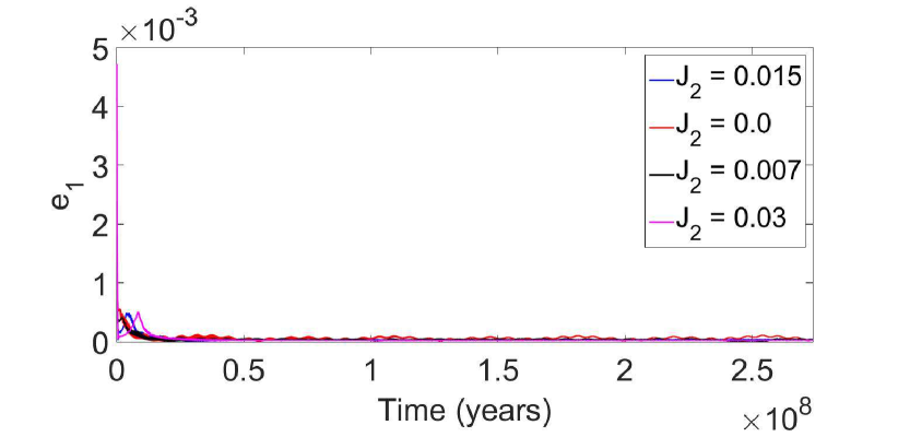
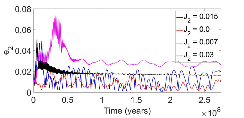
Figure 5: Evolution of the eccentricity of $S_{1}$ in the 3:1&3:1 resonance (top panel) and $S_{2}$ in the 2:1&3:1 (bottom panel) from the dissipative model using four different $J_{2}$ values of the central planet when the factor multiplying the tidal dissipation is $\alpha=10^{5}$.

In the case of the 2:1&3:1 resonance, the eccentricity of $S_{1}$ does not converge to zero when the $J_{2}$ value of the central body is different from the actual value. However, for all four values of $J_{2}$ we have taken as sample, the eccentricity oscillates around a value that is lower than the initial eccentricity. The eccentricities of $S_{2}$ and $S_{3}$ oscillate with a higher amplitude when the perturbation due to the oblateness of the central planet is not considered.

3.3.2 Dependence on the initial value of the semimajor axis

In this section, we investigate the sensitivity in the evolution of the orbital elements of the satellites on the initial value of the semimajor axis of the inner satellite by varying it using the relation $a_{0}(1\pm 10^{-3})$.

In the case of the 3:2&3:2 resonance, the semimajor axes of the three satellites increase, with the exception of the semimajor axis of the inner satellite, which decreases at the beginning and then increases. When the initial value of the semimajor axis of the inner satellite is lower, the initial decrease is larger and reaches lower values. On the other hand, the semimajor axes of $S_{2}$ and $S_{3}$ increase with a higher rate, using the lower initial value of the semimajor axis of the inner satellite (see Figure 6).

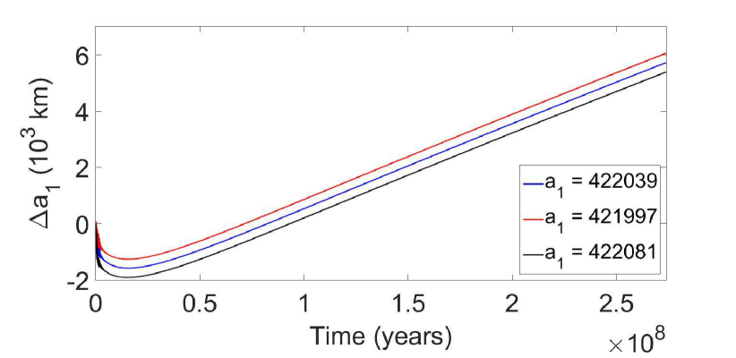
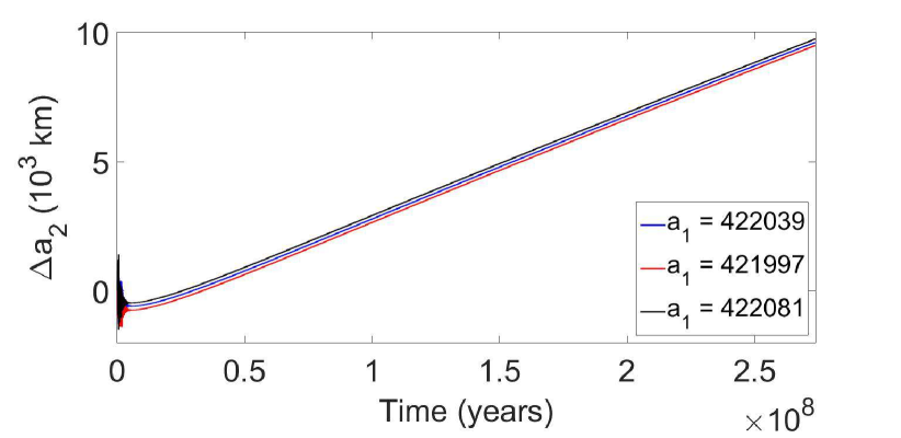
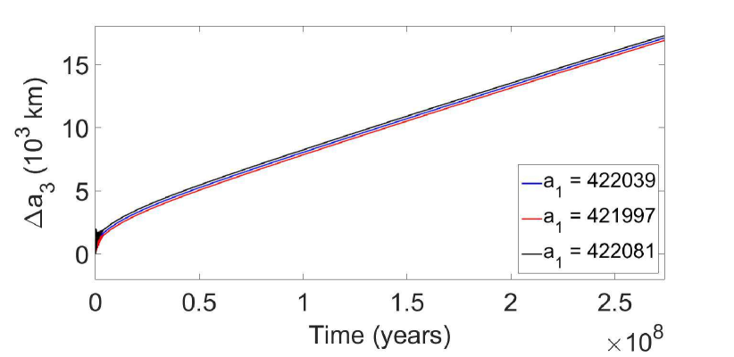
Figure 6: Variation in semimajor axes of $S_{1}$ (top panel), $S_{2}$ (middle panel), and $S_{3}$ (bottom panel) from the dissipative model assuming a 3:2&3:2 resonance and using three different initial values of semimajor axis of $S_{1}$ when the factor multiplying the tidal dissipation is $\alpha=10^{5}$. The tidal model assumes that the central body rotates fast. The different initial values of the semimajor axis of $S_{1}$ are $a_{10}=422039$ (the nominal one), $a_{10}=421997,$ and $a_{10}=422081$.

The semimajor axes of the three satellites in the case of the 2:1&3:2 resonance increase, and only the semimajor axis of the inner satellite shows a slight decrease at the beginning.

A different behavior is observed for second-order resonances. The semimajor axis of the inner satellite in the case of the 3:1&3:1 resonance increases, and the same effect is observed even when the initial value is changed. The semimajor axes of $S_{2}$ and $S_{3}$ remain constant and oscillate around a given value. The amplitude of the oscillations is larger when the initial value of the semimajor axis of the inner satellite is larger (see Figure 7).

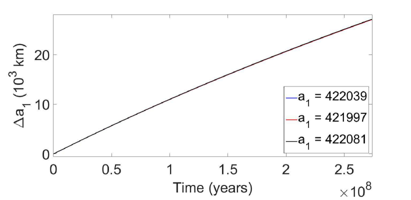
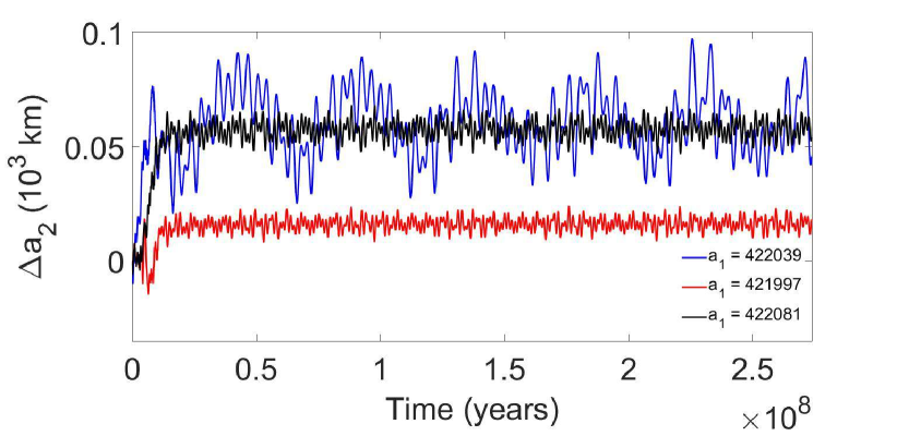
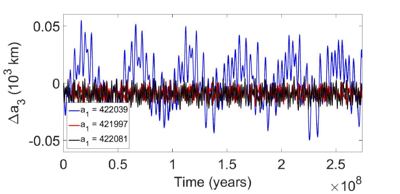
Figure 7: Variation in semi-major axes of $S_{1}$ (top panel), $S_{2}$ (middle panel), and $S_{3}$ (bottom panel) from the dissipative model assuming a 3:1&3:1 resonance and using three different initial values of semimajor axis of $S_{1}$ when the factor multiplying the tidal dissipation is $\alpha=10^{5}$. The tidal model assumes that the central body rotates fast. The different initial values of the semimajor axis of $S_{1}$ are $a_{10}=422039$ (the nominal one), $a_{10}=421997,$ and $a_{10}=422081$.

The semimajor axis of the inner satellite in the case of the 2:1&3:1 resonance increases even when the initial value of $a_{1}$ is changed according to $a=a_{0}(1\pm 10^{-3})$. The semimajor axes of $S_{2}$ and $S_{3}$ oscillate with a larger amplitude when the initial value of $a_{1}$ is the nominal one.

3.3.3 Dependence on the initial value of the eccentricity

In this section, the sensitivity in the orbital evolution on the initial value of the eccentricity of the inner satellite is investigated. In the first-order resonances, all three eccentricities converge to a value or oscillate around a value with a very small amplitude. Instead, in the second-order resonances, the eccentricity of $S_{1}$ tends to zero, while the eccentricities of the other two satellites oscillate around certain values. The initial value of the eccentricity of the inner satellite is varied according to the following relation: $e=e_{0}(1\pm 10^{-2})$.

In the case of the 3:2&3:2 resonance, the eccentricities of the three satellites converge to certain values. When the initial value of the eccentricity of the first satellite is lowest, the eccentricities oscillate for a longer period of time. However, the evolution is the same in the three cases on a long timescale.

In the case of the 2:1&3:2 resonance, the eccentricities of the three satellites oscillate with a high amplitude when the initial eccentricity of the inner satellite is different from the nominal one of $S_{1}$.

The eccentricity of the inner satellite in the case of the 2:1&3:1 resonance converges to zero using all three different initial values of $e_{1}$. The eccentricities of $S_{2}$ and $S_{3}$ oscillate around the same values with a higher amplitude when the lowest initial value of $e_{1}$ is used (see Figure 8).

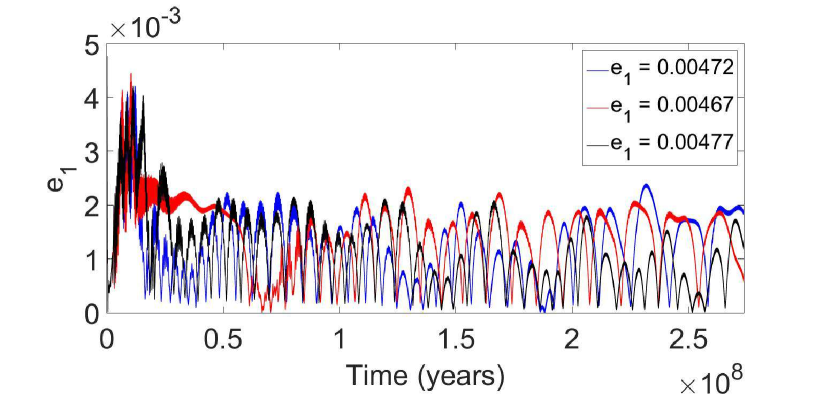
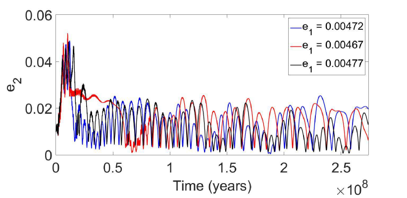
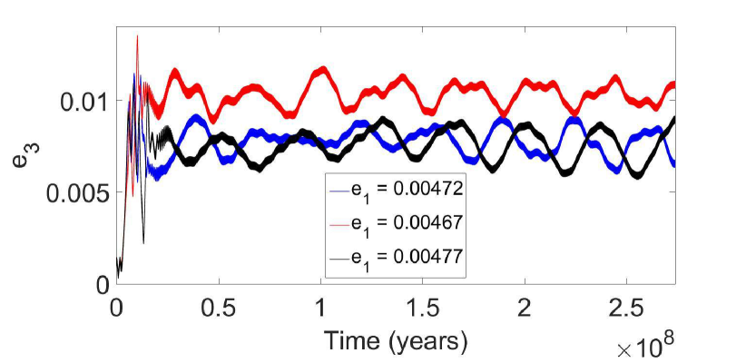
Figure 8: Evolution of the eccentricities of $S_{1}$ (top panel), $S_{2}$ (middle panel), and $S_{3}$ (bottom panel) from the dissipative model assuming 2:1&3:1 resonance and using three different initial values of the eccentricity of $S_{1}$ when the factor multiplying the tidal dissipation is $\alpha=10^{5}$. The different values of the eccentricity of $S_{1}$ are $e_{1}=0.00472$ (the nominal one), $e_{1}=0.00467,$ and $e_{1}=0.0477$

4 Phase-space geometry and linear stability

In this section, we focus on the geometry of the phase space and the linear stability in the vicinity of exact resonant solutions including the tidal effect. We limit our study to the planar case with focus on first- and second-order resonances. We work with the resonant variables provided in Table 1; we note that $(q_{7},q_{8},q_{9})$ are not considered because we consider the planar problem alone.

Let $H_{r}=H_{r}(\@vec{q},\@vec{Q})$ be the Hamiltonian (3) in resonant action-angle variables $\@vec{q}=(q_{1},\dots,q_{6})$, $\@vec{Q}=(Q_{1},\dots,Q_{6})$, with $\@vec{Q}$ being the conjugated actions obtained from a suitable generating function in the conservative problem. The dynamics in these variables is determined by the system of equations:

$$\dot{q}_{k} = \frac{\partial H_{r}}{\partial Q_{k}}\ ,\quad k=1\dots 6\ ,$$

$$\dot{Q}_{1} = \dot{P}_{1}=-\frac{\partial H_{r}}{\partial p_{1}}+\frac{dP_{1}}{dt}\bigg{|}_{T}$$

$$\dot{Q}_{k} = \dot{P}_{k}=-\frac{\partial H_{r}}{\partial p_{k}}\ ,\quad k=2,3\ ,$$

$$\dot{Q}_{k} = F_{k}(\@vec{q},\@vec{Q})\ .\quad k=4,5,6\ ,$$ (7)

where $\frac{dP_{1}}{dt}\big{|}_{T}$ denotes the counterpart of the dissipative contributions (4) or (6) expressed in modified Delaunay variables. The functions $F_{k}=F_{k}(\@vec{q},\@vec{Q})$ are defined for first-order resonances as listed below:

2:1 & 2:1:

$$F_{4} = \frac{1}{3}\left(2\dot{L}_{1}+\dot{L}_{2}-\dot{L}_{3}\right)\ ,$$

$$F_{5} = \frac{1}{3}\left(\dot{P}_{1}+\dot{P}_{2}+\dot{P}_{3}+3\dot{L}_{1}+\dot{L}_{2}\right)\ ,$$

$$F_{6} = \dot{L}_{1}+\dot{L}_{2}+\dot{L}_{3}-\dot{P}_{1}-\dot{P}_{2}-\dot{P}_{3}\ ,$$ (8)

2:1 & 3:2:

$$F_{4} = \frac{1}{4}\left(2\dot{P}_{1}+2\dot{P}_{2}-2\dot{P}_{3}-\dot{L}_{2}\right)\ ,$$

$$F_{5} = \frac{1}{4}\left(2\dot{P}_{1}+2\dot{P}_{2}+2\dot{P}_{3}+4\dot{L}_{1}+\dot{L}_{2}\right)\ ,$$

$$F_{6} = \dot{L}_{1}+\dot{L}_{2}+\dot{L}_{3}-\dot{P}_{1}-\dot{P}_{2}-\dot{P}_{3}\ .$$ (9)

3:2 & 3:2:

$$F_{4} = \frac{1}{5}\left(-3\dot{P}_{1}-3\dot{P}_{2}+2\dot{P}_{3}+\dot{L}_{2}\right)\ ,$$

$$F_{5} = \frac{1}{5}\left(4\dot{P}_{1}+4\dot{P}_{2}+4\dot{P}_{3}+5\dot{L}_{1}+2\dot{L}_{2}\right)\ ,$$

$$F_{6} = \dot{L}_{1}+\dot{L}_{2}+\dot{L}_{3}-\dot{P}_{1}-\dot{P}_{2}-\dot{P}_{3}\ .$$ (10)

In the above equations, (4) - (4), the derivatives $\dot{L}_{1}$, $\dot{L}_{2}$, $\dot{L}_{3}$, $\dot{P}_{1}$, $\dot{P}_{2}$, and $\dot{P}_{3}$ are obtained from the Hamiltonian flow, including the tidal effect on the first satellite:

$$\dot{L}_{1} = -\frac{\partial H_{r}}{\partial\lambda_{1}}+\frac{dL_{1}}{dt}\bigg{|}_{T}$$

$$\dot{L}_{k} = -\frac{\partial H_{r}}{\partial\lambda_{k}},\quad k=2,3\ ,$$

$$\dot{P}_{1} = -\frac{\partial H_{r}}{\partial p_{1}}+\frac{dP_{1}}{dt}\bigg{|}_{T},$$

$$\dot{P}_{k} = -\frac{\partial H_{r}}{\partial p_{k}}\ ,\quad k=2,3\ ,$$ (11)

where, again, $\frac{dL_{1}}{dt}\bigg{|}_{T}$ denotes the counterpart of the dissipative contributions (4) or (6) in the variables $(\lambda_{k},p_{k},L_{k},P_{k})$.

We remark that the derivatives of terms with respect to the modified Delaunay variables in Eqs. (4)-(4) have to be expressed in the suitable set of resonant variables (provided in Table 1). We also note that the resonant system, including the nonconservative terms, is again independent of the resonant angles $q_{5}$, $q_{6}$ because the nonconservative contributions only consist of secular terms that are independent of these variables, as in the conservative case. Thus, it suffices to investigate the reduced phase space $(q_{1},\dots,q_{4})$, $(Q_{1},\dots,Q_{4})$. However, we note that in presence of tides, the variables $Q_{5}$, $Q_{6}$ are not conserved quantities anymore, unless we solve for initial conditions with $\dot{Q}_{5}=\dot{Q}_{6}=0$, as is the case for fully resonant initial conditions.

4.1 Equilibria of the system and linear stability

An equilibrium of the vector field (4) in resonant variables is determined by the system of equations

$$\dot{q}_{1}=\dot{q}_{2}=\dot{q}_{3}=\dot{q}_{4}=\dot{Q}_{1}=\dot{Q}_{2}=\dot{Q}_{3}=\dot{Q}_{4}=\dot{Q}_{5}=\dot{Q}_{6}=0\ .$$ (12)

We solve it by using a root finding algorithm with the starting values close to the commensurability of the mean motions of the satellites. We remark that the additional conditions $\dot{Q}_{5}=\dot{Q}_{6}=0$ allow us to freeze the dynamics in phase space, which is done on purpose to reveal the structure of the phase space during capture, close to exact resonant conditions, that is, valid only for a frozen moment in time. We note that from a physical point of view, conditions (12) are never exactly fulfilled and $\dot{Q}_{5},\dot{Q}_{6}\neq 0$ in general.

Let $\@vec{q}^{\,*}=(q_{1}^{*},\dots,q_{4}^{*})$, ${\@vec{Q}}^{*}=(Q_{1}^{*},\dots,Q_{6}^{*})$ be quantities that solve Eq. (12) for fixed values of the system parameters. The equilibria (12) depend on i) the choice of the parameters (tidal effect, masses, etc.) and on ii) the choice of the resonant variables. In the following, we also investigate the effect of the system parameters on the linear stability indices at the equilibrium value for each resonance. If we denote the vector field (4) by

$$\dot{\@vec{X}}=\@vec{F}(\@vec{X}),$$ (13)

with the vector $\@vec{X}=(\@vec{q},\@vec{Q})$, the linear stability around the equilibrium $\@vec{X}^{*}=(\@vec{q}^{\,*},{\@vec{Q}}^{*})$ is given by the eigenvalues of the Jacobian matrix $\mathbf{J}$ evaluated at $\@vec{X}^{*}$,

$$\mathbf{J}=\left[\frac{\partial\@vec{F}}{\partial X_{1}}\dots\frac{\partial\@vec{F}}{\partial X_{12}}\right]\bigg{|}_{\@vec{X}=\@vec{X}^{*}}.$$ (14)

We evaluate $\mathbf{J}$ at the equilibrium $(\@vec{q}^{\,*},{\@vec{Q}}^{*})$ and determine numerically the eigenvalues for different system parameters. In the purely conservative case (without tides), we find complex conjugated eigenvalues, with zero real parts in all first-order resonant cases. Including the tidal effects, we find nonzero real parts due to the nonconservative effects.

We report projections of the phase space in the planes $(q_{1},Q_{1})$, $(q_{2},Q_{2})$, $(q_{3},Q_{3})$, and $(q_{4},Q_{4})$ in Figure 9 for the 2:1&2:1 resonant case. The equilibria coincide with $(\@vec{q}^{\,*},{\@vec{Q}}^{*})$ obtained from Eq. (12). Close to the equilibrium, the system oscillates around the centers with increasing amplitudes and increasing distance from $(\@vec{q}^{\,*},{\@vec{Q}}^{*})$.

To obtain the limiting librational curves (in red) in the projections $(q_{\ell},Q_{\ell})$, with $\ell=1,..,4$ we make use of the following iterative approach: we start by integrating sets of initial conditions with $(q_{k},Q_{k})=(q_{k}^{\,*},Q_{k}^{\,*})$ with $k=1,...,4$, $k\neq\ell$ and $q_{\ell}=q_{\ell}^{\,*}$, $Q_{\ell}=Q_{\ell}^{\,*}+\delta Q_{\ell}$ with one $\delta_{a}=\delta Q_{\ell}$ to obtain a librational curve and a second $\delta_{b}=\delta Q_{\ell}$ that yields a solution with $q_{\ell}\in[0,2\pi]$. Next we choose a fixed number of equally spaced initial conditions within the interval $\delta Q_{\ell}\in[\delta_{a},\delta_{b}]$ and keep at each iteration i) the largest $\delta Q_{\ell}$ that still yields librational motion and identify it with the new $\delta_{a}$, and ii) the smallest $\delta Q_{\ell}$ that still yields rotational motion and identify it with the new $\delta_{b}$. We iterate the process until $\delta_{b}-\delta_{a}$ becomes sufficiently small and define the librational half-width to be $\delta Q_{\ell}=\delta_{a}$. We note that this method yields a numerical estimate of the separatrix half-width in the plane $(q_{4},Q_{4})$, while for $\ell=1,2,3$ we obtainan estimate of the distance of the last paradoxal curve (see, e.g., Beaugé & Roig (2001)) that does not take all values from zero to $2\pi$.

4.2 Effect of tides and mass of $S_{1}$

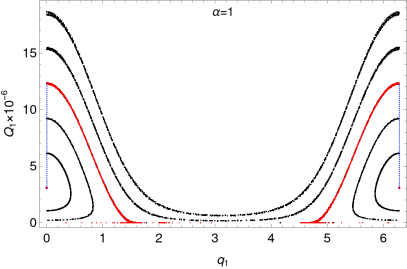
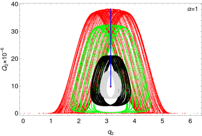
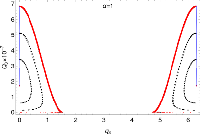
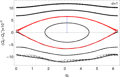
Figure 9: Projection of the phase space onto the plane $(q_{k},Q_{k})$ with $k=1,\dots,4$ for the 2:1&2:1 resonant case for $\alpha=1$. Equilibria, separatrix, and last paradoxal librational curve (see Beaugé & Roig (2001)) are shown in red, and the libration half-width is shown as a dotted blue line.

In order to reduce the integration time but at the same time observe the tidal effects for a long physical time, we multiply the variable $c$ in (5) by a factor $\alpha$. This technique is used in Showman & Malhotra (1997) and Lari et al. (2020), see also Celletti et al. (2021). We confirmed that the real parts of the eigenvalues, associated with Eq. (14), do not change sign with increasing value of $\alpha\in(1,10^{5})$. Moreover, we verified that the equilibria are only slightly shifted by magnification of the tidal effect. We conclude that a change in $\alpha$ does not change the topology of the phase space from a qualitative point of view.

The study to obtain the equilibria and stability indices was done for the 2:1&2:1, 2:1&3:2 and 3:2&3:2 resonant cases, taking the suitable resonant variables, see Table 1 and Eq. (4) for the definition of the functions $F_{4}$–$F_{6}$ in (4). We solve Eq. (12) for the equilibria ($\@vec{q}^{\,*},{\@vec{Q}}^{*}$) and make use of Eq. (14) to obtain the eigenvalues at equilibrium. We validate the results by a numerical integration of Eq. (4) for different initial conditions and also calculate the $\delta Q_{k}$ with $k=1,...,4$. The projections on the planes $(q_{1},Q_{1}),\dots,(q_{4},Q_{4})$ are similar to those of Figure 9 (not shown here).

We provide the results in phase space in dependence on the mass parameter of $S_{1}$. We repeat the study to solve Eq. (12) with varying values of $m_{1}$. The results are shown in Figure 10, where we report the shift in equilibrium value $Q_{4}^{*}$ versus the mass $m_{1}$ ranging from $0.5\ m_{1}$ to $5\ m_{1}$. We clearly see a dependence on the location of $Q_{4}^{*}$ in the projections of the phase space $(q_{4},Q_{4})$ with increasing mass of the innermost moon. We provide the study for case $\alpha=10^{0}$ (in blue) and $\alpha=10^{3}$ (in red), the shift following the same dependence on $m_{1}$ with slightly larger deviations from each other for lower masses of $S_{1}$.

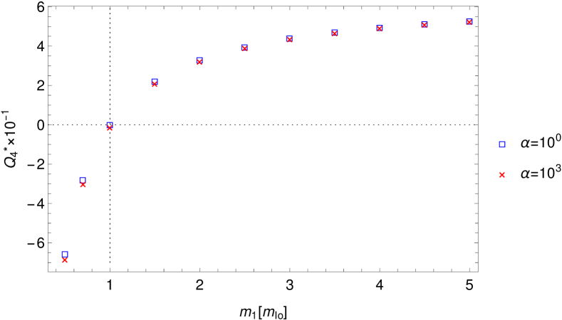
Figure 10: Equilibrium value $Q_{4}^{*}$ vs. $m_{1}$ (in units of Io’s mass) for different $\alpha$ (2:1&2:1 resonance). The reference values for the actual Galilean system are indicated by dashed lines.

We repeat the study for the 2:1&3:2 case. The results are shown in the top row of Figure 11. In the left panel of Figure 11 we see a comparable behavior of $Q_{4}^{*}$ with changing $m_{1}$ as for the 2:1&2:1 resonant case, but on different orders of magnitudes. The equilibrium $Q_{4}^{*}$ is shifted toward lower values for lower values of $m_{1}$, and higher if the mass of $S_{1}$ is increased.

Next, we investigate the width of the librational motions in dependence on the mass of $S_{1}$. The widths are defined as the distance $\delta Q_{k}$ from the equilibrium toward the last librational curve projected onto the planes, $(q_{k},Q_{k})$, found numerically by fixing the $(q_{\ell},Q_{\ell})$, and varying ${Q_{k}}^{*}$ with $k\neq\ell$ and $k=1,\dots,4$ (see end of Section 4.1 for more details). We clearly see that the librational widths decrease with increasing $m_{1}$ and keeping the order $\delta Q_{4}<\delta Q_{2}<\delta Q_{3}<\delta Q_{1}$. We remark that this result is of particular importance for understanding the capture probabilities that are also related to the width of the resonance in phase space. We conclude that for higher masses, the width (and capture probabilities) decreases.

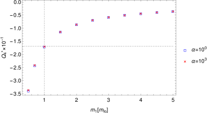
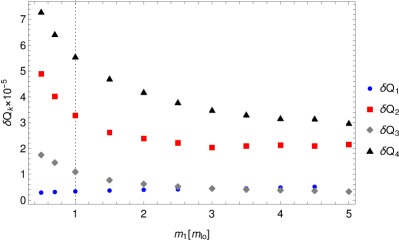
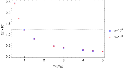
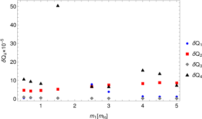
Figure 11: Equilibrium value $Q_{4}^{*}$ (left) and libration half-width $\delta Q_{1}$ … $\delta Q_{4}$ (right) vs. mass of $S_{1}$ - $m_{1}$ (in units of the mass of Io) for different $\alpha$ (left column). The top row refers to the 2:1&3:2 resonance, and the bottom row shows the 3:2&3:2 resonance. The reference values for the actual Galilean system are indicated by dashed lines.

We make a similar computation for the 3:2&3:2 resonance. The results are provided in the bottom row of Figure 11. We note the following difference in comparison with the 2:1&2:1 and 2:1&3:2 resonances: i) the equilibrium value of $Q_{\ell}$ decreases with increasing $m_{1}$ (numerical problems occur at $m_{1}=2$ and $m_{1}=3.5$ that are left out); ii) the separatrix half-widths change in a much more irregular way than in the previous cases. We stress that in this case, the dynamics is heavily affected by the mass $m_{1}$ in the sense that the evolution displays a chaotic behavior when $m_{1}$ increases.

The results shown in the bottom right panel of Figure 11 should therefore be seen with caution because the numerical method with which $\delta Q_{4}$ was obatained is strongly affected by the irregular behavior of the dynamics.

4.3 Higher-order resonances

We also performed similar calculations for the second- and mixed-order resonant cases. However, as already indicated by the numerical simulations in Section 3, the motion close to the exact resonant configuration becomes much more complex. In case of the second-order 3:1&3:1 resonance, when tides are incldued, we find complex conjugated pairs of eigenvalues with nonzero real parts. The librational half-widths for Galilean mass parameters are smaller by a factor 1-10 ($\delta Q_{1},\delta Q_{2}\propto 10^{-5}$, $\delta Q_{3}\propto 10^{-6}$), and $\delta Q_{4}\simeq 1.3-1.4\times 10^{-5}$ than for the first-order resonances, for which $\delta Q_{4}\simeq 7-10\times 10^{-5}$, for instance. Moreover, in addition to the reduced size of the resonant domain of motions, we also find a much stronger distortion of near resonant orbits when projected onto the $(q_{k},Q_{k}),\;k=1,\dots,4$ planes. As an example, we provide the projection of orbits onto the sections $(q_{3},Q_{3})$ (top) and $(q_{4},Q_{4})$ (bottom) plotted in Figure 12. We clearly observe that projections onto the plane $(q_{3},Q_{3})$ (for initial conditions starting at exact resonant values in the other planes) look quite regular, while deviations from exact resonant conditions in the plane $(q_{4},Q_{4})$ result in strongly perturbed orbits, where the resonant structure of the phase space is essentially destroyed. We notice that a series of numerical simulations revealed that the perturbations strongly depend on the mass ratio of the innermost two moons. For example, decreasing the mass of the second satellite by several orders of magnitudes results in less perturbed orbits. A similar phenomenon can be observed in the case of mixed-order resonances. If we repeat the study in the case of the 2:1&3:1 resonance, we find considerable distortions of the phase space close to the exact resonant configuration, which is strongly related to the mass of the second moon.

We note that more regular configurations of Laplace-like resonances may exist. However, a complete parameter study extended to cases with arbitrary mass ratios is beyond the scope of the current investigations. To conclude, trapping in mixed- and higher-order resonances could not be found for parameters close to the Galilean satellite system. The perturbations, mainly due to the second satellite, together with the reduced size of the librational regimes in phase space, are a possible explanation to justify the phenomenon found by pure numerical integrations. An analytical test of these results can be devised by computing resonant normal forms along the lines followed in Henrard (1984); Pucacco (2021) suitably extended to higher orders: a task for investigations in the near future.

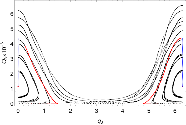
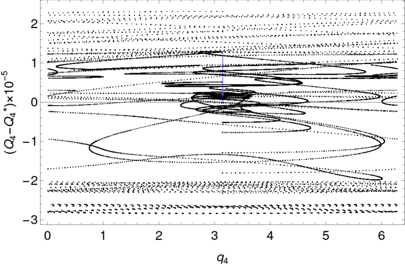
Figure 12: Strongly perturbed dynamics close to an equilibrium of the 3:1&3:1 resonance, projected onto the plane $(q_{3},Q_{3})$ (top) and $(q_{4},Q_{4}-{Q_{4}}^{*})$ (bottom).

5 Fate of the fourth satellite

In this section, we integrate numerically the equations of motion described in Section 2 including the tidal interaction between the central body and the first satellite for a long timescale. The numerical integrations of this section are perfomed using a program in C language that implements a Runge-Kutta fourth-order scheme with a fixed step size. The model was modified in order to include the mutual gravitational interactions due to the fourth satellite and not only the secular part. In this way, the possibility of a capture of $S_{4}$ is investigated in the case of the Laplace-like resonances. According to Lari et al. (2020), in the Galilean system, Callisto is captured into resonance with Ganymede after about 1.5 Gyr. Once again, the behavior of first- and second-order resonances is markedly different: in the cases of first-order resonances, $S_{4}$ is captured into resonance, while in mixed- and second-order resonances, this effect is not observed.

In the case of the 3:2&3:2 resonance, we note the capture of $S_{4}$ in a 2:1 resonance with $S_{3}$. We studied 100 different values for the initial mean longitude of $S_{4}$ , and in all the cases, the result was the same. The capture is obvious from the top panel of Figure 13, showing the ratio of the mean motions of $S_{3}$ and $S_{4}$. The resonant angle that involves the mean longitudes of the three outer satellites $S_{2}$, $S_{3}$ , and $S_{4}$, namely $2\lambda_{4}-4\lambda_{3}+2\lambda_{2}$, rotates at the beginning; after almost 1.2 Gyr, we note that this angle librates around $180^{\circ}$. The individual resonant angles $3\lambda_{3}-2\lambda_{2}-\omega_{3}$ and $2\lambda_{4}-\lambda_{3}-\omega_{3}$ rotate before and after the trapping of $S_{4}$ (bottom of Figure 13).

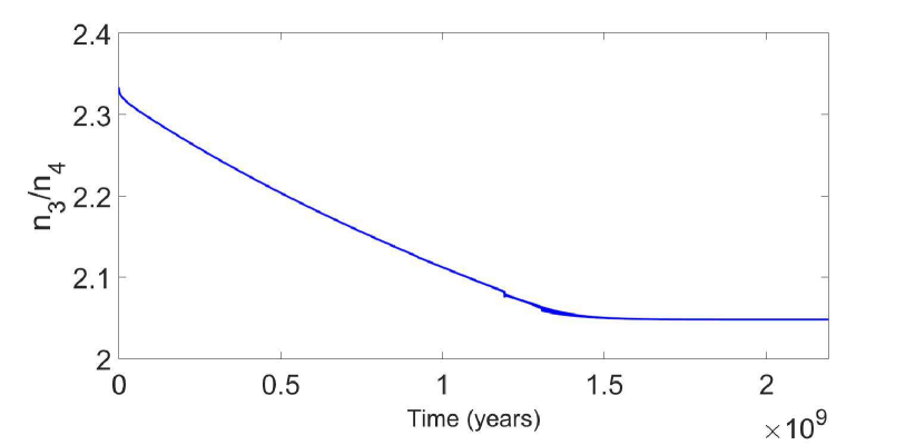
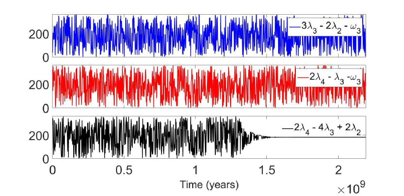
Figure 13: Evolution of the ratio of the mean motions of $S_{3}$ and $S_{4}$ (top panel) and the evolution of the resonant angles involving the mean longitudes of $S_{2}$, $S_{3}$ , and $S_{4}$ (bottom panel) in the case of the 3:2&3:2 resonance between the three innermost satellites, considering the tidal dissipation assuming a fast-rotating central body. The tidal effects are multiplied by a factor $\alpha=10^{4}$.

A similar behavior is observed for the 2:1&3:2 resonance testing 100 different initial values for the mean longitude of $S_{4}$. The difference between the two resonances is that in the 2:1&3:2 case, both the individual resonant angles and the angle that involves all three mean longitudes librate after the trapping of $S_{4}$.

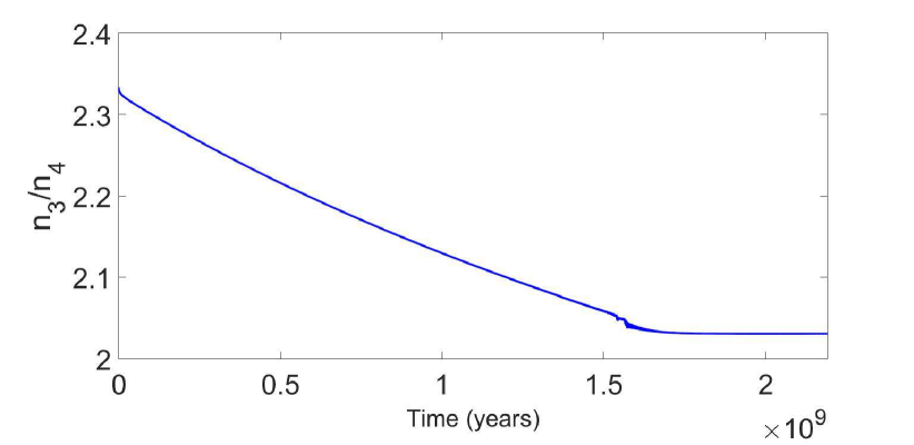
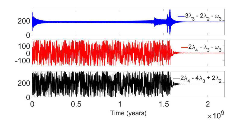
Figure 14: Evolution of the ratio of the mean motions of $S_{3}$ and $S_{4}$ (top panel) and the evolution of the resonant angles involving the mean longitudes of $S_{2}$, $S_{3}$ , and $S_{4}$ (bottom panel) in the case of the 2:1&3:2 resonance of the three innermost moons considering the tidal dissipation assuming a fast-rotating central body. The tidal effects are multiplied by a factor $10^{4}$.

6 Summary and conclusions

We studied Laplace-like resonances generalized to different commensurabilities in the frequencies of the orbital longitudes of three celestial bodies that revolve around a central body, and investigated the possibility of capture of a fourth body in resonant configuration with the other three bodies. Our model includes the mutual gravitational interaction of the celestial bodies, the secular effects of oblateness, and a distant star such as the Sun, as well as the tidal effect on the innermost celestial body close to the central body. A typical application of this model is the Galilean satellite system of planet Jupiter, where Io, Europa, and Ganymede are already found in a 2:1&2:1 resonant configuration, and the moon Callisto may be trapped in resonance with these moons in future times. The outcome of this system during the formation of the Solar System may have been different, that is, the three moons may have been in different resonant configurations. In addition, the results of our study may be applied to other planetary moon systems.

From the numerical integrations performed in this work, a significant difference between the first-, second- and mixed-order resonances can be highlighted. Under the tidal effects between the central body and the innermost body, the three inner satellites move outward in the case of first-order resonances. In the second- and mixed-order resonances, the evolution of the system is different, and only the closest or the two closest satellites move outward, respectively. Moreover, the resonant angle that involves the mean longitudes of the three inner bodies librates only in the first-order resonances, but circulates in the remaining resonances.

The evolution of a satellite system is dominated by the tidal interaction of the central body and the innermost satellite. However, the rotation of the central body plays a crucial role in the evolution of the orbital elements of the satellites. While in the case of the fast-rotating central body, the resonant arguments librate in first-order resonances and circulate in mixed- and second-order resonances, when a slowly rotating central body is assumed, the resonant arguments circulate.

Moreover, the geometry of the phase space of the first-order resonances was studied. The system oscillates around the equilibria, and the separatrix and last paradoxal librational curve were computed. The computation of the equilibrium values and especially ${Q_{4}}^{*}$ was performed using different values of the mass of the innermost satellite pointing out the dependence on this parameter. Specifically, the maximum value of the eigenvalues decreases in magnitude as the value of $m_{1}$ increases.

Finally, the possibility of capture of the fourth satellite was studied in the case of first-order resonances. In the two first-order resonances we included, the fourth satellite is captured into resonance using 100 different values for the initial mean longitude of the fourth satellite. In the 3:2&3:2 resonance, the system develops two three-body resonances, a 3:2&3:2 among the inner three satellites and a 3:2&2:1 resonance among $S_{2}$, $S_{3}$ and $S_{4}$. In the 2:1&3:2 resonance, a chain of two-body resonances 2:1, 3:2, and 2:1 develops. This effect is not observed in the mixed- and second-order resonances.

Appendix A Hamiltonian function of the secular and resonant parts of the mutual satellite interactions

The secular and resonant parts of the Hamiltonian that we used to model the mutual interaction of the satellites for the 3:2&3:2 resonance are given by

$$H_{P}^{1,2} =-{\frac{Gm_{1}m_{2}}{a_{2}}}\big{(}B_{0}(\alpha_{1,2})$$

$$+{f_{A}}_{1}^{1,2}({e_{1}}^{2}+{e_{2}}^{2})$$

$$+{f_{A}}_{2}^{1,2}e_{1}\cos(3\lambda_{2}-2\lambda_{1}-\varpi_{1})$$

$$+{f_{A}}_{3}^{1,2}e_{2}\cos(3\lambda_{2}-2\lambda_{1}-\varpi_{2})$$

$$+{f_{A}}_{4}^{1,2}{e_{1}}^{2}\cos(6\lambda_{2}-4\lambda_{1}-2\varpi_{1})$$

$$+{f_{A}}_{5}^{1,2}{e_{2}}^{2}\cos(6\lambda_{2}-4\lambda_{1}-2\varpi_{2})$$

$$+{f_{A}}_{6}^{1,2}e_{1}e_{2}\cos(6\lambda_{2}-4\lambda_{1}-\varpi_{1}-\varpi_{2})$$

$$+{f_{A}}_{7}^{1,2}e_{1}e_{2}\cos(\varpi_{2}-\varpi_{1})$$

$$+{f_{A}}_{8}^{1,2}{s_{1}}^{2}\cos(6\lambda_{2}-4\lambda_{1}-2\Omega_{1})$$

$$+{f_{A}}_{9}^{1,2}{s_{2}}^{2}\cos(6\lambda_{2}-4\lambda_{1}-2\Omega_{2})$$

$$+{f_{A}}_{10}^{1,2}{s_{1}}{s_{2}}\cos(6\lambda_{2}-4\lambda_{1}-\Omega_{1}-\Omega_{2})$$

$$+{f_{A}}_{11}^{1,2}{s_{1}}{s_{2}}\cos(\Omega_{1}-\Omega_{2})\big{)}$$

$$H_{P}^{2,3} =-{\frac{Gm_{2}m_{3}}{a_{3}}}\big{(}B_{0}(\alpha_{2,3})$$

$$+{f_{A}}_{1}^{2,3}({e_{2}}^{2}+{e_{3}}^{2})$$

$$+{f_{A}}_{2}^{2,3}e_{2}\cos(3\lambda_{3}-2\lambda_{2}-\varpi_{2})$$

$$+{f_{A}}_{3}^{2,3}e_{3}\cos(3\lambda_{3}-2\lambda_{2}-\varpi_{3})$$

$$+{f_{A}}_{4}^{2,3}{e_{2}}^{2}\cos(6\lambda_{3}-4\lambda_{2}-2\varpi_{2})$$

$$+{f_{A}}_{5}^{2,3}{e_{3}}^{2}\cos(6\lambda_{3}-4\lambda_{2}-2\varpi_{3})$$

$$+{f_{A}}_{6}^{2,3}e_{2}e_{3}\cos(6\lambda_{3}-4\lambda_{2}-\varpi_{2}-\varpi_{3})$$

$$+{f_{A}}_{7}^{2,3}e_{2}e_{3}\cos(\varpi_{3}-\varpi_{2})$$

$$+{f_{A}}_{8}^{2,3}{s_{2}}^{2}\cos(6\lambda_{3}-4\lambda_{2}-2\Omega_{2})$$

$$+{f_{A}}_{9}^{2,3}{s_{3}}^{2}\cos(6\lambda_{3}-4\lambda_{2}-2\Omega_{3})$$

$$+{f_{A}}_{10}^{2,3}{s_{2}}{s_{3}}\cos(6\lambda_{3}-4\lambda_{2}-\Omega_{2}-\Omega_{3})$$

$$+{f_{A}}_{11}^{2,3}{s_{2}}{s_{3}}\cos(\Omega_{2}-\Omega_{3})\big{)}$$

$$H_{P}^{1,3} =-{\frac{Gm_{1}m_{3}}{a_{3}}}\big{(}B_{0}(\alpha_{1,3})$$

$$+{f_{A}}_{1}^{1,3}(e_{1}^{2}+e_{3}^{2})$$

$$+{f_{A}}_{7}^{1,3}e_{1}e_{3}\cos(\varpi_{3}-\varpi_{1})$$

$$+{f_{A}}_{11}^{1,3}{s_{1}}{s_{3}}\cos(\Omega_{1}-\Omega_{3})\big{)}\ .$$

The resonant part of the Hamiltonian that corresponds to the 2:1&3:2 resonance is given by

$$H_{P}^{1,2} =-{{Gm_{1}m_{2}}\over a_{2}}\big{(}B_{0}(\alpha_{1,2})$$

$$+{f_{B}}_{1}^{1,2}({e_{1}}^{2}+{e_{2}}^{2})$$

$$+{f_{B}}_{2}^{1,2}e_{1}\cos(2\lambda_{2}-\lambda_{1}-\varpi_{1})$$

$$+{f_{B}}_{3}^{1,2}e_{2}\cos(2\lambda_{2}-\lambda_{1}-\varpi_{2})$$

$$+{f_{B}}_{4}^{1,2}{e_{1}}^{2}\cos(4\lambda_{2}-2\lambda_{1}-2\varpi_{1})$$

$$+{f_{B}}_{5}^{1,2}{e_{2}}^{2}\cos(4\lambda_{2}-2\lambda_{1}-2\varpi_{2})$$

$$+{f_{B}}_{6}^{1,2}e_{1}e_{2}\cos(4\lambda_{2}-2\lambda_{1}-\varpi_{1}-\varpi_{2})$$

$$+{f_{B}}_{7}^{1,2}e_{1}e_{2}\cos(\varpi_{2}-\varpi_{1})$$

$$+{f_{B}}_{8}^{1,2}{s_{1}}^{2}\cos(4\lambda_{2}-2\lambda_{1}-2\Omega_{1})$$

$$+{f_{B}}_{9}^{1,2}{s_{2}}^{2}\cos(4\lambda_{2}-2\lambda_{1}-2\Omega_{2})$$

$$+{f_{B}}_{10}^{1,2}{s_{1}}{s_{2}}\cos(4\lambda_{2}-2\lambda_{1}-\Omega_{1}-\Omega_{2})$$

$$+{f_{B}}_{11}^{1,2}{s_{1}}{s_{2}}\cos(\Omega_{1}-\Omega_{2})\big{)}$$

$$H_{P}^{2,3} =-{{Gm_{2}m_{3}}\over a_{3}}\big{(}B_{0}(\alpha_{2,3})$$

$$+{f_{A}}_{1}^{2,3}({e_{2}}^{2}+{e_{3}}^{2})$$

$$+{f_{A}}_{2}^{2,3}e_{2}\cos(3\lambda_{3}-2\lambda_{2}-\varpi_{2})$$

$$+{f_{A}}_{3}^{2,3}e_{3}\cos(3\lambda_{3}-2\lambda_{2}-\varpi_{3})$$

$$+{f_{A}}_{4}^{2,3}{e_{2}}^{2}\cos(6\lambda_{3}-4\lambda_{2}-2\varpi_{2})$$

$$+{f_{A}}_{5}^{2,3}{e_{3}}^{2}\cos(6\lambda_{3}-4\lambda_{2}-2\varpi_{3})$$

$$+{f_{A}}_{6}^{2,3}e_{2}e_{3}\cos(6\lambda_{3}-4\lambda_{2}-\varpi_{2}-\varpi_{3})$$

$$+{f_{A}}_{7}^{2,3}e_{2}e_{3}\cos(\varpi_{3}-\varpi_{2})$$

$$+{f_{A}}_{8}^{2,3}{s_{2}}^{2}\cos(6\lambda_{3}-4\lambda_{2}-2\Omega_{2})$$

$$+{f_{A}}_{9}^{2,3}{s_{3}}^{2}\cos(6\lambda_{3}-4\lambda_{2}-2\Omega_{3})$$

$$+{f_{A}}_{10}^{2,3}{s_{2}}{s_{3}}\cos(6\lambda_{3}-4\lambda_{2}-\Omega_{2}-\Omega_{3})$$

$$+{f_{A}}_{11}^{2,3}{s_{2}}{s_{3}}\cos(\Omega_{2}-\Omega_{3})\big{)}$$

$$H_{P}^{1,3} =-{{Gm_{1}m_{3}}\over a_{3}}\big{(}B_{0}(\alpha_{1,3})$$

$$+{f_{A}}_{1}^{1,3}(e_{1}^{2}+e_{3}^{2})$$

$$+{f_{A}}_{7}^{1,3}e_{1}e_{3}\cos(\varpi_{3}-\varpi_{1})$$

$$+{f_{A}}_{11}^{1,3}{s_{1}}{s_{3}}\cos(\Omega_{1}-\Omega_{3})\big{)}\ .$$

The resonant part of the Hamiltonian that corresponds to the 3:1&3:1 resonance is given by

$$H_{P}^{1,2}=-{{Gm_{1}m_{2}}\over a_{2}}\big{(}B_{0}(\alpha_{1,2})$$

$$+{f_{C}}_{1}^{1,2}({e_{1}}^{2}+{e_{2}}^{2})$$

$$+{f_{C}}_{2}^{1,2}{e_{1}}^{2}\cos(3\lambda_{2}-\lambda_{1}-2\varpi_{1})$$

$$+{f_{C}}_{3}^{1,2}e_{1}e_{2}\cos(3\lambda_{2}-\lambda_{1}-\varpi_{1}-\varpi_{2})$$

$$+{f_{C}}_{4}^{1,2}{e_{2}}^{2}\cos(3\lambda_{2}-\lambda_{1}-2\varpi_{2})$$

$$+{f_{C}}_{5}^{1,2}e_{1}e_{2}\cos(\varpi_{2}-\varpi_{1})$$

$$+{f_{C}}_{6}^{1,2}{s_{1}}^{2}\cos(3\lambda_{2}-\lambda_{1}-2\Omega_{1})$$

$$+{f_{C}}_{7}^{1,2}s_{1}s_{2}\cos(3\lambda_{2}-\lambda_{1}-\Omega_{1}-\Omega_{2})$$

$$+{f_{C}}_{8}^{1,2}{s_{2}}^{2}\cos(3\lambda_{2}-\lambda_{1}-2\Omega_{2})$$

$$+{f_{C}}_{9}^{1,2}s_{1}s_{2}\cos(\Omega_{2}-\Omega_{1})\big{)}$$

$$H_{P}^{2,3} =-{{Gm_{2}m_{3}}\over a_{3}}\big{(}B_{0}(\alpha_{2,3})$$

$$+{f_{C}}_{1}^{2,3}({e_{2}}^{2}+{e_{3}}^{2})$$

$$+{f_{C}}_{2}^{2,3}{e_{2}}^{2}\cos(3\lambda_{3}-\lambda_{2}-2\varpi_{2})$$

$$+{f_{C}}_{3}^{2,1}e_{2}e_{3}\cos(3\lambda_{3}-\lambda_{2}-\varpi_{2}-\varpi_{3})$$

$$+{f_{C}}_{4}^{2,3}{e_{3}}^{2}\cos(3\lambda_{3}-\lambda_{2}-2\varpi_{3})$$

$$+{f_{C}}_{5}^{2,3}e_{2}e_{3}\cos(\varpi_{3}-\varpi_{2})$$

$$+{f_{C}}_{6}^{2,3}{s_{2}}^{2}\cos(3\lambda_{3}-\lambda_{2}-2\Omega_{2})$$

$$+{f_{C}}_{7}^{2,1}s_{2}s_{3}\cos(3\lambda_{3}-\lambda_{2}-\Omega_{2}-\Omega_{3})$$

$$+{f_{C}}_{8}^{2,3}{s_{3}}^{2}\cos(3\lambda_{3}-\lambda_{2}-2\Omega_{3})$$

$$+{f_{C}}_{9}^{2,3}s_{2}s_{3}\cos(\Omega_{3}-\Omega_{2})\big{)}$$

$$H_{P}^{1,3} =-{{Gm_{1}m_{3}}\over a_{3}}\big{(}B_{0}(\alpha_{1,3})$$

$$+{f_{C}}_{1}^{1,3}(e_{1}^{2}+e_{3}^{2})$$

$$+{f_{C}}_{5}^{1,3}e_{1}e_{3}\cos(\varpi_{3}-\varpi_{1})$$

$$+{f_{C}}_{9}^{1,3}s_{1}s_{3}\cos(\Omega_{3}-\Omega_{1})\big{)}\ .$$

The resonant part of the Hamiltonian that corresponds to the 2:1&3:1 resonance is given by

$$H_{P}^{1,2} =-{{Gm_{1}m_{2}}\over a_{2}}\big{(}B_{0}(\alpha_{1,2})$$

$$+{f_{B}}_{1}^{1,2}({e_{1}}^{2}+{e_{2}}^{2})$$

$$+{f_{B}}_{2}^{1,2}e_{1}\cos(2\lambda_{2}-\lambda_{1}-\varpi_{1})$$

$$+{f_{B}}_{3}^{1,2}e_{2}\cos(2\lambda_{2}-\lambda_{1}-\varpi_{2})$$

$$+{f_{B}}_{4}^{1,2}{e_{1}}^{2}\cos(4\lambda_{2}-2\lambda_{1}-2\varpi_{1})$$

$$+{f_{B}}_{5}^{1,2}{e_{2}}^{2}\cos(4\lambda_{2}-2\lambda_{1}-2\varpi_{2})$$

$$+{f_{B}}_{6}^{1,2}e_{1}e_{2}\cos(4\lambda_{2}-2\lambda_{1}-\varpi_{1}-\varpi_{2})$$

$$+{f_{B}}_{7}^{1,2}e_{1}e_{2}\cos(\varpi_{2}-\varpi_{1})$$

$$+{f_{B}}_{8}^{1,2}{s_{1}}^{2}\cos(4\lambda_{2}-2\lambda_{1}-2\Omega_{1})$$

$$+{f_{B}}_{9}^{1,2}{s_{2}}^{2}\cos(4\lambda_{2}-2\lambda_{1}-2\Omega_{2})$$

$$+{f_{B}}_{10}^{1,2}{s_{1}}{s_{2}}\cos(4\lambda_{2}-2\lambda_{1}-\Omega_{1}-\Omega_{2})$$

$$+{f_{B}}_{11}^{1,2}{s_{1}}{s_{2}}\cos(\Omega_{1}-\Omega_{2})\big{)}$$

$$H_{P}^{2,3} =-{{Gm_{2}m_{3}}\over a_{3}}\big{(}B_{0}(\alpha_{2,3})$$

$$+{f_{C}}_{1}^{2,3}({e_{2}}^{2}+{e_{3}}^{2})$$

$$+{f_{C}}_{2}^{2,3}{e_{2}}^{2}\cos(3\lambda_{3}-\lambda_{2}-2\varpi_{2})$$

$$+{f_{C}}_{3}^{2,1}e_{2}e_{3}\cos(3\lambda_{3}-\lambda_{2}-\varpi_{2}-\varpi_{3})$$

$$+{f_{C}}_{4}^{2,3}{e_{3}}^{2}\cos(3\lambda_{3}-\lambda_{2}-2\varpi_{3})$$

$$+{f_{C}}_{5}^{2,3}e_{2}e_{3}\cos(\varpi_{3}-\varpi_{2})$$

$$+{f_{C}}_{6}^{2,3}{s_{2}}^{2}\cos(3\lambda_{3}-\lambda_{2}-2\Omega_{2})$$

$$+{f_{C}}_{7}^{2,1}s_{2}s_{3}\cos(3\lambda_{3}-\lambda_{2}-\Omega_{2}-\Omega_{3})$$

$$+{f_{C}}_{8}^{2,3}{s_{3}}^{2}\cos(3\lambda_{3}-\lambda_{2}-2\Omega_{3})$$

$$+{f_{C}}_{9}^{2,3}s_{2}s_{3}\cos(\Omega_{3}-\Omega_{2})\big{)}$$

$$H_{P}^{1,3} =-{{Gm_{1}m_{3}}\over a_{3}}\big{(}B_{0}(\alpha_{1,3})$$

$$+{f_{C}}_{1}^{1,3}(e_{1}^{2}+e_{3}^{2})$$

$$+{f_{C}}_{5}^{1,3}e_{1}e_{3}\cos(\varpi_{3}-\varpi_{1})$$

$$+{f_{C}}_{9}^{1,3}s_{1}s_{3}\cos(\Omega_{3}-\Omega_{1})\big{)}\ .$$

In these expressions, $\alpha_{ij}=\frac{a_{i}}{a_{j}}$ is the ratio of the semimajor axes of the $i$-th and $j$-th satellite, $B_{0}(\alpha_{i,j})=\frac{1}{2}{b_{1/2}}^{(0)}(\alpha_{i,j})-1$, and the functions ${f_{Ak}}^{i,j}$, ${f_{Bk}}^{i,j}$, ${f_{Ck}}^{i,j}$ are linear combinations of the Laplace coefficients ${b_{s}}^{(n)}$ and their derivatives (Murray & Dermott (1999), Ellis & Murray (2000), Celletti et al. (2019)), as given below:

$${f_{A1}}^{i,j}=\bigg{(}\frac{1}{4}\alpha_{i,j}\frac{d}{d\alpha_{i,j}}+\frac{1}{8}{\alpha_{i,j}}^{2}\frac{d^{2}}{{d\alpha_{i,j}}^{2}}\bigg{)}{b_{1/2}}^{(0)}(\alpha_{i,j})$$

$${f_{A2}}^{i,j}=-3{b_{1/2}}^{(3)}(\alpha_{i,j})+\frac{1}{2}\alpha_{i,j}\frac{d}{d\alpha_{i,j}}{b_{1/2}}^{(3)}(\alpha_{i,j})$$

$${f_{A3}}^{i,j}=\frac{5}{2}{b_{1/2}}^{(2)}(\alpha_{i,j})+\frac{1}{2}\alpha_{i,j}\frac{d}{d\alpha_{i,j}}{b_{1/2}}^{(2)}(\alpha_{i,j})$$

$${f_{A4}}^{i,j}= \frac{1}{8}\bigg{[}114{b_{1/2}}^{(6)}(\alpha_{i,j})+22\alpha_{i,j}\frac{d}{d\alpha_{i,j}}{b_{1/2}}^{(6)}(\alpha_{i,j})$$

$$+{\alpha_{i,j}}^{2}\frac{d^{2}}{d\alpha_{i,j}^{2}}{b_{1/2}}^{(6)}(\alpha_{i,j})\bigg{]}$$

$${f_{A5}}^{i,j}= \frac{1}{8}\bigg{[}104{b_{1/2}}^{(4)}(\alpha_{i,j})+22\alpha_{i,j}\frac{d}{d\alpha_{i,j}}{b_{1/2}}^{(4)}(\alpha_{i,j})$$

$$+{\alpha_{i,j}}^{2}\frac{d^{2}}{d\alpha_{i,j}^{2}}{b_{1/2}}^{(4)}(\alpha_{i,j})\bigg{]}$$

$${f_{A6}}^{i,j}= \frac{1}{4}\bigg{[}110{b_{1/2}}^{(5)}(\alpha_{i,j})+22\alpha_{i,j}\frac{d}{d\alpha_{i,j}}{b_{1/2}}^{(5)}(\alpha_{i,j})$$

$$+{\alpha_{i,j}}^{2}\frac{d^{2}}{d\alpha_{i,j}^{2}}{b_{1/2}}^{(5)}(\alpha_{i,j})\bigg{]}$$

$${f_{A7}}^{i,j}= \frac{1}{4}\bigg{[}2{b_{1/2}}^{(1)}(\alpha_{i,j})-2\alpha_{i,j}\frac{d}{d\alpha_{i,j}}{b_{1/2}}^{(1)}(\alpha_{i,j})$$

$$-{\alpha_{i,j}}^{2}\frac{d^{2}}{d\alpha_{i,j}^{2}}{b_{1/2}}^{(1)}(\alpha_{i,j})\bigg{]}$$

$${f_{A8}}^{i,j}=\frac{1}{2}\alpha_{i,j}{b_{3/2}}^{(5)}(\alpha_{i,j})$$

$${f_{A9}}^{i,j}=\frac{1}{2}\alpha_{i,j}{b_{3/2}}^{(5)}(\alpha_{i,j})$$

$${f_{A10}}^{i,j}=-\alpha_{i,j}{b_{3/2}}^{(5)}(\alpha_{i,j})$$

$${f_{A11}}^{i,j}=\alpha_{i,j}{b_{3/2}}^{(1)}(\alpha_{i,j})$$

$${f_{B1}}^{i,j}=\bigg{(}\frac{1}{4}\alpha_{i,j}\frac{d}{d\alpha_{i,j}}+\frac{1}{8}{\alpha_{i,j}}^{2}\frac{d^{2}}{{d\alpha_{i,j}}^{2}}\bigg{)}{b_{1/2}}^{(0)}(\alpha_{i,j})$$

$${f_{B2}}^{i,j}=-2{b_{1/2}}^{(2)}(\alpha_{i,j})+\frac{1}{2}\alpha_{i,j}\frac{d}{d\alpha_{i,j}}{b_{1/2}}^{(2)}(\alpha_{i,j})$$

$${f_{B3}}^{i,j}=\frac{3}{2}{b_{1/2}}^{(1)}(\alpha_{i,j})+\frac{1}{2}\alpha_{i,j}\frac{d}{d\alpha_{i,j}}{b_{1/2}}^{(1)}(\alpha_{i,j})-2\alpha_{i,j}$$

$${f_{B4}}^{i,j}= \frac{1}{8}\bigg{[}44{b_{1/2}}^{(4)}(\alpha_{i,j})+14\alpha_{i,j}\frac{d}{d\alpha_{i,j}}{b_{1/2}}^{(4)}(\alpha_{i,j})$$

$$+{\alpha_{i,j}}^{2}\frac{d^{2}}{d\alpha_{i,j}^{2}}{b_{1/2}}^{(4)}(\alpha_{i,j})\bigg{]}$$

$${f_{B5}}^{i,j}= \frac{1}{8}\bigg{[}38{b_{1/2}}^{(2)}(\alpha_{i,j})+14\alpha_{i,j}\frac{d}{d\alpha_{i,j}}{b_{1/2}}^{(2)}(\alpha_{i,j})$$

$$+{\alpha_{i,j}}^{2}\frac{d^{2}}{d\alpha_{i,j}^{2}}{b_{1/2}}^{(2)}(\alpha_{i,j})\bigg{]}$$

$${f_{B6}}^{i,j}= -\frac{1}{4}\bigg{[}42{b_{1/2}}^{(3)}(\alpha_{i,j})+14\alpha_{i,j}\frac{d}{d\alpha_{i,j}}{b_{1/2}}^{(3)}(\alpha_{i,j})$$

$$+{\alpha_{i,j}}^{2}\frac{d^{2}}{d\alpha_{i,j}^{2}}{b_{1/2}}^{(3)}(\alpha_{i,j})\bigg{]}$$

$${f_{B7}}^{i,j}= \frac{1}{4}\bigg{[}2{b_{1/2}}^{(1)}(\alpha_{i,j})-2\alpha_{i,j}\frac{d}{d\alpha_{i,j}}{b_{1/2}}^{(1)}(\alpha_{i,j})$$

$$-{\alpha_{i,j}}^{2}\frac{d^{2}}{d\alpha_{i,j}^{2}}{b_{1/2}}^{(1)}(\alpha_{i,j})\bigg{]}$$

$${f_{B8}}^{i,j}=\frac{1}{2}\alpha_{i,j}{b_{3/2}}^{(5)}(\alpha_{i,j})$$

$${f_{B9}}^{i,j}=\frac{1}{2}\alpha_{i,j}{b_{3/2}}^{(5)}(\alpha_{i,j})$$

$${f_{B10}}^{i,j}=-\alpha_{i,j}{b_{3/2}}^{(5)}(\alpha_{i,j})$$

$${f_{B11}}^{i,j}=\alpha_{i,j}{b_{3/2}}^{(1)}(\alpha_{i,j})$$

$${f_{C1}}^{i,j}=\bigg{(}\frac{1}{4}\alpha_{i,j}\frac{d}{d\alpha_{i,j}}+\frac{1}{8}{\alpha_{i,j}}^{2}\frac{d^{2}}{{d\alpha_{i,j}}^{2}}\bigg{)}{b_{1/2}}^{(0)}(\alpha_{i,j})$$

$${f_{C2}}^{i,j}= \frac{1}{8}\bigg{[}21{b_{1/2}}^{(3)}(\alpha_{i,j})+10\alpha_{i,j}\frac{d}{d\alpha_{i,j}}{b_{1/2}}^{(3)}(\alpha_{i,j})$$

$$+{\alpha_{i,j}}^{2}\frac{d^{2}}{d\alpha_{i,j}^{2}}{b_{1/2}}^{(3)}(\alpha_{i,j})\bigg{]}$$

$${f_{C3}}^{i,j}= \frac{1}{4}\bigg{[}-20{b_{1/2}}^{(2)}(\alpha_{i,j})-10\alpha_{i,j}\frac{d}{d\alpha_{i,j}}{b_{1/2}}^{(2)}(\alpha_{i,j})$$

$$-{\alpha_{i,j}}^{2}\frac{d^{2}}{d\alpha_{i,j}^{2}}{b_{1/2}}^{(2)}(\alpha_{i,j})\bigg{]}$$

$${f_{C4}}^{i,j}= \frac{1}{8}\bigg{[}17{b_{1/2}}^{(1)}(\alpha_{i,j})+10\alpha_{i,j}\frac{d}{d\alpha_{i,j}}{b_{1/2}}^{(1)}(\alpha_{i,j})$$

$$+{\alpha_{i,j}}^{2}\frac{d^{2}}{d\alpha_{i,j}^{2}}{b_{1/2}}^{(1)}(\alpha_{i,j})\bigg{]}-\frac{27}{8}\alpha_{i,j}$$

$${f_{C5}}^{i,j}= \frac{1}{4}\bigg{[}2{b_{1/2}}^{(1)}(\alpha_{i,j})-2\alpha_{i,j}\frac{d}{d\alpha_{i,j}}{b_{1/2}}^{(1)}(\alpha_{i,j})$$

$$-{\alpha_{i,j}}^{2}\frac{d^{2}}{d\alpha_{i,j}^{2}}{b_{1/2}}^{(1)}(\alpha_{i,j})\bigg{]}$$

$${f_{C6}}^{i,j}=\frac{1}{2}\alpha_{i,j}{b_{3/2}}^{(2)}(\alpha_{i,j})$$

$${f_{C7}}^{i,j}=\frac{1}{2}\alpha_{i,j}{b_{3/2}}^{(2)}(\alpha_{i,j})$$

$${f_{C8}}^{i,j}=-\alpha_{i,j}{b_{3/2}}^{(2)}(\alpha_{i,j})$$

$${f_{C9}}^{i,j}=\alpha_{i,j}{b_{3/2}}^{(1)}(\alpha_{i,j}).$$

References

• Beaugé & Roig (2001) Beaugé, C. & Roig, F. 2001, Icarus, 153, 391
• Celletti et al. (2021) Celletti, A., Karampotsiou, E., Lhotka, C., Pucacco, G., & Volpi, M. 2021, Preprint
• Celletti et al. (2019) Celletti, A., Paita, F., & Pucacco, G. 2019, Chaos, 29, 033111
• Christiansen et al. (2018) Christiansen, J. L., Crossfield, I. J., Barentsen, G., et al. 2018, AJ, 155, 57
• David et al. (2019) David, T. J., Petigura, E. A., & Luger, R. e. 2019, ApJ, 885, L12
• de Sitter (1928) de Sitter, W. 1928, Annalen van de Sterrewacht te Leiden, 16, B1
• Delisle (2017) Delisle, J. B. 2017, A&A, 605, A96
• Ellis & Murray (2000) Ellis, K. M. & Murray, C. D. 2000, Icarus, 147, 129
• Ferraz-Mello (1979) Ferraz-Mello, S. 1979, CEP, 5508, 090
• Ferraz-Mello et al. (2008) Ferraz-Mello, S., Rodríguez, A., & Hussmann, H. 2008, Celestial Mechanics and Dynamical Astronomy, 101, 171
• Hara et al. (2020) Hara, N., Bouchy, F., Stalport, M., et al. 2020, Astronomy & Astrophysics, 636, L6
• Henrard (1984) Henrard, J. 1984, Celestial Mechanics, 34, 255
• Lainey et al. (2009) Lainey, V., Arlot, J.-E., Karatekin, Ö., & Van Hoolst, T. 2009, Nature, 459, 957
• Lari et al. (2020) Lari, G., Saillenfest, M., & Fenucci, M. 2020, Astronomy & Astrophysics, 639, A40
• Lieske (1998) Lieske, J. 1998, Astronomy and Astrophysics Supplement Series, 129, 205
• Luger et al. (2017) Luger, R., Sestovic, M., Kruse, E., et al. 2017, Nature Astronomy, 1, 1
• Malhotra (1991) Malhotra, R. 1991, Icarus, 94, 399
• Murray & Dermott (1999) Murray, C. D. & Dermott, S. F. 1999, Solar system dynamics (Cambridge university press)
• Paita et al. (2018) Paita, F., Celletti, A., & Pucacco, G. 2018, Astronomy & Astrophysics, 617, A35
• Pichierri et al. (2019) Pichierri, G., Batygin, K., & Morbidelli, A. 2019, Astronomy & Astrophysics, 625, A7
• Pucacco (2021) Pucacco, G. 2021, Celestial Mechanics and Dynamical Astronomy, 133, 11
• Showalter & Hamilton (2015) Showalter, M. & Hamilton, D. 2015, Nature, 522, 45
• Showman & Malhotra (1997) Showman, A. P. & Malhotra, R. 1997, Icarus, 127, 93
• Tittemore (1990) Tittemore, W. C. 1990, Science, 250, 263
• Tittemore & Wisdom (1988) Tittemore, W. C. & Wisdom, J. 1988, Icarus, 74, 172
• Yoder (1979) Yoder, C. F. 1979, Nature, 279, 767
• Yoder & Peale (1981) Yoder, C. F. & Peale, S. J. 1981, Icarus, 47, 1