An Extra-Dimensional Model of Dark Matter

Abstract

We present a model for dark matter with extra spatial dimensions in which Standard-Model (SM) fermions have localized wave functions. The underlying gauge group is $G_{\rm SM}\otimes{\rm U}(1)_{z}$, and the dark matter particle is a SM-singlet Dirac fermion, $\chi$, which is charged under the ${\rm U}(1)_{z}$ gauge symmetry. We show that the conventional wisdom that the mass of a Dirac fermion is naturally at the ultraviolet cutoff scale does not hold in this model. We further demonstrate that this model yields a dark matter relic abundance in agreement with observation and discuss constraints from direct and indirect searches for dark matter. The dark matter particle interacts weakly with matter and has negligibly small self-interactions. Very good fits to data from cosmological observations and experimental dark matter searches are obtained with $m_{\chi}$ in the multi-TeV range. A discussion is given of observational signatures and experimental tests of the model.

I Introduction

There is strong evidence for dark matter (DM) comprising approximately 85 % of the matter in the universe pdg_dm ; dmv . One possibility is that the dark matter is a weakly interacting massive particle (WIMP) kolb_turner -blanco , entailing associated new physics beyond the Standard Model (BSM) pbh . Here we discuss a model of this type involving extra spatial dimensions with fermion wave functions that are localized in the extra dimensions. The underlying gauge group is

$$G=G_{\rm SM}\otimes{\rm U}(1)_{z}\ ,$$ (1)

where $G_{\rm SM}={\rm SU}(3)_{c}\otimes{\rm SU}(2)_{L}\otimes{\rm U}(1)_{Y}$ is the Standard Model gauge group. We denote the gauge fields for the hypercharge U(1)_Y and the new U(1)_z symmetries as $B_{\mu}$ and $C_{\mu}$, respectively, and the corresponding field strength tensors as $B_{\mu\nu}=\partial_{\mu}B_{\nu}-\partial_{\nu}B_{\mu}$ and $C_{\mu\nu}=\partial_{\mu}C_{\nu}-\partial_{\nu}C_{\mu}$. The gauge couplings of the SU(3)_c, SU(2)_L, U(1)_Y, and U(1)_z gauge interactions are denoted $g_{s}$, $g$, $g^{\prime}$, and $g_{z}$. We show that this model can produce the relic density of dark matter and also satisfy other constraints from particle physics and cosmology.

II Basic Framework of the Model

In this section we describe the model. We make use of a theoretical framework in which spacetime is taken to have $d=4+n$ dimensions, with $n$ extra spatial dimensions. The usual spacetime coordinates are denoted $x_{\nu}$, with $\nu=0,1,2,3$, and the $n$ extra spatial coordinates are denoted $y_{\lambda}$, with $0\leq y_{\lambda}\leq L$, where $L$ is the compactification scale. Periodic boundary conditions are assumed. The Standard-Model fermion content is extended to include three generations of electroweak-singlet neutrinos, $\nu_{a,R}$, where $a=1,2,3$ is the generational index; we will refer to this theory as the SM, with this extension of the fermion sector being implicitly understood. The fermions in the model are (suppressing color and generational indices gennote )

$$Q_{L}={u\choose d}_{L}:\ (3,2)_{1/3,z_{Q}},\quad\quad u_{R}:\ (3,1)_{4/3,z_{u}},\quad\quad d_{R}:\ (3,1)_{-2/3,z_{d}}$$ (2)

(3)

$$L_{L}={\nu_{\ell}\choose\ell}_{L}:\ (1,2)_{-1,z_{L}},\quad\quad\nu_{\ell,R}:\ (1,1)_{0,z_{\nu}},\quad\quad\ell_{R}:\ (1,1)_{-2,z_{\ell}}\ ,$$ (4)

together with a Dirac dark matter fermion, $\chi$:

$$\chi_{L,R}:\ (1,1)_{0,z_{\chi}}\ ,$$ (5)

where the numbers in parentheses are the dimensionalities of the fermion representations of the SU(3)_c and SU(2)_L factor groups in $G$, and the subscripts are the weak hypercharge $Y_{f}$ and the U(1)_z charge, $z_{f}$ of the given fermion, $f$. The U(1)_z charge of each type of SM fermion $f_{a,L}$ and $f_{a,R}$ is taken to independent of the generation index $a$. The SM Higgs field is the complex doublet $H={h^{+}\choose h^{0}}$ transforming as $(1,2)_{1,z_{H}}$, with vacuum expectation value (VEV) $\langle H\rangle_{0}={0\choose v/\sqrt{2}}$. We recall that the assignments of weak hypercharges to the SM fermions and Higgs fields presume a normalization of the U(1)_Y gauge interaction, since only the products of hypercharges multiplied by the U(1)_Y gauge coupling $g^{\prime}$ appear in covariant derivatives. Our normalization is indicated by the usual relation for the electric charge operator, $Q_{em}=T_{3L}+(Y/2)$ with the above-listed assignments of weak hypercharges to SM fields.

Our model also includes a second Higgs field $\omega$ transforming as $(1,1)_{0,z_{\omega}}$. The U(1)_z charges of $\omega$ and the fermion fields are only defined up to an overall rescaling of the U(1)_z gauge coupling, $g_{z}$, since only the products of the $z$ charges multiplied by $g_{z}$ occur in covariant derivatives. We fix this scale by setting $z_{\omega}=1$. The potential terms for the $\omega$ Higgs field are chosen such that the minimum occurs at $\langle\omega\rangle_{0}=v_{\omega}/\sqrt{2}$, spontaneously breaking the U(1)_z gauge symmetry. We shall take $v_{\omega}\gg v$, i.e., the spontaneous breaking of the U(1)_z symmetry occurs at a mass scale that is much higher than the electroweak symmetry breaking scale of $v\simeq 246$ GeV. This is necessary in order for the model to be consistent with precision electroweak data and with bounds from collider searches for additional (neutral) vector bosons. The mass generation and mixings for the neutral gauge bosons are discussed in the appendix. The coefficient of the cross term $(H^{\dagger}H)(\omega^{\dagger}\omega)$ is assumed to be small enough so that it does not significantly modify this pattern of electroweak and U(1)_z gauge symmetry breaking.

The wave function of each fermion $f$ has the form as ; ms form

$$\Psi_{f}(x,y)=\psi_{f}(x)\chi_{f}(y)\ .$$ (6)

(Here, we follow our previous notation in nnb02 -nuled , denoting the $y$-dependent part of $\Psi_{f}(x,y)$ as $\chi_{f}$; the distinction with the dark matter fermion field $\chi$ is clear, since the latter has no subscript $f$.) The function $\chi_{f}(y)$ is localized at a point $y_{f}$ in the extra dimensions, with a Gaussian profile

$$\chi_{f}(y)=A_{f}e^{-\mu^{2}\|y-y_{f}\|^{2}}=Ae^{-\|\eta-\eta_{f}\|^{2}}\ ,$$ (7)

where $\|y_{f}\|=(\sum_{\lambda=1}^{n}y_{f,\lambda}^{2})^{1/2}$ is the usual Euclidean norm (defined with respect to periodic boundary conditions in the $n$ compact dimensions); $A_{f}$ is a normalization constant; and we define the dimensionless variable

$$\eta_{f}\equiv\mu y_{f}\ .$$ (8)

The fermion localization length $\sigma\equiv 1/\mu$ satisfies $\sigma\ll L$, indicating the strong localization of the fermion wave functions in the extra dimensions. In terms of the dimensionless quantity

$$\xi\equiv\mu L=\frac{L}{\sigma}\ ,$$ (9)

this localization means $\xi\gg 1$.

We use a low-energy effective field theory (EFT) approach in which the properties in the low-energy, long-distance 4D theory are calculated by integrating over the short-distance compactified degrees of freedom. The effective Lagrangians in $d=4+n$ and in $d=4$ dimensions are denoted ${\cal L}_{{\rm eff},4+n}$ and ${\cal L}_{\rm eff}$, respectively. The energy scale associated with the compactification is defined as $\Lambda_{L}\equiv 1/L$. The model has an ultraviolet (UV) cutoff, denoted $M_{*}$, with $M_{*}\mathrel{\raisebox{-2.58334pt}{$\stackrel{{\scriptstyle\textstyle>}}{{\sim}}$}}\mu\gg\Lambda_{L}$. For canonical normalization of fermion fields, one has

$$A_{f}=\Big{(}\frac{2}{\pi}\Big{)}^{n/4}\,\mu^{n/2}\ .$$ (10)

It will suffice here to discuss the lowest Kaluza-Klein (KK) modes; effects of higher KK modes in this type of model are are discussed in nuled ; kk . The gauge and Higgs fields are taken to have flat profiles in the extra dimensions. An appeal of this type of extra-dimensional model is that it can explain the hierarchy of Standard Model (SM) fermion masses by appropriate placement of left- and right-handed chiral components of SM fermions in the extra dimensions as ; ms . Owing to the different locations of these chiral components of SM fermions, the model is often called a “split-fermion” theory. The choices $\Lambda=10^{2}$ TeV, i.e., $L=2\times 10^{-19}$ cm, and $\xi=30$, i.e., $\mu=3\times 10^{3}$ TeV, yields adequate fermion localization and enables the model to account for quark and charged lepton masses and quark mixing, while satisfying phenomenological constraints as ; ms ; kk ; bvd ; nnb02 ; nuled ; dif ; ged . Bounds on proton decay are satisfied by sufficiently large separation of quark and lepton wave function centers in the extra dimensions as . Interestingly, $n-\bar{n}$ oscillations and associated dinucleon decays are not suppressed and can occur at observable levels nnb02 .

For the case of $n=2$ extra dimensions, Ref. nuled derived a solution for charged lepton and neutrino wave function centers (with three electroweak-singlet $\nu_{a,R}$ fields, $a=1,2,3$) that fits data on neutrino masses and lepton mixing, as well as constraints from flavor-changing neutral-current (FCNC) processes. We shall assume $n=2$ here and again adopt the solution for fermion wave function centers from nuled . Ref. nuled considered two gauge groups for SM fermions, namely $G_{\rm SM}$ and the left-right symmetric group, $G_{\rm LRS}={\rm SU}(3)_{c}\otimes{\rm SU}(2)_{L}\otimes{\rm SU}(2)_{R}\otimes{\rm U}(1)_{B-L}$ lrs , where $B$ and $L$ denote baryon and (total) lepton numbers. Viable dark matter candidates were presented for both of these gauge groups, each of which involved a chiral dark matter fermion $\chi$ that is a nonsinglet under the electroweak gauge symmetry.

Here we will present a different approach to dark matter in this extra-dimensional framework, in which the dark matter particle is a Dirac fermion transforming as a singlet under $G_{\rm SM}$ and vectorially under the U(1)_z gauge interaction, as indicated in (5).

First, we show an important result, namely that this model is a counterexample to conventional EFT model-building rules on Dirac fermion masses. This point is quite general and is independent of our specific application to dark matter. According to conventional EFT lore, if a fermion can have a gauge-invariant Dirac mass term $m_{\chi}\bar{\chi}\chi$, then the mass $m_{\chi}$ is generically be of order the UV cutoff and hence is integrated out of the low-energy EFT applicable below this cutoff. However, our theory provides an example of how this conventional lore can be misleading. We show this for general $n$. The key point is that the mass term,

$${\cal L}_{{\rm eff},4+n,\chi}=m_{\chi,4+n}\bar{\chi}\chi$$ (11)

$$= m_{\chi,4+n}(\bar{\chi}_{L}\chi_{R}+\bar{\chi}_{R}\chi_{L})\ ,$$ (13)

involves the product

$$A_{f}^{2}e^{-(\|\eta-\eta_{\chi_{L}}\|^{2}+\|\eta-\eta_{\chi_{R}}\|^{2})}\ .$$ (14)

Integrating this over the extra coordinates, we get the 4D mass term

$${\cal L}_{{\rm eff},m_{\chi}}=m_{\chi}\bar{\psi}_{\chi}(x)\psi_{\chi}(x)\ ,$$ (15)

where

$$m_{\chi}=m_{\chi,4+n}\,e^{-(1/2)\|\eta_{\chi_{L}}-\eta_{\chi_{R}}\|^{2}}\ ,$$ (16)

or equivalently

$$\|\eta_{\chi_{L}}-\eta_{\chi_{R}}\|=\Big{[}2\ln\Big{(}\frac{m_{\chi,4+n}}{m_{\chi}}\Big{)}\Big{]}^{1/2}\ .$$ (17)

Even if one takes $m_{\chi,4+n}$ to be the largest mass scale in the theory, namely the UV cutoff, $M_{*}$, it is easy to separate wave function centers of $\chi_{L}$ and $\chi_{R}$ in the higher dimensions sufficiently to get $m_{\chi}\ll M_{*}$, owing to the Gaussian suppression factor in Eq. (16). Explicitly, taking $m_{\chi,4+n}=M_{*}$, this distance is

$$\|\eta_{\chi_{L}}-\eta_{\chi_{R}}\|=\Big{[}2\ln\Big{(}\frac{M_{*}}{m_{\chi}}\Big{)}\Big{]}^{1/2}\ .$$ (18)

As we will discuss below, a typical value of $m_{\chi}$ that produces a dark matter relic density matching the observed value is $m_{\chi}=10$ TeV. Substituting this in Eq. (16) together with the value that we take for the UV cutoff, $M_{*}=10\mu=3\times 10^{4}$ TeV, yields the corresponding modest separation distance $\|\eta_{\chi_{L}}-\eta_{\chi_{R}}\|=[2\ln(3\times 10^{3})]^{1/2}=4.0$.

This is an example of how naive dimensional analysis of operators in a (4D) low-energy effective field theory may not capture all of the relevant physics. A well-known previous example of this is the natural suppression of flavor-changing neutral current processes by the Glashow-Iliopoulos-Maiani (GIM) mechanism gim . For example, an operator contributing to $K^{0}-\bar{K}^{0}$ mixing is the four-fermion operator in the (4D) effective Lagrangian

$${\cal L}_{K-\bar{K},{\rm eff}}=\frac{c^{(K\bar{K})}}{\Lambda_{K\bar{K}}^{2}}[\bar{s}_{L}\gamma_{\lambda}d_{L}][\bar{s}_{L}\gamma^{\lambda}d_{L}]+h.c.$$ (19)

If one were to take $\Lambda_{K\bar{K}}$ to be a typical electroweak symmetry-breaking scale, $\Lambda_{K\bar{K}}\simeq 250$ GeV, this would lead to much too large a $K^{0}-\bar{K}^{0}$ mixing and hence much too large a $K_{L}-K_{S}$ mass difference. The solution to this problem required the input of additional information about the theory at a higher energy scale not included in the low-energy EFT, namely the presence of the charm quark, filling out an SU(2)_L doublet, rendering the neutral weak current diagonal in mass eigenstates at tree level gim and also leading to the severe suppression of FCNC processes such as $K^{0}-\bar{K}^{0}$ mixing at the one-loop level gl . Similarly, an operator contributing to one-loop radiative charged lepton flavor-violating (CLFV) decays of the form $\ell\to\ell^{\prime}\gamma$, such as $\mu\to e\gamma$, is

$${\cal L}_{\ell\to\ell^{\prime}\gamma,{\rm eff}}=\frac{1}{\Lambda_{CLFV}}\Big{(}c^{(\ell^{\prime}_{L}\ell_{R})}[\bar{\ell}^{\prime}_{L}\sigma_{\lambda\rho}\ell_{R}]+c^{(\ell^{\prime}_{R}\ell_{L})}[\bar{\ell}^{\prime}_{R}\sigma_{\lambda\rho}\ell_{L}]\Big{)}F_{em}^{\lambda\rho}+h.c.$$ (20)

Again, if one were to substitute a value of $\Lambda_{CLFV}$ of order the electroweak symmetry breaking scale, $\Lambda_{CLFV}\simeq 250$ GeV, this would lead to an excessively large branching ratio $BR(\mu\to e\gamma)$, in disagreement with experimental upper limits. The actual size of $\Lambda_{CLFV}$ depends on ultraviolet physics not specified in the low-energy EFT, in particular on whether a theory satisfies the conditions for natural suppression of lepton flavor violation derived in leeshrock77 . The present theory provides a different, but analogous, example of how information about ultraviolet physics must be added to the basic operator analysis in the low-energy EFT. In our case, this information on the UV physics is given by the distances between wave function centers of the relevant fermion fields in the extra dimensions. The example here involves a bilinear operator product that determines the mass of the $\chi$ fermion, and in the discussion below we will see a similar application to four-fermion operators that determine properties of the dark matter in this model.

III Anomaly Constraints

We shall require that the 4D low-energy EFT is free of gauge anomalies. Because $\chi$ is a SM-singlet, the anomaly cancellation conditions (ACCs) involving just the factor groups of $G_{\rm SM}$ are the same as in the Standard Model itself and hence are satisfied (independently for each SM fermion generation). These are the conditions that the $[{\rm SU}(3)_{c}]^{3}$, $[{\rm SU}(3)_{c}]^{2}\,{\rm U}(1)_{Y}$, $[{\rm SU}(2)_{L}]^{2}\,{\rm U}(1)_{Y}$, and $[{\rm U}(1)_{Y}]^{3}$ gauge anomalies, and the mixed gauge-gravitational anomaly, $(gr)^{2}{\rm U}(1)_{Y}$ (where $gr=$ graviton), all vanish. Since there are an even number of SU(2)_L fermion doublets, namely $N_{c}+1=4$, there is also no global SU(2)_L anomaly. There are six new anomaly cancellation conditions. Since $\chi$ is a Dirac fermion, it does not contribute to any gauge anomalies. For simplicity, we shall assume that the ${\rm U}(1)_{z}$ charges of SM fermions are independent of the generational index. Then the six new anomaly cancellation conditions are the following:

$$[{\rm SU}(3)_{c}]^{2}\,{\rm U}(1)_{z}:\ 2z_{Q}-z_{u}-z_{d}=0$$ (21)

$$[{\rm SU}(2)_{L}]^{2}\,{\rm U}(1)_{z}:\ 3z_{Q}+z_{L}=0$$ (22)

$$[{\rm U}(1)_{Y}]^{2}\,{\rm U}(1)_{z}:\ z_{Q}+3z_{L}-8z_{u}-2z_{d}-6z_{\ell}=0$$ (23)

$${\rm U}(1)_{Y}\,[{\rm U}(1)_{z}]^{2}:\ z_{Q}^{2}-z_{L}^{2}-2z_{u}^{2}+z_{d}^{2}+z_{\ell}^{2}=0$$ (26)

$$[{\rm U}(1)_{z}]^{3}: \ 6z_{Q}^{3}-3z_{u}^{3}-3z_{d}^{3}+2z_{L}^{3}-z_{\ell}^{3}-z_{\nu}^{3}=0$$ (29)

and

$$(gr)^{2}\,{\rm U}(1)_{z}:\ 6z_{Q}-3z_{u}-3z_{d}+2z_{L}-z_{\ell}-z_{\nu}=0\ .$$ (32)

A general solution of Eqs. (21)-(LABEL:anom_grgru1z) was presented in adh (for a more general case in which there are an arbitrary number of right-handed neutrino fields with different U(1)_z charges). We briefly review this here, giving our own solution. To begin, one observes that four of the six ACCs, namely Eqs. (21), (22), (LABEL:anom_u1yu1yu1z), and (LABEL:anom_grgru1z), are linear in the six variables $z_{Q}$, $z_{u}$, $z_{d}$, $z_{L}$, $z_{\nu}$, and $z_{\ell}$. Thus, these four equations constitute a linear transformation $A:{\mathbb{R}}^{6}\to{\mathbb{R}}^{4}$. Considering the above six $z$ charges as a vector $v=(z_{Q},z_{u},z_{d},z_{L},z_{\nu},z_{\ell})^{T}\in{\mathbb{R}}^{6}$, the four linear anomaly cancellation conditions have the form of a linear mapping $Av=0$, where here, $0\equiv(0,0,0,0)^{T}\in{\mathbb{R}}^{4}$. With the basis of ${\mathbb{R}}^{6}$ ordered as indicated above, $A$ has the matrix form

$$A=\left(\begin{array}[]{cccccc}2&-1&-1&0&0&0\\ 3&0&0&1&0&0\\ 1&-8&-2&3&0&-6\\ 6&-3&-3&2&-1&-1\end{array}\right)\ .$$ (35)

In general, given a linear mapping $A:V\to W$, with ${\rm dim}(V)>{\rm dim}(W)$, where $V$ and $W$ are two linear vector spaces, if ${\rm rank}(A)$ is maximal, then the kernel (nullspace) of $A$ is spanned by vectors in a space of dimension ${\rm dim}({\rm ker}(A))={\rm dim}(V)-{\rm dim}(W)$. In the present case, $A$ has maximal rank (equal to 4), so its kernel has dimension 2. That is, the most general vector $v\in{\mathbb{R}}^{6}$ that is a solution to $Av=0$ is determined by two independent variables. Since this is a linear map, these can, with no loss of generality, be restricted to be rational, i.e., ${\rm ker}(A)$ in ${\mathbb{Q}}^{6}$ is determined by two independent rational variables. This restriction to rational values is motivated in order to allow for the embedding of U(1)_z (as well as U(1)_Y and the rest of $G_{\rm SM}$ ) in a single non-Abelian gauge symmetry group in the UV, since this embedding would yield rational values of the U(1)_z charges (as well as rational values of the weak hypercharges). Such an embedding would also have the appeal of avoiding possible Landau singularities in either or both the U(1)_Y and U(1)_z gauge interactions. As in adh , we choose these to be $z_{Q}$ and $z_{u}$. In terms of these charges, the U(1)_z charges of the other fermions are given by

$$z_{d}=2z_{Q}-z_{u}$$ (36)

$$z_{L}=-3z_{Q}$$ (37)

$$z_{\ell}=-(2z_{Q}+z_{u})$$ (38)

and

$$z_{\nu}=-4z_{Q}+z_{u}\ .$$ (39)

The first of these relations can also be written in a form relating the sum of the U(1)_z charges of the two SU(2)_L-singlet quark fields to the U(1)_z charge of the SU(2)_L-doublet quarks, namely

$$z_{u}+z_{d}=2z_{Q}\ .$$ (40)

The lepton U(1)_z charge assignments imply the analogous relation,

$$z_{\nu}+z_{\ell}=2z_{L}\ .$$ (41)

With the U(1)_z charge assignments (36)-(39), both the quadratic ACC, Eq. (LABEL:anom_u1yu1zu1z), and the cubic ACC, Eq. (LABEL:anom_u1zu1zu1z), are automatically satisfied. Thus, although the six ACCs involve two nonlinear equations, the solution is completely determined by the linear subset of four ACCs. Thus, the U(1)_z charge assignments of the SM fermions that satisfy these six ACCs are determined by any two, which can be taken as $z_{Q}$ and $z_{u}$. These will be further constrained below.

It is also necessary to ensure that the Yukawa terms for the SM fermions and the Yukawa term that produces Dirac neutrino masses are invariant under the gauge group $G$, and, in particular, the U(1)_z factor group in $G$. We list each of these types of terms (suppressing SU(3)_c, SU(2)_L, and generational indices) and the corresponding necessary and sufficient condition on the $z$ charge of the SM Higgs field, $H$, below:

$${\cal L}_{\rm eff}\supset\bar{Q}_{L}d_{R}H+h.c.\ \Rightarrow\ -z_{Q}+z_{d}+z_{H}=0$$ (42)

$${\cal L}_{\rm eff}\supset\bar{Q}_{L}u_{R}H^{\dagger}+h.c.\ \Rightarrow\ -z_{Q}+z_{u}-z_{H}=0$$ (43)

$${\cal L}_{\rm eff}\supset\bar{L}_{L}\ell_{R}H+h.c.\ \Rightarrow\ -z_{L}+z_{\ell}+z_{H}=0$$ (44)

$${\cal L}_{\rm eff}\supset\bar{L}_{L}\nu_{R}H^{\dagger}+h.c.\ \Rightarrow\ -z_{L}+z_{\nu}-z_{H}=0.$$ (45)

All four of these equations are satisfied with the following U(1)_z charge assignment for the SM Higgs field $H$:

$$z_{H}=-z_{Q}+z_{u}\ .$$ (46)

There are several possibilities for neutrino mass terms in this type of model, depending on U(1)_z charge assignments. If $z_{\nu}=0$, then the Lagrangian can contain bare Majorana mass terms of the form (with the generational indices $a,b$ indicated)

$$\sum_{a,b=1}^{3}M^{(R)}_{ab}\nu_{a,R}^{T}C\nu_{b,R}+h.c.$$ (47)

(where here $C$ is the Dirac charge conjugation matrix) that are invariant under the U(1)_z-gauge symmetry. In turn, these can form the basis for a seesaw mechanism that can naturally explain the small masses of the observed neutrinos. If, on the other hand, $z_{\nu}\neq 0$, then, in order to obtain the Majorana mass terms in Eq. (47), one would start with terms of the form

$$\Big{[}\sum_{a,b=1}^{3}c^{(R)}_{ab}\nu_{a,R}^{T}C\nu_{b,R}\Big{]}\omega+h.c.$$ (48)

Substituting the $\omega$ VEV, $\langle\omega\rangle_{0}=v_{\omega}/\sqrt{2}$ yields the Majorana mass terms of the form (47) with

$$M^{(R)}_{ab}=c^{(R)}_{ab}\frac{v_{\omega}}{\sqrt{2}}\ .$$ (49)

In order for the terms (48) to be invariant under the U(1)_z gauge symmetry, the U(1)_z charges $z_{\nu}$ and $z_{\omega}$ must satisfy the condition $2z_{\nu}+z_{\omega}=0$. With $z_{\omega}$ taken to be 1, as above (by the normalization of $g_{z}$), this is the condition that $z_{\nu}=-1/2$. This leads to two classes

$${\rm Class}\ C_{1}:\ z_{\nu}=0$$ (50)

and

$${\rm Class}\ C_{2}:\ z_{\nu}=-\frac{1}{2}\ .$$ (51)

Combining these conditions with Eq. (39), these two classes of models are characterized by the respective conditions

$$C_{1}:\ z_{u}=4z_{Q}$$ (52)

and

$$C_{2}:\ -\frac{1}{2}=-4z_{Q}+z_{u}\ .$$ (53)

Thus, in each of these classes of models, the U(1)_z charges of the SM fermions depend on one input value, which could be taken to be $z_{Q}$.

A word is in order concerning possible higher-dimensional operators contributing to neutrino masses. Let us define the SU(2)_L tensor

$$(I_{ss})_{ijkm}\equiv(\epsilon_{ik}\epsilon_{jm}+\epsilon_{im}\epsilon_{jk})\ .$$ (54)

In the 4D Lagrangian ${\cal L}_{\rm eff}$, the dimension-5 operator

$$\frac{1}{\Lambda_{LLHH}}(I_{s})_{ijkm}\Big{[}\sum_{a,b}^{3}c^{(L)}_{ab}L^{i\ T}_{a,L}CL^{j}_{b,L}\Big{]}H^{k}H^{m}+h.c.$$ (55)

involves symmetric combinations of the two SU(2)_L lepton doublets to form an SU(2)_L isovector, and, similarly, a symmetric combination of the two SU(2)_L Higgs doublets to form an SU(2)_L isovector, with the contraction of these two isovectors to form an SU(2)_L singlet (which is also invariant under U(1)_Y). In Eq. (55), $\Lambda_{LLHH}$ represents a relevant mass scale and the $c^{(L)}_{ab}$ are dimensionless constants. If this operator occurs, then, via the VEV of the SM Higgs $H$, it yields the Majorana mass terms $\sum_{a,b=1}^{3}(c^{(L)}_{ab}v^{2}/2)[\nu^{T}_{a,L}C\nu_{b,L}]$. This operator (55) has U(1)_z charge $2(z_{L}+z_{H})=2(-4z_{Q}+z_{u})$. Hence, it is present in Class $C_{1}$, but would violate the U(1)_z gauge symmetry in Class $C_{2}$. One could also consider other higher-dimension operators that could contribute to neutrino mass terms.

Since we shall make use of the solution for fermion wave function centers in the extra dimensions derived in nuled , we shall focus on the version of the model embodied in Class $C_{1}$ here, where bare Majorana mass terms for the $\nu_{a,R}$ fields are allowed. For further details concerning the procedure for choosing the wave function centers of the SM fermions, the reader is referred to Refs. bvd ; nuled .

As noted, owing to Eqs. (50) and (52), this model is completely specified by the values of $z_{Q}$ and $z_{\chi}$ (the latter of which is not constrained by anomaly cancellation, since $\chi$ is a SM-singlet and has a vectorial U(1)_z gauge). In Table 1 we list the fermion and SM Higgs U(1)_z charges in this Class 1 version of the theory, in terms of $z_{Q}$ and, alternatively, $z_{L}$, as independent variables. We restrict these to values $\lesssim O(1)$ so that the U(1)_z gauge interaction is perturbative. We also require that $g_{z}v_{\omega}\gg z_{H}v$ so that the mixing of the U(1)_z gauge field $C_{\mu}$ with the neutral SM gauge fields $A^{3}_{\mu}$ and $B_{\mu}$ is negligibly small, as discussed in the Appendix.

Table 1: Values of the U(1)_z charges of fermion and Higgs fields in the Class $C_{1}$ version of the model considered here. These are expressed in terms of $z_{Q}$ as the independent variable and, equivalently, in terms of $z_{L}$ as the independent variable.

field	$z$	equiv.  $z$
$Q_{L}$	$z_{Q}$	$-(1/3)z_{L}$
$z_{u}$	$4z_{Q}$	$-(4/3)z_{L}$
$z_{d}$	$-2z_{Q}$	$(2/3)z_{L}$
$z_{L}$	$-3z_{Q}$	$z_{L}$
$z_{\nu}$	0	0
$z_{\ell}$	$-6z_{Q}$	$2z_{L}$
$z_{H}$	$3z_{Q}$	$-z_{L}$
$z_{\omega}$	1	1

IV Further Aspects of the Model

IV.1 Placement of $\chi_{L}$ and $\chi_{R}$ Wave Function Centers in the Extra Dimensions

To proceed, we specify the wave function centers for the fermions in the extra dimensions. As mentioned above, we shall rely on the choice of fermion wave function centers given in nuled for the fermions in Eq. (4). A basic property of the previous solution was the necessity to separate the wave function centers of the quarks in the extra dimensions from those of the leptons, in order to suppress contributions to proton and baryon-number-violating bound neutron decays. This is evident in Fig. 1 of Ref. nuled . To complete the specification of fermion wave function centers, we thus must make choices for the wave function centers of the $\chi_{L}$ and $\chi_{R}$ fields in the extra dimensions. These choices depend on (i) the mass $m_{\chi}$, which, in turn, is determined, for a given choice of $m_{\chi,4+n}$, by $\|\eta_{\chi_{L}}-\eta_{\chi_{R}}\|$; and (ii) the distances $\|\eta_{\chi_{L}}-\eta_{f_{a,k^{\prime}}}\|$ and $\|\eta_{\chi_{R}}-\eta_{f_{a,k^{\prime}}}\|$, where $1\leq a\leq 3$ and $k^{\prime}=L,R$ for SM fermions $f_{a,k^{\prime}}$. We use an iterative procedure to find acceptable values for these quantities.

There are actually several different types of dark matter models that we can construct. The two types that we will focus on here involve dark matter that is initially in thermal equilibrium with SM fields at high temperature in the early universe and freezes out as the temperature decreases below a certain value denoted $T_{\rm f.o.}$. These are (i) leptophilic DM, if the $\chi_{L}$ and/or $\chi_{R}$ wave function centers are closer to those of the leptons; (ii) hadrophilic DM, if the $\chi_{L}$ and/or $\chi_{R}$ wave function centers are closer to those of the quarks. In a thermal dark matter framework, the freeze-out temperature is given in terms of the dark matter particle mass by the approximate relation $k_{B}T_{\rm f.o.}/m_{\chi}\simeq 0.05$ (e.g. battaglieri and references therein). A third type of dark matter model is obtained if we choose the $\chi_{L}$ and $\chi_{R}$ wave function centers to be far from the wave function centers of both the quark and SM fermions. In this case, the exponential suppression of the interactions of the dark matter $\chi$ fermions with SM fermions may be so severe that the dark matter is not in thermal equilibrium with SM fields during the relevant time period in the early universe. (This also depends on the degree of suppression of the mixing of the $C_{\mu}$ gauge fields with $A^{3}_{\mu}$ and $B_{\mu}$ gauge fields.) In this version of the model, rather than decreasing with time, the dark matter relic density is initially negligible and gradually builds up, eventually freezing in at the observed value hall_freeze_in ; uv_freeze_in ; freeze_in_review . In the present work we focus on the first two versions of our model; the freeze-in version merits future study.

In Fig. 1 we show an illustrative choice of $\chi_{L}$ and $\chi_{R}$ wave function centers in the $n=2$ extra dimensions for the leptophilic version of the model. In Fig. 2 we show an illustrative choice of $\chi_{L}$ and $\chi_{R}$ wave function centers for the hadrophilic version of the model.

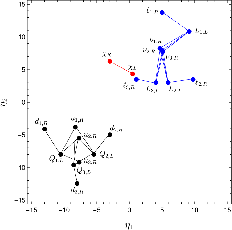
Figure 1: Plot showing locations of fermion wave function centers in the leptophilic version of the model. As defined in the text, the numerical subscript on each fermion field is the generation index. Toroidal compactification is used, so that $\eta_{\lambda}$ is equivalent to $\eta_{\lambda}\pm\mu L=\eta_{L}\pm 30$. In the online figure, the locations of the lepton wave functions are indicated with the following colors: leptons in blue, $\eta_{\chi_{L,R}}$ in red, and quarks in black.

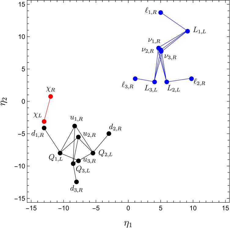
Figure 2: Plot showing locations of fermion wave function centers in the hadrophilic version of the model. The notation is as in the previous figure.

IV.2 Stability of $\chi$

A necessary condition for a dark matter particle is that it must live longer than the age of the universe, $t_{U}$. According to the consensus cosmological model, $t_{U}=13.8\times 10^{9}=4.35\times 10^{17}$ sec pdg_dm . However, this condition is not, general, sufficient; the dark matter must also be sufficiently long-lived to obey constraints from indirect-detection searches. For example, if tree-level and/or loop-level decays yield photons, then constraints from indirect-detection searches, such as those of Fermi-LAT, imply that the lifetime of a dark matter particle $\tau_{DM}$ should obey the lower bound $\tau_{DM}\mathrel{\raisebox{-2.58334pt}{$\stackrel{{\scriptstyle\textstyle>}}{{\sim}}$}}10^{25}$ sec baring . In order to satisfy this constraint in the simplest way, we shall assume that the theory is invariant under a ${\mathbb{Z}}_{2}$ symmetry that operates only on $\chi$ and with respect to which $\chi$ is odd. This guarantees that $\chi$ is stable.

V Calculation of Relic Abundance of Dark Matter

In order to account for the observed relic density of dark matter with a non-self-conjugate DM particle such as the Dirac $\chi$ fermion that we use, it is necessary that the thermal average of the $\chi\bar{\chi}$ annihilation cross section multiplied by (relative) velocity, $v_{r}$, should satisfy the following relation applicable for the time of freeze-out, for the mass range $10\ {\rm GeV}\ \mathrel{\raisebox{-2.58334pt}{$\stackrel{{\scriptstyle\textstyle<}}{{\sim}}$}}m_{\chi}\mathrel{\raisebox{-2.58334pt}{$\stackrel{{\scriptstyle\textstyle<}}{{\sim}}$}}100$ TeV kolb_turner -tulin_yu ,steigman_dm ; steig2

$$\langle\sigma v_{r}\rangle\simeq 4\times 10^{-26}\ \frac{{\rm cm}^{3}}{s}\ .$$ (56)

As will be shown below, this mass range includes the preferred range of values of $m_{\chi}$ in our model. Since our dark matter particle is not non-self-conjugate, there is also the related question of a possible nonzero net number asymmetry $N_{\chi}-N_{\bar{\chi}}$, analogous to the baryon asymmetry in the universe. While asymmetric dark matter models are of interest zurek_adm , we do not assume a $N_{\chi}-N_{\bar{\chi}}$ number asymmetry here.

We will calculate the value of $\langle\sigma v_{r}\rangle$ in our model and set it equal to the value in Eq. (56) to constrain the model. For this purpose, we first determine the dominant contribution to the reaction in which $\chi$ and $\bar{\chi}$ annihilate, yielding SM particles. Given the suppression in the mixing of the U(1)_z gauge field $C_{\mu}$ with the SU(2)_L $A^{3}_{\mu}$ and the U(1)_Y $B_{\mu}$ gauge fields, we may obtain an approximate estimate of the relic abundance by calculating the contribution from a process in which the $\chi$ and $\bar{\chi}$ annihilate to produce a virtual U(1)_z gauge boson $C$ in the $s$ channel, which then materializes into the final-state SM fermion-antifermion pair, $f\bar{f}$. Recall that with the spontaneous breaking of the U(1)_z gauge symmetry, the U(1)_z vector boson, $C$, picks up a mass $m_{C}=g_{z}v_{\omega}/2$ (where, as noted above, the mixing with $A^{3}$ and $B$ is negligibly small, so that $C$ is both an interaction eigenstate and, to a very good approximation, a mass eigenstate). Our solution to fit the relic abundance of the dark matter will entail the inequality $m_{C}\gg m_{\chi}$, so that the the momentum dependence in the U(1)_z vector propagator is negligible. Hence, denoting $s=(p_{\chi}+p_{\bar{\chi}})^{2}$ as the center-of-mass (CM) energy squared in the $\chi\bar{\chi}$ annihilation reaction at relevant times in the early universe, where $p_{\chi}$ and $p_{\bar{\chi}}$ are the four-vectors of the $\chi$ and $\bar{\chi}$, we have

$$\frac{g_{z}^{2}}{m_{C}^{2}-s}\simeq\frac{g_{z}^{2}}{m_{C}^{2}}=\frac{4}{v_{\omega}^{2}}\ .$$ (57)

In the $d=4+n$ space, the resultant amplitude (suppressing the generational index $a$ on the SM fermions $f_{a,L}$ and $f_{a,R}$) is proportional to

$$[\bar{\chi}\gamma_{\mu}\chi][\bar{f}\gamma^{\mu}f] = \Big{(}[\bar{\chi}_{L}\gamma_{\mu}\chi_{L}]+([\bar{\chi}_{R}\gamma_{\mu}\chi_{R}]\Big{)}\,\times$$ (58)

$$\times \Big{(}[\bar{f}_{L}\gamma_{\mu}f_{L}]+[\bar{f}_{R}\gamma_{\mu}f_{R}]\Big{)}\ .$$ (60)

Together with the $\gamma$ matrix structure and Dirac spinors, these operator products involve a sum of products of $y$-dependent wave functions, namely

$$A_{f}^{2}\Big{[}e^{-2(\|\eta-\eta_{\chi_{L}}\|^{2}+\|\eta-\eta_{f_{L}}\|^{2})}+e^{-2(\|\eta-\eta_{\chi_{L}}\|^{2}+\|\eta-\eta_{f_{R}}\|^{2})}+e^{-2(\|\eta-\eta_{\chi_{R}}\|^{2}+\|\eta-\eta_{f_{L}}\|^{2})}+e^{-2(\|\eta-\eta_{\chi_{R}}\|^{2}+\|\eta-\eta_{f_{R}}\|^{2})}\Big{]}\ .$$ (61)

Upon integration over the $y$ coordinates, the first of these yields a term proportional to $e^{-\|\eta_{\chi_{L}}-\eta_{f_{L}}\|^{2}}$, and so forth for the others (see the general integration formula (A2) in bvd ). It follows that the dominant contribution to the low-energy effective Lagrangian from these four-fermion operators in $d=6$ dimensions arises from the term with the smallest distance between (chiral components of) $\chi$ and $f$. For the case where this smallest-distance criterion picks out the four-fermion product $[\bar{\chi}_{k}\gamma_{\mu}\chi_{k}][\bar{f}_{a,k^{\prime}}\gamma^{\mu}f_{a,k^{\prime}}]$ with generational index $a$ for the SM fermion $f_{a,k^{\prime}}$ gennote and chiralities $(k,k^{\prime})$ taking value(s) in the set $\{(L,L),\ (L,R),\ (R,L),\ (R,R)\ \}$, the dominant term is then proportional to

$$[\bar{\chi}_{k}\gamma_{\mu}\chi_{k}][\bar{f}_{a,k^{\prime}}\gamma^{\mu}f_{a,k^{\prime}}]\ .$$ (62)

Carrying out the integration over the wave functions in the extra dimensions, as in nnb02 ; bvd ; nuled , we obtain the following term in the low-energy 4D effective Lagrangian:

$${\cal L}^{(\chi_{k}f_{a,k^{\prime}})}_{\rm eff,\ int.}=\frac{c^{(\chi_{k}f_{a,k^{\prime}})}}{\Lambda_{\rm eff}^{2}}[\bar{\chi}_{k}\gamma_{\mu}\chi_{k}][\bar{f}_{a,k^{\prime}}\gamma^{\mu}f_{a,k^{\prime}}]+h.c.$$ (63)

where

$$c^{(\chi_{k}f_{a,k^{\prime}})}=\frac{\xi^{2}}{\pi}\,e^{-\|\eta_{\chi_{k}}-\eta_{f_{a,k^{\prime}}}\|^{2}}$$ (64)

and

$$\frac{1}{\Lambda_{\rm eff}^{2}}=\frac{g_{z}^{2}z_{\chi}z_{f_{k^{\prime}}}}{m_{C}^{2}}=\frac{4z_{\chi}z_{f_{k^{\prime}}}}{v_{\omega}^{2}}\ .$$ (65)

V.1 Leptophilic Dark Matter

We proceed to calculate the relic abundance of the dark matter in the various versions of the model, beginning with the leptophilic version. With our illustrative placement of the $\chi_{L}$ and $\chi_{R}$ wave function centers shown in Fig. 1, the minimal-distance wave function pair links $\chi_{k}=\chi_{L}$ with $f_{a,k^{\prime}}=\ell_{3,R}\equiv\tau_{R}$. The resultant cross section is

$$\sigma=\frac{s}{48\pi\Lambda_{\rm eff}^{4}}\,|c^{(\chi_{L}\tau_{R})}|^{2}\,\bigg{[}\frac{1-\frac{4m_{\tau}^{2}}{s}}{1-\frac{4m_{\chi}^{2}}{s}}\bigg{]}^{1/2}\,\bigg{[}1-\frac{(m_{\chi}^{2}+m_{\tau}^{2})}{s}+\frac{4m_{\chi}^{2}m_{\tau}^{2}}{s^{2}}\bigg{]}\ ,$$ (66)

where

$$c^{(\chi_{L}\tau_{R})}=\frac{\xi^{2}}{\pi}e^{-\|\eta_{\chi_{L}}-\eta_{\tau_{R}}\|^{2}}\ .$$ (67)

In the center-of-mass frame, the magnitudes of the velocities of the colliding $\chi$ and $\bar{\chi}$ are given by $v_{\chi,CM}=v_{\bar{\chi},CM}=\sqrt{1-(4m_{\chi}^{2}/s)}$, and their relative velocity is $v_{r}=2v_{\chi,CM}$. The quantity that enters into the determination of the relic density is $\langle\sigma v_{r}\rangle$ in general and, in particular, at the time of freeze-out. Since this freeze-out occurs when the temperature satisfies $k_{B}T_{f.o.}/m_{\chi}\simeq 0.05$ swo ; gondolo_gelmini , it follows that the $\chi$ fermions are moderately nonrelativistic at this time, and $s\simeq 4m_{\chi}^{2}$. As the temperature decreases to $T_{\rm f.o.}$, just before the dark matter $\chi$ fermions drop out of thermal equilibrium, and using the nonrelativistic equipartition theorem, we have

$$\frac{m_{\chi}v_{\chi,CM}^{2}}{2}=\frac{3}{2}k_{B}T\sim\frac{3}{2}\Big{(}\frac{m_{\chi}}{20}\Big{)}\ ,$$ (68)

so $v_{\chi,CM}^{2}\simeq 0.08\ll 1$ For approximate estimates, this motivates an expansion of $\langle\sigma v_{r}\rangle$ in powers of $v_{\chi,CM}$. Performing this expansion, using the fact that $v_{\chi,CM}^{2}\simeq 0.08\ll 1$, and anticipating the result that $m_{\tau}/m_{\chi}\ll 1$ from our fit to the relic density, we thus obtain the approximate analytic formula

$$\langle\sigma v_{r}\rangle = \frac{|c^{(\chi_{L}\tau_{R})}|^{2}m_{\chi}^{2}}{8\pi\Lambda_{\rm eff}^{4}}\,\Big{[}1+O(v_{\chi,CM}^{2})\Big{]}$$ (69)

$$\simeq \frac{|c^{(\chi_{L}\tau_{R})}|^{2}m_{\chi}^{2}}{8\pi\Lambda_{\rm eff}^{4}}\ .$$ (71)

Setting this expression for $\langle\sigma v_{r}\rangle_{\rm f.o.}$ equal to the value $4\times 10^{-26}$  cm³/s in Eq. (56), inserting Eq. (67) for $c^{(\chi_{L}\tau_{R})}$, and substituting $\xi=30$, we obtain

$$2\ln\Big{(}\frac{\Lambda_{\rm eff}}{100\ {\rm TeV}}\Big{)}-\ln\Big{(}\frac{m_{\chi}}{10\ {\rm TeV}}\Big{)}+\|\eta_{\chi_{L}}-\eta_{\tau_{R}}\|^{2}=-0.02.$$ (72)

This, then, is the condition for the parameters $\Lambda_{\rm eff}$, $m_{\chi}$, and $\|\eta_{\chi_{L}}-\eta_{\tau_{R}}\|^{2}$ in order for our model to produce the observed dark matter relic density. It is easy to choose parameters that satisfy this condition. For example, we may take $\|\eta_{\chi_{L}}-\eta_{\chi_{R}}\|=4$, which gives $m_{\chi}=10$ TeV, and $\|\eta_{\chi_{L}}-\eta_{\tau_{R}}\|=1$, as shown in Fig. 1. Combined with $\Lambda_{\rm eff}=60$ TeV, this satisfies Eq. (72).

To confirm the accuracy of this approximate analytic approach to the calculation of the relic dark matter density, we have carried out a full numerical computation of the relic density and direct detection cross-section using micrOMEGAs micromegas (which computes the matrix elements using CalcHEP calchep with LanHEP inputs lanhep ). As is evident in Figs. 3 and 4, we find excellent agreement between our approximate analytic results and the results of the full numerical calculation. In general, as shown by Eq. (72), Figs. 3, and 4, one can easily choose the parameters $\Lambda_{\rm eff}$, $m_{\chi}$ (and hence $\|\eta_{\chi_{L}}-\eta_{\chi_{R}}\|$ via Eq. (16)), and $\|\eta_{\chi_{L}}-\eta_{\ell_{3,R}}\|$ to obtain the observed relic dark matter density. A word is in order concerning the upper bound on thermal WIMP dark matter particles from unitarity gkbound -smirnov_beacom . After refinements, the current value of this upper bound is $m_{\chi}<100$ TeV for non-self-conjugate dark matter smirnov_beacom , and this is the reason that we have shown fits with $m_{\chi}$ bounded above by this limit. The range of $m_{\chi}$ values for which we find satisfactory fits to the relic abundance of dark matter is thus consistent with the unitarity upper bound.

It should be emphasized that there is considerable freedom in the model concerning the placement of the wave function centers for $\chi_{L}$ and $\chi_{R}$ relative to the SM leptons in the extra dimensions. For example, we could have chosen the $\chi$ wave function centers to have $\chi_{L}$ and $\chi_{R}$ reversed, so that it is $\chi_{R}$ that is closer to the wave function center for $\ell_{3,R}$. In this case, the dominant four-fermion operator relevant for $\chi\bar{\chi}$ annihilation to SM fermions would have been given by Eq. (62) with $f_{a,k^{\prime}}=\ell_{3,R}$ but with $k=R$ instead of $k=L$. However, this would lead to the same expression (66) for $\langle\sigma v_{r}\rangle$. Moreover, rather than placing the wave function center for $\chi_{L}$ or $\chi_{R}$ closer to $\ell_{3,R}$, we could, instead, have placed it closer to a different lepton such as $\ell_{2,R}$ (staying within the leptophilic version of the model). This would not change our general conclusions concerning the ability of the model to successfully account for the relic density of dark matter.

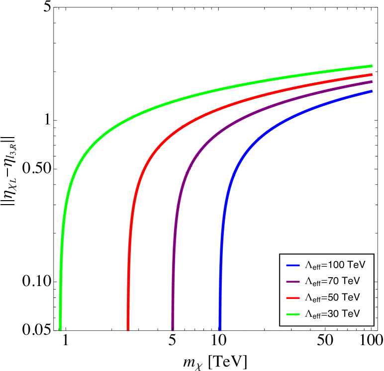
Figure 3: Values of $m_{\chi}$ and $d_{\chi\tau}=\|\eta_{\chi_{L}}-\eta_{\tau_{R}}\|$ that yield the observed dark matter relic density in the leptophilic version of the model, as given by the approximate analytic solution in eq. (72). Curves are plotted for several values of $\Lambda_{\rm eff}$.

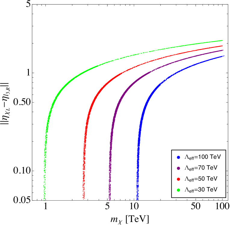
Figure 4: Values of $m_{\chi}$ and $d_{\chi\tau}=\|\eta_{\chi_{L}}-\eta_{\tau_{R}}\|$ that yield the observed dark matter relic density in the leptophilic version of the model, as calculated numerically using micrOMEGAs. Curves are plotted for several values of $\Lambda_{\rm eff}$.

V.2 Hadrophilic Dark Matter

As indicated in Fig. 2, one can also choose the $\chi_{L}$ and $\chi_{R}$ wave function centers to lie closer to the quarks. Hence, in this case the exponential suppression effect in the low-energy, long-distance effective field theory resulting from the large separation of the dark matter from the lepton wave function centers in the extra dimensions means that the dominant interaction of the dark matter is with quarks. This version of the model may thus be called hadrophilic (and also leptophobic).

Direct detection searches xenon1T ; LUX ; PandaX ; PICO have yielded stringent upper limits on the spin-independent and spin-dependent cross sections of the dark matter scattering with nucleons. As the nucleons interacting with the dark matter are primarily composed of first-generation quarks, $u$ and $d$, these direct-detection upper bounds are relevant only if the $\chi_{L}$ and/or $\chi_{R}$ wave function centers are located near to a first-generation quark. As in the case of leptophilic dark matter, one can achieve the observed relic abundance while simultaneously satisfying the direct-detection bounds by localizing the dark matter near to higher-generation quarks in the extra dimensions. Hence, the only nontrivial case to consider is the case in which the dark matterr is localized in the extra dimensions near to a first-generation quark, taken here to be $d_{1,R}$ for illustrative purposes. Furthermore, for definiteness, let us assume that $\chi_{L}$ is located closer to $d_{1,R}$. The same analysis would apply if $\chi_{R}$ were closer to $d_{1,R}$. The constraints on the parameters of the model would be similar for the cases when the dark matter is not localized near a first-generation quark, the only difference being that the bounds from direct-detection searches would not yield significant constraints.

Let us proceed to calculate the condition that yields the observed relic abundance. The cross-section for $\bar{\chi}\chi\to\bar{d}_{1}d_{1}$ is similar to Eq. (66), with the inclusion of an additional color factor of $N_{c}=3$. Therefore, the cross section is

$$\sigma = \frac{s}{16\pi\Lambda_{\rm eff}^{4}}\,|c^{(\chi_{L}d_{1,R})}|^{2}\,\bigg{[}\frac{1-\frac{4m_{d}^{2}}{s}}{1-\frac{4m_{\chi}^{2}}{s}}\bigg{]}^{1/2}\times$$ (73)

$$\times \bigg{[}1-\frac{(m_{\chi}^{2}+m_{d}^{2})}{s}+\frac{4m_{\chi}^{2}m_{d}^{2}}{s^{2}}\bigg{]}\ ,$$ (75)

where

$$c^{(\chi_{L}d_{1,R})}=\frac{\xi^{2}}{\pi}e^{-\|\eta_{\chi_{L}}-\eta_{d_{1,R}}\|^{2}}\ .$$ (76)

(In Eq. (75) we retain the $m_{d}$ terms only for symmetry; they are negligibly small.) From Eq. (65), it is evident that $\Lambda_{\rm eff}$ depends on $z_{d_{1,R}}$. To simplify the notation, we absorb this dependence in the notation and define $\Lambda_{\rm eff}^{(\chi_{L}d_{1,R})}\equiv\Lambda_{\rm eff}$. As before, we expand $\langle\sigma v_{r}\rangle$ in powers of $v_{\chi,CM}$, and obtain

$$\langle\sigma v_{r}\rangle = \frac{3m_{\chi}^{2}}{8\pi\Lambda_{\rm eff}^{4}}|c^{(\chi_{L}d_{1,R})}|^{2}\bigg{[}1+\mathcal{O}(v_{\chi,CM}^{2})\bigg{]}$$ (77)

$$\simeq \frac{3m_{\chi}^{2}}{8\pi\Lambda_{\rm eff}^{4}}|c^{(\chi_{L}d_{1,R})}|^{2}$$ (79)

$$= \frac{3m_{\chi}^{2}}{8\pi\Lambda_{\rm eff}^{4}}\,\bigg{(}\frac{\xi^{2}}{\pi}\bigg{)}^{2}\,e^{-2\|\eta_{\chi_{L}}-\eta_{d_{1,R}}\|^{2}}\ .$$ (81)

Equating this with $\langle\sigma v_{r}\rangle\simeq 4\times 10^{-26}{\rm cm}^{3}/{\rm s}$ and substituting $\xi=30$, we obtain

$$2\ln\Big{(}\frac{\Lambda_{\rm eff}}{100\ {\rm TeV}}\Big{)}-\ln\Big{(}\frac{m_{\chi}}{10\ {\rm TeV}}\Big{)}+\|\eta_{\chi_{L}}-\eta_{d_{1,R}}\|^{2}=0.53\ .$$ (82)

For example, we can choose $\|\eta_{\chi_{L}}-\eta_{d_{1,R}}\|=1$, $\Lambda_{\rm eff}=79$ TeV, and $\|\eta_{\chi_{L}}-\eta_{\chi_{R}}\|=4$ as shown in Fig. 2, which yields $m_{\chi}=10$ TeV. This illustrative choice satisfies Eq. (82).

We use the nucleonAmplitudes routine in the micrOMEGAs micromegas to numerically evaluate the DM-nucleon elastic scattering amplitude. We then use this to calculate the spin-independent and spin-dependent cross-sections of the DM-nucleon scattering for the parameter values satisfying the relic density constraint. We employ the Xenon1T upper bounds xenon1T on the DM-nucleon scattering cross section to constrain our model. For our case, the spin-dependent cross sections are well below the current limits xenon1T , whereas the spin-independent constraints provide non-trivial bounds on the parameters of the hadrophilic version of the model.

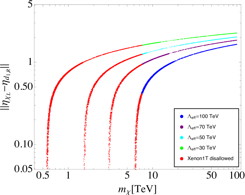
Figure 5: Plot of values of $m_{\chi}$ and $d_{\chi d}=\|\eta_{\chi_{L}}-\chi_{d_{1,R}}\|$ yielding dark matter relic density in agreement with observation in the hadrophilic version of the model, as functions of $\Lambda_{\rm eff}$. The red points produce direct-detection cross sections that are excluded from the Xenon1T bound xenon1T , while the other points represent parameter values that are allowed by both the observed dark matter relic density and the direct-detection bound.

We show these constraints in Fig. 5. The red points yield spin-independent DM-nucleon cross-section values that are excluded from the Xenon1T bound xenon1T . The other colored points are allowed by both the relic abundance constraint and direct-detection bounds. The agreement of the numerical results, as shown in Fig. 5 for the contours yielding the observed relic density, with the approximate analytical formula in Eq. (82) is excellent. A general feature is that as $\Lambda_{\rm eff}$ decreases, the DM-nucleon scattering cross section increases, and this, in turn, requires a larger DM-quark separation in the extra dimensions in order to be consistent with the experimental bounds. Analogous bounds from LUX LUX and PandaX-II PandaX are somewhat less stringent in the $\chi$ mass range relevant here. Our general conclusion for the hadrophilic version of our model is thus similar to the conclusion that we reached for the leptophilic version, namely that there is a substantial range of choices for the parameters $\Lambda_{\rm eff}$, $m_{\chi}$, and $\|\eta_{\chi_{L}}-\eta_{d_{1,R}}\|$ such that the model yields a value for the dark matter relic density that matches observation and is also in accord with bounds from direct-detection searches for dark matter.

VI Experimental and Observational Tests

In this section we discuss experimental tests of the model. One can distinguish two types of tests: (i) searches for evidence of extra spatial dimentions per se, independent of issues of dark matter, and (ii) searches for particle dark matter of the type considered here.

Concerning tests of type (i), we again note that the type of extra-dimensional model used here as ; ms is quite different from the type in which there is a low scale of quantum gravity dif ; ged , as is clear from the fact that the compactification scale here is $L=2\times 10^{-19}$ cm, much smaller than the typical micron-size compactification scale in models considered in ged . As discussed in nuled ; kk , bounds on flavor-changing neutral current effects and precision electroweak data provide significant constraints on this type of extra-dimensional model. Owing to the high energy scale $\Lambda_{L}=100$ TeV corresponding to the inverse compactification scale, experiments at the Tevatron and Large Hadron Collider do not yield constraints on the extra-dimensional aspects of the model.

With regard to searches for dark matter via direct detection, the two leptophilic and hadrophilic versions of the model have quite different properties. As noted above, the leptophilic version of the model easily satisfies bounds from direct detection searches. In contrast, in the hadrophilic version of the model, if one places the wave function center of $\chi_{L}$ and/or $\chi_{R}$ near to a first-generation quark in the extra dimensions, then the bounds from direct detection dark matter searches are non-trivial, as shown in Fig. 5. Future direct-detection searches will improve the bounds on spin-independent and spin-dependent DM-nucleon cross-sections, which will further constrain the parameters shown in Fig. 5.

With regard to indirect detection, since we have constructed the model so that the $\chi$ dark matter fermion is stable, we only discuss constraints due to $\chi\bar{\chi}$ annihilation. This annihilation yields SM particles in the final states, and these have been searched for by several ground-based and space-based instruments. The current bounds on the thermal-average cross-section from indirect-detection experiments such as Fermi-LAT and MAGIC exclude thermally produced DM particle masses of up to 10-100 GeV fermiLAT ; fermiLAT_MAGIC . As is evident from our results in Figs. 4 and 5, the range of masses $m_{\chi}$ for which we fit the observed cosmological dark matter relic density is consistent with these bounds from indirect-detection experiments. Future indirect-detection searches plan to achieve sensitivity to thermal dark matter cross-sections in the multi-TeV range and should improve bounds to constrain the parameter spaces of the thermally produced DM models that we have presented.

As regards collider searches for dark matter particles, because $m_{\chi}$ is typically in the multi-TeV range and interacts very weakly with SM particles, these searches do not probe our model very stringently. Clearly, collider searches at higher-energies would improve the reach of these probes.

It is also of interest to investigate the strength of the self-interactions of the DM $\chi$ fermions. One motivation for this is that there have been arguments that, although collisionless cold dark matter, as embodied in the standard $\Lambda$CDM paradigm (with $\Lambda$ referring to dark energy), fits cosmological data on large-distance scales of order 100 Mpc to Gpc nfw ; binney_tremaine , it may encounter problems on shorter-distance scales of order 1-20 kpc. These problems include (i) the core-cusp problem, i.e., the CDM prediction of too high mass densities at centers of galaxies; (ii) the CDM prediction of substantially more dwarf satellite galaxies than are observed (although, the number of observed dwarf galaxies associated with the Milky Way has been substantially increased by recent observations); and (iii) the so-called “too-big-to-fail” problem of star formation in satellite galaxies moore -boylan_kolchin . These have led to the consideration of models in which the dark matter has substantial self-interactions bullock_boylan_kolchin ; tulin_yu , spergel_steinhardt - kaplinghat2020 . Inclusion of baryon feedback effects in dark matter simulations may alleviate or remove these problems springel -peter . (Other approaches to dark matter that address these issues have also been studied, e.g., wdm -fdm .) Further observational work and improvement of theoretical modelling of structure formation should elucidate how serious the possible problems are for the $\Lambda$CDM paradigm. However, at least this motivates an assessment of the size of the $\chi$ self-interactions here.

The self-interactions of the dark matter particle in our model involve $\chi\bar{\chi}\to\chi\bar{\chi}$ reactions and $\chi\chi\to\chi\chi$ (and $\bar{\chi}\bar{\chi}\to\bar{\chi}\bar{\chi}$) reactions, which are the DM analogues of Bhabha and Møller scattering in quantum electrodynamics. The $\chi\bar{\chi}\to\chi\bar{\chi}$ involves exchange of the U(1)_z vector boson $C$ in the $s$ channel and $t$ channel, while the $\chi\chi\to\chi\chi$ reaction involves only the $C$ exchange in the $t$ channel. For our purposes, a rough estimate of these cross sections will be sufficient. Since $m_{C}\gg m_{\chi}$, the propagator is well approximated by a constant. Thus, the amplitudes for the reactions have a prefactor $z_{\chi}^{2}g_{z}^{2}/m_{C}^{2}=4z_{\chi}^{2}/v_{\omega}^{2}$. The operator product in the $d=6$ dimensional space is the analogue of Eq. (60) with $f=\chi$, and involves the products of Gaussian factors listed in Eq. (61) with this substitution $f=\chi$. Of the four products of Gaussians, the dominant ones are those in which the $\chi$ and $\bar{\chi}$ wave function centers are at the same point in the extra dimensions, namely $A_{f}^{2}e^{-4\|\eta-\eta_{\chi_{L}}\|^{2}}$ and $A_{f}^{2}e^{-4\|\eta-\eta_{\chi_{R}}\|^{2}}$. After integration of these operator products over the extra dimensions, we obtain the resultant low-energy 4D effective operators for the $\chi$ self-interaction (SI):

$${\cal L}_{\rm SI,4D,eff}\simeq\Big{(}\frac{4z_{\chi}^{2}}{v_{\omega}^{2}}\Big{)}\,\Big{(}\frac{\xi^{2}}{\pi}\Big{)}\times$$ (83)

$$\times \bigg{[}[\bar{\chi}_{L}\gamma_{\mu}\chi_{L}][\bar{\chi}_{L}\gamma^{\mu}\chi_{L}]+[\bar{\chi}_{R}\gamma_{\mu}\chi_{R}][\bar{\chi}_{R}\gamma^{\mu}\chi_{R}]\bigg{]}\ .$$ (85)

The resultant cross sections for the $\chi\bar{\chi}\to\chi\bar{\chi}$ and $\chi\chi\to\chi\chi$ reactions at a center-of-mass energy $s\mathrel{\raisebox{-2.58334pt}{$\stackrel{{\scriptstyle\textstyle>}}{{\sim}}$}}4m_{\chi}^{2}$ are

$$\sigma_{SI}\sim\Big{(}\frac{4z_{\chi}^{2}}{v_{\omega}^{2}}\Big{)}^{2}\,\Big{(}\frac{\xi^{2}}{\pi}\Big{)}^{2}\,m_{\chi}^{2}R_{2}\ ,$$ (88)

where $R_{2}$ denotes the two-body final-state phase space, $R_{2}<1/(8\pi)$. Using the illustrative values $g_{z}\sim 0.5$, $z_{\chi}\sim 1$, $v_{\omega}\simeq 400$ TeV together with a value $m_{\chi}=10$ TeV in accord with our fit to the DM relic density, and again using the $\xi=30$ characterizing our basic extra-dimensional framework, we find that these cross sections are $\sim 10^{-35}$ cm² and hence $\sigma_{SI}/m_{\chi}\sim 10^{-39}\ {\rm cm}^{2}/{\rm GeV}\sim 10^{-15}\ {\rm cm}^{2}/{\rm g}$ (where the conversion $1\ {\rm cm}^{2}/{\rm g}=1.8\times 10^{-24}\ {\rm cm}^{2}/{\rm GeV}$ is used). Although these are just rough estimates, they show that the self-interactions of the $\chi$ fermions are much smaller than the general range $0.1\mathrel{\raisebox{-2.58334pt}{$\stackrel{{\scriptstyle\textstyle<}}{{\sim}}$}}\sigma_{SI}/m_{DM}\mathrel{\raisebox{-2.58334pt}{$\stackrel{{\scriptstyle\textstyle<}}{{\sim}}$}}1$ cm²/g that is determined by fits to cosmological observations (e.g., tulin_yu ) in the framework of a self-interacting dark matter particle with mass $m_{DM}$. Hence, our dark matter particle is a WIMP with very small self-interactions.

VII Conclusions

In this work we have constructed and studied a model for dark matter with $n=2$ extra spatial dimensions in which Standard-Model fermions have localized wave functions. The underlying gauge group is $G_{\rm SM}\otimes{\rm U}(1)_{z}$ and the dark matter particle is a SM-singlet Dirac fermion, $\chi$, charged under the ${\rm U}(1)_{z}$ gauge symmetry. The communication between the dark matter sector and the SM fields arises mainly from the property that the SM fermions are charged under the U(1)_z gauge interaction. This communication is naturally weak, so $\chi$ is a weakly interacting massive particle, which, furthermore, has negligibly small self-interactions. We have focused on a subclass denoted $C_{1}$ in which a seesaw mechanism is operative that naturally explains small masses for the observed neutrinos. Within this subclass we have studied two versions of the model, namely leptophilic and hadrophilic and have demonstrated that each of these can account for cosmological observations on the relic dark matter density. These fits allow a range of dark matter masses, typically in the multi-TeV range. Constraints from direct-detection searches for dark matter can be relevant for the hadrophilic version of the model, and we have determined the values of the parameters that satisfy these constraints. We also discuss experimental tests of the model.

Separately from our application to dark matter, we have shown how the model constitutes a counterexample to conventional wisdom in effective field theory claiming that a Dirac fermion naturally has a mass lying at the ultraviolet cutoff. The reason that this conventional lore does not apply here is due to the exponentially strong suppression of the 4D Dirac fermion mass arising from the separate location of the $\chi_{L}$ and $\chi_{R}$ wave function centers in the extra dimensions. As a consequence of this suppression, for a moderate dimensionless distance $\|\eta_{\chi_{L}}-\eta_{\chi_{R}}\|$ in the extra dimensions, the $\chi$ mass parameter in the higher-dimensional space can be at the UV cutoff while the physically observed $m_{\chi}$ is much smaller than this UV cutoff.

Appendix A Neutral Vector Boson Masses and Mixing

In this appendix we briefly remark on neutral vector boson masses and mixing in this model. This will be treated in the context of the low-energy 4D effective field theory. A covariant derivative acting on the SM Higgs field $H$ is

$$D_{\mu}H=\Big{(}{\mathbb{I}}_{2\times 2}\partial_{\mu}-ig{\vec{T}}\cdot{\vec{A}}_{\mu}-\frac{g^{\prime}Y_{H}}{2}B_{\mu}-\frac{g_{z}z_{H}}{2}C_{\mu}\Big{)}\,H\ ,$$ (89)

where ${\vec{A}}_{\mu}$, $B_{\mu}$, and $C_{\mu}$ are the gauge fields for the SU(2)_L, U(1)_Y, and U(1)_z gauge interactions; $g$, $g^{\prime}$, and $g_{z}$ are the respective gauge couplings, $Y_{H}=1$ is the weak hypercharge of the SM Higgs $H$, and $z_{H}$ is the U(1)_z charge of the $H$. A covariant derivative acting on the additional Higgs field $\omega$ is

$$D_{\mu}\omega=\Big{(}\partial_{\mu}-i\frac{g_{z}}{2}C_{\mu}\Big{)}\,\omega\ ,$$ (90)

with the vacuum expectation values

$$\langle H\rangle_{0}=\left(\begin{array}[]{c}0\\ \frac{v}{\sqrt{2}}\end{array}\right)\ .$$ (91)

and

$$\langle\omega\rangle_{0}=\frac{v_{\omega}}{\sqrt{2}}\ ,$$ (92)

these yield the following mass-squared terms for the neutral gauge fields in the 4D Lagrangian:

$$\frac{v^{2}}{8}(-gA^{3}_{\mu}+g^{\prime}B_{\mu}+g_{z}z_{H}C_{\mu})(-gA^{3\mu}+g^{\prime}B^{\mu}+g_{z}z_{H}C^{\mu})$$ (93)

(94)

$$+\frac{g_{z}^{2}v_{\omega}^{2}}{8}C_{\mu}C^{\mu}\ .$$ (95)

The resultant mixing has been analyzed in adh and has the property that in the limit $g_{z}v_{\omega}\gg z_{H}v$, the mixing between $C_{\mu}$ and the SM gauge fields $A^{3}_{\mu}$ and $B_{\mu}$ vanishes. Specifically, in this limit, the mixing angle vanishes like $z_{H}(g^{2}+g^{\prime 2})^{1/2}v/(g_{z}v_{\omega})$. Since we assume the above inequality $g_{z}v_{\omega}\gg z_{H}v$, we neglect this mixing here. (Recall that the SM factor $(g^{2}+g^{\prime 2})^{1/2}\simeq 0.74$ at a reference scale $m_{Z}$, where $g$ and $g^{\prime}$ are the running SU(2)_L and U(1)_Y gauge couplings; for a general discussion of effects of heavy neutral vector bosons, see, e.g., pgl .) We also make use of the fact, as discussed in adh ; holdom , that at a given scale one can perform a rotation in the $(B_{\mu},C_{\mu})$ space to eliminate a kinetic mixing term $\propto B_{\mu\nu}C^{\mu\nu}$ in the effective action, so that it is only generated at loop level.

References

- (1) See, e.g., Particle Data Group, Review of Particle Properties online at http://pdg.lbl.gov and L. Baudis and S. Profumo, Dark Matter Minireview at this website.
- (2) Specifically, defining , where , with the current Hubble constant, the Newton gravitational constant, and the mass density of a constituent , current cosmological observations yield the results for the matter density, for the dark matter density, and for the baryon matter density pdg_dm .
- (3) E. Kolb and M. Turner, The Early Universe (Westview Press (1994)).
- (4) G. Jungman, M. Kamionkowski, and K. Griest, Phys. Rept. 267, 195 (1996).
- (5) G. Bertone, D. Hooper, and J. Silk, Phys. Rept. 405, 279 (2005).
- (6) L. E. Strigari, Phys. Rept. 531, 1 (2013).
- (7) M. Battaglieri et al., arXiv:1707.04591.
- (8) J. S. Bullock and M. Boylan-Kolchin, Ann. Rev. Astron. Astrophys. 55, 343 (2017).
- (9) S. Tulin and H.-B. Yu, Phys. Rept. 730, 1 (2018).
- (10) G. Arcadi, M. Dutra, P. Ghosh, M. Lindner, and Y. Mambrini, Eur. Phys. J. C 78, 203 (2018).
- (11) C. Blanco, M. Escudero, D. Hooper, and S. J. Witte, JCAP 11 (2019) 024.
- (12) For a recent discussion of contributions to dark matter from primordial black holes, see B. Carr and F. Kühnel, Ann. Rev. Nucl. Part. Sci. 70, 355 (2020).
- (13) Inserting the generational index we have, for example, , , ; , , ; , , , etc.
- (14) N. Arkani-Hamed and M. Schmaltz, Phys. Rev. D 61, 033005 (2000).
- (15) E. A. Mirabelli and M. Schmaltz, Phys. Rev. D 61, 113011 (2000).
- (16) S. Nussinov and R. Shrock, Phys. Rev. Lett. 88, 171601 (2002).
- (17) S. Girmohanta and R. Shrock, Phys. Rev. D 101, 015017 (2020).
- (18) S. Girmohanta and R. Shrock, Phys. Rev. D 101, 095012 (2020)
- (19) S. Girmohanta, Eur. Phys. J. C 81, 143 (2021).
- (20) S. Girmohanta, R. N. Mohapatra, and R. Shrock, Phys. Rev. D 103, 015021 (2021).
- (21) See, e.g., W.-F. Chung, I-L. Ho, and J. N. Ng, Phys. Rev. D 66, 076004 (2002); W.-F. Chung and J. N. Ng, Phys. Rev. D 68, 116002 (2003); Y. Grossman and G. Perez, Phys. Rev. D 67, 015011 (2003); B. Lille and J. Hewett, Phys. Rev. D 68, 116002 (2003).
- (22) Note that this model is quite different from models in which only gravitons propagate in the extra dimensions ged , as is evident from the fact that the compactification scales are quite different. For example, for and a quantum-gravity scale of 30 TeV, the compactification size in the models of Ref. ged is cm, much larger than the scale cm in our model.
- (23) N. Arkani-Hamed, S. Dimopoulos, and G. R. Dvali, Phys. Lett. B 429, 263 (1998); I. Antoniadis, N. Arkani-Hamed, S. Dimopoulos, and G. R. Dvali, Phys. Lett. B 436, 257 (1998); K. R. Dienes, E. Dudas, and T. Gherghetta, Phys.Lett. B 436, 55 (1998); S. Nussinov and R. Shrock, Phys. Rev. D 59, 105002 (1999). See also T. Appelquist, H.-C. Cheng, and B. A. Dobrescu, Phys. Rev. D 64, 035002 (2001); .
- (24) R. N. Mohapatra and J. C. Pati, Phys. Rev. D 11, 2558 (1975); R. N. Mohapatra and R. E. Marshak, Phys. Rev. Lett. 44, 1316 (1980); R. N. Mohapatra and G. Senjanović, Phys. Rev. Lett. 44, 912 (1980).
- (25) S. L. Glashow, J. Iliopoulos, and L. Maiani, Phys. Rev. D 2, 1285 (1970).
- (26) M. K. Gaillard and B. W. Lee, Phys. Rev. D 10, 897 (1974); M. K. Gaillard and B. W. Lee, and R. E. Shrock, Phys. Rev. D 13, 2674 (1976);
- (27) B. W. Lee and R. E. Shrock, Phys. Rev. D 16, 1444 (1977).
- (28) T. Appelquist, B. Dobrescu, and A. R. Hopper, Phys. Rev. D 68, 035012 (2003).
- (29) L. J. Hall, K. Jedamzik, J. March-Russell and S. M. West, JHEP 03 (2010) 080.
- (30) F. Elahi, C. Kolda, and J. Unwin, JHEP 03 (2015) 048.
- (31) N. Bernal, M. Heikinheimo, T. Tenkanen, K. Tuominen and V. Vaskonen, Int. J. Mod. Phys. A 32, 1730023 (2017).
- (32) M. G. Baring, T. Ghosh, F. S. Queriroz, and K. Sinha, Phys. Rev. D 93, 103009 (2016).
- (33) G. Steigman, Phys. Rev. D 91, 083538 (2015) and references therein,.
- (34) Parenthetically, it may be recalled that if the dark matter were a self-conjugate particle, then the right-hand side of Eq. (56) would be reduced by half, to cm3/s steigman_dm .)
- (35) See, e.g., K. Zurek, Phys. Rept. 537, 91 (2014).
- (36) M. Srednicki, R. Watkins, and K. A. Olive, Nucl. Phys. B 310, 693 (1988).
- (37) P. Gondolo and G. Gelmini, Nuc. Phys. B 360, 145 (1991).
- (38) G. Bélanger, F.Boudjema, A.Pukhov, and A.Semenov, Comput. Phys. Commun. 180, 747 (2009); Comput. Phys. Commun. 185, 960 (2014).
- (39) A. Belyaev, N. D. Christensen, and A. Pukhov, Comput. Phys. Commun. 184, 1729 (2013).
- (40) A. Semenov, Comput. Phys. Commun. 201, 167 (2016).
- (41) K. Griest and M. Kamionkowski, Phys. Rev. Lett. 64, 615 (1990).
- (42) S. El Hedri, W. Shepherd, and D. G. E. Walker, Phys. Dark Univ. 18, 127 (2017).
- (43) F. Kahlhoefer, K. Schmidt-Hoberg, T. Schwetz, and S. Vogl, JHEP 02 (2016) 016 (2016).
- (44) J. Smirnov and J. F. Beacom, Phys. Rev. D 100, 043029 (2019).
- (45) E. Aprile et al. (XENON Collaboration), Phys. Rev. Lett. 121, 111302 (2018); Phys. Rev. Lett. 122, 141301 (2019).
- (46) D. S. Akerib et al. (LUX Collaboration) Phys. Rev. Lett. 118, 021303 (2017); Phys. Rev. Lett. 118, 251302 (2017).
- (47) X. Cui et al. (PandaX-II Collaboration), Phys. Rev. Lett. 118, 021303 (2017); J. Xia et al. (PandaX-II Collaboration), Phys. Lett. B 792, 193 (2019).
- (48) C. Amole et al. (PICO Collaboration), Phys. Rev. D 100, 022001 (2019).
- (49) M. Ackermann et al. (FermiLAT Collaboration), Phys. Rev. Lett. 115, 231301 (2015); Phys. Rev. D 89, 042001 (2014).
- (50) M. L. Ahnen et al. (MAGIC and Fermi-LAT Collaborations) JCAP 02 (2016) 039.
- (51) J. F. Navarro, C. S. Frenk, and S. D. M. White, Ap. J. 462, 563 (1996); Ap. J. 490, 493 (1997).
- (52) J. Binney and S. Tremaine, Galactic Dynamics, 2nd ed. (Princeton Univ. Press, Princeton, NJ, 2008).
- (53) B. Moore, S. Ghigna, F. Governato, G. Lake, T. Quinn, J. Stadel, and P. Tozzi, Ap. J. 524, L19 (1999).
- (54) D. N. Spergel and P. J. Steinhardt, Phys. Rev. Lett. 84, 3760 (2000).
- (55) M. Boylan-Kolchin, J. S. Bullock, and M. Kaplinghat, Mon. Not. Roy. Astron. Soc. 415, L40 (2011); 422, 1203 (2012); A. Fitts, M. Boylan-Kolchin, B. Bozek, J. S. Bullock, et al., Mon. Not. Roy. Astron. Soc. 490, 962 (2019).
- (56) R. Essig, S. D. McDermott, H.-B. Yu, and Y.-M. Zhong, Phys. Rev. Lett. 123, 121102 (2019); D. Egana-Ugrinovic, R. Essig, D. Gift, and M. LoVerde, JCAP 05 (2021) 013.
- (57) M. A. Buen-Abad, M. Schmaltz, J. Lesgourgues, and T. Brinckmann, JCAP 01 (2018) 008; A. Sokolenko, K. Bondarenko, T. Brinckmann, J. Zavala, M. Vogelsberger, T. Bringmann, and A. Boyarsky, JCAP 12 (2018) 038;
- (58) K. E. Andrade, J. Fuson, S. Gad-Nasr, D. Kong, Q. Minor, M. G. Roberts, and M. Kaplinghat, arXiv:2012.06611.
- (59) V. Springel, Mon. Not. Roy. Astron. Soc. 364, 1105 (2005); V. Springel, S. D. M. White, A. Jenkins, C. S. Frenk, et al., Nature 435, 625 (2005); C. Scannapieco, M. Wadepuhl, O.H. Parry, J. F. Navarro, A. Jenkins, et al., Mon. Not. Roy. Astron. Soc. 423 1726 (2012).
- (60) T. Sawala, C. S. Frenk, A. Fattahi, J. F. Navarro, et al., Mon. Not. Roy. Astron. Soc. 457, 1931 (2016).
- (61) F. C. van den Bosch, G. Ogiya, O. Hahn, and A. Burkert, Mon. Not. Roy. Astron. Soc. 474, 3043 (2018).
- (62) Y. Kim, A. H. G. Peter, and J. R. Hargis, Phys. Rev. Lett. 121, 211302 (2018).
- (63) See, e.g., K. Abazajian, G. M. Fuller, and M. Patel, Phys. Rev. D 64, 023501 (2001); A. Kusenko, Phys. Rept. 481, 1 (2009).
- (64) R. N. Mohapatra, S. Nussinov, and V. L. Teplitz, Phys. Rev. D 66, 063002 2002).
- (65) L. Hui, J. P. Ostriker, S. Tremaine, and E. Witten, Phys. Rev. D 95, 043541 (2017).
- (66) P. G. Langacker, Rev. Mod. Phys. 81, 1199 (2008).
- (67) B. Holdom, Phys. Lett. B 166, 196 (1986).