The role of scatter and satellites in shaping the large-scale clustering of X-ray AGN as a function of host galaxy stellar mass

Abstract

The co-evolution between central supermassive black holes (BH), their host galaxies, and dark matter halos is still a matter of intense debate. Present theoretical models suffer from large uncertainties and degeneracies, for example, between the fraction of accreting sources and their characteristic accretion rate. In recent work we showed that Active Galactic Nuclei (AGN) clustering represents a powerful tool to break degeneracies when analysed in terms of mean BH mass, and that AGN bias at fixed stellar mass is largely independent of most of the input parameters, such as the AGN duty cycle and the mean scaling between BH mass and host galaxy stellar mass. In this paper we take advantage of our improved semi-empirical methodology and recent clustering data derived from large AGN samples at $z\sim 1.2$, demonstrate that the AGN bias as a function of host galaxy stellar mass is a crucial diagnostic of the BH–galaxy connection, and is highly dependent on the scatter around the BH mass–galaxy mass scaling relation and on the relative fraction of satellite and central active BHs. Current data at $z\sim 1.2$ favour relatively high values of AGN in satellites, pointing to a major role of disc instabilities in triggering AGN, unless a high minimum host halo mass is assumed. The data are not decisive on the magnitude/covariance of the BH-galaxy scatter at $z\sim 1.2$ and intermediate host masses $M_{\mathrm{star}}\lesssim 10^{11}\,\mathrm{M}_{\odot}$. However, future surveys like Euclid/LSST will be pivotal in shedding light on the BH–galaxy co-evolution.

1 Introduction

The presence of supermassive black holes at the centers of virtually every massive galaxy is an accepted paradigm. The masses of these central black holes appear to correlate with the properties of their host galaxies (e.g. Ferrarese & Ford, 2005; Kormendy & Ho, 2013; Graham & Scott, 2015; Reines & Volonteri, 2015; Shankar et al., 2019, 2020) with tentative evidence for a link even with their host dark matter haloes (e.g. Ferrarese, 2002; Bandara et al., 2009). The very existence of such correlations, which are observed to hold even at higher redshifts (e.g. Shankar et al., 2009b; Cisternas et al., 2011b; Shen et al., 2015; Suh et al., 2020), point to a degree of co-evolution between the black holes and their hosts. Thus, unveiling the shape, dispersion and evolution of these correlations represents a crucial task in present-day extra-galactic astronomy to acquire a full picture of galaxy formation and evolution.

Despite decades of observational and theoretical work aimed at deciphering the nature of the black hole-galaxy scaling relations, the causal link between the two remains still unsolved. A strong release of energy/momentum from an accreting central supermassive black hole (BH) shining as an Active Galactic Nucleus (AGN) naturally predicts a tight and constant correlation with velocity dispersion (e.g. Silk & Rees, 1998; Granato et al., 2004), which has been recognized as one of the most fundamental property linked to black hole mass (e.g. Bernardi, 2007; Shankar et al., 2019; Marsden et al., 2020). Merger-driven models of black hole growth would instead predict a tighter correlation with the host galaxy stellar mass (e.g. Jahnke & Macciò, 2011; Hirschmann et al., 2010).

Given the large number of input assumptions in traditional ab initio cosmological models, a more phenomenological complementary approach has been introduced in the last decade to constrain the properties of black holes in a cosmological context. The latter method relies on identifying the overall populations of active and inactive black holes at a given redshift on statistical grounds via, e.g. continuity equation techniques (e.g. Marconi et al., 2004; Shankar et al., 2004, 2013; Aversa et al., 2015) and/or semi-empirical mock catalogues tuned to reproduce stellar mass functions, AGN X-ray luminosity functions and/or AGN clustering properties (e.g. Georgakakis et al., 2019; Aird & Coil, 2021; Allevato et al., 2021)

Further constraints on the co-evolution scenario are indeed provided by studying the spatial clustering of AGN, especially X-ray selected (e.g. Coil et al., 2009; Krumpe et al., 2010; Allevato et al., 2011; Krumpe et al., 2012; Mountrichas & Georgakakis, 2012; Mendez et al., 2016; Powell et al., 2018; Viitanen et al., 2019; Allevato et al., 2019; Powell et al., 2020). Clustering provides an independent way of connecting accreting BHs to their large-scale environments via the link with their underlying dark matter halo population. Several clustering studies have argued that AGN environment could play a significant role in triggering the AGN phase, highlighting the importance of host dark matter halos in nuclear activity (e.g. Hickox et al., 2009; Allevato et al., 2011; Fanidakis et al., 2012; Gatti et al., 2016).

However useful, interpretation of X-ray AGN clustering results have suffered from not properly being able to take into account the host galaxy properties. Indeed what is currently debated is to which degree AGN clustering can be understood solely in terms of the underlying host galaxy properties (e.g. color, stellar mass ${M_{\mathrm{star}}}$, star-formation rate), and AGN selection effects (e.g. Hickox et al., 2009; Mendez et al., 2016; Mountrichas et al., 2019; Viitanen et al., 2019; Powell et al., 2020). Thus of special interest is the host galaxy stellar mass ${M_{\mathrm{star}}}$ due to its intimate connection with the underlying dark matter halo (e.g. Moster et al., 2010; Leauthaud et al., 2012; Behroozi et al., 2019).

In terms of the AGN-hosting dark matter halo connection, despite their extreme flexibility, all phenomenological AGN models suffer from serious degeneracies that cannot be easily broken. Shankar et al. (2020) have shown that the large-scale clustering of AGN, e.g. the bias, as a function of BH mass represents a powerful framework to constrain the normalization and slope of the correlation between BH mass and host galaxy stellar mass. Recently, Allevato et al. (2021) have found by using AGN mock catalogs built on observationally derived galaxy - BH scaling relations, AGN duty cycles (i.e.the probability for a galaxy hosting an active black hole), and Eddington ratio distributions, that the AGN large-scale bias is a crucial diagnostic to break degeneracies in the input AGN model. Other groups have, instead, built the correlation between black hole mass and host halo mass by passing the scaling relation with host galaxy stellar mass or velocity dispersion and the AGN duty cycle (e.g. Georgakakis et al., 2019; Aird & Coil, 2021). Besides not allowing for any quantitative assessment of the underlying fundamental black hole-galaxy scaling relations, limiting the efficacy of these models in shedding light on the processes controlling the co-evolution of BHs and their hosts, the latter approach is still not immune to degeneracies between e.g. duty cycles and Eddington ratio distributions.

In particular, Allevato et al. (2021) have shown at $z\sim 0.1$ that the clustering at fixed stellar mass is largely independent of the input duty cycle, Eddington ratio distribution, and the $M_{\mathrm{star}}$-$M_{\mathrm{halo}}$ relation. This implies that the clustering of normal galaxies matches the AGN clustering at a given stellar mass, provided the AGN hosts are a random subsample of the underlying galaxy population of the same stellar mass. However, as we will show in this work, the AGN large-scale bias as a function of stellar mass is mainly set by the scatter - not so much by the shape - of the BH mass - stellar mass relation and by the relative fraction of AGN in central and satellite dark matter halos. The role of the scatter in the BH - host mass relation on the AGN clustering has been investigated in different studies at high $z\sim 4$ (White et al., 2008; Wyithe & Loeb, 2009; Shankar et al., 2010b; Bonoli et al., 2010). In particular, White et al. (2008) have shown that the very high bias measured for SDSS quasars at $z\sim 4$ by Shen et al. (2007) is in favour of a small scatter in the BH – galaxy scaling relation. In fact, the key idea is that any scatter in the input scaling relation increases the contribution from lower mass and less biased halos, thus decreasing the observed AGN large-scale bias.

However, these studies focus on high redshifts, where the population of supermassive BHs that powers the quasars is growing rapidly and inhabits the rarest, most massive halos. Moreover, they do not investigate the effect of the scatter on the AGN clustering in different stellar mass bins, also bypassing additional parameters that might affect the AGN bias normalization.

Instead, in this work we study the concurring effect of the scatter around the BH mass–galaxy mass relation and of the relative fraction of satellite and central active BHs on the AGN large-scale clustering, focusing our attention on the AGN bias as a function of host galaxy stellar mass at intermediate redshift $z\sim 1$. We thus expand on Allevato et al. (2021) by following their methodology to create realistic mock catalogs of galaxies and active BHs and (i) we include on top of a regular Gaussian scatter a positive covariant correlation between the BH and the host galaxy stellar mass at fixed halo mass; (ii) we focus on redshift $\sim$1.2, i.e. close to the peak of the AGN activity (e.g. Shankar et al., 2009a; Madau & Dickinson, 2014); and (iii) we allow the satellite AGN fraction to vary. Recently Farahi et al. (2019) applied a similar covariant method approach in order to reveal an anti-correlation between hot and cold baryonic mass in galaxy clusters. In the context of BH-galaxy co-evolution, it would expected that a degree of correlation exists between the properties of the central BH and the galaxy, especially in any scenario involving an AGN feedback.

The AGN bias as a function of host galaxy stellar mass is thus a crucial diagnostic of the black hole-galaxy connection which, together with the bias as a function of black hole mass (Shankar et al., 2020), can provide tight constraints on the co-evolution of black holes and galaxies. It is the ideal time to set out the methodology behind the modelling of AGN bias as a function of stellar mass based on the large amount of current and future data. Recent multi-wavelength surveys such as XMM-COSMOS, Chandra COSMOS legacy survey, AEGIS have in fact made it possible to study the AGN environment in terms of host galaxy properties. In particular, several AGN clustering studies have specifically considered AGN clustering as a function of the host galaxy stellar mass (e.g. Georgakakis et al., 2014; Mountrichas et al., 2019; Viitanen et al., 2019; Allevato et al., 2019). Moreover, in the next years the synergy among J-PAS, eROSITA, 4MOST, LSST, Euclid, and JWST will allow us to measure the AGN clustering with high statistics, and to derive host galaxy stellar mass estimates of moderate-to-high luminosity AGN up to $z\sim 2$ to measure the large-scale bias as a function of host galaxy properties of millions of objects at different $z$.

The paper is organized as follows. In Section 2 we will detail the methodology for estimating the covariant scatter and the semi-empirical model to build our AGN mock catalogues. In Section 3 we outline the results, while in sections 4 and 5 we present the discussion and conclusions of this work.

2 Methodology

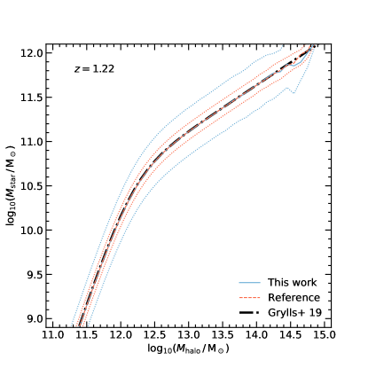
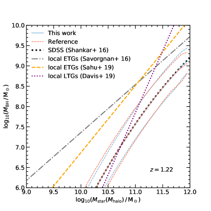
Figure 1: Input scaling relation used to populate DM halos with (active) BHs by assigning host galaxy stellar masses $M_{\mathrm{star}}$ based on given DM halo mass $M_{\mathrm{halo}}$ (left), and BH masses $M_{\mathrm{BH}}$ to given $M_{\mathrm{star}}$ (right). The mean scaling relations are shown as black dash-dotted lines, while two different methods for the scatter in the relations are shown as blue solid (this work, covariant scatter) and red dashed (reference) lines. The width of the distributions ($20\%$ and $80\%$ quantiles) are shown above and below the relations using the same colors and dotted lines.

In this work we will investigate the large-scale clustering properties of X-ray selected AGN, and moreover the imprint of covariant scatter between the central black hole mass ${M_{\mathrm{BH}}}$ and the host galaxy stellar mass ${M_{\mathrm{star}}}$. For this purpose, we create mock catalogs of active and non-active galaxies by using semi-empirical models (SEMs) based on large N-body simulations, and measure the large-scale bias as a function of stellar mass $b({M_{\mathrm{star}}})$ as well as the projected two-point correlation function $w_{\mathrm{p}}(r_{\mathrm{p}})$ of mock AGNs. The full description of numerical routines to create mock catalogs of galaxies and their BHs using SEMs is given in Allevato et al. (2021) at $z\sim 0.1$.

We extend this work to higher redshift $z=1.22$, and investigate the role of covariant scatter in assigning ${M_{\mathrm{star}}}$ and ${M_{\mathrm{BH}}}$ to mock AGNs. We only describe the important steps in the generation of the AGN mock catalogs and we refer the reader to Allevato et al. (2021) for the details.

We note that our results are specific to the redshift of interest, starting from the input DM halo catalog and input scaling relations which evolve with redshift (e.g. Grylls et al., 2019), and upon assigning large-scale bias to DM halos $b=b(M_{\mathrm{halo}},z)$, with bias increasing with $z$ at a given $M_{\mathrm{halo}}$ (Sheth et al., 2001; van den Bosch, 2002).

2.1 Input Scaling Relations

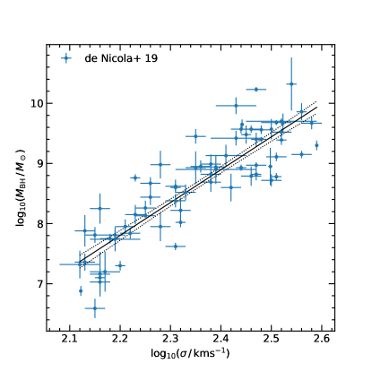
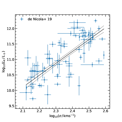
Figure 2: The local galaxy data and the best-fit scaling relations used to derive the covariance matrix of the scatter for ‘This work’. Left and right panels show the velocity dispersion against black hole mass, and K-band luminosity, respectively. The dashed black lines correspond to $16\%$ and $84\%$ quantiles of the best-fit relations based on $20\,000$ Monte Carlo samples.

For building mock catalogs of AGNs, we start from the dark matter (DM) halo catalog extracted from the MultiDark Planck 2 (MDPL2) simulation (Riebe et al., 2013; Klypin et al., 2016) at redshift $z=1.22$, close to the redshift of recent X-ray AGN clustering measurements (e.g. Viitanen et al., 2019; Allevato et al., 2019). The MDPL2 simulation is a cosmological DM only N-body simulation, with a box size of 1 $\,\mathrm{Gpc}/h$, $3\,840^{3}$ DM particles, and a mass resolution of $1.51\times 10^{9}\,\mathrm{M}_{\odot}/h$. The cosmology used in the simulation is flat $\Lambda$CDM with $h=0.6777$, $\sigma_{8}=0.8228$, and $\Omega_{m}=0.307115$. We use the ROCKSTAR (Behroozi et al., 2013) DM halo catalog.The catalogs contain both central/parent halos and satellite halos with unstripped mass at infall, and the 3-dimensional positions for estimating the projected two-point correlation function $w_{\mathrm{p}}$.

In the semi-empirical approach, each halo is assigned a galaxy and central BH (active or not) following the most up-to-date empirical relations. This approach has the benefit of avoiding the need to model physical AGN processes, while reproducing the galaxy/BH statistical properties, such as stellar mass function and luminosity function. First, halos and subhalos are populated with stellar masses ${M_{\mathrm{star}}}$ according to a $M_{\mathrm{star}}=M_{\mathrm{star}}(M_{\mathrm{halo}},z)$ (we drop the explicit $z$ dependence and focus on $z=1.22$ from now on) relation using the Moster et al. (2010) formulae, and the recent updated parameters of Grylls et al. (2019).

Galaxies are then populated with BHs according to an input ${M_{\mathrm{BH}}}({M_{\mathrm{star}}})$ relation as derived in equation 6 of Shankar et al. (2016), inclusive of the scatter. This relation is significantly lower in normalization and steeper than relations inferred for BHs with dynamically measured masses (e.g. Kormendy & Ho, 2013). In this work we will also explore how different input scaling relations (including relations derived for early-type (ET) and late-type (LT) galaxies) affect AGN clustering measurements as a function of the host galaxy ${M_{\mathrm{star}}}$. It is worth noticing that we assume that all BHs share the same probability of residing in ET and LT galaxies, as well as star-forming and quenched galaxies. In Sec. 3 we will show the effect of relaxing this assumption.

As we investigate in this work, the scatter in the input ${M_{\mathrm{star}}}({M_{\mathrm{halo}}})$ and ${M_{\mathrm{BH}}}({M_{\mathrm{star}}})$ relations prove to be important parameters in dictating the clustering properties of mock AGN. For this purpose, we will use two different prescriptions for the scatter, which we label This work, and Reference hereafter. The two methods differ in the magnitude of the scatter in the input ${M_{\mathrm{star}}}({M_{\mathrm{halo}}})$ and ${M_{\mathrm{BH}}}({M_{\mathrm{star}}})$ relations, and in the case of covariant scatter we also explicitly define the covariance of the scatter between ${M_{\mathrm{star}}}$ and ${M_{\mathrm{BH}}}$ for a given DM halo mass ${M_{\mathrm{halo}}}$, as detailed further in Section 2.2.

Figure 1 shows the ${M_{\mathrm{star}}}({M_{\mathrm{halo}}})$ and ${M_{\mathrm{star}}}({M_{\mathrm{BH}}})$ relations used in the creation of AGN mock catalogs, when including the covariant scatter (This work) and the Reference case. For comparison, in the right panel of Fig.1 we show the comparable scaling relations of local galaxy samples with dynamically measured black hole masses of Savorgnan & Graham (2016) (Early-type galaxies; ETGs), Davis et al. (2019) (Late-type galaxies; LTGs), and Sahu et al. (2019) (ETGs).

To each BH is then assigned an Eddington ratio (and then an X-ray luminosity) following a probability distribution described by a Schechter function as suggested in Bongiorno et al. (2012, 2016); Aird et al. (2017); Georgakakis et al. (2017). The Schechter function is defined by two free parameters, the knee of the function $\lambda_{\star}$, and the index $\alpha$ which describes the power-law behaviour at Eddington ratio values below the knee.

Each BH can be active or not according to an observationally deduced duty cycle (Schulze et al., 2015), i.e. a probability for each BH of being active. Following Schulze et al. (2015), for the high-end of the black hole mass function (above $10^{6}$ solar masses), the AGN duty cycle decreases with the BH mass at small redshifts and becomes almost constant at $z>1$. Figure 3 (left panel) shows the X-ray luminosity functions of our mock AGNs compared to data as derived in Miyaji et al. (2015) at $z=1.098$. The lines mark the contribution of AGN in different bins of host galaxy ${M_{\mathrm{star}}}$. Moreover, the AGN host galaxy stellar mass function in X-ray luminosity bins is shown in the right panel.

We find that a Schechter Eddington ratio distribution with input parameters $\log\lambda_{\star}=-0.6$ and $\alpha=+1.2$ (both parameters are dimensionless) we are able to reproduce the AGN X-ray luminosity function from Miyaji et al. (2015). We have verified that our results are robust to small changes in the input Eddington ratio parameters. Further dependencies on the input Eddington ratio are discussed in more detail in Allevato et al. (2021).

Finally, we follow Allevato et al. (2019) and assign an obscuration value $N_{\mathrm{H}}$ to each BH based on AGN luminosity following Ueda et al. (2014).

2.2 Covariant Scatter

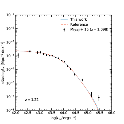
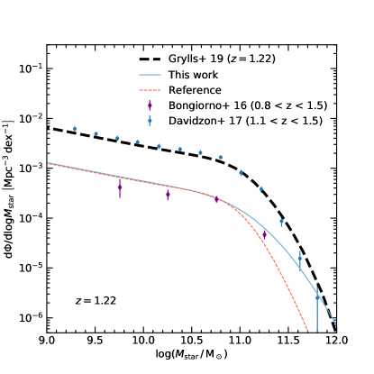
Figure 3: X-ray luminosity (left panel) and host galaxy stellar mass (right panel) functions of mock AGNs compared to data. Blue solid lines show the mock AGN X-ray (left) stellar mass (right) functions using our covariant scatter method i.e. This work, while red dashed lines show the functions using the reference method. In the right-hand side panel, we also show the mock non-active galaxy stellar mass function as a dashed line and for comparison the COSMOS galaxy/AGN host galaxy stellar mass functions of Davidzon et al. (2017, blue points) Bongiorno et al. (2016, purple diamonds). The AGN X-ray luminosity function at comparable redshift from Miyaji et al. (2015) (black points), are shown for reference.

In this work we implement two different methods to include the scatter in the input scaling relations. In the Reference case, for a given halo, we first assign the stellar mass following the ${M_{\mathrm{star}}}-{M_{\mathrm{halo}}}$ inclusive of the scatter. Then, we use the scattered galaxy stellar mass to assign the black hole mass given ${M_{\mathrm{BH}}}({M_{\mathrm{star}}})$

$$\log{M_{\mathrm{star}}} =\overline{\log M_{\mathrm{star}}}({\log M_{\mathrm{halo}}})+\delta\log{M_{\mathrm{star}}}$$ (1)

$$\log{M_{\mathrm{BH}}} =\overline{\log M_{\mathrm{BH}}}({\log M_{\mathrm{star}}})+\delta\log{M_{\mathrm{BH}}},$$ (2)

where $\delta\log{M_{\mathrm{star}}}$ is a Gaussian random variable with zero mean and a scatter of $0.11$ (Grylls et al., 2019) and $\delta\log{M_{\mathrm{BH}}}$ is a Gaussian random variable with ${M_{\mathrm{star}}}$ dependent intrinsic scatter of $0.32-0.1\times[\log({M_{\mathrm{star}}}/M_{\odot})-12]$ as suggested by Shankar et al. (2016).

However, in the second approach (covariant scatter method, This Work), for a given ${M_{\mathrm{halo}}}$, we assign the stellar mass ${M_{\mathrm{star}}}$ and black hole mass ${M_{\mathrm{BH}}}$ using the mean scaling relation for both properties. The multivariate normal scatter in ${M_{\mathrm{star}}}$ and ${M_{\mathrm{BH}}}$ is then assigned according to a given covariance matrix:

$$\left[\begin{matrix}\log{M_{\mathrm{star}}}\\ \log{M_{\mathrm{BH}}}\end{matrix}\right]=\left[\begin{matrix}\overline{\log M_{\mathrm{star}}}({\log M_{\mathrm{halo}}})\\ \overline{\log M_{\mathrm{BH}}}(\overline{\log M_{\mathrm{star}}})\end{matrix}\right]+\mathcal{N}\left(\mathbf{0},\mathbf{C}\right),$$ (3)

where $\mathcal{N}$ is the 2-dimensional Gaussian distribution with covariance matrix $\mathbf{C}$ (with covariances $C$)

$$\mathbf{C}=\left[\begin{matrix}C({\log{M_{\mathrm{star}}}},\log{M_{\mathrm{star}}})&C({\log{M_{\mathrm{star}}},\log{M_{\mathrm{BH}}}})\\ C({\log{M_{\mathrm{star}}},\log{M_{\mathrm{BH}}}})&C({\log{M_{\mathrm{BH}}},\log{M_{\mathrm{BH}}}})\end{matrix}\right],$$ (4)

Since data are sparse in terms of the covariance between ${M_{\mathrm{star}}}$ and ${M_{\mathrm{BH}}}$ for a given DM halo mass ${M_{\mathrm{halo}}}$ for AGNs, we use a local galaxy sample to derive the full covariance matrix by using the galaxy velocity dispersion and $K$-band luminosities as proxies of ${M_{\mathrm{halo}}}$ and ${M_{\mathrm{star}}}$, respectively.

We use the most updated local galaxy sample from de Nicola et al. (2019) which includes $84$ galaxies with black hole masses measured either from stellar dynamics, gas dynamics, or astrophysical masers, velocity dispersion and K-band luminosities. In this work our interest lies in the massive end of the DM halo mass function, and given that the AGN duty cycle is not well constrained for BHs with masses below $10^{6}\,\mathrm{M}_{\odot}$ (Schulze et al., 2015), we de-select potential low-mass systems by including only galaxies with velocity dispersion $\sigma>10^{2.1}\,\mathrm{km}/\mathrm{s}$, leaving $71$ galaxies in our final sample, which we show in the left and right panels of Fig. 2.

Our approach is outlined as follows. We start by re-evaluating the scaling scatter and the full covariance matrix for the scaling relations of the local galaxy sample of de Nicola et al. (2019). We use the K-band luminosity $L_{\mathrm{K}}$ and velocity dispersion $\sigma$ as proxies of ${M_{\mathrm{star}}}$ and ${M_{\mathrm{halo}}}$, in log-linear scale. We then estimate the ${M_{\mathrm{BH}}}$–$\sigma$ and ${L_{\mathrm{K}}}$–$\sigma$ scaling relations, from which we calculate the scatter and the covariance of ${M_{\mathrm{BH}}}$ and ${{M_{\mathrm{star}}}}$ for a given ${M_{\mathrm{halo}}}$.

For fitting the scaling relations, we use the Bayesian linmix routine (Kelly, 2007), assuming:

$${l_{\mathrm{K}}}+\Delta{l_{\mathrm{K}}} =\alpha_{L_{\mathrm{K}}}+\beta_{L_{\mathrm{K}}}(s+\Delta s)+\epsilon_{L_{\mathrm{K}}}$$ (5)

$${m_{\mathrm{BH}}}+\Delta{m_{\mathrm{BH}}} =\alpha_{M_{\mathrm{BH}}}+\beta_{M_{\mathrm{BH}}}(s+\Delta s)+\epsilon_{M_{\mathrm{BH}}},$$ (6)

where $l_{\mathrm{K}}=\log{L_{\mathrm{K}}}$, $m_{\mathrm{BH}}=\log{M_{\mathrm{BH}}}$, and $s=\log\sigma$.

The observational errors, prefixed by $\Delta$ in the equation, are assumed to be drawn from a multivariate gaussian distribution with a negligible covariance between the errors (Saglia et al., 2016; van den Bosch, 2016). The intrinsic scatters $\epsilon$ are assumed to be drawn from normal distributions with zero means and $\sigma^{2}$ variance. We assume uninformative priors and do not mask the data, and use $20\,000$ Monte Carlo (MC) samples. We then derive the scatter (denoted by a prefixed $\delta$) from the log-linear relation for each MC sample $i=1-20\,000$ and for each observation $j=1-71$ from the log-linear relations:

$$\delta{l_{\mathrm{K,i,j}}} ={l_{\mathrm{K,j}}}-(\alpha_{L_{\mathrm{K,i}}}+\beta_{L_{\mathrm{K,i}}}s_{j}),$$ (7)

$$\delta{m_{\mathrm{BH,i,j}}} ={m_{\mathrm{BH,j}}}-(\alpha_{M_{\mathrm{BH,i}}}+\beta_{M_{\mathrm{BH,i}}}s_{j}).$$ (8)

Finally, we estimate the covariance from the scatter for each of the $i$ sample as follows (Farahi et al., 2019):

$$C_{i}({\log L_{\mathrm{K}}},\log{L_{\mathrm{K}}}) =\frac{1}{N-1}\sum_{j=1}^{N}\delta l_{\mathrm{K,i,j}}^{2},$$ (9)

$$C_{i}({\log M_{\mathrm{BH}}},\log{M_{\mathrm{BH}}}) =\frac{1}{N-1}\sum_{j=1}^{N}\delta m_{\mathrm{BH,i,j}}^{2},$$ (10)

$$C_{i}({\log L_{\mathrm{K}}},\log{M_{\mathrm{BH}}}) =\frac{1}{N-1}\sum_{j=1}^{N}\delta l_{\mathrm{K,i,j}}\delta m_{\mathrm{BH,i,j}},$$ (11)

where $N$ is the number of observations For our local sample of $71$ galaxies, we report $16\%$, $50\%$, and $84\%$ percentiles of the $20\,000$ MC samples in Table 1, as well as Fig. 2. In detail, for the scaling relations we find $\alpha_{M_{\mathrm{BH}}}=-4.19$, $\beta_{M_{\mathrm{BH}}}=5.45$, $\alpha_{L_{\mathrm{K}}}=2.06$ and $\beta_{L_{\mathrm{K}}}=3.83$. For the covariance matrix, we find the $50\%$ percentiles $C(\log{L_{\mathrm{K}},\log{L_{\mathrm{K}}}})=0.21$, $C(\log{M_{\mathrm{BH}}},\log{M_{\mathrm{BH}}})=0.19$ and $C(\log{L_{\mathrm{K}}},\log{M_{\mathrm{BH}}})=0.07$, which as discussed previously, are also the values we utilize as the baseline for the full covariance between ${M_{\mathrm{star}}}$ and ${M_{\mathrm{BH}}}$ in the covariant scatter method. However, the covariant scatter derived here may be considered as an upper limit of the scatter in the input scaling relations. In building our AGN mock catalogs, we fix an upper limit to the scatter in the BH - stellar mass relation by requiring that the high-end tail ($M_{\mathrm{star}}\geq 10^{11.5}\,M_{\odot}$) of the galaxy stellar mass function at $z=1.22$ is not overproduced. This corresponds to a reduction of $\sigma_{\log M_{\mathrm{star}}}^{2}$ by $50\%$ (see Fig. 3).

quantity	$16\%$	$50\%$	$84\%$
$\alpha_{L_{\mathrm{K}}}$	1.13	2.06	3.00
$\beta_{L_{\mathrm{K}}}$	3.44	3.83	4.22
$\sigma^{2}_{L_{\mathrm{K}}}$	0.14	0.17	0.20
$\alpha_{M_{\mathrm{BH}}}$	-5.11	-4.19	-3.26
$\beta_{M_{\mathrm{BH}}}$	5.06	5.45	5.84
$\sigma^{2}_{M_{\mathrm{BH}}}$	0.13	0.16	0.20
$C\left({\log{L_{\mathrm{K}}},\log{L_{\mathrm{K}}}}\right)$	0.20	0.21	0.21
$C\left({\log{M_{\mathrm{BH}}},\log{M_{\mathrm{BH}}}}\right)$	0.18	0.19	0.19
$C\left({\log{L_{\mathrm{K}}},\log{M_{\mathrm{BH}}}}\right)$	0.07	0.07	0.08

Table 1: Results from the linmix routine for the quoted quantities derived from $20\,000$ MC samples.

2.3 Parameter Q

We also investigate the effect of increasing the relative probability of satellite BHs of being active. Formally, we define $Q=U_{\mathrm{sat}}/U_{\mathrm{cen}}$, where $U$ is the duty cycle and the subscripts ‘sat’ and ‘cen’ refer to satellite and central BHs, respectively. We can relate the fraction of central and satellite active BHs to the total fraction of active BHs $U$ via the relation (Shankar et al., 2020) $U_{\mathrm{cen}}({M_{\mathrm{BH}}})=U({M_{\mathrm{BH}}})N({M_{\mathrm{BH}}})/\left[N_{\mathrm{cen}}({M_{\mathrm{BH}}})+QN_{\mathrm{sat}}({M_{\mathrm{BH}}})\right]$ and $U_{\mathrm{sat}}({M_{\mathrm{BH}}})=QU_{\mathrm{cen}}({M_{\mathrm{BH}}})$, respectively. Here $N$ refers to the numbers of total/central/satellite BHs. In principle, the parameter $Q$ may not strictly be a constant but a function of stellar mass and/or environment. However, in the spirit of keeping a flexible and transparent semi-empirical approach, we will for simplicity keep $Q$ a constant (Shankar et al., 2020; Allevato et al., 2021).

It is important to stress that varying the value of $Q$ only modifies the relative contributions of central and satellite BHs, but it does not alter the total duty cycle $U$ and thus it does not spoil the match to the AGN luminosity function. The parameter $Q$ is related to the fraction of AGN in satellite halos $f_{\mathrm{sat}}^{\mathrm{AGN}}$ by the relation (Shankar et al., 2020)

$$Q=\frac{f_{\mathrm{sat}}^{\mathrm{AGN}}}{1-f_{\mathrm{sat}}^{\mathrm{AGN}}}\times\frac{1-f_{\mathrm{sat}}^{\mathrm{BH}}}{f_{\mathrm{sat}}^{\mathrm{BH}}}$$ (12)

where $f_{\mathrm{sat}}^{\mathrm{AGN}}$ is defined via summation over all DM halos $i$:

$$f_{\mathrm{sat}}^{\mathrm{AGN}}=\frac{\sum_{i}U_{\mathrm{sat},i}}{\sum_{i}\left(U_{\mathrm{sat},i}+U_{\mathrm{cen},i}\right)},$$ (13)

and

$$f_{\mathrm{sat}}^{\mathrm{BH}}=\frac{N_{\mathrm{sat}}}{N_{\mathrm{sat}}+N_{\mathrm{cen}}}$$ (14)

is the total fraction of (active and non active) BHs in satellites. In this work we will study how the $Q$ parameter affects AGN clustering estimates, and in particular the AGN $b({M_{\mathrm{star}}})$.

2.4 Mock AGN samples

For a closer comparison between our semi-empirical models and observations, we match our AGN simulated mocks to the observed samples in terms of $L_{\mathrm{X}}$ and stellar mass distributions. We also add to the intrinsic scatter in the stellar mass – halo mass relation, a measurement error of $0.20\,\mathrm{dex}$ to better reproduce the observed scatter in the stellar mass estimates in the COSMOS AGN samples (Allevato et al., 2019; Viitanen et al., 2019). Our reference observed AGN samples are from XMM/Chandra-COSMOS (Allevato et al., 2019; Viitanen et al., 2019) and XMM-XXL (Mountrichas et al., 2019). Mountrichas et al. (2019) measured the large-scale bias as a function of host galaxy stellar mass of $407$ moderate luminosity X-ray selected AGN in the XMM-XXL survey at redshift $0.5<z<1.2$ (mean $L_{\mathrm{X}}=10^{43.7}\,\mathrm{erg}/\mathrm{s}$). Viitanen et al. (2019) measured large-scale bias of $632$ XMM-COSMOS moderate luminosity X-ray type 1 & 2 AGN at $0.1<z<2.5$ (mean $z\sim 1.2$) and mean $L_{\mathrm{X}}=10^{43.7}\,\mathrm{erg}/\mathrm{s}$. Finally, at similar luminosities, Allevato et al. (2019) measured with high accuracy the large-scale bias of $800$ X-ray AGN in the Chandra-COSMOS Legacy (CCL) Survey at $z\sim 1$.

In the following, we also compare with the AGN semi-empirical model of Aird & Coil (2021), for which we apply an X-ray luminosity cut at ${L_{\mathrm{X}}}>10^{42}$. Lastly, we compare our predictions with the clustering estimates of SDSS quasars at $z\sim 1.4$ measured by Richardson et al. (2012), and for this test we impose a limit on luminosity of ${L_{\mathrm{X}}}>10^{44}\,\mathrm{erg}\,\mathrm{s}^{-1}$ and on Hydrogen column density of ${N_{\mathrm{H}}}<10^{22}\,\mathrm{cm}^{-2}$ to select only optical, nominally Type I AGN (e.g., Ricci et al., 2017). We list some of the main features of each of our reference AGN mock subsample in Table 2.

sample	$N_{\mathrm{halo}}$	$N_{\mathrm{AGN}}$	$Q$	$f_{\mathrm{sat}}^{\mathrm{AGN}}$
Aird+ 21 -like	$5\,746\,229$	$1\,022\,468$	1.00	0.12
Aird+ 21 -like	$5\,768\,258$	$1\,026\,768$	2.00	0.22
Allevato+ 19 -like	$1\,459\,756$	$217\,799$	1.00	0.10
Allevato+ 19 -like	$1\,468\,620$	$219\,237$	2.00	0.18
Allevato+ 19 -like	$1\,454\,717$	$216\,930$	4.00	0.31
Allevato+ 19 -like	$1\,464\,559$	$218\,672$	6.00	0.40
Richardson+ 12 -like	$324\,580$	$27\,078$	1.00	0.07
Richardson+ 12 -like	$321\,187$	$26\,654$	4.00	0.23
Richardson+ 12 -like	$324\,981$	$26\,974$	6.00	0.31

Table 2: Properties of the AGN sub-samples used in this work. The columns correspond to the name of the sample, number of DM halos, number of AGN defined as the sum of the duty cycles, $Q$ parameter, and corresponding AGN satellite fraction. See the text for the details on the sample definitions.

2.5 Two-point correlation function and large-scale bias

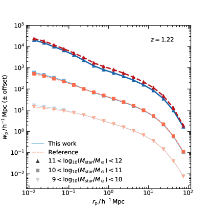
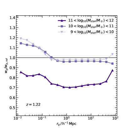
Figure 4: Left: projected correlation functions of mock AGNs in bins of host galaxy ${M_{\mathrm{star}}}$ assuming $Q=1$. Blue solid lines show the covariant scatter method, while red dashed lines show the reference case. Bins of ${M_{\mathrm{star}}}$ (in units of $\,\mathrm{M}_{\odot}$) are indicated by the symbols and the shades of color. For an easier comparison between the two methods, the lowest and the highest ${M_{\mathrm{star}}}$ bins have been offset in the direction of $w_{\mathrm{p}}$ by $-1$ and $+1$ dex, respectively. Right: the relative bias in $w_{\mathrm{p}}(r_{\mathrm{p}})$ using the two methods for the scatter. Different symbols indicate the different stellar mass bins following the legend.

For quantifying the clustering of mock AGNs, we use two complementary approaches. Firstly, we compute the projected two-point correlation function using the three-dimensional positions of the AGN host DM halos. Secondly, we calculate the AGN large-scale bias by averaging over the biased parent DM halo population.

We estimate the projected two-point correlation function of mock AGNs by using the 3-d positions of the hosting DM halos, following Davis & Peebles (1983):

$$w_{\mathrm{p}}(r_{\mathrm{p}})=2\times\int_{0}^{\pi_{\max}}\xi(r_{\mathrm{p}},\pi)\mathrm{d}\pi$$ (15)

where $\xi(r_{\mathrm{p}},\pi)$ is the 2-dimensional Cartesian two-point correlation function (e.g. Peebles, 1980). Physical distances $r_{\mathrm{p}}$ and $\pi$ correspond to the perpendicular and parallel (defined with respect to a far-away observer) separations, defined for each AGN pair $DD_{i,j}(r_{\mathrm{p}},\pi)$ separately. Using periodic boundary conditions in the simulation box with volume $V=10^{9}\,{({h}^{-1}\mathrm{Mpc})}^{3}$, $\xi(r_{\mathrm{p}},\pi)$ is estimated using

$$1+\xi(r_{\mathrm{p}},\pi) =\frac{DD(r_{\mathrm{p}},\pi)}{RR(r_{\mathrm{p}},\pi)},$$ (16)

$$DD(r_{\mathrm{p}},\pi) =\sum_{i,j}U_{i}\times U_{j},$$ (17)

$$RR(r_{\mathrm{p}},\pi) \approx\frac{\Delta V}{V}{\left(\sum_{k}U_{k}\right)}^{2}$$ (18)

where $DD$ is the sum of all unique mock AGN pairs $i,j$ within cylindrical volume element $\Delta V$ defined as the volume enclosed by $\log r_{\mathrm{p}}\pm\Delta\log r_{\mathrm{p}}/2$ and $\pi\pm\Delta\pi/2$ weighted by the AGN duty cycle $U$, and $RR$ is the expected number of randomly distributed mock AGN pairs within the same volume (e.g. Alonso, 2012; Sinha & Garrison, 2020). For estimating the correlation function, we use $r_{\mathrm{p}}=0.1-100\,{h}^{-1}\mathrm{Mpc}$, and $\pi=0-40$ ($\pi_{\max}=40\,{h}^{-1}\mathrm{Mpc}$) with bin sizes $\Delta\log(r_{\mathrm{p}}/\,{h}^{-1}\mathrm{Mpc})=0.25$ and $\Delta\pi=1\,{h}^{-1}\mathrm{Mpc}$, respectively. We use the publicly available CorrFunc code (Sinha & Garrison, 2020).

For the large-scale bias $b({M_{\mathrm{star}}})$ we estimate the bias for each DM halo separately. Halos are labeled as central or satellite. For each central halo, we assign a value of the large-scale bias according to van den Bosch (2002); Sheth et al. (2001). For each satellite DM halo we assign a large-scale bias value based on the mass of its parent halo, as each satellite traces the dense environment of the parent halo. Then, we follow the formalism of Shankar et al. (2020); Allevato et al. (2021) to derive the bias of mock AGN and normal galaxies as a function of galaxy stellar mass, by using the $Q$ parameter. The bias of mock objects with stellar mass in the range $M_{\mathrm{star}}\pm\mathrm{d}M_{\mathrm{star}}/2$ is estimated as a weighted average:

$$\begin{split}b({M_{\mathrm{star}}})&=\left[\sum_{i=1}^{N_{\mathrm{cen}}}U_{\mathrm{cen},i}(M_{\mathrm{star}})b_{\mathrm{cen},i}(M_{\mathrm{star}})\right.\\ &+\left.\sum_{i=1}^{N_{\mathrm{sat}}}U_{\mathrm{sat},i}(M_{\mathrm{star}})b_{\mathrm{sat},i}(M_{\mathrm{star}})\right]\\ &\left/\left[\sum_{i=1}^{N_{\mathrm{cen}}}U_{\mathrm{cen},i}(M_{\mathrm{star}})\right.\right.+\left.\sum_{i=1}^{N_{\mathrm{sat}}}U_{\mathrm{sat},i}(M_{\mathrm{star}})\right]\end{split}$$ (19)

When $Q=1$ and $U_{\mathrm{sat}}=U_{\mathrm{cen}}$, then on average central and satellite BHs share equal probabilities of being active.

3 Results

In this section we present our main results in terms of projected two-point correlation function $w_{\mathrm{p}}(r_{\mathrm{p}})$, AGN large-scale bias as a function of galaxy stellar mass $b({M_{\mathrm{star}}}$) and mean AGN halo occupation distribution (HOD) $\left\langle N(M_{\mathrm{halo}})\right\rangle$, i.e. the average number of AGN as a function of the halo mass. In what follows, we label as “This work” all results based on the covariant scatter method, while we use the “Reference” label for all models characterised by independent Gaussian scatters in all the input scaling relations.

The left panel of Fig. 4 shows the projected correlation function $w_{\mathrm{p}}(r_{\mathrm{p}})$ of mock AGNs created using the covariant scatter method (solid lines) and the reference model (dashed red lines), for different host galaxy stellar mass bins. The right panel of Fig. 4 plots instead the relative bias between the two different approaches. On large scales, the difference is in the highest stellar mass bin $11<\log{(M_{\mathrm{star}}/M_{\odot})}<12$, where the clustering strength of the covariant scatter is a factor of $\sim 0.7$ lower compared to the reference case. At smaller stellar masses, the two cases differ by a more moderate factor of $\lesssim 0.9$. Meanwhile, at lower scales $r_{\mathrm{p}}$, and for the lower stellar mass bins, we find an opposite trend, where the clustering strength of the covariant scatter case is higher by up to a factor of $\sim 1.2$.

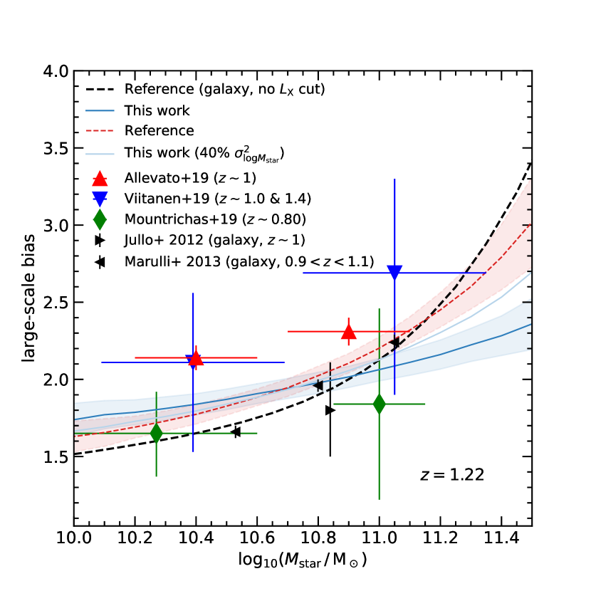
Figure 5: Large-scale bias as a function of the galaxy stellar mass of normal galaxies (black dashed line) compared to measurements of Jullo et al. (2012) and Marulli et al. (2013) (black left and right triangles); and mock AGNs when using the covariant scatter method, as solid (‘This work’) and dashed (‘Reference’) lines, respectively. The shaded region shows the 1$\sigma$ error of the AGN bias using a COSMOS-like volume (see the text for the details). The lighter blue line shows the effect of reducing the variance of the stellar mass for a given DM halo mass in the covariant scatter method to $40\%$ of the covariant scatter value. The markers show the X-ray AGN bias measurements from recent X-ray AGN clustering studies at similar redshifts (Allevato et al., 2019; Mountrichas et al., 2019; Viitanen et al., 2019) in accordance with the legend.

In Fig. 5 we show the bias in bins of stellar mass of mock AGNs for the covariant scatter case (solid blue line), and the reference case (dashed red line), and for X-ray selected AGN at $z\sim 1$ (Allevato et al., 2019; Mountrichas et al., 2019; Viitanen et al., 2019). For these comparisons, we match the mock AGN sample in terms of X-ray luminosity to the Chandra-COSMOS sample (Allevato et al., 2019), as explained in Sec. 2.4. In the covariant scatter case, the predicted AGN bias is almost constant as a function of stellar mass, as the covariance by design tends to naturally increase the scatter in stellar mass at fixed DM halo mass. In fact, further decreasing the intrinsic scatter in stellar mass to $40\%$ of the value derived in the covariant scatter method, leads to an AGN large-scale bias that is closer to the reference case without covariance (dashed red line). Moreover, we note that the typical $M_{\mathrm{star}}$ measurement error in COSMOS (see Sec. 2) added on top of the intrinsic scatter bridges some of the gap in the difference of the biases at $M_{\mathrm{star}}\gtrsim 10^{11}\,M_{\odot}$, where the inclusion of this additional scatter lowers the bias at a given stellar mass principally in the reference case.

For completeness, we also show the large-scale bias as a function of stellar mass of VIPERS (Marulli et al., 2013) and COSMOS (Jullo et al., 2012) for all galaxies at a similar redshift, which is well reproduced by our mock galaxies (i.e., bias not weighted by the duty cycle and without cuts in the X-ray luminosity, black dashed line in Fig. 5). It is worth noticing that, in the reference case, normal and active galaxies with the same luminosity cut follow the same bias - stellar mass relation. A larger degree of discrepancy in the bias in bins of stellar mass between AGN and normal galaxies is instead predicted when assuming a covariant scatter, especially at $\log{(M_{\mathrm{star}}/M_{\odot})}>11$ (see Sec. 4 for more discussion).

The predicted bias as a function of stellar mass of mock AGNs is consistent with the bias estimates of X-ray selected AGN characterized by a large uncertainty, irrespective of the used method for the scatter. However, the bias of mock AGNs appears systematically below by at least $\sim 20\%$ the measurements derived in Allevato et al. (2019) for Chandra-COSMOS AGN.

There could be different, concurrent causes that could explain the offset between COSMOS and the mocks. The COSMOS field is renown to be characterized by overdensities at $z<1$ that might increase the AGN large-scale bias by up to 26% (e.g. Gilli et al., 2009; Mendez et al., 2016), and suffers from cosmic variance due to the small volume. In particular, to estimate the effect of such a finite volume in our AGN mocks, we provide an estimate of the cosmic variance by sampling the full MDPL2 simulation box with side length of 1 Gpc/h. We then extract a total of 36 unique sub-volumes with area $27\times 27$ ${(\mathrm{Mpc}/h)}^{2}$ approximately $1.4$ deg² at $z=1$, comparable to the COSMOS field (Scoville et al., 2007), and length 1 Gpc/h, and calculate the large-scale bias for each of the 36 sub-boxes individually. We then use the standard deviation of the large-scale bias from the sub-volumes as an estimate of the effect of the cosmic variance. The filled areas in Fig. 5 shows the $1\sigma$ error of the bias, upon selecting a COSMOS-like volume from the full MDPL2 simulation box, which is of the order of $\sim$0.1 dex at almost all stellar masses. Our results would thus imply that, by itself, cosmic variance cannot account for the full offset between our mocks and the Allevato et al. (2019) bias measurements. We will discuss additional factors that could contribute to the discrepancy between models and data in what follows below. We will specifically investigate the dependence of the AGN large-scale bias (and related AGN HOD) on other input parameters, namely the BH - galaxy scaling relation and the AGN satellite fraction (i.e., the number of AGN in massive galaxy groups/clusters) as parametrized by $Q$.

3.1 Dependence on Input Scaling Relations

Figure 6: Large-scale bias as a function of host galaxy stellar mass and its dependence on the input ${M_{\mathrm{BH}}}({M_{\mathrm{star}}})$ relation. The shaded area around Shankar et al. (2016) relation shows the bias weighted additionally by the probability of a galaxy of being quenched as a function of the DM halo mass and redshift (assuming $\mu=2.5$) as given by Zanisi et al. (2021). The limits correspond to AGN host galaxies consisting solely of quenched (upper limit), and non-quenched (lower limit) galaxies. Otherwise the symbols and linestyles are the same as in Fig. 5.

In the creation of AGN mock catalogs we have assigned black hole masses to galaxies according to their host galaxy stellar mass following Shankar et al. (2016). Here we explore the impact of varying this input relation. We adopt the relation derived by Savorgnan & Graham (2016) for a sample of galaxies with dynamically measured BH masses, as presented in Eq. 3 of Shankar et al. (2019), which predicts higher ${M_{\mathrm{BH}}}$ for a given ${M_{\mathrm{star}}}$. These two chosen relations broadly bracket the existing systematic uncertainties in the black hole mass–stellar mass relation of dynamically measured BHs in the local Universe, with other scaling relations broadly falling in between them (e.g., Terrazas et al., 2016; Davis et al., 2019; Sahu et al., 2019).

We find that, in the reference case, the AGN large-scale bias as a function of stellar mass is independent of the particular input BH mass – stellar mass relation. When assuming the covariant scatter method instead, the AGN bias predicted by the Savorgnan & Graham (2016) relation is slightly lower (by $\sim 0.1$ dex) at lower stellar masses as compared to assuming the relation proposed by Shankar et al. (2016).

In our model we also assume that AGNs reside in a mixed population of host galaxies, i.e. active BHs share the same probability of being active in star forming and quenched galaxies. We can relax this assumption and explore the effect on the AGN bias as a function of stellar mass of having all AGNs in quenched galaxies. To this purpose, we assign to each AGN a probability of being in a quenched host galaxy $f_{quench}$ as a function of halo mass and redshift following Rodríguez-Puebla et al. (2015) and Zanisi et al. (2021). In detail, we use $f_{\mathrm{quench}}=1/[b_{0}+(M(z,\mu)\times 10^{12}/M_{\mathrm{halo}})]$, where $M(z,\mu)=M_{0}+{(1+z)}^{\mu}$, with $M_{\mathrm{halo}}$ given in units of solar masses, $M_{0}=0.68$, $b\sim 1$, and $\mu\sim 2.5$ (see Zanisi et al. 2021 for the details). We note that variations in $\mu=1-4$ affect the large-scale bias at most at the $\sim 5\%$ level as compared to $\mu=2.5$. We show the result in Fig. 6 as a shaded area, where the upper (lower) limit corresponds to the AGN bias in bins of stellar mass when assuming all AGNs in quenched (non-quenched) galaxies. In particular, assuming that all mock AGNs reside in quenched host galaxies, which live preferentially in more massive and biased halos, produces a large-scale bias as a function of stellar mass slightly higher ($1.05$ times) than when considering AGN in a mixed population.

3.2 Dependence on Q

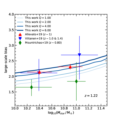
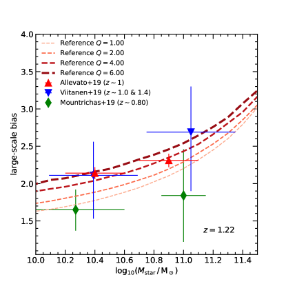
Figure 7: Large-scale bias as a function of stellar mass for different AGN satellite fractions parametrized by the $Q$ parameter. In the left (right) panel, different lines show the bias using the covariant scatter (reference) method with $Q=1-6$ as indicated by different line widths and colors.

In this section we study the effect of varying the relative number of satellite AGNs parameterized by $Q$. Fig. 7 shows that higher values of $Q$ tend to increase the normalization of the bias at all considered stellar masses, both in This Work and in the Reference case. This can be understood as an increase in the fraction of AGNs in highly biased massive systems, which are likely to host satellite AGNs in the first place. Increasing the probability of a satellite BHs being active thus increases the bias. We show this effect for moderate values of $Q=1,2$ (i.e. satellite BHs are $1-2$ times more likely to be active than centrals), but also more extreme values of $Q=4,6$. Bias estimates for X-ray selected COSMOS AGN seem to favour values of $Q\sim 4$, while XMM-XXL AGN are more in agreement with models with $Q=1$.

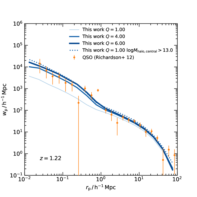
Figure 8: Projected correlation function including the 1-halo term ($r_{\mathrm{p}}\leq 1-2\,{h}^{-1}\mathrm{Mpc}$) of the QSO-like mock AGN sample (${L_{\mathrm{X}}}>10^{44}\,\mathrm{erg}\,\mathrm{s}^{-1}$, ${N_{\mathrm{H}}}<10^{22}\,\mathrm{cm}^{-2}$) compared to Richardson et al. (2012) SDSS QSOs at a similar redshift. The results are shown for the covariant scatter method, although there is no significant dependence on the method used.

We can convert any value of $Q$ to an actual fraction of satellite active BHs above a given luminosity threshold. Values of $Q=1,2,4,6$ correspond to AGN satellite fractions $f_{\mathrm{sat}}^{\mathrm{AGN}}=0.10,0.18,0.31,0.40$, respectively (see Table 2). In Fig. 9 we compare our predicted satellite fractions as a function of parent host DM halo mass for different $Q$ values, with models of Gatti et al. (2016) and Aird & Coil (2021) for AGNs with ${L_{\mathrm{X}}}>10^{42}\,\mathrm{erg}/\,\mathrm{s}$ and data from Pentericci et al. (2013) and Martini et al. (2009). Measurements of the AGN satellite fraction in groups and clusters (Pentericci et al., 2013; Martini et al., 2009) suggest small values of $Q\sim 1-2$, as also assumed in the semi-empirical model presented in Aird & Coil (2021). It is worth noticing that independently of the parameter $Q$, $f_{\mathrm{sat}}$ is by construction increasing as a function of the parent DM halo mass (see Fig. 9). In particular, higher $Q$ increases the AGN satellite fraction in less massive parent halos. Our results show that the AGN satellite fraction is thus an input parameter that controls the normalization of the AGN large-scale bias as a function of stellar mass. Additional measurements of $f_{\mathrm{sat}}$ in groups and clusters at this redshift would help in putting independent constraints on $Q$.

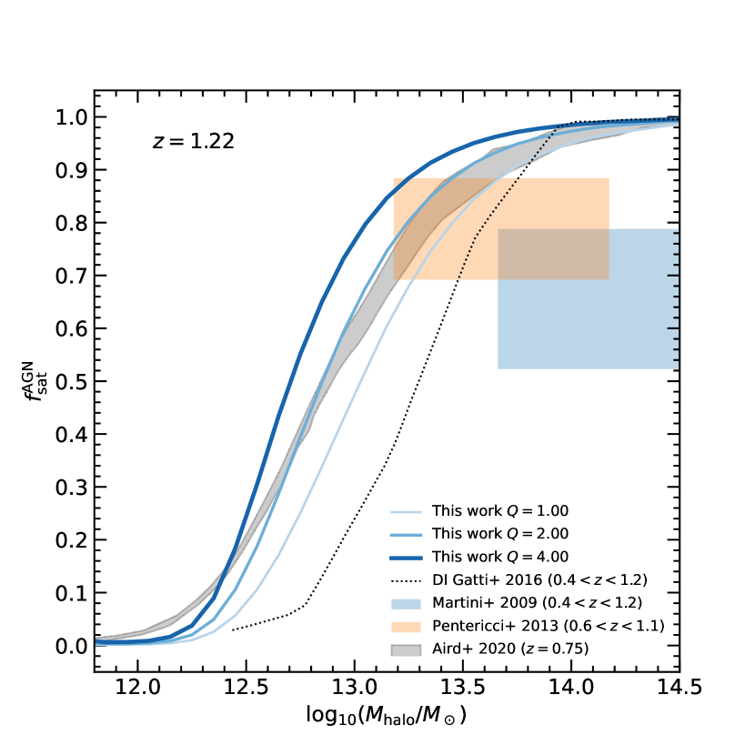
Figure 9: Fraction of satellite AGN as a function of parent host DM halo mass for different values of $Q$ parameter. Colored lines with increasing widths correspond to ascending values of $Q$ for our mock AGNs, while the shaded region shows the limiting values of Aird & Coil (2021) model. The semi-analytic model prediction of Gatti et al. (2016) based AGN triggering through disc instabilities (DI) is shown as a dark dotted line. Martini et al. (2009); Pentericci et al. (2013) show measurements of X-ray AGNs in galaxy groups/clusters.

3.3 AGN HOD and the 1-halo term

Finally, we estimate the projected two-point correlation function (2pcf) and corresponding mean halo occupation distribution (HOD) of mock AGNs. In particular, we measured the mock AGN 2pcf over the full scale range $r_{\mathrm{p}}=0.1-100\,{h}^{-1}\mathrm{Mpc}$ including the small scales within the 1-halo ($<1{h}^{-1}\mathrm{Mpc}$) which is due to the correlation of AGN within the same DM halo. This regime is especially sensitive to the fraction of AGNs in satellite galaxies of galaxy groups and clusters. The mock AGN HOD is calculated as the average number of mock AGNs in bins of DM halo mass, separating the contribution of mock satellite and central AGNs. Fig. 8 shows the 2pcf of mock AGNs with $L_{\mathrm{X}}>10^{44}\,\mathrm{erg}/\mathrm{s}$ and ${N_{\mathrm{H}}}<10^{22}\,\mathrm{cm}^{-2}$ for $Q=2,4$ and $6$, compared with the 2pcf estimated Richardson et al. (2012). The comparison with data suggests high values of $Q$ (= 4), with a corresponding satellite AGN fraction of $f_{\mathrm{sat}}^{\mathrm{AGN}}0.23$ (see Table 2).

The corresponding mean HODs of mock AGNs and SDSS quasars are shown if Fig. 10 (right panel). While the SDSS quasar HOD is characterized by a significant central occupation only for DM halos with $M_{\mathrm{halo}}>10^{13}\,M_{\odot}$ with a steep increase of the satellite quasar HOD as a function of the hosting halo mass, the occupation of our central mock AGNs is significant in halos with mass down to $M_{\mathrm{halo}}\sim 10^{12.3}h^{-1}M_{\odot}$. Moreover, the satellite fraction derived for SDSS quasars in Richardson et al. (2012) is $\sim 1000$ times smaller than the one measured in our AGN mock catalog. This comparison shows that AGN small scale clustering can be modelled by HODs characterized by different satellite AGN fractions and minimum mass of the hosting halos.

A similar result is also shown in the left panel, for mock AGN with $L_{\mathrm{X}}>10^{42}\,\mathrm{erg}/\mathrm{s}$, compared to the HOD derived in Richardson et al. (2013) for X-ray selected COSMOS AGN at $z\sim 1.2$. Also for moderate luminosity AGN, they found an upper limit of $f_{\mathrm{sat}}^{\mathrm{AGN}}=0.1$ and a significant central occupation for central halos with mass $M_{\mathrm{halo}}>10^{12}h^{-1}M_{\odot}$, i.e. almost 3 times larger than what derived from our mock AGNs. For comparison, we also show the AGN HOD from the semi-empirical model by Aird & Coil (2021), which is in fair agreement with our predictions (for $Q=1$), especially at large parent halo masses. Their model also finds a significant AGN HOD for hosting halos with mass down to $M_{\mathrm{halo}}>10^{11.5}h^{-1}M_{\odot}$.

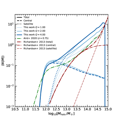
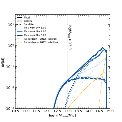
Figure 10: Halo occupation distribution of mock AGNs derived by counting the average number of active BHs in bins of parent halo mass in this work (in blue) and in empirical mocks of Aird & Coil (2021, in green); and as estimated in Richardson et al. (2013, left panel, in red) and Richardson et al. (2012, right panel, in yellow) modelling the 2pcf of COSMOS AGN and SDSS quasars. Total, central, and satellite occupations are shown by solid, dashed, and dotted lines, respectively. Different linewidths correspond to different input $Q$ values as indicated by the legend. In addition, in the right panel we indicate as a vertical line the position of the model with the central DM halo mass cut, as shown in Fig. 8.

4 Discussion

In this work we create realistic mock catalogs of active BHs and galaxies at $z\sim 1.2$ based on semi-empirical models, to study the impact on the AGN large-scale bias as a function of the host galaxy stellar mass and focus in particular on the impact of (1) including a covariant scatter in the BH mass – stellar mass relation at fixed halo mass; (2) changing the satellite AGN fraction. We demonstrate that the AGN bias at fixed stellar mass is mainly dependent on the scatter in the input scaling relations and on the relative fraction of satellite and central active BHs.

4.1 Covariant Scatter

The scatter in the input BH mass – stellar mass relation strongly affects the AGN large-scale bias as a function of stellar mass. In particular we found that the larger the scatter, the flatter is the resulting bias – stellar mass relation. This behaviour is expected as the end product of a covariant scatter is to generate a larger scatter in the input In detail, the covariant scatter model produces an AGN bias versus $M_{\mathrm{star}}$ up to twice as small at $M_{\mathrm{star}}\sim 10^{11.5}M_{\odot}$ than the Reference case. A model with covariant scatter, i.e. with a (positive) correlation between BH mass and galaxy mass at fixed halo mass, would then imply a bias as a function of stellar mass substantially different between AGN and the overall population of galaxies at the same stellar mass, at least for M${}_{\mathrm{star}}>10^{11}M_{\odot}$, where unfortunately AGN bias estimates are not yet available and/or still have large associated uncertainties (Mountrichas et al., 2019; Viitanen et al., 2019; Allevato et al., 2019). At $M_{\mathrm{star}}<10^{11}\,M_{\odot}$, instead, the difference in the large-scale bias of normal and active galaxies at the same stellar mass is not significant, as also found in Mendez et al. (2016) and Powell et al. (2018).

Our predicted AGN large-scale bias is roughly consistent with the measurements by (Mountrichas et al., 2019; Viitanen et al., 2019), which are however characterized by large uncertainties, but it always falls short by a systematic $\sim 20\%$ in reproducing the measured bias of CCL AGNs (Allevato et al., 2019), at least for models with $Q=1$. The COSMOS field (Scoville et al., 2007) is known to be characterized by large overdensities at $z<1$ which could increase the large-scale bias up to $\sim 20-50\%$ (Gilli et al., 2009; Mendez et al., 2016; Viitanen et al., 2019). In fact, Viitanen et al. (2019) also estimate the AGN bias when removing from the sample AGN in galaxy groups and measured a bias $\sim$0.4 dex smaller in the lower stellar mass bin. In addition, the COSMOS field is affected by cosmic variance due to the small volume of the survey which introduces an additional $1\sigma$ error of $\sim$0.1 dex to the bias measurements (see Sec.3 for more details). All these effects make it difficult to constrain models with and without covariant scatter. In the near future, precise clustering measurements of AGN that extend up to $M_{\mathrm{star}}>10^{11}M_{\odot}$ will allow us to put constraints on these models.

The study of the degeneracy between AGN clustering strength and scatter in the BH–host scaling relations has already been emphasized by a number of groups at different redshifts (e.g., Shen et al., 2007; White et al., 2008; Wyithe & Loeb, 2009; Bonoli et al., 2010; Shankar et al., 2010b; Shankar et al., 2010a). One of the main findings emphasised by these studies was the need for a small scatter in the input scaling relation to boost the AGN clustering signal to match some of the data. Our current results point to similar trends, whilst emphasizing the vital role of additional parameters, such as the relative fraction of AGN satellites, in amplifying the clustering signal.

4.2 Satellite AGN fraction

In this work we have highlighted the pivotal role of the $Q$ parameter, i.e. the ratio between active satellite and central BHs, in regulating the normalization of the bias–stellar mass relation (e.g., Figure 7). In addition, constraining the $Q$ parameter can shed light on AGN triggering models. For example, a high relative fraction of satellite AGN would be in line with the evidence put forward several times that secular processes and bar instabilities, and not only mergers (e.g., Hopkins et al., 2008), are efficient in triggering moderate-to-luminous AGN (e.g. Georgakakis et al., 2009; Allevato et al., 2011; Cisternas et al., 2011a; Schawinski et al., 2011; Rosario et al., 2011).

The value of $Q$ is yet not well constrained at $z>1$, whilst most studies suggest that $Q\lesssim 2$ at $z\geq 1$. Allevato et al. (2019) suggested that the $z\sim 1$ large-scale bias of CCL Type 2 AGN as a function of the host galaxy stellar mass can be reproduced assuming $Q\sim$ 2, which corresponds to a satellite AGN fraction $f_{\mathrm{AGN}}^{\mathrm{sat}}\sim 0.15$, and applying a cut in the AGN host halo mass of $M_{\mathrm{halo}}\gtrsim 10^{12}h^{-1}M_{\odot}$. Estimates of the AGN content in groups of galaxies in the two GOODS fields at $z\sim 1$ (Pentericci et al., 2013) favour $Q\sim 1-2$. At smaller redshifts, an AGN satellite fraction $f_{\mathrm{AGN}}^{\mathrm{sat}}\sim 0.18$ has been suggested by Leauthaud et al. (2015) for COSMOS AGN at $z<1$. Allevato et al. (2012) performed direct measurements of the HOD for COSMOS AGN at $z<0.2$ based on the mass function of galaxy groups hosting AGN, and found that the duty cycle of satellite AGN is comparable or slightly larger than that of central AGN, i.e. $Q\leq 2$. Georgakakis et al. (2019) used semi-empirical models to populate DM halos with AGN assuming no distinction between centrals and satellites, i.e. $Q=1$ and found a fair agreement, within the error budget, between the observationally derived AGN HOD (e.g. Allevato et al., 2012; Miyaji et al., 2011; Shen et al., 2013) and their AGN mock predictions. Shankar et al. (2020) also showed that the large-scale bias as a function of BH mass of X-ray and optically selected AGN at $z\sim 0.25$ can be reproduced by assuming $Q\leq$ 2. Recently, Allevato et al. (2021) showed that the Q parameter strongly affects the large-scale AGN bias as a function of stellar mass, BH mass and luminosity, with $Q\sim 1-2$ more favoured by the data at $z\sim 0.1$.

We also investigated how the $Q$ parameter affects the AGN HOD and in turn the 1-halo term. The HOD approach has been used by different authors to interpret AGN and quasar clustering measurements (e.g. Allevato et al., 2011; Miyaji et al., 2011; Richardson et al., 2012, 2013; Kayo & Oguri, 2012). In particular, Richardson et al. (2012) and Kayo & Oguri (2012) performed clustering measurements of optically luminous quasars for both small ($<1\,{h}^{-1}\mathrm{Mpc}$) and large physical scales and performed HOD modelling to infer the relation between quasars and their host dark matter halos (see Fig. 10). Richardson et al. (2012) found at $z\sim 1.4$ a small fraction of luminous SDSS quasars to be in satellites DM halos, with $f_{\mathrm{sat}}^{\mathrm{AGN}}\sim 7.4\times 10^{-4}$ and that the central (satellite) occupation becomes significant only at masses above $M_{\mathrm{halo}}\sim 10^{13}h^{-1}M_{\odot}$ ($\sim 10^{14}h^{-1}M_{\odot}$). Kayo & Oguri (2012) also modelled the clustering of SDSS quasars at $z\sim 1.4$ and reported a satellite fraction $\sim$100 times higher than Richardson et al. (2012), by using a different HOD parameterization. We also showed that by increasing the input $Q$ parameter we were able to reproduce the full 2pcf of luminous SDSS quasars with resulting HODs very different from those derived by Richardson et al. (2012), further highlighting the degeneracies in HOD modelling. We note that such degeneracies have already been reported from HOD modeling for SDSS the quasar two-point cross-correlation function at intermediate redshifts $0.3<z<0.9$ (Shen et al., 2013).

4.3 Alternatives to high Q values

The comparison of our mock predictions with the 2pcf at all scales of SDSS quasars suggest high values of $Q$ ($\sim$4), which are in contrast with previous measurements from HOD modelling in Richardson et al. (2012) and Kayo & Oguri (2012) and previous findings at lower $z$ (e.g. Leauthaud et al., 2012; Allevato et al., 2012). There could be various and concomitant causes that could determine this offset. An explanation could be that the MultiDark simulations used to create the AGN mock catalogs are characterized by missing satellite halos possibly due to the low mass resolution ($1.5\times 10^{9}h^{-1}M_{\odot}$) and/or stripped halos. Another possibility is that luminous quasars do not reside in central DM halos with mass $M_{\mathrm{halo}}<10^{13}h^{-1}M_{\odot}$ as suggested by the HOD modelling of Richardson et al. (2012). In fact, as shown in Fig. 8, the 2pcf (including the 1-halo term) of SDSS quasars can be easily reproduced by mock AGNs with $Q=1$ and applying a cut in the minimum mass of central AGN hosting halos at $M_{\mathrm{halo}}\sim 10^{13}h^{-1}M_{\odot}$. Similarly, one might expect that the bias estimates as a function of stellar mass for COSMOS AGN (Allevato et al., 2019; Viitanen et al., 2019) can also be reproduced assuming smaller $Q$ ($\sim$1) and a minimum mass in the central halos of $M_{\mathrm{halo}}\sim 10^{12}h^{-1}M_{\odot}$ (following Richardson et al., 2013).

These results suggest that the minimum central AGN hosting halo mass and $f_{\mathrm{sat}}$ are degenerate. The smaller the AGN satellite fraction is, the higher the mass needed for a central halo to host an AGN above a given luminosity. Moreover, the smaller $f_{\mathrm{sat}}$, the steeper is the increase of the satellite AGN occupation as a function of the parent halo mass. It is certain that a fraction of quasars must be satellites to produce the small-scale clustering of AGN. Currently available satellite AGN fraction estimates in groups and clusters of galaxies presented by Martini et al. (2009) and Pentericci et al. (2013) at $z\leq 1$ suggest small values of $Q$. Additional independent measurements of the AGN satellite fraction in groups and clusters at $z\geq 1$ would help in breaking the degeneracy in these model parameters.

5 Conclusions

Numerous degeneracies in the input parameters of cosmological models still prevent solid progress on the open issue of the co-evolution of supermassive black holes (BHs) and their host galaxies and dark matter halos. Building on previous work from our group and by making use of advanced and diverse semi-empirical routines, also inclusive of the covariance among some input parameters, we here show that:

• The overall shape and normalization of the large-scale bias as a function of AGN host galaxy stellar mass $b(M_{\mathrm{star}})$, is largely independent of the input stellar mass – halo mass relation, duty cycle and Eddington ratio distribution, while it is mostly driven by the dispersion in – not so much by the shape of – the input stellar mass–black hole mass relation.

• A model with covariant scatter, i.e. with a (positive) correlation between BH mass and galaxy mass at fixed halo mass, predicts an AGN bias almost independent of the stellar mass and substantially different from the bias of the underlying population of galaxies of the same stellar mass, at least in the range $M_{\mathrm{star}}>10^{11}M_{\odot}$. Present AGN clustering estimates at $z\sim 1.2$ do not allow us to clearly distinguish between models with and without a covariant scatter.

• The other parameter controlling the normalization of the AGN bias $b(M_{\mathrm{star}})$ is $Q$, the relative fraction of AGN hosted in satellite and central BHs of a given mass. Increasing the probability of AGN to be hosted in satellites rather than in centrals of equal BH mass, naturally increases the large-scale clustering as the bias becomes more heavily weighted towards more massive host halos.

• The comparison with the large-scale bias of COSMOS AGN at $z\sim 1.2$ and with the two-point correlation function of SDSS quasars at $z\sim 1.4$, suggests $Q\sim 4$ which corresponds to a relative fraction of AGN hosted in satellites $f_{\mathrm{sat}}^{\mathrm{AGN}}\sim 0.2-0.3$. However, the data are also reproduced by models that adopt $Q\leq 2$, i.e. values more consistent with independent estimates at the AGN fraction at lower z, as long as a cut is applied in the minimum mass of central AGN hosting halos, as also suggested by the HOD modelling in some clustering studies. This result unveils a strong degeneracy between the AGN satellite fraction and the minimum halo mass hosting AGN above a given luminosity. Independent estimates of the fraction of active satellites in groups at $z\geq 1$ will help in breaking this degeneracy.

In the next years, current and imminent extragalactic surveys, such as Euclid, eROSITA and LSST will precisely measure the clustering AGN at different masses and redshifts allowing to set invaluable constraints on many important features of AGN demography, such as limits on the covariance between AGN and galaxies, on the minimum halo mass hosting AGN, on the relative fraction of AGN satellites, and several others which will in turn provide essential constraints on the still puzzling co-evolution of BHs and their host galaxies and dark matter halos.

Data Availability

The MultiDark ROCKSTAR halo catalogues are available in the CosmoSim database at https://www.cosmosim.org/. Other data underlying this article will be shared on reasonable request to the corresponding author.

References

- Aird & Coil (2021) Aird J., Coil A. L., 2021, MNRAS, 502, 5962
- Aird et al. (2017) Aird J., Coil A. L., Georgakakis A., 2017, MNRAS, 465, 3390
- Allevato et al. (2011) Allevato V., et al., 2011, ApJ, 736, 99
- Allevato et al. (2012) Allevato V., et al., 2012, ApJ, 758, 47
- Allevato et al. (2019) Allevato V., et al., 2019, A&A, 632, A88
- Allevato et al. (2021) Allevato V., Shankar F., Marsden C., Rasulov U., Viitanen A., Georgakakis A., Ferrara A., Finoguenov A., 2021, arXiv e-prints, p. arXiv:2105.02883
- Alonso (2012) Alonso D., 2012, arXiv e-prints, p. arXiv:1210.1833
- Aversa et al. (2015) Aversa R., Lapi A., de Zotti G., Shankar F., Danese L., 2015, ApJ, 810, 74
- Bandara et al. (2009) Bandara K., Crampton D., Simard L., 2009, ApJ, 704, 1135
- Behroozi et al. (2013) Behroozi P. S., Wechsler R. H., Wu H.-Y., 2013, ApJ, 762, 109
- Behroozi et al. (2019) Behroozi P., Wechsler R. H., Hearin A. P., Conroy C., 2019, MNRAS, 488, 3143
- Bernardi (2007) Bernardi M., 2007, AJ, 133, 1954
- Bongiorno et al. (2012) Bongiorno A., et al., 2012, MNRAS, 427, 3103
- Bongiorno et al. (2016) Bongiorno A., et al., 2016, A&A, 588, A78
- Bonoli et al. (2010) Bonoli S., Shankar F., White S. D. M., Springel V., Wyithe J. S. B., 2010, MNRAS, 404, 399
- Cisternas et al. (2011a) Cisternas M., et al., 2011a, ApJ, 726, 57
- Cisternas et al. (2011b) Cisternas M., et al., 2011b, ApJ, 741, L11
- Coil et al. (2009) Coil A. L., et al., 2009, ApJ, 701, 1484
- Davidzon et al. (2017) Davidzon I., et al., 2017, A&A, 605, A70
- Davis & Peebles (1983) Davis M., Peebles P. J. E., 1983, ApJ, 267, 465
- Davis et al. (2019) Davis B. L., Graham A. W., Cameron E., 2019, ApJ, 873, 85
- Eisenstein & Hu (1998) Eisenstein D. J., Hu W., 1998, ApJ, 496, 605
- Fanidakis et al. (2012) Fanidakis N., et al., 2012, MNRAS, 419, 2797
- Farahi et al. (2019) Farahi A., et al., 2019, Nature Communications, 10, 2504
- Ferrarese (2002) Ferrarese L., 2002, ApJ, 578, 90
- Ferrarese & Ford (2005) Ferrarese L., Ford H., 2005, Space Sci. Rev., 116, 523
- Gatti et al. (2016) Gatti M., Shankar F., Bouillot V., Menci N., Lamastra A., Hirschmann M., Fiore F., 2016, MNRAS, 456, 1073
- Georgakakis et al. (2009) Georgakakis A., et al., 2009, MNRAS, 397, 623
- Georgakakis et al. (2014) Georgakakis A., et al., 2014, MNRAS, 443, 3327
- Georgakakis et al. (2017) Georgakakis A., Aird J., Schulze A., Dwelly T., Salvato M., Nandra K., Merloni A., Schneider D. P., 2017, MNRAS, 471, 1976
- Georgakakis et al. (2019) Georgakakis A., Comparat J., Merloni A., Ciesla L., Aird J., Finoguenov A., 2019, MNRAS, 487, 275
- Gilli et al. (2009) Gilli R., et al., 2009, A&A, 494, 33
- Graham & Scott (2015) Graham A. W., Scott N., 2015, ApJ, 798, 54
- Granato et al. (2004) Granato G. L., De Zotti G., Silva L., Bressan A., Danese L., 2004, ApJ, 600, 580
- Grylls et al. (2019) Grylls P. J., Shankar F., Zanisi L., Bernardi M., 2019, MNRAS, 483, 2506
- Hickox et al. (2009) Hickox R. C., et al., 2009, ApJ, 696, 891
- Hirschmann et al. (2010) Hirschmann M., Khochfar S., Burkert A., Naab T., Genel S., Somerville R. S., 2010, MNRAS, 407, 1016
- Hopkins et al. (2008) Hopkins P. F., Hernquist L., Cox T. J., Kereš D., 2008, ApJS, 175, 356
- Jahnke & Macciò (2011) Jahnke K., Macciò A. V., 2011, ApJ, 734, 92
- Jullo et al. (2012) Jullo E., et al., 2012, ApJ, 750, 37
- Kayo & Oguri (2012) Kayo I., Oguri M., 2012, MNRAS, 424, 1363
- Kelly (2007) Kelly B. C., 2007, ApJ, 665, 1489
- Klypin et al. (2016) Klypin A., Yepes G., Gottlöber S., Prada F., Heß S., 2016, MNRAS, 457, 4340
- Kormendy & Ho (2013) Kormendy J., Ho L. C., 2013, ARA&A, 51, 511
- Krumpe et al. (2010) Krumpe M., Miyaji T., Coil A. L., 2010, ApJ, 713, 558
- Krumpe et al. (2012) Krumpe M., Miyaji T., Coil A. L., Aceves H., 2012, ApJ, 746, 1
- Leauthaud et al. (2012) Leauthaud A., et al., 2012, ApJ, 744, 159
- Leauthaud et al. (2015) Leauthaud A., et al., 2015, MNRAS, 446, 1874
- Madau & Dickinson (2014) Madau P., Dickinson M., 2014, ARA&A, 52, 415
- Marconi et al. (2004) Marconi A., Risaliti G., Gilli R., Hunt L. K., Maiolino R., Salvati M., 2004, MNRAS, 351, 169
- Marsden et al. (2020) Marsden C., Shankar F., Ginolfi M., Zubovas K., 2020, Frontiers in Physics, 8, 61
- Martini et al. (2009) Martini P., Sivakoff G. R., Mulchaey J. S., 2009, ApJ, 701, 66
- Marulli et al. (2013) Marulli F., et al., 2013, A&A, 557, A17
- Mendez et al. (2016) Mendez A. J., et al., 2016, ApJ, 821, 55
- Miyaji et al. (2011) Miyaji T., Krumpe M., Coil A. L., Aceves H., 2011, ApJ, 726, 83
- Miyaji et al. (2015) Miyaji T., et al., 2015, ApJ, 804, 104
- Moster et al. (2010) Moster B. P., Somerville R. S., Maulbetsch C., van den Bosch F. C., Macciò A. V., Naab T., Oser L., 2010, ApJ, 710, 903
- Mountrichas & Georgakakis (2012) Mountrichas G., Georgakakis A., 2012, MNRAS, 420, 514
- Mountrichas et al. (2019) Mountrichas G., Georgakakis A., Georgantopoulos I., 2019, MNRAS, 483, 1374
- Peebles (1980) Peebles P. J. E., 1980, The large-scale structure of the universe. Princeton University Press
- Pentericci et al. (2013) Pentericci L., et al., 2013, A&A, 552, A111
- Powell et al. (2018) Powell M. C., et al., 2018, ApJ, 858, 110
- Powell et al. (2020) Powell M. C., Urry C. M., Cappelluti N., Johnson J. T., LaMassa S. M., Ananna T. T., Kollmann K. E., 2020, ApJ, 891, 41
- Reines & Volonteri (2015) Reines A. E., Volonteri M., 2015, ApJ, 813, 82
- Ricci et al. (2017) Ricci F., Marchesi S., Shankar F., La Franca F., Civano F., 2017, MNRAS, 465, 1915
- Richardson et al. (2012) Richardson J., Zheng Z., Chatterjee S., Nagai D., Shen Y., 2012, ApJ, 755, 30
- Richardson et al. (2013) Richardson J., Chatterjee S., Zheng Z., Myers A. D., Hickox R., 2013, ApJ, 774, 143
- Riebe et al. (2013) Riebe K., et al., 2013, Astronomische Nachrichten, 334, 691
- Rodríguez-Puebla et al. (2015) Rodríguez-Puebla A., Avila-Reese V., Yang X., Foucaud S., Drory N., Jing Y. P., 2015, ApJ, 799, 130
- Rosario et al. (2011) Rosario D. J., McGurk R. C., Max C. E., Shields G. A., Smith K. L., Ammons S. M., 2011, ApJ, 739, 44
- Saglia et al. (2016) Saglia R. P., et al., 2016, ApJ, 818, 47
- Sahu et al. (2019) Sahu N., Graham A. W., Davis B. L., 2019, ApJ, 876, 155
- Savorgnan & Graham (2016) Savorgnan G. A. D., Graham A. W., 2016, ApJS, 222, 10
- Schawinski et al. (2011) Schawinski K., Treister E., Urry C. M., Cardamone C. N., Simmons B., Yi S. K., 2011, ApJ, 727, L31
- Schulze et al. (2015) Schulze A., et al., 2015, MNRAS, 447, 2085
- Scoville et al. (2007) Scoville N., et al., 2007, ApJS, 172, 1
- Shankar et al. (2004) Shankar F., Salucci P., Granato G. L., De Zotti G., Danese L., 2004, MNRAS, 354, 1020
- Shankar et al. (2009a) Shankar F., Weinberg D. H., Miralda-Escudé J., 2009a, ApJ, 690, 20
- Shankar et al. (2009b) Shankar F., Bernardi M., Haiman Z., 2009b, ApJ, 694, 867
- Shankar et al. (2010a) Shankar F., Weinberg D. H., Shen Y., 2010a, MNRAS, 406, 1959
- Shankar et al. (2010b) Shankar F., Crocce M., Miralda-Escudé J., Fosalba P., Weinberg D. H., 2010b, ApJ, 718, 231
- Shankar et al. (2013) Shankar F., Weinberg D. H., Miralda-Escudé J., 2013, MNRAS, 428, 421
- Shankar et al. (2016) Shankar F., et al., 2016, MNRAS, 460, 3119
- Shankar et al. (2019) Shankar F., et al., 2019, MNRAS, 485, 1278
- Shankar et al. (2020) Shankar F., et al., 2020, Nature Astronomy, 4, 282
- Shen et al. (2007) Shen Y., et al., 2007, AJ, 133, 2222
- Shen et al. (2013) Shen Y., et al., 2013, ApJ, 778, 98
- Shen et al. (2015) Shen Y., et al., 2015, ApJ, 805, 96
- Sheth et al. (2001) Sheth R. K., Mo H. J., Tormen G., 2001, MNRAS, 323, 1
- Silk & Rees (1998) Silk J., Rees M. J., 1998, A&A, 331, L1
- Sinha & Garrison (2020) Sinha M., Garrison L. H., 2020, MNRAS, 491, 3022
- Suh et al. (2020) Suh H., Civano F., Trakhtenbrot B., Shankar F., Hasinger G., Sand ers D. B., Allevato V., 2020, ApJ, 889, 32
- Terrazas et al. (2016) Terrazas B. A., Bell E. F., Henriques B. M. B., White S. D. M., Cattaneo A., Woo J., 2016, ApJ, 830, L12
- Ueda et al. (2014) Ueda Y., Akiyama M., Hasinger G., Miyaji T., Watson M. G., 2014, ApJ, 786, 104
- Viitanen et al. (2019) Viitanen A., Allevato V., Finoguenov A., Bongiorno A., Cappelluti N., Gilli R., Miyaji T., Salvato M., 2019, A&A, 629, A14
- White et al. (2008) White M., Martini P., Cohn J. D., 2008, MNRAS, 390, 1179
- Wyithe & Loeb (2009) Wyithe J. S. B., Loeb A., 2009, MNRAS, 395, 1607
- Zanisi et al. (2021) Zanisi L., et al., 2021, MNRAS, 505, 4555
- de Nicola et al. (2019) de Nicola S., Marconi A., Longo G., 2019, MNRAS, 490, 600
- van den Bosch (2002) van den Bosch F. C., 2002, MNRAS, 331, 98
- van den Bosch (2016) van den Bosch R. C. E., 2016, ApJ, 831, 134