Phases and dynamics of ultracold bosons in a tilted optical lattice

Abstract

We present a brief overview of the phases and dynamics of ultracold bosons in an optical lattice in the presence of a tilt. We begin with a brief summary of the possible experimental setup for generating the tilt. This is followed by a discussion of the effective low-energy model for these systems and its equilibrium phases. We also chart the relation of this model to the recently studied system of ultracold Rydberg atoms. Next, we discuss the non-equilibrium dynamics of this model for quench, ramp and periodic protocols with emphasis on the periodic drive which can be understood in terms of an analytic, albeit perturbative, Floquet Hamiltonian derived using Floquet perturbation theory (FPT). Finally, taking cue from the Floquet Hamiltonian of the periodically driven tilted boson chain, we discuss a spin model which exhibits Hilbert space fragmentation and exact dynamical freezing for wide range of initial states.

I Introduction

The physics of ultracold bosonic atoms in an optical lattice has attracted tremendous attention in recent years bref1 ; bref1a ; bref2 ; bref3 ; brefrev . This enthusiasm stemmed from the fact that such a boson system acts as one of the simplest emulator of the Bose-Hubbard model bref5 . Thus the study of the low-energy physics of these bosons allows one to access the superfluid-insulator quantum phase transition for ultracold bosons which is well-known to be present in the phase diagram of a clean Bose-Hubbard model fisher1 ; nandini1 ; tvr1 ; free1 ; nicolas1 ; tref1 .

The Mott phase of the bosons in this system, at integer filling, constitutes a localized state with no broken symmetry. It was long realized that additional broken translational or other discrete symmetries may lead to interesting strongly-interacting phases of matter within the Mott phase. To this end, several theoretical suggestions have been put forth. These include study of bosons with nearest-neighbor repulsive interaction leading to the possibility of different competing density-wave ground states at half-filling due to broken translational symmetry. The precise nature of these states depends on the geometry of the underlying lattice leading to a projective symmetry group (PSG) based classification of the possible Mott phases balents1 ; balents2 ; yb1 . In addition, systems with multiple species and/or spinor bosons have also been studied; the low-energy physics of their Mott phases are mostly controlled by effective models arising out of an order-by-disorder mechanism. The effective Hamiltonians obtained for such bosons may be described in terms of interacting spins which may represents either real spin or species degrees of freedom. These Hamiltonians lead to several spin (or species) ordered bosonic ground states girvin1 ; demler1 ; kush1 ; kush2 ; arun1 ; galit1 . However, experimental realization of such strongly correlated states of bosonic systems have not been yet achieved.

Instead, such a symmetry broken Mott phase was experimentally realized through a slightly unexpected route. The key idea was to generate an ”electric field” for these neutral bosons bref1 ; bref2 ; bref3 . As shall be detailed later, such a field may be generated experimentally by shifting the center of the trap which confines the bosons leading to a linear potential term in their Hamiltonian. Alternatively, it can also be realized by application of a linearly spatially varying Zeeman magnetic field to spinor bosons. The presence of such a field leads to the realization of bosonic Mott ground states with broken $Z_{2}$ symmetry subir2 ; bref2 . In addition, it has recently been realized that the model used subir2 to describe such systems can also describe the physics of Rydberg chains gr1 ; gr2 ; gr3 ; gr4 . The study of non-equilibrium dynamics of these Rydberg atoms has shown that they may host several anomalous features scarlitrev ; scarlit1 ; scarlit2 ; scarlit3 ; scarlit4 ; scarlit5 ; ryddyn1 ; ryddyn2 ; ryddyn3 including scar-induced dynamics scarlitrev ; scarlit1 ; scarlit2 ; scarlit3 ; scarlit4 ; scarlit5 ; scarothers1 ; scarothers2 ; scarothers3 ; scarothers4 and possibility of drive induced tuning of ergodicity properties ryddyn1 ; ryddyn2 ; ryddyn3 . The main aim of this chapter is to provide a summary of some of the theoretical and experimental aspects of this rapidly developing field.

The rest of this chapter is organized as follows. In Sec. II, we provide a brief discussion of the experimental platforms that lead to the realization of such tilted bosons. This is followed by Sec. III where we describe a low-energy model which describes the ground states phases of these system and discuss its relation with models describing a chain of ultracold Rydberg atoms. This is followed by Sec. IV where we discuss non-equilibrium dynamics of the model. Next in Sec. V we discuss possible related models with interesting properties which may be realized using such boson platforms. Finally, we conclude in Sec. VI.

II Experimental Platforms

In this section, we shall describe the essential ingredients of three experimental setups. The first two involves generating a tilt for ultracold bosons in a optical lattice while the third involves Rydberg atoms in one-dimensional (1D) lattice.

The first experiment on tilted bosons in an optical lattice was carried out in Ref. bref1, . In this experiment, spinor ${}^{87}{\rm Rb}$ atoms in their angular momenta $F=2$ and $m_{F}=2$ state (where $F$ is the total and $m_{F}$ is the azimuthal angular momenta) were cooled in a trap. The trap was chosen to be a cigar shaped magnetic trap with radial and axial frequencies $\nu_{\rm radial}=240\,{\rm Hz}$ and $\nu_{\rm axial}=24\,{\rm Hz}$. The trap included $2\times 10^{5}$ bosonic atoms. After the condensate was the formed, the radial trapping frequency was relaxed to $240\,{\rm Hz}$ over a time period of $500$ms. This led to a spherically symmetric condensate.

To generate an optical lattice, six orthogonal lasers with wavelength $\lambda=852$nm were applied. This resulted in a potential of

$$V(x,y,z) = V_{0}(\sin^{2}kx+\sin^{2}ky+\sin^{2}kz)$$ (1)

where $k=2\pi/\lambda$ and $\lambda$ is the wavelength of light used for the lasers. For such optical lattices, all energies are typically measured in terms of the recoil energy given by $E_{r}=\hbar^{2}k^{2}/(2m)$; this is the basic energy scale in the problem which can be created out of the wavelength $\lambda$ of the laser and mass $m$ of the atoms. It can be shown that in such a lattice, the atoms see an approximately harmonic potential with strength $V^{\prime}\simeq\sqrt{V_{0}E_{r}}$ leading to a trapping frequency $\nu_{r}\simeq V^{\prime}/h\simeq 30$kHz. In the experimental setup of Ref. bref1, , the strength of the trapping potential could be up to $V^{\prime}=22E_{r}$. These values of parameters were sufficient to obtain a Mott insulating state of bosons with one boson per site of the optical lattice.

In addition, to apply the tilt, the center of the trap confining the bosons was shifted. This led to a shifted harmonic potential. The bosons thus sees a linear gradient since $V_{\rm shifted}=K_{0}(x-x_{0})^{2}/2\simeq V_{x_{0}=0}-cx$, where $c=K_{0}x_{0}$, $x_{0}$ is the shift of the trap center, and we have ignored an irrelevant constant term. Thus the shift is analogous to having an electric field for the neutral bosons with $eE=K_{0}x_{0}$; the magnitude of the field can be controlled by controlling the shift. It was found in Ref. bref1, that in the Mott phase, the presence of such a shift leads to resonant energy absorption at special values of electric field $eE$ (or shift $x_{0}$) which satisfies $eE=nU$ where $U$ is the on-site interaction between the bosons and $n$ is an integer.

The measurement which confirmed this resonant absorption in the experiments of Ref. bref1, involved several steps. First, the condensate was subjected to optical lattice potential whose amplitude was slowly ramped up (over a period of $80$ms) to the final value. This value is chosen ($V^{\prime}=22E_{r}$) such that the system would be in its Mott state with one boson per site. Second, the system is allowed to equilibrate in this potential for a period of $20$ms. During this time, the tilt of a fixed magnitude is applied to the system. Third the optical lattice potential is reduced to $V^{\prime}=9E_{r}$ (for which the bosons are in a superfluid state) within a short time interval of $3$ms. Finally, the trap and lattice is turned off, and the real space imaging of the flying out bosons are carried out. It is to be noted that after turning off the trap and the lattice, the bosons undergo a free flight. Thus their position distribution during the flight provides information about their momentum distribution (or initial velocity distribution) inside the trap just before it was turned off. Consequently, in the superfluid phase, the position distribution of the bosons would have a large central peak signifying the presence of a large number of bosons in the state $\vec{k}=0$ inside the trap. The experiment in Ref. bref1, further noted that if the system absorbed energy when the tilt is applied, it is not going to equilibrate to the superfluid ground state when the lattice potential is reduced. Instead, it will be in an excited state where the boson wavefunction have larger weight in the $\vec{k}\neq 0$ states in the trap. This will broaden their position distribution leading to a broader central peak during imaging. A large width of the central peak of the image therefore is a signature of large energy absorption due to the perturbation; such a large width is observed around $eE=nU$.

The measurement technique of Ref. bref1, did not allow for a direct measurement of the number distribution of the bosons within the lattice in the Mott phase. This is clearly desirable if one wanted to distinguish between several competing ground states in the Mott regime. The later experiments, performed in Ref. bref2, ; bref3, , made significant progress in this direction. In these experiments, which also used ${}^{87}{\rm Rb}$ atoms, lasers with wavelength of $\lambda=680$nm were used to generate the optical lattice. The trap used to confine the bosons was also optical. The maximum allowed lattice depth achieved in these experiments were $V^{\prime}=45E_{r}$ which brought the bosons close to their Mott state in the atomic limit. The lattice obtained was a 2D lattice; however, the experiment had separate control over the lattice depth in the $x$ (along the chain) and the $y$ (between the chains) direction. The inter-chain lattice depth could be ramped to very high to achieve an effectively 1D optical lattice (almost disconnected chains).

The tilt generated in these experiments were carried out via application of Zeeman magnetic field which varied linearly in space. Such a Zeeman field leads to a potential term $H_{1}=-g\mu_{B}B_{0}\sum_{j}j\hat{n}_{j}$ where $\mu_{B}$ is the Bohr magneton, $g$ is the gyromagnetic ratio, $B_{0}$ is the amplitude of the field on the first site ($j=1$) and $\hat{n}_{j}$ is the number operator for the bosons. Such a field therefore creates an effective electric field for the bosons with $eE=g\mu_{B}B_{0}$. Note that the intensity of this field can be controlled by tuning the magnetic field which is experimentally much more convenient than shifting the trap center.

To measure the density distribution of the bosons inside a trap, the experiments in Ref. bref2, ; bref3, used an ingenious fluorescence imaging technique. In this technique, the depth of the lattice potential is suddenly increased just before the measurement so that the bosons within the lattice freeze for a long time scale. Then fluorescent light is applied to the bosons; the frequency of this light is chosen in such a way that any boson pair on a lattice site can scatter via light assisted collision and move out of the trap. Thus such a fluorescent light leaves behind an empty lattice site if there were, initially, an even number of bosons on that site; in contrast, if there are odd number of bosons, at least one boson remains on the site. Thus an imaging of the bosons after the fluorescent light is applied provides information about their parity of occupation in the Mott state. If a boson remains on a lattice site, it may scatter several photons leading to bright spots. Thus it provides a direct distinction between Mott states with even and odd occupations (for example between $0-2-0-2...$ and $1-1-1-1...$ occupations) of bosons; the sites with even occupations lead to dark spots while that with odd occupation appear bright. This proves to be very useful while measuring boson occupation in the presence of a tilt.

Finally we briefly discuss some experiments on ultracold bosonic Rydberg atoms in a 1D optical lattice gr1 ; gr2 ; gr3 ; gr4 . The atoms used for such experiments are again ${}^{87}{\rm Rb}$. These atoms are confined in a 1D optical lattice as discussed earlier. In these experiments, the atoms are subjected to a Raman laser which induces a transition between the ground ($|g\rangle=|5S_{1/2};F=2;m_{F}=-2\rangle$) and the Rydberg excited ($|r\rangle=|70S_{1/2};F=1/2;m_{F}=-1/2\rangle$) state of the atoms via an intermediate state ($|p\rangle=|6P_{3/2};F=3,m_{F}=3\rangle$). The experiment used two lasers with wavelength $420$nm and $1024$nm (corresponding to single photon Rabi frequencies of $\Omega_{B}=2\pi\times 36$ and $\Omega_{R}=2\pi\times 60$ MHz respectively) so that there is a detuning $\delta$ between the $|g\rangle$ and the $|p\rangle$ levels: $\hbar\Omega_{B}=\delta+(E_{p}-E_{g})$. Similarly the detuning $\Delta$ between the $|r\rangle$ and the $|g\rangle$ levels are given by $\Delta=\hbar(\Omega_{B}+\Omega_{R})-(E_{r}-E_{g})$. For $\Delta=0$ the atoms would be in a equal linear superposition of $|g\rangle$ and $|r\rangle$ states. $\Delta$ can be tuned in experiments to have either positive or negative values. The effective coupling between the atoms in the ground and Rydberg state is given by $\Omega=\hbar^{2}\Omega_{B}\Omega_{R}/(2\delta)$. Further experimental details regarding the setup can be found in Ref. gr1, .

The atoms experience a strong repulsive dipolar interactions ($V(r)\sim 1/|r|^{6}$) when excited in the Rydberg state. This interaction can be tuned by controlling the relative position of the atoms in the lattice; in particular, a regime can be reached which precludes two Rydberg excited atoms within a certain length $R$. This phenomenon is called the dipole blockade and $R$ is termed as the blockade radius. In experiments, it is possible to control the dipolar interaction strength between the atoms leading to an effective tuning of the blockade radius. Such a tuning of the blockade radius may lead to translational symmetry broken phases as follows. In experiments the blockade radius can be tuned to next neighbor; moreover, the parameters are so adjusted that it is energetically favorable for each individual atom to be in its Rydberg excited state. A competition between these two phenomenon leads to a state where atoms in every alternate site can be in the state $|r\rangle$ leading to a symmetry broken state. Similarly states with blockade radius of two lattice sites can be achieved; these states, for large negative $\Delta$, shall have a Rydberg excited in every three sites. In the next section, we shall find that the physics of such a system can be understood in terms of a model which has several common features with the tilted Bose Hubbard model.

III Model and Phases

The low-energy effective model for the bosons in a tilted 1D optical lattice has been derived in Ref. subir2, . An extension of this model has been studied in Ref. fendley1, . In the first part of this section, we briefly sketch the method of derivation of this model from the microscopics. In the next part, we shall discuss the similarity of the model with a spin model appropriate for describing the Rydberg atoms discussed in the previous section. The extension of this model to higher dimension subir4 ; others1 ; bhaskar1a , its application to tilted dipolar bosons others2 ; others3 , tilted spin chains others4 , and other models with modified constraint bhaskar1b has also been worked out; however, in the rest of this work, we shall restrict ourselves to the initial 1D model proposed in Ref. subir2, .

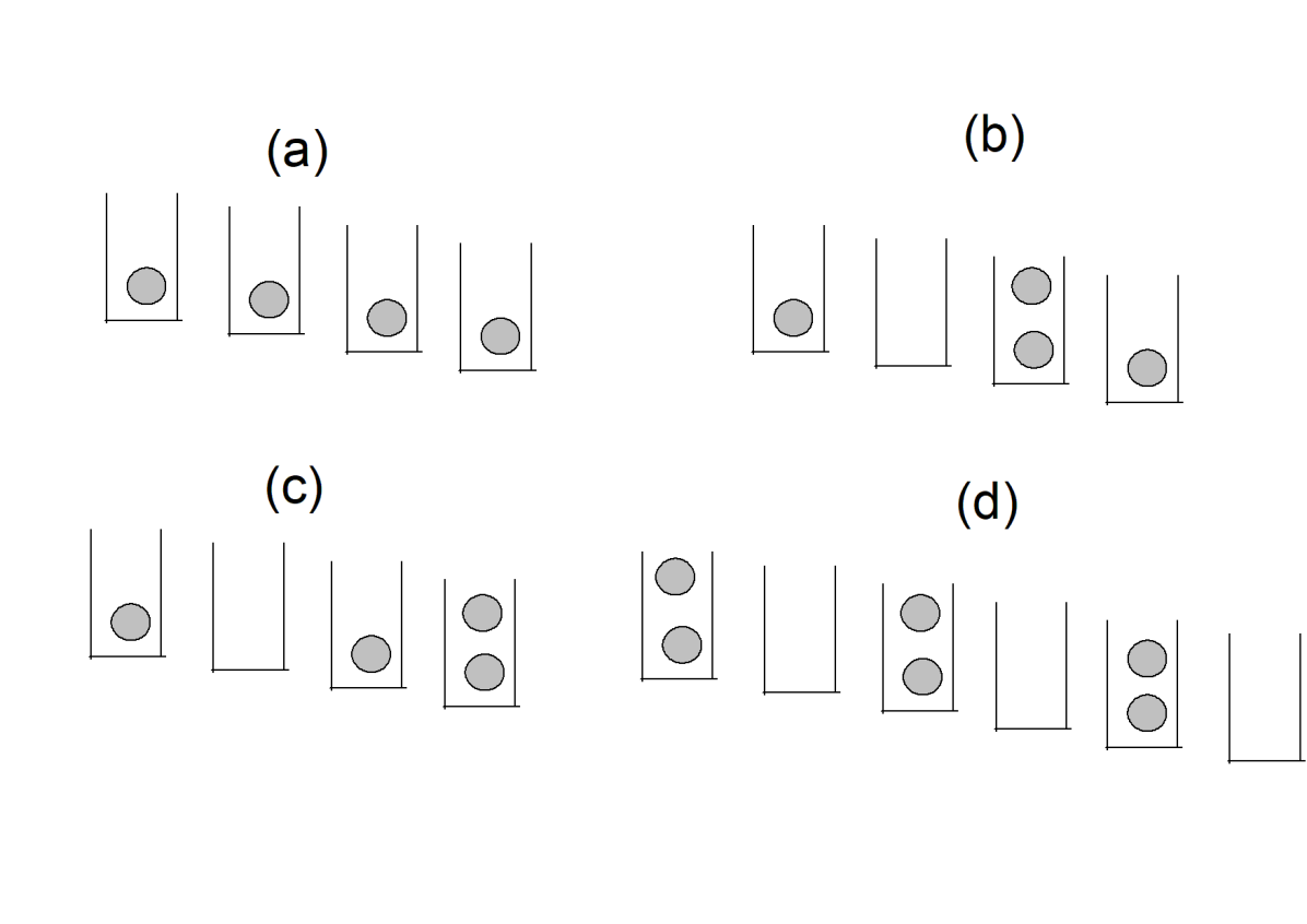
Figure 1: (a) Schematic representation of the parent Mott state with $n_{0}=1$. (b) The state with a single dipole. (c) A state with two neighboring dipoles which is equivalent to a single dipole of length two and is not a part of the low energy subspace. (d) A state with maximal number of dipoles which is also a part of the low-energy subspace.

In the presence of a tilt, the Hamiltonian of ultracold bosons in a 1D optical lattice is given by

$$H_{b} = -w\sum_{\langle jj^{\prime}\rangle}(b_{j}^{\dagger}b_{j^{\prime}}+{\rm h.c.})-\mu\sum_{j}\hat{n}_{j}+\frac{U}{2}\sum_{j}\hat{n}_{j}(\hat{n}_{j}-1)-{\mathcal{E}}\sum_{j}j\hat{n}_{j}$$ (2)

where $b_{j}$ denotes the boson annihilation operator at site $j$, $\hat{n}_{j}=b_{j}^{\dagger}b_{j}$ is the boson number operator, $w$ is their nearest-neighbor hopping amplitude, $U$ is the amplitude of the on-site interaction between the bosons, and $\mu$ denotes their chemical potential. In Eq. 2, $\langle jj^{\prime}\rangle$ indicates that $j$ and $j^{\prime}$ are nearest neighbors, and ${\mathcal{E}}$ denotes amplitude of the applied electric field in units of energy. In absence of the field, the bosons are in the in Mott state so that $\mu,U\gg w$; moreover in what follows, we shall address the physics of the system for $U,{\mathcal{E}}\gg w,|U-{\mathcal{E}}|$.

Before embarking on the description of the ground state of this model, it is useful to think about the limit $U=0$. In this case the model represents Wannier-Stark ladder for the bosons. The single-particle Schrodinger equation for such non-interacting bosons is given by (with energies $\epsilon=E+\mu$)

$$\epsilon\psi_{j} = -{\mathcal{E}}j\psi_{j}-w\left[\psi_{j-1}+\psi(j+1)\right]$$ (3)

The solution to this problem is well-known wsref . The energy of the bosons are given by $\epsilon_{m}={\mathcal{E}}m$ where $m$ denotes integers ranging from $-\infty$ to $\infty$. Note that the energy is not bounded from below and this arises from the fact that the potential is also not bounded on an infinite lattice. The eigenfunctions of the bosons are given by

$$\psi_{m}(j,t)=J_{j-m}(2w/{\mathcal{E}})\exp[-i{\mathcal{E}}mt/\hbar],$$ (4)

where $J_{n}(x)$ denotes the Bessel function. Note that the wavefunction returns to its original value at regular time intervals $t_{0}=2\pi\hbar/\mathcal{E}$ which indicates Bloch oscillations. The bosons are strongly localized to their respective site for $w\ll{\mathcal{E}}$. This behavior can also be understood from the fact that $J_{j-m}(x)$ has appreciable weight at $j=m$ for $x\ll 1$ leading to more than exponentially localized wavefunctions subir2 . This behavior is in contrast to the classical expectation where an electric field shall accelerate the bosons to the end of the chain causing an electric breakdown. This feature shall be a key component in constructing the effective theory in the limit ${\mathcal{E}}\gg w$. Such a breakdown can happen in realistic quantum systems due to electric field assisted tunneling to higher single particle bands; however for ultracold bosons, such bands are well separated in energy from the lowest bands. This leads to a tunneling time which is larger than the typical system lifetime and allows us to ignore such electric breakdown. In the absence of such breakdown, the system remains in the metastable parent state $|\psi(t=0)\rangle$. Thus the strategy adapted in Ref. subir2, for finding out the equilibrium phase of the tilted bosons was to start from the metastable parent Mott state and find out the manifold of states whose energies are close to the parent Mott state in the regime ${\mathcal{E}},U\gg w,|{\mathcal{E}}-U|$.

To understand the nature of the effective theory of the interacting bosons, we therefore start from the parent Mott state (the Mott ground state in the absence of the electric field) with $n_{0}$ bosons on every lattice site (see Fig. 1(a)) and ask how the electric field may destabilize such a bosonic system. A possibility is that this can be achieved by addition of an extra particle or hole in over the parent Mott state. The energy cost of adding a particle to the Mott state is $E_{p}=U(n_{0}+1)-\mu$ while that for a hole is $E_{h}=\mu-Un_{0}$. Note that $E_{p},E_{h}>0$ as long as the system is in the Mott ground state. However, once added, the particle[hole] sees the electric field and is thus described by an effective Hamiltonian which is identical to Eq. 3 with $\mu=0$ and $w\to w(n_{0}+1)[wn_{0}]$. They are therefore localized and can not reduce their energy via hopping (which would have been the case if ${\mathcal{E}}$ was absent). Thus such excitations are not effective in destabilizing the Mott states. This situation is therefore different from that of bosons without the tilt, where such additional particles or holes destabilize the Mott state to bring about the superfluid-insulator transition free1 ; nicolas1 .

The excited states which are part of the low-energy manifold around the parent Mott state correspond to dipole excitations where a particle hops from a lattice site to the next (Fig. 1(b)) subir2 . Such an excitation creates an additional particle on the site $j+1$ and a hole at site $j$ and thus have an energy cost

$$E_{\rm dipole} = E(n_{0}+1)+E(n_{0}-1)-2E(n_{0})-{\mathcal{E}}=U-{\mathcal{E}}$$ (5)

A state with one or multiple dipoles thus become a part of the low energy manifold for $U\simeq{\mathcal{E}}$. These states are schematically represented in Fig. 1(d). These dipoles live on the link $\ell$ between two adjacent lattice site $j$ and $j+1$. Identifying the parent Mott state as the dipole vacuum, the operators describing the creation of such dipoles can be written in terms of the boson operators as

$$d_{\ell}^{\dagger}|{\rm vac}\rangle = \frac{1}{\sqrt{n_{0}(n_{0}+1)}}b_{j}b_{j+1}^{\dagger}|{\rm Mott}\rangle$$ (6)

We note the following properties of the dipoles. First, there can be at most one dipole on any given link. This is seen by noting that creating another dipole on the same link cost an energy $E_{2}=4U-2{\mathcal{E}}$ (for $n_{0}>1$). Thus a state with two dipoles on the same link is not a part of the low energy manifold. Second, two dipoles on adjacent links cost an energy $U-2{\mathcal{E}}$ (Fig. 1(c)) (this is equivalent to a length two dipoles where a boson hops two sites as shown in Fig. 1(c)) and thus such states are also not a part of this manifold. In fact it can be shown that all longer length dipoles do not play a role subir2 . This leads to an effective dipole Hamiltonian supplemented by the constraints

$$H_{d} = -w^{\prime}\sum_{\ell}(d_{\ell}+d_{\ell}^{\dagger})+\lambda\sum_{\ell}\hat{n}_{\ell},\quad\hat{n}_{\ell}\leq 1,\quad\hat{n}_{\ell}\hat{n}_{\ell+1}=0\$$ (7)

where $\hat{n}_{\ell}=d_{\ell}^{\dagger}d_{\ell}$, $\lambda=U-{\mathcal{E}}$ and $w^{\prime}=w\sqrt{n_{0}(n_{0}+1)}$. We note that the model does not conserve dipole numbers since spontaneous hopping of bosons leads to formation/annihilation of dipoles. Moreover, the model is non-integrable due to the presence of the second constraint. The number of states in the Hilbert space of this Hamiltonian does not scale as $2^{L}$ (as that of hardcore bosons or spins); it can be shown that they scale as $\varphi^{L}$ for large $L$ where $\varphi=(1+\sqrt{5})/2$ is the golden ratio. It was shown that it is possible to write down a recursion relation for the Hilbert space dimension, ${\mathcal{N}}_{L}$, of the constrained dipole system with periodic boundary condition: ${\mathcal{N}}_{L}={\mathcal{N}}_{L-1}+{\mathcal{N}}_{L-2}$. This relates ${\mathcal{N}}_{L}$ to Fibonacci numbers $F_{L}$ for integer $L$: $N_{L}=F_{L}$ ryddyn1 .

It is easy to see that $H_{d}$ admits a representation in terms of spin-half Pauli matrices due to the constraint $\hat{n}_{\ell}\leq 1$. Indeed the mapping

$$\sigma_{\ell}^{z} = 2\hat{n}_{\ell}-1,\quad\sigma_{\ell}^{x}=(d_{\ell}+d_{\ell}^{\dagger}),\quad\sigma_{\ell}^{y}=i(d_{\ell}-d_{\ell}^{\dagger})$$ (8)

leads to the spin Hamiltonian pekker1 ; scarlit2 (up to an irrelevant constant)

$$H_{s} = \sum_{\ell}(-w^{\prime}\tilde{\sigma}_{\ell}^{x}+\lambda\sigma_{\ell}^{z}/2),\quad\tilde{\sigma}_{\ell}^{a}=P_{\ell-1}\sigma_{\ell}^{a}P_{\ell+1},\quad P_{\ell}=(1-\sigma_{\ell}^{z})/2$$ (9)

Here we have implemented the constraint $\hat{n}_{\ell}\hat{n}_{\ell+1}=0$ by using a local projection operator $P_{\ell}$ and it is understood that $H_{\rm spin}$ operates in the constrained Hilbert space where one can not have two up spins on the neighboring link. The projection operator $P_{\ell}$ ensures that this constraint is obeyed by $H_{s}$. We note here that the model, at $\lambda=0$, has been dubbed as the $PXP$ model scarlitrev ; scarlit1 ; scarlit2 ; scarlit3 ; scarlit4 ; scarlit5 .

Next, we note that addition of longer-range density-density interaction to $H_{d}$, leads to the Hamiltonian fendley1

$$H^{\prime}_{d} = H_{d}+V\sum_{\ell}\hat{n}_{\ell}\hat{n}_{\ell+2}$$ (10)

We shall not discuss the details of the phases or the dynamics of this model here but refer the readers to Refs. fendley1, ; subir2a, ; subir3, ; ghosh1, for details. The model displays a rich phase diagram and supports non-Ising quantum phase transition. Moreover, this also serves the low-energy effective model for the Rydberg atoms discussed in the last section in certain limit; we shall detail this point towards the end of this section.

The ground phase diagram of $H_{d}$ can be understood in a straightforward manner. For $\lambda\gg w^{\prime}$($U\gg{\mathcal{E}}+w^{\prime}$), the dipole excitations are energetically costly and the ground state is the dipole vacuum $|{\rm vac}\rangle$ (the parent Mott state $|{\rm Mott}\rangle$). In contrast, for $|\lambda|\gg 0$ with $\lambda<0$ (${\mathcal{E}}\gg U+w^{\prime}$), the ground state is clearly a state with maximal number of dipoles. However, due to the constraint, there are two such maximal dipole states. The first consists of dipoles are formed on the even links of the 1D lattice while the second where they are formed on the odd links. These states, for a chain of length $2L$ whose links are labeled from $0$ to $2L-1$, are (see Fig. 1(d))

$$|{\mathbb{Z}}_{2}\rangle = d_{0}^{\dagger}d_{2}^{\dagger}...d_{2L-2}^{\dagger}|{\rm vac}\rangle,\quad|{\bar{\mathbb{Z}}_{2}}\rangle=d_{1}^{\dagger}d_{3}^{\dagger}...d_{2L-1}^{\dagger}|{\rm vac}\rangle,$$ (11)

The ground state chooses one of the two states and hence breaks $Z_{2}$ symmetry. This implies that it must be separated from the dipole vacuum ground state by a transition; this quantum phase transition belongs to the Ising universality class and occurs at subir2

$${\mathcal{E}}_{c}=U+1.31\sqrt{n_{0}(n_{0}+1)}w$$ (12)

Such a transition can be understood to be the result of competition between the dipole number fluctuation arising from the first term in Eq. 7 and the effect of the electric field in the second term which makes such fluctuation energetically costly. A rough estimate of ${\mathcal{E}}_{c}$ can also be obtained from a variational wavefunction approach. The ordered state which breaks the $Z_{2}$ symmetry is characterized by an Ising order parameter. In the dipole language this order parameter can be written as

$$O = \frac{1}{2L}\sum_{\ell=0}^{2L-1}(-1)^{\ell}\hat{n}_{\ell}$$ (13)

which is the dipole density at $k=\pi$ signifying the broken translational symmetry of the ground state.

The presence of such a translational symmetry broken state was directly verified in the experiment carried out in Ref. bref2, using the fluorescence imaging technique discussed earlier. The experiment started with a Mott state having $n_{0}=1$ bosons per lattice site and generated a tilt using a linearly varying Zeeman field. Thus the parent Mott state correspond to an odd number of bosons per site and provided bright patterns in an imaging measurement. In contrast, the maximal dipole state, which constitutes an even number of states per site would provide a dark image. It was found that an increase of the strength of the magnetic field providing the tilt indeed led to a dark pattern; moreover, one could coherently interpolate between such bright and dark imaging patterns by tuning the strength of the magnetic field. This constituted the realization of the symmetry broken Mott state for ultracold bosons in an optical lattice.

Before ending this section, we briefly comment on the Rydberg atom experiments and the relation of the Hamiltonian of such Rydberg atoms with the model developed here. The low-energy effective Hamiltonian of these atoms describes the physics of the system for times which is smaller compared to typical decay scales of Rydberg excited atoms. The Hamiltonian involves two states $|g\rangle$ and $|r\rangle$. Defining $\tau_{\alpha}$ ($\alpha=x,y,z$) to be standard Pauli matrices in the space of these two states, one can write

$$H_{\rm Ryd} = -\sum_{j}(\Omega\tau_{j}^{x}+\Delta\tau_{j}^{z})+\sum_{jj^{\prime}}V_{jj^{\prime}}\hat{n}^{\prime}_{j}\hat{n}^{\prime}_{j^{\prime}}$$ (14)

where $\Delta$ and $\Omega$ has been defined in Sec. II, $V_{jj^{\prime}}$ is the dipolar interaction between two Rydberg excited atoms. Here $\hat{n}^{\prime}_{j}=(1+\tau_{j}^{z})/2$ denotes the number operator for Rydberg excitations. We note that for $V_{j,j+1}\gg\Omega,|\Delta|$ and $V_{j,j+n}\ll\Omega,|\Delta|$ for $n>2$, Eq. 14 reduces to Eq. 10 with $\Omega\to-w\sqrt{n_{0}(n_{0}+1)}$, $\Delta\to\lambda$ and $V_{j,j+2}\to V$. Moreover if $V\ll\Omega,|\Delta|$, Eq. 14 reduces to Eq. 7 (and hence to Eq. 9). It is therefore expected that the ground state phase diagram of Rydberg atoms would also reflect translational symmetry broken states for $\Delta<0$ and $|\Delta|\gg\Omega$.

In experiments carried out in Ref. gr1, , $\Delta$ could be tuned to large negative values to achieve the translational symmetry broken states. Such states had a period $2$ when $V_{j,j+1}\gg\Omega,|\Delta|$ and $V_{j,j+n}\ll\Omega,|\Delta|$ for $n>1$, in accordance with the prediction of the dipole model. In addition, it was possible to tune the strength of the Rydberg interaction such that $V_{j,j+1},V_{j,j+2}\gg\Omega,|\Delta|$ and $V_{j,j+n}\ll\Omega,|\Delta|$ for $n>2$. In this case, the ground state broke $Z_{3}$ symmetry and led to a period $3$ density-wave in accordance with that found in Ref. fendley1, by analyzing the Hamiltonian given in Eq. 10.

IV Non-equilibrium dynamics

In this section, we shall discuss the non-equilibrium dynamics of the tilted bosons in the presence of an optical lattice. The quench and the ramp dynamics of the bosons shall be discussed in Sec. IV.1 while the periodic dynamics will be addressed in Sec. IV.2.

IV.1 Quench and ramp protocols

It is well-known that ultracold atoms provide a perfect platform for studying non-equilibrium dynamics of closed quantum systems rmpks ; dziar1 ; adutta1 ; brefrev ; bookchap1 ; bookchap2 . One of the simplest protocol for such dynamics is the quench, where a parameter in the Hamiltonian of the system is changed suddenly. Consequently, the state of the system does not have time to react. The old ground state of the system (or any initial state the system might be in when the quench is performed) evolves according to the new Hamiltonian. Since the old state is no longer an eigenstate of the new Hamiltonian, it displays non-trivial dynamics. For non-integrable systems, such dynamics is expected to be lead to a thermal steady state at long times. This follows from the eigenstate thermalization hypothesis (ETH) ethref1 ; ethref2 ; ethref3 ; ethrev which predicts eventual thermalization of a typical many-body state under unitary dynamics. At short times, the system is expected to display transient oscillations.

For the tilted boson system, such oscillations were studied in Ref. ks1, . The bosons were initially assumed to a state of dipole vacuum $|0\rangle$. At $t=0$, the electric field ${\mathcal{E}}$ is changed from its initial value ${\mathcal{E}}_{i}<U$ to its final value ${\mathcal{E}}_{f}$. The state of the system at time $t$ can then be described by

$$|\psi(t)\rangle = \sum_{n}c_{n}e^{-iE_{n}t/\hbar}|n\rangle,\quad H({\mathcal{E}}_{f})|n\rangle=E_{n}|n\rangle,\quad c_{n}=\langle n|0\rangle$$ (15)

Under such evolution, the dipole order parameter given by Eq. 13 oscillates as

$$O(t) = \sum_{m,n}c_{m}c_{n}O_{mn}\cos\omega_{mn}t,\quad O_{mn}=\langle m|O|n\rangle,\quad\omega_{mn}=(E_{m}-E_{n})/\hbar$$ (16)

where we have used the fact that $c_{m}$ could be chosen to be real. A numerical evaluation of $O(t)$, carried out in Ref. ks1, (left panel of Fig. 2), showed that the transient oscillations have maximal amplitude when ${\mathcal{E}}_{f}=U$ near the critical point; they are tiny deep inside both the maximal dipole and dipole vacuum phases as shown in the left panel of Fig. 2. Thus transition can act as a qualitative marker for change in state of the system.

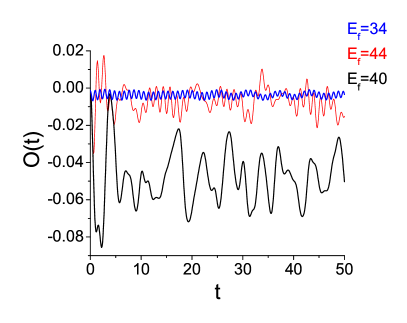
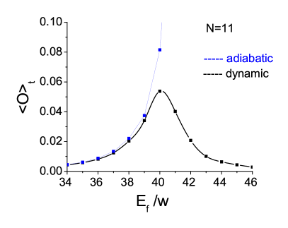
Figure 2: Left panel: Plot of $O(t)$ as a function of time for several representative values of ${\mathcal{E}}_{f}/w$. For all plots $U/w=40$ and initial state is the dipole vacuum ground state $|0\rangle$. Right panel: Plot of ${\bar{O}}\equiv\langle O\rangle_{t}$ as a function of ${\mathcal{E}}_{f}/w$ showing a peak near the critical point. In the figs $N$ represents the chain length in units of lattice spacing. This figure is adapted from Ref. ks1, .

To understand why the amplitude peaks around $U={\mathcal{E}}_{f}$, we focus on the time averaged value of these oscillations

$$\bar{O} = \lim_{T\to\infty}\frac{1}{T}\int_{0}^{T}O(t)=\sum_{m}c_{m}^{2}O_{mm}.$$ (17)

The amplitude of these oscillations is maximal when the product of overlap $c_{m}$ and order parameter expectation $O_{mm}$ is large. When ${\mathcal{E}}_{f}$ is deep inside the dipole vacuum, $c_{m}\sim 1$ when $m$ correspond to the old ground state. However, $O_{mm}\to 0$ for this state leading to a small $\bar{O}$. In contrast, when ${\mathcal{E}}_{f}$ corresponds to deep inside the maximal dipole ground state, $O_{mm}$ is large for the new ground state; however, $c_{m}\sim 0$ for this ground state leading, once again, to a small ${\bar{O}}$. In between, near the critical point, ${\bar{O}}$ could be large since both $c_{m}$ and $O_{mm}$ can be non-zero for several $m$. This leads to a peak of ${\bar{O}}$ near the critical point as shown in the right panel of Fig. 2.

More recently, the quench dynamics of Rydberg atoms has been studied experimentally starting from the $|{\mathbb{Z}}_{2}\rangle$ state gr1 . It was found that the evolution of such a state, following a quench of the parameter $\Delta\to 0$, displays long-lived coherent oscillations. Since the system is non-integrable, ETH predicts that such dynamics will lead to an eventual thermal steady state; however, such a steady state was not observed in experiments for dynamics starting from $|{\mathbb{Z}}_{2}\rangle$. In contrast, dynamics starting from the all spin-down state ($|0\rangle$ or the dipole vacuum state) showed expected, ETH predicted, thermalization. This phenomenon therefore constituted a weak (initial-state dependent) violation of ETH in such finite-sized chains.

The theoretical explanation of this phenomenon followed soon scarlitrev ; scarlit1 ; scarlit2 ; scarlit3 ; scarlit4 ; scarlit5 . The details of this has been summarized in Ref. scarlitrev, and references therein. It was found at $\Delta=0$, or in the $PXP$ limit, the eigenspectrum of $H_{s}$ (or equivalently $H_{\rm Ryd}$ for large $V_{i,i+1}$) supports a special class of eigenstates called quantum scars scarlitrev ; scarlit1 ; scarlit2 ; scarlit3 ; scarlit4 ; scarlit5 ; scarothers1 ; scarothers2 ; scarothers3 ; scarothers4 . These states have finite energy density but anomalously low half-chain entanglement entropy scarlitrev . Being anomalous, they have very little overlap with the thermal band of mid-spectrum eigenstates. Consequently, they form an almost closed subspace. It was also found that they have a strong overlap with the $|{\mathbb{Z}}_{2}\rangle$ state; thus dynamics starting from the $|{\mathbb{Z}}_{2}\rangle$ state is almost confined within the closed subspace formed by the scars leading to coherent long-lived oscillations. This does not happen for dynamics starting from the $|0\rangle$ state since it has very little overlap with the scar states. Further details of this phenomenon and properties of quantum scars is summarized in Ref. scarlitrev, .

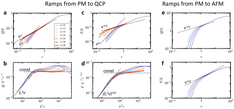
Figure 3: Plots showing behavior of (a) residual energy $Q$ as a function of $v=\tau^{-1}$ (b) $Q/(Lv)$ as a function of $v$ (c) overlap $F$ as a function of $L^{2}v$ and (d) $F/(L\sqrt{v})$ as a function of $L^{2}v$ for quench from the dipole vacuum or paramagnetic ground state(PM) to the quantum critical point (QCP). In the plot, all quantities are dimensionless, $U/w=40$, and the lattice spacing $a$ has been set to unity. For ramp from the PM to the maximal dipole or antiferromagnetic (AFM) state, the behavior of $Q$ and $F$ are shown as a function of $v$ in panels (e) and (f) respectively. This figure is adapted from Ref. pekker1, .

Next, we discuss the ramp dynamics of such a system addressed in Ref. pekker1, . In this case, one ramps the electric field via a linear protocol from its initial value ${\mathcal{E}}_{i}$ at $t=0$ to a final value ${\mathcal{E}}_{f}$ at $t=\tau$ with a rate $\tau^{-1}$: ${\mathcal{E}}(t)={\mathcal{E}}_{i}+({\mathcal{E}}_{f}-{\mathcal{E}}_{i})t/\tau$. The values of ${\mathcal{E}}_{f}$ and ${\mathcal{E}}_{i}$ are so chosen so that the system starts from the dipole vacuum state (ground state for ${\mathcal{E}}={\mathcal{E}}_{i}<U$) and reaches the critical point at ${\mathcal{E}}={\mathcal{E}}_{f}={\mathcal{E}}_{c}$. It is well known that such a passage to the critical point leads to excitation production; the density of these excitations, for slow ramp rates, scale with $\tau$ according to the Kibble-Zurek (KZ) scaling law $n_{\rm ex}\sim\tau^{-\nu d/(z\nu+1)}$, were $\nu$ and $z$ are the correlation length and dynamical critical exponents and $d$ is the spatial dimension of the system rmpks ; dziar1 ; adutta1 ; bookchap1 ; bookchap2 ; kibble1 ; zureck1 ; anatoli1 ; ks2 ; ks3 ; anatoli2 ; sondhi1 . However such scaling laws are strictly appropriate when the system size is large. For finite-sized systems such as the Rydberg chain, the system size $L$ provides a length scale which restrict the applicability of the scaling laws.

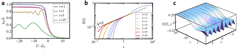
Figure 4: Plots of (a) dipole density $n_{d}$ as a function of the ramp amplitude $U-{\mathcal{E}}_{f}$ for several $v=\tau^{-1}$, (b) excitation density $D$ as a function of $v$ when ${\mathcal{E}}_{f}={\mathcal{E}}_{c}$, and (c) $C_{ii+\ell}$ as a function of $\ell$ and $v$. For all plots $U/w=40$ and the lattice spacing $a$ has been set to unity. This figure is adapted from Ref. pekker1, .

To understand why the presence of a finite-system size changes things, let us consider that the length scale $L$ leads to a energy scale $\epsilon_{0}(L)$. When the ramp rate $\tau^{-1}\leq\epsilon_{0}(L)/\hbar$, the system does not see the critical point; instead the dynamics is similar to a two-level system (the two states correspond to the instantaneous ground and first excited states near the transition where excitations are formed) with avoided level crossing, where the minimum gap is ${\rm O}(\epsilon_{0}(L))$. In this case, the excitation density scales as $n_{\rm ex}\sim\tau^{-2}$ and is independent of the critical exponents; this is known as Landau-Zenner (LZ) scaling anatoli3 . Also, when $\tau^{-1}$ is large, i.e. for fast drives, $n_{\rm ex}$ saturates and KZ scaling is not obeyed. In between, there is a finite window of drive rates for which one finds KZ scaling law. This behavior can be summed up by noting that for finite-sized system, the scaling of excitation density is described by

$$n_{\rm ex} = N^{d}\tau^{-\nu d/(z\nu+1)}f(N^{1/\nu+z}\tau^{-1}),$$ (18)

where $N=L/a$, $a$ is the lattice spacing, and the scaling function $f(x)$ satisfies $f(x)=x^{2-\nu d/(z\nu+1)}$ for $x\ll 1$ and $f(x)=1$ for $x\gg 1$. Note that $n_{\rm ex}$ crosses over from LZ to KZ scaling regime with decreasing $\tau$ around $x\simeq 1$ $\tau\sim N^{2-\nu d/(z\nu+1)}$.

The dynamics of dipole chain for such ramps have been numerically studied using exact diagonalization (ED) and time dependent matrix product states (tMPS) methods. For ED, the analysis involves finding the instantaneous eigenvalues and eigenvectors of the driven chain at $t=t_{f}=\tau$; $H[t=\tau]|n\rangle=\epsilon_{n}|n\rangle$. One can then expand the time dependent state $|\psi(t)\rangle=\sum_{n}c_{n}(t)|n\rangle$, where $c_{n}(t)=\langle n|\psi(t)\rangle$. The Schrodinger equation for the driven system can thus be written as coupled differential equations for the coefficients $c_{n}(t)$ given by

$$i\frac{dc_{n}(t)}{dt} = \epsilon_{n}c_{n}(t)+\sum_{m}\lambda_{mn}(t)c_{m}(t),\quad c_{n}(0)=\langle n|\psi(0)\rangle,\quad\lambda_{mn}(t)=(E_{f}-E_{i})(t/\tau-1)\langle m|\sum_{j}\hat{n}_{j}|n\rangle$$ (19)

These equations need to be solved numerically to obtain $|\psi(t)\rangle$. Having obtained $|\psi(t)\rangle$, one may compute several quantities such as residual energy $Q$, log fidelity $F$ (which is same as the excitation density), the dipole density $n_{d}$ and the defect density $D$ given by

$$Q = \langle\psi(\tau)|H(\tau)|\psi(\tau)\rangle-\epsilon_{0},\quad F=\ln|\langle\psi(\tau)|0\rangle\rangle|,\quad C_{\ell\ell^{\prime}}=\langle\psi(\tau)|S^{z}_{\ell}S^{z}_{\ell^{\prime}}|\psi(\tau)\rangle$$

$$n_{d} = \langle\psi(\tau)|\sum_{\ell}\hat{n}_{\ell}|\psi(\tau)\rangle,\quad D=n_{d}-\langle 0|\sum_{\ell}\hat{n}_{\ell}|0\rangle$$ (20)

where $|0\rangle$ and $\epsilon_{0}$ denotes the wavefunction and energy of the final ground state at $t=\tau$ and $S_{\ell}^{z}=2\hat{n}_{\ell}-1$.

A plot of these quantities are shown in Fig. 3 and 4 for several representative values of $L$. It was found that they exhibit KZ scaling (with exponent $\nu d/(z\nu+1)=1/2$ for $d=z=\nu=1$) within a finite window of ramp rate which depends on $L$. As $L$ increases the KZ regime holds for slower ramp rates; the crossover between the LZ and the KZ regime is shown by the sharp drops in the figures. Thus these ramped boson chains can provide experimental platform for testing KZ scaling.

Before ending this section, we would like to note that the ramp dynamics for $H^{\prime}_{d}$ (Eq. 10) has also been studied in details ghosh1 ; subir3 . Ref. ghosh1, found KZ scaling consistent with the presence of a $3$-state Potts transition in these chains. However, work of Ref. subir3, which accessed larger chain lengths, has predicted the existence of non-Ising like critical points with $z\neq 1$ (where $z$ is the dynamical critical exponent) in such chains. Since $H^{\prime}_{d}$ with large $V$ is easily reproduced in Rydberg chains, these chains can also act as platform for hosting such non-Ising quantum critical points. We shall not discuss this issue further in this article but refer the interested reader to Refs. fendley1, ; subir3, ; ghosh1, . Furthermore, the dynamics of tilted bosons in the presence of a two-rate protocol sau1 has also been discussed; it was found that such protocols may aid suppression of excitation formation in these systems uma1 .

IV.2 Periodic protocols

In this section, we shall discuss the periodically driven tilted boson chains ryddyn1 ; ryddyn2 ; ryddyn3 . For the rest of this article, we shall explicitly use the spin representation and work with $H_{s}$ (Eq. 9). The connection of the spins with the original dipoles is given by Eq. 8. The methods used shall be briefly discussed in Sec. IV.2.1 while the main results shall be presented in Sec. IV.2.2.

IV.2.1 Methods

The properties of a periodically driven system is best described in terms of its Floquet Hamiltonian $H_{F}$ which is related to the unitary time evolution operator $U$ by $U(T,0)=\exp[-iH_{F}T/\hbar]$, where $T=2\pi/\omega_{D}$ is the time period of the drive, $\omega_{D}$ is the drive frequency, and the wavefunction of the driven system at any time $t$ is related to the initial wavefunction by $|\psi(t)\rangle=U(t,0)|\psi(0)\rangle$. Thus the stroboscopic dynamics of the system at $t=nT$, where $n$ is an integer is completely controlled by its Floquet Hamiltonian flref1 ; flref2 ; asenrev

The Floquet Hamiltonian of any periodically can be computed by comparing two equivalent expressions for $U(T,0)$

$$U(T,0) = T_{t}\left\{\exp\left[-i\int_{0}^{T}dtH(t)/\hbar\right]\right\}=\exp\left[-iH_{F}T/\hbar\right]$$ (21)

For an interacting many-body system, it is usually not possible to obtain $H_{F}$ exactly. This has led to several approximation schemes for such computations asenrev . In what follows, we shall mostly use one of these schemes, namely, the floquet perturbation theory (FPT) dsen1 ; tb1 ; ghosh2 ; asenrev , to obtain the Floquet Hamiltonian for the driven dipole chain. This method involves a perturbation in drive amplitude; the term in $H(t)$ with the largest amplitude is treated exactly, while the other terms are treated using standard time-dependent perturbation theory asenrev . In contrast to the Magnus expansion technique, the drive period $T$ need not be a small parameter here; thus, the method allows us to access the intermediate drive-frequency regime which can not be accessed using Magnus expansion.

To study the properties of the periodically driven chain, we choose to vary the electric field according to the square pulse protocol such that

$$\lambda(t) = -(+)\lambda_{0}/2\quad{\rm for}\,\,t\leq(>)T/2$$ (22)

where $\lambda_{0}$ denotes the amplitude of the drive. In what follows, we shall address the regime where $\lambda_{0}\gg w$. In this regime, the drive term is the one which has the largest amplitude. Thus we write

$$H_{s}(t) = H_{s0}(t)+H_{s1},\quad H_{s0}(t)=\lambda(t)\sum_{j}\sigma_{j}^{z},\quad H_{s1}=-w\sum_{j}\tilde{\sigma}_{j}^{x}$$ (23)

and treat $H_{s0}(t)$ exactly. Noting that $H_{s0}$ is diagonal in the spin basis, we consider a complete set of states in the constrained Hilbert space which has $m$ up-spins and denotes these states as $|m\rangle$. Note that the positions of these spins (as long as they are not nearest neighbors) do not change their instantaneous energy under action of $H_{s0}$; thus each $|m\rangle$ represents a degenerate manifold of states. Using these states as basis states one finds

$$U_{0}(t,0) = e^{i\lambda_{0}t\sum_{j}\sigma_{j}^{z}/(2\hbar)}\quad{\rm for}\quad t\leq T/2$$ (24)

$$= e^{i\lambda_{0}(T-t)\sum_{j}\sigma_{j}^{z}/(2\hbar)}\quad{\rm for}\quad t\geq T/2$$

so that $\langle m|U_{0}|n\rangle\sim\delta_{mn}$. We also note that for $t=T$, $U_{0}(T,0)=I$ (where $I$ is the identity matrix); thus $H_{F}^{(0)}=0$ for this protocol. This is a consequence of the symmetric nature of the drive (Eq. 22) which leads to a vanishing average of $\lambda(t)$ over a drive cycle.

The first order perturbative correction to the evolution operator $U$ can be obtained using standard time dependent perturbation theory. This is given by

$$U_{1}(T,0) = \frac{-i}{\hbar}\int_{0}^{T}dtU_{0}^{\dagger}(t,0)H_{s1}U_{0}(t,0)$$ (25)

We note that $\tilde{\sigma}_{j}^{x}$ flips a spin on the $j^{\rm th}$ site, $\langle m|H_{s1}|n\rangle\sim\delta_{m,n\pm 1}$. Denoting a state $|m+(-)\uparrow_{j}\rangle$ to be the one with one additional (less) spin up residing at the $j^{\rm th}$ site, we can therefore write ryddyn1 ; ryddyn2 ; ryddyn3

$$U_{1}(T,0) = \sum_{m}\sum_{j}\sum_{s_{j}=\pm 1}c^{(1)}_{s_{j}}|m\rangle\langle m+s_{j}|,\quad c^{(1)}_{s}=\frac{4iw}{\lambda_{0}}e^{i\lambda_{0}Ts/(4\hbar)}\sin\lambda_{0}T/(4\hbar)$$ (26)

where $s=\pm 1$. Noting that $\tilde{\sigma}^{\pm}|m\rangle=|m\pm 1$, and using Eq. 21 we get, to first order in $w/\lambda_{0}$

$$H_{F}^{(1)} = -w\frac{\sin\gamma}{\gamma}\sum_{j}(\cos\gamma\tilde{\sigma}_{j}^{x}+\sin\gamma\tilde{\sigma}_{j}^{y}),\quad\gamma=\lambda_{0}T/(4\hbar).$$ (27)

We note that for $T\to 0$, $\gamma\to 0$, and in this limit $H_{F}^{(1)}=-w\sum_{j}\tilde{\sigma}_{j}^{x}=H_{\rm PXP}$. This is also consistent with the Magnus result for $H_{F}$ which demands that $H_{F}$ shall be average Hamiltonian given by

$$H_{F}^{\rm magnus} = \frac{1}{T}\int_{0}^{T}H(t)dt=H_{\rm PXP}$$ (28)

Also, at this order, $H_{F}^{(1)}$ represents a PXP like Hamiltonian up to a rotation and an overall renormalization by a factor $\sin\gamma/\gamma$; it was noted in Ref. ryddyn1, that this result constitutes a resummation of a class of terms in the Magnus expansion.

The higher order terms in the Floquet Hamiltonian can also be computed. This has been carried out systematically in Ref. ryddyn3, and leads to $H_{F}^{(2)}=0$ at second order. This null result for $H_{F}$ to second order owes it existence to the fact that there exists an operator $C=\prod_{j}\sigma_{j}^{z}$ which satisfies $CU(T,0)C=U^{-1}(T,0)$ leading to $\{H_{F},C\}=0$. As shown in Refs. scarlitrev, ; ryddyn1, , such anti-commutation only allows for odd orders in the Floquet Hamiltonian. At third order, a straightforward but tedious calculation ryddyn3

$$H_{F}^{(3)} = -\alpha_{0}\sum_{j}\left[\left(\tilde{\sigma}_{j+1}^{+}\sigma_{j-1}^{+}+\tilde{\sigma}_{j-1}^{+}\tilde{\sigma}_{j+1}^{+}\right)\tilde{\sigma}_{j}^{-}-6\tilde{\sigma}_{j}^{+}\right]+{\rm h.c.},$$

$$\alpha_{0} = \left[e^{3i\lambda_{0}T/(2\hbar)}+3e^{i\lambda_{0}T/(2\hbar)}(1+i\lambda_{0}T/\hbar)+2(1-3e^{i\lambda_{0}T/\hbar})\right]\frac{\hbar w^{3}e^{-i\lambda_{0}T/\hbar}}{3i\lambda_{0}^{3}T}.$$ (29)

The first term in $H_{F}^{(3)}$ involves three spin on neighboring sites. We note that the form of this term, i,e., the order in which the $\tilde{\sigma}^{\pm}$ operators appear, is dictated by the presence of the constraint; the order of appearance ensures that two neighboring sites can never have two up-spins. The second term of the Floquet Hamiltonian provides a shift to $H_{F}^{(1)}$ and renormalize its coefficients. In what follows, we shall use this perturbative Floquet Hamiltonian to understand the numerical results.

The numerical approach to this problem, carried out in Ref. ryddyn1, ; ryddyn3, used exact diagonalization(ED). The first step in this direction involves numerical diagonalizaton of $H[\pm\lambda_{0}]$. We denote the corresponding energy eigenvalues and eigenvectors by

$$H[\pm\lambda_{0}]|p_{\pm}\rangle = \epsilon_{p}^{\pm}|p_{\pm}\rangle$$ (30)

In terms of this, the evolution operator can be written as

$$U(T,0) = e^{-iH[\lambda_{0}]T/(2\hbar)}e^{-iH[-\lambda_{0}]T/(2\hbar)}=\sum_{p,q}c_{pq}^{-+}e^{-i(\epsilon_{p}^{-}+\epsilon_{q}^{+})T/(2\hbar)}|p^{-}\rangle\langle q^{+}|,\quad c_{pq}^{-+}=\langle p^{-}|q^{+}\rangle$$ (31)

Thus one has a finite-dimensional matrix (for finite sized $L$) which can then be diaonalized. Since $U$ is an unitary operator. its eigenvalues are unimodular. Thus one can express it in term of its eigenspectra as

$$U(T,0) = \sum_{\alpha}e^{-i\epsilon_{\alpha}^{F}T/\hbar}|\alpha\rangle\langle\alpha|,\quad H_{F}|\alpha\rangle=\epsilon_{\alpha}^{F}|\alpha\rangle$$ (32)

where $|\alpha\rangle$ are the eigenfunctions of $U(T,0)$, $\epsilon_{\alpha}^{F}$ are the eigenvalues of the corresponding Floquet Hamiltonian, and the last equation follows from Eq. 21. This procedure thus allows access to the exact Floquet quasienergies and eigenfunctions for finite-sized systems. The stroboscopic evolution, at $t=nT$ ( where $n$ is an integer), for any operator ${\mathcal{O}}$, can thus be computed as ryddyn1

$${\mathcal{O}}_{n} = \langle\psi(0)|(U^{\dagger}(T,0))^{n}{\mathcal{O}}U^{n}(T,0)|\psi(0)\rangle=\sum_{\alpha,\beta}c_{\beta}^{\ast}c_{\alpha}e^{-i(\epsilon_{\alpha}^{F}-\epsilon_{\beta}^{F})T/\hbar}\langle\beta|{\mathcal{O}}|\alpha\rangle$$ (33)

where $|\psi(0)\rangle$ is the initial state and $c_{\alpha}=\langle\psi(0)|\alpha\rangle$.

In what follows, we shall also be computing the half-chain entanglement entropy of the Floquet eigenstates. The procedure for this is as follows. First, corresponding to any eigenstate $|\psi_{n}\rangle$, we construct a density matrix $\rho_{n}=|\psi_{n}\rangle\langle\psi_{n}|$ which is defined on the full chain with periodic boundary condition. Next we divide the chain into two equal halves, $A$ and $B$, with open boundary condition and trace out the contribution of states residing in $B$. Thus each matrix element of the reduced density matrix $\rho^{A}_{n}$ after tracing out $B$ can be written as ryddyn1

$$\langle\rho_{n}^{A}\rangle_{\alpha\beta} = \sum_{\mu\in B=1}^{{\mathcal{N}}_{B}}\langle\alpha;\mu|\rho_{n}|\beta;\mu\rangle$$ (34)

where ${\mathcal{N}}_{B}$ denotes the Hilbert space dimension corresponding to states residing in $B$ with open boundary condition and the states $|\alpha\rangle$ and $|\beta\rangle$ have weights in region $A$ ryddyn1 . While carrying out this procedure, one has to be careful in excluding states where the right end of $A$ and the left end of $B$ both has spin-up (or dipoles) since these states were not part of the Hilbert space of the full chain owing to the constraint. The half-chain entanglement $S_{L/2}^{(n)}$ can then be obtained numerically using

$$S^{(n)}_{L/2} = -\sum_{j=1}^{{\mathcal{N}}_{A}}q_{j}\ln q_{j}$$ (35)

where $q_{j}$ denotes the eigenvalues of $\rho_{n}^{A}$ obtained via numerical diagonalization. We shall use $S^{(n)}_{L/2}$ to distinguish between states with volume- and area-law entanglement entropies in the rest of this article.

IV.2.2 Results

To study the physics of the driven dipole chain, we concentrate on half-chain entanglement $S_{L/2}$ (Eq. 35) of the Floquet eigenstates and the density-density correlator $\langle O_{j2}\rangle=\langle\psi(nT)|\hat{n}_{j}\hat{n}_{j+2}|\psi(nT)\rangle$, where $\hat{n}_{j}=(1+\sigma_{j}^{z})/2$. In what follows, we shall discuss the property of the stroboscopic evolution of $\langle O_{22}\rangle$ (i.e. choosing $j=2$) starting from either the $|{\mathbb{Z}}_{2}\rangle$ (antiferromagnetic state with up-spins on even sites) or the $|0\rangle$ (ferromagnetic all spin-down state) state. The evolution of $\langle O_{jj+2}\rangle$ for other values of $j$ is identical as long as $j$ is chosen to be even ryddyn1 ; ryddyn2 ; ryddyn3

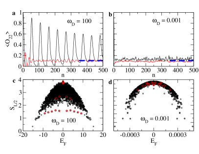
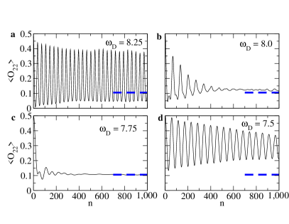
Figure 5: Left Panel: Plot of $\langle O_{22}\rangle$ as a function of number of drive cycles $n$ for (a) $\hbar\omega_{D}=100$ and (b) $\hbar\omega_{D}=0.01$. The red lines indicates dynamics starting from the state $|0\rangle$ while the black lines indicate $|{\mathbb{Z}}_{2}\rangle$ The ETH predicted thermal steady state value of $\langle O_{22}\rangle$ is $\sim 0.11$ as shown in blue dotted line. Plots (c) and (d) shows the corresponding half-chain entanglement $S_{L/2}$. Note the presence of athermal scar states below the thermal band for $\hbar\omega_{D}=100$. Such states are absent for $\hbar\omega_{D}=0.01$. The red circles correspond to states which has high overlap with the initial $|{\mathbb{Z}}_{2}\rangle$ state. For all plots $\lambda=15$, $w=\sqrt{2}$, $\hbar$ is set to unity, and $L=18$. Right Panel: Plot of $O_{22}$ as a function of $n$ for (a) $\hbar\omega_{D}=8.25$, (b) $\hbar\omega_{D}=8$, (c) $\hbar\omega_{D}=7.75$, and (d) $\hbar\omega_{D}=7.5$. The plot for (a) and (d) shows coherent oscillation while those for (b) and (c) exhibits rapid approach to ETH predicted thermalization. All other parameters are same that in the left panel. This figure is adapted from Ref. ryddyn1, .

We first consider the dynamics starting from the $|{\mathbb{Z}}_{2}\rangle$ initial state. For this state, for $\lambda_{0}/(\hbar\omega_{D})\ll 1$, the dynamics is similar to that of quench studied in Ref. scarlitrev, . In this regime, we expect scar-induced coherent oscillations with a frequency which is determined by the energy separation between the quantum scar eigenstates. In the opposite limit, $w/(\hbar\omega_{D})\gg 1$ (where FPT and Magnus expansion both fail) it is expected that the system shall heat up due to the drive and reach the thermal steady state as predicted by ETH. This expectation is verified from the behavior of $\langle O_{22}\rangle$ shown for high and low frequencies in the plots shown at the top of the left panel in Fig. 5. The bottom plots of the left panel of Fig. 5 shows the half-chain entanglement entropies of the Floquet eiegnstates at these drive frequencies; the high frequency eigenstates clearly show the presence of athermal scars separated from the thermal band of states. No such athermal states are seen at low drive frequency; in this regime, all the states fall within the thermal band. The red dots indicates eigenstates with large overlap with the initial $|{\mathbb{Z}}_{2}\rangle$ state. These are the states which primarily drive the dynamics. At high frequency, these states are athermal and lie well outside the thermal band. Thus the dynamics exhibit coherent oscillations since it involves a small, ${\rm O}(L)$, subspace of the full Hilbert space. In contrast, at low frequency, the eigenstates having large overlap with $|{\mathbb{Z}}_{2}\rangle$ are part of the thermal band leading to thermalization.

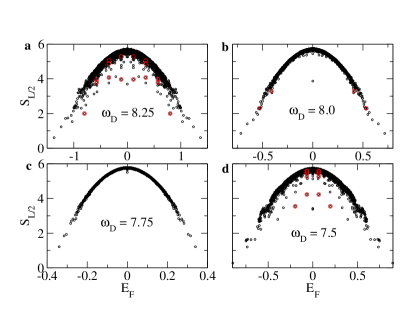
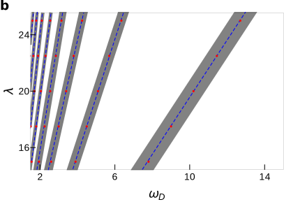
Figure 6: Left Panel: Plots of half-chain entanglement entropy $S_{L/2}$ for (a) $\hbar\omega_{D}=8.25$ (b)$\hbar\omega_{D}=8$, (c) $\hbar\omega_{D}=7.75$, and (d) $\hbar\omega_{D}=7.5$. The plots shows athermal scar states below the thermal band with low $S_{L/2}$ at $\hbar\omega_{D}=8.25$ and $\hbar\omega_{D}=7.5$ while no such states are found for $\hbar\omega_{D}=8$ and $7.75$. The red circles exhibits states which has high overlap with the initial $|{\mathbb{Z}}_{2}\rangle$. For all plots, $\lambda=15$, $w=\sqrt{2}$ and $L=18$ and we have set $\hbar=1$. Right Panel: Phase diagram in the $\lambda-\omega_{D}$ plane showing ergodic (shaded) and coherent (white) regions with reentrant crossover between them. All other parameters are same as those in the left panel. This figure is adapted from Ref. ryddyn1, .

Naively, one would expect a crossover between these two regimes at some intermediate drive frequency. In contrast, as shown, in the right panel Fig. 5, the system exhibits non-monotonic re-entrant behavior at multiple intermediate frequencies. This is most easily noted by comparing the four plots in the right panel of Fig. 5. Clearly, ETH predicted thermalization is restored around $\hbar\omega_{D}\simeq 7.75w$; however, scar induced oscillations take over at a lower drive frequency $\hbar\omega_{D}\simeq 7.5w$. The corresponding half-chain entanglement entropies, shown in the left panels of Fig. 6, indicate the presence of scars at $\hbar\omega_{D}=7.5w$ and their absence at $\hbar\omega_{D}=7.75w$. Further studies, carried out in Ref. ryddyn1, , demonstrates multiple crossovers between ETH predicted ergodic and scar-induced coherent oscillatory behaviors at intermediate frequencies leading to the phase diagram shown in the right panel of Fig. 6. The density of the ergodic regimes increases with lower frequency and they completely cover the phase diagram at low drive frequencies leading to ergodic behavior in this regime. However, at intermediate frequencies, as shown in Ref. ryddyn1, , it is possible to tune into and out of such ergodic regimes by tuning the drive frequency. This leads to the possibility of drive-frequency induced tuning of ergodicity in a driven non-integrable system.

This tunability of ergodicity can be qualitatively understood from the analytical Floquet Hamiltonian (Eqs. 27 and 29) as follows. For $\hbar\omega_{D}\gg\lambda_{0}$, $\sin\gamma\sim\gamma$ and $H_{F}^{(1)}\simeq H_{\rm PXP}$. Moreover since $w/\lambda_{0}\ll 1$, $H_{F}^{(3)}$ is negligible compared to $H_{F}^{(1)}$ in this limit. Thus the Floquet Hamiltonian is of the PXP form and supports quantum scars. For an initial state $|{\mathbb{Z}}_{2}\rangle$, the dynamics gets maximal contribution from the scar subspace leading to coherent oscillation scarlitrev . In contrast around $\gamma\simeq m\pi$ (where $m$ is a non-zero integer), $H_{F}^{(1)}\to 0$ and $H_{F}^{(3)}$ dominates. The Floquet Hamiltonian is then not of the PXP form anymore and does not support scar states with large overlap with $|{\mathbb{Z}}_{2}\rangle$. Consequently, the dynamics becomes ergodic around $\omega_{D}=\omega_{D}^{c}=\gamma_{0}/(2m\hbar)$; the width of the ergodic regime depends on the relative magnitudes of $H_{F}^{(1)}$ and $H_{F}^{(3)}$ as we move away $\omega_{D}^{c}$. Of course, this estimate of $\omega_{D}^{c}$ does not take into account the renormalization of $H_{F}^{(1)}$ from the higher order terms (such as the one from $H_{F}^{(3)})$ and is thus not exact. However since these terms are typically small in the intermediate frequency regime by a factor of at least $w^{3}/\lambda_{0}^{3}\ll 1$, this estimate turns out to be qualitatively correct.

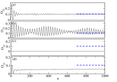
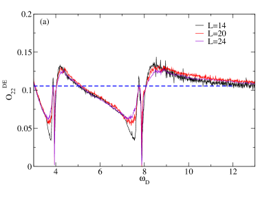
Figure 7: Left Panel: Plot of $\langle O_{22}\rangle\sim O_{22}$ as a function of $n$ for (a) $\hbar\omega_{D}=100$ (b)$\hbar\omega_{D}=8.5$, (c) $\hbar\omega_{D}=7.88$, and (d) $\hbar\omega_{D}=7.25$. For all plots, $\lambda=15$, $w=\sqrt{2}$ and $L=26$ and we have set $\hbar=1$. Right Panel: The steady state value of $\langle O_{22}\rangle\equiv O_{22}^{\rm DE}$ as a function of $\omega_{D}$ for several $L$. For all plots $\lambda=15$, $w=\sqrt{2}$ and $\hbar$ is set to unity. This figure is adapted from Ref. ryddyn3, .

Next, we consider the stroboscopic dynamics of $\langle O_{22}\rangle$ starting from the $|0\rangle$ state. We note that for $\hbar\omega_{D}/\lambda_{0}\gg 1$, the dynamics exhibits thermalization consistent with the ETH prediction as can be seen from the left panel of Fig. 5. Thus in the quench limit, scars do not play a role in the dynamics since they have negligible overlap with the $|0\rangle$ state. As the drive frequency is lowered, however, the situation changes as can be seen from left panel of Fig. 7. Around $\hbar\omega_{D}=8.5w$, we find the presence of long-time coherent oscillations while at $\hbar\omega_{D}=7.88w$, $\langle O_{22}\rangle$ remains completely frozen to its initial value. The latter behavior constitutes dynamic freezing in an otherwise ergodic non-integrable system. Finally, for $\hbar\omega_{D}=7.26w$, we find that $\langle O_{22}\rangle$ reaches a steady state value which is lower than the ETH predicted value (shown by the blue dotted line). This constitutes a qualitatively different violation of ETH since coherent scar-induced oscillatory dynamics (such as the one seen for $\hbar\omega_{D}=8.5w$) usually leads to super-thermal steady state values in contrast to the subthermal value found in the present case. The steady state behavior of $\langle O_{22}\rangle$ starting from $|0\rangle$ initial state is shown in the right panel of Fig. 7. We find that the steady state reaches its thermal value, shown by the dotted line, at large $\omega_{D}$. As the frequency is lowered, it reacher superthermal steady state value. Here the dynamics indicates coherent long-time stroboscopic oscillation. Just below $\hbar\omega_{D}<8w$, the steady state value of $\langle O_{22}\rangle$ drops and reaches zero at $\hbar\omega_{D}\simeq 7.88w$. This constitutes an example of dynamical freezing dynfr1 ; dynfr2 . This is followed by a wide range of frequency at which the steady state value remains subthermal. We also note the presence of a second freezing point at around $\hbar\omega_{D}\simeq 3.95w$. These steady state values of $O_{22}$ seem to be independent of system size within the range of $L$ accessible within ED.

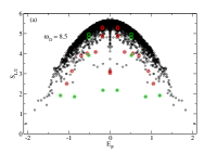
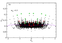
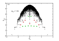
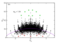
Figure 8: Leftmost Panel: Plot of $S_{L/2}$ as a function of $E_{F}$ for $\hbar\omega_{D}=8.5$. The green circles indicate states having large overlap with $|{\bar{Z}}_{2}\rangle$ while the red circles indicates those having large overlap with $|0\rangle$. For all plots, $\lambda=15$, $w=\sqrt{2}$ and $L=26$. Left-center Panel: Plot of $\langle|O_{22}|\rangle\equiv O_{22}$ for all Floquet eigenstates. The red and the green circles indicates contribution from states with large overlap with $|0\rangle$ and $|{\mathbb{Z}}_{2}\rangle$ respectively. The violet dotted line indicates the ETH prediction for $O_{22}$. Right-center and Rightmost Panels: Same as the leftmost and the left-center panels respectively but for $\hbar\omega_{D}=7.26$. This figure is adapted from Ref. ryddyn3, .

The oscillatory behavior of $O_{22}$ starting from $|0\rangle$ can be understood by observing the nature of the Floquet eigenstates as shown in the leftmost panel of Fig. 8. The plot shows the presence of a different set of athermal states (indicated by red circles) which has large overlap with the $|0\rangle$. These states are different from the scars which has large overlap with $|{\mathbb{Z}}_{2}\rangle$ shown by green circles. Thus the Floquet hamiltonian at these frequencies supports at least two separate set of scar states; this phenomenon has no analog in scars of the PXP model. Indeed, as the frequency is increased, the set of scar states which has large overlap with $|0\rangle$ merge into the continuum of thermal states leaving behind only athermal $|{\mathbb{Z}}_{2}\rangle$ scars. This brings out the central role of higher order terms in the Floquet Hamiltonian for generation of such scars. The presence of such scars lead to coherent oscillatory dynamics of $O_{22}$. Its steady state value turns out to be superthermal which can be seen from the left-center panel of Fig. 8. This is due to the fact that for most scar eigenstates that have large overlap with $|0\rangle$ (shown as red circles in the left-center panel of Fig. 8), $\langle O_{22}\rangle$ is larger than the ETH predicted thermal value.

Similar scar states with large overlap with $|0\rangle$ is shown by red circles in the right-center panel of Fig. 8 for $\hbar\omega_{D}=7.26w$. Here in contrast to the case $\hbar\omega_{D}=8.5$, the initial state $|0\rangle$ turns out to have relatively large overlap ($>0.01$) with a few scars states as shown in the figure and small overlap with a large number of thermal states. The presence of these thermal states do not allow for long time coherent oscillations. However, the steady state value of $\langle O_{22}\rangle$ is controlled by the athermal scar states since they have relatively large overlap with $|0\rangle$. It turns out that these athermal scar states have a subthermal value of $\langle O_{22}\rangle$ (as can be seen from the rightmost panel of Fig. 8). Thus $\langle O_{22}\rangle$ quickly decays to a subthermal steady state value leading to violation of ETH. We note that such a violation do not involve oscillatory dynamics and thus constitute a separate route of scar-induced ETH violation in finite boson chains which has no analogue in chains subjected to quench. ryddyn3 .

Finally, we discuss the phenomena of dynamic freezing at $\hbar\omega_{D}\simeq 7.88$ for $w=\sqrt{2}$ and $\lambda=15$. Qualitatively, the existence of such freezing is easy to understand by noting that the state $|0\rangle$ is annihilated by all non-PXP higher order terms of the Floquet Hamiltonian. This follows from the fact that such terms necessarily involves $\tilde{\sigma}_{j}^{-}$ operator which annihilates the state $|0\rangle$. Thus for drive period, where the coefficient of $H_{F}^{(1)}$ vanishes, $U(T,0)\to I$ and one encounters freezing. This argument, in conjunction with the first order perturbative Floquet Hamiltonian, suggest that the freezing would occur at frequencies for which $w_{r}=0$: $\hbar\omega_{D}=\lambda/(2n)$. This predicts a freezing frequency of $\hbar\omega_{D}=7.5$ which differs quite a bit with the exact result.

This discrepancy can be understood by noting that the first order Floquet Hamiltonian neglects the normalization of $w_{r}$ due to contribution of higher order term such as the one from $H_{F}^{(3)}$ (Eq. 29). To see this, we consider an exact analytical calculation of $H_{F}$ for $L=3$. Here the exact analytic calculation is feasible since the Hilbert space consists of just two states in the zero momentum sector; this reduces the problem to a driven two-state problem ryddyn3 . These two states are $|0\rangle=|\downarrow,\downarrow,\downarrow\rangle$ and $|1\rangle=(|\downarrow,\uparrow,\downarrow\rangle+|\uparrow,\downarrow,\downarrow\rangle+|\downarrow,\downarrow,\uparrow\rangle)/\sqrt{3}$. The Hamiltonian, the space of these two states, reads

$$H_{2}(t) = \left(\begin{array}[]{cc}0&-\sqrt{3}w\\ -\sqrt{3}w&\lambda(t)\end{array}\right)$$ (38)

For the square pulse protocol given by Eq. 22 the Floquet Hamiltonian $H^{\prime}_{F}$ corresponding to $H_{2}(t)$ can be exactly computed ryddyn3 . A straightforward calculation shows that

$$\langle 0|H^{\prime}_{F}T|1\rangle = \cos^{-1}\left[1-\frac{12w^{2}}{\Delta_{0}^{2}}\{1-\cos(\Delta_{0}T/2)\}\right],\quad\Delta_{0}=\sqrt{\lambda_{0}^{2}+12w^{2}}$$ (39)

This matrix element, which needs to be finite for the driven system to evolve, vanishes for $\Delta_{0}T=4m\pi$ (where $m$ is an integer). For $\lambda=15$ and $w=\sqrt{2}$, $\hbar\omega_{D}\simeq 7.86$ for $m=1$, and this provides a near exact match to the observed freezing frequency. Moreover, it also predicts the second freezing point at $\hbar\omega_{D}\simeq 3.93$ which correspond to $m=2$. We note that for $\lambda\gg w$, this frequency will reduce to that predicted by first order Floquet theory ($\hbar\omega_{D}=\lambda/2m$) as expected. The reason for the accuracy of the result obtained with this simplistic calculation is that the higher order multiple spin terms in $H_{F}$ do not contribute to the freezing phenomenon as discussed earlier. We note that at the freezing point the state $|0\rangle$ is disconnected from all other states in the Hilbert space of the system; this constitutes an example of (weak) fragmentation of the Hilbert space of $H_{F}$.

Before ending this section, we note that the periodic dynamics of Rydberg atoms has been studied experimentally in Ref. gr4, . The experiment used a continuous drive protocol using a damped cosine drive and starting from $|Z_{2}\rangle$; it was found the system exhibits a robust subharmonic response to the drive. It was noted that this response depended on the initial state and its relation to quantum scars in the system was discussed. However, the dynamics of the system starting from $|0\rangle$ state or that in the presence of a square pulse protocol has not been studied in this work.

V Hilbert space fragmentation: A minimal model

It has been recently been pointed out that the presence of dynamical constraints in a many-body system may lead to fragmentation of its Hilbert space into several disconnected sectors. This phenomenon, termed as Hilbert space fragmentation (HSF), provides yet another route to violation of ETH in non-integrable quantum systems fraglitrev ; fraglit1 ; fraglit2 ; fraglit3 ; fraglit4 ; fraglit5 ; fraglit6 ; fraglit7 ; fraglit8 ; bm1 . This phenomenon naturally arises in constrained systems where the presence of additional conservation laws provide the constraint fraglitrev ; fraglit1 ; fraglit2 ; fraglit3 ; fraglit4 ; fraglit5 ; fraglit6 ; fraglit7 ; fraglit8 . The resulting physics has close similarity with those of fractons fracrev1 ; fracrev2 . The realization of such constrained systems using circuit models whose Hilbert space is identical to that of a $S=1$ spin chain of length $L$ provides a neat example in this context fraglit2 . In this case, it was shown that the presence of two simultaneous $U(1)$ conserved quantities, namely $Q=\sum_{j}S_{j}^{z}$ (which is analogous to total charge in a fractonic model) and $P=\sum_{j}jS_{j}^{z}$ (dipole moment of a fractonic model), provides the necessary constraints for fragmentation. Typically, in most of the models studied, such conservation comes from the commutation $[Q,H]=[P,H]=0$ and remains valid for all states in the Hilbert space; moreover, they lead to an exponentially large number of inert zero-energy states in the Hilbert space. We note here such fragmentation may even separate states with same symmetry into different, disconnected, segments within the Hilbert space. Such fragmentation is dubbed as ”strong” if the Hilbert space is fragmented in exponentially many separate sectors; in this case, the number of states which lead to violation of ETH increases exponentially with system size fraglitrev ; fraglit3 . If this condition is not satisfied, the fragmentation is termed as weak; in this sense, scars constitutes an example of weak fragmentation of Hilbert space. A recent experiment involving Fermi-Hubbard model has observed non-ergodic behavior in a titled Fermi-Hubbard system which can possibly be attributed to such fragmemntation fragexp . In the rest of this section, we shall discuss such fragmentation in a model which was inspired by the Floquet Hamiltonian of the tilted Bose-Hubbard model; the details of HSF and its realization in other model can be found in Ref. fraglitrev, .

V.1 Model and fragmentation

The tilted Bose-Hubbard model constitutes an example of a spin-half system in a constrained Hilbert space. However, the model does not show HSF. The reason for this becomes clear when one analyzes the connectivity of the states of the model in the number basis in the PXP limit. It turns out, as noted in Ref. bm1, , that most states in the Hilbert space are connected under the action of $H_{\rm PXP}$ via the state $|0\rangle$. Thus a Hamiltonian which would annihilate the state $|0\rangle$ may lead to HSF. Taking cue from the structure of the Floquet Hamiltonian for the periodic driven tilted Bose-Hubbard model, Ref. bm1, pointed out that one such possible model involving spin-half Pauli matrices on a 1D chain is given by

$$H_{\rm fr} = w\sum_{j=1}^{L}\tilde{(}\sigma_{j-1}^{+}\tilde{\sigma}_{j+1}^{+}\tilde{\sigma}_{j}^{-}+{\rm h.c.}),$$ (40)

where $w$ is an arbitrary energy scale which shall be set to unity for the rest of this section and it is understood that $H_{\rm fr}$ acts on the constrained Hilbert where two up-spins can not be neighbors. We note that $H_{\rm fr}$ is identical to the three-spin term in the third order Floquet Hamiltonian (Eq. 29) but with its coefficient set to unity. Such a term becomes the largest term in $H_{F}$ around the point where renormalized $H_{F}^{(1)}$ (Eq. 27) vanishes. We note that $H_{\rm fr}$ do not have any simultaneous conserved quantities and thus differ from a class of earlier studied models fraglitrev .

The simplest class of states which demonstrates such fragmentation corresponds to blocks of length $\ell=3$ with one or two up-spins in a background of down-spins bm1 . These states can be written as

$$|X_{1,j}\rangle = |...1_{j-1}0_{j},1_{j-1}...\rangle,\quad|X_{2,j}\rangle=|...0_{j-1}1_{j},0_{j-1}...\rangle$$ (41)

where we have denoted up- and down-spins by $1$ and $0$ respectively and ellipsis indicates down spins on all other sites. It is easy to see that under action of $H_{\rm fr}$, these blocks transform to each other: $H_{\rm fr}|X_{1,j}\rangle=|X_{2,j}\rangle$ and $H_{\rm fr}|X_{2,j}\rangle=|X_{1,j}\rangle$. They are connected to any other states in the Hilbert state and thus constitute a fragment. Their linear combination

$$|X_{\pm,j}\rangle = \frac{1}{\sqrt{2}}(|X_{1,j}\rangle\pm|X_{2,j}\rangle)$$ (42)

yields eigenstates of $H_{\rm fr}$ with eigenvalues $\pm 1$ (we have set $w=1$). Moreover, if two such blocks are spaced with at least two down-spins separating them, they act as non-interacting entities and the total energy of the system becomes a sum of the energy of the individual blocks. This leads to a class of eigenstates with zero and integer (in units of $w$) energies: $E=(n_{+}-n_{-})$, where $n_{\pm}$ are the number of isolated $|X_{\pm}\rangle$ blocks in the state. We note that these blocks are localized and are dubbed as ”bubbles” in Ref. bm1, .

These bubbles develop dispersion when two individual bubbles are allowed to interact by placing them next to one another. The simplest of these states can be understood analytically, and they form a closed Hilbert space fragment spanned by the states bm1

$$|\psi_{1,k}\rangle = \sum_{j}e^{ikj}T_{j}|...X_{2,\,j}X_{2,\,j+3}...\rangle\equiv\sum_{j}e^{ikj}T_{j}|...0_{j-1}1_{j}0_{j+1}0_{j+2}1_{j+3}0_{j+4}....\rangle$$

$$|\psi_{2,k}\rangle = \sum_{j}e^{ikj}T_{j}|...X_{1,\,j}X_{2,\,j+3}...\rangle\equiv\sum_{j}e^{ikj}T_{j}|...1_{j-1}0_{j}1_{j+1}0_{j+2}1_{j+3}0_{j+4}....\rangle$$ (43)

where $T_{j}$ denotes the translation operator, the lattice spacing has been set to unity, and the ellipsis denotes all down spins. It was shown in Ref. bm1, that $|\psi_{1(2),k}\rangle$ form a closed subspace with

$$H_{\rm fr}\left(\begin{array}[]{c}|\psi_{1,k}\rangle\\ |\psi_{2,k}\rangle\end{array}\right) = \left(\begin{array}[]{cc}0&(1+e^{ik})\\ (1+e^{-ik})&0\end{array}\right)\left(\begin{array}[]{c}|\psi_{1,k}\rangle\\ |\psi_{2,k}\rangle\end{array}\right)$$ (50)

This leads to a pair of eigenstates in the momentum space given by

$$E_{k} = \pm 2\cos k/2$$ (51)

It was noted in Ref. bm1, that Eq. refenmom provide an analytical explanation for the presence another class of eigenstates with $E=\pm 2$ (for $k=0$), $E=\pm 1$ (for $k=2\pi/3$), and $E=0$ (for $k=\pi$). Further for $L\geq 8$ such that $L=4n$ ($n\in Z$), $k=\pi/2$ leads to $E=\pm\sqrt{2}$; this provides a natural explanation of such eigenstates with simple irrational eigenvalues that was found in the spectrum of $H_{\rm fr}$.

Apart from such simple fragments., more complicated fragments with much longer bubbles leading to flat bands were discussed in Ref. bm1, . We shall not discuss them in details here. However, we would like to point out that the model exhibits a phenomenon, dubbed as secondary fragmentation in Ref. bm1, , which was not found in earlier works. Such secondary fragmentation happens when basis states within a primary fragments forms a further closed subspace under action of $H_{\rm fr}$; these states are constructed out of specific linear combination of a fixed number of basis states and they turn out to be orthogonal to other states within the same primary fragment. The eigenvalues corresponding to such eigenstates, for the model discussed in Ref. bm1, , are integers, and their number increases with increasing $L$; importantly, their existence can not be straightforwardly tied local classical conservation conditions.

V.2 Adding a staggered field

In this section, we shall focus on the structure of the zero-energy eigenstates of the model in the ”bubble” sector. To this end, as pointed out in Ref. bm1, , it is useful to add a staggered magnetic field to the model leading to

$$H = H_{\rm fr}+H_{\Delta},\quad H_{\Delta}=\frac{\Delta}{2}\sum_{j}(-1)^{j}\sigma_{j}^{z}$$ (52)

We note that there exists two operators

$$Q = \prod_{j}\sigma_{j}^{z},\quad C=\prod_{j}(\sigma_{2j}^{z}+\sigma_{2j+1}^{z})$$ (53)

We note that $[H,Q]=0$ so that the spectrum of $H$ is symmetric around $E$. Moreover, we note that $H_{\Delta}$ anticommutes with $C$. This allows for presence of zero energy modes of $H$. The details of these zero modes has been worked out in Ref. bm1, .

Since $H_{\Delta}$ is diagonal in the number basis, it makes sense to work in the diagonal basis in $|X_{1(2)}\rangle$ states. In the space of these states, it is possible to represent $H$ in terms of pseudospin operators $\tau_{j}^{\alpha}$ ($\alpha=x,y,z$) such that $\tau_{j}^{x}|X_{1,j}\rangle=|X_{2,j}\rangle$. In terms of these pseudospin operators, one can write $H$ as bm1

$$H = \epsilon_{0}\sum_{j}\sum_{\alpha=x,y,z}\eta^{\alpha}\tilde{\tau}_{j}^{\alpha}+\frac{\Delta}{2}(n_{\rm odd}-n_{\rm even}),\quad\epsilon_{0}=\sqrt{1+9\Delta^{2}/4},\quad\eta=(\eta^{x},\eta^{y},\eta^{z})=(1,0,3\Delta/2)/\epsilon_{0}$$ (54)

where $n_{\rm odd/even}$ are the number of bubbles centered on odd or even sites. Here we have defined $\tilde{\tau}^{y,z}_{j}=(-1)^{j}\tau^{y,z}_{j}$ and $\tilde{\tau}^{x}_{j}=\tau_{j}^{x}$ for all $j$, where $j$ denotes the center of the bubbles and the sum over $j$ indicates sum over number of such bubbles. Thus we find $H$ reduces to a collection of non-interacting pseudospins (with $s=1/2$) on every site. This indicates that the sector will contribute states to the Hilbert space of $H$ which has area-law entanglement. Moreover, these states indicates a novel features when it comes to out-of-equilibrium dynamics of initial states belonging to the bubble sector.

To see this, let us consider a square pulse protocol for which $\Delta(t)=-(+)\Delta_{0}$ for $t\leq(>)T/2$, where $T=2\pi/\omega_{D}$ is the driving frequency. We shall assume that we start the dynamics from a state which belongs to the bubble sector; HSF then ensures that the dynamics will be controlled by states within the sector. Since $H$ constitutes non-interacting pseudospins on every center site of a bubble, $U(T,0)$ corresponding to a square-pulse drive protocol can be found exactly. The reason for this stems from the fact that here one deals with a $s=1/2$ pseudospin on every such site; this is similar to an analogous problem for Ising or other integrable model where an analogous structure can be seen in momentum space bookchap1 . A straightforward analysis yields for $n_{\rm odd}=n_{\rm even}$ bm1

$$U(T,0) = \prod_{j=1..L}\left(\begin{array}[]{cc}p_{j}&q_{j}\\ -q_{j}^{\ast}&p_{j}\end{array}\right),\quad p_{j}=\frac{(3\Delta_{0}/2)^{2}+\cos(\epsilon_{0}T)}{\epsilon_{0}^{2}},\quad q_{j}=\frac{(-1)^{j}(3\Delta/2)[1-\cos(\epsilon_{0}T)]-i\epsilon_{0}\sin(\epsilon_{0}T)}{\epsilon_{0}^{2}}$$ (57)

This shows that $U(T,0)=I$ when $\omega_{D}=\omega_{f}=\epsilon_{0}/n$. At these frequencies, the stroboscopic dynamics of the system, starting from any of the states in the bubble sector, exhibits dynamical freezing dynfr1 ; dynfr2 ; uma1 ; ryddyn3 . Such freezing clearly stems from fragmentation and is a non-perturbative exact phenomenon. Moreover, its existence shows up in the dynamics of simple initial states in the Fock space (such as $|X_{1,j}\rangle$) making it experimentally accessible.

V.3 Connection to lattice gauge theories

Finally, we point out the connection of these systems to lattice gauge theories. The possibility of simulating lattice gauge theories using optical lattice systems has been a subject of recent interest lgt1 ; lgt1a ; lgt2 ; lgt3 ; lgt4 ; iaed1 . The reason for this is partly the possibility of realization of an experimental platform for study of confinement. It is well-known from the seminal work of Ref. coleref, that in 1D quantum electrodynamics, charges (charge $\pm e$ for particles and anti-particles) display the phenomenon of confinement in the presence of a background of electric field $E_{b}$. This confinement stems from the fact that the energy of these charges increases linearly with the distance between them. This is characterized by a parameter $\theta$ which is proportional to the background electric field $E_{b}$: $\theta=2\pi E_{b}/e$. It was shown for all $\theta\neq\pi$, a pair of charges remain confined since their energy grows linearly with distance when they are attempted to be separated. It was also pointed out in Ref. coleref, that this form of confinement holds in $d=1$; for higher dimensions, the presence of transverse photons changes the scenario and leads to deconfinement.

A variant of this phenomenon is expected to be found in possible realization of U(1) lattice gauge theories, generically termed as quantum link models lgt1 ; lgt1a ; lgt2 ; lgt3 ; lgt4 ; iaed1 , using optical lattice platforms. Indeed, a recent work on the PXP model in the presence of an additional staggered magnetic field of strength $\Delta$ showed that such a model can be mapped to a $U(1)$ lattice gauge theory with $\Delta=J(\theta/\pi-1)$ iaed1 , where $J$ is a microscopic energy scale. Thus the absence of $\Delta$ which corresponds to $\theta=\pi$ in the gauge theory language, corresponds to the PXP model which shows deconfined behavior. In contrast, the presence of a large $\Delta$ leads to confining behavior whose signature can be picked up in quench dynamics of such system iaed1 . We note here that an active field of research in this area involves understanding the role of gauge invariance in the dynamical evolution of these systems both experimentally gaugeexpt1 and theoretically gaugeth1 ; gaugeth2 .

To understand the mapping of $H_{\rm fr}$ to lattice gauge theory, we begin by writing the spin variables in the language of Kogut-Susskind fermions kosuss1 . This provides a simple dictionary which relates the Rydberg spins $\sigma_{j}^{\alpha}$ to the fermionic matter (denoted by fields $\psi$) and gauge fields (denoted by field $\hat{E}$) which are the degrees of freedom in the gauge theory. The gauge (electric) field and the Rydberg spins live on the link $\ell$ of the dual 1D lattice ( i.e. sites of the original lattice) while the fermionic matter fields live on the sites $j$ of the dual lattice. The electric fields take value $\pm 1/2$ and are related to the Rydberg spins via the relation bm1

$$E_{\ell} = S_{\ell}^{z}=\eta_{j}\sigma_{\ell}^{z}/2$$ (58)

where $\eta_{j}=\pm 1$ refers to the site $j$ at the left of the link $\ell$ and is $1(-1)$ if that site is odd(even). The fermionic matter field $\psi_{j}$ is related to the electric field by the Gauss’s law $G_{j}=0$ where lgt1

$$G_{j} = E_{\ell}-E_{\ell+1}-\hat{n}_{j}-[1+(-1)^{j}]/2,\quad\hat{n}_{j}=\psi_{j}^{\dagger}\psi_{j}$$ (59)

It turns out that the constraint of having no two up-spins as neighbors is exactly implemented by this law; moreover, the number of gauge-invariant states for a chain of length $L$ exactly equals the number of states within the constrained Hilbert space of the PXP model. In this language, the PXP model, supplemented by the staggered magnetic field term, can be written as iaed1

$$H_{\rm spin} = -\sum_{j}\tilde{\sigma}_{j}^{x}+\frac{\Delta}{2}\sum_{j}(-1)^{j}\sigma_{j}^{z}\equiv-\sum_{i}(\psi_{i}^{\dagger}U_{\ell}\psi_{i+1}+{\rm h.c.})+m\sum_{i}\psi_{i}^{\dagger}\psi_{i}$$ (60)

where $U_{\ell}=S_{\ell}^{+}$ leading to $[E_{\ell},U_{\ell}]=U_{\ell}$ and $\ell$ joins the dual lattice sites $i$ and $i+1$. Thus the staggered spin term acts as the mass of the fermion fields.

It turns out that $H_{\rm fr}$ can also be written in the gauge theory language leading to a Hamiltonian bm1

$$H_{\rm fr} = \sum_{i=1}^{L}\psi_{i}^{\dagger}U_{\ell}U_{\ell+1}U_{\ell+2}\psi_{i+3}\Gamma_{i+1}\Gamma_{i+2}+{\rm h.c.}$$ (61)

where $\ell$ is the link between the sites $i$ and $i+1$ on the dual lattice and $\Gamma_{i}=\hat{n}_{i}$ for odd and $(1-\hat{n}_{i})$ for even $i$ respectively. It was shown in Ref. bm1, that $[H_{\rm fr},G_{j}]=0$ which ensures that $H_{\rm fr}$ obeys Gauss’s law. The key point about the gauge theory representations of $H_{\rm fr}$ (Eq. 61) is that the it only conserves local charge. There is no dipole moment conservation associated with this model unlike most models of Hilbert space fragmentation (see Refs. fraglit1, ; fraglit2, ; fraglit3, ; fraglit4, ) studied earlier.

Instead, such fractonic behavior may appear as emergent phenomenon in certain sectors of theory bm1 . This was demonstrated in Ref. bm1, in the bubble sector. To see this let us consider a single bubble state. All the down spin outside this bubble are annihilated by $H_{\rm fr}$. In the gauge theory language, this means that within this sector, all the fermionic charges outside the bubble are immobile. It was shown that the dynamics involve only the bubble which, here, constitutes dipoles involving three lattice sites (length three dipoles). Only these dipoles have significant dynamics under action of $H_{\rm fr}$ and this leads to emergent fractonic physics. We note that this emergence occurs in a fragment of the Hilbert space which is not necessarily a low-energy sector. Other fragmented sectors may show similar emergence, and this is discussed in details in Ref. bm1, .

VI Discussion

In this review, we have touched upon several aspects of the tilted boson chain which can be realized in 1D optical lattices hosting trapped ultracold bosons. It turns out that the physics of this system has close parallel to that of Rydberg atoms in the sense that both systems are described by similar effective Hamiltonians in their low-energy sector.

The ground state phase diagram of such bosonic system provides a route to realizing translational symmetry broken Mott states. In addition, they also host a quantum phase transition between Mott states with broken and unbroken translational symmetries. For the tilted boson chain, this transition belongs to the Ising universality class and can be understood in terms of a dipole model of the bosons. A modification of this dipole model may lead to realization of non-Ising critical points, as has been seen in Rydberg atom arrays.

The quench dynamics of these systems provided the key clue to unraveling the presence of quantum scars in their Hilbert space. Such states lead to a weak violation of the eigenstate thermalization hypothesis in finite chain as has been seen in recent experiments involving these systems. The ramp dynamics of these systems near their critical point may provide a platform to test Kibble-Zurek scaling law; this is particularly interesting for the Rydberg arrays where the transition is non-Ising like.

The study of periodic dynamics of such systems shows the possibility of tuning their ergodicity properties using the drive frequency. It was found that these systems shows unconventional phenomenon such as the presence of sub-thermal steady states, long term coherent oscillations, and dynamical freezing in the presence of a periodic drive. These effects can be analyzed using the Floquet Hamiltonian of these driven system; moreover, they occur, in contrast to their quench counterparts, for both $|0\rangle$ and $|{\mathbb{Z}}_{2}\rangle$ initial states and constitute different routes to violation of ETH in finite-sized chains.

The Floquet Hamiltonian of this periodically driven system provides a class of terms which can act as a minimal model for $s=1/2$ spins exhibiting HSF. This model, unlike some earlier models displaying HSF, do not have simple conserved quantities which causes the fragmentation; instead, such conservation emerges in specific sector of the model. Also, the model provides an example of secondary fragmentation which does not follow from classical conservation laws. As a consequence of HSF, the model exhibits exact dynamical freezing for an infinite number of drive frequencies and for an exponentially large number initial classical Fock states.

Several aspects of this tilted boson chains and/or Rydberg ladders remain to be studied. These include the effect of staggered detuning term on the driven system, the physics of multiple interacting Rydberg chains and manifestation of the physics of these driven system in higher dimensions. These studied are expected to add to the already large class of the physical phenomenon seen in these systems.

Acknowledgement: KS thanks D. Banerjee, B. K. Clark, U. Divakaran, P. Fendley, S. M. Girvin, R. Ghosh, S. Kar, M. Kolodrubetz, B. Mukherjee, S. Nandy, D. Pekker, S. Powell, S. Sachdev, A. Sen, and D. Sen for collaborations on several related projects.

References

- (1) M. Greiner, O. Mandel, T. Esslinger, T. W. Hansch, and I. Bloch, Nature (London) 415, 39 (2002).
- (2) C. Orzel, A. K. Tuchman, M. L. Fenselau, M. Yasuda, and M. A. Kasevich, Science 291, 2386 (2001)
- (3) W. Bakr, J. Gillen, A. Peng, S. Foelling and M. Greiner, Nature 462, 74 (2009).
- (4) W. Bakr, A. Peng, E. Tai, R. Ma, J. Simon, J. Gillen, S. Foelling, L. Pollet, and M. Greiner, Science 329, 547 (2010).
- (5) I. Bloch, J. Dalibard, and W. Zwerger, Rev. Mod. Phys. 80, 885 (2008).
- (6) D. Jaksch, C. Bruder, J.I. Cirac, C.W. Gardiner, and P. Zoller, Phys. Rev. Lett. 81, 3108 (1998).
- (7) M. P. A. Fisher, P. B. Weichman, G. Grinstein, and D. S. Fisher, Phys. Rev. B40, 546 (1989).
- (8) W Krauth, N Trivedi, D Ceperley Phys. Rev. Lett. 67, 2307 (1991); J. K. Freericks, H. R. Krishnamurthy, Y. Kato, N. Kawashima, and N. Trivedi, Phys. Rev. B 79, 053631 (2009); A. Kuklov, N. Prokofiev, and B. Svistunov, Phys. Rev. Lett. 93, 230402 (2004).
- (9) K. Sheshadri, H. R. Krishnamurthy, R. Pandit, and T. V. Ramakrishnan, Europhys. Lett. 22, 257 (1993)
- (10) J. Freericks and P. Monien, ibid. 26, 545 (1995).
- (11) K. Sengupta and N. Dupuis, Phys. Rev. A 71, 033629 (2005); J. K. Freericks, H. R. Krishnamurthy, Y. Kato, N. Kawashima, and N. Trivedi Phys. Rev. A 79, 053631 (2009).
- (12) C. Trefzger and K. Sengupta, Phys. Rev. Lett 106, 095702 (2011);
- (13) L. Balents, L. Bartosch, A. Burkov, S. Sachdev, and K. Sengupta,Phys. Rev. B 71, 144508 (2005); ibid, Phys. Rev. B 71, 144509 (2005).
- (14) R. G. Melko, A. Paramekanti, A. A. Burkov, A. Vishwanath, D. N. Sheng, and L. Balents Phys. Rev. Lett. 95, 127207 (2005).
- (15) S. V. Isakov, S. Wessel, R. G. Melko, K. Sengupta, Y. B. Kim, Phys. Rev. Lett. 97, 147202 (2006); K. Sengupta, S. V. Isakov, Y. B. Kim, Phys. Rev. B 73, 245103 (2006).
- (16) A. Isacsson, Min-Chul Cha, K. Sengupta, S. M. Girvin, Phys. Rev. B 72, 184507 (2005).
- (17) E. Altman, W. Hofstetter, E. Demler and M. D. Lukin, New Journal of Physics 5, 113 (2003).
- (18) T. Grass, K. Saha, K. Sengupta, and M. Lewenstein, Phys. Rev. A 84, 053632 (2011).
- (19) S. Mandal, K. Saha, and K. Sengupta, Phys. Rev. B 86, 155101 (2012).
- (20) W. S. Cole, S. Zhang, A. Paramekanti, and N. Trivedi, Phys. Rev. Lett. 109, 085302 (2012)
- (21) J. Radic, T. Sedrakyan, I. Spielman, and V. Galitski, Phys. Rev. A 84, 063604 (2011)
- (22) S. Sachdev, K. Sengupta, and S. M. Girvin, Phys. Rev. B 66, 075128 (2002).
- (23) H. Bernien, S. Schwartz, A. Keesling, H. Levine, A. Omran, H. Pichler, S. Choi, A. S. Zibrov, M. Endres, M. Greiner, V. Vuletic, and M. D. Lukin, Nature (London) 551, 579 (2017)
- (24) H. Levine, A. Keesling, A. Omran, H. Bernien, S. Schwartz, A. S. Zibrov, M. Endres, M. Greiner, V. Vuletic, and M. D. Lukin, Phys. Rev. Lett. 121, 123603 (2018).
- (25) S. Ebadi, T. T. Wang, H. Levine, A. Keesling, G. Semeghini, A. Omran, D. Bluvstein, R. Samajdar, H. Pichler, W. W. Ho, S. Choi, S. Sachdev, M. Greiner, V. Vuletic and M. D. Lukin, Nature 595, 227 (2021).
- (26) D. Bluvstein, A. Omran1, H. Levine, A. Keesling, G. Semeghini, S. Ebadi, T. T. Wang, A. A. Michailidis, N. Maskara, W. W. Ho, S. Choi, M. Serbyn, M. Greiner, V. Vuletic, and M. D. Lukin, Science 371, 1355 (2021).
- (27) For a recent review on quantum scars, see arXiv:2108.03460.
- (28) S. Choi, C. J. Turner, H. Pichler, W. W. Ho, A. A. Michailidis, Z. Papic, M. Serbyn, M. D. Lukin, and D. A. Abanin, Phys. Rev. Lett. 122, 220603 (2019); W. W. Ho, S. Choi, H. Pichler, and M. D. Lukin, Phys. Rev. Lett. 122, 040603 (2019).
- (29) C. J. Turner, A. A. Michailidis, D. A. Abanin, M. Serbyn, and Z. Papic, Nat. Phys. 14, 745 (2018); C. J. Turner, A. A. Michailidis, D. A. Abanin, M. Serbyn, and Z. Papic, Phys. Rev. B 98, 155134 (2018); K. Bull, I. Martin, and Z. Papic, Phys. Rev. Lett. 123, 030601 (2019).
- (30) S. Moudgalya, N. Regnault, and B. A. Bernevig, Phys. Rev. B 98, 235156 (2018).
- (31) V. Khemani, C. R. Laumann, and A. Chandran, Phys. Rev. B 99, 161101(R) (2019); N. Shiraishi, J. Stat. Mech. (2019) 083103.
- (32) T. Iadecola, M. Schecter, and S. Xu, Phys. Rev. B 100, 184312 (2019); M. Schecter and T. Iadecola, Phys. Rev. Lett. 123, 147201 (2019).
- (33) B. Mukherjee, S. Nandy, A. Sen, D. Sen, and K. Sengupta, Phys. Rev. B 101, 245107 (2020).
- (34) B. Mukherjee, A. Sen, D. Sen, and K. Sengupta, Phys. Rev. B 102, 014301 (2020).
- (35) B. Mukherejee, A. Sen, D. Sen and K. Sengupta, Phys. Rev. B 102, 075123 (2020)
- (36) D. Banerjee and A. Sen, Phys. Rev. Lett. 126, 220601 (2021); K. Lee, R. Melendrez, A. Pal, and H. J. Changlani, Phys. Rev. B 101, 241111(R) (2020). P. A. McClarty, M. Haque, A. Sen, and J. Richter, Phys. Rev. B 102, 224303 (2020).
- (37) S. Moudgalya, B. A. Bernevig, and N. Regnault, Phys. Rev. B 102, 195150 (2020); B. Nachtergaele, S. Warzel, and A. Young, arXiv:2006.00300.
- (38) S. Sugiura, T. Kuwahara, and K. Saito, arXiv:1911.06092; S. Pai and M. Pretko, Phys. Rev. Lett. 123, 136401 (2019).
- (39) H. Zhao, J. Vovrosh, F. Mintert, and J. Knolle, Phys. Rev. Lett. 124, 160604 (2020); K. Mizuta, K. Takasan, and N. Kawakami, Phys. Rev. Research 2, 033284 (2020).
- (40) P. Fendley, K. Sengupta, and S. Sachdev, Phys. Rev. B 69, 075106 (2004).
- (41) S. Pielawa, T. Kitagawa, E. Berg, and S. Sachdev, Phys. Rev. B 83, 205135 (2011); S. Pielawa, E. Berg, and S. Sachdev, Phys. Rev. B 86, 184435 (2012); R. Samajdar, W. W. Ho, H Pichler, M. D. Lukin, S. Sachdev Phys. Rev. Lett. 124, 103601 (2020).
- (42) A. R. Kolovsky Phys. Rev. A 93, 033626 (2016); ibid, Phys. Rev. A 98, 013603 (2018); R. Yao and J. Zakrzewski, Phys. Rev. B 102, 104203 (2020).
- (43) M Yue, Z Wang, B Mukherjee, and Z. Cai, Phys. Rev. B 103, 201113 (2021).
- (44) C. Zhang, A. Safavi-Naini, A. M. Rey, and B. Capogrosso-Sansone, New. J. Phys. 17, 123014 (2017); S. Bandyopadhyay, R. Bai, S. Pal, K. Suthar, R. Nath, and D. Angom, Phys. Rev. A 100, 053623 (2019); C. Zhang, J. Zhang, J. Yang, and B. Capogrosso-Sansone, Phys. Rev. A 103, 043333 (2021).
- (45) C. P. Rubbo, S. R. Manmana, B. M. Peden, M. J. Holland, and A. M. Rey, Phys. Rev. A 84, 033638 (2011); A. V. Gorshkov, S. R. Manmana, G. Chen, J. Ye, E. Demler, M. D. Lukin, and A. M. Rey, Phys. Rev. Lett. 107, 115301 (2011).
- (46) R. Yao, T. Chanda and J. Zakrzewski, Phys. Rev B. 104, 014201 (2021); ibid, arXiv:2101.11061.
- (47) B. Mukherjee, Z. Cai, and W. Vincent Liu, Phys. Rev. Research 3, 033201 (2021).
- (48) J.H. Davies and J.W. Wilkins, Phys. Rev. B 38, 1667 (1998).
- (49) M. Kolodrubetz, D. Pekker, B. K. Clark, and K. Sengupta, Phys. Rev B 85 100505(R) (2012).
- (50) S. Whitsitt, R. Samajdar, and S. Sachdev Physical Review B 98, 205118 (2018)
- (51) R. Samajdar, S. Choi, H. Pichler, M. D. Lukin, and S. Sachdev Phys. Rev. A 98, 023614 (2018)
- (52) R. Ghosh, A. Sen and K. Sengupta, Phys. Rev. B 97, 014309 (2018).
- (53) A. Polkovnikov, K. Sengupta, A. Silva and M. Vengalattore, Rev. Mod. Phys. 83, 863 (2011).
- (54) J. Dziarmaga, Adv. Phys. 59, 1063 (2010).
- (55) A. Dutta, U. Divakaran, D. Sen, B. K. Chakrabarti, T. F. Rosenbaum, and G. Aeppli, Quantum Phase Transitions in Transverse Field Spin Models: From Statistical Physics to Quantum Information (Cambridge University Press, Cambridge, 2015).
- (56) S. Mondal, D. Sen, and K. Sengupta, in Quantum Quenching, Annealing and Computation, edited by A. Das, A. Chandra, and B. K. Chakrabarti, Lecture Notes in Physics 802, 21 Springer-Verlag, Heidelberg Germany (2010).
- (57) C. De Grandi and A. Polkovnikov, in Quantum Quenching, Annealing and Computation, edited by A. Das, A. Chandra, and B. K. Chakrabati, Lecture Notes in Physics, 802, Springer-Verlag, Heidelberg, Germany (2010); C. De Grandi, V. Gritsev, and A. Polkovnikov, Phys. Rev. B 81, 012303 (2010).
- (58) J. M. Deutsch, Phys. Rev. A 43, 2046 (1991).
- (59) M. Srednicki, Phys. Rev. E 50, 888 (1994); ibid., J. Phys. A 32, 1163 (1999).
- (60) M. Rigol, V. Dunjko, and M. Olshanii, Nature (London) 452, 854 (2008).
- (61) ] L. D’Alessio, Y. Kafri, A. Polkovnikov, and M. Rigol, Adv. Phys. 65, 239 (2016).
- (62) K. Sengupta, S. Powell, and S. Sachdev, Phys. Rev. A 69, 053616 (2004).
- (63) T. W. B. Kibble, J. Phys. A 9, 1387 (1976).
- (64) W. H. Zurek, Nature (London) 317, 505 (1985).
- (65) A. Polkovnikov, Phys. Rev. B 72, 161201(R) (2005)
- (66) K. Sengupta, D. Sen, and S. Mondal, Phys. Rev. Lett. 100, 077204 (2008).
- (67) D. Sen, K. Sengupta, and S. Mondal, Phys. Rev. Lett. 101, 016806 (2008).
- (68) A. Polkovnikov, Phys. Rev. Lett. 101, 220402 (2008)
- (69) A. Chandran, A. Erez, S. S. Gubser, and S. L. Sondhi, Phys. Rev. B 86, 064304 (2012).
- (70) A. Polkovnikov and V. Gritsev, Nat. Phys. 4, 477 (2008).
- (71) J. D. Sau and K. Sengupta, Phys. Rev. B 90, 104306 (2014).
- (72) U. Divakaran and K. Sengupta, Phys. Rev. B 90, 184303 (2014); S. Kar, B. Mukherjee, and K. Sengupta, Phys. Rev B 94, 075130 (2016).
- (73) M. Bukov, L. D’Alessio, and A. Polkovnikov, Adv. Phys. 64, 139 (2015).
- (74) R. Moessner, and S. L. Sondhi, Nat. Phys. 13, 424 (2017).
- (75) A. Sen, D. Sen, and K. Sengupta, J. Phys. Cond. Mat. 33 443003 (2021).
- (76) A. Soori and D. Sen, Phys. Rev. B 82, 115432 (2010); A. Haldar, D. Sen, R. Moessner, and A. Das, Phys. Rev. X, 11, 021008 (2021).
- (77) T. Bilitewski and N. R. Cooper, Phys. Rev A 91, 063611 (2015)
- (78) R. Ghosh, B. Mukherjee and K. Sengupta, Phys. Rev. B 102, 235114 (2020).
- (79) A. Das, Phys. Rev. B 82, 172402 (2010); S. Bhattacharyya, A. Das, and S. Dasgupta, Phys. Rev. B 86, 054410 (2012); S. S. Hegde, H. Katiyar, T. S. Mahesh, and A. Das, Phys. Rev. B 90, 174407 (2014).
- (80) S. Mondal, D. Pekker, and K. Sengupta, Europhys. Lett. 100, 60007 (2012); S. Lubini, L. Chirondojan, G.-L. Oppo, A. Politi, and P. Politi, Phys. Rev. Lett. 122, 084102 (2019).
- (81) For a review see, S. Moudgalya, B. Andrei Bernevig, N. Regnault, arXiv:2109.00548.
- (82) S. Pai, M. Pretko, and R. M. Nandkishore, Phys. Rev. X 9, 021003 (2019).
- (83) V. Khemani and R. Nandkishore, arXiv:1904.04815; V. Khemani, M. Hermele, and R. Nandkishore, Phys. Rev. B 101, 174204 (2020).
- (84) P. Sala, T. Rakovszky, R. Verresen, M. Knap, and F. Pollmann, Phys. Rev. X 10, 011047 (2020).
- (85) S. Moudgalya, A. Prem, R. Nandkishore, N. Regnault, and B. A. Bernevig, arXiv:1910.14048; S. Moudgalya and O. I. Motrunich, arXiv:2108.10324.
- (86) Z-C. Yang, F. Liu, A. V. Gorshkov, and T. Iadecola, Phys. Rev. Lett. 124, 207602 (2020).
- (87) G. De Tomasi, D. Hetterich, P. Sala, and F. Pollmann, Phys. Rev. B 100, 214313 (2019); C. M. Langlett and S. Xu, arXiv:2102.06111.
- (88) S. Moudgalya and O. I. Motrunich, arXiv:2108.10324.
- (89) D. Hahn, P. A. McClarty, and D. J. Luitz, arXiv: 2104.00692; K. Lee, A. Pal, and H. J. Changlani, arXiv: 2011.01936.
- (90) B. Mukherjee, D. Banerjee, K. Sengupta, and A. Sen, arXiv:2106.14897
- (91) R. M. Nandkishore and M. Hermele, Ann. Rev. Cond. Mat 10, 295 (2019).
- (92) M. Pretko, X. Chen and Y. You, Int. Jour. Mod. Phys. A 35, 2030003 (2020).
- (93) S. Scherg, T. Kohlert, P. Sala, F. Pollmann, Bharath H. M., I. Bloch, and M. Aidelsburger, arXiv:2010.12965.
- (94) S. Chandrasekharan and U.-J. Wiese, Nucl. Phys. B 492, 455 (1997); R. Brower, S. Chandrasekharan, and U.-J. Wiese, Phys. Rev. D 60, 094502 (1999); R. Brower, S. Chandrasekharan, S. Riederer, and U.-J. Wiese, Nucl. Phys. B 693, 149 (2004).
- (95) U.J. Wiese, Ann. Phys. 525, 777 (2013); E. Zohar, J. Cirac, and B. Reznik, Rep. Prog. Phys. 79, 014401 (2015); M. Dalmonte, and S. Montangero, Contemp. Phys. 57, 388 (2016).
- (96) D. Banerjee, M. Dalmonte, M. Muller, E. Rico, P. Stebler, U.-J. Wiese, and P. Zoller, Phys. Rev. Lett. 109, 175302 (2012); D. Banerjee, M. Bogli, M. Dalmonte, E. Rico, P. Stebler, U.-J. Wiese, and P. Zoller, Phys. Rev. Lett. 110, 125303 (2013).
- (97) E. Zohar, J. Cirac, and B. Reznik, Phys. Rev. Lett. 109, 125302 (2012); E. Zohar and B. Reznik, Phys. Rev. Lett. 107, 275301 (2011); L. Tagliacozzo, A. Celi, A. Zamora, and M. Lewenstein, Ann. Phys. 330, 160 (2012).
- (98) I-C Chen and T. Iadecola, Phys. Rev. B 103, 214304 (2021)
- (99) F. M. Surace, P. P. Mazza, G. Giudici, A. Lerose, A. Gambassi, and M. Dalmonte, Phys. Rev. X 10, 021041 (2020).
- (100) S. Coleman, R. Jackiw, and L. Susskind, Ann. Phys. 93, 267 (1975); S. Coleman, ibid. 101, 239 (1976).
- (101) B. Yang, H. Sun, R. Ott, H-Y. Wang, T. V. Zache, J. C. Halimeh, Z-S Yuan, P. Hauke, and J-W Pan, Nature 587, 392 (2020).
- (102) Z-Y Zhou, G-X Su, J. C. Halimeh, R. Ott, H. Sun, P. Hauke, B. Yang, Z-S Yuan, J. Berges, and J-W Pan, arXiv:2107.13563.
- (103) J. C. Halimeh, H. Lang, J. Mildenberger, Z. Jiang, and P. Hauke, arXiv:2007.00668.
- (104) J. Kogut, Rev. Mod. Phys. 55, 775 (1983).