On the low ortho-to-para H₂ ratio in star-forming filaments

The formation of stars and planetary systems is a complex phenomenon, which relies on the interplay of multiple physical processes. Nonetheless, it represents a crucial stage for our understanding of the Universe, and in particular of the conditions leading to the formation of key molecules (e.g. water) on comets and planets. Herschel observations demonstrated that stars form out of gaseous filamentary structures in which the main constituent is molecular hydrogen (H₂). Depending on its nuclear spin H₂ can be found in two forms: ‘ortho’ with parallel spins and ‘para’ where the spins are anti-parallel. The relative ratio among these isomers, i.e. the ortho-to-para ratio (OPR), plays a crucial role in a variety of processes related to the thermodynamics of star-forming gas and to the fundamental chemistry affecting the deuteration of water in molecular clouds, commonly used to determine the origin of water in Solar System’s bodies. Here, for the first time, we assess the evolution of the OPR starting from the warm neutral medium, by means of state-of-the-art three-dimensional magneto-hydrodynamic simulations of turbulent molecular clouds. Our results show that star-forming clouds exhibit a low OPR ($\ll 0.1$) already at moderate densities ($\sim$1000 cm^-3). We also constrain the cosmic rays ionisation rate, finding that $10^{-16}$  s^-1 is the lower limit required to explain the observations of diffuse clouds. Our results represent a step forward in the understanding of the star and planet formation process providing a robust determination of the chemical initial conditions for both theoretical and observational studies.

1 Introduction

Star formation is one of the greatest open problems in astrophysics (Bergin & Tafalla, 2007; McKee & Ostriker, 2007), and despite the huge progress made over the last decades, both observationally and theoretically, some fundamental questions still remain open. Star formation occurs within molecular clouds (MCs), dense and cold regions within galaxies mainly composed of molecular hydrogen (H₂). Within these clouds, stars form out of gaseous filamentary structures (André et al., 2010; Molinari et al., 2010) which show quasi-universal average properties (Arzoumanian et al., 2011). Due to the huge dynamic range involved and the variety of complex physical processes that couple together on different scales, studying star formation from ab-initio conditions is still unfeasible. For this reason, the problem has been tackled from different sides, i.e. on MC scales, in the aim at describing the formation of filaments and cores (e.g. Federrath et al., 2010a; Padoan & Nordlund, 2011; Federrath et al., 2016; Padoan et al., 2016), or on the small scales typical of these substructures, neglecting the large scale environment and focussing on the last stages of the gravitational collapse (e.g. Bovino et al., 2019, 2020). Unfortunately, while small scale simulations are extremely useful to study the final stages of the gravitational collapse and compare the results with observations of protostellar cores, the detailed chemical conditions at the onset of gravitational collapse are still very uncertain, and can be constrained only via self-consistent studies on MC scales.

From a chemical point of view, the evolution of species like CO and H₂ up to the formation of filaments is crucial to assess the formation of key molecules (e.g. water) at later stages as on comets and planets (Hogerheijde et al., 2011; Bergin & van Dishoeck, 2012; Ceccarelli et al., 2014; Jørgensen et al., 2020). This process strongly depends on the conditions of the main constituent of star-forming filaments, i.e. molecular hydrogen (H₂), which can be found in two forms: ortho and para states, where the spins are parallel or anti-parallel respectively. The relative abundance of these isomers has profound implications for both thermodynamic and chemical processes that affect the formation and deuteration of water (Furuya et al., 2015; Jensen et al., 2021) and its inheritance in the Solar system (Altwegg et al., 2015).

In this work, we assess for the first time the evolution of the OPR starting from large-scale conditions, i.e. the warm neutral medium, by means of state-of-the-art three-dimensional (3D) magneto-hydrodynamic (MHD) simulations of turbulent molecular clouds. The paper is organised as follows: in Section 2 we introduce the setup of our simulations, in Section 3 we discuss our results, and in Section 4 we draw our conclusions.

2 Numerical setup

The simulations presented in this work have been performed with the publicly available MHD code gizmo (Hopkins, 2015; Hopkins & Raives, 2016; Hopkins, 2016), descendant of gadget2 (Springel, 2005), which included the gas self-gravity.

2.1 Microphysics

For the purpose of this study, we equipped the code with an on-the-fly non-equilibrium chemistry network, implemented via the public chemistry library krome (Grassi et al., 2014). The chemical network we employ is based on Grassi et al. (2017a), which is an updated version of that in Glover et al. (2010). We include isomer-dependent chemistry, by employing the most up-to-date reaction rates (Sipilä et al., 2015; Bovino et al., 2019). The final network includes 40 species: H, H⁺, He, He⁺, He⁺⁺, ortho-H₂, para-H₂, ortho-H${}_{2}^{+}$, para-H${}_{2}^{+}$, H^-, C⁺, C, O⁺, O, OH, HOC⁺, HCO⁺, CO, CH, CH₂, C₂, HCO, H₂O, O₂, ortho-H${}_{3}^{+}$, para-H${}_{3}^{+}$, CH⁺, CH${}_{2}^{+}$ , CO⁺, CH${}_{3}^{+}$ , OH⁺, H₂O⁺, H₃O⁺, O${}_{2}^{+}$ , C^-, O^-, electrons, plus GRAIN0, GRAIN-, and GRAIN+, which represent dust grains. A total of 397 reactions connects all these species, including ortho-to-para conversion by protons collisions (H⁺ and H${}_{3}^{+}$), adsorption and desorption of CO and water on the surface of grains (Cazaux et al., 2010; Hocuk et al., 2014), ionisation/dissociation induced by impact with cosmic-rays, and dissociation of molecules induced by a standard interstellar radiation field (Draine flux, Draine 1978), which includes self-shielding of H₂ (Glover et al., 2010) and CO (Visser et al., 2009). Electron attachment and recombination of positive ions on grains are also included in the chemical network (Walmsley et al., 2004), with the Coulomb factor consistently calculated for the Draine flux (Draine & Sutin, 1987), as well as H₂ formation on dust (assuming an initial OPR of 3 at formation; see Watanabe et al., 2010; Gavilan et al., 2012; Hama & Watanabe, 2013; Wakelam et al., 2017) and dust cooling (Grassi et al., 2014), which are determined via pre-computed dust tables, in this case density-, temperature-, and $A_{v}$-dependent. The extinction parameter is defined as $A_{\rm v}=(10^{-3}n_{\mathrm{H}_{2}})^{\alpha}$, with $\alpha=2/3$ (see Grassi et al., 2014), and the H₂ column density entering the H₂ self-shielding factor as $N_{\rm H_{2}}=1.87\times 10^{21}A_{\rm v}\,\rm cm^{-2}$ (Grassi et al., 2014).

To consistently follow the thermodynamics of the gas, we further include: metal line cooling from CI, CII, and OI, CO rotational cooling, chemical cooling induced by endothermic reactions, H₂ roto-vibrational cooling, Compton cooling, continuum, plus chemical heating induced by exothermic reactions, photoheating, and cosmic rays-induced heating. Photoelectric heating is also included (Bakes & Tielens, 1994), following recent modifications (Wolfire et al., 2003). A floor of 10 K is imposed. In order to model cosmic-ray attenuation through the cloud, in our fiducial model we employ a variable cosmic-ray flux which depends on local column density, as in Padovani et al. (2018) (see Appendix A for details).

2.2 Initial conditions

The region we simulate is a cubic box of 200 pc filled with homogeneous atomic gas and dust at a hydrogen nuclei density $n_{\rm H,tot}=5\rm\,cm^{-3}$, that corresponds to a total mass of $1.25\times 10^{6}\rm\,\rm M_{\odot}$, i.e. a typical giant molecular cloud. The mass and spatial resolution are $0.2\rm\,\rm M_{\odot}$ and $\sim 60$ AU respectively, which allow us to properly resolve the formation of observed filaments and clumps with typical masses of $100-1000\rm\,\rm M_{\odot}$ and sizes of a few parsecs. Our simulations evolve the gas according to the ideal MHD equations, starting from an initially constant magnetic field of $3\mu$G aligned with the $x$ direction. After an initial relaxation phase aimed at reaching a steady-state turbulence, we turn on self-gravity and on-the-fly non-equilibrium chemistry, the latter including ortho- and para- forms of H₂, gas-grain interactions, photochemistry, and cosmic-ray induced reactions (see Appendix A for details).

2.3 Filament identification and analysis

During the evolution, filaments continuously form and disperse, up to the point at which gravity overcomes the thermal, turbulent, and magnetic support, resulting in the decoupling of the structure from the entire cloud, and the beginning of the collapse phase. In order to infer their properties over time, we identify them from two-dimensional (2D) H₂ column density maps using astrodendro, imposing a minimum background density $N_{\rm H_{2}}=10^{21}\rm\,cm^{-2}$ and an rms error of $\sigma_{\rm N}=3\times 10^{20}\rm\,cm^{-2}$. In addition, we require a minimum area of at least 10 pixels. Among the found structures, we assume as filaments only the main branches of the dendrogram, excluding sub-branches and leaves in the hierarchy that likely represent clumps and cores within the filaments. The average properties of the identified structures are then computed by averaging the corresponding 2D maps pixel by pixel. For instance, for H${}_{3}^{+}$, we employ column density maps integrated along the line-of-sight (the $z$ axis), whereas for magnetic field, temperature, and velocity dispersion, we employ the H₂ density-weighted line-of-sight average maps, one per direction depending on the property considered. Notice that computing the OPR using column densities or number densities can results in large differences, due to the dilution effect caused by averaging over different regions along the line-of-sight (as also discussed in the main text). The filament mass is derived from the H₂ column density as $M=\sum_{i}N^{i}_{\rm H_{2}}\times\rm dS$ with $\rm dS$ is the pixel area and the sum is over the pixels associated to the filament. The Mach number $\mathcal{M}\equiv c_{s}/\sigma_{\rm v}$ is determined from the isothermal sound speed $c_{s}=\sqrt{k_{\rm B}T_{\rm gas}/(\mu m_{\rm H})}$, with $m_{\rm H}$ the proton mass, $k_{\rm B}$ the Boltzmann constant, and $\mu=2.4$ the molecular weight, and the average 3D velocity dispersion $\sigma_{\rm v}=\sqrt{\sum_{k=x,y,z}\sigma_{{\rm v},k}^{2}}$, where $\sigma_{{\rm v},k}$ is the average over the filament of the $k-$th direction average velocity dispersion. Since we are not interested into an extremely accurate measure of the filament lengths and widths, and given the complex geometry of our simulated filaments, far from a perfect cylinder, we opt for a simple and approximate determination of the filament length and width. In detail, we proceed as follows: we first align the structure along its major axis (using the position angle of the ellipse associated to the branch of the dendrogram) and then define the length $L$ as the maximum horizontal distance among the pixels belonging to the filament. The width $W$ is then retrieved as $W=A_{\rm px}/L$, which guarantees that the area is preserved exactly, and the error in the estimate of $W$ is as good as that used for $L$. At last, a crucial parameter used to determine the fate of (potentially) star-forming filaments is the mass-to-length ratio $M/L$, which is typically compared to a critical value $[M/L]_{\rm c}=2c_{s}/{\rm G}$, with $G$ the gravitational constant.

3 Results

We evolve the cloud for a few Myr, necessary for the first filaments to form out of the low-density material. During this stage, the temperature evolves self-consistently (see Appendix B), leading to an average Mach number in the cloud of $\sim 5-6$ after 4 Myr, consistent with typically observed values (Mac Low & Klessen, 2004). The gas distribution in our fiducial simulated cloud at 4 Myr (just before the formation of the first sink particle, see Appendix A) is shown in Fig. 1, with the four panels on the right reporting the line-of-sight-integrated ortho-to-para ratio ${\rm OPR}^{N}\equiv N_{\rm o-H_{2}}/N_{\rm p-H_{2}}$ of four massive filamentary structures out of hundreds identified. Qualitatively, Fig. 1 indicates that the OPR is around 0.1 already at these early stages, with peaks of $\sim 0.01$ in the densest regions (clumps).

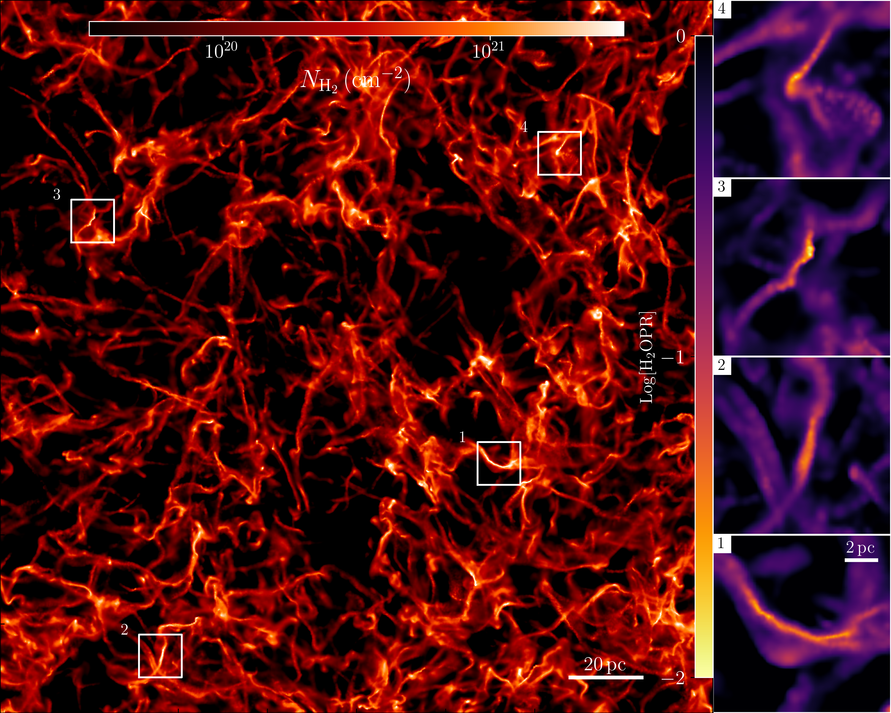
Figure 1: Column density map of H₂ at 4 Myr. On the right, we report the OPR^N in four filaments identified in the snapshot (corresponding to the four white squares in the left panel). The cloud already exhibits clear filamentary structures, and also some clumps forming within the most massive and largest ones. In these regions, the OPR is already low, with values typically below 0.1.

More in detail, in Table 1 we report the average properties of the four selected filaments (among the most massive and extended ones, i.e. $M>100\,\rm M_{\odot}$) at $t=4$ Myr. In particular, from left to right, we report the H₂ column density $N_{\rm H_{2}}$, the cosmic-ray ionisation rate $\zeta_{\rm H_{2}}$, the gas temperature $T_{\rm fil}$, the Mach number $\mathcal{M}$, the magnetic field $B$ magnitude, and two values for the OPR, i.e. OPR^N and the density-weighted line-of-sight average ratio OPR${}^{n}\equiv\langle n_{\rm o-H_{2}}\rangle/\langle n_{\rm p-H_{2}}\rangle$. Finally, in the last two columns, we report the mass per unit length $M/L$ and the filament width $W\equiv A_{\rm px}/L$, with $A_{\rm px}$ the effective pixel area of the dendrogram and $L$ the major axis length of the filament. In general, the filaments identified in our simulations show typical properties consistent with observations (Arzoumanian et al., 2011), i.e. lengths $L$ between 1 and 10 pc, axis ratios between 1:2 and 1:20, masses from a few tens up to a thousand solar masses, and, being still in an initial collapse stage, densities not exceeding $10^{4}\rm\,cm^{-3}$ with average temperatures around 30 K. The estimated mass per unit length ($M/L$) is compared with the critical value for collapse, obtaining a full spectrum of values ranging from $\sim 0.2$ (sub-critical) up to $\sim 3$ (super-critical), with the four reported in Table 1 lying around 1.0-1.5.

ID	$\log N_{\rm H_{2}}$	$n_{\rm H_{2}}$	$\log\zeta_{\rm H_{2}}$	$T_{\rm fil}$	$\mathcal{M}$	$B$	OPRN/n	$[M/L]$	$W$
	$(\rm\,cm^{-2})$	$(\rm cm^{-3})$	$(\rm\,s^{-1})$	$\rm(K)$	-	$(\mu\rm G)$	-	$\rm M_{\odot}pc^{-1}$	$(\rm pc)$
1	21.28	768.24	-15.53	31.4	10.60	7.60	0.10/0.06	77.56	0.10
2	21.28	1237.57	-15.54	28.0	3.55	10.13	0.08/0.03	54.09	0.12
3	21.22	1274.69	-15.58	23.9	7.78	9.92	0.06/0.01	41.33	0.16
4	21.38	2022.84	-15.51	28.3	6.14	9.30	0.06/0.03	52.70	0.08

Table 1: Main properties of four filaments out of hundreds in our fiducial simulation (cfr. Fig. 1) . From left to right, we report H₂ column density, average number density $n_{\rm H_{2}}$, average cosmic ray ionisation rate $\zeta_{\rm H_{2}}$, gas temperature $T_{\rm fil}$, Mach number $\mathcal{M}$, magnetic field magnitude $B$, OPR (using both column densities –first value– and average number densities – second value), mass per unit length $M/L$, and filament width $W$. All values we find are consistent with the expected ones derived from observations.

To further confirm the accuracy of our modelling which, being developed with ab-initio physics, has not been calibrated to reproduce real clouds, in Fig. 2 we compare our simulated cloud with observations of ‘diffuse’ clouds. In particular, we focus on properties connected to H₂ and its OPR, like the H${}_{3}^{+}$ abundance (top-left panel) and the cosmic-ray ionisation rate $\zeta_{\rm H_{2}}$ estimates (top-right panel) (Indriolo, 2012), the para–to–total ratio of H${}_{3}^{+}$ and H₂ (Crabtree et al., 2011) (bottom-left panel), and the water–to–HF column density ratio (bottom-right panel) (Sonnentrucker et al., 2015). The coloured two-dimensional histogram represents the full distribution of pixels (0.25 pc wide) in our simulation, the grey dots are the observed data, and the blue, orange, green, and red stars the average abundances from the identified filaments at different times. Finally, the magenta lines correspond to the theoretical abundance of H${}_{3}^{+}$ assuming a nascent distribution (solid line), in which the formation of H${}_{3}^{+}$ from cosmic ray-induced ionisation of H₂ fully determines the relative abundance of the nuclear spin values, and a thermalised distribution (dashed line), in which the relative abundance is dominated by collisional exchange between H${}_{3}^{+}$ and H₂ (Crabtree et al., 2011). The remarkable agreement suggests that our theoretical framework naturally produces reliable initial conditions for the collapsing filaments within molecular clouds (see Appendix C for a detailed analysis of the other simulations of our suite). In particular, in the bottom-left panel, both our simulation and observations lie in between the two theoretical curves, with our results more closely following the nascent distribution, which reflects the strong impact of cosmic rays. The abundance of water is slightly underestimated, particularly at high-density, likely because of the missing formation channels of water on dust grains in our network, which are potentially relevant in cold gas (Cazaux et al., 2010; Sonnentrucker et al., 2015).

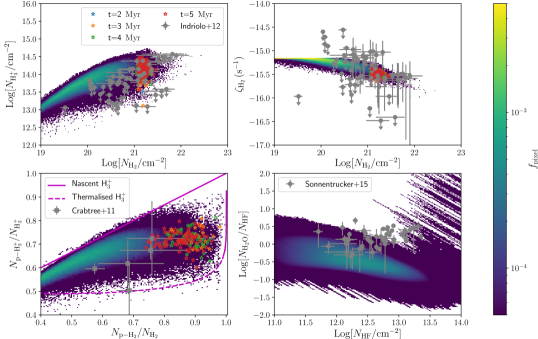
Figure 2: Comparison of our simulation with existing observations of diffuse clouds, shown as grey dots (Crabtree et al., 2011; Indriolo, 2012; Sonnentrucker et al., 2015). The top-left panel shows the abundance of H${}_{3}^{+}$ relative to H₂, the top-right panel the corresponding $\zeta_{\rm H_{2}}$, the bottom panel the para-to-total ratio for both H${}_{3}^{+}$ and H₂, and the bottom-right panel the H₂O relative abundance with respect to HF, where the HF column density in our simulation is extracted assuming a rigid scaling relative to H₂ (Indriolo, 2012) with scaling factors in the range $0.5\times 10^{-8}$–$3.5\times 10^{-8}$. Our simulation is in remarkable agreement with the observational results of most tracers, confirming the accuracy of our chemical and physical modelling, with only a slight discrepancy in H₂O, but still consistent with observations. This is likely attributed to the missing water formation channels on dust grains in our chemical network, which might be potentially important in cloud conditions (Cazaux et al., 2010; Sonnentrucker et al., 2015).

In order to disentangle whether time or density play the major role in producing these results, we report in Fig. 3 the evolution of the OPR distribution for every simulation element, as a function of the total hydrogen nuclei density. For this analysis, we directly use the local properties of the gas in the simulation, which allows us to avoid the dilution effects resulting from integrating along the line-of-sight (Ferrada-Chamorro et al., 2021). Each solid curve corresponds to a different time, with the error bars showing the 20th and 80th percentiles, whereas the black dashed line is the thermalised OPR, i.e. the balance between the ortho-to-para and para-to-ortho conversion, and the orange long-dashed one to the steady-state value, i.e. the ratio at chemical equilibrium self-consistently computed using our network. For completeness, we also show the total uncertainty resulting from our entire suite of simulations (see Appendix C) as a grey shaded area. We notice that the distribution extends to very low values ($\lesssim 0.1$) already at moderate densities ($n_{\rm H,tot}\sim 10^{3}-10^{4}\rm\,cm^{-3}$). Moreover, the distribution does not significantly change with time, suggesting that the OPR is mainly determined by density, with the dynamical evolution only being a second-order effect. This result suggests that, as soon as filaments form, the OPR is already well below 0.1, and that higher values found for OPR^N and from observations are hugely affected by dilution effects (by one order of magnitude or more). Our results are robust even against different physical assumptions (see Appendix C), with the upper limits (grey shaded area) still exhibiting very low OPR values when $n_{\rm H,tot}\gtrsim 10^{4}\rm\,cm^{-3}$. At low density, the ratio tightly follows the thermalised one, which is also consistent with the equilibrium value. As soon as the gas becomes fully molecular, instead, the distribution starts to differ, but still decreases towards very small values (0.001 or less). At the highest densities probed, the OPR in the simulation settles on the equilibrium value, which showed a moderate increase above $n_{\rm H,tot}\sim 10^{3}\rm\,cm^{-3}$, hence departing from the thermalised one.

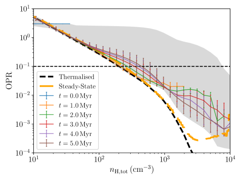
Figure 3: Three-dimensional distribution of the OPR as a function of $n_{\rm H,tot}$ at different times. The grey shaded area represents the uncertainty in the physical/chemical modelling in our suite of simulations (shown for completeness), the black dashed line corresponds to the thermalised ratio, valid for temperatures below $\sim$100 K (i.e. for densities larger than 30-40 cm^-3 in our specific case), and the orange long-dashed line to the equilibrium/steady-state value. We clearly see that time plays a minor role, with the distribution being almost uniquely determined by density. Most importantly, the OPR is already well below 0.1 above $10^{3}\rm\,cm^{-3}$, reaching 0.001 around $10^{4}\rm\,cm^{-3}$. Even in the most pessimistic case, dense gas above $10^{4}\rm\,cm^{-3}$ never exhibits OPR values above a few 0.01. The ratio follows the thermalised/steady-state value, starting to depart around $n_{\rm H,tot}\sim 100\rm\,cm^{-3}$, when the gas becomes fully molecular. However, at high densities, the OPR settles on the equilibrium value, which is much higher than the thermalised one.

4 Discussion and conclusions

In this work, we have performed 3D MHD simulations of a molecular cloud with state-of-the-art on-the-fly non-equilibrium chemistry, finding that filaments are characterised by already low OPR values. Our simulations show a remarkable agreement with available observations, without any a priori tuning of the model. It is important to remark that a proper comparison with other available works is difficult, as direct measurements or estimates of the OPR in diffuse and molecular clouds are rare. In particular, the few data in diffuse clouds (Crabtree et al., 2011) suggest values around 0.3-0.7, slightly higher than ours, but in relatively good agreement when considering the observational uncertainties (e.g. optical thickness of these lines and the possible dilution effects along the line-of-sight). Some indirect estimates in between 0.001-0.2 have also been provided for pre-stellar cores (Troscompt et al., 2009; Brünken et al., 2014; Pagani et al., 2013), i.e. in regions with densities higher than those explored by our simulations and representing an advanced stage of the star-formation process. However, the strong assumptions made to infer this fundamental quantity from different chemical proxies do not allow to get a reliable estimation from observations. In this context, our study represents a relevant step forward to improve the fundamental knowledge of the star-formation process.

The absence of sulfur chemistry in our work might represent a limitation, since it could reduce the ortho-to-para conversion efficiency by removing H⁺ via the reaction path S + H${}^{+}\to$ S⁺ + H (Furuya et al., 2015). However, Furuya et al. (2015) show that (i) sulfur is quickly adsorbed on dust grains as soon as S⁺ recombines and, as a consequence, (ii) this effect is relevant only for extremely high metal abundances, which are not compatible with the measured values of sulfur from observations. Hence, we assume that sulfur chemistry does not play a relevant role within the context of our model, and therefore it does not affect our conclusions.

Concluding, our state-of-the-art three-dimensional magneto-hydrodynamic simulations of molecular clouds formation with on-the-fly non-equilibrium chemistry indicate that the H₂ ortho-to-para ratio quickly evolves with density, reaching very low values (but far from the thermalised one) already at moderate densities typical of proto-filaments. This is particularly relevant for smaller scale studies, in which the unconstrained initial OPR is either varied in the allowed range to bracket its effect on the results (see, e.g. Sipilä et al., 2015; Kong et al., 2015; Bovino et al., 2020) or conservatively assumed to be around 0.1 (see, e.g. Jensen et al., 2021), i.e. larger than ours ($10^{-3}-10^{-2}$). The results in this work therefore establish that the initial conditions of the star formation process in filaments are characterised by already low OPR and typically high $\zeta_{\mathrm{H_{2}}}$, both conditions that would dramatically boost the deuteration mechanism and shorten the corresponding timescales. We notice that, even in filaments characterised by low cosmic ray ionisation rates (Indriolo, 2012), the expected OPR would be only moderately higher, and never as high as 0.1. For the first time, we have been able to determine the initial conditions of star-forming filaments from ab-initio conditions, in particular the chemical abundances of important species like H₂ (ortho- and para-), H${}_{3}^{+}$, CO, and H₂O, which have far-reaching implications for the deuteration process (hence on the reliability of chemical clocks), for the observed HDO/H₂O ratios in planet-forming regions (which strongly depends on the OPR), and its connection with the origin of water in our Solar System.

Appendix A Numerical methods

A.1 Turbulence driving

In order to drive turbulence in the box with properties similar to observed molecular clouds, the gas distribution is stirred by a random acceleration field obtained via an Ornstein–Uhlenbeck process (Federrath et al. 2010b; Bauer & Springel 2012). The energy power spectrum normalisation is set to obtain a velocity dispersion in the cloud $\sigma_{v}\sim 7\,\rm km\,s^{-1}$, and the auto-correlation time of the random process is set to $\tau=10$ Myr. Energy is injected only at large scales, according to a parabolic power spectrum peaking at $k=3$ (extending from $k=2$ up to $k=4$), assuming a half-solenoidal half-compressive driving (Bauer & Springel 2012). This assumption is reasonably consistent with recent simulations of molecular cloud formation in which turbulence was driven self-consistently via random supernova explosions (Padoan et al. 2016). During this relaxation phase, which lasts for 50 Myr in order to let turbulence fully develop, we do not include self-gravity, and we assume an isothermal equation of state with $T=5000$ K and no chemistry evolution (Mandal et al. 2020). This allows us to start the self-consistent evolution of the cloud with ab-initio chemical abundances typical of the warm neutral medium, avoiding any pre-processing of the species during the relaxation. Nevertheless, to further corroborate our results and isolate the effect of self-gravity, we also perform an additional experiment in which chemistry and proper cooling are already included during the relaxation phase.

A.2 Sink formation

Near the end of the simulation, we expect clumps to form in filaments and a few resolution elements to reach very high densities, thus requiring very short time-scales to integrate the dynamics. In order to avoid this undesired slow-down and let the simulation to evolve for longer times, we convert the gas hitting the resolution limit of the simulation into proto-stellar objects, commonly dubbed ‘sink particles’, which are able to grow via accretion of surrounding gas. In this work, we include a simple sink formation scheme, i.e. gas particles i) above $n_{\rm H,tot}>10^{10}\rm\,cm^{-3}$ ii) showing negative velocity divergence and iii) located at a relative gravitational potential minimum are converted into sink particles, unless another sink is found within their kernel volume. After a sink has formed, we allow it to accrete gas within its kernel volume, corresponding to a sphere enclosing an effective number of 32 neighbours that matches the sink formation conditions. However, since our main interest is in the pre-stellar phase, rather than in the star formation process itself, we stop our simulations after a few sinks have formed in the box, making the details of the sink formation scheme almost irrelevant.

A.3 Cosmic ray flux determination

The cosmic ray ionisation rate in molecular clouds is affected by several uncertainties, since it strongly depends on the physical conditions inside and outside the cloud. For this reason, most studies to date explore different values of the cosmic ray ionisation rate $\zeta_{\rm H_{2}}$ typically in the range $1.3\times 10^{-17}-1.3\times 10^{-16}$. While, in some of our simulations we also employ a constant value, in a real cloud cosmic rays are attenuated as they move deeper into it, hence a more consistent modelling should take into account this aspect. However, detailed cosmic ray propagation in 3D simulations is computationally expensive, and would add an additional layer of complexity to our already computationally expensive simulations. For this reason, in this work we opt for an effective model which, starting from the local properties of each resolution element, allows us to follow the variations of $\zeta_{\rm H_{2}}$ in the cloud, at a moderate computational cost(Padovani et al. 2018):

$$\zeta_{\rm H_{2}}=\zeta_{\rm H_{2},p}+\zeta_{\rm H_{2},e},$$ (1)

where the two contributions are from protons and electrons, respectively, and are defined as

$$\zeta_{\rm H_{2},p} = \left\{\begin{array}[]{cc}6.8\times 10^{-16}N_{20}^{-0.423}&N_{\rm eff}<10^{25}\rm cm^{-2}\\ 5.4\times 10^{-18}\exp(-\Sigma_{\rm eff}/38)&{\rm otherwise}\end{array}\right.$$ (4)

$$\zeta_{\rm H_{2},e} = \left\{\begin{array}[]{cc}1.4\times 10^{-19}N_{20}^{-0.04}&N_{\rm eff}<10^{25}\rm cm^{-2}\\ 3.3\times 10^{-20}\exp(-\Sigma_{\rm eff}/71)&{\rm otherwise}\end{array}\right.$$ (7)

where $N_{20}=N_{\rm eff}/10^{20}\rm\,cm^{-2}$ and $\Sigma_{\rm eff}=2.36m_{\rm H}N_{\rm eff}$, with $N_{\rm eff}$ the effective column density traversed by cosmic rays. To determine $N_{\rm eff}$, we assume that the magnetic field lines are relatively not curved (as expected in this earlier star-formation stage) and they have small intensity variations, allowing us to consider the total column density $N_{\rm H_{2}}=N_{\rm o-H_{2}}+N_{\rm p-H_{2}}$ as a reliable first-order approximation, which we determine using a local approximation (Grassi et al. 2017b) in which $N_{x}=1.87\times 10^{21}(n_{x}/10^{3}\rm\,cm^{-3})^{2/3}$, of $N_{\rm eff}$. When the magnetic field lines are not straight, our estimate of $N_{\rm eff}$ represents a lower limit to the actual value, which translates into our cosmic ray ionisation rate being an upper limit. This is why, in our suite, we chose an average model among those in the literature (Padovani et al. 2009), and also explored very different conditions, i.e. a conservative and uniform $\zeta_{\rm H_{2}}=1.3\times 10^{-17}$ s^-1, and the locally varying one, to bracket the possible conditions of real clouds.

A.4 Ortho-to-para H₂ conversion on dust

Recent experimental works both on amorphous solid water(Ueta et al. 2016) as well as on bare silicates(Tsuge et al. 2021), show the efficiency of the ortho-to-para H₂ conversion on the surface of dust grains. To consistently follow this process within our simulations and evaluate its overall impact on the OPR, we employ state-of-the-art frameworks(Bovino et al. 2017; Furuya et al. 2019), in which the conversion rates in units of s^-1 are defined as

$$k_{\mathrm{op}}=k_{\mathrm{ads}}^{\mathrm{oH_{2}}}\eta_{\mathrm{op}}$$ (8)

$$k_{\mathrm{po}}=k_{\mathrm{ads}}^{\mathrm{pH_{2}}}\eta_{\mathrm{po}}$$ (9)

where the $k_{\mathrm{ads}}^{i}=Sv_{i}\sigma_{\mathrm{dust}}$ are the adsorption rates of the species on the surface of grains, with $S$ being the sticking coefficient (here assumed to be 1 for simplicity), $v_{i}$ the thermal gas speed, and $\sigma_{\mathrm{dust}}$ the distribution-averaged grain geometrical cross-section. The efficiency of the process is regulated by the factor $\eta_{i}$ which represents the competition between the conversion process and desorption, and it is defined as(Furuya et al. 2019)

$$\eta_{\mathrm{op}}=\frac{t_{\mathrm{des}}}{t_{\mathrm{des}}+\tau_{\mathrm{conv}}}\frac{1}{1+\gamma}$$ (10)

$$\eta_{\mathrm{po}}=\frac{t_{\mathrm{des}}}{t_{\mathrm{des}}+\tau_{\mathrm{conv}}}\frac{\gamma}{1+\gamma}$$ (11)

where the desorption time is calculated as the minimum between the thermal desorption time and the cosmic-ray induced desorption time, $\tau_{\rm conv}$ is the experimental conversion time(Tsuge et al. 2021), fitted as $\tau_{\mathrm{conv}}=6.3\times 10^{4}T_{\mathrm{dust}}^{-1.9}$, and $\gamma=9\exp{(-170.5/T_{\mathrm{dust}})}$ is the thermalised value of the ortho-to-para H₂ ratio, assuming the energy difference between o‐H₂ and p‐H₂ on the grains is the same as that in the gas phase. This allows us to include in the H₂ rate equations both the ortho-to-para conversion and its inverse process (para-to-ortho). However, since the inverse process is in general negligible at low temperatures(Bovino et al. 2017), we opt for completely neglecting it in our simulations, which in practice corresponds to assuming $\gamma=0$ (Bovino et al. 2017). We note that our approach is based on a single average binding energy approximation, in particular $E_{b}=600$ K as reported in literature(Perets & Biham 2006; Vidali & Li 2010; He & Vidali 2014), and refer to other recent works(Furuya et al. 2019) for a more comprehensive treatment which also includes the thermal hopping between different adsorption sites. The effect of these processes on the evolution of the H₂ OPR is discussed in Appendix C.

A.5 HF abundance in diffuse clouds

Observations of water in diffuse clouds typically lack a direct measure of the H₂ column density, using instead HF (or other hydrides) as an alternative proxy(Sonnentrucker et al. 2015). Despite the correlation $N_{\rm HF}=\chi_{\rm HF}N_{\rm H_{2}}$ is found to be quite tight, the uncertainty in the conversion factor reaches up to a factor of $\sim 7$, ranging from $0.5\times 10^{-8}$ up to $3.5\times 10^{-8}$ (Indriolo 2012). For this reason, and considering the fact that our chemical network does not include HF, no simple comparison between simulations and observations exists, and particular attention must be taken when converting H₂ to HF (or viceversa). For the comparison between our runs and observations of Fig. 2, we opt therefore for a more sophisticate procedure, i.e. for each value of $N_{\rm H_{2}}$ in our simulations, we estimate the $N_{\rm HF}$ using 100 different values of $\chi_{\rm HF}$ within the observed range, so that this source of uncertainty is properly accounted for, and combine all these measures in a single 2D histogram reported in the bottom-right panel of the figure, appropriately normalised to the total number of measures available.

Appendix B Relaxation phase

Our simulation suite is composed of four runs, three of them starting from our fiducial isothermal relaxation without chemistry, that we call RelaxIso and one in which proper cooling and chemistry are accounted for also during relaxation, that we call RelaxChem, in which $\zeta_{\rm H_{2}}=1.3\times 10^{-17}$ s^-1 is kept constant over time in the entire box. The relaxation phase is necessary to guarantee that turbulence fully develops in the box, producing initial conditions of the actual simulations that more closely represent realistic molecular clouds(Federrath et al. 2010a). To give an idea of the global evolution of our fiducial simulated cloud, we show in Fig. 4 the main properties of the box during both the relaxation phase (reported as a grey shaded area with negative times) and the actual run (reported with positive times), i.e. the density-weighted average 3D velocity dispersion $\sigma_{\rm v}$, sound speed, Mach number, $\beta=P/P_{\rm B}$ parameter, with $P=\rho c_{s}^{2}$ the thermal pressure (with $\rho$ the total gas density) and $P_{\rm B}=\langle B\rangle^{2}/(8\pi)$ the magnetic pressure, and virial parameter $\alpha_{\rm vir}=5\sigma_{\rm v}^{2}L/(3GM)$, with $L$ the box size and $M$ the box total mass. During the relaxation phase, $\sigma_{\rm v}$ increases up to the desired value as a result of turbulence driving, whereas the sound speed stays constant, because of the constant temperature assumption, which also reflect in the virial parameter increase to about 1.5 and the Mach number staying close to unity. The modest change in density distribution results in a small decrease of the average magnetic field, and the corresponding increase of $\beta$ by a factor of two. After relaxation, $\sigma_{\rm v}$ only modestly varies, while $c_{s}$ significantly decreases because of cooling, producing a rapid increase of $\mathcal{M}$ to the typically observed values. These variations reflect directly on $\beta$ and $\alpha_{\rm vir}$, except for the magnetic field that suddenly rises above 10 $\mu$G around $t=5$ Myr, when a large portion of the gas starts to collapse.

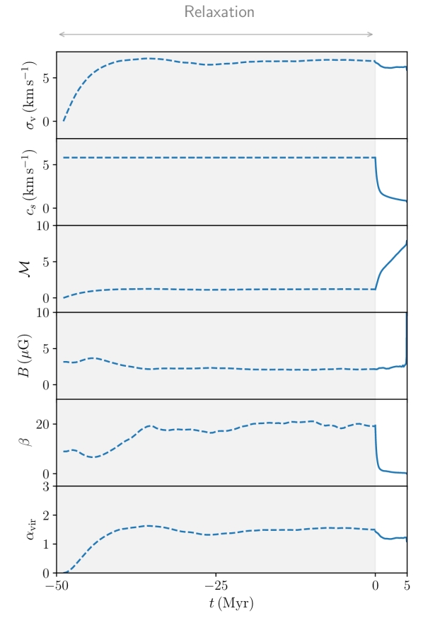
Figure 4: Evolution of the global properties of the turbulent cloud in our fiducial model, during the relaxation phase (shaded area with negative times) and the actual run (positive times). While turbulence leads to an initial increase of $\sigma_{\rm v}$ (reflected in all the other properties it affects), the sound speed remains constant during relaxation, producing a Mach number slightly above unity. During the run, instead, $\mathcal{M}$ increases quickly to the typically observed values, because of cooling. On average, the magnetic field does not change significantly, as long as the typical density interval remains small.

Model	$\langle n_{\rm H,tot}\rangle$	$\langle T\rangle$	$\langle\sigma_{v}\rangle$	$c_{s}$	$\mathcal{M}$	$\langle\beta\rangle$	$\alpha_{\rm vir}$
	$(\rm cm^{-3})$	$(\rm K)$	$(\rm kms^{-1})$	$(\rm kms^{-1})$	-	-	-
RelaxChem	$123.8$	$128$	$7.525$	$0.663$	$11.35$	$0.318$	$1.761$
RelaxIso	$6.2$	$5\times 10^{3}$	$7.162$	$5.820$	$1.230$	$2.008$	$1.600$

Table 2: Main properties of our turbulent box after 50 Myr of relaxation for the two different considered models RelaxIso and RelaxChem. The inclusion of cooling and chemistry during the relaxation phase allows the gas to spread over a larger density/temperature interval, resulting in very different thermal properties (typical of colder and denser gas), whereas those fully determined by turbulence remain almost identical (the 3D velocity dispersion $\sigma_{\rm v}$ and the virial parameter $\alpha_{\rm vir}$).

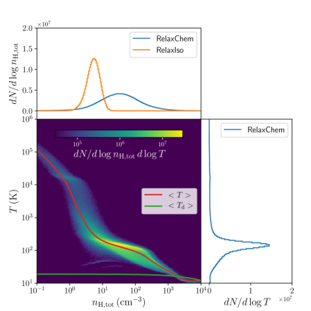
Figure 5: Distribution of the gas at the end of the relaxation phase. The density–temperature diagram corresponds to RelaxChem (notice that this distribution does not change when gravity is included, apart from extending to higher densities as the gas collapses), with the red line representing the average temperature, and the green one the average dust temperature. The temperature-only distribution in the right-hand panel shows the typical temperature of the gas, 100-200 K, higher than the typical temperature assumed in isothermal molecular cloud simulations. In the top panel, we show instead the density distribution for both relaxation models, where RelaxChem, extending to higher densities because of cooling, is shown in blue, and RelaxIso, more concentrated around the initial density, in orange.

For completeness, we also report in Table 2 the same main properties at the end of the relaxation phase for the two relaxation models we considered, in addition to the density-weighted average density and temperature. While the turbulence-driven properties are the same in both relaxation models, the thermodynamic is not, resulting in very different average temperatures and densities. To better clarify how the gas is distributed in the two cases, in Fig. 5 we show the density and temperature distributions (the latter only for the RelaxChem case). Overlaid on the density-temperature plot of RelaxChem we also report the average temperature (red) and dust temperature (green) curves, that differ significantly at low density, while couple at $n_{\rm H,tot}\sim 10^{4}\rm\,cm^{-3}$. In the right panel, we show the temperature-only distribution, which peaks around 100–200 K, at which most of the ‘diffuse’ gas settles. In the top panel we report instead the density-only distribution, in this case also for RelaxIso (orange histogram). As expected, in RelaxChem, gas cooling allows the gas to get denser after turbulence-induced compression, spreading over a larger density interval, that follows a Gaussian-like profile (the typically expected Log-Normal density probability distribution function). On the other hand, RelaxIso keeps the gas to moderate densities, producing a much narrower distribution centred around the average density of the initial conditions.

Appendix C The full simulation suite

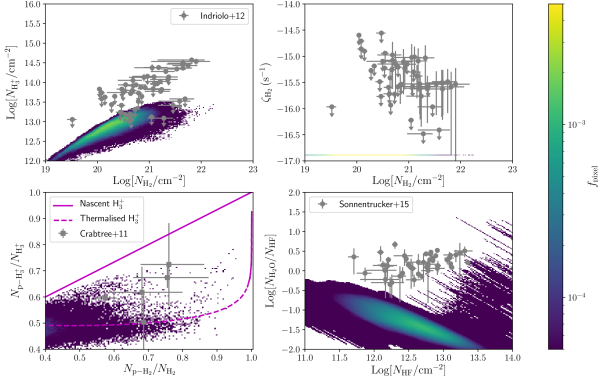
Figure 6: Same as Fig. 2 for model RelaxIso_SG. Unlike in our fiducial model, here the abundances are much lower than those observed, consistently with the huge difference in $\zeta_{\rm H_{2}}$ between the observationally-inferred value and the one in the simulation. In this case, the data in the bottom panel are in better agreement with the thermalised distribution, because of the small effect of cosmic ray-induced ionisation of H₂ relative to atom exchange reactions.

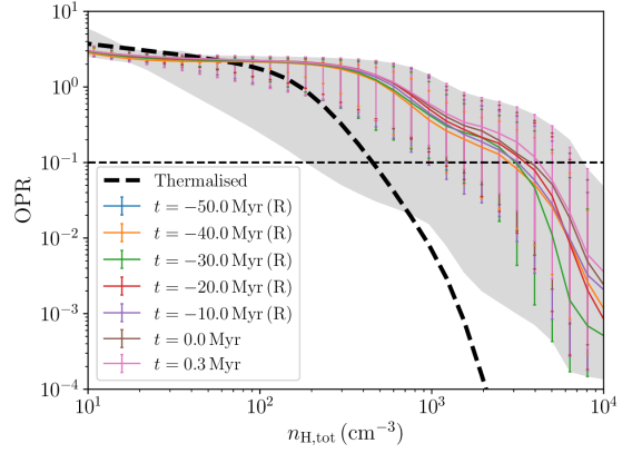
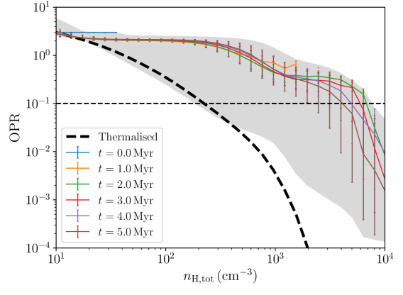
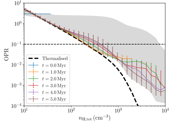
Figure 7: Same as Fig. 3 for models RelaxChem_SG (top panel), RelaxIso_SG (middle panel), and RelaxIso_SG_OPdust (bottom panel). The OPR distribution shows very mild variations with time in all cases but, while the bottom panel shows almost no difference with the fiducial model, the other two runs are typically offset upwards, a result that reflects the very low cosmic ray ionisation rate, not typical of molecular cloud conditions. Nevertheless, the OPR at $n_{\rm H,tot}\sim 10^{4}\rm\,cm^{-3}$ is always well below 0.1.

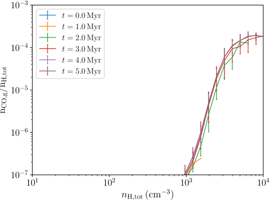
Figure 8: Fraction of CO in gas phase in our fiducial model, as a function of total hydrogen density. Despite the high $\zeta_{\rm H_{2}}$, CO is able to form efficiently, reaching the canonical abundance in gas above $n_{\rm H,tot}=3-4\times 10^{3}\rm\,cm^{-3}$. We also notice freeze-out on dust grains starting to deplete CO at $n_{\rm H,tot}\sim 10^{4}\rm\,cm^{-3}$, as expected, although the number of resolution elements above this density is very low. We also find that the abundance does not significantly vary with time, similarly to the OPR, as long as depletion remains almost negligible.

The four simulations we performed are meant to cover most of the plausible parameter space, thus properly constraining our models relative to observations. In particular, compared to our fiducial model, we consider: a) RelaxChem plus self-gravity, named RelaxChem_SG, b) RelaxIso plus self-gravity, named RelaxIso_SG, c) the fiducial model (see Main Text), and d) the fiducial model with the addition of ortho–to–para conversion on dust (as described in Section A), named RelaxIso_CR_OPdust. Similar to Fig. 3 in the Main Text, Fig. 7 reports the OPR evolution for models RelaxChem_SG (top panel), RelaxIso_SG (middle panel), and RelaxIso_SG_OPdust (bottom panel) for completeness. RelaxIso_CR_OPdust gives almost identical results to our fiducial model, suggesting that the OPR conversion on dust, which slightly accelerates the ortho-to-para conversion, does not change our picture significantly, and that the gas-phase collisions with H⁺ and H${}_{3}^{+}$ are already efficient enough to bring the OPR down, without the need of this additional mechanism. For RelaxChem_SG, in which chemistry is also evolved during the relaxation phase, the OPR distribution in these stages is reported with negative times and an additional ‘(R)’ in the label. We immediately see that, even without self-gravity, when cooling is included, the denser gas stirred by turbulence quickly settles on a steady-state OPR distribution, and the addition of gravity does not alter the distribution at all. Compared to the fiducial run, here the OPR is typically higher, farther from the thermalised value. Nevertheless, a clear drop can be observed around $n_{\rm H,tot}\sim 3-4\times 10^{3}\rm\,cm^{-3}$, which also in this case yields an OPR well below 0.1 at the typical densities of star-forming filaments ($n_{\rm H,tot}\gtrsim 10^{4}\rm\,cm^{-3}$). A similar trend can be observed in RelaxIso_SG, although the high density drop is even steeper that in the previous case, consistent with the weak time-dependence of the distribution (notice indeed that in this second case chemistry was not present during the initial relaxation, hence the processing time is much shorter). Combining the results of these two models, we can conclude that the higher OPR distribution relative to our fiducial model is the result of the very low cosmic ray ionisation rate, which is reasonable for protostellar cores, but not for the typical conditions of molecular clouds(Padovani et al. 2009, 2018). Nonetheless, all our models, even the most pessimistic ones, result in low OPR ($\lesssim 0.01)$ at the typical densities of star-forming filaments, and this further corroborates our conclusions in the Main Text. To further support our claims about the effect of a too low $\zeta_{\rm H_{2}}$, we compare in Fig. 6 our RelaxIso_SG with observations, as in Fig. 2. We immediately see that, with respect to our fiducial run, the results here are completely off, with the simulation yielding lower abundances than those observed. This is perfectly consistent with the discrepancy between our assumed $\zeta_{\rm H_{2}}$ with respect to the observationally-inferred value (Indriolo 2012), even though these results might be compatible with the claimed non-detections. Moreover, in the bottom-left panel, our results almost perfectly lie on the thermalised distribution, consistently with the fact that cosmic ray-induced ionisation of H₂ becomes almost negligible with respect to the atom exchange reactions dominating in thermalised conditions.

Despite not being the focus of this study, we report in Fig. 8 the abundance of gaseous CO in our fiducial simulation for completeness at different times. CO forms efficiently in our filaments, reaching the canonical fraction of about $10^{-4}$, despite the high cosmic ray ionisation rate. We also notice that CO does not exhibit any strong time-dependence in the probed density range, but this is not surprising since freeze-out on dust grains still has a negligible impact.

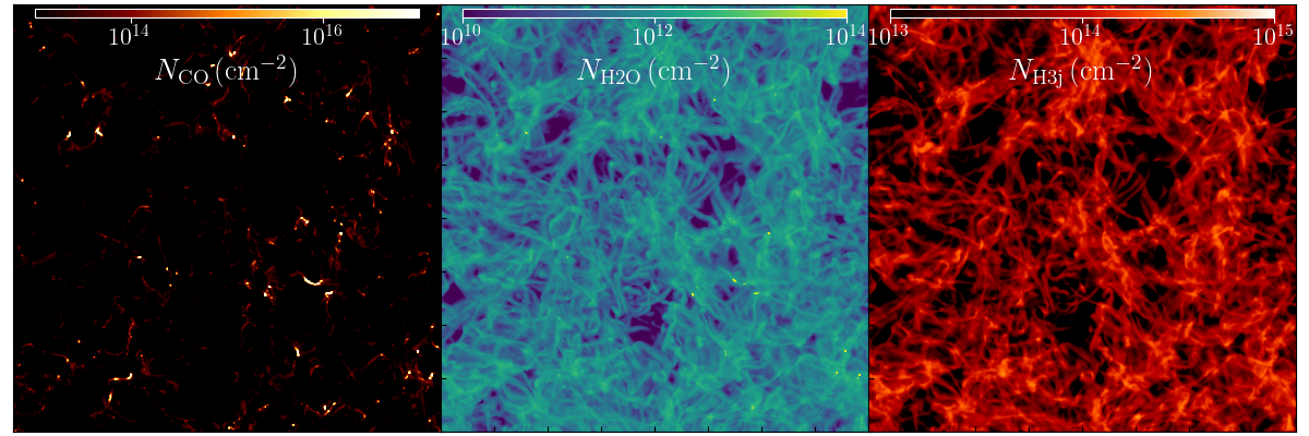
Figure 9: Examples of column density maps of three important chemical species in molecular clouds, i.e. CO, H₂O, and H${}_{3}^{+}$ respectively, from left to right. While H${}_{3}^{+}$ is quite uniformly distributed in the box, H₂O forms in larger amounts in moderately higher density gas, and CO reaches typically observed values ($N_{\rm CO}\gtrsim 10^{17}\rm\,cm^{-2}$) only in proto-filaments (notice the huge difference, about 4 orders of magnitude, between the filaments and the background).

As a final example of the unprecedented level of detail of our simulations including on-the-fly complex chemistry, we also report in Fig. 9 the column density maps of relevant chemical species that are directly tracked in our simulations, i.e. CO, H₂O, and H${}_{3}^{+}$ from left to right. CO is the mostly concentrated species, and appears in large amounts only in dense gas (proto-filaments), with the background reaching at most a 4 orders of magnitude lower abundance. Water (and especially H${}_{3}^{+}$) are instead more uniformly distributed, showing mild variations across very different density conditions.