We present a new set of parton distribution functions (PDFs) based on a fully global dataset and machine learning techniques: NNPDF4.0. We expand the NNPDF3.1 determination with 44 new datasets, mostly from the LHC. We derive a novel methodology through hyperparameter optimization, leading to an efficient fitting algorithm built upon stochastic gradient descent. We use NNLO QCD calculations and account for NLO electroweak corrections and nuclear uncertainties. Theoretical improvements in the PDF description include a systematic implementation of positivity constraints and integrability of sum rules. We validate our methodology by means of closure tests and “future tests” (i.e. tests of backward and forward data compatibility), and assess its stability, specifically upon changes of PDF parametrization basis. We study the internal compatibility of our dataset, and investigate the dependence of results both upon the choice of input dataset and of fitting methodology. We perform a first study of the phenomenological implications of NNPDF4.0 on representative LHC processes. The software framework used to produce NNPDF4.0 is made available as an open-source package together with documentation and examples.

1 Introduction

It is now an accepted fact that frontier high-energy physics at colliders requires percent-level accuracy both in theory and experiment [1]. On the theoretical side, the two main obstacles to achieving this are missing higher order corrections in perturbative computations [2], and uncertainties in parton distribution functions (PDFs) [3, 4]. The main aim of this paper is to show how percent-level accuracy might be achieved for PDFs.

The most recent set of PDFs determined by NNPDF, NNPDF3.1 [5], was the first to extensively include LHC data, and was able to reach 3-5% precision in the PDF uncertainties. It was based on NNPDF3.x fitting methodology, the first to be validated by means of closure tests, thereby ensuring that this precision was matched by a comparable accuracy.

The NNPDF4.0 PDF set presented here is a major step forward in three significant aspects: i) the systematic inclusion of an extensive set of run I LHC at 7 and 8 TeV data and, for the first time, of LHC Run II data at $\sqrt{s}=13$ TeV and of several new processes not considered before for PDF determinations; ii) the deployment of state-of-the-art machine learning algorithms which result in a methodology that is considerably faster and leads to more precise PDFs; iii) the validation of these PDF uncertainties both in the data and in the extrapolation regions using closure and future tests.

All in all, the main accomplishment of this new PDF set is to go one step further in achieving the main goal that motivated the NNPDF methodology in the first place [6], namely, to reduce sources of bias in PDF determination. The use of a wider dataset reduces sources of bias that might be related to the dominance of a particular process. The use of a machine learned methodology reduces sources of bias related to methodological choices, that are now mostly made through an automated procedure. Finally, the extensive set of validation tools explicitly checks the absence of bias: in fact, “future tests”, to be discussed below, can expose the historical bias that was present in previous PDF determinations.

The NNPDF4.0 global analysis includes 44 new datasets in comparison with NNPDF3.1. These involve a number of new LHC measurements of processes already present in NNPDF3.1, but also data from several new processes, whose impact on PDFs has been the object of dedicated studies. Specifically, direct photon production (studied in Ref. [7]), single-top production (studied in Ref. [8]), dijets (studied in Ref. [9]), $W$+jet (studied in Ref. [10]), and deep-inelastic jet production. A significant consequence of this extension of the dataset is that now the PDFs are largely controlled by LHC data: unlike in the past, a DIS-only PDF determination leads to much larger uncertainties and visibly different results.

NNPDF4.0 is the first PDF determination based on a methodology that is selected automatically rather than through manual iterations and human experience. All aspects of the neural network PDF parametrization and optimization (such as neural net architecture, learning rates or minimization algorithm) are selected through a hyperparameter optimization procedure [11], an automated scan of the space of models that selects the optimal methodology. A quality control method is used in order to make sure that the optimization does not produce a methodology that leads to overfitted PDFs. This is done through $K$-folding [6], checking iteratively the effectiveness of any given methodology on sets of data excluded in turn from the fit. All this is made possible by a speedup of the NNPDF fitting code, which is now able to fit an individual replica about twenty times faster, thanks mostly to the use of stochastic gradient descent methods provided by the TensorFlow library, rather than through the genetic algorithm minimization used previously, along with various technical improvements to be discussed below [11, 12, 13].

The widening of the dataset (with fixed methodology), and especially the methodological improvements (with fixed dataset) lead to a reduction of PDF uncertainties, so their combination brings us close to percent precision. This demands a careful validation of these uncertainties, which is achieved by means of two classes of tests.

The first is closure tests, already introduced in NNPDF3.0 [14], which here are considerably extended and systematized, thanks to the much greater fitting efficiency. These consist of fitting PDFs to pseudo-data generated assuming a certain underlying true PDF, and comparing the result of the fit to the known true PDF by means of suitable statistical estimators. The closure test verifies that PDF uncertainties are faithful, specifically in comparison to the data used to fit them. The second is future tests [15]: these compare the results obtained fitting PDFs to a subset of the data, which covers a small kinematic region compared to the full dataset. For example, PDFs are fitted to a pre-HERA dataset, and the result is compared to LHC data. The future test verifies that PDF uncertainties are faithful when extrapolated outside the region of the data used to fit them.

As a further test of methodological reliability, we study the robustness of results upon methodological variations, and in particular we show that PDFs are stable upon changes of the parametrization basis (i.e. the particular linear combination of PDFs that is parametrized by neural nets), thereby confirming that results are parametrization-independent.

NNPDF4.0 PDFs also include a number of improvements at all stages of the PDF determination procedure. The most relevant ones are the following:

• While the main PDF determination is performed with NNLO QCD (with further sets provided at NLO and LO), NLO electroweak (EW) and mixed QCD-EW processes are implemented for all LHC processes using recent dedicated tools [16] and assessed both for phenomenology and in the determination of the input dataset to be used for PDF fitting.

• Whenever heavy nuclear or deuteron targets are involved, nuclear effects are accounted for as theoretical uncertainties using the methodology of Refs. [17, 18, 19], and the results of the nNNPDF2.0 nuclear PDF determination [20].

• Strict positivity of $\overline{\rm MS}$ PDFs is implemented following the results of Ref. [21].

• Finiteness of non-singlet baryon number, i.e., integrability of all non-singlet PDF first moments is enforced. This specifically implies finiteness of the Gottfried sum [22] $U-D$ and of the strangeness sum $U+D-2S$, where $U$, $D$ and $S$ denote respectively the first moment of the sum of quark and antiquark PDFs for up, down and strange quarks.

• The selection of a consistent dataset is based on an objective two-stage procedure. Potentially problematic datasets are identified on the basis of either poor compatibility with the global dataset, or indications of instability of their experimental covariance matrix. These datasets are then subjected in turn to a dedicated fit in which the failed dataset is given a large weight, and then accepted or rejected depending on the outcome.

The main missing features of the current PDF determination, which are left for future work, are the inclusion of theory uncertainties (specifically missing higher order corrections), which could be done using the methods of Refs. [23, 24], and the full inclusion of EW and mixed QCD-EW corrections directly at the fitting level, which will be possible using the tools of Ref. [16].

The NNPDF4.0 PDF set is released at LO, NLO and NNLO QCD, for a variety of values of $\alpha_{s}$. The default PDF sets are provided in the FONLL variable-flavor number scheme [25] with maximum number of flavors $n_{f}=5$, and an independently parametrized charm PDF. PDF sets with different maximum number of flavors and with a perturbatively generated charm PDF are also made available, along with PDF sets determined using reduced datasets, which may be useful for specific applications. The main sets are delivered in the following formats: a Monte Carlo representation with 1000 replicas; a Hessian set with 50 eigenvectors obtained from the Monte Carlo set via the MC2Hessian algorithm [26, 27]; and a compressed set of 100 Monte Carlo replicas, obtained from the original 1000 through the Compressor algorithm [28] as implemented in the new Python code of Ref. [29]. The final NNPDF4.0 NNLO PDFs are shown in Fig. 1.1 both at a low ($Q=3.2$ GeV) and a high ($Q=100$ GeV) scale.

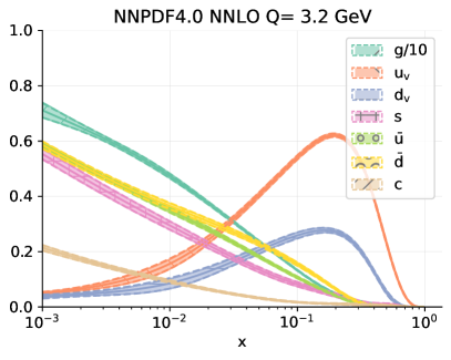
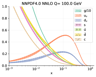
Figure 1.1: The NNPDF4.0 NNLO PDFs at $Q=3.2$ GeV (left) and $Q=10^{2}$ GeV (right).

More importantly, the full NNPDF software framework is released as an open source package [30]. This includes the full dataset; the methodology hyperoptimization; the PDF parametrization and optimization; the computation of physical processes; the set of validation tools; and the suite of visualization tools. The code and the corresponding documentation are discussed in a companion paper [31].

The structure of this paper is the following. First, in Sect. 2 we present the input experimental data and the associated theoretical calculations that will be used in our analysis, with emphasis on the new datasets added in comparison to NNPDF3.1. Then in Sect. 3 we discuss the fitting methodology, in particular the parametrization of PDFs in terms of neural networks, their training, and the algorithmic determination of their hyperparameters. The procedure adopted to select the NNPDF4.0 baseline dataset is described in Sect. 4. The main result of this work, the NNPDF4.0 determination of parton distributions, is presented in Sect. 5, where we also compare with previous NNPDF releases and with other PDF sets. The closure test and future test used to validate the methodology are described in Sect. 6.

Subsequently, we assess the dependence of our PDFs on the dataset in Sect. 7, where we study the impact of new data in comparison with NNPDF3.1, and verify the impact of individual processes by studying PDF determinations in which data corresponding to individual classes of processes are removed in turn. Also, we present PDFs determined by adding specific datasets, such as the EMC charm structure function, the NOMAD neutrino dimuon structure functions, and the HERA DIS jet data. Then in Sect. 8 we assess the dependence of PDFs on the methodology and verify the robustness of our results, by comparing with PDFs obtained using the previous NNPDF3.1 methodology and by studying the impact of new positivity and integrability constraints, checking the independence of results of the choice of PDF parametrization, discussing the impact of independently parametrizing the charm PDF, and studying the role of nuclear corrections. We finally present a first assessment of the implications of NNPDF4.0 for LHC phenomenology in Sect. 9, by computing PDF luminosities, fiducial cross-sections, and differential distributions for representative processes. In Sect. 10 we summarize and list the NNPDF4.0 grid files that are made available through the LHAPDF interface [32] and provide a summary and outlook.

A brief overview of the NNPDF fitting code is presented in App. A, while a more extensive description is provided by the companion publication [31]. In App. B we compare the NNPDF4.0 dataset to that adopted in other PDF determinations.

2 Experimental and theoretical input

We present the NNPDF4.0 dataset in detail. After a general overview, we examine each of the processes for which new measurements are considered in NNPDF4.0, we present the details of the measurements, and, for each dataset, we describe how the corresponding theoretical predictions are obtained. In NNPDF4.0, theoretical predictions for data taken on nuclear targets are supplemented by nuclear corrections, which are specifically discussed in a dedicated section. Experimental statistical and systematic uncertainties are treated as in previous NNPDF determinations: see in particular Sect. 2.4.2 of Ref. [14] for a detailed discussion.

The global dataset presented in this section is the basis for the final NNPDF4.0 dataset, which will be selected from it by applying criteria based on testing for dataset consistency and compatibility, and for perturbative stability upon the inclusion of electroweak corrections. The selection of the final dataset will be discussed in Sect. 4 below.

2.1 Overview of the NNPDF4.0 dataset

The NNPDF4.0 dataset includes essentially all the data already included in NNPDF3.1, the only exceptions being a few datasets that are replaced by a more recent final version, and single-inclusive jet datasets which are now partly replaced by dijet data, as we discuss below. All the new datasets that were not included in NNPDF3.1 are more extensively discussed in Sect. 2.2. For all those already included in NNPDF3.1 we refer to Sect. 2 of Ref. [5] for a detailed discussion. Nevertheless we give a summary below.

The NNPDF3.1 dataset included data for lepton-nucleon, neutrino-nucleus, proton-nucleus and proton-(anti)proton scattering processes. The bulk of it consisted of deep inelastic scattering (DIS) measurements: these included fixed-target neutral current (NC) structure function data from NMC [33, 34], SLAC [35] and BCDMS [36], fixed-target inclusive and dimuon charged current (CC) cross-section data from CHORUS [37] and NuTeV [38, 39], and collider NC and CC cross-section data from the HERA legacy combination [40]. The combined H1 and ZEUS measurement of the charm cross-section [41] and the separate H1 [42] and ZEUS [43] measurements of the bottom cross-section were also included, both to be replaced by more recent data as we discuss below. The charm structure function measured by the EMC experiment [44] was also studied in a variant fit, in which its constraining power on the intrinsic component of the charm PDF was explicitly assessed, and the same will be done here.

In addition to the DIS measurements, the NNPDF3.1 dataset included fixed-target DY data from the Fermilab E605 [45] and E866 [46, 47] experiments, inclusive gauge boson production [48, 49, 50, 51] and single-inclusive jet production [52] cross-section data from the Tevatron. A sizable amount of LHC data were also included, specifically: inclusive gauge boson production data from ATLAS [53, 54, 55, 56], CMS [57, 58, 59, 60] and LHCb [61, 62, 63, 64]; $Z$-boson transverse momentum production data from ATLAS [65] and CMS [66]; and top pair production total and differential cross-section data from ATLAS [67, 68, 69] and CMS [70, 71, 72]. Single-inclusive jet production data from ATLAS [73, 74, 75] and CMS [76, 77] were also included. These will be partly replaced by dijet data as we discuss below. For the determination of NLO PDFs, $W$ production measurements in association with a charm jet from CMS [78] were also included. Most of these LHC measurements were performed at $\sqrt{s}=7$ TeV [53, 54, 55, 56, 57, 58, 59, 61, 63, 62, 73, 75, 76, 67, 70, 78]; two single-inclusive jet measurements were performed at $\sqrt{s}=2.76$ TeV [74, 77]; two gauge boson production measurements [60, 64], the $Z$-boson transverse momentum measurements [65, 66] and some top pair production measurements [69, 67, 72, 70] were performed at $\sqrt{s}=8$ TeV; and two top pair total cross-section measurements [68, 71] were performed at $\sqrt{s}=13$ TeV.

The NNPDF4.0 dataset builds upon NNPDF3.1, by adding various new datasets to it. On the one hand, a variety of new LHC measurements for processes already present in NNPDF3.1, on the other hand data corresponding to new processes. New datasets for existing LHC processes are added for electroweak boson production, both inclusive and in association with charm, single-inclusive jet production, and top pair production. The new processes are gauge boson with jets, single top production, inclusive isolated photon production, and dijet production.

For inclusive electroweak boson production we consider: at $\sqrt{s}=7$ TeV, the ATLAS $W$ and $Z$ distributions [54] in the central and forward rapidity regions (only the subset corresponding to the central region was included in NNPDF3.1); at $\sqrt{s}=8$ TeV, the ATLAS $Z$ double- and triple-differential distributions [79, 80], the ATLAS $W$ differential distribution [81] and the LHCb $W$ differential distribution [82]; at $\sqrt{s}=13$ TeV, the ATLAS $W$ and $Z$ total cross-section [83] and the LHCb $Z$ differential distributions [84]. For electroweak gauge boson production with charm, we consider the ATLAS [85] and CMS [86] differential distributions at $\sqrt{s}=7$ TeV and $\sqrt{s}=8$ TeV, respectively. Given that the corresponding NNLO QCD corrections are not available in a format suitable for inclusion in a fit [87], these two datasets are included only in the determination of NLO PDFs.

For single-inclusive jet production we consider the ATLAS [88] and CMS [89] double differential cross-sections at $\sqrt{s}=8$ TeV. For top pair production we consider: at $\sqrt{s}=5.02$ TeV, the CMS total cross-section [90]; at $\sqrt{s}=8$ TeV, the ATLAS differential distributions [91] and the CMS double differential distributions [92], both of which are measured in the dilepton final state; at $\sqrt{s}=13$ TeV, the CMS differential distributions measured in the lepton+jets [93] and in the dilepton [94] final states. For $W$-boson production with jets we consider the ATLAS differential distributions at $\sqrt{s}=8$ TeV [95]. For single top production, we consider only measurements in the $t$-channel, specifically: at $\sqrt{s}=7$ TeV, the ATLAS top to antitop total cross-section ratio, with the corresponding differential distributions [96] and the CMS combined top and antitop total cross-sections [97]; at $\sqrt{s}=8$ TeV, the ATLAS [98] and CMS [99] top to antitop total cross-section ratios and the ATLAS differential distributions [98]; at $\sqrt{s}=13$ TeV the ATLAS [100] and CMS [101] top to antitop cross-section ratios. For inclusive isolated photon production we consider the ATLAS differential cross-sections at $\sqrt{s}=8$ TeV [102] and at $\sqrt{s}=13$ TeV [103]. For dijet production we consider, at $\sqrt{s}=7$ TeV, the ATLAS [88] and CMS [76] double differential distributions and, at $\sqrt{s}=8$ TeV, the CMS triple differential distributions [89].

Additional LHC measurements at $\sqrt{s}=13$ TeV for processes relevant to PDF determination are in principle available: specifically, the ATLAS [104] and CMS [105] $Z$ transverse momentum distributions; the CMS $W$+jets distributions [106]; the ATLAS [107] and CMS [108] single-inclusive jet distributions; and the ATLAS [109] and LHCb [110] top pair distributions. We do not include these measurements because either they are first analyses based on a still reduced luminosity sample, or because they do not come with complete information on experimental uncertainties, or because NNLO QCD corrections are not yet available.

The non-LHC dataset is also expanded in NNPDF4.0. For DIS, we now also consider the dimuon to inclusive cross-section ratio measured by the NOMAD experiment [111], though only in a variant determination, see Sect. 7.3.4. We also consider a selection of differential cross-sections for single-inclusive and dijet production in DIS measured by ZEUS [112, 113, 114] and H1-HeraII [115, 116], again only in a variant determination that will be discussed in Sect. 7.3.5. For fixed-target DY, we include the recent measurement for the proton-deuteron to proton-proton differential cross-section ratio performed by the E906/SeaQuest experiment [117].

The theoretical treatment of the data already included in NNPDF3.1 is the same in all respects as in that analysis, to which we refer for details. The general NNPDF3.1 settings will in fact be adopted throughout, with specific aspects relevant for the new data to be discussed in Sect. 2.2 below. Fast interpolation grids, accurate to NLO in perturbative QCD, are produced in the APFELgrid format [118]; APFEL [119] and various fixed-order Monte Carlo event generators [120, 121, 122, 123, 124, 125, 126] (possibly interfaced to APPLgrid [127] or FastNLO [128, 129, 130] with MCgrid [131, 132] or aMCfast [133]) are utilized for the computation of DIS and non-DIS observables, respectively. The charm PDF is parametrized by default and the FONLL general-mass variable flavor number scheme [25, 134, 135] is utilized to compute DIS structure functions.

Except for DIS and for DIS jets, for which we also make use of NNLO fast interpolation grids, NNLO QCD corrections to matrix elements are implemented by multiplying the NLO predictions by a $K$-factor. This is defined as the bin-by-bin ratio of the NNLO to NLO prediction computed with a pre-defined NNLO PDF set (see Sect. 2.3 in [14] for details). For all of the fixed-target DY data and for all of the new LHC datasets considered in NNPDF4.0, this PDF set is NNPDF3.1_nnlo_as_0118 [5]; for the Tevatron and LHC datasets already included in NNPDF3.1, we used the same PDF sets specified in Sect. 2.1 of [5]. For these datasets the PDF dependence of the $K$-factors is generally smaller than all the other relevant uncertainties, as explicitly shown in [5]. We have checked this explicitly by recomputing the $K$-factors for all of the inclusive gauge boson production measurements, for both fixed-target and collider experiments, and for all of the top-quark pair production measurements with the baseline NNPDF4.0 set, and then repeating the NNLO PDF determination. The ensuing PDFs turn out to be statistically equivalent to the NNPDF4.0 baseline. The values of all physical parameters are the same as in NNPDF3.1.

The NNPDF4.0 dataset is thus a superset of NNPDF3.1 with the following exceptions. First, in the NNPDF4.0 baseline the single-inclusive jet data are replaced by their dijet counterparts (though the single-inclusive jet data will be considered in a variant NNPDF4.0 determination, see Sect. 7.3.3 below). Furthermore, a number of small alterations is made to the original set of NNPDF3.1 data, or to their theoretical treatment, as we now discuss.

In terms of data, the total cross-section results from Ref. [68] are no longer used, as they are replaced by the more recent measurement [136] based on the full Run II luminosity, to be discussed in Sect. 2.2.6 below. For the differential distributions measured by ATLAS at $\sqrt{s}=8$ TeV in the lepton+jets final state [69] only one distribution out of the four available was included in NNPDF3.1 while all of them are included in NNPDF4.0, because the correlations between distributions have become available meanwhile. The single-inclusive jet measurements from ATLAS [74] and CMS [77] at $\sqrt{s}=2.76$ TeV and from ATLAS [53] at $\sqrt{s}=7$ TeV are no longer included in NNPDF4.0 because NNLO QCD corrections, which are provided with the optimal scale choice of Ref. [137], are not available for these measurements. For the same reason the CDF single-inclusive jet data [52] are also not included. These datasets were already removed in intermediate updates of the NNPDF3.1 determination [8, 10] or in subsequent studies [138, 24, 23, 19].

In terms of theoretical treatment the changes are the following. For DIS we correct a bug in the APFEL computation of the NLO CC structure functions, that mostly affects the large-$x$ region; and we re-analyze the NuTeV dimuon cross-section data by including the NNLO charm-quark massive corrections [139, 140], as explained in [10], and by updating the value of the branching ratio of charmed hadrons into muons to the PDG value [141], as explained in [18]. For fixed-target DY, we include the NNLO QCD corrections for the E866 measurement [47] of the proton-deuteron to proton-proton cross-section ratio: these corrections had been inadvertently overlooked in NNPDF3.1. For gauge boson production at the Tevatron, we correct a small bug affecting the CDF $Z$ rapidity distribution [48], whereby the last two bins had not been merged consistently with the updated measurement. For jets, we update the theoretical treatment of the single-inclusive jet measurements at $\sqrt{s}=7$ TeV [75, 76], in that NLO and NNLO theoretical predictions are now computed with factorization and renormalization scales equal to the optimal scale choice advocated in Ref. [137], namely, the scalar sum of the transverse momenta of all partons in the event, see Ref. [9].

To assess the impact of these changes in dataset and theoretical treatment, we will consider a variant of NNPDF3.1 in which all of these changes, but not the replacement of single-inclusive jets with dijets, are taken into account. This determination will be referred to as NNPDF3.1-like henceforth. It will be used to carry out various methodological tests in Sects. 3 and 6. The NNPDF3.1-like determination contains 4092 data points for a NNLO fit.

The data included in NNPDF4.0 are summarized in Tables 2.1, 2.2, 2.3, 2.4 and 2.5, respectively for DIS, DIS jets, fixed-target DY, collider inclusive gauge boson production and other LHC processes. For each process we indicate the name of the dataset used throughout this paper, the corresponding reference, the number of data points in the NLO/NNLO fits before (and after) kinematic cuts (see Sect. 4), the kinematic coverage in the relevant variables after cuts, and the codes used to compute the corresponding predictions. Datasets not previously considered in NNPDF3.1 are indicated with an asterisk. Datasets not included in the baseline determination are indicated in brackets.

The total number of data points included in the default PDF determination is 4426 at NLO and 4618 at NNLO, to be compared to 4295 at NLO 4285 at NNLO in NNPDF3.1 and to 4092 (at NNLO) in NNPDF3.1-like fits presented here. A comparison between the datasets considered in NNPDF4.0 and the datasets included in NNPDF3.1 and in other recent PDF determinations, namely ABMP16 [142], CT18 [143] and MSHT20 [144], is presented in App. B, see Tables B.1-B.6.

Dataset	Ref.	$N_{\rm dat}$	$x$	$Q$ [GeV]	Theory
NMC $F_{2}^{d}/F_{2}^{p}$	[33]	260 (121/121)	[0.012, 0.680]	[2.1, 10.]	APFEL
NMC $\sigma^{{\rm NC},p}$	[34]	292 (204/204)	[0.012, 0.500]	[1.8, 7.9]	APFEL
SLAC $F_{2}^{p}$	[35]	211 (33/33)	[0.140, 0.550]	[1.9, 4.4]	APFEL
SLAC $F_{2}^{d}$	[35]	211 (34/34)	[0.140, 0.550]	[1.9, 4.4]	APFEL
BCDMS $F_{2}^{p}$	[36]	351 (333/333)	[0.070, 0.750]	[2.7, 15.]	APFEL
BCDMS $F_{2}^{d}$	[36]	254 (248/248)	[0.070, 0.750]	[2.7, 15.]	APFEL
CHORUS $\sigma_{CC}^{\nu}$	[37]	607 (416/416)	[0.045, 0.650]	[1.9, 9.8]	APFEL
CHORUS $\sigma_{CC}^{\bar{\nu}}$	[37]	607 (416/416)	[0.045, 0.650]	[1.9, 9.8]	APFEL
NuTeV $\sigma_{CC}^{\nu}$ (dimuon)	[38, 39]	45 (39/39)	[0.020, 0.330]	[2.0, 11.]	APFEL+NNLO
NuTeV $\sigma_{CC}^{\bar{\nu}}$ (dimuon)	[38, 39]	45 (36/37)	[0.020, 0.210]	[1.9, 8.3]	APFEL+NNLO
[NOMAD $\mathcal{R}_{\mu\mu}(E_{\nu})$] (*)	[111]	15 (—/15)	[0.030, 0.640]	[1.0, 28.]	APFEL+NNLO
[EMC $F_{2}^{c}$]	[44]	21 (—/16)	[0.014, 0.440]	[2.1, 8.8]	APFEL
HERA I+II $\sigma_{\rm NC,CC}^{p}$	[40]	1306 (1011/1145)	[4$\cdot 10^{-5}$, 0.65]	[1.87, 223]	APFEL
HERA I+II $\sigma_{\rm NC}^{c}$ (*)	[145]	52 (—/37)	[7$\cdot 10^{-5}$, 0.05]	[2.2, 45]	APFEL
HERA I+II $\sigma_{\rm NC}^{b}$ (*)	[145]	27 (26/26)	[2$\cdot 10^{-4}$, 0.50]	[2.2, 45]	APFEL

Table 2.1: The DIS datasets analyzed in the NNPDF4.0 PDF determination. For each of them we indicate the name of the dataset used throughout this paper, the corresponding reference, the number of data points in the NLO/NNLO fits before (and after) kinematic cuts (see Sect. 4), the kinematic coverage in the relevant variables after cuts, and the codes used to compute the corresponding predictions. Datasets not previously considered in NNPDF3.1 are indicated with an asterisk. Datasets not included in the baseline determination are indicated in square brackets. The $Q$ coverage indicated for NOMAD is to be interpreted as an integration range (see text).

Dataset	Ref.	$N_{\rm dat}$	$Q^{2}$ [GeV2]	$p_{T}$ [GeV]	Theory
[ZEUS 820 (HQ) (1j)] (*)	[112]	30 (—/30)	[125,10000]	[8,100]	NNLOjet
[ZEUS 920 (HQ) (1j)] (*)	[113]	30 (—/30)	[125,10000]	[8,100]	NNLOjet
[H1 (LQ) (1j)] (*)	[115]	48 (—/48)	[5.5,80]	[4.5,50]	NNLOjet
[H1 (HQ) (1j)] (*)	[116]	24 (—/24)	[150,15000]	[5,50]	NNLOjet
[ZEUS 920 (HQ) (2j)] (*)	[114]	22 (—/22)	[125,20000]	[8,60]	NNLOjet
[H1 (LQ) (2j)] (*)	[115]	48 (—/48)	[5.5,80]	[5,50]	NNLOjet
[H1 (HQ) (2j)] (*)	[116]	24 (—/24)	[150,15000]	[7,50]	NNLOjet

Table 2.2: Same as Table 2.1 for DIS jet data.

Dataset	Ref.	$N_{\rm dat}$	$y_{\ell\ell}$	$m_{\ell\ell}$ [GeV]	Theory
E866 $\sigma^{d}/2\sigma^{p}$ (NuSea)	[47]	15 (15/15)	[0.07, 1.53]	[4.60, 12.9]	APFEL+Vrap
E866 $\sigma^{p}$ (NuSea)	[46]	184 (89/89)	[0.00, 1.36]	[4.50, 8.50]	APFEL+Vrap
E605 $\sigma^{p}$	[45]	119 (85/85)	[-0.20, 0.40]	[7.10, 10.9]	APFEL+Vrap
E906 $\sigma^{d}/2\sigma^{p}$ (SeaQuest) (*)	[117]	6 (6/6)	[0.11, 0.77]	[4.71, 6.36]	APFEL+Vrap

Table 2.3: Same as Table 2.1 for fixed-target DY data.

Dataset	Ref.	$N_{\rm dat}$	Kin1	Kin2 [GeV]	Theory
CDF $Z$ differential	[48]	29 (29/29)	$0.0\leq y_{\ell\ell}\leq 2.9$	$66\leq m_{\ell\ell}\leq 116$	Sherpa+Vrap
D0 $Z$ differential	[49]	28 (28/28)	$0.0\leq y_{\ell\ell}\leq 2.8$	$66\leq m_{\ell\ell}\leq 116$	Sherpa+Vrap
[D0 $W$ electron asymmetry]	[50]	13 (13/8)	$0.0\leq y_{e}\leq 2.9$	$Q=m_{W}$	MCFM+FEWZ
D0 $W$ muon asymmetry	[51]	10 (10/9)	$0.0\leq y_{\mu}\leq 1.9$	$Q=m_{W}$	MCFM+FEWZ
ATLAS low-mass DY 7 TeV	[55]	6 (4/6)	$|\eta_{\ell}|\leq 2.1$	$14\leq m_{\ell\ell}\leq 56$	MCFM+FEWZ
ATLAS high-mass DY 7 TeV	[56]	13 (5/5)	$|\eta_{\ell}|\leq 2.1$	$116\leq m_{\ell\ell}\leq 1500$	MCFM+FEWZ
ATLAS $W,Z$ 7 TeV ($\mathcal{L}=35$ pb-1)	[53]	30 (30/30)	$|\eta_{\ell},y_{Z}|\leq 3.2$	$Q=m_{W},m_{Z}$	MCFM+FEWZ
ATLAS $W,Z$ 7 TeV ($\mathcal{L}=4.6$ fb-1) (*)	[54]	61 (53/61)	$|\eta_{\ell},y_{Z}|\leq 2.5,3.6$	$Q=m_{W},m_{Z}$	MCFM+FEWZ
CMS $W$ electron asymmetry 7 TeV	[57]	11 (11/11)	$|\eta_{e}|\leq 2.4$	$Q=m_{W}$	MCFM+FEWZ
CMS $W$ muon asymmetry 7 TeV	[58]	11 (11/11)	$|\eta_{\mu}|\leq 2.4$	$Q=m_{W}$	MCFM+FEWZ
CMS DY 2D 7 TeV	[59]	132 (88/110)	$|\eta_{\ell\ell}|\leq 2.2$	$20.0\leq m_{\ell\ell}\leq 200$	MCFM+FEWZ
LHCb $Z\to ee$ 7 TeV	[61]	9 (9/9)	$2.0\leq\eta_{\ell}\leq 4.5$	$Q=m_{Z}$	MCFM+FEWZ
LHCb $W,Z\to\mu$ 7 TeV	[62]	33 (29/29)	$2.0\leq\eta_{\ell}\leq 4.5$	$Q=m_{W}$	MCFM+FEWZ
[ATLAS $W$ 8 TeV] (*)	[81]	22 (—/22)	$|\eta_{\ell}|<2.4$	$Q=m_{W}$	MCFM+DYNNLO
ATLAS low-mass DY 2D 8 TeV (*)	[80]	84 (47/60)	$|y_{\ell\ell}|<2.4$	$46\leq m_{\ell\ell}\leq 200$	MCFM+DYNNLO
ATLAS high-mass DY 2D 8 TeV (*)	[79]	48 (48/48)	$|y_{\ell\ell}|<2.4$	$116\leq m_{\ell\ell}\leq 1500$	MCFM+FEWZ
CMS $W$ rapidity 8 TeV	[66]	22 (22/22)	$|\eta_{\ell}|\leq 2.3$	$Q=m_{W}$	MCFM+FEWZ
LHCb $Z\to ee$ 8 TeV	[63]	17 (17/17)	$2.00<|\eta_{e}|<4.25$	$Q=m_{Z}$	MCFM+FEWZ
LHCb $W,Z\to\mu$ 8 TeV	[64]	34 (29/30)	$2.00<|\eta_{\mu}|<4.25$	$Q=m_{Z}$	MCFM+FEWZ
[LHCb $W\to e$ 8 TeV] (*)	[82]	8 (—/8)	$2.00<|\eta_{e}|<4.25$	$Q=m_{W}$	MCFM+FEWZ
ATLAS $\sigma_{W,Z}^{\rm tot}$ 13 TeV (*)	[83]	3 (3/3)	—	$Q=m_{W},m_{Z}$	MCFM+FEWZ
LHCb $Z\to ee$ 13 TeV (*)	[84]	17 (15/15)	$2.00<|y_{Z}|<4.25$	$Q=m_{Z}$	MCFM+FEWZ
LHCb $Z\to\mu\mu$ 13 TeV (*)	[84]	18 (16/16)	$2.00<|y_{Z}|<4.50$	$Q=m_{Z}$	MCFM+FEWZ

Table 2.4: Same as Table 2.1 for collider (Tevatron, top, and LHC, bottom) inclusive gauge boson production data.

Dataset	Ref.	$N_{\rm dat}$	Kin1	Kin2 [GeV]	Theory
ATLAS $W^{\pm}+c$ 7 TeV (*)	[85]	22 (22/—)	$|\eta_{\ell}|<2.5$	$Q=m_{W}$	MCFM
CMS $W^{\pm}+c$ 7 TeV	[78]	10 (10/—)	$|\eta_{\ell}|<2.1$	$Q=m_{W}$	MCFM
CMS $W^{\pm}+c$ 13 TeV (*)	[86]	5 (5/—)	$|\eta_{\ell}|<2.4$	$Q=m_{W}$	MCFM
ATLAS $W^{\pm}$+jet 8 TeV (*)	[95]	32 (30/30)	$0\leq p_{T}^{W}\leq 800$ GeV	$Q=m_{W}$	MCFM+Njetti
ATLAS $Z$ $p_{T}$ 8 TeV ($p_{T},m_{\ell\ell}$)	[65]	64 (40/44)	$12\leq m_{\ell\ell}\leq 150$ GeV	$30\leq p_{T}^{Z}\leq 900$	MCFM+Njetti
ATLAS $Z$ $p_{T}$ 8 TeV ($p_{T},y_{Z}$)	[65]	120 (18/48)	$|y_{Z}|<2.4$	$30\leq p_{T}^{Z}\leq 150$	MCFM+Njetti
CMS $Z$ $p_{T}$ 8 TeV	[66]	50 (28/28))	$|y_{Z}|<1.6$	$30\leq p_{T}^{Z}\leq 170$	MCFM+Njetti
CMS $\sigma_{tt}^{\rm tot}$ 5 TeV (*)	[90]	1 (1/1)	—	$Q=m_{t}$	MCFM+top++
ATLAS $\sigma_{tt}^{\rm tot}$ 7, 8 TeV	[67]	2 (2/2)	—	$Q=m_{t}$	MCFM+top++
CMS $\sigma_{tt}^{\rm tot}$ 7, 8 TeV	[146]	2 (2/2)	—	$Q=m_{t}$	MCFM+top++
ATLAS $\sigma_{tt}^{\rm tot}$ 13 TeV ($\mathcal{L}$=139 fb-1) (*)	[136]	1 (1/1)	—	$Q=m_{t}$	MCFM+top++
CMS $\sigma_{tt}^{\rm tot}$ 13 TeV	[71]	1 (1/1)	—	$Q=m_{t}$	MCFM+top++
[ATLAS $t\bar{t}~{}\ell$+jets 8 TeV ($1/\sigma d\sigma/dp_{T}^{t}$)]	[69]	8 (—/8)	$0\leq p_{T}^{t}\leq 500$ GeV	$Q=m_{t}$	Sherpa+NNLO
ATLAS $t\bar{t}~{}\ell$+jets 8 TeV ($1/\sigma d\sigma/dy_{t}$)	[69]	5 (4/4)	$|y_{t}|<2.5$	$Q=m_{t}$	Sherpa+NNLO
ATLAS $t\bar{t}~{}\ell$+jets 8 TeV ($1/\sigma d\sigma/dy_{t\bar{t}}$)	[69]	5 (4/4)	$|y_{t\bar{t}}|<2.5$	$Q=m_{t}$	Sherpa+NNLO
[ATLAS $t\bar{t}~{}\ell$+jets 8 TeV ($1/\sigma d\sigma/dm_{t\bar{t}}$)]	[69]	7 (—/7)	$345\leq m_{t\bar{t}}\leq 1600$ GeV	$Q=m_{t}$	Sherpa+NNLO
ATLAS $t\bar{t}~{}2\ell$ 8 TeV ($1/\sigma d\sigma/dy_{t\bar{t}}$) (*)	[91]	5 (5/5)	$|y_{t\bar{t}}|<2.8$	$Q=m_{t}$	mg5_aMC+NNLO
CMS $t\bar{t}~{}\ell$+jets 8 TeV ($1/\sigma d\sigma/dy_{t\bar{t}}$)	[72]	10 (9/9)	$-2.5<y_{t\bar{t}}<2.5$	$Q=m_{t}$	Sherpa+NNLO
CMS $t\bar{t}$ 2D $2\ell$ 8 TeV ($1/\sigma d\sigma/dy_{t}dm_{t\bar{t}}$) (*)	[92]	16 (16/16)	$|y_{t}|<2.5$	$340\leq m_{t}\leq 1500$	mg5_aMC+NNLO
CMS $t\bar{t}~{}\ell$+jet 13 TeV ($d\sigma/dy_{t}$) (*)	[93]	10 (10/10)	$|y_{t}|<2.5$	$Q=m_{t}$	mg5_aMC+NNLO
CMS $t\bar{t}~{}2\ell$ 13 TeV ($d\sigma/dy_{t}$) (*)	[94]	11 (11/11)	$|y_{t}|<2.5$	$Q=m_{t}$	mg5_aMC+NNLO
[ATLAS incl. jets 7 TeV, R=0.6]	[75]	90 (—/90)	$|y^{\rm jet}|<3.0$	$100\leq p_{T}^{\rm jet}\leq 1992$	NNLOjet
[CMS incl. jets 7 TeV]	[147]	133 (—/133)	$|y^{\rm jet}|<2.5$	$100\leq p_{T}^{\rm jet}\leq 2000$	NNLOjet
ATLAS incl. jets 8 TeV, R=0.6 (*)	[88]	171 (171/171)	$|y^{\rm jet}|<3.0$	$70\leq p_{T}^{\rm jet}\leq 2500$	NNLOjet
CMS incl. jets 8 TeV (*)	[89]	185 (185/185)	$|y^{\rm jet}|<3.0$	$74\leq p_{T}^{\rm jet}\leq 2500$	NNLOjet
ATLAS dijets 7 TeV, R=0.6 (*)	[148]	90 (90/90)	$0.0\leq y^{*}\leq 3.0$	$260\leq m_{jj}\leq 4270$	NNLOjet
CMS dijets 7 TeV (*)	[76]	54 (54/54)	$|y_{\rm max}|<2.5$	$200\leq m_{jj}\leq 5000$	NNLOjet
[CMS 3D dijets 8 TeV] (*)	[149]	122 (122/122)	$0.0<y_{b},y^{*}<3.0$	$133\leq p_{T,{\rm avg}}\leq 1780$	NNLOjet
[ATLAS isolated $\gamma$ prod. 8 TeV] (*)	[102]	49 (—/—)	$|\eta_{\gamma}|<2.37$	$E_{T}^{\gamma}<1500$	MCFM+NNLO
ATLAS isolated $\gamma$ prod. 13 TeV (*)	[103]	53 (53/53)	$|\eta_{\gamma}|<2.37$	$E_{T}^{\gamma}<1500$	MCFM+NNLO
ATLAS single $t$ $R_{t}$ 7 TeV (*)	[96]	1 (1/1)	—	$Q=m_{t}$	mg5_aMC+NNLO
CMS single $t$ $\sigma_{t}+\sigma_{\bar{t}}$ 7 TeV (*)	[97]	1 (1/1)	—	$Q=m_{t}$	mg5_aMC+NNLO
ATLAS single $t$ $R_{t}$ 8 TeV (*)	[98]	1 (1/1)	—	$Q=m_{t}$	mg5_aMC+NNLO
CMS single $t$ $R_{t}$ 8 TeV (*)	[99]	1 (1/1)	—	$Q=m_{t}$	mg5_aMC+NNLO
ATLAS single $t$ $R_{t}$ 13 TeV (*)	[100]	1 (1/1)	—	$Q=m_{t}$	mg5_aMC+NNLO
CMS single $t$ $R_{t}$ 13 TeV (*)	[101]	1 (1/1)	—	$Q=m_{t}$	mg5_aMC+NNLO
ATLAS single $t$ 7 TeV ($1/\sigma d\sigma/dy_{t}$) (*)	[96]	4 (3/3)	$|y_{t}|<3.0$	$Q=m_{t}$	mg5_aMC+NNLO
ATLAS single $t$ 7 TeV ($1/\sigma d\sigma/dy_{\bar{t}}$) (*)	[96]	4 (3/3)	$|y_{\bar{t}}|<3.0$	$Q=m_{t}$	mg5_aMC+NNLO
ATLAS single $t$ 8 TeV ($1/\sigma d\sigma/dy_{t}$) (*)	[98]	4 (3/3)	$|y_{t}|<2.2$	$Q=m_{t}$	mg5_aMC+NNLO
ATLAS single $t$ 8 TeV ($1/\sigma d\sigma/dy_{\bar{t}}$) (*)	[98]	4 (3/3)	$|y_{\bar{t}}|<2.2$	$Q=m_{t}$	mg5_aMC+NNLO

Table 2.5: Same as Table 2.1 for other LHC processes. From top to bottom we list: $W$-boson production in association with a jet of charm or of light quarks; $Z$-boson transverse momentum production; total and differential top pair production; single-inclusive and dijet production; inclusive isolated photon production; and single top $t$-channel total and differential production.

The kinematic coverage in the $(x,Q^{2})$ plane of the NNPDF4.0 dataset entering the default NNLO fit is displayed in Fig. 2.1. For hadronic data, kinematic variables are determined using LO kinematics. Whenever an observable is integrated over rapidity, the center of the integration range is used to compute the values of $x$. The data points corresponding to datasets that are new in NNPDF4.0 are indicated with a black edge.

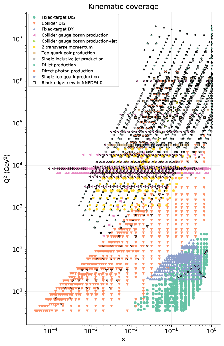
Figure 2.1: The kinematic coverage of the NNPDF4.0 dataset in the $(x,Q^{2})$ plane.

The complete information on experimental uncertainties, including the breakdown into different sources of systematic uncertainties and their correlations, is taken into account whenever available from the corresponding publications or from the HEPData repository [150]. No decorrelation models are used, except when explicitly recommended by the collaboration. This is the case of the single-inclusive jet cross-section measurement performed by ATLAS at $\sqrt{s}=8$ TeV [88]. Decorrelation models [151, 9, 152, 153, 154] were studied for the ATLAS jet measurements at $\sqrt{s}=7$ TeV [75] and for the ATLAS top pair measurements at $\sqrt{s}=8$ TeV [69]. However these are not considered in our default determination, but only in variant fits, see Sect. 8.7.

2.2 New data in NNPDF4.0

We now discuss in detail the new datasets considered in NNPDF4.0. These are indicated with an asterisk in Tables 2.1-2.5. The data are presented by process, with the processes already considered in NNPDF3.1 addressed first.

2.2.1 Deep-inelastic scattering

We include the combined H1 and ZEUS measurements of reduced electron-proton NC DIS cross-sections for the production of open charm and bottom quarks [145]. These measurements extend the previous combination of open charm production cross-sections [41] and supersede the separate H1 [42] and ZEUS [43] datasets for the structure function $F_{2}^{b}$ that were included in NNPDF3.1. As for the other DIS measurements included in the NNPDF4.0 dataset, they are analyzed in the FONLL scheme [25, 134, 135] within fixed order perturbative accuracy (i.e. not including resummation).

We also consider the measurements of the ratio $\mathcal{R}_{\mu\mu}$ of dimuon to inclusive neutrino-nucleus CC DIS cross-sections performed by the NOMAD experiment [111]. These measurements are presented alternatively as a function of the neutrino beam energy $E_{\nu}$, of the momentum fraction $x$, or of the final state invariant mass $W$. Because experimental correlations are not provided among the three distributions, they cannot be included in the fit at the same time. We therefore select only one of them, namely the measurement as a function of the neutrino beam energy, the only variable among the three that is directly measured by the experiment. This choice is based on the previous study [10], carried out in the context of a variant of the NNPDF3.1 determination, in which it was shown that the three distributions have a similar impact in the fit.

The treatment of this dataset in NNPDF4.0 closely follows Ref. [10]. Specifically we incorporate the recently computed NNLO charm-quark massive corrections [140, 139] by means of a $K$-factor (see Sect. 2.2.2 in [10]). The NOMAD data are not included in our default determination, however we assess its impact on the NNLO PDFs by means of Bayesian reweighting [155, 156]. The reason for this choice is dictated by the fact that the observable is integrated over $Q$ and $x$ (see e.g. Eq. (2.1) in Ref. [10]), which complicates the generation of fast interpolation tables in the APFELgrid format.

2.2.2 Jet production in deep-inelastic scattering

We consider a selection of DIS single-inclusive jet (1j) and dijet production (2j) cross-sections measured by ZEUS [112, 113, 114] in the high-$Q$ (HQ) region and by H1-HeraII [115, 116] in the HQ and low-$Q$ (LQ) regions. Specifically we consider cross-sections double differential in $Q^{2}$ and in the transverse momentum of the jet or of the jet pair, listed in Table 2.2. Experimental correlations between single-inclusive jet and dijet measurements, which are available only for H1, are taken into account. These allow us to include single-inclusive jet and dijet datasets simultaneously. Additional available measurements, in particular from H1-HeraI [157, 158], are left for future studies. Likewise, variants of the H1-HeraII measurements [115, 116], in which cross-sections are normalized to the inclusive NC cross-section integrated over the width of each $Q^{2}$ bin, are not yet considered. These normalized cross-sections might benefit from cancellations of systematic uncertainties and uncertainty correlation with HERA inclusive DIS measurements.

Theoretical predictions for the ZEUS and H1-HeraII datasets are obtained using fast interpolation grids precomputed with NNLOjet. These incorporate the recently determined NNLO QCD corrections [159]. Multiplicative hadronization correction factors, as provided in the experimental analyses, are included throughout. Because this theoretical input has become available only very recently, the ZEUS and H1-HeraII datasets are not included in our default determination, but only in a variant NNLO set by means of Bayesian reweighting, see Sect. 7.3.5.

2.2.3 Fixed-target Drell-Yan production

We consider the new measurement recently performed by the SeaQuest experiment at Fermilab [117] for production of a $Z$ boson decaying into muon pairs. Like the previous NuSea measurement [47], which was included in the NNPDF3.1 dataset, the SeaQuest experiment measures the ratio of the scattering cross-section of a proton beam off a deuterium target to the cross-section off a proton target. The measurement is double differential in the partonic momentum fractions of the struck partons. The SeaQuest data extend the NuSea data to larger values of $x$, $0.15\lesssim x\lesssim 0.40$, with the aim of constraining the antiquark asymmetry in this region [47]. Theoretical predictions are computed by taking into account acceptance corrections, according to Eq. (10) in Ref. [117]. Fast interpolation tables accurate to NLO are generated with APFEL; these are then supplemented with a NNLO $K$-factor computed with a version of Vrap [160] that we modified to account for the isoscalarity of the deuteron target. Nuclear effects are taken into account by means of the procedure discussed in Ref. [19] and further summarized in Sect. 2.3.

2.2.4 Inclusive collider electroweak gauge boson production

The new datasets we consider for inclusive $W$ and $Z$ boson production and decay are from the ATLAS and LHCb experiments.

We include the ATLAS measurements of the $W$ and $Z$ differential cross-section at $\sqrt{s}=7$ TeV [54] in the central and forward rapidity regions. As mentioned above, these data were already included in NNPDF3.1, but only the subset corresponding to the central region. The measurements cover, respectively, the pseudo-rapidity range $|\eta_{\ell}|<2.5$ (for $W$ bosons) and the rapidity range of the lepton pair $|y_{\ell\ell}|<3.6$ (for the $Z$ boson). In the latter case, the invariant mass of the lepton pair is $46\leq m_{\ell\ell}\leq 150$ GeV. The measurements correspond to an integrated luminosity of 4.6 fb^-1. We consider the combination of measurements in the electron and muon decays.

We consider the ATLAS measurements of the double and triple differential DY lepton pair production cross-section at $\sqrt{s}=8$ TeV [79, 80]. The differential variables are the invariant mass and rapidity of the lepton pair, $m_{\ell\ell}$ and $y_{\ell\ell}$, and, in addition to these for the latter case, the cosine of the Collins-Soper angle $\cos\theta^{*}$. The measurements cover two separate invariant mass ranges, respectively $116\leq m_{\ell\ell}\leq 1500$ GeV and $46\leq m_{\ell\ell}\leq 200$ GeV, in the same central rapidity range $|y_{\ell\ell}|<2.4$. The same data sample corresponding to an integrated luminosity of 20.2 fb^-1 is used in the two cases, which therefore overlap in the interval $116\leq m_{\ell\ell}\leq 200$ GeV. The two analyses are consistent in this region, however because the one in [79] is optimized to high invariant masses, we remove the overlapping bins from the dataset in [80]. In both cases we consider the measurements in which the electron and muon decay channels have been combined; for the triple differential distribution, we consider the measurement integrated over $\cos\theta^{*}$ in order to reduce sensitivity to the value of the Weinberg angle $\sin^{2}\theta_{W}$.

We include the ATLAS measurement of the $W$ production cross-section and decay at $\sqrt{s}=8$ TeV [81]. The data are differential in the pseudo-rapidity of the decay muon $\eta_{\mu}$, which is accessed in the central pseudo-rapidity range $|\eta_{\mu}|<2.4$ by analyzing a data sample corresponding to an integrated luminosity of 20.2 fb^-1. As for the companion ATLAS measurement at $\sqrt{s}=7$ TeV [54], we consider the separate $W^{+}$ and $W^{-}$ differential distributions rather than their asymmetry.

We consider the ATLAS measurement of the total $W$ and $Z$ cross-section and decay into leptons at $\sqrt{s}=13$ TeV [83]. The measurement corresponds to an integrated luminosity of 81 pb^-1.

We include the LHCb measurement of the $W$ cross-section at $\sqrt{s}=8$ TeV [82]. The data are differential in the pseudo-rapidity of the decay electron $\eta_{e}$, which is accessed in the forward range $2.00<|\eta_{e}|<4.25$. The data sample corresponds to an integrated luminosity of 2 fb^-1. In this case, we cannot consider the separate $W^{+}$ and $W^{-}$ differential distributions, because we find that the correlated experimental uncertainties lead to a covariance matrix that is not positive definite. Therefore, in this case we make use of the asymmetry measurement, which is not affected by this problem since most of the correlations cancel out.

Finally, we include the LHCb measurement of the $Z$ cross-section at $\sqrt{s}=13$ TeV [84]. The data are differential in the $Z$ boson rapidity $y_{Z}$ [84], with $2.00<|y_{Z}|<4.50$, and it covers the $Z$-peak lepton pair invariant mass range $60\leq m_{\ell\ell}\leq 120$ GeV. The data sample corresponds to an integrated luminosity of 294 pb^-1. We include separately the datasets in the dimuon and dielectron decay channels.

These datasets, specifically from ATLAS, are particularly precise, with systematic uncertainties of the order of percent or less and even smaller statistical uncertainties. They are dominated by the luminosity uncertainty, which is of the order of 1.9-2.1% (1.2-3.9%) for ATLAS (LHCb) respectively at $\sqrt{s}=8$ TeV and at $\sqrt{s}=13$ TeV.

Theoretical predictions are computed at NLO with MCFM (v6.8) [120, 121, 122] and are benchmarked against those obtained with mg5_aMC (v3.1) [124, 125]. The NNLO $K$-factor is computed with FEWZ (v3.1) [161, 162, 163] for all the datasets excepting those of [80, 81], for which DYNNLO [164, 165] is used instead. We benchmarked these calculations against MCFM (v9.0) [166], and found the relative difference between different computations to be negligible in comparison to the data uncertainties. The renormalization and factorization scales are set equal to the mass of the gauge boson, for total cross-sections and for cross-sections differential in rapidity or pseudorapidity variables, or to the central value of the corresponding invariant mass bin, for cross-sections that are also differential in the invariant mass of the lepton pair.

2.2.5 Gauge boson production with additional jets

On top of inclusive gauge boson production, we consider more exclusive measurements in which a $W$ boson is produced in association with $N_{\rm jets}$ jets of light quarks, or with a single jet of charm quarks.

Specifically, we include the ATLAS data for $W$ production with $N_{\rm jets}\geq 1$ [95] at $\sqrt{s}=8$ TeV. The measurement corresponds to an integrated luminosity of 20.2 fb^-1. We select the distribution differential in the transverse momentum of the $W$ boson, $p_{T}^{W}$, which covers the range $0\leq p_{T}^{W}\leq 800$ GeV. Theoretical predictions are determined as in the ATLAS study of [167]: at NLO, fast interpolation grids are generated with MCFM; at NNLO, QCD corrections are implemented by means of $K$-factors determined with the $N_{\rm jetti}$ program [168, 169]. The factorization and renormalization scales are set equal to the mass of the $W$ boson.

We further include the ATLAS [85] and CMS [86] data for production of $W$ with a charm jet, at $\sqrt{s}=7$ TeV and $\sqrt{s}=13$ TeV, respectively. The two measurements correspond to integrated luminosities of 4.6 fb^-1 and 35.7 fb^-1. In both cases, we utilize the cross-sections differential in the pseudo-rapidity of the decay lepton $\eta_{\ell}$, which is accessed in the range $|\eta_{\ell}|<2.5$ for ATLAS and $|\eta_{\ell}|<2.4$ for CMS. In the case of ATLAS, separate distributions for the production of positively and negatively charged bosons are provided; in the case of CMS, only the distribution for the sum of the two is available. Theoretical predictions are computed at NLO with MCFM; NNLO QCD corrections have been computed very recently [87], although in a format that does not allow for their ready implementation. These datasets are therefore not included in the determination of NNLO PDFs. The factorization and renormalization scales are set equal to the mass of the $W$ boson.

All the measurements discussed in this section have been included in a PDF determination, in a specific study based on NNPDF3.1 [10].

2.2.6 Top pair production

We consider several new datasets for top pair production at the LHC. At $\sqrt{s}=8$ TeV, we include the ATLAS normalized differential cross-section [91] and the CMS normalized double differential cross-section [92], both of which are measured in the dilepton channel. Companion measurements in the lepton+jets channel [69, 72] were already part of NNPDF3.1. These measurements correspond respectively to an integrated luminosity of 20.2 fb^-1 and 19.7 fb^-1. At $\sqrt{s}=8$ TeV, we include the ATLAS total cross-section [136] and the CMS absolute differential distributions in the lepton+jets channel [93] and in the dilepton channel [94]. The ATLAS measurement is based on the full Run II sample, corresponding to an integrated luminosity of 139 fb^-1 and replaces the corresponding measurement, determined from a partial luminosity [68], included in NNPDF3.1; the CMS measurements are for an integrated luminosity of 35.8 fb^-1.

Various differential distributions are available for each of these measurements. Because correlations between different distributions are not available, only one distribution at a time can be included. Rapidity distributions are generally affected by small higher order corrections [170], hence we chose the rapidity of the top quark, when available, as our preferred observable, and otherwise, the rapidity of the top pair. Specifically, we select the distributions differential in the rapidity of the top pair in the case of [91], the double-differential distribution in the rapidity of the top quark and the invariant mass of the top pair in the case of [92] and in the rapidity of the top quark in the case of [93, 94]. We have explicitly verified that the choice of any other distributions does not alter the results. The kinematic coverage of the distributions that we included is shown in Table 2.5.

Theoretical predictions are computed at NLO with mg5_aMC (v2.6.6) [125]; NNLO QCD corrections are determined from publicly available FastNLO tables [171, 172] for differential distributions and from top++ [173] for the total cross-section. The renormalization and factorization scales are set as in NNPDF3.1, see Sect. 2.7 in [5] for details.

2.2.7 Single-inclusive and dijet production

In NNPDF4.0, following the study of Ref. [9], we consider both single-inclusive jets (as in previous NNPDF determinations) and dijets, that have several desirable theoretical features [137].

For single-inclusive jet production, we include the ATLAS [88] and CMS [89] measurements at $\sqrt{s}=8$ TeV. They correspond to integrated luminosities of 20.2 fb^-1 and 19.7 ^-1, respectively. In both cases the measurements are provided for the cross-section differential in the transverse momentum, $p_{T}^{\rm jet}$, and of the rapidity, $y^{\rm jet}$, of the jet. The data cover the range $70\leq p_{T}^{\rm jet}\leq 2.5$ TeV and $|y^{\rm jet}|\leq 3.0$. Theoretical predictions are computed at NLO with NLOJet++ (v4.1.3) [126] and benchmarked against the independent computation presented in [174]. NNLO QCD corrections are incorporated by means of the $K$-factor computed in the same publication. The factorization and renormalization scales are set equal to the optimal scale choice recommended in Ref. [137], namely, the scalar sum of the transverse momenta of all partons in the event.

For dijet production we consider the ATLAS [148] and CMS [76] measurements at $\sqrt{s}=7$ TeV and the CMS measurement [149] at $\sqrt{s}=8$ TeV. They correspond to integrated luminosities of 4.5 fb^-1 (at 7 TeV) and of 19.7 fb^-1 (at 8 TeV). For ATLAS, the cross-section is double differential in the dijet invariant mass $m_{jj}$ and in the absolute difference of the rapidities of the two jets $y^{*}$. The corresponding ranges are $260\leq m_{jj}\leq 4.27$ TeV and $0.0\leq y^{*}\leq 3.0$. For CMS, the cross-section is double differential in $m_{jj}$ and in the maximum absolute rapidity of the two jets $|y_{\rm max}|$ (at 7 TeV) and triple differential in the average transverse momentum of the jet pair $p_{T,{\rm avg}}$, the dijet boost $y_{b}$, and $y^{*}$ (at 8 TeV). The corresponding ranges are $133\leq p_{T,{\rm avg}}\leq 1.78$ TeV and $0.0\leq y_{b},y^{*}\leq 3.0$. As in the case of single-inclusive jets, theoretical predictions are computed at NLO with NLOJet++ and are benchmarked against the independent computation of Ref. [174]. This computation is also used to determine the NNLO QCD corrections, implemented as $K$-factors. The renormalization and factorization scale used in the computation are set to the invariant mass of the dijet system, again following the recommendation of Ref. [137].

Single-inclusive jet and dijet observables cannot be simultaneously included because full knowledge of the experimental correlations between them is not available. The selection of the optimal set of jet observables will be performed and discussed in Sect. 4, in the context of the final dataset selection.

2.2.8 Inclusive isolated-photon production

Isolated photon production was not included in previous NNPDF releases and is included in NNPDF4.0 for the first time. We specifically consider the ATLAS measurements at $\sqrt{s}=8$ TeV [102] and $\sqrt{s}=13$ TeV [175]. They correspond to integrated luminosities of 20.2 fb^-1 and 3.2 fb^-1, respectively. The measurements are provided for the cross-section differential in the photon transverse energy $E_{T}^{\gamma}$ in different bins of the photon pseudorapidity $\eta_{\gamma}$. The accessed ranges are, in both cases, $E_{T}^{\gamma}<1500$ GeV and $|\eta_{\gamma}|<2.37$. Theoretical predictions are computed at NLO with MCFM and benchmarked against the independent computation presented in [176]. The smooth cone isolation criterion [177] is adopted accordingly, with the parameter values determined in [178]. NNLO QCD corrections are incorporated by means of the $K$-factors computed in [176]; $K$-factors are also used to incorporate corrections due to resummation of the electroweak Sudakov logarithms at leading-logarithmic accuracy, according to the procedure presented in [179, 180]. The factorization and renormalization scales are set equal to the central value of $E_{T}^{\gamma}$ for each bin. The impact of the measurements presented above on a PDF determination was studied in [7] in the context of a variant of the NNPDF3.1 fit. These data were found to be generally well described, except in the most forward rapidity region, and to have a mild impact on the gluon PDF at intermediate values of $x$.

2.2.9 Single top production

Another process included for the first time in an NNPDF release is $t$-channel single top production. We consider the ATLAS [96, 98, 100] and CMS [97, 99, 101] measurements at $\sqrt{s}=7$, 8 and 13 TeV that correspond, for ATLAS (CMS), to integrated luminosities of 4.59, 20.2 and 3.2 fb^-1 (2.73, 19.7 and 2.2 fb^-1), respectively. In the case of ATLAS, we consider the ratio of the top to antitop inclusive cross-sections at 7 and 13 TeV and the distributions differential in the top or antitop rapidity $y_{t,\bar{t}}$ at 7 and 8 TeV normalized to the corresponding total cross-section. The rapidity ranges are $|y_{t,\bar{t}}|<3.0$ and $|y_{t,\bar{t}}|<2.2$ at $\sqrt{s}=7$ and 8 TeV, respectively. In the case of CMS, we consider the sum of the top and antitop inclusive cross-sections at 7 TeV and the ratio of the top to antitop inclusive cross-sections at 8 and 13 TeV. Theoretical predictions are computed in the five-flavor scheme. At NLO the calculation is performed with mg5_aMC (v2.6.6) [125]; NNLO corrections are incorporated by means of the $K$-factors determined in [181, 182]. The renormalization and factorization scales are set equal to the top mass.

The measurements presented above were extensively studied in the context of a variant of the NNPDF3.1 fit in [8]. The choice of observables included for PDF determinations is based on the results of that reference. In particular, distributions differential in the transverse momentum of the top quark or antiquark are also provided by the experimental collaborations. However, their inclusion would result in a double counting, given that experimental correlations across uncertainties for different distributions are not provided. In [8] these measurements were found to have a mild impact on the up and down PDFs at $x\gtrsim 0.1$.

Single top $t$-channel production is in principle also sensitive to the theoretical details of the matching schemes and, in the five-flavor scheme, to the bottom PDF. Here we determine the bottom PDF using perturbative matching conditions, but it could in principle be parametrized independently, like the charm PDF. However, while this may become relevant in the future, it does not seem necessary at present given the precision and kinematic coverage of the existing data.

2.3 Treatment of nuclear corrections

The NNPDF4.0 dataset, like its predecessors, includes a significant amount of data involving deuterium or heavy nuclear targets, both for deep inelastic and hadronic processes. These are summarized in Table 2.6, where we also report the corresponding reference, the number of data points in the NLO and NNLO baseline fits, and the species of the nuclear target. Overall, 1416 and 1417 data points come from nuclear measurements in the NLO and NNLO fits respectively, which amount to about 30% of the full dataset. All of these datasets but SeaQuest [117] were already included in the previous NNPDF3.1 determination [5].

Dataset	Ref.	$N_{\rm dat}$	Target	Dataset	Ref.	$N_{\rm dat}$	Target
NMC $F_{2}^{d}/F_{2}^{p}$	[33]	121/121	$p$, $d$	CHORUS $\sigma_{CC}^{\nu}$	[37]	416/416	${}^{208}_{\ 82}$Pb
SLAC $F_{2}^{d}$	[35]	34/34	$d$	CHORUS $\sigma_{CC}^{\bar{\nu}}$	[37]	416/416	${}^{208}_{\ 82}$Pb
BCDMS $F_{2}^{d}$	[36]	248/248	$d$	NuTeV $\sigma_{CC}^{\nu}$ (dimuon)	[38, 39]	39/39	${}^{56}_{26}$Fe
E866 $\sigma^{d}/2\sigma^{p}$ (NuSea)	[47]	15/15	$p$, $d$	NuTeV $\sigma_{CC}^{\bar{\nu}}$ (dimuon)	[38, 39]	36/37	${}^{56}_{26}$Fe
E906 $\sigma^{d}/2\sigma^{p}$ (seaQuest)	[117]	6/6	$p$, $d$	E605 $\sigma^{p}$	[45]	85/85	${}^{64}_{32}$Cu
				EMC $F_{2}^{c}$	[44]	—/16	${}^{56}_{26}$Fe

Table 2.6: The nuclear datasets in NNPDF4.0 involving deuterium targets (left) or heavier nuclear targets (right) and corresponding targets; $N_{\rm dat}$ denotes the number of data points included in the NLO/NNLO fits. Note that the EMC $F_{2}^{c}$ dataset is not included in the default NNPDF4.0 PDF set.

The inclusion of nuclear data in a fit of proton PDFs requires accounting for changes in the PDFs induced by the nuclear medium. The impact of such changes was studied by us in [183, 14] and found to be subdominant in comparison to the PDF uncertainty at that time. Specifically, it was shown (see Sect. 4.11 in [5]) that, upon removing data with nuclear targets from the dataset, the precision of up, down and strange quark and anti-quark PDFs deteriorated by an amount larger than the size of the effect of the nuclear corrections estimated on the basis of models. Nuclear corrections were consequently not included in the NNPDF3.1 determination.

In NNPDF4.0 we revisit this state of affairs, motivated by the significant reduction of the PDF uncertainty in comparison to NNPDF3.1, which suggests that nuclear effects can no longer be neglected. We now account for nuclear effects by viewing them as a theoretical uncertainty. The way this is determined and included follows the methodology developed in [18, 19], to which we refer for details. The basic idea is to determine the uncertainty from the difference between the values of observables computed with the proton and nuclear PDFs, with each different determination of the nuclear PDF taken as an independent nuisance parameter. This can then be used to compute a theoretical covariance matrix, that can be added to the experimental covariance matrix.

In order to apply this methodology an underlying set of nuclear PDFs is needed for the computation of the shifts. Heavy nuclear and deuteron corrections are treated separately because of the substantial difference in the observed size and expected origin of the nuclear effects. For heavier nuclei (Fe, Cu and Pb targets) we will use the nNNPDF2.0 nuclear PDFs [20]. For deuterium, we use the self-consistent procedure described in [19], whereby the proton and deuteron PDFs are determined simultaneously, each including the uncertainties on the other. This procedure thus requires in turn the use of a PDF determination without deuterium corrections in order to initiate the self-consistent iteration. Here we will apply it by starting with the NNPDF4.0 determination itself. The deuterium PDF determined by this procedure will be described in Sect. 8.6 below.

While nuclear effects will be included as an extra uncertainty in the default NNPDF4.0 determination, we will also discuss for comparison PDFs obtained by neglecting nuclear effects altogether, or by using the nuclear corrections computed as discussed above as a correction to the data and not just as an additional uncertainty, again following the methodology of Refs. [18, 19]. These alternative treatments of nuclear effects will be compared and discussed in Sect. 8.6 below and provide the motivation for including nuclear uncertainties without a correction in the default PDF determination.

3 Fitting methodology

As discussed in the introduction, NNPDF4.0 is the first PDF set to be based on a methodology fully selected through a machine learning algorithm. This means that, whereas the basic structure of the NNPDF4.0 methodology is the same as in previous NNPDF releases, specifically the use of a Monte Carlo representation of PDF uncertainties and correlations, and the use of neural networks as basic interpolating functions [14, 5], all the details of the implementation, such as the choice of neural network architecture and the minimization algorithm, are now selected through an automated hyperoptimization procedure. This is possible thanks to an extensive rewriting and reorganization of the NNPDF framework. Furthermore, some theory constraints built into the PDF parametrization are implemented for the first time in NNPDF4.0. Also for the first time we consider PDF determinations performed with different choices of parametrization basis.

In Sect. 3.1 we start by discussing the PDF parametrization and choice of basis and the way they implement theoretical constraints. In Sect. 3.2 we then present the new NNPDF fitting framework, which is the basis of the hyperoptimization procedure. The hyperoptimization in turn is discussed in Sect. 3.3, along with its output, which defines the baseline NNPDF4.0 methodology. We conclude in Sect. 3.4 with quantitative benchmarks assessing both the efficiency and speed of this final methodology compared to the methodology used for NNPDF3.1.

3.1 PDF parametrization and theoretical constraints

We now turn to the general structure of the PDF parametrization, and the theory constraints that are imposed upon it: specifically sum rules, positivity and integrability.

3.1.1 Parametrization bases

A PDF analysis requires a choice of basis, namely a set of linearly independent PDF flavor combinations that are parametrized at the input evolution scale $Q_{0}$. In the NNPDF approach, this corresponds to choosing which are the PDF combinations whose value is the output of a neural network. Optimal results should in principle be independent of this specific choice of basis. Previous NNPDF releases adopted the so-called evolution basis, in which the basis PDFs are chosen as the singlet quark $\Sigma$ and gluon $g$ that mix upon QCD evolution, and valence $V_{i}$ and nonsinglet sea $T_{i}$ combinations that are eigenstates of evolution, namely

$$\Sigma =u+\bar{u}+d+\bar{d}+s+\bar{s}+2c\,,$$

$$T_{3} =\left(u+\bar{u}\right)-\left(d+\bar{d}\right)\,,$$

$$T_{8} =\left(u+\bar{u}+d+\bar{d}\right)-2\left(s+\bar{s}\right)\,$$ (3.1)

$$V =\left(u-\bar{u}\right)+\left(d-\bar{d}\right)+\left(s-\bar{s}\right)\,,$$

$$V_{3} =\left(u-\bar{u}\right)-\left(d-\bar{d}\right)\,,$$

$$V_{8} =\left(u-\bar{u}+d-\bar{d}\right)-2\left(s-\bar{s}\right)\,.$$

In NNPDF3.1, this set of linearly independent flavor combinations was supplemented by an independently parametrized total charm PDF $c+\bar{c}$, with the charm asymmetry $c-\bar{c}$ assumed to vanish at scale $Q_{0}$. Here we will instead supplement the basis Eq. (3.1) with a further nonsinglet combination, namely

$$T_{15}=\left(u+\bar{u}+d+\bar{d}+s+\bar{s}\right)-3\left(c+\bar{c}\right)$$ (3.2)

still assuming $c-\bar{c}=0$ at the parametrization scale. At NNLO a small charm asymmetry is then generated by perturbative evolution. The union of Eqs. (3.1-3.2) will be referred to as the evolution basis henceforth.

We will also consider PDF determnations carried out in the flavor basis, in which the PDFs that are parametrized are

$$\tilde{f}_{k}=\{u,\,\bar{u},\,d,\bar{d},\,s,\,\bar{s},\,c,\,g\},$$ (3.3)

related to their evolution basis counterparts

$${f}_{k}=\{V,\,V_{3},\,V_{8},\,T_{3},\,T_{8},\,T_{15},\,\Sigma,\,g\},$$ (3.4)

by means of Eqns. (3.1-3.2).

The evolution and flavor bases each have advantages and disadvantages. For instance, if one chooses a factorization scheme in which PDFs are non-negative [21], positivity is easier to implement in the flavor basis. On the other hand, the integrability of the valence distributions $V,V_{3},V_{8}$, as required by the valence sum rules, is simpler in the evolution basis. In this work, we take the evolution basis as our standard choice, however we will explicitly check basis independence, by verifying that equivalent results are obtained in the data region if the flavor basis is adopted instead, see Sect. 8.4 below.

The output of the neural network is supplemented by a preprocessing factor and by normalization constants. The relation between the PDFs and the neural network output is

$$xf_{k}\left(x,Q_{0};{\boldsymbol{\theta}}\right)=A_{k}\,x^{1-\alpha_{k}}(1-x)^{\beta_{k}}{\rm NN}_{k}(x;{\boldsymbol{\theta}})\,,\quad k=1,\ldots,8\,,$$ (3.5)

where $k$ runs over the elements of the PDF basis, ${\rm NN}_{k}(x;{\boldsymbol{\theta}})$ is the $k$-th output of a neural network, and ${\boldsymbol{\theta}}$ collectively indicates the full set of neural network parameters. The preprocessing function has the purpose of speeding up the training of the neural net. In order to make sure that it does not bias the result, the exponents $\alpha_{k}$ and $\beta_{k}$ are varied in a range that is determined iteratively in a self-consistent manner as described in [14], supplemented by a further integrability constraint, to be discussed in Sec. 3.1.4. The independence of result of the choice of preprocessing ranges has been recently validated in Ref. [184], where it is shown that results otained here can be obtained by a suitable rescaling on the neural network input that avoids preprocessing altogether. The normalization constants $A_{k}$ are constrained by the valence and momentum sum rules, also to be discussed below, in Sec. 3.1.2.

When using the flavor basis, the small-$x$ preprocessing is removed from Eq. (3.5), i.e. $\alpha_{k}=1$ for all $k$. This is because standard Regge theory arguments (see e.g. [185]) imply that the singlet and nonsinglet have a different small $x$ behavior, and in particular the nonsinglet has a finite first moment, while the singlet first moment diverges. This means that the small-$x$ behavior of flavor-basis PDFs is the linear combination of a leading singlet small-$x$ growth and a subleading nonsinglet power behavior characterized by a different exponent. Hence, factoring out a common preprocessing exponent is not advantageous in this case.

3.1.2 Sum rules

Irrespectively of the choice of fitting basis, PDFs should satisfy both the momentum sum rule

$$\int_{0}^{1}dx\,x\left(g\left(x,Q\right)+\Sigma\left(x,Q\right)\right)=1\,,$$ (3.6)

and the three valence sum rules,

$$\int_{0}^{1}dx\,\left(u(x,Q)-\bar{u}(x,Q)\right) = 2\,,$$

$$\int_{0}^{1}dx\,\left(d(x,Q)-\bar{d}(x,Q)\right) = 1\,,$$ (3.7)

$$\int_{0}^{1}dx\,\left(s(x,Q)-\bar{s}(x,Q)\right) = 0\,,$$

for all values of $Q$. Provided these sum rules are imposed at the initial parametrization scale, $Q_{0}$, perturbative QCD ensures that they will hold for any other value $Q\neq Q_{0}$. When transformed to the evolution basis, Eq. (3.8), the valence sum rules read

$$\int_{0}^{1}dx\,V\left(x,Q\right)=\int_{0}^{1}dx\,V_{8}\left(x,Q\right)=3\,,\quad\int_{0}^{1}dx\,V_{3}\left(x,Q\right)=1\,.$$ (3.8)

We have then four equations that fix four of the normalization constants $A_{k}$, namely $A_{V}$, $A_{V_{8}}$,$A_{V_{3}}$ and $A_{g}$.

In the present analysis we always impose the sum rules in the evolution basis. This means that when performing a fit in the flavor basis, we express the evolution basis PDFs $f_{k}$ Eq. (3.4) in terms of the flavor basis PDFs $\tilde{f}_{k}$ Eq. (3.3) through a transformation matrix $R_{kk^{\prime}}$:

$$xf_{k}\left(x,Q_{0};{\boldsymbol{\theta}}\right)=A_{k}\sum_{k^{\prime}}R_{kk^{\prime}}\,x\tilde{f}_{k^{\prime}}\left(x,Q_{0};{\boldsymbol{\theta}}\right),$$ (3.9)

and then impose Eqs. (3.6,3.8).

The integrals in Eqs.(3.6,3.8) are evaluated between $x_{\rm min}=10^{-9}$ and $x_{\rm max}=1$. Each time the neural network parameters ${\boldsymbol{\theta}}$ are modified by the minimization algorithm, using an adaptative strategy that achieves a relative precision of $\mathcal{O}\left(10^{-5}\right)$ across the whole range of $x$.

3.1.3 Positivity of PDFs and physical observables

Hadron-level cross-sections are non-negative quantities, because they are probability distributions. However, PDFs beyond LO are not probabilities, and thus they may be negative. The reason is that, beyond LO, PDFs include a collinear subtraction which is necessary in order for the partonic cross-sections to be finite. Whether they remain positive or not then depends on the form of the subtraction, i.e. on the factorization scheme. Consequently, in previous NNPDF determinations, in order to exclude unphysical PDFs, we imposed positivity of a number of cross-sections, by means of Lagrange multipliers which penalize PDF configurations leading to negative physical observables. Specifically, we imposed positivity of the $F_{2}^{u}$, $F_{2}^{d}$, $F_{2}^{s}$, and $F_{L}$ structure functions and of the flavor-diagonal Drell-Yan rapidity distributions $\sigma_{{\rm DY},u\bar{u}}$, $\sigma_{{\rm DY},d\bar{d}}$, $\sigma_{{\rm DY},s\bar{s}}$. However, since this set of positivity observables is not exhaustive, in some extreme kinematic regions physical observables (e.g. very high-mass $W^{\prime}$ production) could still become negative within uncertainties.

It was recently shown in Ref. [21] that PDFs for individual quark flavors and the gluon in the $\overline{\rm MS}$ factorization scheme are non-negative. We thus now also impose this positivity condition along with the constraint of positivity of physical cross-sections discussed above. Indeed, note that the positivity of $\overline{\rm MS}$ PDFs is neither necessary nor sufficient in order to ensure cross-section positivity [21]: they are independent (though of course related) constraints that limit the space of acceptable PDFs.

We impose positivity of the gluon and of the up, down and strange quark and antiquark PDFs. The charm PDF is also positive in the $n_{f}=3$ scheme, but it needs not be positive in the $n_{f}=4$ scheme because perturbative matching conditions neglect the quark mass and this generally spoils positivity for a massive quark PDF [21]. We do, however, add a positivity constraint for the charm structure function $F_{2}^{c}$, similar to the ones for other structure functions of individual flavors. Note that this constraint was not included in NNPDF3.1, though it was included in a more recent study based on NNPDF3.1 dataset and methodology [10], where it was found to have a significant impact on the strange PDF.

In the same manner as for the cross-sections, PDF positivity is implemented by means of Lagrange multipliers. Specifically, for each flavor basis PDF $\tilde{f}_{k}$ Eq. (3.3), one adds a contribution to the total cost function used for the neural network training given by

$$\chi^{2}_{\rm tot}\to\chi^{2}_{\rm tot}+\sum_{k=1}^{8}\Lambda_{k}\,\sum_{i=1}^{n_{i}}\,\text{Elu}_{\alpha}\left(-\tilde{f}_{k}\left(x_{i},Q^{2}\right)\right)\,,$$ (3.10)

with $Q^{2}=5\,\text{GeV}^{2}$ and with the $n_{i}$ values $x_{i}$ given by 10 points logarithmically spaced between $5\cdot 10^{-7}$ and $10^{-1}$ and 10 points linearly spaced between $0.1$ and $0.9$. The Elu function is given by

$$\text{Elu}_{\alpha}\left(t\right)=\begin{cases}t\,\,\,\,\,\,\,\,\,\,\,\,\,\,\,\,\,\,\,\,\,\,\,\,\,\,\,\,\,\,\,\text{if}\,\,\,\,t>0\\ \alpha\left(e^{t}-1\right)\,\,\,\,\,\,\,\text{if}\,\,\,\,t<0\end{cases}\,,$$ (3.11)

with the parameter $\alpha=10^{-7}$. Eq. (3.10) indicates that negative PDFs receive a penalty which is proportional both to the corresponding Lagrange multipliers $\Lambda_{k}$ and to the absolute magnitude of the PDF itself, and therefore these configurations will be strongly disfavored during the minimization. The Lagrange multiplier increases exponentially during the minimization, with a maximum value $\Lambda_{k}^{\rm max}$ attained when the maximum training length is reached. We choose $\Lambda_{k}^{\rm max}=10^{10}$ for the three Drell-Yan observables, and $\Lambda_{k}^{\rm max}=10^{6}$ for all the other positivity observables. These values are chosen in such a way that the constraint is enforced with sufficient accuracy in all cases. The starting values of the Lagrange multipliers and the maximum training length instead are determined as part of the hyperoptimization procedure described in Sect. 3.3 below.

When performing fits in the evolution basis, this PDF positivity constraint is applied after performing the inverse transformation to Eq. (3.9) in order to express the flavor basis PDFs $\tilde{f}_{k}$ Eq. (3.3) in terms of their evolution basis counterparts $f_{k}$.

3.1.4 PDF integrability

The small-$x$ behavior of the PDFs is constrained by integrability requirements. First, the gluon and singlet PDFs must satisfy the momentum sum rule, Eq. (3.6), which implies that

$$\lim_{x\rightarrow 0}\,x^{2}f_{k}(x,Q)=0\,,\quad\forall~{}Q\,,\qquad f_{k}=g,\,\Sigma\,,$$ (3.12)

while the valence sum rules, Eq. (3.8), constrain the small-$x$ behavior of the valence distributions,

$$\lim_{x\rightarrow 0}\,xf_{k}(x,Q)=0\,,\quad\forall~{}Q\,,\qquad f_{k}=V,\,V_{3}\,,V_{8}\,.$$ (3.13)

Furthermore, as mentioned, standard Regge theory arguments suggest that the first moments of the non-singlet combinations $T_{3}$ and $T_{8}$ are also finite, so for instance the Gottfried sum (which is proportional to the first moment of $T_{3}$) is finite. This implies that also for these two combinations one has

$$\lim_{x\rightarrow 0}\,xf_{k}(x,Q)=0\,,\quad\forall~{}Q\,,\qquad f_{k}=T_{3},\,T_{8}\,.$$ (3.14)

To ensure that these integrability requirements are satisfied, first of all we constrain the range of the small-$x$ preprocessing exponents $\alpha_{i}$ Eq. (3.5). We supplement the iterative determination of the exponents described in Ref. [14] with the constraints $\alpha_{k}<2$ for the singlet and gluon and $\alpha_{k}<1$ for the nonsinglet combinations $xV,\,xV_{3},\,xV_{8},\,xT_{3}$ and $xT_{8}$. Indeed if the preprocessing exponent were to violate these bounds, the neural net ${\rm NN}(x;{\boldsymbol{\theta}})$ in Eq. (3.5) would have to compensate this behavior in order for integrability to hold. Preprocessing would then be slowing the minimization rather than speeding it up. Note that, in the flavor basis, the small-$x$ preprocessing exponents are absent, so this requirement only applies to the evolution basis.

We observe that while Eq. (3.12) always turns out to be satisfied automatically when fitting to the experimental data, the additional constraints Eq. (3.13) and (3.14) can sometimes be violated by the fit, and thus must be imposed. This is also achieved through Lagrange multipliers. We include in the total cost function additional contributions of the form

$$\chi^{2}_{\rm tot}\to\chi^{2}_{\rm tot}+\sum_{k}\Lambda_{k}^{\rm(int)}\sum_{i=1}^{n_{i}}\,\left[xf_{k}\left(x_{\rm int}^{(i)},Q^{2}_{i}\right)\right]^{2}\,,$$ (3.15)

where $f_{k}=T_{3},T_{8}$ in the evolution basis while $f_{k}=V,V_{3},V_{8},T_{3},T_{8}$ in the flavor basis. The points $\{x_{\rm int}^{(i)}\}$ are a set of values in the small $x$ region, $Q^{2}_{i}$ is a suitable reference scale, and, like in the case of positivity, the Lagrange multipliers $\Lambda_{k}^{(\rm int)}$ grow exponentially during the minimization, with a maximum value $\Lambda_{k}^{(\rm int)}=100$ attained at maximum training length. We choose $Q_{i}^{2}=5$ GeV² and in the evolution basis $n_{i}=1$ and $x_{\rm int}^{(1)}=10^{-9}$, while in the flavor basis $n_{i}=3$ and $x_{\rm int}^{(i)}=10^{-9},\,10^{-8},\,10^{-7}$. As for the positivity multiplier, the starting values of the Lagrange multipliers (as well as the maximum training length) are hyperoptimization parameters.

Finally, we introduce a post-selection criterion, in order to discard replicas that fail to satisfy the integrability and retain a large value at small $x$ despite the Lagrange multiplier. It turns out that imposing

$$\sum_{i=1}^{n_{i}}\left|x_{\rm int}^{(i)}f_{k}\left(x_{\rm int}^{(i)}\right)\right|<{{1}\over{2}}\,,\qquad f_{k}=V,V_{3},V_{8},T_{3},T_{8}\,,$$ (3.16)

is enough to preserve integrability for all replicas. This is due to the fact that the function $xf(x)$ at its maximum is of order one, so the condition Eq. (3.16) ensures that at small $x$ it is decreasing. When determining PDF replicas, we have explicitly checked a posteriori that the numerical computation of the first moment yields a finite result for all PDF replicas.

3.2 Fitting framework

The machine learning approach to PDF determination that we will discuss shortly has been made possible by a complete restructuring of the NNPDF fitting framework. Further motivations for this are the need to deal with a particularly large dataset, and the goal of releasing the NNPDF code as open source, which imposes stringent requirements of quality and accessibility. The code was written in the Python programming language and has been documented and tested thoroughly. The original developments of our new fitting framework were presented in Ref. [11]. The main differences between the NNPDF3.1 and NNPDF4.0 codes are summarized in Tab. 3.1.

NNPDF3.1	NNPDF4.0
Genetic Algorithm optimizer	Gradient Descent optimization
one network per PDF	one network for all PDFs
sum rules imposed outside optimization	sum rules imposed during optimization
C++ monolithic codebase	Python object-ordiented codebase
fit parameters manually chosen (manual optimization)	fit parameters automatically chosen (hyperoptimization)
in-house ML framework	complete freddom in ML library choice (e.g. tensorflow)
private code	fully public open-source code

Table 3.1: Summary of the main differences between the NNPDF3.1 and the NNPDF4.0 code.

3.2.1 General structure

A schematic representation of the NNPDF4.0 fitting framework is displayed in Fig. 3.1. The fit requires three main inputs, which are managed by the NNPDF framework as discussed in Ref. [31]: first, theoretical calculations of physical processes, which are encoded in precomputed tables (FK-tables, see below) possibly supplemented by QCD and EW $K$-factors. Second, experimental data provided in a common format, including fully correlated uncertainties encoded in a covariance matrix (possibly also including theoretical uncertainties). Third, hyperparameter settings that determine the particular fitting methodology adopted, determined through a hyperoptimization procedure as discussed below. The neural network optimization algorithm, with settings determined by the hyperparameters, finds the best fit of predictions to data by minimizing a figure of merit whose computation is illustrated in Fig. 3.2. Following a post-fit selection, where outliers with insufficient quality are discarded, the final PDFs are stored in LHAPDF grid format so that they are readily available for use.

Figure 3.1: Diagrammatic representation of the NNPDF fitting framework. The blue box contains the minimization of the $\chi^{2}$ figure of merit, whose computation is illustrated in Fig. 3.2.

3.2.2 Evaluation of cross-sections and cost function

Figure 3.2 illustrates the structure of the part of NNPDF4.0 fitting code that evaluates the physical observables in terms of the input PDFs and then computes the associated figure of merit to be used for the fitting. This is at the core of the minimization procedure, indicated by a blue box in Fig. 3.1. Starting from a matrix of momentum fraction $x$ values, $\{x_{n}^{(k)}\}$, the code first evaluates the neural network and the preprocessing factors to construct unnormalized PDFs which are then normalized according to Eqs.(3.6,3.8) in order to produce the PDFs at the input scale,

$$f_{jn}^{(k)}\equiv f_{j}\left(x_{n}^{(k)},Q_{0}\right)\,,$$ (3.17)

where $j$, $n$, and $k$ label the PDF flavor, the experimental dataset, and the node in the corresponding $x$-grid respectively. These PDFs are those listed in Eqs. (3.3) and (3.4) in the evolution and flavor bases respectively, and are related to the neural network output by Eq. (3.5).

The input scale PDFs are convoluted with partonic scattering cross-sections (including perturbative QCD evolution); these are encoded in precomputed grids called FK-tables (see Refs. [189, 118]) resulting in the corresponding physical observables $\{\mathcal{O}_{n}\}$. Observables are split into a training and a validation set and cost functions $\chi^{2}_{\rm tr}$ and $\chi^{2}_{\rm val}$ are computed for each set. The $\chi^{2}$ is defined as in previous NNPDF determinations, and in particular it uses the $t_{0}$ method [190] for the computation of multiplicative uncertainties.

Note that each block in Fig. 3.2 is fully independent, so that its settings can be modified or the whole block can be replaced as required. This characterizes the modular structure of the code. For instance, the block “Neural Net” implements by default the neural network which after hyperoptimization has the architecture displayed in Fig. 3.9, but it could be replaced by any other parametrization, even by a quantum circuit [191] based on the QIBO library [192]. Similarly, the $\chi^{2}$ with $t_{0}$ uncertainties could be replaced by any other cost function.

Figure 3.2: Diagrammatic representation of the calculation of the $\chi^{2}$ in the NNPDF fitting framework as a function of the values of $\{x_{n}^{(k)}\}$ for the different datasets. Each block indicates an independent component.

3.2.3 Optimization strategy

Previous NNPDF determinations used stochastic algorithms for the training of neural networks, and in particular in NNPDF3.1 nodal genetic algorithms were used. Stochastic minimization algorithms are less prone to end up trapped in local minima, but are generally less efficient than deterministic minimization techniques, such as backpropagation combined with stochastic gradient descent (SGD). In the approach adopted here [11], the optimizer is just another modular component of the code, to be chosen through a hyperoptimization as we discuss shortly. The algorithms that we consider are SGD algorithms implemented in the Tensorflow [193] package. Restricting to gradient descent algorithms ensures greater efficiency, while the use of hyperoptimization guarantees against the risk of missing the true minimum or overfitting. The TensorFlow library provides automated differentiation capabilities, which enables the use of arbitrarily complex network architectures without having to provide analytical expressions for their gradients. However, the whole convolution between input PDFs and FK-tables, indicated in Fig. 3.2 between brackets, needs to be provided to the optimization library in order to use gradient based algorithms. The specific SGD optimizer and its settings are determined via the hyperoptimization procedure described in Sect. 3.3. In comparison to the genetic algorithms used in previous NNPDF releases, the hyperoptimized SGD-based optimizers improve both replica stability and computational efficiency, as we demonstrate in Sect. 3.4 below.

3.2.4 Stopping criterion and post-fit selection

As in previous NNPDF releases, a cross-validation method is used in order to avoid overfitting, which could lead the neural networks to learn noise (such as statistical fluctuations) in the data, rather than the underlying law. This is done through the patience algorithm shown diagrammatically in Fig. 3.3. This algorithm is based on the look-back cross-validation stopping method [14], whereby the optimal length of the fit is determined by the absolute minimum of $\chi^{2}_{\rm val}$ evaluated over a sufficiently large number of iterations of the minimizer. Specifically, the stopping algorithm keeps track of the training step with the lowest $\chi^{2}_{\rm val}$, and as soon as this value does not improve for a given number of steps (set equal to a percentage of the maximum number of training epochs), the fit is finalized.

Figure 3.3: Flowchart describing the patience algorithm used in NNPDF4.0 to determine the optimal length of the fit based on the look-back cross-validation stopping method.

There are three main differences between the stopping criterion used in NNPDF4.0 and that of its predecessor used for NNPDF3.1. First, the patience parameter is hyperoptimized, while previously it was set to be infinity, i.e., the values of $\chi^{2}_{\rm val}$ were monitored until the maximum number of iterations was reached. Second, the percentage of data that enters the training set has been increased to 75% for all datasets. This is motivated by the observation that the current dataset is so wide that even with just 25% validation overlearning does not occur in practice. In fact, even with the previous NNPDF3.0 dataset it was observed in the framework of closure testing in Ref. [14] that larger training fractions lead to essentially equivalent results. The faithfulness of results found with this training fraction will be confirmed by closure test studies in Sect. 6 below. Third, the stopping algorithm now also tracks the positivity requirement so that a fit cannot stop if the positivity condition is not satisfied. Instead in NNPDF3.1 replicas which were not fulfilling positivity could be generated and had to be discarded a posteriori. This is now done by verifying that the penalty term of Eq. (3.10) remains below the threshold value $10^{-6}$ (numerically zero).

Once the optimal stopping point for a given fit has been identified, the same post-fit quality checks that were imposed in NNPDF3.1 are still enforced. Specifically, we remove replicas with too large $\chi^{2}$ values or with too large arc-lengths: in both cases, defined as replicas outside the $4\sigma$ interval of their distribution. The post-fit selection algorithm also removes replicas that do not satisfy either the positivity or the integrability conditions. Imposing positivity and integrability constraints through post-fit selection has the consequence of making the fit results independent of the way the constraints are imposed: for instance, a looser constraint will simply have the effect of increasing the number of replicas that are discarded.

It is interesting to note that while previously on average around 30% of the fitted replicas were discarded upon applying these criteria, in NNPDF4.0 this fraction has been reduced to around 1%. This improvement is largely the result of the improved handling of these constraints during the fit as well as of the higher stability of the new SGD-based optimization strategy, which results in smoother PDFs with fewer outliers.

3.3 Hyperparameter optimization

Hyperoptimization is at the heart of the construction of the NNPDF4.0 methodology. In brief, hyperoptimization selects the methodology, just like gradient descent selects the values of weights and thresholds of the neural net. The $k$-folding method, to be discussed below, ensures that a proper fitting (i.e. not over- or under-fitting methodology) is arrived at, just like cross-validation achieves the same goal for neural network training.

Indeed, the optimization procedure (neural network training) described in Sect. 3.2 requires as input a number of methodological choices, such as the neural network architecture, the training rate, and the specific SGD variant to be used. We can view these choices as the set of hyperparameters that defines a specific fitting strategy. While in many ML studies (including previous NNPDF determinations) these hyperparameters are determined by trial and error, here we implement an automated algorithmic procedure to scan the space of hyperparameters and determine the optimal configuration according to a figure of merit.

In this work, the implementation of the hyperparameter scan is based on the hyperopt library [194], which uses a Bayesian optimization algorithm [195] to identify the best configuration.

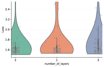
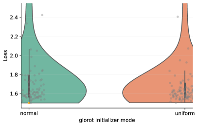
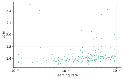
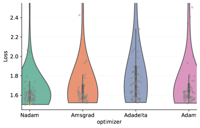
Figure 3.4: Graphical representation of the hyperoptimization loss function $L$ corresponding to a subset of the hyperparameters in a scan based on 1500 configurations.

In order to visualize a typical output of a hyperparameter scan, we show in Fig. 3.4 the result of a scan based on 1500 independent configurations. We display the hyperoptimization loss function $L$ (figure of merit), to be defined below, for a representative subset of hyperparameters: the depth of the network, the algorithm for the initialization of the network weights, the learning rate and the SGD optimizer variant. The smaller the value of the loss function $L$, the better this specific point is in the hyperparameter space. The full list of hyperparameters is given in Table 3.3. Note that here we only display the outcome of hyperparameter configurations that satisfy the post-fit selection cuts. The shape of the reconstructed probability distributions provides an indication of the stability of the results, with a wider distribution corresponding to a higher stability with respect to this specific hyperparameter.

In the specific case of the number of hidden layers of the network, one observes that the hyperoptimization algorithm identifies that it cannot further improve the figure of merit with one single layer, and accordingly it tests more configurations with two and three layers. The hyperparameter configurations corresponding to two and three layers appear to be equivalent in terms of the loss $L$, with a slightly better stability towards lower values in the two-layer case. No clear preference for a specific SGD variant is observed.

3.3.1 Figure of merit and stability

The complex interplay between hyperparameters indicates that a judicious choice of the figure of merit $L$ is crucial for the success of the hyperoptimization procedure. This figure of merit must relate to the quality of the fit: a possible choice would be setting the hyperoptimization loss to the validation $\chi^{2}$, that is, $L=\chi^{2}_{\text{val}}$. However, this quantity is already used in the stopping algorithm (Fig. 3.3) and hence using it may lead to hyperparameter configurations prone to over fitting [11] (“Goodhart’s law”, see Ref. [196]) . Rather, we define the loss $L$ through a $k$-fold cross validation method [197].

Figure 3.5: Diagrammatic representation of the $k$-fold algorithm used for the hyperparameter optimization.

A diagrammatic representation of the $k$-fold algorithm used for the hyperparameter optimization is displayed in Fig. 3.5. The hyperopt library generates a large number of hyperparameter configurations, and each of these is then used to produce fits to subsets of the experimental data. Specifically, for each point in the hyperparameter space we run $n_{\text{fold}}$ fits to the central experimental data, where $n_{\text{fold}}$ is the number of sets (folds) in which the data are being divided. We run a single fit to central data, rather than the standard set of around 100 replicas, because we prefer to scan over a very large number of hyperparameters, and fitting many replicas in each case would be computationally too intensive. In each of these $n_{\text{fold}}$ fits, the $k$-th fold is left out; the remaining folds are combined in a dataset which is then separated into training and validation in the usual way, such that the patience stopping of Fig. 3.3 can be tested.

The loss figure of merit $L$ is then defined as the average of the $\chi^{2}$ for the $k$-th, fold evaluated with the PDFs obtained in the $k$-th fit, in which this specific fold was left out, dubbed $\chi^{2}_{k}$ as illustrated in Fig. 3.5; that is

$$L={{1}\over{n_{\text{fold}}}}\displaystyle\sum^{n_{\text{fold}}}_{k=1}\chi_{k}^{2}\,.$$ (3.18)

We use the $n_{\rm fold}=4$ folds defined in Table 3.2. These are chosen in such a way that each fold is representative of the global dataset, both in terms of process type and kinematic coverage. The optimal hyperparameter set ${\boldsymbol{\hat{\theta}}}$ is then selected to be those that produce the lowest average loss computed using Eq. (3.18),

$$\boldsymbol{\hat{\theta}}=\underset{\boldsymbol{\theta}\in{\boldsymbol{\Theta}}}{\text{arg min}}\left({{1}\over{n_{\text{fold}}}}\displaystyle\sum^{n_{\text{fold}}}_{k=1}\chi_{k}^{2}({\boldsymbol{\theta}})\right).$$ (3.19)

We note that other choices of the loss function would be possible, such as

$$L={\rm max}\left(\chi_{1}^{2},\chi_{2}^{2},\chi_{3}^{2},\ldots,\chi_{n_{\rm fold}}^{2}\right),$$ (3.20)

namely, the maximum value of $\chi_{k}^{2}$ evaluated over the $n_{\rm fold}$ folds. We checked that results obtained with either choice are completely equivalent. In Fig. 3.6 we compare PDFs obtained by methodologies found by hyperoptimizing either with the “average” loss function of Eq. (3.18), or the “max” loss function of Eq. (3.20). The final hyperparameter values found in either case are provided in Table 3.3. It is clear that these final setups are quite different, yet the PDFs found with either methodology are indistinguishable. The fact that different choices for the hyperopt loss function $L$ result in rather different hyperparameter configurations that still produce indistinguishable PDFs demonstrates the stability of our methodology with respect to variations of the hyperoptimization procedure.

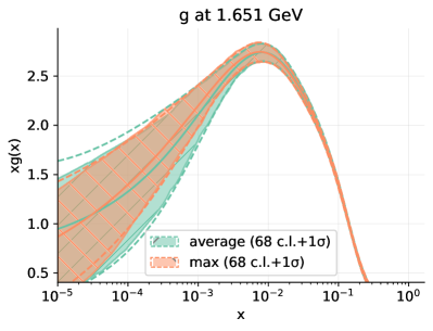
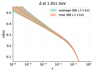
Figure 3.6: Comparison between the gluon (left) and antidown (right) PDFs at $Q=1.65$ GeV found by using methodologies in which hyperparameters are selected based on the “average” loss function Eq. (3.18) (green) or the “max” loss function Eq. (3.20) (orange).

Fold 1
CHORUS $\sigma_{CC}^{\nu}$	HERA I+II $\sigma_{\rm NC}^{p}\ e^{+}$ (920 GeV)	BCDMS $F_{2}^{p}$
LHCb $Z\to ee$ 7 TeV	ATLAS $W,Z$ 7 TeV ($\mathcal{L}=35$ pb-1)	CMS $Z$ $p_{T}$ 8 TeV
E605 $\sigma^{p}$	CMS DY 2D 7 TeV	CMS 3D dijets 8 TeV
ATLAS single $t$ 7 TeV ($1/\sigma d\sigma/dy_{\bar{t}}$)	ATLAS single $t$ $R_{t}$ 7 TeV	CMS $t\bar{t}~{}\ell$+jets 8 TeV ($1/\sigma d\sigma/dy_{t\bar{t}}$)
CMS single $t$ $R_{t}$ 8 TeV

Fold 2
HERA I+II $\sigma_{\rm CC}^{p}\ e^{-}$	HERA I+II $\sigma_{\rm NC}^{p}\ e^{+}$ (460 GeV)	HERA I+II $\sigma_{\rm NC}^{b}$
NMC $\sigma^{{\rm NC},p}$	NuTeV $\sigma_{CC}^{\bar{\nu}}$	LHCb $Z\to ee$ 8 TeV
CMS $W$ electron asymmetry 7 TeV	ATLAS $Z$ $p_{T}$ 8 TeV ($p_{T},m_{\ell\ell}$)	D0 W muon asymmetry
E866 $\sigma^{p}$ (NuSea)	ATLAS isolated $\gamma$ prod. 13 TeV	ATLAS dijets 7 TeV, R=0.6
ATLAS single $t$ 8 TeV ($1/\sigma d\sigma/dy_{\bar{t}}$)	CMS $\sigma_{tt}^{\rm tot}$ 7,8 TeV	CMS single $t$ $\sigma_{t}+\sigma_{\bar{t}}$ 7 TeV

Fold 3
HERA I+II $\sigma_{\rm CC}^{p}\ e^{+}$	HERA I+II $\sigma_{\rm NC}^{p}\ e^{+}$ (575 GeV)	NMC $F_{2}^{d}/F_{2}^{p}$
NuTeV $\sigma_{CC}^{\nu}$	LHCb $W,Z\to\mu$ 7 TeV	LHCb $Z\to ee$ 13 TeV
ATLAS $W,Z$ 7 TeV ($\mathcal{L}=4.6$ fb-1) central	ATLAS $W^{+}$+jet 8 TeV	ATLAS high-mass DY 7 TeV
CMS $W$ muon asymmetry 7 TeV	E866 $\sigma^{d}/2\sigma^{p}$ (NuSea)	CDF $Z$ differential
ATLAS $\sigma_{tt}^{\rm tot}$ 7,8 TeV	ATLAS single $t$ 8 TeV ($1/\sigma d\sigma/dy_{t}$)	CMS $\sigma_{tt}^{\rm tot}$ 5 TeV
CMS $t\bar{t}$ 2D $2\ell$ 8 TeV ($1/\sigma d\sigma/dy_{t}dm_{t\bar{t}}$)

Fold 4
CHORUS $\sigma_{CC}^{\bar{\nu}}$	HERA I+II $\sigma_{\rm NC}^{p}\ e^{+}$ (820 GeV)	LHCb $W,Z\to\mu$ 8 TeV
ATLAS $W,Z$ 7 TeV ($\mathcal{L}=4.6$ fb-1) forward	LHCb $Z\to\mu\mu$ 13 TeV	ATLAS $W^{-}$+jet 8 TeV
ATLAS low-mass DY 7 TeV	ATLAS $Z$ $p_{T}$ 8 TeV ($p_{T},y_{Z}$)	CMS $W$ rapidity 8 TeV
D0 $Z$ differential	CMS dijets 7 TeV	ATLAS single $t$ 8 TeV ($1/\sigma d\sigma/dy_{t}$)
ATLAS single $t$ $R_{t}$ 13 TeV	CMS single $t$ $R_{t}$ 13 TeV

Table 3.2: The four folds in which the NNPDF4.0 dataset is divided for the $k$-folds hyperoptimisation procedure represented in Fig. 3.4.

3.3.2 Hyperparameter correlation

An important motivation for the automated hyperparameter optimization procedure is the fact that the best value for a single hyperparameter cannot be determined independently of all the others, since there is a high degree of correlation between them. For instance, each variant of the SGD optimizer will have a different optimal value of the learning rate. We illustrate this interdependence with a specific hyperparameter, the clipnorm parameter of TensorFlow optimizers, for which a wrong choice can lead to significant overfitting even when all other hyperparameters are optimized. This parameter specifies the value at which to clip the norm of the gradient during a gradient descent step. That is, if the norm of the gradient at a given epoch is larger than the value of the clipnorm parameter, it will be rescaled such that the norm of the gradient used to update the neural network parameters has the clipnorm value.

The choice of clipnorm will affect the results of the optimization algorithm: if it is too small it can prevent convergence, while if it is too large the training will be unstable often leading to overfitting. In Fig. 3.7 we compare the strange PDF $xs(x,Q)$ at $Q=1.7$ GeV in the large-$x$ region for two variants of the NNPDF4.0 fit. In the first one, all the hyperparameters listed in Table 3.3 enter the hyperopt procedure, while in the second clipnorm is excluded and fixed by hand to an arbitrary value. While the two resulting hyperparameter configurations lead to similar values of the optimization figure of merit, the PDFs obtained in the latter case display undesirable overfitting behavior. This comparison illustrates the importance of including all relevant hyperparameters in the automated optimization.

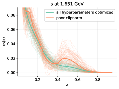
Figure 3.7: Comparison between the results for the strange PDF and large $x$ in two fits, one with all hyperparameters optimized and another where the clipnorm one is not hyperoptimized.

3.3.3 Baseline hyperparameters for NNPDF4.0

We have performed a $k$-folding hyperoptimization, as described above, and we have determined the best values of the hyperparameters that will be used for the NNPDF4.0 determination. These are listed in Table 3.3. The hyperparameters include the network architecture, the type of activation function, the Glorot-type [198] initializer, the optimizer, the values of the learning rate and of clipnorm, the maximum number of iterations and the stopping patience, and the initial values of the Lagrange multipliers for the PDF positivity and integrability constraints. The ranges of the hyperparameters that are sampled by the hyperoptimization algorithm are chosen empirically: we start out conservatively with very wide ranges, and once we are confident that the optimal value of a given hyperparameter falls within a sub-domain of this (conservative) range, we adjust the sampled domain accordingly to limit the runtime and computational resources of the hyperparameter scan.

Parameter	NNPDF4.0	$L$ as in Eq. (3.20)	Flavor basis Eq. (3.3)
Architecture	2-25-20-8	2-70-50-8	2-7-26-27-8
Activation function	hyperbolic tangent	hyperbolic tangent	sigmoid
Initializer	glorot_normal	glorot_uniform	glorot_normal
Optimizer	Nadam	Adadelta	Nadam
Clipnorm	6.0$\times 10^{-6}$	5.2$\times 10^{-2}$	2.3$\times 10^{-5}$
Learning rate	2.6$\times 10^{-3}$	2.5$\times 10^{-1}$	2.6$\times 10^{-3}$
Maximum # epochs	17$\times 10^{3}$	45$\times 10^{3}$	45$\times 10^{3}$
Stopping patience	10% of max epochs	12% of max epochs	16% of max epochs
Initial positivity $\Lambda^{(\rm pos)}$	185	106	2
Initial integrability $\Lambda^{\rm(int)}$	10	10	10

Table 3.3: The baseline hyperparameter configuration (left) selected using the $k$-folds hyperoptimization procedure with hyperoptimization loss Eq. (3.19) and used to perform the NNPDF4.0 fits in the evolution basis. We also show a configuration selected using the alternative hyperoptimization loss Eq. (3.20) (center) and the hyperparameter configuration employed to perform fits in the flavor basis, Eq. (3.3) (right).

In Table 3.3 we show both the optimal hyperparameters for our default methodology, based on the evolution basis and the hyperoptimization loss defined in Eq. (3.19), as well as the hyperparameter values obtained with the different choice of loss function Eq. (3.20), or with the same loss function but in the flavor basis. As mentioned both different choices of loss function (see Fig. 3.6) or a different choice of basis (see Sect. 8.4 below) lead to equivalent results, but the corresponding hyperparameter values can be quite different. For instance, the optimal architecture for fits based on the alternative loss function Eq. (3.20) has more than twice the number of neurons in the hidden layers compared to the baseline settings.

We now specifically discuss the hyperoptimization and its results for our default choice. Concerning the network architecture, until NNPDF3.1, each PDF was parametrized with an individual neural network. While the number of independently parametrized PDFs was gradually increased, this remained unchanged since NNPDF1.0 [199]. Now the hyperoptimization scan is run with a single network which outputs the value of all PDFs. So while in all NNPDF fits up to and including NNPDF3.1 ${\rm NN}_{k}(x;{\boldsymbol{\theta}})$ in Eq. (3.5) denotes the $k$-th neural network, in NNPDF4.0 it indicates the activation state of the $k$-th neuron in the last layer of the neural net. The architecture used in all previous NNPDF releases, namely 2-5-3-1 with sigmoid activation functions and a last linear layer is depicted in Fig. 3.8. The architecture selected by the hyperoptimization is 2-25-20-8 with hyperbolic activation functions except for the final linear layer, and it is shown in Fig. 3.9.

The NNPDF4.0 architecture has 763 free parameters, to be compared to a total of 296 parameters for the NNPDF3.1 neural nets. We emphasize however that a larger network does not necessarily imply better performance, and that for a given dataset there exists a lower bound to the number of required free network parameters but probably not an upper one. Given comparable performance, smaller networks are preferred in order to reduce the computational costs.

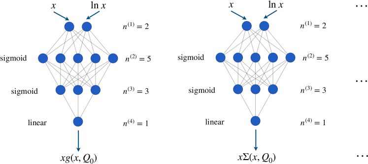
Figure 3.8: The neural network architecture adopted in all previous NNPDF determinations up to NNPDF3.1. Each independent PDF combination is parametrized by a separate neural network, all sharing a common architecture.

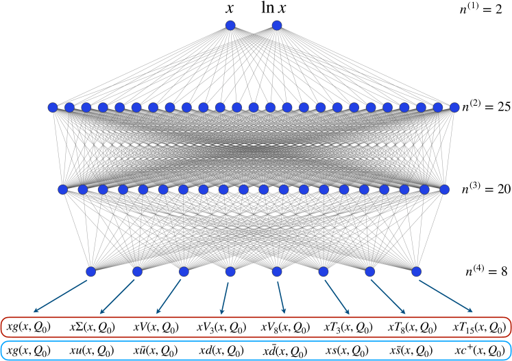
Figure 3.9: The neural network architecture adopted for NNPDF4.0. A single network is used, whose eight output values are the PDFs in the evolution (red) or the flavor basis (blue box). The architecture displayed corresponds to the optimal choice in the evolution basis; the optimal architecture in the flavor basis is different as indicated by Table 3.3).

The differences between the optimizer variants are quite subtle. While all optimizers exhibit a reasonable performance, it is also found that after hyperoptimization Nadam results in lower absolute losses $L$ than the other optimizers, while also appearing to be more stable. This further illustrates the benefits of hyperoptimization. Indeed, separately, the stability and general performance of all optimizers is quite similar, as can be seen in Fig. 3.4. This is something one might have also found by trial and error. However, a configuration Nadam that outperforms the other optimizers can be found thanks to the simultaneous sampling of different hyperparameters. This is something that cannot be concluded based on visual inspection of Fig. 3.4 and that would have been very difficult to establish by trial and error. It is supported by the fact that the top of the ranking of setups with the smallest losses is dominated by setups that use the Nadam optimizer.

3.3.4 Hyperoptimization stability

The main goal of the hyperoptimization procedure is to identify the best optimization settings for the current problem of determining the PDFs. This raises the question of deciding in which cases a new hyperoptimization would be required. Our current understanding encompasses changes to the experimental data, the theoretical description, and methodological choices (such as the choice of PDF basis).

We have checked that the procedure is quite stable upon reasonably small changes of the dataset. For instance, the appraisal and selection of the final dataset, see Sect. 4 below, did not require any new hyperoptimization. In fact, the datasets included in Table 3.2 do not correspond exactly to the datasets included in the final dataset, since the final appraisal of the data to be included was performed after the methodology was set. Furthermore, when removing datasets the given methodology remains viable, though in principle there might be a computationally more efficient one giving the same results for the small datasets. This will be seen explicitly in the context of “future tests” in Sect. 6.2 below. Of course in principle the only way of being absolutely certain whether a new hyperoptimization is needed or not is to actually perform it.

On the other hand, a substantial change in methodology or dataset generally needs a new hyperoptimization. This is illustrated by the fact (see Tab. 3.3) that the optimal settings for fitting in the flavor basis differ substantially from those of the evolution basis. Likewise, the addition of a large number of new datasets affecting kinematic regions or PDF combinations for which currently there is little or no information might have an impact on the fit sufficient to warrant a new run of the hyperoptimization procedure.

The open source NNPDF4.0 fitting framework released with this paper includes all necessary tools to carry out an automatic scan of hyperparameters, which means it can be readily used in situations which are very wildly different from the specific scenario considered in this work, be it in terms of the experimental data available or the theoretical framework being considered.

3.4 Performance and quality benchmarks

The new NNPDF fitting framework features a significantly improved computational performance compared to previous NNPDF. This improvement is mostly driven by the availability of the gradient-based optimizers provided by the TensorFlow library, combined with the dedicated hyperparameter optimization and other technical improvements in key parts of the code. Furthermore, the new fitting framework is able to take advantage of Graphical Processing Units (GPUs), which, when available, can further improve speed (although currently setting the same training and validation split for all replicas is needed for optimal performance).

	NNPDF3.1	NNPDF4.0 (CPU)	NNPDF4.0 (GPU)
Fit timing per replica	15.2 h	38 min	6.6 min
Speed up factor	1	24	140
RAM use	1.5 GB	6.1 GB	N/A

Table 3.4: The average fitting time per replica, speed up factor (as compared to the NNPDF3.1 performance), and the RAM requirements in global PDF fits based on the NNPDF3.1 and NNPDF4.0 frameworks for the same input dataset. In the NNPDF4.0 case, we compare the performance obtained on CPUs with that on GPUs.

To quantify the performance of the new fitting code, in Table 3.4 we show the average fitting time per replica in PDF fits based on the NNPDF3.1 and NNPDF4.0 fitting frameworks. The same global input dataset is used in both cases, in order to ensure a consistent comparison. In the case of NNPDF4.0, we compare the performances of running the code either in CPUs or in GPUs. These benchmark tests have been carried out on an Intel(R) Core(TM) i7-4770 at 3.40GHz CPU and on a NVIDIA Titan V GPU.

The comparisons in Table 3.4 show that, while in NNPDF3.1 the typical fitting time per Monte Carlo replica was around 15 hours, in NNPDF4.0 this has been reduced on average by a factor 24 (down to around 40 minutes) when running on CPUs, and by a factor of 140 (down to 7 minutes) when running on GPUs. This implies that, in the same time that it takes to run 100 replicas of NNPDF3.1, one can now run 2400 replicas of NNPDF4.0 or, alternatively, 24 variations (with different datasets or theory settings) of the same 100 NNPDF4.0 replicas. The enhanced performance of NNPDF4.0 is essential for the implementation of the hyperoptimization program: one can explore thousands of different hyperparameter configurations if the fits are fast enough. Furthermore, we note that this significant increase in speed greatly facilitates several physics applications, from the $\alpha_{s}(m_{Z})$ determination [138] to the simultaneous fits of PDFs and EFT Wilson coefficients [200, 201], which rely on producing a sufficiently large sample of replicas.

From Table 3.4 one can also observe that this increase in speed has as a trade-off a greater RAM memory consumption by around a factor of four. These demanding requirements arise because the code needs to hold in memory not only the FK-tables (as was already the case in NNPDF3.1) but also the $\chi^{2}$ gradients used for the minimization, which were not stored before. While this increase in memory may appear limiting, we note that the FK-tables and the functional form of the gradient can be shared between Monte Carlo replicas running simultaneously on the same processor. This makes it possible to run a large number of replicas in parallel on a GPU, and is the main reason for the reduction of the average fit time per replica reported in Table 3.4.

In addition to the improved computational performance, the new framework underlying the NNPDF4.0 fits exhibits other benefits that impact in a positive manner the actual outcome of the global fit. To illustrate these, Fig. 3.10 compares the distribution over replicas of the training lengths, defined as the optimal stopping point of each replica, between fits based on the NNPDF3.1 and NNPDF4.0 methodologies for a common dataset. While the number of iterations of the two different optimization algorithms are incomparable, it is interesting to note that the rightmost bin of the distribution is populated by the replicas whose stopping point is determined by the maximum number of iterations, rather than by satisfying the look-back cross-validation stopping condition. These are thus replicas for which full convergence has not been reached. The fact that replica training does stop through cross-validation is what guarantees that the $\chi^{2}$ minimzation is sufficiently accurate to actually determine the optimal fit.

From this comparison one finds that in NNPDF3.1, based on nodal genetic algorithms, around half of the replicas stop at the maximum number of generations, while for the SGD-based NNPDF4.0 fit this fraction is much smaller, around 15%. This observation implies that while in NNPDF3.1 many replicas might stop before proper training has been achieved, and may be affected by underlearning, this issue is much less severe in NNPDF4.0. Indeed, now 85% of the replicas stop when the optimal stopping point has been identified by the look-back cross-validation algorithm. One can therefore expect a reduction in the PDF uncertainties thanks to the new methodology, given that the fraction of replicas with potential underlearning is markedly reduced, leading to overall smoother and more similar replicas. We will study in more detail in Sect. 8 the impact at the PDF level of the new methodology.

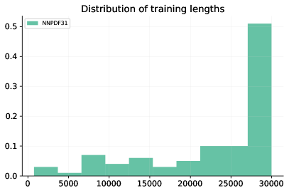
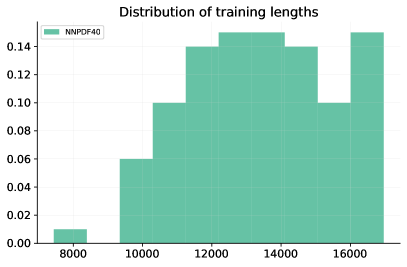
Figure 3.10: Distribution of training lengths, defined by the optimal stopping point of each replica, in fits to a common global dataset based on the NNPDF3.1 (left) and NNPDF4.0 (right panel) methodologies.

Similar considerations can be drawn from Fig. 3.11, which compares scatter plots with the values of $\chi^{2}_{\rm tr}$ and $\chi^{2}_{\rm val}$ for the $N_{\rm rep}=100$ replicas between fits based on the NNPDF3.1 and NNPDF4.0 methodologies and the same global dataset. In these plots, the red square indicates the position of the mean value over the replicas, and a dashed line with unit slope is added in order to facilitate visualization. Note that $\chi^{2}_{\rm val}$ is expected to be (on average) somewhat higher than $\chi^{2}_{\rm tr}$ given that validation data are not used for the optimization.

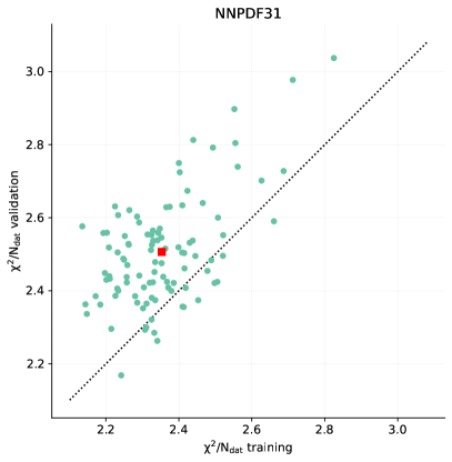
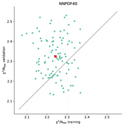
Figure 3.11: Comparison of the values of the training and validation $\chi^{2}$ for each replica between the NNPDF3.1 and NNPDF4.0 methodoligies, when fitting a common dataset. The red square indicates the mean value over the replicas.

From this comparison, one can see that the spread in the values of $\chi^{2}_{\rm tr}$ and $\chi^{2}_{\rm val}$ is reduced when going from NNPDF3.1 to NNPDF4.0. Furthermore, in the latter case there are no outliers, while this is not the case in the NNPDF3.1-like fits. Also, for NNPDF4.0 around one quarter of the replicas have $\chi^{2}_{\rm val}<\chi^{2}_{\rm tr}$, which is another indicator of proper training and stopping. This fraction is smaller in NNPDF3.1, again possibly signaling underlearning in some replicas.

All in all, the results presented in here indicate that the methodological improvements introduced in NNPDF4.0 not only lead to a significant improvement in terms of computational performance, but also to a more robust procedure where proper training is achieved for the majority of neural network replicas.

4 Determination of the baseline dataset

We discuss the selection criteria that we adopt to construct the NNPDF4.0 baseline dataset from the datasets described in Sect. 2. This baseline dataset will be used in all of the fits presented in the sequel. In previous PDF determinations, ad-hoc dataset selection criteria have often been applied. Here we strive to use objective criteria, not only for imposing kinematic cuts (which is standard), but also in order to select an optimal dataset for PDF determination out of the global dataset. We explain, in turn, our choice of kinematic cuts, our procedure to determine whether a measurement is to be included in the baseline dataset or not, and our selection of jet datasets, which deserve a separate treatment due to the need to choose the optimal observable.

4.1 Kinematic cuts

As in previous NNPDF analyses, kinematic cuts are imposed to ensure that we include only the data for which reliable predictions can be computed with fixed-order, pure QCD theory. In NNPDF3.1, see specifically Sect. 2 in [5], all the data points for which NNLO QCD corrections exceeded the corresponding experimental uncertainties were removed from the NLO fit. Likewise, all the data points for which electroweak (EW) corrections exceeded experimental uncertainties were removed from the NLO and NNLO fits. Additional cuts were also imposed on individual datasets on the basis of specific considerations. In the NNPDF4.0 analysis, kinematic cuts are determined on the ground of similar guiding principles, which we systematize as follows.

For the NLO fit, we discard datapoints that are subject to excessively large corrections: specifically, we compute, for each data point, the ratio between the absolute difference of the NNLO and NLO predictions to the experimental uncertainty. If this quantity is smaller than a given threshold value, the data point is retained in the NLO fit, otherwise it is discarded. We examined two alternative values of the threshold, $1$ and $2$ respectively. We concluded that a value of $1$ is unnecessarily aggressive, as it leads to discarding an excessive number of data points from the NLO fit, while a value of $2$ ensures that a reasonable number of data points are retained in the fit with reasonable theoretical accuracy. We therefore use $2$ as our default threshold value. On the other hand, we do not include in the NNLO fits the data points for which NNLO theory is not available. This is the case for the $W$+$c$ production measurements listed in Table 2.5. In this case, the full NNLO corrections to the dominant CKM-diagonal contribution have been recently computed in Ref. [87]. However the computation of Ref. [87] uses the flavor $k_{\perp}$ algorithm, which is not used in the experimental measurement, thus the NNLO corrections cannot be implemented yet in a PDF fit.

The results of Ref. [16] allow for a more refined analysis of cuts motivated by electroweak effects than what was possible in NNPDF3.1. We can now evaluate EW and mixed QCD+EW corrections in a systematic and consistent way for all hadronic processes included in a PDF fit, by taking advantage of the recent automation of these computations in mg5_aMC [124], and using of fast-interpolation grids with matching accuracy in the electroweak and strong couplings produced using PineAPPL [16]. We use the NNPDF3.1QED set [202] for the photon PDF [16]. We then exclude from the NLO and NNLO fits all data points for which the difference between the pure NLO QCD calculation and the full NLO QCD+EW computation (which includes the mixed corrections) exceeds the size of the experimental uncertainty. This strategy will also be used to investigate phenomenological implications of the NNPDF4.0 PDF sets in Sect. 9.

Dataset	NLO	NNLO
DIS measurements	$W^{2}\geq 12.5$ GeV2; $Q^{2}\geq 3.5$ GeV2	$W^{2}\geq 12.5$ GeV2; $Q^{2}\geq 3.5$ GeV2
HERA I+II $\sigma_{\rm NC}^{c}$ (in addition to the above)	—	$Q^{2}\geq 8$ GeV2 (fitted charm)
E866/E605 $\sigma^{p}$	$\tau\leq 0.08$; $|y/y_{\rm max}|\leq 0.0663$	$\tau\leq 0.08$; $|y/y_{\rm max}|\leq 0.0663$
D0 $W$ electron/muon asymmetry	—	$|A_{\ell}|\geq 0.03$
ATLAS low-mass DY 7 TeV	$m_{\ell\ell}>22$ GeV	—
ATLAS high-mass DY 7 TeV	$m_{\ell\ell}<210$ GeV	$m_{\ell\ell}<210$ GeV
CMS DY 2D 7 TeV	$30\leq m_{\ell\ell}\leq 200$ GeV; $|y_{\ell\ell}|\leq 2.2$	$m_{\ell\ell}\leq 200$ GeV; $|y_{\ell\ell}|\leq 2.2$
LHCb $W,Z\to\mu$ 7 TeV	—	$|\eta_{\mu}|/|y_{\mu\bar{\mu}}|\geq 2.25$
ATLAS low-mass DY 2D 8 TeV	$m_{\ell\ell}\leq 116$ GeV	$m_{\ell\ell}\leq 116$ GeV
LHCb $W,Z\to\mu$ 8 TeV	—	$|\eta_{\mu}|/|y_{\mu\bar{\mu}}|\geq 2.25$
LHCb $Z\to ee$/$Z\to\mu\mu$ 13 TeV	—	$|y_{\ell\ell}|\geq 2.25$
ATLAS $W^{\pm}$+jet 8 TeV	$p_{T}^{W}\geq 25$ GeV	$p_{T}^{W}\geq 25$ GeV
ATLAS $Z$ $p_{T}$ 8 TeV ($p_{T},m_{\ell\ell}$)	$p_{T}^{Z}\geq 30$ GeV	$p_{T}^{Z}\geq 30$ GeV
ATLAS $Z$ $p_{T}$ 8 TeV ($p_{T},y_{Z}$)	$30\leq p_{T}^{Z}\leq 150$ GeV	$30\leq p_{T}^{Z}\leq 150$ GeV
CMS $Z$ $p_{T}$ 8 TeV	$30\leq p_{T}^{Z}\leq 170$ GeV; $|y_{Z}|\leq 1.6$	$30\leq p_{T}^{Z}\leq 170$ GeV; $|y_{Z}|\leq 1.6$
CMS incl. jets 8 TeV	$p_{T}^{\rm jet}\geq 74$ GeV	$p_{T}^{\rm jet}\geq 74$ GeV

Table 4.1: The set of kinematic cuts applied to the datasets considered in the NNPDF4.0 PDF determination for the NLO and NNLO fits. The kinematic cuts used in the LO fit are the same as in the NLO fit. Only the data points that satisfy the constraints listed in the table are retained. The cut on the HERA I+II $\sigma_{\rm NC}^{c}$ dataset at NNLO is applied, in addition to the other cuts for DIS measurements, only when the charm PDF is independently parametrized.

Additional kinematic cuts are implemented for specific datasets, as summarized in Table 4.1. For datasets already included in NNPDF3.1, these are the same as in that analysis, see Sect. 2 in [5]. For new datasets, these follow from similar considerations. We summarize here the motivations. For DIS measurements the cuts remove the low-energy ($Q^{2}$) region, where perturbative QCD becomes unreliable, and the large invariant mass ($W^{2}$) region, where higher-twist corrections may be non-negligible. We impose a stricter $Q^{2}$ cut on the HERA I+II $\sigma_{\rm NC}^{c}$ dataset in the NNLO fit if the charm PDF is fitted in order to minimize the possible impact of missing NNLO terms related to initial-state charm (see Sect. 2.2 in [5]). For fixed-target DY measurements (specifically for E866 and E605 $\sigma^{p}$) the cuts remove the data points that are too close to the production threshold, as discussed in Ref. [5], based on the study of Ref. [203]. To this purpose, we define $\tau=m_{\ell\ell}^{2}/s$ and $y_{\rm max}=-{{1}\over{2}}\ln\tau$, where $m_{\ell\ell}$ is the invariant mass of the dilepton pair and $\sqrt{s}$ is the center-of-mass energy of the collision. For collider inclusive gauge boson production, we impose a cut on the D0 $W$ electron and muon asymmetry at NNLO because of the difficulty in obtaining a sufficiently precise theoretical prediction when the measured asymmetry becomes too close to zero; we exclude the lowest lepton rapidity bins of all of the LHCb measurements from the NNLO fit because, due to rapidity cut on the leptons ($y_{\ell}>2$) in the last bin the phase space for both leptons to pass the cut is very small, thus leading to numerical instabilities in the computation of the NNLO $K$-factor; and we remove the large invariant mass bins from the ATLAS low-mass DY 2D 8 TeV measurement in order to avoid overlap with the corresponding high-mass measurement. For $Z$ $p_{T}$ production we follow Ref. [204] and remove the largest rapidity bins from the CMS $Z$ $p_{T}$ 8 TeV measurement because of an apparent incompatibility with the corresponding ATLAS measurement, while fully retaining the latter.

All the remaining cuts displayed in Table 4.1 are imposed to remove data points for which $p_{T}$ resummation effects (typically in the low transverse momentum tail of the various distributions) or electroweak corrections (typically in the large transverse momentum or invariant mass tails of the various distributions) may become large. Finally, on top of the cuts listed in Table 4.1 we also apply at NLO a “similarity cut”: namely, if a datapoint is excluded at NNLO by one of the cuts in Table 4.1, then it is also excluded at NLO because the NLO to NNLO difference is unreliable so this point is potentially subject to large NNLO corrections.

Kinematic cuts in the LO fit are taken to be the same as in the NLO fit.

4.2 Baseline dataset

The datasets described in Sect. 2 and the kinematic cuts described in Sect. 4.1 above define an extended dataset out of which we determine a maximally consistent baseline dataset. This baseline dataset is determined through a new weighted-fit procedure that we introduce here. In this procedure, first we flag datasets that are problematic either in terms of fit quality, or because of the stability properties of their covariance matrix. This is done by comparing for each measurement respectively the value of the $\chi^{2}$ or the value of a stability indicator to a suitable threshold value. Measurements for which thresholds are exceeded are then subject to a dedicated weighted fit. The measurement is then retained or discarded based on the results of this weighted fit.

Below we will first discuss the issue of stability of covariance matrices and describe the stability indicator that we will use. We will then perform an appraisal of the full dataset of Sect. 2 based on our indicators and criteria. We will next present the weighted fit method, and finally apply it to our dataset and perform the final dataset selection based on it.

4.2.1 Stability of experimental covariance matrices

Given the high precision of modern collider experiments, in particular HERA and the LHC, many datasets are now limited by systematic, rather than statistical, uncertainties. In these situations, the $\chi^{2}$ of a given dataset often becomes extremely sensitive to small differences in the correlation model assumed for the experimental systematic errors. This implies that small inaccuracies in the estimate of the experimental correlated systematic uncertainties can potentially induce spurious disagreements between theory predictions and experimental data. Such spurious disagreements can complicate the interpretation of the quality of a PDF fit. A poor $\chi^{2}$ may be caused solely by an instability of the experimental covariance matrix upon its inversion, rather than by a genuine tension with the rest of the data in the fit, or by an inaccuracy in the theory.

In order to quantify the stability of the $\chi^{2}$ with respect to potential inaccuracies affecting the experimental covariance matrices, a new metric was derived in Ref. [205]. This metric has the key property of being independent of any theory predictions, and thus of the rest of the data in the fit, as it relies exclusively on the experimental covariance matrix as input. This property ensures it is independent of the actual fit quality (the value of the $\chi^{2}$). The metric is derived by studying the stability of the $\chi^{2}$ given ideally matching theory predictions, that is, when these are sampled from the same multi-Gaussian distribution as the experimental data.

Given the often limited information available on the details of some experimental systematic errors, this metric has to rely on some assumptions. The first one is that diagonal uncertainties are accurately known, and that potential instabilities are entirely explained by an imperfect knowledge of the correlations. The second is that the source of inaccuracies can be traced back to a $\mathcal{O}(1)$ number of specific entries in the correlation matrix. An example of the latter assumption would be an inaccuracy in the estimate of the correlation between two data bins in opposite kinematic regions.

Under these assumptions, one can decompose [205] the experimental covariance matrix $C$ as

$$C=DRD\,,$$ (4.1)

where $D$ is a diagonal matrix whose entries are the square roots of the diagonal entries in the covariance matrix, i.e. the standard deviations, and $R$ is the correlation matrix. If the smallest eigenvalue of the correlation matrix $R$ is $\lambda_{0}$, then the stability of the $\chi^{2}$ with respect to the inaccuracies of the experimental correlation model will be quantified by the condition number

$$Z=\lambda_{0}^{-{{1}\over{2}}}\,.$$ (4.2)

The value of $(\sqrt{2}Z)^{-1}$ can be related to an estimate of the required precision at which correlations need to be determined in order to ensure that they affect the $\chi^{2}$ statistic by less than one standard deviation, that is, by less than $\sigma_{\chi^{2}}=\sqrt{2/N_{\rm dat}}$ when normalized by the number of data points

For example, a value of $Z=5$ of the metric indicates that correlations must be estimated with an absolute uncertainty of less than $0.14$. This means that if the correlation between two bins is estimated to be 1.0 while its real value is instead 0.86, one can expect that the $\chi^{2}$ may deviate significantly from unity (by more than $\sigma_{\chi^{2}}$) even if the experimental data and theory calculations are perfectly consistent.

Therefore, by evaluating the datasets in the global fit with a relatively large value of the stability metric $Z$, one can identify those with a potentially unstable correlation matrix. If in addition these datasets display a poor fit quality, further investigation is required since a high value of the $\chi^{2}$ does not necessarily indicate a genuine tension in the data or a limitation of the theory calculations, but rather it could arise from the instability of the experimental covariance matrix.

In the remainder of this section, we will use the stability metric $Z$ as a diagnostic tool to flag datasets that deserve further investigation. A regularization procedure in order to correct a covariance matrix with large $Z$ can also be constructed [205]. Such a regularization procedure is not implemented in the default NNPDF4.0 fit, rather it will be implemented in Sect. 8.7 in order to assess the possible impact on the PDFs of regularizing the covariance matrix for those datasets characterized by large $Z$ values.

4.2.2 Appraisal and selection criteria

We perform an appraisal of the full dataset discussed in Sect. 2 with the goal of determining its internal consistency. Specific measurements could be inconsistent with the rest of the dataset due to a variety of reasons of theoretical or experimental origin, such as for example large missing higher order QCD or electroweak corrections, missing systematic uncertainties, or underestimated experimental uncertainties. Our goal is not to attempt to have a full understanding of the nature of the inconsistencies, but rather, to single out and exclude from the baseline inconsistent data based on objective criteria. These data can then be studied separately through dedicated fits.

We start by performing a NNLO fit in which the full dataset is used. This fit adopts the theory settings discussed in Sect. 2, it implements the kinematic cuts of Sect. 4.1, and it is based on the methodology described in Sect. 3. For jet observables, it is impossible to include simultaneously dijets and single-inclusive jets because experimental correlations between them are not available. In this baseline fit, as well as in our default analysis, we choose to include dijets (and not single-inclusive jets) at 7 TeV and single-inclusive jet (and not dijets) at 8 TeV. The motivation for this choice will be presented in a separate analysis in Sect. 4.3.

We then consider, for each measurement, the following indicators and apply the following selection criteria:

• The total $\chi^{2}$ per data point. We single out all the datasets for which $\chi^{2}>1.5$. An excess from the expected unit value of the $\chi^{2}$ could arise from dataset inconsistencies, within the dataset or between the dataset and the rest of the extended dataset, from inaccuracies of the theoretical computations, from large statistical fluctuations (especially for datasets with a small number of data points) or from instabilities of the experimental covariance matrix.

• The number of standard deviations $n_{\sigma}$ by which the value of the $\chi^{2}$ per data point differs from the expected unit value,

  $$n_{\sigma}\equiv{{\chi^{2}-1}\over{\sigma_{\chi^{2}}}}={{\chi^{2}-1}\over{\sqrt{2/N_{\rm dat}}}}.$$ (4.3)

  We single out all the datasets for which $|n_{\sigma}|>2$. In these cases, the statistical significance of an anomalously large $\chi^{2}$ might not be explained by a statistical fluctuation.

• The stability metric $Z$ defined in Eq. (4.2). We single out the datasets with $Z>4$. This choice is based on the regularization studies performed in [205], which find that by minimally altering the correlation model such that they fulfill $Z=4$, the induced changes in the resulting covariance matrix are very likely within the precision to which they were determined. The observed differences between the regularized and unregularized covariance matrices are $5\%$ for the standard deviations and below 0.05 (in absolute units) for the correlation coefficients.

The first estimator flags all situations in which the significance of the discrepancy does not depend on the number of data points, such as for instance a missing higher order correction that affects all data points. The latter two instead are sensitive to cases in which there might be issues related to systematic uncertainties and their correlation, whose significance depends on the number of data points.

Dataset	$N_{\rm dat}$	$\chi^{2}$	$n_{\sigma}$	$Z$	$\omega$	decision
NMC $F_{2}^{d}/F_{2}^{p}$	121	0.87	$-1.02$	1.098	—
NMC $\sigma^{{\rm NC},p}$	204	1.53	$+5.33$	2.743	23	retain
SLAC $F_{2}^{p}$	33	0.96	$-0.16$	1.731	—
SLAC $F_{2}^{d}$	34	0.62	$-1.55$	1.566	—
BCDMS $F_{2}^{p}$	333	1.42	$+5.42$	4.456	14	retain
BCDMS $F_{2}^{d}$	248	1.01	$+0.13$	3.468	—
CHORUS $\sigma_{CC}^{\nu}$	416	0.95	$-0.66$	4.132	—
CHORUS $\sigma_{CC}^{\bar{\nu}}$	416	0.87	$-1.85$	2.073	—
NuTeV $\sigma_{CC}^{\nu}$ (dimuon)	39	0.35	$-2.88$	1.092	—
NuTeV $\sigma_{CC}^{\bar{\nu}}$ (dimuon)	37	0.58	$-1.80$	1.043	—
HERA I+II $\sigma_{\rm NC}^{p}\ e^{-}$	159	1.40	$+3.54$	1.647	—
HERA I+II $\sigma_{\rm NC}^{p}\ e^{+}$ (460 GeV)	204	1.08	$+0.78$	1.739	—
HERA I+II $\sigma_{\rm NC}^{p}\ e^{+}$ (575 GeV)	254	0.90	$-1.11$	1.639	—
HERA I+II $\sigma_{\rm NC}^{p}\ e^{+}$ (820 GeV)	70	1.11	$+0.62$	2.004	—
HERA I+II $\sigma_{\rm NC}^{p}\ e^{+}$ (920 GeV)	377	1.30	$+4.06$	1.845	—
HERA I+II $\sigma_{\rm CC}^{p}\ e^{+}$	42	1.27	$+1.23$	1.165	—
HERA I+II $\sigma_{\rm CC}^{p}\ e^{-}$	39	1.23	$+1.01$	1.101	—
HERA I+II $\sigma_{\rm NC}^{c}$	37	2.03	$+4.45$	1.629	127	retain
HERA I+II $\sigma_{\rm NC}^{b}$	26	1.43	$+1.56$	1.299	—

Table 4.2: The DIS datasets in the NNPDF4.0 fit to the extended dataset. For each dataset we show the number of data points, the $\chi^{2}$ per data point, the corresponding number of standard deviations $n_{\sigma}$ and the stability metric $Z$, and the value of the weight $\omega$ used in the definition of the weighted fit $\chi^{2}$ in Eq. (4.4). In the last column, we also indicate whether this dataset is retained in the NNPDF4.0 baseline dataset.

Dataset	$N_{\rm dat}$	$\chi^{2}$	$n_{\sigma}$	$Z$	$\omega$	decision
E866 $\sigma^{p}$ (NuSea)	89	1.60	$+3.95$	1.789	53	retain
E866 $\sigma^{d}/2\sigma^{p}$ (NuSea)	18	0.53	$-1.30$	1.428	—
E605 $\sigma^{p}$	85	0.45	$-3.56$	1.627	—
E906 $\sigma^{d}/2\sigma^{p}$ (SeaQuest)	6	0.87	$-0.22$	1.963	—

Table 4.3: Same as Table 4.2 for fixed-target DY data.

Dataset	$N_{\rm dat}$	$\chi^{2}$	$n_{\sigma}$	$Z$	$\omega$	decision
CDF $Z$ differential	29	1.23	$+0.87$	5.966	—
D0 $Z$ differential	28	0.65	$-1.31$	1.000	—
D0 $W$ electron asymmetry	11	3.54	$+5.97$	1.939	429	remove
D0 $W$ muon asymmetry	9	1.64	$+1.35$	1.402	—
ATLAS low-mass DY 7 TeV	6	0.89	$-0.18$	3.696	—
ATLAS high-mass DY 7 TeV	5	1.67	$+1.06$	3.110	—
ATLAS $W,Z$ 7 TeV ($\mathcal{L}=35$ pb-1)	30	0.94	$-0.24$	3.451	—
ATLAS $W,Z$ 7 TeV ($\mathcal{L}=4.6$ fb-1) central	46	1.86	$+4.13$	9.013	102	retain
ATLAS $W,Z$ 7 TeV ($\mathcal{L}=4.6$ fb-1) forward	15	1.04	$+0.10$	2.838	—
CMS $W$ electron asymmetry 7 TeV	11	0.97	$-0.07$	1.061	—
CMS $W$ muon asymmetry 7 TeV	11	1.69	$+1.61$	1.246	—
CMS DY 2D 7 TeV	110	1.34	$+2.50$	8.785	—
LHCb $Z\to ee$ 7 TeV	17	1.25	$+0.72$	1.436	—
LHCb $W,Z\to\mu$ 7 TeV	29	2.32	$+5.04$	2.890	162	retain
ATLAS $W$ 8 TeV	22	3.50	$+8.29$	11.28	214	remove
ATLAS low-mass DY 2D 8 TeV	60	1.26	$+1.42$	1.120	—
ATLAS high-mass DY 2D 8 TeV	48	1.11	$+0.53$	2.568	—
CMS $W$ rapidity 8 TeV	22	1.20	$+0.65$	13.51	—
LHCb $Z\to ee$ 8 TeV	17	1.25	$+0.72$	1.436	—
LHCb $W,Z\to\mu$ 8 TeV	30	1.39	$+1.51$	2.542	—
LHCb $W\to e$ 8 TeV	8	2.61	$+3.22$	1.005	590	remove
ATLAS $\sigma_{W,Z}^{\rm tot}$ 13 TeV	3	0.97	$-0.03$	4.961	—
LHCb $Z\to ee$ 13 TeV	16	0.94	$-0.16$	2.354	—
LHCb $Z\to\mu\mu$ 13 TeV	15	1.66	$+1.80$	1.608	—

Table 4.4: Same as Table 4.2 for collider (Tevatron, top, and LHC, bottom) inclusive gauge boson production data.

Dataset	$N_{\rm dat}$	$\chi^{2}$	$n_{\sigma}$	$Z$	$\omega$	decision
ATLAS $W^{+}$+jet 8 TeV	15	0.76	$-0.65$	4.020	—
ATLAS $W^{-}$+jet 8 TeV	15	1.50	$+1.36$	5.679	—
ATLAS $Z$ $p_{T}$ 8 TeV ($p_{T},m_{\ell\ell}$)	44	0.91	$-0.42$	3.325	—
ATLAS $Z$ $p_{T}$ 8 TeV ($p_{T},y_{Z}$)	48	0.89	$-0.52$	8.815	—
CMS $Z$ $p_{T}$ 8 TeV	28	1.38	$+1.41$	9.521	—
CMS $\sigma_{tt}^{\rm tot}$ 5 TeV	1	0.42	$-0.41$	1.000	—
ATLAS $\sigma_{tt}^{\rm tot}$ 7 TeV	1	3.66	$+1.88$	1.000	—
CMS $\sigma_{tt}^{\rm tot}$ 7 TeV	1	0.58	$-0.30$	1.000	—
ATLAS $\sigma_{tt}^{\rm tot}$ 8 TeV	1	0.03	$-0.71$	1.000	—
CMS $\sigma_{tt}^{\rm tot}$ 8 TeV	1	0.07	$-0.66$	1.000	—
ATLAS $\sigma_{tt}^{\rm tot}$ 13 TeV ($\mathcal{L}$=139 fb-1)	1	0.33	$-0.47$	1.000	—
CMS $\sigma_{tt}^{\rm tot}$ 13 TeV	1	0.13	$-0.61$	1.000	—
ATLAS $t\bar{t}~{}\ell$+jets 8 TeV ($1/\sigma d\sigma/dp_{T}^{t}$)	7	4.11	$+5.82$	5.165	674	remove
ATLAS $t\bar{t}~{}\ell$+jets 8 TeV ($1/\sigma d\sigma/dy_{t}$)	4	3.61	$+3.69$	1.653	1180	retain
ATLAS $t\bar{t}~{}\ell$+jets 8 TeV ($1/\sigma d\sigma/dy_{t\bar{t}}$)	4	3.81	$+3.97$	2.185	1180	retain
ATLAS $t\bar{t}~{}\ell$+jets 8 TeV ($1/\sigma d\sigma/dm_{t\bar{t}}$)	6	1.86	$+1.50$	8.070	786	remove
ATLAS $t\bar{t}~{}2\ell$ 8 TeV ($1/\sigma d\sigma/dy_{t\bar{t}}$)	5	1.53	$+0.84$	1.907	—
CMS $t\bar{t}~{}\ell$+jets 8 TeV ($1/\sigma d\sigma/dy_{t\bar{t}}$)	9	1.35	$+0.74$	1.628	—
CMS $t\bar{t}$ 2D $2\ell$ 8 TeV ($1/\sigma d\sigma/dy_{t}dm_{t\bar{t}}$)	16	0.93	$-0.19$	2.908	—
CMS $t\bar{t}~{}\ell$+jet 13 TeV ($d\sigma/dy_{t}$)	10	0.53	$-1.05$	5.163	—
CMS $t\bar{t}~{}2\ell$ 13 TeV ($d\sigma/dy_{t}$)	11	0.69	$-0.72$	7.486	—
ATLAS incl. jets 8 TeV, R=0.6	171	0.71	$-2.68$	5.476	—
CMS incl. jets 8 TeV	185	1.20	$+1.96$	6.273	—
ATLAS dijets 7 TeV, R=0.6	90	2.16	$+7.76$	9.936	52	retain
CMS dijets 7 TeV	54	1.85	$+4.42$	4.695	87	retain
ATLAS isolated $\gamma$ prod. 8 TeV	49	2.03	$+5.09$	7.277	—	remove
ATLAS isolated $\gamma$ prod. 13 TeV	53	0.75	$-1.31$	1.304	—
ATLAS single $t$ $R_{t}$ 7 TeV	1	0.40	$-0.42$	1.000	—
CMS single $t$ $\sigma_{t}+\sigma_{\bar{t}}$ 7 TeV	1	0.71	$-0.20$	1.000	—
CMS single $t$ $R_{t}$ 8 TeV	1	0.13	$-0.61$	1.000	—
ATLAS single $t$ $R_{t}$ 13 TeV	1	0.04	$-0.68$	1.000	—
CMS single $t$ $R_{t}$ 13 TeV	1	0.31	$-0.49$	1.000	—
ATLAS single $t$ 7 TeV ($1/\sigma d\sigma/dy_{t}$)	3	0.95	$-0.06$	1.281	—
ATLAS single $t$ 7 TeV ($1/\sigma d\sigma/dy_{\bar{t}}$)	3	0.06	$-1.15$	1.385	—
ATLAS single $t$ 8 TeV ($1/\sigma d\sigma/dy_{t}$)	3	0.25	$-0.92$	1.197	—
ATLAS single $t$ 8 TeV ($1/\sigma d\sigma/dy_{\bar{t}}$)	3	0.19	$-0.99$	1.230	—

Table 4.5: Same as Table 4.2 for other LHC processes (listed in Table 2.5).

The number of data points $N_{\rm dat}$ and the values of the three estimators outlined above are collected, for each measurement, in Tables 4.2-4.5. We flag the datasets that have both $\chi^{2}>1.5$ and $|n_{\sigma}|>2$ or $|n_{\sigma}|>2$ and $Z>4$. These datasets will be investigated through the weighted fit method presented in Sect. 4.2.3 below. The only exception is the ATLAS isolated photon production measurement at 8 TeV which is discarded given that it is superseded by the companion measurement at 13 TeV. We do not flag datasets with $\chi^{2}>1.5$ but with $|n_{\sigma}|<2$, nor the datasets with with $Z>4$ but with $|n_{\sigma}|<2$. In the first case the large value of the $\chi^{2}$ is consistent with a statistical fluctuation. In the second case despite its unstable covariance matrix the dataset can nevertheless be fitted with acceptable fit quality. Datasets characterized by large $Z$ values will be further investigated in Sect. 8.7 below, where their impact on the PDFs will be reassessed by means of a suitable regularization procedure that reduces their $Z$ value.

The datasets that are flagged according to these criteria are singled out in Tables 4.2-4.5 by the presence of a weight in the penultimate column. These are: NMC and BCDMS proton structure functions; combined HERA charm structure function; D0 $W$ electron asymmetry; 7 TeV ATLAS $W,Z$ central rapidity; 8 TeV ATLAS $W$ rapidity; 7 TeV LHCb $W$; 8 TeV LHCb electron asymmetry; 8 TeV ATLAS lepton+jets top-pair; and 7 TeV ATLAS and CMS dijet.

These datasets are hence potentially inconsistent, and they are assessed using the weighted fit method as discussed below. All other datasets listed in Tables 4.2-4.5 are deemed to be consistent and thus included in the NNPDF4.0 baseline.

4.2.3 The weighted fit method

The weighted fit method is based on the idea that in order to determine whether a specific measurement is inconsistent with the global dataset one should produce a PDF determination that provides the best agreement to this dataset. One may then check whether this best agreement does or does not lead to the deterioration of the agreement with one or more of the other data included in the global dataset. This idea was recently used in Ref. [206] as a means of studying the determination of standard model parameters, such as the strong coupling $\alpha_{s}(m_{Z})$, from a global PDF fit. Related methods were previously discussed in Ref. [207].

The way the idea is implemented is by performing a weighted fit, in which the selected dataset is given a weight that is large enough for it to carry about the same weight as the rest of the global dataset. To this goal, the figure of merit optimized in the fit is modified as

$$\chi^{2}={{1}\over{N_{\rm dat}}}\sum_{i=1}^{n_{\rm exp}}N_{\rm dat}^{(i)}\chi^{2}_{i}\qquad\longrightarrow\qquad\chi^{2}={{1}\over{N_{\rm dat}-N_{\rm dat}^{(j)}}}\sum_{i\neq j}^{n_{\rm exp}}N_{\rm dat}^{(i)}\chi^{2}_{i}+\omega^{(j)}\chi^{2}_{j}\,,$$ (4.4)

where $N_{\rm dat}^{(i)}$ is the number of data points in the dataset $i$ and $\chi^{2}_{i}$ is the contribution to the total $\chi^{2}$ from the given dataset. The value of $\omega^{(j)}$ is then chosen as

$$\omega^{(j)}=N_{\rm dat}/N_{\rm dat}^{(j)}.$$ (4.5)

The last column of Tables 4.2-4.5 lists the values of $\omega^{(j)}$ for the datasets that we have singled out according to the criteria discussed above. We have explicitly checked that the choice of the precise value of $\omega^{(j)}$ does not change the general conclusions, by repeating several weighted fits with two more choices of $\omega^{(j)}$, namely, twice or half the default value defined by Eq. (4.5).

The possible outcomes of a weighted fit, and the corresponding conclusions on dataset compatibility, are the following:

• The value of $\chi^{2}_{j}$ does not improve significantly while the $\chi^{2}_{i}$ of the rest of the datasets remain essentially unaffected. In this case we conclude that the dataset $j$ exhibits internal inconsistencies that however do not distort the global fit. We keep dataset $j$ in the baseline.

• The value of $\chi^{2}_{j}$ does not improve significantly and the $\chi^{2}_{i}$ of several of other datasets, including those belonging to the same process type of dataset $j$, worsen significantly. In this case we conclude that the internal inconsistencies of the given dataset distort the global fit. We remove dataset $j$ from the baseline.

• The value of $\chi^{2}_{j}$ improves significantly and the $\chi^{2}_{i}$ of the rest of the dataset is unchanged within statistical fluctuations. In this case we conclude that the dataset $j$ was not fitted properly because it carries a small weight in the fit. We keep dataset $j$ in the baseline.

• The value of $\chi^{2}_{j}$ improves significantly but the $\chi^{2}_{i}$ of several of other datasets, including those belonging to the same process type of dataset $j$, worsen significantly. In this case we conclude that the given dataset is inconsistent with the global dataset. We remove dataset $j$ from the baseline.

The appraisal, to be presented in Sect. 4.2.4 below, must be done on a case-by-case basis, as there are several factors, rather than a single figure of merit, that determine whether or not the fit quality to other datasets worsens significantly, such as, for instance, whether the $\chi^{2}$ that worsens corresponds to data from the same process type or sensitive to the same PDF, whether there are known issues related to missing higher order or resummation corrections, etc. In all cases which are not clear-cut, we keep the dataset under consideration.

4.2.4 Appraisal and selection

Table 4.6 reports the values of the $\chi^{2}$ obtained in the weighted fits for both the weighted dataset and for the rest of the datasets in the fit, grouped by process. In the latter, the $\chi^{2}$ includes the contribution coming from the weighted dataset (if the weighted dataset belongs to the process), but with $\omega^{(i)}=1$ in Eq. (4.4). For ease of reference, we also reproduce (in parenthesis) the values of the $\chi^{2}$ in the unweighted fit originally used to assess each dataset, as given in Tables 4.2-4.5.

	Weighted dataset	DIS (fixed-target)	DIS (collider)	DY (fixed-target)	$W,Z$ prod. (inclusive)	$W,Z$ prod. ($p_{T}$ and jets)	Top pair prod.	Jet prod.	Isolated $\gamma$ prod.	Single $t$ prod.	Total
Unweighted fit	—	1.06	1.20	0.99	1.48	0.98	1.51	1.28	1.36	0.35	1.20
NMC $\sigma^{NC,p}$	1.28 (1.53)	1.07	1.22	0.94	1.51	1.00	1.74	1.25	1.33	0.36	1.21
BCDMS $F_{2}^{p}$	1.05 (1.42)	1.11	1.29	1.01	1.68	0.98	1.50	1.32	1.49	0.37	1.28
HERA I+II $\sigma_{\rm NC}^{c}$	1.37 (2.03)	1.07	1.45	0.99	1.62	1.01	1.68	1.25	1.29	0.38	1.30
E866 $\sigma^{p}$ (NuSea)	0.90 (1.60)	1.11	1.23	0.72	1.65	0.96	1.51	1.30	1.31	0.39	1.24
D0 $W$ electron asymmetry	1.94 (3.54)	1.12	1.23	1.18	1.70	0.97	1.52	1.37	1.37	0.38	1.28
ATLAS $W,Z$ 7 TeV ($\mathcal{L}=4.6$ fb-1) central	1.23 (1.86)	1.13	1.31	0.96	1.60	1.00	1.56	1.33	1.33	0.37	1.27
LHCb $W,Z\to\mu$ 7 TeV	0.77 (2.32)	1.13	1.23	1.02	1.65	1.04	1.39	1.40	1.28	0.42	1.27
ATLAS $W$ 8 TeV	1.11 (3.50)	1.16	1.28	1.07	1.59	1.03	1.43	1.37	1.33	0.36	1.30
LHCb $W\to e$ 8 TeV	0.19 (2.61)	1.11	1.22	1.17	1.79	1.00	1.42	1.33	1.36	0.34	1.29
ATLAS $t\bar{t}~{}\ell$+jets 8 TeV ($1/\sigma d\sigma/dp_{T}^{t}$)	1.21 (4.11)	1.52	1.40	1.05	2.12	1.38	1.82	2.60	2.14	0.69	1.73
ATLAS $t\bar{t}~{}\ell$+jets 8 TeV ($1/\sigma d\sigma/dy_{t}$)	0.68 (3.61)	1.09	1.22	1.07	1.52	0.97	2.10	1.51	1.32	0.37	1.26
ATLAS $t\bar{t}~{}\ell$+jets 8 TeV ($1/\sigma d\sigma/dy_{t\bar{t}}$)	1.67 (3.81)	1.11	1.24	0.89	1.58	0.95	1.63	1.63	1.31	0.39	1.28
ATLAS $t\bar{t}~{}\ell$+jets 8 TeV ($1/\sigma d\sigma/dm_{t\bar{t}}$)	1.32 (1.86)	1.23	1.30	1.15	1.74	1.00	4.06	1.73	1.76	0.55	1.47
ATLAS dijets 7 TeV, R=0.6	1.84 (2.16)	1.08	1.21	0.99	1.61	0.98	2.50	1.39	1.38	0.40	1.25
CMS dijets 7 TeV	1.34 (1.85)	1.08	1.20	0.93	1.63	0.99	1.77	1.28	1.33	0.35	1.22

Table 4.6: The $\chi^{2}$ obtained in the unweighted (first row) and weighted fits (rest of the table) to the extended dataset. In each of the weighted fits the dataset indicated in the first column receives the weight reported in Tables 4.2-4.5. For each fit, the second column reports the $\chi^{2}$ of the weighted dataset in the weighted fit. The value in the unweighted fit (same as in Tables 4.2-4.5) is also given for reference in parenthesis. The other columns display the $\chi^{2}$ of subsets of datasets, grouped by process, in the weighted fits. These values include the contribution from the weighted dataset but with $\omega^{(i)}=1$ in Eq. (4.4).

Based on Table 4.6, we reach to the following conclusions, which are also summarized in the last column of Tables 4.2-4.5.

• NMC $\sigma^{NC,p}$. The $\chi^{2}$ of this dataset improves from 1.53 to 1.28. The $\chi^{2}$ of the other datasets and the total $\chi^{2}$ fluctuate only marginally. These results are consistent with those reported in [208, 209, 210] and confirm that this dataset is internally inconsistent. Because such an inconsistency does not alter the global fit significantly, we keep this dataset in the baseline.

• BCDMS $F_{2}^{p}$. The $\chi^{2}$ of this dataset improves from 1.42 to 1.05. The total $\chi^{2}$ worsens, however this worsening is moderate and it does not seem to come from any specific process. These results confirm a mild inconsistency of this dataset with the rest of the datasets in the fit, which however does not appear to be significant enough to justify its removal from the fit. We thus keep this dataset in the baseline.

• HERA I+II $\sigma_{\rm NC}^{c}$. The $\chi^{2}$ of this dataset improves from 2.03 to 1.37, but the agreement with all the other HERA data, driven by the inclusive structure function measurements, deteriorates, with a $\chi^{2}$ increase from 1.20 to 1.45. The $\chi^{2}$ of all of the other datasets fluctuate only marginally. We therefore conclude that this dataset is in tension with the small-$x$ HERA inclusive structure function, as also observed in the CT18 and MSHT20 analyses [143, 144]. This tension will possibly be alleviated once small-$x$ resummation effects are accounted for [211], though only a resummed PDF determination could tell whether this is the case or not. Nevertheless the PDFs in the global fit remain unchanged if the dataset is removed. Furthermore, this dataset is required in order to stabilize the charm PDF, especially in a DIS-only fit, as we will discuss in Sect. 7. For these reasons we keep the measurement in the baseline.

• E866 $\sigma^{p}$ (NuSea). The $\chi^{2}$ of this dataset improves from 1.59 to 0.90. The $\chi^{2}$ of inclusive gauge boson production deteriorates somewhat, from 1.48 to 1.65. A possible reason for this is the lack of large-$x$ resummation in the treatment of the theoretical predictions for this dataset [203]. Mild inconsistency of this experiment with NMC was argued in Ref. [212]. Nevertheless, the fit quality of this dataset in the original unweighted fit is only marginally above our selection criteria, and the deterioration of the global $\chi^{2}$ is also marginal. We keep it in the baseline.

• D0 $W$ electron asymmetry. The $\chi^{2}$ of this dataset improves from 3.54 to 1.94, a value that remains sub-optimal. The $\chi^{2}$ of all of the other datasets, in particular of those belonging to the same process (including the D0 $W$ muon asymmetry), deteriorates very significantly. The dataset is surely inconsistent, though perhaps the inconsistency can be traced to a single data point. We discard the dataset from the baseline.

• ATLAS $W,Z$ 7 TeV ($\mathcal{L}=4.6$ fb^-1) (central rapidity range). The $\chi^{2}$ of this dataset improves from 1.86 to 1.23 while the overall $\chi^{2}$ of collider gauge boson production data deteriorates slightly, from 1.48 to 1.60. However, this deterioration is very moderate, and furthermore, as we will show in Sect. 8, a small amount of regularization of experimental correlations significantly improve the description of the dataset while leaving the PDFs unchanged. There is thus no evidence that this dataset is inconsistent, and we keep it in the baseline.

• LHCb $Z\to ee$ 7 TeV. The $\chi^{2}$ of this dataset improves from 2.32 to 0.77. At the same time the $\chi^{2}$ of all collider gauge boson production data deteriorates slightly from 1.48 to 1.65. Given the moderate amount of deterioration it is unclear that this dataset is inconsistent and we keep it in the baseline.

• ATLAS $W$ 8 TeV. The $\chi^{2}$ of this dataset improves from 3.50 to 1.11 but the description of the other datasets, except top pair production, deteriorates quite significantly. As in the case of the companion measurement at 7 TeV, given the large value of $Z$, we will investigate in Sect. 8 whether the description of this experiment could be improved by regularization of its covariance matrix. However, in unregularized form it is inconsistent and we discard the measurement from the baseline.

• LHCb $W\to e$ 8 TeV. The $\chi^{2}$ of this dataset improves from 2.61 to 0.19, while the $\chi^{2}$ for all of the inclusive gauge boson production measurements (including other LHCb data) deteriorates significantly from 1.48 to 1.79. We discard the dataset from the baseline.

• ATLAS $t\bar{t}$ $\ell$+jets 8 TeV. Here we have four different observables, that behave somewhat differently upon being given large weight. The $\chi^{2}$ of any of these distributions significantly improves when given large weight. For the top transverse momentum and top pair invariant mass distributions this improvement is accompanied by a rather significant deterioration of the global fit quality, in which the agreement with all other datasets is spoiled by a greater or lesser extent. In the case of the top and top pair rapidity distributions the global fit quality is very similar and only the description of jets deteriorates moderately. This is consistent with the results of previous studies by NNPDF [170, 154], suggesting that the rapidity distributions, despite being described less well than in NNPDF3.1 [5], remain largely compatible with the rest of the dataset. It is also consistent with previous studies concluding that the simultaneous description of all of the ATLAS 8 TeV top distributions is problematic, possibly also because of ill-defined correlations within individual distributions and between different distributions [152, 154], and indeed other recent PDF determinations [143, 144] include only a pair out of the four distributions (though their choice of pair differs from our own). We thus keep the two rapidity distributions ($y_{t}$ and $y_{t\bar{t}}$) and discard the transverse momentum and invariant mass distributions from the baseline.

• ATLAS and CMS dijet 7 TeV. The $\chi^{2}$ of these datasets improves from 2.16 to 1.84 and from 1.85 to 1.34, respectively, while the global fit quality is very similar and only the description of the top pair data deteriorates moderately. We accordingly keep these two datasets in the baseline. The reason why the improvement of the $\chi^{2}$ is moderate is likely related to the large value of the stability metric $Z$, rather than to internal inconsistencies. Also in this case we will investigate the effect of regularizing the covariance matrix in Sect. 8, where we will show that upon regularization the $\chi^{2}$ becomes close to unity but the PDFs are essentially unaffected.

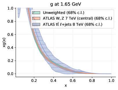
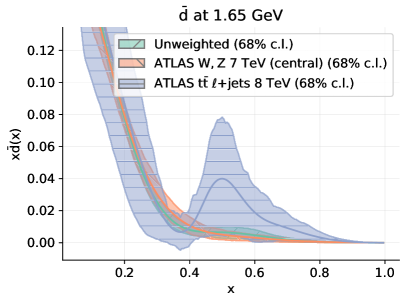
Figure 4.1: The gluon (left) and antidown (right) PDFs at $Q=1.65$ GeV at large $x$, for the unweighted fit and the weighted fits in which the ATLAS $W,Z$ 7 TeV ($\mathcal{L}$=4.6 fb^-1) (central) and the ATLAS $t\bar{t}$ $\ell$+jets 8 TeV datasets are assigned large weight.

Inspection of the PDFs resulting from the weighted fits can provide additional guidance in assessing consistency. This information is used to support, dataset by dataset, the conclusions summarized above. As an example we display the gluon and antidown PDFs in Fig. 4.1. The PDFs are shown at the input scale $Q_{0}=$ 1.65 GeV as a function of $x$ in linear scale for the unweighted fit and for two weighted fits, specifically those in which the ATLAS $W,Z$ 7 TeV ($\mathcal{L}$=4.6 fb^-1) (central) and the ATLAS $t\bar{t}$ $\ell$+jets 8 TeV datasets are assigned large weight. It is clear that for the ATLAS $t\bar{t}$ $\ell$+jets 8 TeV ($1/\sigma d\sigma/dp_{T}^{t}$) data, which are considered inconsistent based on the $\chi^{2}$ analysis, the PDFs in the weighted fit display a significant inflation of PDF uncertainties and an unnatural distortion of the overall PDF shape, including an unphysical valence-like structure of the antidown PDF. Conversely, for the ATLAS $W,Z$ 7 TeV ($\mathcal{L}$=4.6 fb^-1) (central) data, which are considered consistent, the PDFs in the weighted fit have the same shape as the default and only moderately inflated uncertainties. A systematic analysis for all of the weighted fits shows that the behavior of the best fit PDFs confirms the conclusion of the $\chi^{2}$ analysis.

4.3 Choice of jet datasets

As discussed in Sect. 2.2.7, in NNPDF4.0 we consider both single-inclusive jet and dijet production datasets. However the two observables cannot be included simultaneously in the fit because full knowledge of experimental correlations is not available. This also means that we cannot assess their inclusion in the dataset based on weighted fits.

We therefore select the optimal set of jet observables by repeating the analysis carried out in [9]. Specifically, we start from a fit based on the baseline dataset identified above from which we remove all jet measurements. We then compare it to a series of NNLO fits that include, one at a time, the single-inclusive jet or dijet datasets discussed in Sect. 2.2.7, with the theory settings discussed there. The decorrelation model recommended in [88] is used in the case of the ATLAS 8 TeV single-inclusive jet measurement, while systematic uncertainties are decorrelated across rapidity bins in the case of the ATLAS 7 TeV single-inclusive jet measurement.

In Table 4.7 we report the values of the $\chi^{2}$ for all of these fits. Values are shown for all the data grouped by process type and for all single-inclusive jet and dijet data, for both those that are and those that are not included in each fit. The values corresponding to the datasets that are not included in each fit are indicated in square brackets. In Fig. 4.2 we compare the gluon PDF from all the fits, separately for those that include single-inclusive jet or dijet data, at a scale $Q=100$ GeV. The gluon PDF is normalized to the fit that does not include any jet data. We have explicitly checked that all other PDFs are unaffected by the inclusion of jet data.

Dataset	$N_{\rm dat}$	no jets	ATLAS incl. jets 7 TeV, $R=0.6$	CMS incl. jets 7 TeV	ATLAS incl. jets 8 TeV, $R=0.6$	CMS incl. jets 8 TeV	ATLAS dijets 7 TeV, $R=0.6$	CMS dijets 7 TeV	CMS 3D dijets 8 TeV
DIS (fixed-target)	1881	1.06	1.06	1.06	1.07	1.06	1.06	1.06	1.09
DIS (collider)	1208	1.21	1.21	1.21	1.20	1.21	1.21	1.21	1.21
DY (fixed-target)	195	0.98	0.99	0.98	0.99	1.00	0.98	0.99	1.01
$W,Z$ prod. (inclusive)	548	1.34	1.32	1.33	1.36	1.32	1.33	1.34	1.36
$W,Z$ prod. ($p_{T}$ and jets)	150	0.98	0.97	0.97	0.98	1.00	0.96	0.98	0.97
Top pair prod.	66	1.24	1.06	1.16	1.07	1.14	1.11	1.12	1.12
Single-inclusive jets (all)	629	[1.24]	[1.14]	[1.27]	[1.02]	[1.09]	[1.31]	[1.21]	[1.14]
ATLAS incl. jets 7 TeV, $R=0.6$	140	[1.32]	1.26	[1.33]	[1.26]	[1.25]	[1.33]	[1.32]	[1.28]
CMS incl. jets 7 TeV	133	[0.93]	[0.99]	0.86	[0.94]	[1.04]	[0.83]	[0.83]	[0.90]
ATLAS incl. jets 8 TeV, $R=0.6$	171	[1.26]	[1.07]	[1.22]	0.73	[1.01]	[1.10]	[1.09]	[0.65]
CMS incl. jets 8 TeV	185	[1.38]	[1.22]	[1.56]	[1.17]	1.07	[1.82]	[1.51]	[1.65]
Dijets (all)	266	[3.32]	[3.10]	[2.91]	[2.37]	[3.15]	[2.51]	[2.58]	[1.68]
ATLAS dijets 7 TeV, $R=0.6$	90	[2.55]	[2.57]	[2.31]	[2.24]	[2.69]	2.08	[2.22]	[1.91]
CMS dijets 7 TeV	54	[2.60]	[2.62]	[2.33]	[1.99]	[2.58]	[2.20]	2.06	[1.72]
CMS 3D dijets 8 TeV	122	[4.21]	[3.69]	[3.61]	[2.63]	[3.75]	[2.97]	[2.09]	1.50
Isolated $\gamma$ prod.	53	0.72	0.73	0.70	0.73	0.79	0.67	0.71	0.72
Single $t$ prod.	17	0.35	0.36	0.36	0.36	0.36	0.36	0.35	0.38
Total		1.14	1.14	1.13	1.13	1.14	1.16	1.15	1.18

Table 4.7: The $\chi^{2}$ for an NNPDF4.0 variant in which all jet data are excluded, and a series of fits that add to this variant each of the jet measurements of Sect. 2.2.7 one at a time. Results are shown for all datasets, aggregated by process type. For jet data, results are shown both for the sets included in each fit and also for those not included, which are denoted by being enclosed in square brackets. Combined results for all of the jet production data (including data that are and that are not fitted) are also shown. The number of data points in each dataset is also reported.

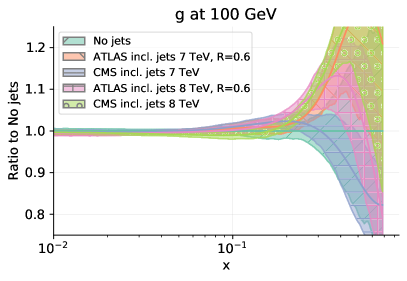
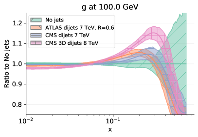
Figure 4.2: The gluon PDF, at $Q=100$ GeV, for some of the fits of Table 4.7: the baseline variant with no jets, and the fits with each of the single-inclusive jet data (left) or each of the dijet data (right). Results are shown normalized to the central value of the no jets variant.

Inspection of Table 4.7 and of Fig. 4.2 leads to the following conclusions.

• All of the 7 TeV data have a rather moderate impact and the global fit quality is essentially unchanged in comparison to the baseline. There is a moderate pull on the large-$x$ gluon, consistent between ATLAS and CMS and between single-inclusive jets and dijets, and also consistent with the baseline within uncertainties.

• The 8 TeV single-inclusive jet data have a moderate pull on the large-$x$ gluon, consistent between ATLAS and CMS, and consistent within uncertainties with the baseline. This pull is in qualitative agreement with but slightly stronger than that of the 7 TeV jet data. The fit quality to all the other data in the global fit is essentially unchanged.

• The only available 8 TeV dijet measurement, from CMS, has a strong pull on the gluon, leading to a result which deviates by about two sigma from the baseline, though the pull is perhaps similar in shape to that of the single-inclusive 8 TeV jet data. The global fit quality deteriorates, but the deterioration is not due to hadron collider data that are sensitive to the gluon, like top and $Z$ $p_{T}$, whose description actually improves, but rather to DIS and DY data.

In general, the 8 TeV ATLAS and CMS single-inclusive jet measurements and the 7 TeV ATLAS and CMS dijet measurements have a very similar effect on the gluon PDF for $x\lesssim 0.2$; dijet datasets seem to suppress the gluon PDF at slightly more moderate value of $x$ than their single-inclusive jet counterparts. This does not seem to affect the description of the rest of the datasets included in the fits.

However, whereas all jet data are broadly consistent with each other, the CMS 8 TeV dijet data are somewhat problematic, as they lead to a gluon that is in disagreement with the baseline in the region around $x\sim 0.3$ and to a visible deterioration in global fit quality. This measurement is peculiar in that it is the only one which is associated to a triple-differential distribution, it leads to the largest reduction of PDF uncertainty, and it is possibly the one that carries most of the experimental information among all of jet measurements. The fact that no corresponding ATLAS measurement is available, and that the global $\chi^{2}$ deteriorates noticeably in comparison to all of the other fits, leads us to conclude that it is more conservative to include the companion single-inclusive jet data in the baseline. For 8 TeV data we thus include in the baseline the single-inclusive jet measurements.

Given the fact that dijet data are preferred on theoretical grounds [137, 213, 9] we include the 7 TeV dijet measurements in the baseline. We will investigate the effect of replacing the 7 TeV ATLAS and CMS dijet measurements with their single-inclusive jet counterparts in Sect. 7.3.3.

5 The NNPDF4.0 parton set

We now present the main result of this work: the NNPDF4.0 parton set. We first discuss fit quality, then present the PDFs, and finally show a comparison of the quality of the fit to a selection of fitted data for a variety of different fits. The NNPDF4.0 PDFs presented here are determined from the baseline dataset of Sect. 4 with the methodology of Sect. 3. We use $\alpha_{s}(m_{Z})=0.118$ at all perturbative orders. All PDF sets are Monte Carlo ensembles of 100 replicas, except in the case of the NNLO NNPDF4.0 baseline, which is a set of 1000 replicas. Additional comparisons, beyond those reported in this section, can be obtained by the reader using the open source NNPDF software framework described in [31], and summarized in Appendix A. For all PDF determinations presented below a last iteration has been performed, in which both the range of the preprocessing exponents (see Sect. 3.1.1) and the $t_{0}$ covariance matrix (recall Sect. 3.2) have been recomputed, and it has been checked explicitly that the results for PDFs are unchanged: this ensures that iterative procedures have achieved convergence.

5.1 Fit quality

Table 5.1 presents an overview of the fit quality for the LO, NLO and NNLO NNPDF4.0 baseline fits. As in previous NNPDF releases, $\chi^{2}$ values are obtained using the published experimental covariance matrix; this is thus not the figure of merit that is minimized in the fit, which is the $\chi^{2}$ computed using the $t_{0}$ covariance matrix (see Ref. [14], specifically Table 9, for a discussion of this issue). The $\chi^{2}$ values that were reported for NNLO PDFs in the NNPDF3.1 analysis of Ref. [5] are also given for comparison.

Datasets are grouped by process type: fixed-target DIS, NC and CC; collider DIS, NC and CC; fixed-target DY; inclusive gauge boson production, separately for the Tevatron and the LHC; LHC gauge boson production with additional jets (including $Z$ $p_{T}$ and $W$+jets); LHC single-inclusive jet and dijet production (for NNPDF3.1 this also includes Tevatron single-inclusive jet production); LHC top pair production; LHC direct photon production; and LHC single top production. The number of data points included in each fit is indicated in parentheses, and $\chi^{2}$ values are provided only for fitted data. A detailed assessment of the compatibility of the NNPDF3.1 PDFs with the full NNPDF4.0 dataset will be presented in Sect. 6.2 below. A graphical representation of the NLO and NNLO values of Table 5.1 is provided in Fig. 5.1.

Dataset	NNPDF4.0						NNPDF3.1
	LO		NLO		NNLO		NNLO
DIS NC (fixed-target)	3.63	(973)	1.40	(973)	1.26	(973)	1.21	(973)
DIS CC (fixed-target)	1.87	(907)	0.87	(907)	0.86	(908)	1.08	(908)
DIS NC (collider)	2.26	(930)	1.18	(980)	1.19	(1127)	1.15	(1130)
DIS CC (collider)	2.48	(81)	1.30	(81)	1.28	(81)	1.18	(81)
Drell-Yan (fixed-target)	0.74	(195)	0.87	(195)	1.00	(195)	1.25	(189)
Tevatron $W,Z$ production (inclusive)	2.11	(64)	1.18	(64)	1.09	(65)	1.29	(74)
LHC $W,Z$ production (inclusive)	7.44	(437)	1.53	(437)	1.37	(483)	1.37	(314)
LHC $W,Z$ production ($p_{T}$ and jets)	4.17	(37)	1.72	(153)	0.98	(150)	1.00	(120)
LHC top-quark pair production	13.4	(66)	1.84	(66)	1.21	(66)	1.08	(19)
LHC jet production	1.95	(500)	1.02	(500)	1.26	(500)	0.94	(470)
LHC isolated $\gamma$ production	9.95	(53)	0.57	(53)	0.77	(53)	—
LHC single $t$ production	0.82	(17)	0.36	(17)	0.36	(17)	—
Total	3.35	(4260)	1.24	(4426)	1.16	(4618)	1.15	(4285)

Table 5.1: Overview of $\chi^{2}$ value by process type for the LO, NLO, and NNLO NNPDF4.0 baseline fits; NNLO NNPDF3.1 is also shown for comparison.

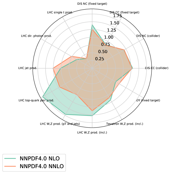
Figure 5.1: Graphical representation of the results of Table 5.1, comparing the $\chi^{2}$ of the NNPDF4.0 NLO and NNLO baseline fits.

Dataset	NNPDF4.0						NNPDF3.1
	LO		NLO		NNLO		NNLO
NMC $F_{2}^{d}/F_{2}^{p}$	0.93	(121)	0.87	(121)	0.87	(121)	0.94	(121)
NMC $\sigma^{{\rm NC},p}$	6.60	(204)	1.82	(204)	1.56	(204)	1.51	(204)
SLAC $F_{2}^{p}$	4.87	(33)	1.67	(33)	0.95	(33)	0.81	(33)
SLAC $F_{2}^{d}$	2.00	(34)	1.01	(34)	0.63	(34)	0.71	(34)
BCDMS $F_{2}^{p}$	3.88	(333)	1.52	(333)	1.41	(333)	1.28	(333)
BCDMS $F_{2}^{d}$	1.76	(248)	1.02	(248)	1.01	(248)	1.11	(248)
CHORUS $\sigma_{CC}^{\nu}$	1.26	(416)	0.96	(416)	0.96	(416)	1.12	(416)
CHORUS $\sigma_{CC}^{\bar{\nu}}$	1.60	(416)	0.90	(416)	0.87	(416)	1.06	(416)
NuTeV $\sigma_{CC}^{\nu}$ (dimuon)	5.54	(39)	0.24	(39)	0.35	(39)	0.60	(39)
NuTeV $\sigma_{CC}^{\bar{\nu}}$ (dimuon)	12.0	(36)	0.43	(36)	0.56	(37)	1.06	(37)
HERA I+II $\sigma_{\rm NC,CC}^{p}$	2.29	(1011)	1.18	(1011)	1.17	(1145)	1.16	(1145)
HERA I+II $\sigma_{\rm NC}^{c}$	—		2.04	(24)	2.03	(37)	1.45	(37)
HERA I+II $\sigma_{\rm NC}^{b}$	—		1.38	(26)	1.43	(26)	1.11	(29)

Table 5.2: Values of the $\chi^{2}$ for each individual experiment included in the NNPDF4.0 PDF determination at LO, NLO, and NNLO; NNPDF3.1 NNLO is also shown for comparison. A dash denotes that the dataset was not included in the specific determination.

Dataset	NNPDF4.0						NNPDF3.1
	LO		NLO		NNLO		NNLO
E866 $\sigma^{d}/2\sigma^{p}$ (NuSea)	0.68	(15)	0.60	(15)	0.49	(15)	0.41	(15)
E866 $\sigma^{p}$ (NuSea)	1.14	(89)	1.30	(89)	1.60	(89)	1.43	(89)
E605 $\sigma^{p}$	0.35	(85)	0.43	(85)	0.46	(85)	1.21	(85)
E906 $\sigma^{d}/2\sigma^{p}$ (SeaQuest)	0.55	(6)	1.28	(6)	0.93	(6)	—

Table 5.3: Same as Table 5.2 for fixed-target DY datasets.

Dataset	NNPDF4.0						NNPDF3.1
	LO		NLO		NNLO		NNLO
CDF $Z$ differential	2.52	(28)	1.27	(28)	1.28	(28)	1.48	(29)
D0 $Z$ differential	1.35	(28)	0.69	(28)	0.64	(28)	0.60	(28)
D0 $W$ electron asymmetry	—		—		—		2.71	(8)
D0 $W$ muon asymmetry	3.31	(8)	2.58	(8)	1.91	(9)	1.56	(9)
ATLAS low-mass DY 7 TeV	4.14	(4)	0.70	(4)	0.88	(6)	0.90	(6)
ATLAS high-mass DY 7 TeV	4.29	(5)	1.82	(5)	1.68	(5)	1.54	(5)
ATLAS $W,Z$ 7 TeV ($\mathcal{L}=35$ pb-1)	3.92	(30)	1.09	(30)	0.98	(30)	0.96	(30)
ATLAS $W,Z$ 7 TeV ($\mathcal{L}=4.6$ fb-1)	17.2	(53)	2.91	(53)	1.67	(61)	2.14	(34)
CMS $W$ electron asymmetry 7 TeV	2.50	(11)	0.92	(11)	0.84	(11)	0.78	(11)
CMS $W$ muon asymmetry 7 TeV	2.10	(11)	1.98	(11)	1.70	(11)	1.75	(11)
CMS DY 2D 7 TeV	4.08	(88)	1.31	(88)	1.36	(110)	1.27	(110)
LHCb $Z\to ee$ 7 TeV	3.38	(9)	1.47	(9)	1.65	(9)	1.48	(9)
LHCb $W,Z\to\mu$ 7 TeV	5.38	(29)	1.59	(29)	1.97	(29)	1.76	(29)
ATLAS low-mass DY 2D 8 TeV	19.4	(47)	1.37	(47)	1.22	(60)	—
ATLAS high-mass DY 2D 8 TeV	5.25	(48)	1.53	(48)	1.11	(48)	—
CMS $W$ rapidity 8 TeV	3.86	(22)	0.93	(22)	1.38	(22)	1.00	(22)
LHCb $Z\to ee$ 8 TeV	6.97	(17)	1.64	(17)	1.33	(17)	1.14	(17)
LHCb $W,Z\to\mu$ 8 TeV	5.37	(29)	1.06	(29)	1.42	(30)	1.37	(30)
ATLAS $\sigma_{W,Z}^{\rm tot}$ 13 TeV	2.69	(3)	0.26	(3)	0.80	(3)	—
LHCb $Z\to ee$ 13 TeV	2.36	(15)	1.70	(15)	1.72	(15)	—
LHCb $Z\to\mu\mu$ 13 TeV	2.85	(16)	1.17	(16)	0.99	(16)	—

Table 5.4: Same as Table 5.2 for inclusive gauge boson production datasets.

Dataset	NNPDF4.0						NNPDF3.1
	LO		NLO		NNLO		NNLO
ATLAS $W^{\pm}+c$ 7 TeV	3.24	(22)	0.61	(22)	—		—
CMS $W^{\pm}+c$ 7 TeV	7.52	(10)	1.42	(10)	—		—
CMS $W^{\pm}+c$ 13 TeV	1.60	(5)	0.74	(5)	—		—
ATLAS $W^{\pm}$+jet 8 TeV	—		1.21	(30)	0.96	(30)	—
ATLAS $Z$ $p_{T}$ 8 TeV ($p_{T},m_{\ell\ell}$)	—		1.11	(40)	0.91	(44)	0.93	(44)
ATLAS $Z$ $p_{T}$ 8 TeV ($p_{T},y_{Z}$)	—		2.78	(18)	0.90	(48)	0.94	(48)
CMS $Z$ $p_{T}$ 8 TeV	—		4.14	(28)	1.41	(28)	1.32	(28)
CMS $\sigma_{tt}^{\rm tot}$ 5 TeV	16.7	(1)	1.95	(1)	0.54	(1)	—
ATLAS $\sigma_{tt}^{\rm tot}$ 7 TeV	117.	(1)	10.3	(1)	4.59	(1)	2.06	(1)
CMS $\sigma_{tt}^{\rm tot}$ 7 TeV	127.	(1)	5.19	(1)	1.06	(1)	0.04	(1)
ATLAS $\sigma_{tt}^{\rm tot}$ 8 TeV	81.9	(1)	1.70	(1)	0.02	(1)	0.27	(1)
CMS $\sigma_{tt}^{\rm tot}$ 8 TeV	119.	(1)	3.43	(1)	0.26	(1)	0.08	(1)
ATLAS $\sigma_{tt}^{\rm tot}$ 13 TeV ($\mathcal{L}$=139 fb-1)	82.7	(1)	3.75	(1)	0.51	(1)	0.01	(1)
CMS $\sigma_{tt}^{\rm tot}$ 13 TeV	52.4	(1)	0.72	(1)	0.06	(1)	0.45	(1)
ATLAS $t\bar{t}~{}\ell$+jets 8 TeV ($1/\sigma d\sigma/dy_{t}$)	7.43	(4)	3.68	(4)	3.22	(4)	1.45	(4)
ATLAS $t\bar{t}~{}\ell$+jets 8 TeV ($1/\sigma d\sigma/dy_{t\bar{t}}$)	17.8	(4)	6.88	(4)	3.77	(4)	—
ATLAS $t\bar{t}~{}2\ell$ 8 TeV ($1/\sigma d\sigma/dy_{t\bar{t}}$)	2.51	(5)	1.85	(5)	1.61	(5)	—
CMS $t\bar{t}~{}\ell$+jets 8 TeV ($1/\sigma d\sigma/dy_{t\bar{t}}$)	4.40	(9)	1.89	(9)	1.23	(9)	0.94	(9)
CMS $t\bar{t}$ 2D $2\ell$ 8 TeV ($1/\sigma d\sigma/dy_{t}dm_{t\bar{t}}$)	2.11	(16)	1.06	(16)	1.03	(16)	—
CMS $t\bar{t}~{}\ell$+jet 13 TeV ($d\sigma/dy_{t}$)	5.50	(11)	0.71	(11)	0.63	(11)	—
CMS $t\bar{t}~{}2\ell$ 13 TeV ($d\sigma/dy_{t}$)	5.47	(10)	0.79	(10)	0.52	(10)	—
CDF incl. jets	—		—		—		0.87	(76)
ATLAS incl. jets 2.76 TeV, $R=0.6$	—		—		—		1.03	(59)
CMS incl. jets 2.76 TeV	—		—		—		1.02	(81)
ATLAS incl. jets 7 TeV, $R=0.6$ (2010)	—		—		—		0.95	(90)
ATLAS incl. jets 7 TeV, $R=0.6$ (2011)	—		—		—		1.07	(31)
CMS incl. jets 7 TeV	—		—		—		0.84	(133)
ATLAS incl. jets 8 TeV, $R=0.6$	1.47	(171)	0.66	(171)	0.69	(171)	—
CMS incl. jets 8 TeV	1.36	(185)	0.96	(185)	1.19	(185)	—
ATLAS dijets 7 TeV, $R=0.6$	3.21	(90)	1.47	(90)	2.15	(90)	—
CMS dijets 7 TeV	3.43	(54)	1.57	(54)	1.81	(54)	—
ATLAS isolated $\gamma$ prod. 13 TeV	9.95	(53)	0.57	(53)	0.77	(53)	—
ATLAS single $t$ $R_{t}$ 7 TeV	0.02	(1)	0.04	(1)	0.50	(1)	—
CMS single $t$ $\sigma_{t}+\sigma_{\bar{t}}$ 7 TeV	6.63	(1)	0.88	(1)	0.73	(1)	—
CMS single $t$ $R_{t}$ 8 TeV	0.01	(1)	0.14	(1)	0.17	(1)	—
ATLAS single $t$ $R_{t}$ 13 TeV	0.22	(1)	0.05	(1)	0.06	(1)	—
CMS single $t$ $R_{t}$ 13 TeV	0.61	(1)	0.33	(1)	0.36	(1)	—
ATLAS single $t$ 7 TeV ($1/\sigma d\sigma/dy_{t}$)	0.52	(3)	0.83	(3)	0.96	(3)	—
ATLAS single $t$ 7 TeV ($1/\sigma d\sigma/dy_{\bar{t}}$)	0.22	(3)	0.06	(3)	0.06	(3)	—
ATLAS single $t$ 8 TeV ($1/\sigma d\sigma/dy_{t}$)	1.13	(3)	0.38	(3)	0.25	(3)	—
ATLAS single $t$ 8 TeV ($1/\sigma d\sigma/dy_{\bar{t}}$)	0.26	(3)	0.19	(3)	0.19	(3)	—

Table 5.5: Same as Table 5.2 for all other LHC datasets.

First, one can observe how fit quality markedly improves with perturbative order: the $\chi^{2}$ decreases from 3.35 at LO to 1.24 at NLO and 1.16 at NNLO. The significant improvement in fit quality from NLO to NNLO was already reported in NNPDF3.1 (see specifically Sect. 3.2 in [5]) and it is chiefly due to the large number of high-precision LHC data, for which the $\chi^{2}$ improves most: specifically gauge boson and top pair production. Fit quality is generally good: specifically, both the value of $\chi^{2}$ and the value of $n_{\sigma}$ Eq. (4.3) corresponding to the global fit are similar to those of other recent global PDF determinations CT18 [143] and MSHT20 [144], despite the fact that this PDF determination includes a larger number of datapoints and of different processes. Of course, comparison of $\chi^{2}$ values between different PDF sets should be taken with care, given differences in dataset and theory settings: the recent PDF4LHC study [214, 215] has shown that fit quality in NNPDF3.1 is similar to that of CT18 and MSHT20. The largest $\chi^{2}$ value ($\chi^{2}=1.37$) is found for LHC inclusive gauge boson production, which has by far the highest precision. The opposite extreme is single top datasets, which have relatively low precision and a very low $\chi^{2}$ value.

The quality of the NNLO NNPDF4.0 fit is comparable to that of its NNPDF3.1 counterpart. This is especially remarkable in view of the substantial extension of the dataset from NNPDF3.1 to NNPDF4.0. A comparative analysis of the impact of different data and an assessment of the role played by the methodology will be respectively presented in Sect. 7 and Sect. 8 below. Specifically, we will see that a NNLO fit to the NNPDF3.1-like dataset (see Sect. 7.1.1 below) leads to $\chi^{2}=1.145$ if NNPDF4.0 methodology is used, while the significantly worse value $\chi^{2}=1.186$ is found using NNPDF3.1 methodology.

In Tables 5.2-5.5 we provide the details of the $\chi^{2}$ value for each dataset included in each PDF determination. We make the following observations.

• The impact of NNLO QCD corrections is apparent for several of the LHC datasets, in particular for $Z$ $p_{T}$ and top pair production, whose $\chi^{2}$ improves significantly when moving from NLO to NNLO.

• Fit quality at NNLO is good and uniform across different datasets, with variations compatible with statistical fluctuations.

• A good description of the inclusive gauge boson production data is achieved, irrespective of the kinematic region probed by specific datasets, despite their extremely high precision.

• Measurements with poor fit quality are those already singled out in Sect. 4 that have been retained for the reasons explained there: specifically the combined HERA charm cross section, the D0 muon asymmetry, the LHC $W,Z\to\mu$ 7 TeV rapidity distributions and the ATLAS top pair 8 TeV rapidity distributions in the lepton+jet final state and 7 TeV total cross-section. For some of these, fit quality is somewhat worse in NNPDF4.0 than NNPDF3.1, due to the larger number of competing datasets included in the NNPDF4.0 determination. We have checked explicitly that if we exclude in turn experiments with the worse fit quality, and we combine the ensuing replicas into a single set, we obtain results that are compatible within statistical fluctuations with those of the default global fit.

5.2 Parton distributions

We now examine the baseline NNPDF4.0 parton distributions. We first show the full set of PDFs, compared to their NNPDF3.1 predecessors. We then discuss sources of theoretical uncertainties: the dependence on the perturbative order and on the value of the strong coupling. We finally compare the NNLO NNPDF4.0 baseline PDFs to CT18 [143] and MSHT20 [144]. A further comparison with these PDF sets in terms of phenomenology, i.e. specifically for parton luminosities and theoretical predictions for LHC observables, will be presented in Sect. 9.

5.2.1 Comparison to NNPDF3.1

The full set of NNLO NNPDF4.0 and NNPDF3.1 PDFs are shown in Fig. 5.2, and the associated relative one-sigma uncertainties are displayed in Fig. 5.3. Specifically, we show the up, antiup, down, antidown, strange, antistrange, charm and gluon PDFs as a function of $x$ at $Q=100$ GeV. Results are normalized to the NNPDF4.0 central value.

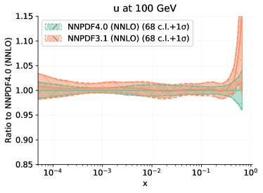
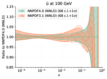
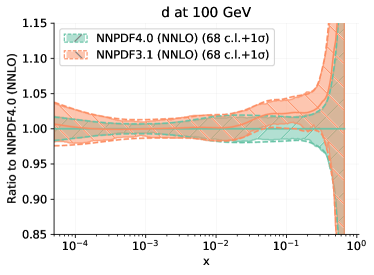
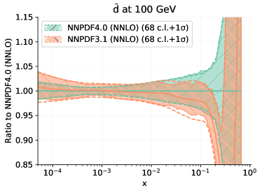
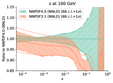
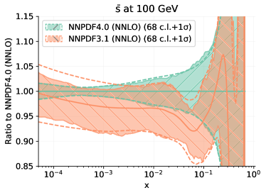
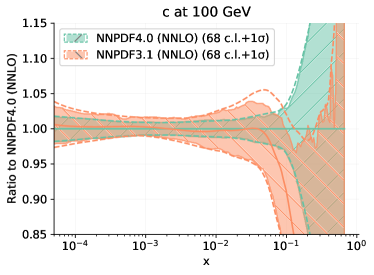
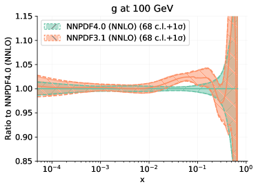
Figure 5.2: The full set of NNLO NNPDF4.0 PDFs: the up, antiup, down, antidown, strange, antistrange, charm and gluon PDFs at $Q=100$ GeV, compared to NNPDF3.1. Results are normalized to the central NNPDF4.0 value. Solid and dashed bands correspond to 68% c. l. and one-sigma uncertainties, respectively.

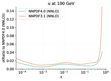
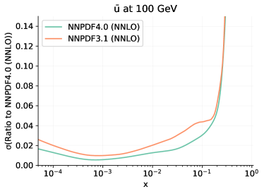
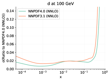
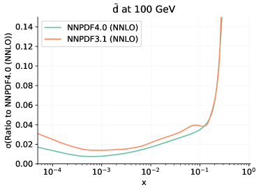
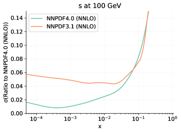
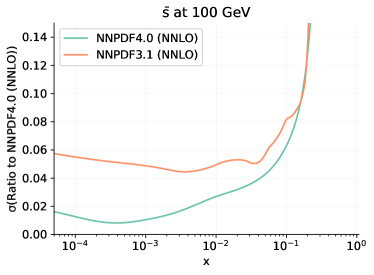
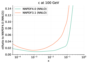
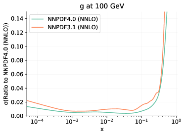
Figure 5.3: Same as Fig. 5.2 but for one-sigma relative uncertainties.

There is remarkable consistency between the new NNPDF4.0 PDF set and the previous NNPDF3.1 analysis. The only noticeable differences appear in the strange and antistrange PDFs and in the gluon. As we shall show in Sect. 7.1, in the former case this is mainly due to the inclusion of NNLO corrections in the treatment of the NuTeV data (see Sect. 2.1): indeed, this same effect was already observed in a recent dedicated study of strangeness [10]. In the latter case, the difference, i.e. the suppression of the gluon around $x\sim 0.1$, is mainly due to the extra physical constraints provided by additional single-inclusive jet, dijet and top pair measurements included in NNPDF4.0, see also the discussion of Sect. 7.

The precision of the PDFs in the NNPDF4.0 set increases significantly in comparison to NNPDF3.1. Depending on the kinematic region and on the parton, the reduction of the PDF relative uncertainty ranges from 30% to more than 50%. The relative uncertainty of almost all of the NNPDF4.0 PDFs is of the order of 1-2% in the region probed by experimental data. In Sects. 7 and  8 we will disentangle how much of this reduction is due to the improved fitting methodology and how much to the extended dataset.

5.2.2 Dependence on the perturbative order and on the strong coupling

In Fig. 5.4 the up, antiup, charm and gluon NNPDF4.0 PDFs are compared for the three perturbative orders, LO, NLO and NNLO, as a function of $x$ at $Q=100$ GeV. Results are normalized to the central value of the NNLO set. As expected, a large shift is observed from LO to NLO due to the large NLO corrections, as is also clear from the poor quality of the LO fit seen in Tabs. 5.1-5.5. This is consistent with previous NNPDF studies.

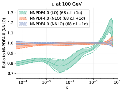
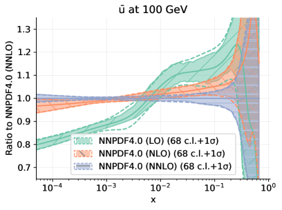
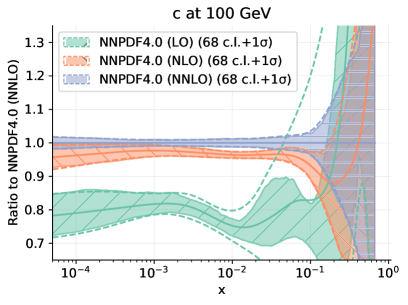
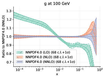
Figure 5.4: Comparison between the LO, NLO and NNLO NNPDF4.0 PDFs. The up, antiup, charm and gluon are shown at $Q=100$ GeV. All results are normalized to the central value of the NNLO set. Solid and dashed bands correspond respectively to 68% c. l. and one-sigma uncertainties.

However, the difference between NLO and NNLO PDFs is also noticeable. While the NLO and NNLO PDFs are very compatible within uncertainties for the up quark, in the case of the charm quark PDF at intermediate values of $x$ and in the case of the gluon PDF at large values of $x$ the shift in central value is comparable or even somewhat larger than the uncertainty band. This means that at NLO the missing higher order uncertainty is no longer negligible in comparison to the PDF uncertainty, unlike in previous PDF determinations, including NNPDF3.1 (see Fig. 3.12 in [5]), where NLO and NNLO PDFs generally agreed within their larger errors. Interestingly, the shift in central value in the NLO PDFs observed in Refs. [23, 24] when missing higher order corrections are added during the fit seems to be of the same size and sign as the shift between NLO and NNLO results seen in Fig. 5.4. This suggests that the inclusion of the missing higher order uncertainty along the lines of Refs. [23, 24] would be highly desirable also at NNLO.

An important source of theory uncertainty that is routinely included is that related to the variation of $\alpha_{s}$. The default value of the strong coupling adopted for NNPDF4.0 at all perturbative orders is $\alpha_{s}(m_{Z})=0.118$, in agreement with the latest PDG value of $\alpha_{s}(m_{Z})=0.1179\pm 0.0010$ [141]. In order to properly include correlated PDF+$\alpha_{s}$ uncertainties [216] in the computation of LHC observables, we also provide sets corresponding to different values of $\alpha_{s}$. Specifically, we provide PDFs obtained with $\alpha_{s}(m_{Z})=0.116,\,0.117,\,0.1175,\,0.1185,\,0.119,\,0.120$. They are shown in Fig. 5.5, along with the baseline, normalized to the central value of the latter. Only the change in central value is shown: relative PDF uncertainties are essentially unchanged when $\alpha_{s}$ is varied. Note that the change in central value as $\alpha_{s}$ is varied by one-sigma is smaller or much smaller than the PDF uncertainty. Of course, the gluon displays the strongest dependence on $\alpha_{s}$, and it decreases at small $x$ and increases at large $x$ as the value of $\alpha_{s}$ is increased.

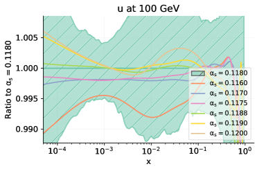
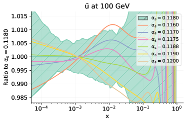
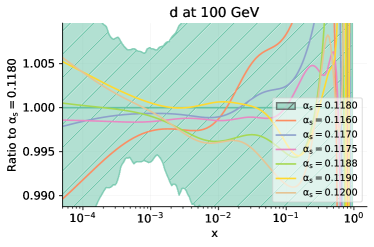
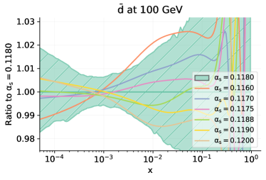
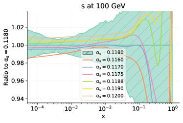
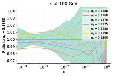
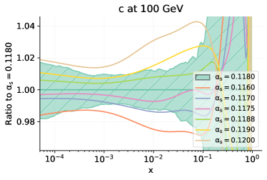
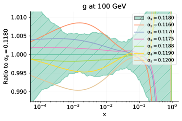
Figure 5.5: Same as Fig. 5.2, now comparing PDFs obtained using different values of $\alpha_{s}(m_{Z})=0.116,\,0.117,\,0.1175,\,0.118,\,0.1185,\,0.119,\,0.120$, normalized to the $\alpha_{s}(m_{Z})=0.118$ baseline, with only the central value shown for other sets.

In Table 5.6 we show the value of the $\chi^{2}$ per data point obtained in the NNLO fit corresponding to each value of $\alpha_{s}$. Whereas a full determination of $\alpha_{s}$ should be done [206] by using the correlated replica method of Ref. [138], and also including theory uncertainties, these values suggest that the best-fit value of $\alpha_{s}$ within the NNPDF4.0 framework is consistent with the NNPDF3.1-based determination of Ref. [206] and with the current PDG value.

$\alpha_{s}(m_{Z})$	0.1160	0.1170	0.1175	0.1180	0.1185	0.1900	0.1200
$\chi^{2}$	1.183	1.169	1.165	1.162	1.161	1.162	1.168

Table 5.6: Values of the total $\chi^{2}$ per data point for the NNLO global fit with different values of $\alpha_{s}(m_{Z})$.

As already discussed in Ref. [5], the remaining parametric uncertainties, related to the values of the quark masses, are expected to be very small, since the dependence on the charm mass is almost entirely removed by parametrizing the charm PDF, and the dependence on the bottom quark mass is very small (except on the $b$-PDF itself and processes specifically sensitive to it).

5.2.3 Comparison to other PDF sets

The NNPDF4.0 NNLO PDFs are compared to other recent global sets, namely CT18 [143] and MSHT20 [144], in Fig. 5.6. Note that there are substantial differences in the underlying dataset: the CT18 dataset is very close to that of NNPDF3.1 while the MSHT20 dataset is somewhere in between NNPDF3.1 and NNPDF4.0 (see Appendix. B for a detailed comparison). All results are shown at $Q=100$ GeV, normalized to the central NNPDF4.0 value. Relative uncertainties are compared in Fig. 5.7. Note that while for NNPDF4.0 there are eight independently parametrized PDFs, for CT18 the strange and antistrange are not independently parametrized, and for both CT18 and MSHT20 charm is not independently parametrized.

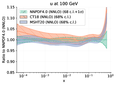
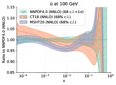
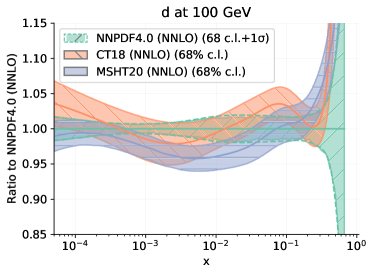
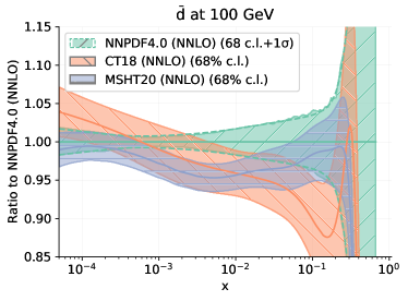
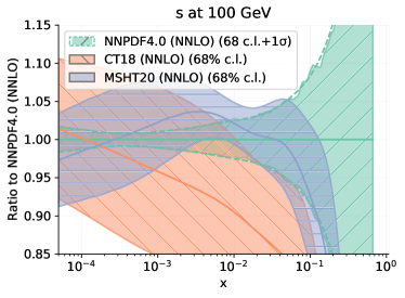
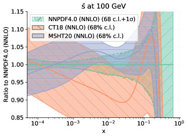
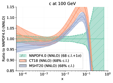
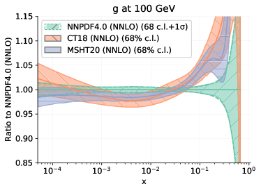
Figure 5.6: Comparison between the NNPDF4.0, CT18 and the MSHT20 NNLO PDF sets. The up, antiup, down, antidown, strange, antistrange, charm and gluon PDFs are shown at $Q=100$ GeV, normalized to the central NNPDF4.0 value. For NNPDF4.0, solid and dashed bands correspond respectively to 68% c. l. and one-sigma uncertainties.

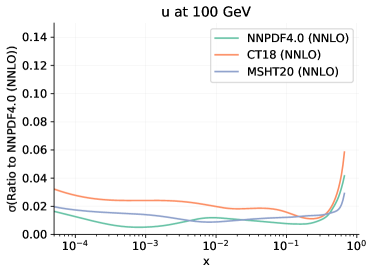
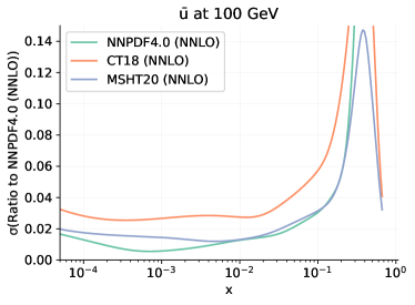
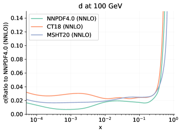
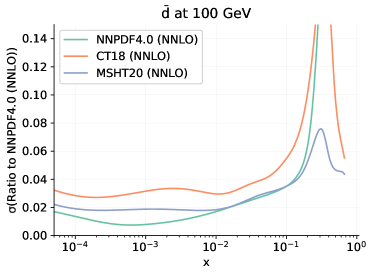
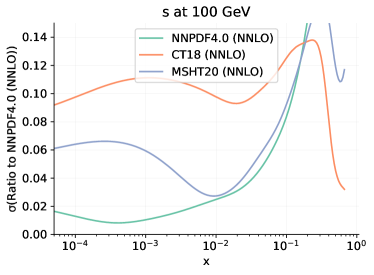
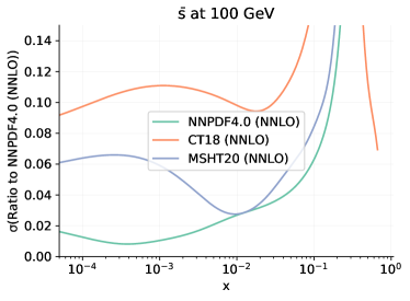
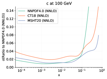
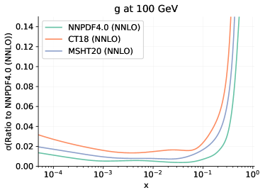
Figure 5.7: Same as Fig. 5.6 but for one-sigma relative uncertainties.

The three parton sets are overall in fair agreement within their respective uncertainties, though some differences in shape are observed. Interestingly, these follow the pattern already observed in [5] when comparing NNPDF3.1 [5] to CT14 [217] and MMHT2014 [218] (see in particular Fig. 12 in Ref. [5]) . The up and down PDFs are in good agreement, in particular the NNPDF4.0 result is always within the envelope of the CT18 and MSHT20 uncertainties. More marked differences are observed for the antiup and antidown PDFs: note, however, that the CT18 and MSHT20 PDF sets do not include the E906/SeaQuest and the LHCb 13 TeV measurements, which provide additional constraints on sea quark flavor separation at mid- and large-$x$ values, as discussed in Sect. 7 (see Ref. [212] for a discussion of the SeaQuest data in the CT18 framework). The NNPDF4.0 strange and antistrange PDFs agree very well with MSHT20: in both these PDF sets, strangeness is enhanced in comparison to CT18. As suggested in [144, 10], this is likely due to the fact that the ATLAS $W,Z$ 7 TeV data are not included in the default CT18 fit (though they are included in the CT18A variant set), and that NNLO massive corrections to the neutrino DIS dimuon cross-sections are also not accounted for.

The NNPDF4.0 charm PDF is suppressed at intermediate values of $x$ in comparison to CT18 and MSHT20, as a consequence of the fact that charm in CT18 and MSHT20 is determined by perturbative matching conditions and is not independently parametrized. The gluon is in fair agreement in the region of $x\lesssim 0.03$ which is relevant for Higgs production though the NNPDF result is at the upper edge of the MSHT20 and CT18 uncertainty; this was already the case when comparing NNPDF3.1 to CT14 and MMHT2014. At larger values of $x$, the NNPDF4.0 gluon is suppressed in comparison to CT18 and MSHT20. This behavior is likely due to the LHC top pair and jet data that are included in NNPDF4.0 but not in the other sets.

Concerning the associated PDF uncertainties, NNPDF is generally more precise, while CT18 has generally larger uncertainties. This is consistent with the observation that CT18 is based on a somewhat smaller dataset than NNPDF4.0, with MSHT20 being in between, see Appendix B for more details.

5.3 Comparison to experimental data

In Fig. 5.8 we present for illustrative purposes a comparison between a selection of data included in the NNPDF4.0 baseline fits and the corresponding NLO and NNLO best-fit results, with the main goal of providing a visual assessment of the fit quality and of the relative size of the data and PDF uncertainties. The data shown are selected as representative of the global dataset; specifically we show results for the following data: the lowest $Q$ bin of the combined HERA charm cross-section [145]; the SeaQuest (DYE906) differential cross section [117]; the central rapidity bin of the ATLAS 7 TeV $W^{+}$ rapidity distribution [54]; the highest dilepton invariant mass bin for ATLAS 8 TeV high-mass DY [79]; the $0.5\leq|y|\leq 1.0$ dijet rapidity bin for the CMS 7 TeV dijets [76]; the lowest $p_{T}^{Z}$ bin of the CMS 8 TeV $Z$ $p_{T}$ distribution [66]; the ATLAS 8 TeV normalized single top rapidity distribution [98]; and the top rapidity distribution for CMS 13 TeV top pairs in the lepton+jets final state [93]. All results are normalized to the central experimental value. Data error bars correspond to the sum in quadrature of all uncertainties. Correlated systematic uncertainties are large or even dominant in several cases, therefore the plots displayed in Fig. 5.8 should be viewed as a qualitative indication, while a quantitative assessment is provided by the $\chi^{2}$ values of Tables 5.2-5.5. A full set of comparisons of the NNLO PDF to all the data included in the fit are linked to the NNPDF website https://nnpdf.mi.infn.it/nnpdf4-0/ and can be found in [219].

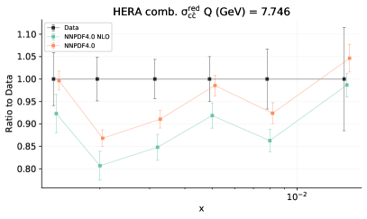
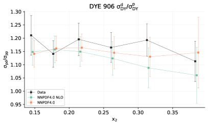
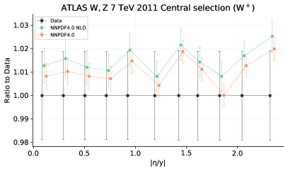
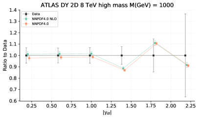
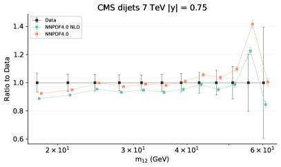
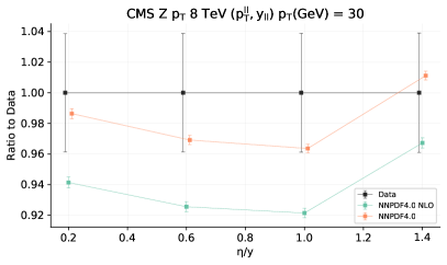
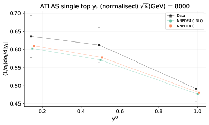
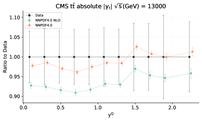
Figure 5.8: Comparison between data points and NLO and NNLO best-fit results for a selection of fitted data points (see text). Results are shown as ratios to the central experimental value, with one-sigma experimental and PDF uncertainties. The experimental uncertainty is the sum in quadrature of all statistical and systematic uncertainties.

It is clear that NNLO corrections are significant in many cases as already noticed: specifically for combined HERA charm, SeaQuest, the CMS 7 TeV dijets, CMS 8 TeV $Z$ $p_{T}$ and the CMS 13 TeV top pairs. In all these cases, the quality of the best fit visibly improves at NNLO. PDF uncertainties are generally smaller than data uncertainties. This is in part due to the fact that experimental uncertainties are correlated while the diagonal uncertainty is shown in the plots, but also to the fact that PDFs are simultaneously constrained by several datasets. Indeed, PDF uncertainties become comparable to data uncertainties when the data shown are the only ones to constrain the relevant PDFs: an example is the SeaQuest data at very large $x_{2}$ (momentum fraction of the struck parton), which is essentially the only dataset that constrains the $\bar{d}/\bar{u}$ ratio in this region.

6 Validation of the methodology

We perform here a detailed validation of the NNPDF4.0 fitting methodology, with the main goal of verifying that the resulting PDF uncertainties have been faithfully estimated. A validation technique through closure tests was introduced by us in Ref. [14], in order to validate the NNPDF3.x methodology. This technique checks for the faithfulness of PDF uncertainties in the region in which PDFs are constrained by the data. We will apply it systematically to NNPDF4.0 in Sect. 6.1.1: thanks to the greater computational efficiency of the NNPDF4.0 methodology (see Sect. 3.4) we can now perform much more extensive and systematic tests than was previously possible. Furthermore, we can now also test for faithfulness of uncertainties in the extrapolation region, i.e. where PDFs are not directly constrained by data, by means of future tests, introduced recently in Ref. [15]. Future tests of the NNPDF4.0 methodology will be presented in Sect. 6.2. This extensive validation, both in the data and the extrapolation regions, is especially desirable given the small, percent-level PDF uncertainties that NNPDF4.0 achieves.

6.1 Closure testing NNPDF4.0

The closure testing methodology was introduced for global PDF fits in Ref. [14], following a suggestion in Ref. [220] and previous studies in Ref. [221]. Here we follow the original approach of Ref. [14] and supplement it with a wider variety of estimators and more systematic studies. First, we review the closure testing methodology and describe the settings adopted for the closure tests of NNPDF4.0. Then we introduce the statistical estimators used to validate the outcome of these tests, including the definition of some new estimators. Finally, we present a detailed closure test analysis of the NNPDF4.0 methodology, based on the statistical estimators introduced previously. A discussion of the limitations of the closure tesing methdology is also given in conclusion. A more detailed theoretical discussion of the statistical underpinnings of the closure testing methodology that we adopt can be found in Ref. [222].

6.1.1 The closure test setup

The basic idea of closure testing is to perform a PDF determination based on artificial data that have been generated with perfect statistical properties from a known underlying law. Comparing results to the known truth then allows one to check for statistical consistency.

Specifically, assume that we have $N_{\rm dat}$ experimental measurements, normally distributed around the true values $\boldsymbol{f}$ with covariance matrix $C$. The central values of the experimental data $\boldsymbol{z}$ will then be given in terms of their true values as

$$z_{i}=f_{i}+\eta_{i}\,,\quad i=1\,\ldots,N_{\rm dat}\,,$$ (6.1)

where the vector of shifts $\boldsymbol{\eta}$ is drawn from a multi-Gaussian distribution with covariance $C$, $\mathcal{N}(\boldsymbol{0},C)$. Within the Monte Carlo replica method for error propagation adopted in this work, the pseudodata which are used as actual input for the PDF fit, $\boldsymbol{y}^{(k)}$, are generated by adding a further layer of fluctuations,

$$y^{(k)}_{i}=f_{i}+\eta_{i}+\epsilon^{(k)}_{i}\,,\quad i=1\,\ldots,N_{\rm dat}\,,\quad k=1\,\ldots,n_{\rm rep}\,,$$ (6.2)

where the index $k$ indicates that each Monte Carlo replica is generated by drawing an independent noise vector $\boldsymbol{\epsilon}$ from the same multi-Gaussian distribution $\mathcal{N}(\boldsymbol{0},C)$. In the NNPDF approach, for each Monte Carlo replica $k$ defined in Eq. (6.2) a neural network such as that displayed in Fig. 3.9 is trained from the minimization of a figure of merit, see also the discussion in Sect. 3. This means that the neural network parameters are chosen by optimizing

$$E^{(k)}={{1}\over{N_{\rm dat}}}\sum_{ij}(g^{(k)}_{i}-y^{(k)}_{i})C^{-1}_{ij}(g^{(k)}_{j}-y^{(k)}_{j})\,,$$ (6.3)

where we denote by $\boldsymbol{g}^{(k)}$ the predictions for the experimental data obtained from the neural network model fitted to the $k$-th replica.

In a fit to actual experimental data we have access to the measured central values $\boldsymbol{z}$ and to the covariance matrix $C$ as estimated by the experimentalists. In a closure test we instead use a given set of PDFs and associated theoretical calculation as input for the central values. Hence, the starting point of the closure test is a known proxy of the true underlying observable values, $\boldsymbol{f}$. Subsequently, a proxy for the experimental central values is generated following Eq. (6.1). A closure test thus amounts to applying to closure test data the NNPDF methodology as it would be used in a fit to actual experimental data.

6.1.2 Statistical estimators

A successful closure test must be such that the resulting PDF fit yields a faithful statistical description of the known underlying law. In order to assess quantitatively the degree of success of the NNPDF4.0 closure tests presented here, we have extended and systematized the set of estimators introduced in previous studies [14]. Here we provide a summary of the estimators and their justification; for more detailed derivations and arguments showing of how they fit into a Bayesian approach to inverse problems we refer the reader to [222].

Bias, variance, and noise in closure tests.

We define an error function as the expectation value across PDF replicas, denoted as $\mathbf{E}_{\epsilon}\left[\cdot\right]$, of the $\chi^{2}$ evaluated between the data predictions obtained from the $k$-th PDF replica, $\boldsymbol{g}$, and the corresponding experimental central values, $\boldsymbol{z}$,

$$\mathbf{E}_{\epsilon}\left[{\chi^{2}}^{(k)}\right]\equiv{{1}\over{N_{\rm dat}}}\mathbf{E}_{\epsilon}\left[\sum_{ij}(g^{(k)}_{i}-z_{i})C^{-1}_{ij}(g^{(k)}_{j}-z_{j})\right]\,.$$ (6.4)

It is easy to check [222] that this expression can be decomposed as

$$\begin{split}\mathbf{E}_{\epsilon}\left[{\chi^{2}}^{(k)}\right]&={\rm noise}+{\rm bias}+{\rm variance}-{\rm cross\,term}\\ &={\rm noise}+{\rm variance}+\Delta_{\chi^{2}},\\ &=\chi^{2}+{\rm variance}\,,\end{split}$$ (6.5)

where each of the quantities on the right-hand side is defined as follows.

First of all, the noise is defined as

$$\mathrm{noise}={{1}\over{N_{\rm dat}}}\sum_{ij}\left(f_{i}-z_{i}\right)C^{-1}_{ij}\left(f_{j}-z_{j}\right)$$ (6.6)

and represents the fluctuations of the experimental data $\boldsymbol{z}$ around the true value $\boldsymbol{f}$. Eq. (6.6) is clearly independent of the model adopted, being an intrinsic property of the experimental measurements. Note that by construction the noise will tend to one in the limit of large $N_{\rm dat}$.

The bias is defined as the difference between the central value of the model replica predictions, $\mathbf{E}_{\epsilon}\left[g\right]$, and the true observable values $\boldsymbol{f}$, in units of the experimental covariance matrix, i.e.

$${\rm bias}={{1}\over{N_{\rm dat}}}\sum_{ij}\left(\mathbf{E}_{\epsilon}\left[g\right]-f\right)_{i}C^{-1}_{ij}\left(\mathbf{E}_{\epsilon}\left[g\right]-f\right)_{j}\,.$$ (6.7)

The bias measures the deviation between the result of the fit and the underlying law. In general, it is desirable for a PDF fit to exhibit a smaller bias because that indicates that the fit results are closer to the truth. However, consistency of a PDF fit does not depend on the size of the bias, but rather, on whether the size of the bias is correctly reproduced by the PDF uncertainty, as we discuss below.

Finally, the variance term describes the fluctuations of the model replica predictions around their mean value again in units of the experimental covariance matrix,

$${\rm variance}={{1}\over{N_{\rm dat}}}\mathbf{E}_{\epsilon}\left[\sum_{ij}\left(\mathbf{E}_{\epsilon}\left[g\right]-g^{(k)}\right)_{i}C^{-1}_{ij}\left(\mathbf{E}_{\epsilon}\left[g\right]-g^{(k)}\right)_{j}\right]\,,$$ (6.8)

which can be interpreted as the projection of the PDF uncertainty to the space of experimental data. We note that this variance as defined in Eq. (6.8) actually corresponds to the square of the estimator $\phi$ introduced in [14]. For a discussion of the cross term in Eq. (6.5) we refer to [222].

Since the variance can be determined purely from the model predictions and the experimental covariance matrix, it can also be calculated for fits to real experimental data. This is in contrast to the noise Eq. (6.6) and bias Eq. (6.7), which depend on the true law $\boldsymbol{f}$ and hence can only be evaluated in closure tests. It is also important to note here that both variance and bias can be computed without using any knowledge of statistical fluctuations that enter closure tests.

One can observe that the second line of the decomposition of the error function in Eq. (6.5) is expressed as the sum of the noise, the variance, and of $\Delta_{\chi^{2}}$. This last quantity was introduced in [14] and is defined as the difference between the $\chi^{2}$ evaluated from comparing the expectation value of the model predictions $\mathbf{E}_{\epsilon}\left[g\right]$ and the level one data $\boldsymbol{z}$, that is $\chi^{2}\left[\mathbf{E}_{\epsilon}\left[\boldsymbol{g}\right],\boldsymbol{z}\right]$, and the $\chi^{2}$ evaluated between the underlying observable values $\boldsymbol{f}$ and the same level one data, that is $\chi^{2}\left[\boldsymbol{f},\boldsymbol{z}\right]$. We note that the latter coincides with the noise in Eq. (6.6). Here we slightly redefine $\Delta_{\chi^{2}}$ as compared to [14] by normalizing by the number of data points, such that

$$\begin{split}\Delta_{\chi^{2}}&\equiv\chi^{2}\left[\mathbf{E}_{\epsilon}\left[\boldsymbol{g}\right],\boldsymbol{z}\right]-\chi^{2}\left[\boldsymbol{f},\boldsymbol{z}\right]\\ &=\chi^{2}-{\rm noise}\,.\end{split}$$ (6.9)

With this definition, constant values of $\Delta_{\chi^{2}}$ define elliptical contours in data space centered on the pseudodata Eq. (6.1).

The value of $\Delta_{\chi^{2}}$ can be interpreted as a qualitative measure of over- or under-fitting, when it is evaluated on data included in the fit. In particular, $\Delta_{\chi^{2}}=0$ defines a contour which is centered on the fitted level one data and passes through the underlying observables. If $\Delta_{\chi^{2}}<0$ then the expectation value of the model predictions fit the level one data better than the underlying observables: this then suggests an overfitting of the shift $\boldsymbol{\eta}$. Similarly, $\Delta_{\chi^{2}}>0$ indicates underfitting of the level one data. As discussed in Ref. [222] however, the replica distribution can be perfectly sampled from the posterior distribution in model space and $\Delta_{\chi^{2}}$ can still be negative. The overall shift of the PDF predictions is thus not an issue as long as the uncertainties account for it. The bottom line is that finding values of $\Delta_{\chi^{2}}\leq 0$ in the closure test remains acceptable provided their magnitude is sufficiently small, which would indicate some combination of a smaller correlation with the level one data and a smaller bias. Assuming that in such a case one finds that the PDF uncertainties are faithful, this result can be interpreted as passing the closure test.

In summary, the closure tests provide us with indicators that allow us to assess whether PDF uncertainties are faithful, and furthermore how close the fit is to the truth, i.e. whether the final result is optimal fit, or an over- or under-fit. This provides a criterion for comparing methodologies: given two methodologies that both produce a faithful result, an over- or under-fitted methodology is disfavored in comparison to one that leads to a proper fit. We now turn to our main indicator for faithfulness, the bias-to-variance ratio.

The bias-to-variance ratio for closure tests.

In the context of a closure test fit, the experimental central values (or level one data) defined in Eq. (6.1) are viewed as stochastic variables. When one performs fits to experimental data, $\boldsymbol{z}$ is fixed at the published central value which will be to some extent shifted from the true observable value due to the experimental uncertainties. However, in closure fits we are free to generate several instances of the shift $\boldsymbol{\eta}$, and use this feature to design our estimators — these would correspond to “runs of the universe” in the real world.

Considering the data which are included in the fit, the bias Eq. (6.7) is potentially driven by two methodology related features which we are aiming to validate with the closure test. The first mechanism is broadly described as under-fitting, and covers inflexibility of the model or inability for the optimization algorithm to sufficiently minimize the cost function. The second mechanism would be over-fitting of the level one shift, which means that the central value of the observables is systematically shifted towards the level one data by an amount that is not properly accounted for by the PDF uncertainties, which are thus underestimated. Note that in order for the testing of these effects to be nontrivial it is necessary to select the underlying truth as sufficiently flexible and in a model-independent way.

Due to its dependence on the shift vector, $\boldsymbol{\eta}$, $\Delta_{\chi^{2}}$ is a stochastic variable. In order to characterize the regime our model is in, we need to understand its probability distribution, rather than computing a single instance of it. For this purpose, we run multiple closure fits, each time with different shifts; we then reconstruct the distribution, and determine the expectation value of $\Delta_{\chi^{2}}$ across fits. It is worth noting that, compared to previous NNPDF studies, a study using multiple full replica closure fits has only been made possible by the computational speed up from deployment of state-of-the-art machine learning algorithms detailed in Sec. 3. Results for the distribution of the $\Delta_{\chi^{2}}$ estimator over fits are presented in Sect. 6.1.4.

The main question to be addressed by the closure test is whether the uncertainty of the PDFs, represented by an ensemble of PDF replicas, is a faithful propagation of the data uncertainty into the space of PDFs. In the context of running multiple closure fits this question can be answered either by looking at the PDFs directly (as was done in Ref. [14]), or by looking at predictions for physical observables obtained using these PDFs. The latter choice offers the distinct advantage that the space of physical observables always has a finite dimension, equal to the number of data points for which predictions are computed. In order for the test to be nontrivial, we choose to evaluate the estimators on data which were not included in the fit, so that we are assessing whether uncertainties are faithful on new observables.

From a Bayesian perspective, the PDF replicas obtained from a fit to a given set of data can be treated as a sample from the prior model distribution for data which was not used in that fit, similarly to the concept of Bayesian reweighting [155, 156]. For the present study, we will perform fits on a subset of the full NNPDF4.0 dataset and then calculate the estimators discussed below on some test data which were not included in each fit.

In order to evaluate the faithfulness of the PDF uncertainties, one can first take the expectation of the bias across fits with different shifts in Eq. (6.1), namely

$$\begin{split}\mathbf{E}_{\eta}\left[{\rm bias}\right]&={{1}\over{N_{\rm dat}}}\mathbf{E}_{\eta}\left[\sum_{ij}\left(\mathbf{E}_{\epsilon}\left[g\right]-f\right)_{i}C^{-1}_{ij}\left(\mathbf{E}_{\epsilon}\left[g\right]-f\right)_{j}\right]\\ &={{1}\over{N_{\rm dat}}}\mathrm{tr}\left(\Sigma^{\rm bias}C^{-1}\right),\end{split}$$ (6.10)

where the subindex $\mathbf{E}_{\eta}\left[.\right]$ indicates that we are averaging over fits with different level-one shifts $\boldsymbol{\eta}$. In Eq. (6.10) we introduced $\Sigma^{\rm bias}$, the covariance matrix of the difference between the central value of the predictions and the true observable values estimated from the sample of fits,

$$\Sigma^{\rm bias}\equiv\mathbf{E}_{\eta}\left[\left(\mathbf{E}_{\epsilon}\left[g\right]-f\right)\left(\mathbf{E}_{\epsilon}\left[g\right]-f\right)^{T}\right]\,.$$ (6.11)

The expectation of the bias across fits is then the expected distance between the central predictions and the true values in units of the covariance matrix averaged across all data. If the fluctuations over fits reproduce the experimental covariance $C$ exactly, then the estimator defined in Eq. (6.10) should be equal to one.

Similarly, we can take the expectation value of the variance across fits with different shifts Eq. (6.1),

$$\begin{split}\mathbf{E}_{\eta}\left[{\rm variance}\right]&={{1}\over{N_{\rm dat}}}\mathbf{E}_{\eta}\left[\mathbf{E}_{\epsilon}\left[\sum_{ij}\left(\mathbf{E}_{\epsilon}\left[g\right]-g^{(k)}\right)_{i}C^{-1}_{ij}\left(\mathbf{E}_{\epsilon}\left[g\right]-g^{(k)}\right)_{j}\right]\right]\\ &={{1}\over{N_{\rm dat}}}\mathbf{E}_{\eta}\left[\mathrm{tr}\left(\Sigma^{\rm var}C^{-1}\right)\right],\end{split}$$ (6.12)

which, in analogy to Eqs. (6.10) and (6.11), has introduced $\Sigma^{\rm var}$ which is the covariance of the fitted model predictions about their central value,

$$\Sigma^{\rm var}\equiv\mathbf{E}_{\epsilon}\left[\left(\mathbf{E}_{\epsilon}\left[g\right]-g^{(k)}\right)\left(\mathbf{E}_{\epsilon}\left[g\right]-g^{(k)}\right)^{T}\right]\,.$$ (6.13)

Since it is independent of the shift $\boldsymbol{\eta}$, $\Sigma^{\rm var}$ is expected to be constant across fits. However, in practice we prefer to take the expectation value across fits, since there are sure to be fluctuations in the variance due to the finite number of replicas in each fit.

We can then interpret the expectation of the variance across fits, Eq. (6.12), to be the uncertainty of the predictions propagated from PDFs when averaged across all data in units of the experimental covariance matrix. If the uncertainty associated to the PDF replicas is faithful, the bias-to-variance ratio (averaged over fits) is

$${{\mathbf{E}_{\eta}\left[{\rm bias}\right]}\over{\mathbf{E}_{\eta}\left[{\rm variance}\right]}}=1\,,$$ (6.14)

i.e. the average distance between the central prediction from the replicas and the true value is of the same order as the variance across replicas. We note that both bias and variance are squared quantities and so in practice we shall instead consider the square root of the ratio,

$$\mathcal{R}_{bv}\equiv\sqrt{{{\mathbf{E}_{\eta}\left[{\rm bias}\right]}\over{\mathbf{E}_{\eta}\left[{\rm variance}\right]}}}.$$ (6.15)

The bias-to-variance ratio Eq. (6.15) is somewhat coarse: it checks that the mean-square difference between central predictions and underlying law is the same as the mean-square difference between replica predictions and their central values. The value of $\mathcal{R}_{bv}$ is a measure of how much the uncertainty has been over- or under-estimated, e.g., the uncertainty for a given fit is, on average, over- or under-estimated by a factor of $1/\mathcal{R}_{bv}$.

This measure can be be made more fine-grained in two different ways. First, one can evaluate Eq. (6.15) separately for specific subsets or groups of processes, in addition to the total dataset: this then effectively tests faithfulness for different PDFs or different kinematic regions, namely, those to which the specific chosen processes are most sensitive. Second, one can view the bias and variance as measures of one-sigma deviations, and extend them to generic quantile statistics measures, as we now discuss.

Quantile statistics in PDF and data space.

In order to demonstrate that the PDF uncertainties were faithfully estimated, in the NNPDF3.0 closure test studies estimators $\xi_{1\sigma}$, $\xi_{2\sigma}$, etc. were defined, which provide the fraction of fits for which the input PDF falls within one-sigma, two-sigma, etc. intervals of the central PDF, averaged over PDF flavors and values of $x$, where the standard deviation is estimated as usual from the ensemble of PDF replicas. Specifically, the definition of these estimators was the following:

$$\xi_{n\sigma}^{\rm(pdf)}={{1}\over{n_{\rm flav}}}{{1}\over{n_{x}}}{{1}\over{n_{\rm fit}}}\sum_{i=1}^{n_{\rm flav}}\sum_{j=1}^{n_{x}}\sum_{l=1}^{n_{\rm fit}}I_{\left[-n\sigma^{i(l)}(x_{j}),n\sigma^{i(l)}(x_{j})\right]}\left(\mathbf{E}_{\epsilon}\left[q^{i(l)}(x_{j})\right]-q_{\rm in}^{i}(x_{j})\right)\,,$$ (6.16)

where $I_{A}(x)$ denotes the indicator function of the interval $A$: it is only non-zero, and equal to one, if its argument lies in the interval $A$, while it vanishes for all other values of its argument. Here $q_{\rm in}^{i}$ indicates the true value of the $i$-th flavor PDF used to generate the pseudodata and $q^{i(l)}$ the corresponding fitted PDF from the $l$-th fit, and where both PDFs are evaluated at the input parametrization scale $Q_{0}$. The average is carried out over the $n_{\rm flav}$ non-zero flavors at $Q_{0}$ over a grid $\{x_{j}\}$ with $n_{x}$ nodes. Finally, $\sigma^{i(l)}(x_{j})$ is the standard deviation of the replicas of the $l$-th fit for flavor $i$ estimated at $x_{j}$ from the fitted replica distribution.

The estimators defined in Eq. (6.16) can be evaluated in the closure test fits which reproduce the methodology of an actual fit, and is thus where the replica distribution should give faithful uncertainties. For a successful closure test one should find that $\xi_{1\sigma}\simeq 0.68$ if the PDF uncertainties are correctly estimated. An important caveat here is that one relies on the assumption that both the PDF replicas and expectation values of the PDFs across fits both are distributed normally. This assumption holds by construction for the closure test data Eqs. (6.1,6.2), so for PDFs it likely only holds in the region where the PDFs are constrained by the normally distributed data. The measure Eq. (6.16) is thus only significant if computed for well constrained PDFs $q^{i(l)}(x_{j})$: it can then be defined by choosing a suitable sampling of PDFs in the relevant region.

One can also define an analogous estimator, now in the space of experimental data as opposed to the PDF-space definition of Eq. (6.16), as follows

$$\xi^{(\rm data)}_{n\sigma}={{1}\over{N_{\rm dat}}}{{1}\over{n_{\rm fit}}}\sum_{i}^{N_{\rm dat}}\sum_{l}^{n_{\rm fit}}I_{[-n\sigma_{i}^{(l)},n\sigma_{i}^{(l)}]}\left(\mathbf{E}_{\epsilon}\left[g_{i}\right]^{(l)}-f_{i}\right),$$ (6.17)

where $\sigma^{(l)}_{i}$ is the standard deviation (PDF uncertainty) of the theory predictions for the $i$-th observable estimated from the $n_{\rm rep}$ replicas of the $l$-th fit. Here, if the test is performed by computing the estimator for data not used for PDF fitting, in order to make sure that the Gaussianity assumption holds one must choose testing data which are sensitive to PDF combinations and kinematic regions that are well constrained by the fitting data.

This $\xi^{(\rm data)}_{n\sigma}$ estimator provides the desired generalization to quantile statistics of the bias-to-variance ratio $\mathcal{R}_{bv}$. To see this, note first that we can calculate $\xi^{(\rm data)}_{n\sigma}$ in different bases and that, unlike $\chi^{2}$ or other quantities with bilinear forms, $\xi^{(\rm data)}_{n\sigma}$ is not basis independent. Then, in order to compare $\xi^{(\rm data)}_{n\sigma}$ to $\mathcal{R}_{bv}$, compute $\xi^{(\rm data)}_{1\sigma}$ in the basis which diagonalizes the experimental covariance matrix. The sum across data points then becomes the sum across eigenvectors of the experimental covariance matrix.

In this basis, one can then evaluate [222] Eq. (6.17) by means of the approximation

$$\xi_{n\sigma}^{(\rm data)}\approx{\rm erf}\left({{n\mathcal{R}_{bv}}\over{\sqrt{2}}}\right),$$ (6.18)

which is the standard result of integrating a Gaussian over some finite symmetric interval, assuming that the ratio of uncertainties is approximately constant across all eigenvectors of the experimental covariance matrix. Clearly, if the distribution of central predictions about the underlying law matches the distribution of the replica predictions around the central predictions ($\mathcal{R}_{bv}\simeq 1$), then the expected value of $\xi_{1\sigma}^{(\rm data)}$ is 0.68. This shows that the bias-to-variance ratio tests for accuracy of quantile statistics, just like the estimator Eq. (6.17), and its counterpart in PDF space Eq. (6.16).

Once again, note that the computation of the estimators Eqs.(6.16,6.17) requires running multiple replica closure fits based on different underlying data Eq. (6.1). This, as mentioned, is only possible now, thanks to the much greater computational efficiency of the current methodology. Indeed, in Ref. [14] the estimator Eq. (6.16) was only evaluated approximately, based on a single closure test run and a suitable approximation. We have in fact now verified a posteriori that the approximation of Ref. [14] is reasonably accurate, but only now it is possible to compute the estimator exactly.

6.1.3 Closure test settings

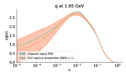
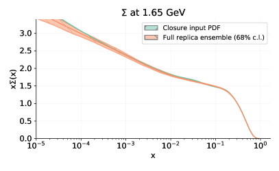
Figure 6.1: The replica (solid green line) chosen as the true underlying PDF $\boldsymbol{f}$ for the closure test: the gluon (left) and quark singlet (right) are displayed. The NNPDF4.0 central value and 68% confidence interval (same as in Fig. 5.2) are also shown for reference.

We have performed a closure test by assuming as input PDF set used to produce the true observable values $\boldsymbol{f}$ a specific replica randomly selected out of the $N_{\rm rep}$ replicas of the NNPDF4.0 NNLO global determination. The reason for this choice is that on the one hand, it automatically satisfies known theoretical constraints, such as the sum rules of Sect. 3.1.2. On the other hand, thanks to it being randomly selected out of a replica sample, it satisfies the criteria of flexibility and model-independence of Sect. 6.1.2. In particular, individual replicas have generally more structure than the final central PDF, so by choosing a repica, rather than the central fit from either NNPDF or any other PDF set, we are making the closure test somewhat more stringent. The specific replica that we chose is shown in Fig. 6.1 (gluon and quark singlet), together with the NNPDF3.1 central value and uncertainty.

We have produced $n_{\rm fit}=25$ sets of data Eq. (6.1), each of which has been used to produce a fit with $N_{\rm rep}=40$ replicas. Results are then bootstrapped [223, 224] in order to improve stability. We have checked that increasing the number of replicas or the number of fits results are unchanged within the bootstrap uncertainty. The fits are produced using the NNPDF3.1-like dataset discussed in Sect. 2.1.

Data space estimators, such as the bias-to-variance ratio $\mathcal{R}_{bv}$, are produced by selecting out of the full datasets that enter the NNPDF4.0 determination all data that were not already used for fitting. An advantage of this choice is that the kinematic coverage of the fitting dataset and the testing dataset are then reasonably similar, thus ensuring Gaussianity, as discussed above,

In PDF space, we perform tests for PDFs in the evolution basis at the PDF parametrization scale and over a grid of $x$ points, chosen for the gluon and singlet as logarithmically spaced for $10^{-3}<x<0.1$ and linearly spaced for $0.1<x<0.5$, and for nonsinglet quark distributions $V$, $V_{3}$, $T_{3}$, and $T_{8}$ as purely linearly spaced for $0.1<x<0.5$. We do not consider the $V_{8}$ and $T_{15}$ nonsinglet combinations that are too noisy at the initial scale. Furthermore, we evaluate $\xi_{1\sigma}$ in Eq. (6.16) with $n_{x}=4$ to reduce the correlations between points, and we also rotate into the basis which diagonalizes the covariance estimated on the PDF replicas as an extra precaution.

6.1.4 Validation of the NNPDF4.0 methodology

We now turn to the validation of the NNPDF4.0 methodology. First of all, we evaluate the expectation value of $\Delta_{\chi^{2}}$, Eq. (6.9), over the $n_{\rm fit}$ fits that constitute the NNPDF4.0 closure tests and present in Table 6.1 the results separated into groups of datasets. As mentioned, the input dataset is NNPDF3.1-like. One can observe how $\mathbf{E}_{\eta}\left[\Delta_{\chi^{2}}\right]<0$ for all datasets considered, indicating the absence of under-fitting. Furthermore, its small absolute magnitude, typically at the per-mille level or at most being a couple of percent, corresponds to a negligible amount of overfitting, and it is thus consistent with proper learning.

	$N_{\rm dat}$	$\mathbf{E}_{\eta}\left[\Delta_{\chi^{2}}\right]$
Dataset
DIS NC	2100	-0.0059
DIS CC	989	-0.0112
DY	712	-0.0148
Top	19	-0.0054
Jets	273	0.0001
Total	4093	-0.0087

Table 6.1: The expectation value of $\Delta_{\chi^{2}}$, Eq. (6.9), evaluated over the $n_{\rm fit}$ fits that constitute the NNPDF4.0 closure test. Results are presented separated into different processes.

We now turn to the bias-to-variance ratio $\mathcal{R}_{bv}$, Eq. (6.15), which is shown in Table 6.2, evaluated for testing datasets that were not used as input to the closure test fits, with results divided by groups of processes. The combination of the fitting set used to evaluate Table 6.1 and the testing set shown here add up to the complete NNPDF4.0 baseline dataset. The last column indicates the uncertainty of the $\mathcal{R}_{bv}$, determined as its standard deviation over a bootstrap sample of both fits and replicas.

For the total testing set, it is found that $\mathcal{R}_{bv}\simeq 1$ within the bootstrap error, demonstrating the faithfulness of the estimated PDF uncertainties.

	$\mathcal{R}_{bv}$	bootstrap error
Dataset
DY	0.99	0.08
Top pair	0.75	0.06
Jets	1.14	0.05
Dijets	0.99	0.07
Direct photon	0.71	0.06
Single top	0.87	0.07
Total	1.03	0.05

Table 6.2: The bias-to-variance ratio $\mathcal{R}_{bv}$, Eq. (6.15), divided by groups of processes and evaluated for the testing datasets that were not used as input to the NNPDF4.0 closure test fits. The last column indicates the uncertainty associated to $\mathcal{R}_{bv}$, determined as its standard deviation over a bootstrap sample of both fits and replicas.

In order to gain some more understanding of the results from Table 6.2, it is instructive to plot the full distributions of both the total bias, Eq. (6.7), and of the total variance, Eq. (6.8), over the $n_{\rm fits}$ constituting the NNPDF4.0 closure tests. From these two distributions, displayed in Fig. 6.2, one can observe that not only are their means consistent, but also that they exhibit a similar shape. The only difference is that the distribution over the variances is somewhat broader, with a small tail towards large values of the estimator. Since each of the $n_{\rm fit}$ fits has 40 replicas, one expects better statistics in the distributions over variances as compared to that over biases, which is why the tail of the former is better sampled. Furthermore, we performed checks that the results in Table 6.2 are stable upon removing selected fits and replica within the bootstrap uncertainty, and hence we are confident that the results are not subject to finite size effects.

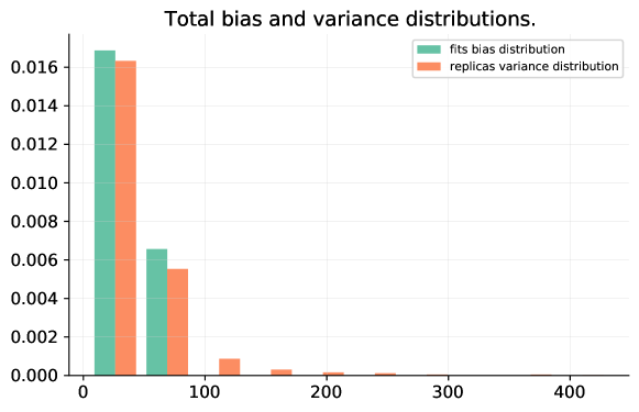
Figure 6.2: The normalized distribution of the total bias, Eq. (6.7), and of total variance, Eq. (6.8), over the $n_{\rm fits}$ constituting the NNPDF4.0 closure tests. The square root of the mean of these two distributions defines $\mathcal{R}_{bv}$, the bias-to-variance ratio.

The fact that the bias-to-variance ratio satisfies $\mathcal{R}_{bv}\simeq 1$ both for the total testing dataset and at the level of groups of processes indicates that the PDF uncertainties in the NNPDF4.0 methodology are being faithfully estimated. Further confirmation of this property can be obtained by evaluating the quantile estimators in both PDF and data space, respectively defined in Eqs. (6.16, 6.17). First of all, Table 6.3 displays the one-sigma quantile estimator in the space of experimental data, $\xi^{(\rm data)}_{1\sigma}$, evaluated for the same testing dataset as that used for Table 6.2, together with the corresponding bootstrap error. In addition, we also indicate the value of ${\rm erf}(\mathcal{R}_{bv}/\sqrt{2})$ evaluated using the corresponding bias-to-variance ratio. As indicated by Eq. (6.18), for a successful closure test one expects that these two quantities coincide, that is, $\xi^{(\rm data)}_{1\sigma}\simeq{\rm erf}(\mathcal{R}_{bv}/\sqrt{2})$.

It is clear that $\xi^{(\rm data)}_{1\sigma}$ and ${\rm erf}(\mathcal{R}_{bv}/\sqrt{2})$ agree well with each other within the bootstrap error, which provides a non-trivial consistency test. Furthermore, $\xi^{(\rm data)}_{1\sigma}=0.68$ for the total dataset as expected, with reasonable fluctuations between different process types. The observed deviations between the two indicators may be explained by quantile statistics being more robust to outliers, or because the value of ${\rm erf}(\mathcal{R}_{bv}/\sqrt{2})$ can be dominated by a few eigenvectors of the experimental covariance matrix.

	$\xi^{(\rm data)}_{1\sigma}$	bootstrap error	${\rm erf}(\mathcal{R}_{bv}/\sqrt{2})$	bootstrap error
experiment
DY	0.69	0.02	0.69	0.04
Top	0.75	0.03	0.82	0.03
Jets	0.63	0.03	0.62	0.02
Dijets	0.70	0.03	0.69	0.04
Direct photon	0.81	0.03	0.84	0.03
Single top	0.69	0.04	0.75	0.04
Total	0.68	0.02	0.67	0.03

Table 6.3: The one-sigma quantile estimator in the space of experimental data, $\xi^{(\rm data)}_{1\sigma}$ iEq. (6.17) and evaluated for the same testing dataset as used for Table 6.2, together with the corresponding bootstrap error. For each group of processes, we also display the value of ${\rm erf}(\mathcal{R}_{bv}/\sqrt{2})$ evaluated using the corresponding bias-to-variance ratio.

In order to provide a graphical representation of the information contained in Table 6.3, it is instructive to evaluate the difference between the mean value (over replicas) of the theory predictions and the corresponding truth observable values normalized by the PDF uncertainties, that is

$$\delta_{i}^{(l)}\equiv{{\left(\mathbf{E}_{\epsilon}\left[g_{i}\right]^{(l)}-f_{i}\right)}\over{\sigma_{i}^{(l)}}}\,,\qquad i=1,\ldots,N_{\rm dat}\,,\qquad l=1,\ldots,n_{\rm fit}\,.$$ (6.19)

The normalized distribution of these relative differences $\delta_{i}^{(l)}$ is displayed in the left panel of Fig. 6.3 together with a univariate zero-mean Gaussian for reference. The fraction of the histogram entries which fall inside the 1-sigma confidence interval of the scaled Gaussian is then equal to the value of the total $\xi^{(\rm data)}_{1\sigma}$ displayed in Table 6.3.

From Fig. 6.3 it is apparent that the central values of the model predictions for physical observables fluctuate around the true values by an amount which is consistent with the expectations of the associated PDF uncertainties. Indeed, there is excellent agreement between the distribution of $\delta_{i}^{(l)}$ and that of the reference Gaussian, consistently with the value of $\xi^{(\rm data)}_{1\sigma}=0.68$ reported in Table 6.3.

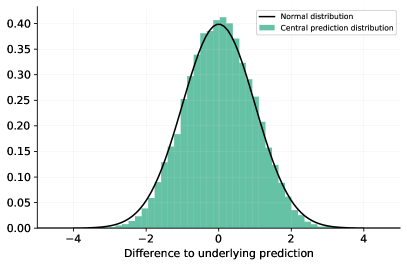
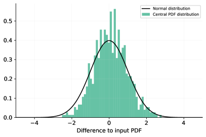
Figure 6.3: The normalized distribution of relative differences $\delta_{i}^{(l)}$ in data data space Eq. (6.19 (left) or $\widetilde{\delta}_{i,j}^{(l)}$ Eq. (6.20 in PDF space (right). In both cases, a univariate zero-mean Gaussian distribution is plotted for reference.

We now compute the quantile estimator in PDF space, defined in Eq. (6.16). This estimator, $\xi_{n\sigma}^{\rm(pdf)}$, was already introduced as part of the original study in [14]. However, as mentioned it was only possible to evaluate it approximately, as performing multiple closure test fits was computationally infeasible. The values of $\xi_{1\sigma}^{\rm(pdf)}$ are presented in Table 6.4, along with their bootstrap error. In general, there is reasonable agreement within bootstrap errors between the computed value of $\xi_{1\sigma}^{(\rm pdf)}$ and the expected value of 0.68. However, in comparison to the corresponding estimator in data space larger fluctuations are observed, specifically for the singlet PDF $\Sigma$, and the average value $\xi_{1\sigma}^{(\rm pdf)}=0.71\pm 0.02$ is somewhat overestimated. It should be noticed that the PDF-space estimator is somewhat less stable and accurate than that in data space, due to the need to pick a grid of points that corresponds to the measured region, and also because of the very high correlation between PDFs at neighboring points which may lead to an unstable covariance matrix. The fact that the average $\xi_{1\sigma}^{(\rm pdf)}$ is slightly more than 0.68 suggests that anyway PDF uncertainties are conservatively estimated.

	$\xi^{\rm(pdf)}_{1\sigma}$	bootstrap error
flavor
$\Sigma$	0.82	0.04
$g$	0.70	0.05
$V$	0.65	0.05
$V_{3}$	0.63	0.05
$V_{8}$	0.72	0.04
$T_{3}$	0.71	0.05
$T_{8}$	0.71	0.05
Total	0.71	0.02

Table 6.4: The values of the quantile estimator in PDF space, $\xi_{1\sigma}^{\rm(pdf)}$ Eq. (6.16), separated into the contributions from individual flavor combinations together with the corresponding bootstrap uncertainty.

Finally, in Fig. 6.3 the histogram of relative differences is also shown using a PDF space definition:

$$\widetilde{\delta}_{i,j}^{(l)}\equiv{{\left(\mathbf{E}_{\epsilon}\left[q^{i(l)}(x_{j})\right]-q_{\rm in}^{i}(x_{j})\right)}\over{\sigma^{i(l)}(x_{j})}}\,,\quad i=1,\ldots,n_{\rm flav}\,,\quad j=1,\ldots,n_{x}\,,\quad l=1,\ldots,n_{\rm fit}\,,$$ (6.20)

We see that, even though also in this case there is excellent agreement with the expected univariate Gaussian behavior, results are indeed rather noisier than in data space.

6.1.5 Extent and limitations of closure testing.

The closure tests presented in this section are entirely successful, thereby validating the NNPDF4.0 methodology in the data region. However, it is important to understand what the closure tests do and do not verify.

The closure test, at least in its present incarnation, makes two assumptions. The first is that the underlying distribution of the experimental data is known exactly. Specifically, if the data are Gaussian, it is assumed that their distribution is unbiased and that the covariance that characterizes this multi-Gaussian distribution is fully known. In realistic situations, of course, this, even in the best of hypotheses, can only be approximately the case, since the experimental covariance matrix is itself an observable which is extracted from the data, and thus it is characterized by an uncertainty on the uncertainty. Furthermore, some sources of systematic uncertainty are based on theoretical estimates and thus subject to theoretical uncertainties which are difficult to estimate. Finally, in the worst case it may happen that some data or the associated uncertainty are simply incorrect: this would correspond to a biased distribution (wrong central value) or an incorrect uncertainty or correlations (wrong covariance matrix).

The second assumption is that the data are obtained from the PDF using a known underlying physical law. In realistic situations this is surely not the case, since theoretical predictions are computed at finite perturbative accuracy, and thus data predictions are affected by an uncertainty corresponding to the very least to missing higher order perturbative corrections, and generally also to other possible corrections such as nuclear effects, electroweak corrections, heavy quark mass effects, limited knowledge of standard model parameters, and so on.

Therefore, the closure test presented here checks for faithfulness of the component of the PDF uncertainty which is induced by the data uncertainty, assuming the latter is perfectly known. It does not check for other sources of uncertainty, such as theory uncertainties: this would have to be added separately. A methodology for doing so was discussed and applied to missing higher order perturbative uncertainties in Refs. [23, 24], but is not implemented in a global NNLO PDF determination yet. Also, it does not account for possible “data inconsistencies”, i.e., incorrectly estimated experimental values and uncertainties. This motivates the need to select a maximally consistent dataset, as we have done in Sect. 4, that guarantees that no major inconsistencies are present in the baseline dataset. However, remaining small inconsistencies might still lead to a certain amount of uncertainty underestimation, whose exact assessment will require performing closure tests with artificial inconsistent data.

6.2 Future testing NNPDF4.0

The closure tests presented in Sect. 6.1 allow for an assessment of the faithfulness of PDF uncertainties in the region covered by available experimental data. However, they are ill-suited for an assessment of the behavior of PDFs and their uncertainties in the extrapolation regions where little or no experimental constraints are available, for a variety of reasons, the most obvious of which is that the multi-Gaussian assumption is likely to fail outside the data region

Hence, closure tests have limited applicability to study the generalization power of the resulting PDF fit to new, unexplored kinematic regions. A more suitable strategy to assess this generalization power are the so-called “future tests” proposed in [15]. The main idea underlying future tests is that what we ask for in an extrapolation region is that PDF uncertainties correctly reflect the lack of information. Whereas in principle in the absence of information uncertainties are infinite, in practice PDF uncertainties not too far from the data region are constrained by requirements of continuity and smoothness. Whereas in the absence of direct information we cannot expect to be able to achieve a full and detailed knowledge of the covariance between any two PDFs (or indeed any two predicted data points), we do wish for PDF uncertainties to reproduce the possible deviation of the best-fit PDFs, and of physical predictions obtained using them, from the true value that would be obtained if the PDF was known say as accurately as it is known in the data region.

The future test verifies explicitly whether this is the case: a “future test PDF” is determined from a restricted subset of the full dataset that only covers a limited region. This future test PDF is then used to predict all the rest of the dataset. The restricted datasets can be thought of as representative of the limited knowledge that was available at some point in the past, (hence the name “future test”) but this is of course just a manner of speaking, as any partitioning of the dataset into restricted and full may be considered. Because future tests of NNPDF3.1 were never performed, here we will present future tests of both the NNPDF3.1 and NNPDF4.0 methodologies. This allows us to simultaneously validate the new methodology, and also put it in context.

6.2.1 Future testing methodology

Following the discussion in [15] we test the NNPDF3.1 and NNPDF4.0 methodologies by choosing as input specific subsets of the complete NNPDF4.0 baseline dataset, and determining corresponding PDF sets from them. The predictions obtained using these PDFs are then compared to the data not included in their fit, in order to assess whether the uncertainty in the prediction correctly accounts for the correspondingly missing information.

This is done by evaluating the $\chi^{2}$ to the datasets not used in the fit with PDF uncertainties also included along with the data uncertainties in the $\chi^{2}$ definition. Indeed, we expect in general that the $\chi^{2}$ evaluated including data uncertainties only should be larger than one, as soon as the deviation of the PDF from its true value is larger than the experimental uncertainty, which is bound to happen for sufficiently accurate data in an extrapolation region. However, if the deviation from the true value is correctly reproduced by the PDF uncertainty, the $\chi^{2}$ should then become again close to one once the PDF uncertainty is included. Note that the test is only nontrivial if the $\chi^{2}$ value before inclusion of the PDF uncertainty is significantly larger than one: otherwise, the data are not precise enough to test for faithfulness of the PDF uncertainty.

Specifically the $\chi^{2}$ with PDF uncertainties included is computed using the covariance matrix

$${\rm cov}_{ij}^{\rm(tot)}={\rm cov}_{ij}^{\rm(exp)}+{\rm cov}_{ij}^{\rm(pdf)}\,,$$ (6.21)

where ${\rm cov}_{ij}^{\rm(exp)}$ is the usual experimental covariance matrix, while the covariance matrix ${\rm cov}_{ij}^{\rm(pdf)}$ corresponding to PDF uncertainties can be determined as

$${\rm cov}_{ij}^{\rm(pdf)}=\left\langle\mathcal{F}_{i}\mathcal{F}_{j}\right\rangle_{\rm rep}-\left\langle\mathcal{F}_{i}\right\rangle_{\rm rep}\left\langle\mathcal{F}_{j}\right\rangle_{\rm rep}\,,$$ (6.22)

where $\mathcal{F}_{i}^{(k)}$ is the $i$-th physical prediction found using the $k$-th replica of a given PDF set, and the average is performed over replicas. Simply combining the two covariance matrices according to Eq. (6.21) is justified when the corresponding sources of uncertainty are uncorrelated [24]. This is clearly the case since the experimental uncertainty on data which are not fitted is completely independent of the PDF uncertainty, as the latter is driven by the uncertainty on the fitted data.

6.2.2 Future testing datasets

We choose three subsets of the full NNPDF4.0 datasets, inspired by the chronological order in which actual measurements became available, respectively chosen to correspond approximately to a “pre-HERA” and “pre-LHC” dataset, and to the NNPDF3.1-like dataset that was used as fitting dataset in the closure tests of Sect. 6.

They are defined as follows:

• Pre-HERA. Only fixed-target DIS structure function data and fixed-target Drell-Yan cross-sections data are included.

• Pre-LHC. This is a superset of the pre-HERA dataset, which is extended to also include HERA collider inclusive and charm structure function data, and Tevatron $W$ and $Z$ production data.

• NNPDF3.1-like. This is the dataset defined in Ref. [10] and used as fitting dataset in the closure tests presented in Sect. 6.

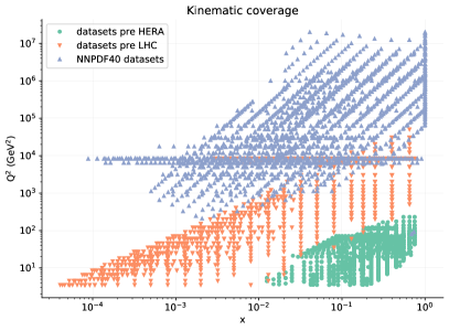
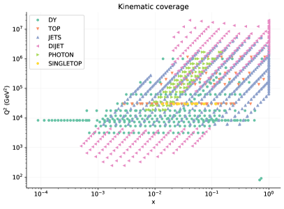
Figure 6.4: Scatter plots comparing various future test data subsets to the full NNPDF4.0 of Fig. 2.1. Left: comparison of the pre-HERA, pre-LHC and NNPDF4.0 datasets. Note that each dataset is a superset of the previous one, so all the pre-HERA data are included in the pre-LHC set, and all data are included in the NNPDF4.0 set. Right: the data points which are included in NNPDF4.0 but not in the NNPDF3.1-like dataset, grouped by process type.

It is important to draw a distinction between the NNPDF3.1-like dataset and the other two subsets; while going from pre-HERA to pre-LHC to NNPDF4.0 consecutively adds data in new kinematic regions, going from NNPDF3.1-like to NNPDF4.0 instead adds more data points in regions for which data already exist. So we can think of the transition from NNPDF3.1 to NNPDF4.0 as an interpolation rather than an extrapolation. This is reflected in scatter plots in Fig. 6.4, where the difference between the first two subsets and NNPDF4.0 are shown on the left, and the difference between the NNPDF3.1-like subset and NNPDF4.0 is shown on the right.

More specifically, first (left) we compare the pre-HERA, pre-LHC and full NNPDF4.0 datasets. Note that the pre-LHC dataset contains the points marked with an orange triangle as well as the pre-HERA points, and the NNPDF4.0 dataset contains all points: the three datasets are each a superset of the previous one. It is also clear that each dataset probes an increasingly wide kinematic region. Specifically, pre-HERA data are restricted to $x\mathrel{\hbox to0.0pt{\lower 4.0pt\hbox{\hskip 1.0pt$\sim$}\hss}\raise 1.0pt\hbox{$>$}}0.01$ and $Q^{2}\mathrel{\hbox to0.0pt{\lower 4.0pt\hbox{\hskip 1.0pt$\sim$}\hss}\raise 1.0pt\hbox{$<$}}200$ GeV, while pre-LHC data cover the complete range of $x$ but only $Q^{2}\mathrel{\hbox to0.0pt{\lower 4.0pt\hbox{\hskip 1.0pt$\sim$}\hss}\raise 1.0pt\hbox{$<$}}10^{5}$ GeV. Furthermore, each dataset provides an increasingly wide handle on specific PDFs or PDF combinations: for instance, pre-HERA data provide little handle on quark flavor decomposition, and pre-LHC data provide essentially no handle on the large-$x$ gluon. The pre-HERA and pre-LHC allow us to test for far-extrapolation (pre-HERA) and near-extrapolation (pre-LHC).

Then (right) we show all the data that are included in NNPDF4.0 but not in the NNPDF3.1-like dataset, classified by process type. In this case the kinematic region covered by the new datasets included in NNPDF4.0 essentially overlaps with the NNPDF3.1-like dataset, though with a lower density. Hence, in this case it is interpolation, rather than extrapolation, what is being tested.

6.2.3 Future test results

We now present results of future testing both the NNPDF4.0 and NNPDF3.1 methodologies. We first discuss the case of near and far extrapolation, namely, the pre-HERA and pre-LHC datasets. The $\chi^{2}$ values for all data, divided by process type, are collected in Table 6.5. For either methodology we have determined three PDF sets from the three datasets, and we show $\chi^{2}$ values obtained using each of them. The process-type classification is made in such a way that the data for any given process type are either all included, or all excluded in the determination of each of the three PDF sets. When a process type is not included in the PDF determination both the $\chi^{2}$ value without PDF uncertainty (in italic) and the PDF value with PDF uncertainty (in boldface) are shown. All other $\chi^{2}$ values correspond to fitted data. We also tabulate $\chi^{2}$ values for the full set of data which in each case is not fitted, denoted as out-of-sample data.

	$N_{\rm dat}$	NNPDF3.1 methodology			NNPDF4.0 methodology
Process		pre-HERA	pre-LHC	Global	pre-HERA	pre-LHC	Global
Fixed target NC DIS	973	1.07	1.21	1.27	1.05	1.18	1.23
Fixed target CC DIS	908	0.97	1.06	1.14	0.80	0.85	0.87
Fixed target Drell-Yan	89	0.87	1.03	1.28	0.92	1.27	1.59
HERA	1208	35.75 (1.18)	1.21	1.20	27.20 (1.23)	1.22	1.20
Collider Drell-Yan (Tevatron)	65	16.95 (0.98)	0.93	1.00	5.52 (1.02)	0.99	1.11
Collider Drell-Yan (LHC)	116	22.96 (1.03)	3.39 (1.31)	1.61	18.91 (1.31)	2.63 (1.58)	1.53
Top quark production	83	9.63 (0.63)	1.31 (0.65)	0.90	20.01 (1.06)	1.30 (0.87)	1.01
Jet production	500	4.92 (0.88)	3.13 (0.99)	1.43	2.69 (0.98)	2.12 (1.10)	1.26
Total out-of-sample		25.46 (1.07)	2.96 (1.00 )	$-$	19.48 (1.16)	2.10 (1.15)	$-$
Total	3942	13.20	1.47	1.24	10.21	1.28	1.15

Table 6.5: Values of the $\chi^{2}$ per datapoint for the total dataset and for specific process types obtained for NNPDF4.0 and for the pre-HERA and pre-LHC future test PDFs, determined using NNPDF3.1 or NNPDF4.0 methodology. All the data in each process type are either fully included or fully excluded from each PDF determination. Values in regular font correspond to fitted datasets, evaluated with the experimental covariance matrix. Values in bold or italics correspond to data that are not fitted. The value in italic is evaluated with the experimental covariance matrix, while the value in bold also includes PDF uncertainties, Eqs. (6.21-6.22). Values of $\chi^{2}$ for the full set of data that are not fitted (denoted as total out-of-sample) is also given in each case.

First, we note that the total $\chi^{2}$ for out-of-sample data is very large (of order twenty) for pre-HERA PDFs while it is moderately large (of order three) for pre-LHC PDFs. This shows that the test is nontrivial in both cases, and it indeed tests for far-extrapolation for pre-HERA and near-extrapolation for pre-LHC. A similar pattern is observed for all process types: HERA, that probes the small $x$ gluon, top and jets, that probe the large $x$ gluon, and Drell-Yan, that probes quark flavor separation.

When the PDF uncertainties are introduced, all $\chi^{2}$ values become of order one, thereby showing that the future test is successful. This is especially remarkable given that in some cases (such as HERA data or collider Drell-Yan data for the pre-HERA PDFs) the reduction in $\chi^{2}$ is by almost a factor 30. This means that the PDF uncertainty accounts for a deviation between data and theory which is over five times bigger than the data uncertainty.

Finally, comparing the two methodologies it is clear that both are equally successful in satisfying the future tests. However, with NNPDF3.1 methodology $\chi^{2}$ values computed without PDF uncertainty for out-of-sample data are rather larger than with NNPDF4.0 methodology. This means that while both methodologies lead to faithful uncertainties in the extrapolation region, NNPDF4.0 has smaller extrapolation uncertainties, i.e., it provides a more efficient generalization of the fitted data.

We then turn to fits based on the NNPDF3.1-like dataset. In this case, each process type is represented both in the fitted and extrapolation dataset, hence in Table 6.6 we only show $\chi^{2}$ values for the total fitted and out-of-sample datasets. In this case, the out-of-sample $\chi^{2}$ is smaller than two, and smaller than 1.5 for NNPDF4.0 methodology consistent with the fact that the out-of-sample data are now in an interpolation region. Also in this case, upon inclusion of the PDF uncertainty all $\chi^{2}$ value become of order one, and close to the $\chi^{2}$ value for the fitted dataset.

	NNPDF3.1 methodology		NNPDF4.0 methodology
	NNPDF3.1-like	Global	NNPDF3.1-like	Global
$\chi^{2}_{\rm exp}$	1.74	1.29	1.46	1.20
$\chi^{2}_{\rm exp+pdf}$	1.12	$-$	1.17	$-$

Table 6.6: Same as Table 6.5, now for the NNPDF3.1-like future test.

We conclude from this analysis that the future test is fully successful for both methodologies, and that for the same datasets near- and far-extrapolation and interpolation uncertainties are smaller with NNPDF4.0 methodology as compared to its NNPDF3.1 counterpart.

By construction, the performance of future tests should always be assessed at the level of $\chi^{2}$. However, for the sake of visualization, we also provide some comparisons, both at the PDF level and at the data level, between future-test PDFs and PDFs determined from the global NNPDF4.0 baseline dataset. In Fig. 6.5 and Fig. 6.6 we compare future test pre-HERA and pre-LHC PDFs at the parametrization scale to those determined using the full dataset, using respectively the NNPDF3.1 and NNPDF4.0 fitting methodologies. The inflation of PDF uncertainties when a particular $x$ range for a given PDF changes from data to extrapolation between different sets is apparent. The smaller extrapolation uncertainty found using NNPDF4.0 methodology in comparison to the NNPDF3.1 methodology is also visible. Finally, it is clear that there is good overall compatibility of all PDFs when comparing the data region of one set to the extrapolation region of a different set, in agreement with the $\chi^{2}$ values of Table 6.5. A possible exception is the gluon from the pre-HERA future test which, while compatible with the global result when using NNPDF3.1 methodology, disagrees with it at the two sigma level or even more when using NNPDF4.0 methodology in the $x\lesssim 0.002$ region. This might be due to the poor internal consistency of the BCDMS and NMC data already noted in Sect. 4.2.4: if so, this would indicate that the NNPDF4.0 methodology is sensitive enough to pick up this, while the NNPDF3.1 methodology is not.

Finally, in Fig. 6.7 we compare predictions obtained using the pre-HERA, pre-LHC, and global (NNPDF4.0) PDFs to a representative selection of data included in the global fit but not in the pre-LHC fit. Specifically, we consider the HERA NC structure functions at $\sqrt{s}=920$ GeV in the $Q=1.871$ GeV bin; the dimuon rapidity distributions in forward $Z\to\mu\mu$ production at LHCb; the top quark rapidity distributions in the ATLAS $t\bar{t}$ lepton+jet measurement at 8 TeV; and the dilepton rapidity distribution for $M_{\ell\ell}=25$ GeV and the CMS double-differential Drell-Yan measurement at 7 TeV. Of these, only the HERA structure function data are included in the pre-LHC fit, though of course not in the pre-HERA fit, while all other data are predictions for both future-test PDF sets. All results displayed in these comparisons have been obtained using NNPDF4.0 methodology. A historical curiosity here is the observation that the rise of the $F_{2}$ structure function at HERA, which came as a surprize (see e.g. Refs. [225, 226]) is correctly reproduced by the pre-HERA fit based on its onset in pre-HERA data. Note however that this should not be taken as a prediction: both methodologies that we are testing here have been developed based on later datasets, and thus do encode to some extent some of the information contained in the later data.

The very large difference between fitted and extrapolation PDF uncertainty is apparent, and so is the hierarchy between near-extrapolation uncertainties (pre-LHC) and far-extrapolation uncertainties (pre-LHC), e.g. for the top pair production data. The good compatibility between data and predictions including PDF uncertainties is also clear, again confirming the success of the future test as summarised in Table 6.5.

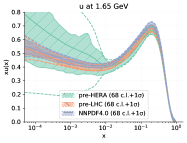
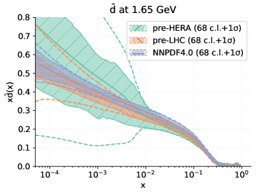
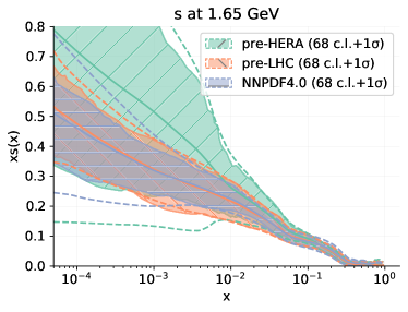
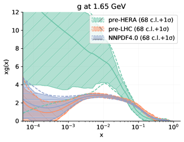
Figure 6.5: Some pre-HERA and pre-LHC PDFs compared to PDFs based on full NNPDF4.0 dataset, in all cases obtained using the NNPDF3.1 fitting methodology. The up (top left), antidown (top right), strange (bottom left) and gluon (bottom right) are shown at the input parametrization scale of $Q=1.65$ GeV.

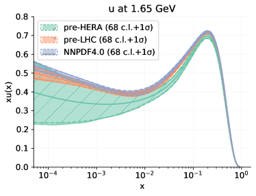
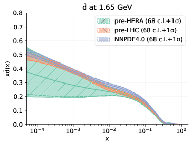
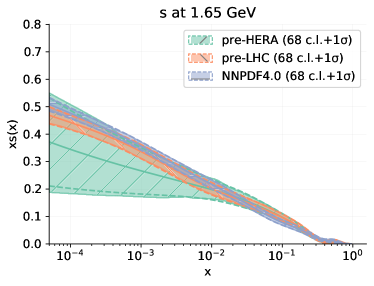
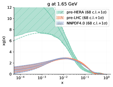
Figure 6.6: Same as Fig. 6.5, but now showing PDFs determined using the NNPDF4.0 methodology.

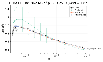
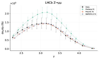
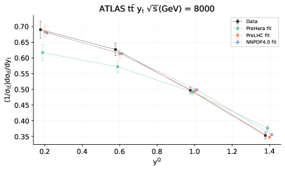
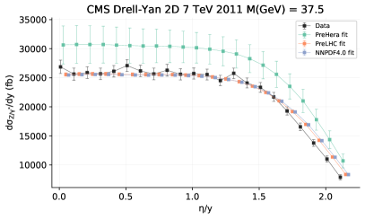
Figure 6.7: Comparison of the theoretical predictions including PDF uncertainties from the pre-HERA and pre-LHC PDF sets based on NNPDF4.0 methodology and those of the global fit to four representative measurements: t HERA NC structure functions, dimuon rapidity distributions in $Z$ production at LHCb, top rapidity distributions in ATLAS $t\bar{t}$ production, and the dilepton rapidity distribution for CMS double-differential Drell-Yan (see text for details). Note that only the HERA structure function data enter the pre-LHC fit (but not the pre-LHC fit), and all the remaining data do not enter either the pre-HERA or pre-LHC fit. The uncertainty in the data corresponds to the total diagonal experimental error.

7 Dataset dependence of the NNPDF4.0 parton set

Having established the reliability of the NNPDF4.0 determination, we now study in detail the impact on the PDFs of the data (in this section) and of the methodology (in the next section). This also provides us with further a posteriori checks of the stability and reliability of our results.

In this Section, we first assess the global impact of the change in dataset when going from NNPDF3.1 to NNPDF4.0, and then we present variants of the baseline NNPDF4.0 fit, in which the impact of specific datasets is studied by removing them from the baseline. Finally, we assess the impact of datasets that have not been included in the NNPDF4.0 baseline, with the main aim of checking the stability of our results. Whereas the analysis presented in this section gives some indication on the pull of some data on individual PDFs, a full assessment of the impact of various data on the PDFs would require the use of correlation tools such as presented in Ref. [27], as well as systematic studies of PDFs based on partial datasets, such as presented in Sect. 2.3 of Ref. [227] in the context of the NNPDF2.3 determination.

Except otherwise stated, all the fits presented in this section utilize the methodology discussed in Sect. 3 and correspond to Monte Carlo ensembles of 100 replicas.

7.1 Impact of the updated dataset

As explained in Sect. 2.1, the NNPDF4.0 dataset differs from NNPDF3.1 not only because of the addition of a significant amount of measurements not included in NNPDF3.1, but also because of changes in the treatment of some of the data already included in NNPDF3.1, mostly related to updates in the data and in the corresponding theory calculations. These changes are incorporated in a dataset called NNPDF3.1-like in Sect. 2.1 and used throughout this paper whenever comparisons to NNPDF3.1 are required, e.g. in the code benchmarks of Sect. 3.4 or in the future tests of Sect. 6.2. However, in Sect. 5.2.1 (specifically in Fig. 5.2) we compared NNPDF4.0 to the published NNPDF3.1 set. We must therefore start this discussion of dataset dependence with an assessment of the differences between the published NNPDF3.1 fit and its update based on this NNPDF3.1-like dataset.

7.1.1 The NNPDF3.1-like dataset and PDFs

The impact of the alterations made to the NNPDF3.1 dataset are studied by comparing the original NNPDF3.1 determination [5] to a PDF fit based on same NNPDF3.1 methodology but using the NNPDF3.1-like dataset discussed in Sect. 2.1. The corresponding PDFs are compared in Fig. 7.1.

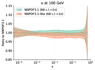
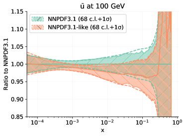
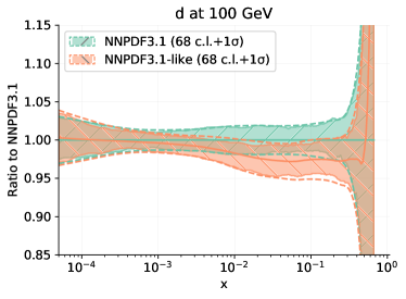
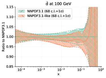
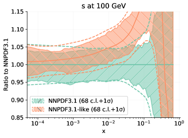
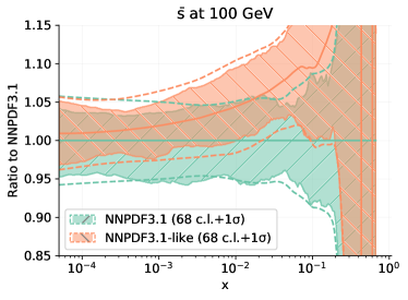
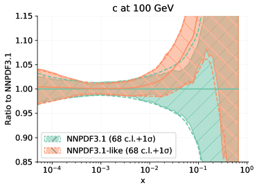
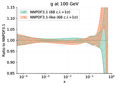
Figure 7.1: The up, antiup, down, antidown, strange, antistrange, charm and gluon PDFs from NNPDF3.1 and from a fit based on the same NNPDF3.1 methodology but on the NNPDF3.1-like dataset defined in Sect. 2.1. Results are displayed at $Q=100$ GeV, normalized to the NNPDF3.1 central value. Solid and dashed bands correspond to 68% and one-sigma uncertainties, respectively.

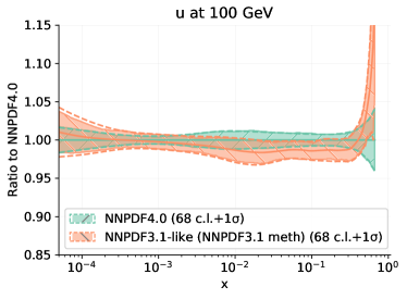
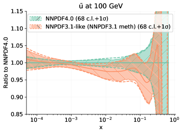
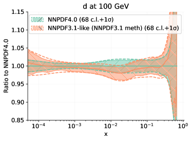
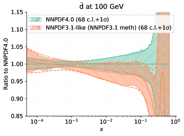
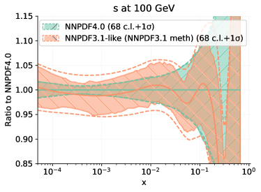
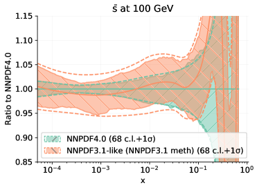
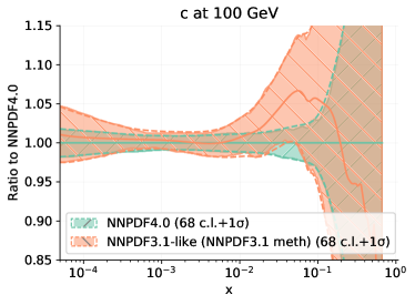
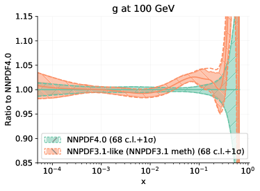
Figure 7.2: Same as Fig. 5.2 but now comparing NNPDF4.0 to NNPDF3.1-like instead of the published NNPDF3.1. The NNPDF3.1-like PDFs shown here define the NNPDF3.1 baseline which will be used in all subsequent plots in this section.

As expected, the two PDF sets are overall well consistent, with the PDF central values of each set being almost always included in the PDF uncertainties of the other across the entire range of $x$. Some differences are nevertheless seen for individual PDFs. These are the largest for the strange quark and antiquark PDFs. In this case, differences are mostly explained by the improved treatment of the NuTeV data: the NNPDF3.1-like dataset incorporates NNLO massive QCD corrections to the dimuon cross-sections [139], which were not available at the time the original NNPDF3.1 set was produced, and an update of the value for the branching ratio of charmed hadrons into muons (see Sect. 2.1 and the discussion of [10].)

The combined effect of these two updates is an enhancement of the strange quark and antiquark PDFs in comparison to the original NNPDF3.1 analysis, already reported in Ref. [10]. To compensate for this effect, the down quark and antiquark PDFs are correspondingly suppressed. In the case of the charm PDF, a different behavior of the central value is observed for $x\gtrsim 0.01$, possibly because of the replacement of the HERA charm cross-section data with their final combined version, see Sect. 2. Finally, slight differences in the gluon PDF are likely due the different treatment of single-inclusive jet data: Tevatron and 2.76 TeV ATLAS and CMS measurements are no longer included in the NNPDF3.1-like dataset, and NNLO $K$-factors, computed with the recommended choice of scale, are incorporated for the remaining 7 TeV ATLAS and CMS measurements (no NNLO $K$-factors were used in NNPDF3.1, as they were not yet available). The precision of the PDFs in the two parton sets is almost identical. We conclude that the difference in strange PDFs between the published NNPDF3.1 and NNPDF4.0 observed in Sect. 5.2.1 is due to these reasons.

We conclude that the NNPDF3.1-like dataset is compatible with NNPDF3.1 but not identical to it, with differences due to updates in either the data, or their theoretical treatment after the original NNPDF3.1 PDF set was produced. Henceforth, in this and the next section, we will always compare to this updated NNPDF3.1-like PDF set and dataset, and by “NNPDF3.1 baseline” will always refer to the PDFs obtained with NNPDF3.1 methodology and NNPDF3.1-like dataset. For completeness, these NNPDF3.1 baseline PDFs are also shown in Fig. 7.2, compared now to the NNPDF4.0 baseline. Of course, the overall pattern is very similar to that of the comparison between NNPDF4.0 and the published NNPDF3.1 previously shown in Fig. 5.2. Fig. 7.2 will serve as a reference when assessing the relative impact of data and methodology in driving the differences between NNPDF3.1 and NNPDF4.0.

7.1.2 Impact of the new data in NNPDF4.0

The impact of the new measurements included in the NNPDF4.0 dataset is studied by comparing the baseline NNPDF4.0 parton set to a PDF determination based on the same NNPDF4.0 methodology (presented in Sect. 3), but using the NNPDF3.1-like dataset defined in Sect. 2.1. In Fig. 7.3 we compare the corresponding up, antiup, down, antidown, strange, antistrange, charm and gluon PDFs as a function of $x$ at $Q=100$ GeV. Results are normalized to the NNPDF4.0 central value. In Fig. 7.4 we compare the corresponding one-sigma PDF uncertainties.

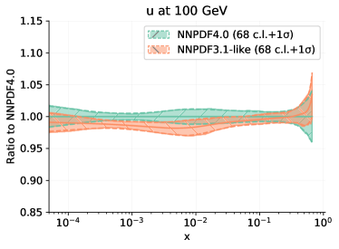
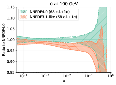
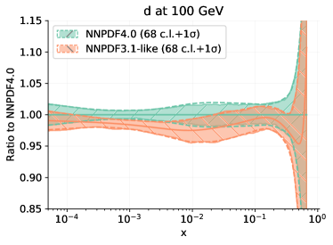
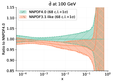
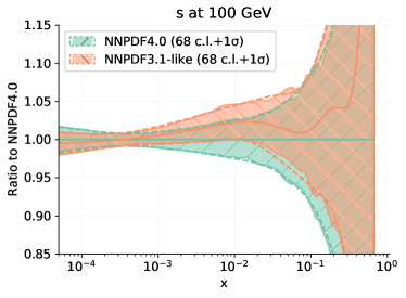
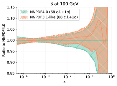
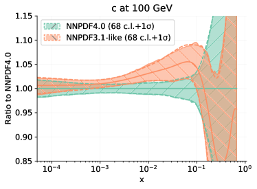
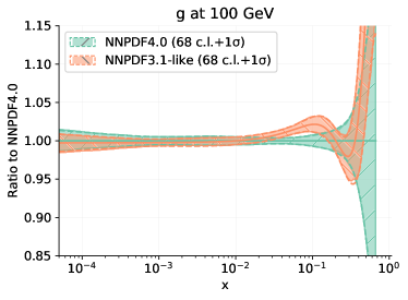
Figure 7.3: Same as Fig. 7.1 now comparing to the NNPDF4.0 baseline a PDF set based on the same NNPDF4.0 methodology but on the NNPDF3.1-like dataset defined in Sect. 2.1.

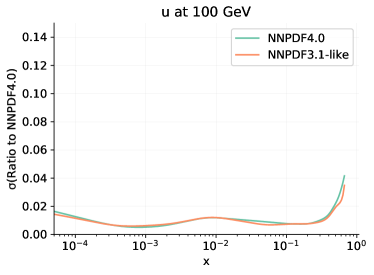
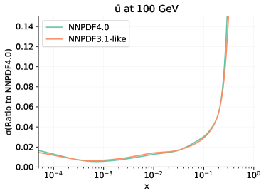
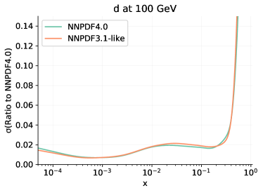
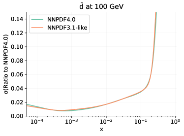
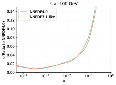
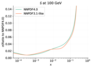
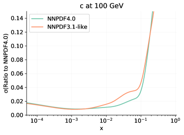
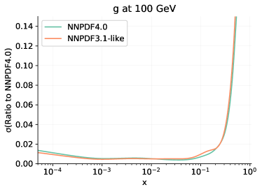
Figure 7.4: Same as Fig. 7.3 but for one-sigma relative uncertainties.

Interestingly, even though there is compatibility within uncertainties, the central values of all PDFs change, often almost at the one-sigma level, with the largest differences seen in the gluon, as noted in Sect. 5.2.1. This means that the new data are bringing in new experimental information. In the case of the light quark and antiquark PDFs, the new data (mostly from LHC inclusive gauge boson production, as we will see in Sect. 7.2.1) produce an enhancement of up to 3% for $0.01\lesssim x\lesssim 0.1$ of the up and down PDFs, and a milder suppression of the strange PDF. In the case of charm, a suppression of about 4-5% is seen for $0.01\lesssim x\lesssim 0.1$ and an enhancement of about 10% for $x\gtrsim 0.1$. In the case of the gluon, the impact (mostly from single-inclusive jet and dijet production, as we will see in Sect. 7.2.3) is a suppression of about 2-3% around $x\sim 0.1$ and a similar enhancement around $x\sim 0.3$.

While shifts of central values are typically of the size of the PDF uncertainties, it is clear from Fig. 7.4 that the uncertainties themselves are unchanged, except possibly for a reduction of the uncertainty in charm in the region $0.01\lesssim x\lesssim 0.1$. On the other hand, comparing to the PDFs determined using the NNPDF3.1-like dataset and methodology, Fig. 7.2, one observes that the pattern in change of central values is the same. Therefore we conclude that the differences in the shape of PDFs between NNPDF3.1 and NNPDF4.0 are mostly data-driven, but with little or no impact on uncertainties. It follows that when comparing to the published NNPDF3.1, the overall effect of the new data is to improve the accuracy of the parton set while not significantly affecting its precision.

7.2 PDFs from reduced datasets

We now discuss a number of PDF sets determined by removing specific measurements from the baseline, with the goal of assessing their impact. We consider in turn: LHC inclusive gauge boson production; LHC single top-quark and SeaQuest data; LHC jet, top pair, $Z$ $p_{T}$, and direct photon; all the LHC data altogether; collider data; and DIS data.

7.2.1 The impact of LHC inclusive gauge boson production data

In the global fit, quark flavor separation is driven by charged-current DIS structure functions and by inclusive gauge boson production in hadronic collisions. In the latter case, the bulk of the data comes from the LHC. The ATLAS and CMS data are mostly in the central rapidity region, sensitive to quarks and antiquarks in the intermediate-$x$ region, while the LHCb data cover the forward rapidity region, sensitive to quarks and antiquarks at large $x$ and small $x$.

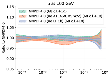
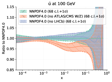
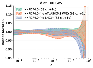
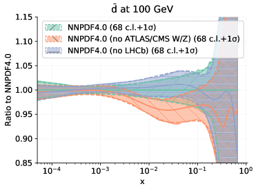
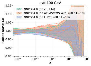
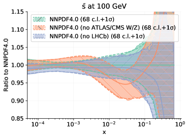
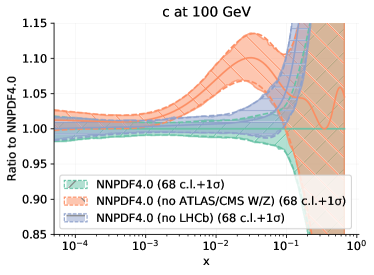
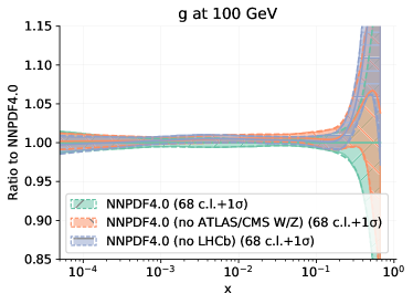
Figure 7.5: Same as Fig. 7.1 comparing the baseline to PDFs determined removing either all of the ATLAS and CMS, or all of the LHCb inclusive gauge boson production data.

In order to assess the impact of this data we have produced two PDF sets removing from the baseline all of the inclusive gauge boson production measurements, either from ATLAS and CMS, or from LHCb. Fig. 7.5 compares these PDFs to the baseline. The effect of removing the ATLAS and CMS data is a suppression of the light quarks and antiquarks (by 2-4%) and an enhancement of the charm (by up to 10%) around $0.01\lesssim x\lesssim 0.1$. The effect of removing the LHCb data is more moderate and predominately affects the down, charm and gluon at around $x\gtrsim 0.1$. Specifically, the former is suppressed while the latter two are enhanced in comparison to the baseline (in both cases by up to 10%). The shift of central values is generally within the PDF uncertainty, except for the up, antiup, antidown and charm when excluding the ATLAS and CMS data, and for the down quark when excluding LHCb data. As expected, and as mentioned in Sect. 7.1.2, this data is thus responsible for the bulk of the changes in light quark PDFs between NNPDF3.1 and NNPDF4.0.

7.2.2 The impact of LHC single-top production data and of SeaQuest data

Additional constraints on quark flavor separation at large $x$, in particular on the $d/u$ and $\bar{d}/\bar{u}$ ratios, are in principle provided by single top-quark production at the LHC and by fixed-target DY production recently measured by the SeaQuest experiment. Because these measurements are included for the first time in NNPDF4.0 (see Sects. 2.2.9 and 2.2.3) it is interesting to study their impact. To this purpose, we have produced two PDF sets, respectively removing from the baseline either all of the single top data, or the SeaQuest measurement.

In Fig. 7.6 we compare the $d/u$ and $\bar{d}/\bar{u}$ ratios, at $Q=10$ GeV; in the former case we show results obtained from the fit without single top data, and in the latter we show results obtained omitting SeaQuest data, both compared to the NNPDF3.1 and NNPDF4.0 baselines.

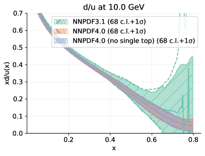
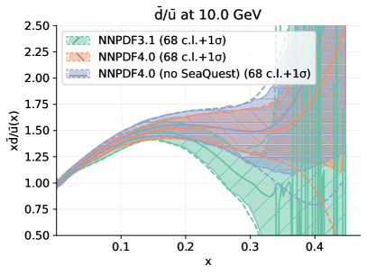
Figure 7.6: The $d/u$ (left) and $\bar{d}/\bar{u}$ (right) ratios, at $Q=10$ GeV, computed, respectively, from a NNPDF4.0 fit without single top-quark data or without SeaQuest data. In both cases we show results obtained with the NNPDF3.1 and NNPDF4.0 baseline fits.

Single-top data have essentially no impact on the $d/u$ ratio and more generally on the whole PDF determination. This is due to the relatively large experimental uncertainties of the corresponding measurements, as already noted in Sect. 5.1 and in Ref. [8]. The significant reduction in uncertainty on the $d/u$ ratio between NNPDF3.1 and NNPDF4.0 is methodology-driven, as we will show explicitly in Sect. 8 below. Indeed, we will show (see Fig. 8.2) that the uncertainty on the large-$x$ up and down quark distributions is significantly reduced when switching from NNPDF3.1 to NNPDF4.0 methodology with fixed NNPDF4.0 data, while we have seen (compare Fig. 7.4) that the same uncertainty is essentially unchanged when reducing the dataset to the NNPDF3.1 one with fixed NNPDF4.0 methodology. It is interesting to note that the expectation for the $d/u$ ratio seems to converge to a finite value between 0 and 1. This result may be used to discriminate non-perturbative models of nucleon structure [228].

The SeaQuest data have a moderate impact on the $\bar{d}/\bar{u}$ ratio, and essentially no impact on other PDFs. They lead to a moderate reduction in the PDF uncertainty, but they leave the baseline central value almost unchanged. In comparison to NNPDF3.1, the $\bar{d}/\bar{u}$ ratio is enhanced by 50% around $x\sim 0.3$ but remains compatible with the larger NNPDF3.1 uncertainties. We therefore conclude that the SeaQuest data have very little impact on NNPDF4.0 due to their overall consistency with other data. Interestingly, the $\bar{d}/\bar{u}$ ratio in NNPDF4.0 differs somewhat from that in NNPDF3.1, due to the updated flavor separation driven by the gauge boson production data discussed in Sect. 7.2.1. The SeaQuest data thus provide, for the particular case of the $\bar{d}/\bar{u}$ ratio, an independent confirmation of the improved knowledge on flavor separation obtained in NNPDF4.0 thanks to LHC data.

7.2.3 The impact of LHC jet, top-quark pair, $Z$ $p_{T}$ and direct photon data

Various LHC processes in the NNPDF4.0 dataset constrain the gluon PDF: top pair and single-inclusive jet or dijet production, at large values of $x$; and $Z$ $p_{T}$ and direct photon production at intermediate values of $x$. In order to assess the impact of these measurements, we have produced four fits by removing each of them in turn from the baseline.

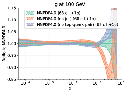
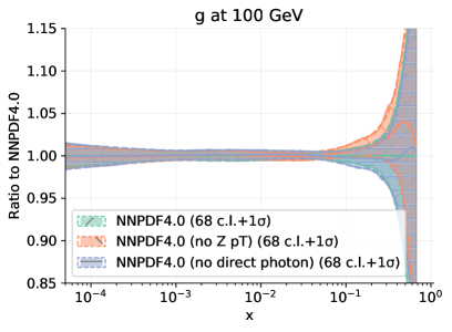
Figure 7.7: The gluon PDF obtained removing single-inclusive jet and dijet data or top pair data (left), or $Z$ $p_{T}$ data or direct photon data (right).

In Fig. 7.7 we compare to the baseline the gluon from each of these determinations. All other PDFs are essentially unaffected by these changes in dataset, with only small changes in the quark PDFs when removing the jet observables. For clarity, we display separately PDFs without top pair production and jet data, and PDFs without $Z$ $p_{T}$ and direct photon data. Only the gluon PDF is shown, normalized to the central value of the NNPDF4.0 baseline.

The effect of the data is hierarchical. Single-inclusive jet and dijet data have the largest impact: if they are removed, the gluon is slightly enhanced (by 2-3%) around $0.01\lesssim x\lesssim 0.1$ and then more strongly suppressed (by up to 15%) for $x\gtrsim 0.1$. This suggests that the other datasets, specifically top pair data, tend to pull in the opposite direction, suppressing somewhat the gluon at large $x$. Top pair data have a moderate impact: if they are removed, the gluon is slightly enhanced for $x\gtrsim 0.1$, but within the baseline uncertainty. $Z$ $p_{T}$ data have a yet smaller impact: if they are removed, the gluon is again a little enhanced for $x\gtrsim 0.1$. The size of this shift is smaller than that observed in the case of the fit without top-quark pair data and it remains compatible with baseline uncertainty. Direct photon data have no effect: if they are removed, the gluon does not change at all.

These results indicate that single-inclusive and dijet production data, which are the most abundant and precise, drive the features of the gluon in the global fit. Other data provide some generally consistent and complementary information, particularly the top pair production data.

7.2.4 The impact of LHC data

It is clear from Sects. 7.2.2-7.2.3 that the impact of LHC data on NNPDF4.0 is non-negligible. In order to assess their cumulative effect, we have produced a PDF set by removing all of the LHC measurements. Fig. 7.8 compares this PDF set to the baseline. It is clear that the LHC data have a substantial impact, both on central values and uncertainties: PDF central values change by up to two sigma in the region $0.01\lesssim x\lesssim 0.4$. This change is qualitatively similar to, but rather more significant than, the change when removing LHC data from NNPDF3.1 (see Sect. 4.10 in Ref. [5]). The change in central value is well within the PDF uncertainty in the large-$x$ region, $x\gtrsim 0.4$, except for the charm PDF. We conclude that NNPDF4.0 PDFs are significantly more accurate than PDFs obtained omitting LHC data, except at very large-$x$, where the loss of precision may be not greater than the loss of accuracy.

It is clear that the role of the LHC data has now substantially changed in comparison to PDFs determined before the LHC Run II. Indeed, for NNPDF3.0 the impact of the LHC data was still moderate, and subdominant in comparison to that of the combined HERA data (see in particular Sect. 5.2.2 of Ref. [14]).

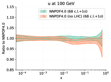
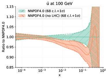
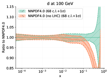
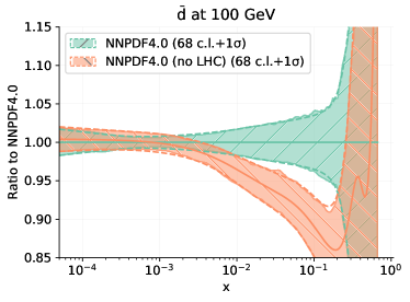
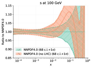
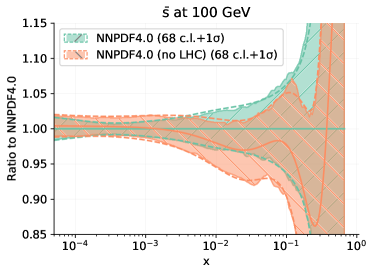
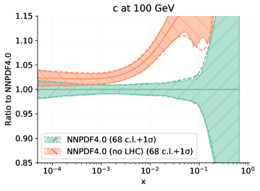
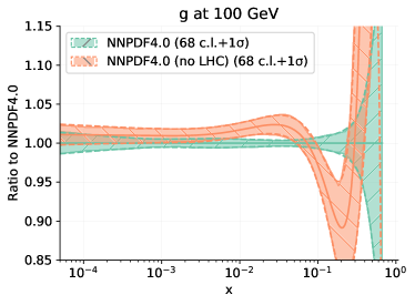
Figure 7.8: Same as Fig. 7.1 now comparing the baseline to PDFs determined removing from the dataset all LHC data.

7.2.5 The impact of collider data

We have previously [229, 14, 5] suggested that collider-only PDFs could be more accurate than global PDFs: retaining only collider data excludes low-energy datasets, which may be subject to potentially large perturbative and non-perturbative corrections, and datasets for which the reliability of experimental uncertainties has sometimes been questioned. However, in the NNPDF3.1 analysis (see Sect. 4.12 in Ref. [5]) it was observed that in practice collider-only PDFs are not competitive due to their very large uncertainties: the increase in uncertainty when fitting only collider data was generally much larger than the change in central value, thus suggesting that the loss of precision was much greater than any possible gain in accuracy.

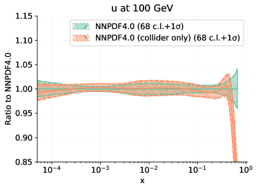
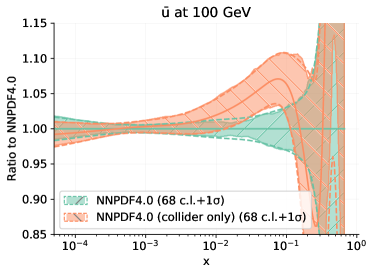
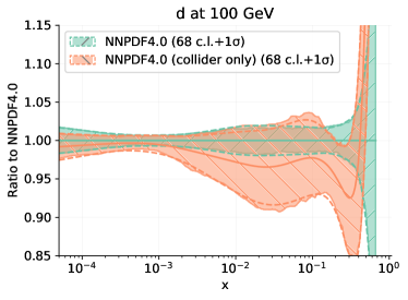
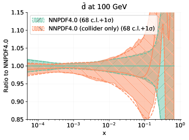
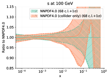
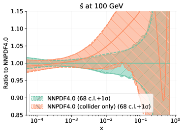
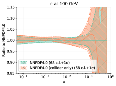
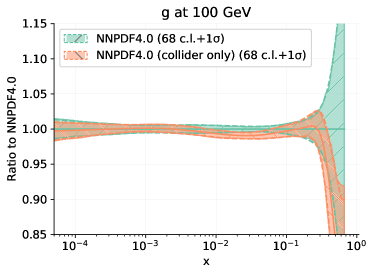
Figure 7.9: Same as Fig. 7.1 now comparing the baseline to PDFs determined excluding all fixed-target data from the dataset (collider-only PDFs).

We revisit this state of affairs in the context of NNPDF4.0, where the amount of LHC data has been significantly expanded. The collider-only PDFs are compared to the baseline in Fig. 7.9. It is clear that now, unlike in the case of NNPDF3.1, some PDFs are almost as precise in the collider only and global fit: this is the case for the up, charm, and gluon. However, there is still a very considerable loss of precision on the other PDFs at large $x$, most likely due to the impact of neutrino data and of data with deuterium targets on the down and strange quark and antiquark PDFs. We conclude that even though we are approaching a situation in which collider-only PDFs might be competitive, we are not quite there yet.

7.2.6 The impact of DIS data

Deep-inelastic scattering measurements have provided the bulk of the experimental information in global fits for a long time, and DIS-only PDFs have been widely used as a possibly more accurate and only marginally less precise alternative to global fits. As with collider-only PDFs, the situation is now worth revisiting. To this purpose, we have produced a PDF determination in which only DIS data are retained; and one in which all the HERA data are removed from the dataset. They are compared to the baseline in Fig 7.10.

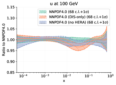
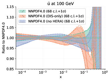
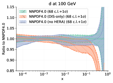
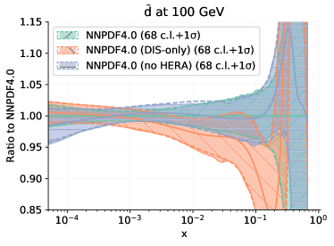
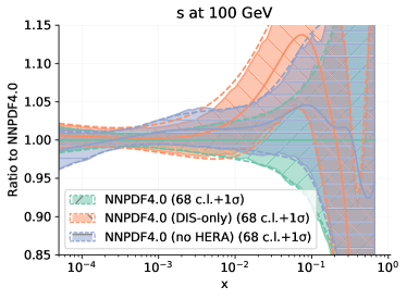
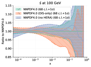
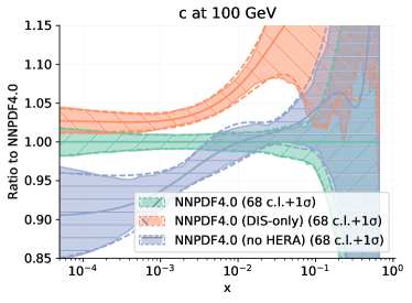
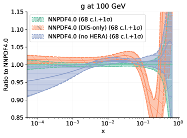
Figure 7.10: Same as Fig. 7.1 now comparing the baseline to PDFs determined from DIS data only, or removing all HERA data.

Comparing the DIS-only PDFs to the baseline, large differences are seen, for both central values and uncertainties. It is only in the small $x$ region, where quark PDFs are controlled by the mixing of the dominant singlet component with the gluon, that there is good agreement between DIS-only and global PDFs. The only PDFs which remain essentially unchanged are the strange quark and antiquark. This confirms the key role played by neutrino DIS (dimuon) data in constraining them.

Interestingly however, the no-HERA PDFs are in perfect agreement with the baseline, with only a moderate increase in uncertainty, with the exception of charm. This means that whereas the small-$x$ behavior of the gluon and singlet determined from HERA is in agreement with that coming from the LHC data, the HERA data are no longer required in order to determine the correct behavior of PDFs at small $x$. An exception is charm, which at small $x$ is constrained by the combined HERA $\sigma_{\rm NC}^{c}$ data. As mentioned in Sect. 4.2.4 this is the reason why this data is retained in the baseline, despite its poor fit quality, which is possibly due to missing higher order corrections.

We conclude that on the one hand, unlike in previous NNPDF determinations, for NNPDF4.0 it is no longer true that a DIS-only fit is competitive, and on the other hand the HERA data are no longer needed in order to fix the small $x$ behavior of PDFs (with the exception of charm). This is consistent with our previous conclusion in Sect. 7.2.4 that the NNPDF4.0 PDF determination is largely controlled by LHC data.

7.3 PDFs from extended datasets

We now discuss a number of PDF sets determined by adding specific measurements to the baseline. We consider in turn: the ATLAS 8 TeV $W^{\pm}$ lepton rapidity distributions [81]; the EMC charm structure function data [44]; the 7 TeV ATLAS and CMS single-inclusive jet data [75, 147] (in lieu of dijets); the NOMAD neutrino dimuon data [111]; and the HERA single-inclusive and dijet data [112, 113, 115, 116]. In the last two cases, the impact of the additional measurements is studied by means of Bayesian reweighting [155, 156], for the reasons explained in Sect. 2, starting from a prior PDF ensemble of 1000 replicas.

7.3.1 The ATLAS 8 TeV $W^{\pm}$ data

As discussed in Sect. 4, the ATLAS measurement of the 8 TeV lepton rapidity differential cross-section for $W^{\pm}$ production [81] is not included in the baseline dataset because it does not pass our selection criteria. Nevertheless we study its impact by performing a fit in which it is added to the NNPDF4.0 baseline dataset. It turns out that the impact on PDFs of these data is tiny. The down and strange antiquarks are the most affected: their central values are respectively suppressed and enhanced by half a sigma in the region $0.01\lesssim x\lesssim 0.1$. The PDFs, normalized to the central value of the NNPDF4.0 baseline, are displayed at $Q=100$ GeV in Fig. 7.11. We conclude that this dataset is in fact consistent with the baseline, and its pathological behavior upon being given a large weight is likely related to its poorly behaved covariance matrix. This will be shown to be indeed the case in Sect. 8.7 below. A poor fit quality to this dataset was also found in the MSHT20 analysis [144].

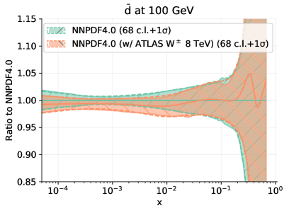
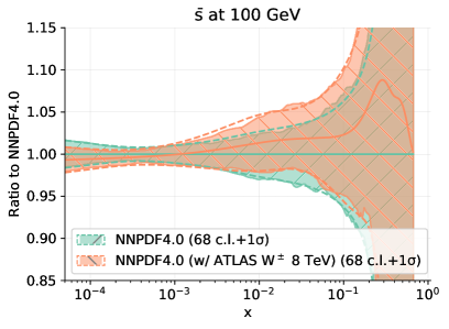
Figure 7.11: Comparison to the baseline of the antidown and antistrange PDFs obtained adding to the baseline the ATLAS lepton rapidity distributions from $W^{\pm}$ production at 8 TeV [81].

7.3.2 The EMC charm structure function data

In previous NNPDF studies [230, 5], it was found that EMC charm structure function data [44] significantly reduce the uncertainty on the charm PDF at large $x$, which in this region, upon inclusion of this data, deviates significantly from the result (compatible with zero) of perturbative matching, and exhibits a behavior similar to models of intrinsic charm [231]. These data however have not been included in the baseline because the reliability of the EMC estimate of systematic uncertainties has been questioned, even though not for this specific measurement (see Refs. [230, 232] for details). We revisit this issue here by adding the EMC data to the baseline dataset. Furthermore, nuclear uncertainties related to the use of a Fe target are now taken into account following the procedure explained in Sect. 2.3.

A good fit quality is obtained overall and specifically for the EMC measurement, with a value of the $\chi^{2}$ of 0.62. The charm PDFs for this determination is compared to the baseline in Fig. 7.12 (left) at $Q=1.65$ GeV, just above the charm threshold. Remarkably, the inclusion of this data leaves the central charm PDF unchanged: there is perfect consistency between the EMC data and the global dataset. Thanks to this consistency, a reduction of the charm PDF uncertainty is found around $x\sim 0.03$ and $x\sim 0.3$, by a moderate amount. A much more significant uncertainty reduction upon the inclusion of the EMC data was observed in Ref. [5] (see Sect. 4.9). This means that the extension of the dataset from NNPDF3.1 to NNPDF4.0 leads to a charm PDF whose uncertainty is greatly reduced, and whose central value is in perfect agreement with that determined by the EMC data.

These findings suggests that the NNPDF4.0 analysis favors a non-zero intrinsic charm component in the proton. A more quantitative assessment of this statement requires however a determination of the PDFs in the $n_{f}=3$ scheme, which is left to future studies [233].

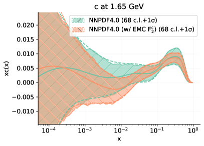
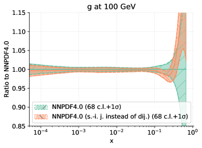
Figure 7.12: (Left) Comparison to the baseline of the charm PDF at $Q=1.65$ GeV from a determination in which the EMC charm structure function data  [44] are included. (Right) The gluon PDF at $Q=100$ GeV compared and normalized the baseline from a determination replacing 7 TeV ATLAS and CMS dijet data with single-inclusive jets.

7.3.3 ATLAS and CMS single-inclusive jet data

In Sect. 4.3 as a part of dataset selection we had to choose between single-inclusive jets and dijets, given that the lack of information on their correlation prevents their simultaneous inclusion. Whereas we concluded that 8 TeV CMS dijet data has potential issues and thus decided in favor of the inclusion of single-inclusive jets, for 7 TeV data we concluded that the single-inclusive jets and dijets are consistent and we decided for the inclusion of dijets due to the fact that the dijet observable is favored theoretically [137, 9].

We now consider a variant of the baseline in which the 7 TeV dijet data are replaced by single-inclusive jets. In the case of the ATLAS data, we decorrelate systematic uncertainties across different rapidity bins according to the procedure recommended in [88]. Results remain unchanged if we include any of the individual rapidity bins, as we had already observed in the context of NNPDF3.1 [234]. The fit quality is as good as the baseline, with statistically equivalent PDFs. The gluon from this set is compared to the baseline in Fig. 7.12 (right). We observe a mild distortion of the large-$x$ shape: a slight suppression around $x\simeq 0.3$ followed by an enhancement at larger $x$, well within the PDF uncertainty. We thus confirm compatibility between jets and dijets at 7 TeV.

7.3.4 The NOMAD neutrino dimuon data

As discussed in Sect. 7.2.6, the strange quark PDF is mostly constrained by the neutrino-DIS charm dimuon data from NuTeV. LHC data, namely $W$ and $Z$ boson production, possibly in association with jets, provide additional, consistent constraints. In Ref. [10], the NOMAD measurement [111] of the dimuon to inclusive neutrino-nucleus CC DIS cross-section ratio, $\mathcal{R}_{\mu\mu}$, was shown to further pin down the uncertainty of the strange quark PDF.

Here we assess whether or not the same conclusion holds within the reduced uncertainties of the NNPDF4.0 determination. To this purpose, we repeat the reweighting analysis of Ref. [10], but now starting from the NNPDF4.0 baseline as a prior. No nuclear corrections are taken into account, despite the fact that the NOMAD experiment utilized a Fe target, as nuclear corrections cancel in the cross-section ratio measured by this experiment (see Ref. [10]). We find that the NOMAD data are very well described by the NNPDF4.0 prior before reweighting: the $\chi^{2}$ per data point is equal to 0.66. The impact of the data is therefore expected to be limited. After reweighting, the $\chi^{2}$ improves to 0.61. The number of effective replicas is $N_{\rm eff}=622$, out of $N_{\rm rep}=1000$ in the prior set. The strange quark PDF, the only one to to be affected, is displayed before and after reweighting in Fig. 7.13 (left). It is clear that the NOMAD data leave unchanged the central value and only contribute to a moderate uncertainty reduction in the region around $x\sim 0.1$. Similar conclusions can be drawn from the comparison of the ratio $\mathcal{R}_{\mu\mu}$ as a function of the neutrino energy $E_{\nu}$, also shown in Fig. 7.13 (right).

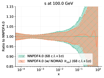
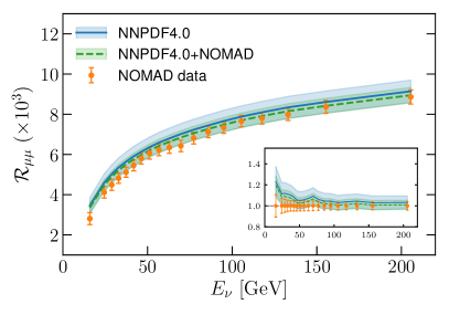
Figure 7.13: (Left) Comparison between the baseline and PDFs in which the NOMAD neutrino DIS data are included by reweighting. The strange PDF is shown at $Q=100$ GeV. (Right) The same comparison for the measured ratio $\mathcal{R}_{\mu\mu}$ as a function of the neutrino energy $E_{\nu}$. The inset displays quantities normalized to the central experimental value.

7.3.5 The HERA DIS jet data

Additional constraints on the gluon are provided by deep-inelastic jet production. We study the impact of the selection of available measurements performed by ZEUS and H1 discussed in Sect. 2.2.2, by means of Bayesian reweighting, for the reasons discussed there. All the datasets are included at once in the reweighting; results are given in Table 7.1, where for each dataset we give the number of data points and the $\chi^{2}$ value before and after reweighting, along with the total $\chi^{2}$ values for the full DIS jet dataset. Experimental correlations between single-inclusive jet and dijet production measurements are taken into account whenever provided (specifically for Refs. [115, 116]). However, because DIS jet data are included via reweighting, their correlations with the inclusive DIS data used in the baseline fit cannot be included. This is a partial limitation of the reweighting analysis.

The number of effective replicas after reweighting is $N_{\rm eff}=530$, out of $N_{\rm rep}=1000$ in the prior set. In Fig. 7.14 we compare the reweighted gluon PDF to the baseline NNPDF4.0 result, shown as a ratio to the latter at $Q=100$ GeV. We show both the central gluon obtained when reweighting with each of the datasets listed in Table 7.1 (left) and the central value and uncertainty obtained when reweighting with the full set of DIS jet data (right). Single-inclusive jet and dijet measurements from H1 (separately for low-$Q$ and high-$Q$) are considered as a single dataset, given that experimental correlations are completely known.

	ZEUS 820 (HQ) (1j)	ZEUS 920 (HQ) (1j)	H1 (LQ) (1j)	H1 (HQ) (1j)	ZEUS 920 (HQ) (2j)	H1 (LQ) (2j)	H1 (HQ) (2j)	Total DIS+jets
$N_{\rm dat}$	30	30	48	24	22	48	24	226
$\chi^{2}$ (NNPDF4.0, before reweighting)	0.96	1.75	1.86	1.78	1.82	1.62	1.98	1.80
$\chi^{2}$ (NNPDF4.0, after reweighting)	0.96	1.45	1.59	1.62	1.67	1.53	1.65	1.68

Table 7.1: The number of data points $N_{\rm dat}$ and the $\chi^{2}$ value before and after reweighting the NNPDF4.0 baseline PDF set with the full set of DIS jet data (see Sect. 2.2.2 for details). The total $\chi^{2}$ values are also shown.

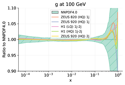
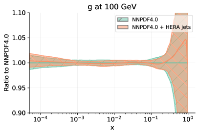
Figure 7.14: The gluon PDF obtained reweighting the NNPDF4.0 baseline with DIS jet data, shown as a ratio to the former at $Q=100$ GeV. We show the central gluon obtained when reweighting with each of the DIS jet data of Table 7.1 in turn (left), and the central gluon and uncertainty obtained when reweighting with the full DIS jet dataset considered here (right).

It is clear that the impact of the DIS jet data is very moderate. Indeed, the fit quality of this data is already quite good before their inclusion and does not change substantially: this is also apparent from the small reduction of the effective number of replicas upon reweighting. We conclude that this data is consistent with the baseline and, if fully included in the baseline dataset would not affect significantly the outcome of the PDF determination.

8 Methodology dependence and stability

After assessing, in the previous section, the impact of the new data on NNPDF4.0, we now turn to the corresponding assessment of the impact of the new methodology. This has the dual aim of, on the one hand, complementing the analysis of the previous section and providing a full understaning of the differences between NNPDF4.0 and previous PDF sets, specifically NNPDF3.1, and on the other hand, providing detailed tests of the stability and robustness of our results.

We first assess the impact of the new NNPDF4.0 methodology, by comparing PDF sets based on the same underlying dataset, but using either the new NNPDF4.0 or the previous NNPDF3.1 methodology. We then study specifically the impact of the new positivity and integrability constraints, respectively discussed in Sect. 3.1.3 and Sect. 3.1.4. Next, we then turn to the explicit demonstration of the independence of results on the choice of parametrization basis of Sect. 3.1.1, we discuss the impact of independently parametrizing the charm PDF (which is the NNPDF default since NNPDF3.1), and we study the impact of the new implementation of nuclear corrections presented in Sect. 2.3. Finally, we study the possibility of regularizing the covariance matrix for datasets for which it is poorly conditioned, and use the result to reassess the impact of some of the problematic datasets considered in Sect. 4.2.4.

8.1 Impact of the NNPDF4.0 methodology

We complement the comparison between NNPDF3.1 and NNPDF4.0 presented in Sect. 7.1.2, where the impact of the NNPDF4.0 dataset was analyzed, by now studying the impact of the NNPDF4.0 methodology. This is done by comparing to the NNPDF4.0 baseline a PDF set determined from the NNPDF4.0 dataset, but using NNPDF3.1 methodology. Results are shown in Figs. 8.1-8.2.

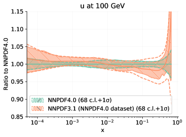
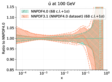
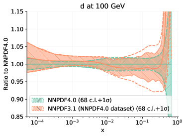
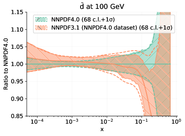
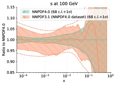
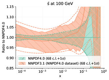
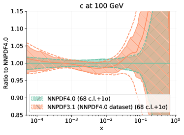
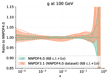
Figure 8.1: Same as Fig. 7.3 but now presenting the complementary comparison of the baseline of PDFs to a set based on the same NNPDF4.0 dataset, but using the old NNPDF3.1 methodology.

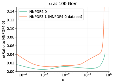
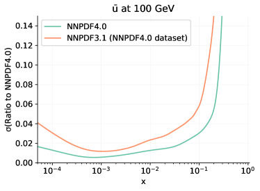
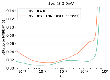
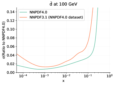
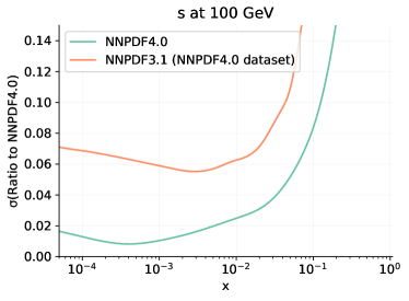
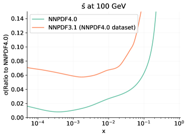
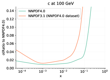
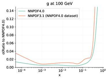
Figure 8.2: Same as Fig. 8.1 but showing the one-sigma relative uncertainties.

It is clear that PDFs obtained by the two methodologies are in perfect agreement: given a common dataset, the NNPDF4.0 and NNPDF3.1 methodologies produce consistent results. This confirms the conclusions of Sect. 6, where the two methodologies were compared specifically in the framework of closure and future tests. However, it is clear that the NNPDF4.0 methodology leads to significantly more precise results, as is apparent from Fig. 8.2. This also agrees with the conclusions of Sect. 6: the old and new methodology are both faithful (accurate within their stated precision), but the new methodology is more precise.

Putting this together with the results of Sect. 7.1.2 we conclude that the change in PDF central values from NNPDF3.1 to NNPDF4.0 is due to the much expanded dataset, especially because of LHC data, but the reduction in uncertainty is almost entirely due to the improved methodology.

8.2 Impact of PDF positivity

As discussed in Sect. 3.1.3, strict positivity of the gluon and the light quarks and antiquarks PDFs is enforced in NNPDF4.0, based on the results of Ref. [21]. This implies that there is an extra set of positivity constraints, on top of those that were already implemented in NNPDF3.1 where positivity of several observables or pseudo-observables (such as DIS structure functions for individual quark flavors) was required. In order to assess the impact of these new PDF positivity constraints, we have produced a PDF determination in which only the previous NNPDF3.1 positivity constraints are implemented, while everything else is identical to the NNPDF4.0 baseline in terms of both data and methodology.

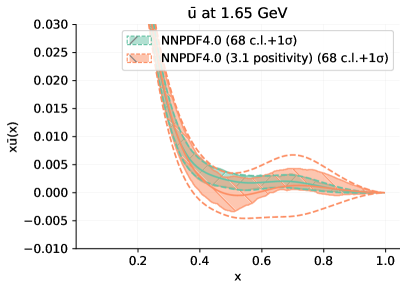
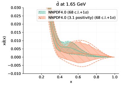
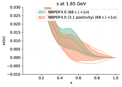
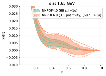
Figure 8.3: Comparison to the baseline NNPDF4.0 fit of the PDFs determined by removing the new PDF positivity constraints, and hence using only the NNPDF3.1 positivity conditions. The antiup, antidown, strange and antistrange PDFs are shown at the input parametrization scale $Q=1.65$ GeV.

In Fig. 8.3 we compare to the NNPDF4.0 baseline fit some of the ensuing PDFs: we show the antiup, antidown, strange and antistrange at the parametrization scale $Q=1.65$ GeV. It is clear that the new PDF positivity constraints have a substantial impact in the large-$x$ region, $x\gtrsim 0.3$, both in terms of reducing the uncertainty and of preventing PDF replicas from going negative. This latter property ensures positivity of cross-sections for the production of final states even for very large invariant masses $m_{X}$.

8.3 Impact of nonsinglet integrability

As explained in Sect. 3.1.4, in NNPDF4.0 additional integrability constraints are added to those already implemented in NNPDF3.1. First, integrability of the Gottfried and strangeness sums, i.e. integrability of $T_{3}$ and $T_{8}$, is imposed through Lagrange multipliers. Second, the range of preprocessing exponents is determined self-consistently as for NNPDF3.1, but it is no longer allowed to extend into the non-integrable region. Finally, integrability is imposed at the post-fit selection level. This ensures that all replicas remain integrable, so nonsinglet sum rules are finite and with finite uncertainty.

We assess the impact of these new integrability constraints by comparing to the NNPDF4.0 baseline the PDFs obtained by removing both of them, i.e. with no Lagrange multipliers for $T_{3}$ and $T_{8}$ and unconstrained preprocessing range, and the PDFs determined by keeping the constraint on the preprocessing range but removing the Lagrange multipliers for $T_{3}$ and $T_{8}$.

In Fig. 8.4 we compare the PDFs obtained in this way to the NNPDF4.0 baseline: we show the $T_{3}$ and $T_{8}$ nonsinglet PDFs at the parametrization scale $Q=1.65$ GeV. It is clear that the effect of the new constraints is seen only in the small $x\lesssim 10^{-3}$ region, where there is limited experimental information on quark flavor separation (see Fig. 2.1). The effect of the new integrability constraints is significant for $T_{3}$, but moderate for $T_{8}$: in particular, $T_{8}$ remains integrable even when both constraints are removed, while integrability of $T_{3}$ is enforced when constraining the preprocessing, but would otherwise fail. The effect of the Lagrange multiplier is mostly to reduce somewhat the small-$x$ uncertainties by removing some outliers. It is important to note, however, that these constraints can be rather more significant when PDFs are determined from a restricted dataset, such as those considered in Sect. 7. Indeed, inspection of $T_{8}$ in the no-LHC and DIS-only fits respectively discussed in Sect. 7.2.6 and 7.2.4 shows a rather different small-$x$ behavior and larger uncertainties, that could well extend into the nonintegrable region in the absence of an explicit constraint.

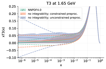
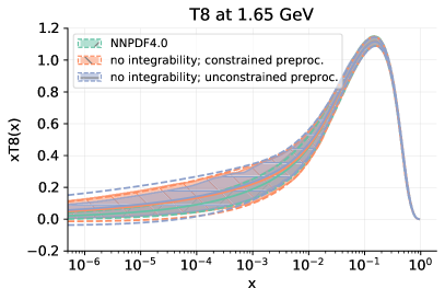
Figure 8.4: Comparison to the baseline of PDFs obtained removing either or both the new integrability constraints on the triplet and octet PDFs (see text). The triplet $T_{3}$ and octet $T_{8}$ are shown at $Q=1.65$ GeV.

It is interesting to compare these results to those of the CT18 and MSHT20 determinations, shown in Fig. 8.5. In the case of the triplet $T_{3}$, the central CT18 and MSHT20 $xT_{3}$ PDF combination also vanishes as $x\to 0$, but for MSHT20 the uncertainty band extends into the nonvanishing (positive) range. In the case of the octet, for both CT18 and MSHT20 $xT_{8}$ does not vanish as $x\to 0$, resulting in substantially larger PDF uncertainties for light flavor separation in the small-$x$ region.

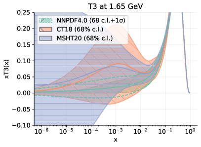
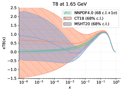
Figure 8.5: Same as Fig. 8.4 now comparing the NNPDF4.0 baseline to CT18 and MSHT20.

8.4 Parametrization basis independence

As discussed in Sect. 3.1, in the NNPDF4.0 determination the PDFs are parametrized by default in the evolution basis at the input scale $Q_{0}=1.65$ GeV. This means that the eight neurons of the final layer of the neural network displayed in Fig. 3.9 correspond to the eight basis PDFs $f_{k}$ listed in Eq. (3.4), up to preprocessing and normalization prefactors as given in Eq. (3.5). However, results should be completely independent of this basis choice. An alternative option, also discussed in Sect. 3.1, is to use the flavor basis, in which the eight neurons of the final layer now correspond instead to the eight basis PDFs $\tilde{f_{k}}$ of Eq. (3.3). The results of a global PDF analysis should in principle be the same irrespective of whether PDFs are parametrized in the evolution basis, Eq. (3.1), or in the flavor basis, Eq. (3.3), or indeed in any other basis.

To demonstrate explicitly that this is the case for NNPDF4.0, we have carried out a PDF determination in the flavor basis. This is a significant modification of the fitting methodology, so the hyperoptimization procedure has been repeated. The final methodology settings in this case are provided in Table 3.3, along with the baseline (evolution basis) settings. The ensuing PDFs are compared to the baseline in Fig. 8.6. PDFs are not shown in the far small-$x$ extrapolation region where, as discussed in Sect. 3.1.1, the behavior of flavor-basis PDFs is the superposition of different powers and cannot be preprocessed as in the evolution basis, and hence the corresponding integrability constraints cannot be enforced, see Sects. 3.1.4 and 8.3.

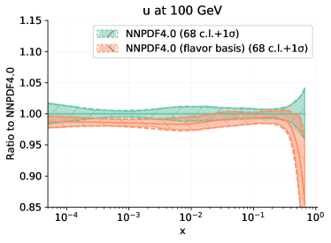
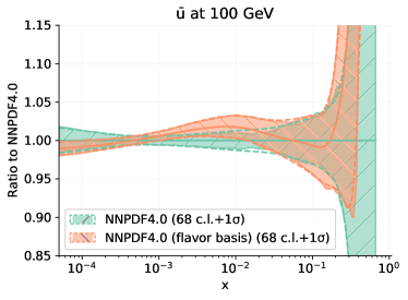
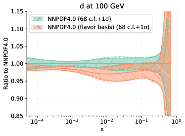
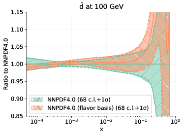
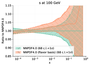
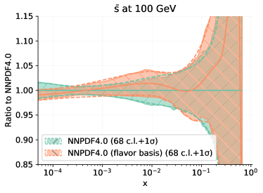
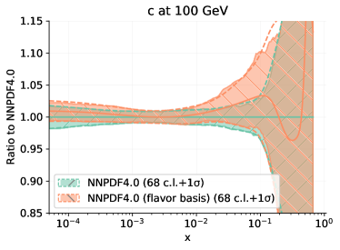
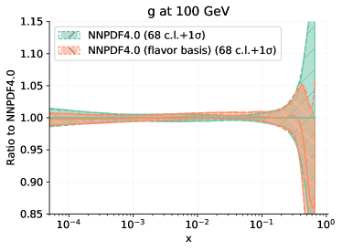
Figure 8.6: Same as Fig. 7.3, but now comparing the baseline PDFs, parametrized in the evolution basis, to PDFs parametrized in the flavor basis and determined with the corresponding hyperparameter settings of Table 3.3.

It is clear from Fig. 8.6 that PDFs in the two bases are in excellent agreement, with differences fully compatible within the PDF uncertainties. It is important to understand that the results obtained from a flavor basis parametrization correspond to an entirely new methodology: specifically, as discussed in Sect. 3.1 they do not contain any small–$x$ preprocessing, and indeed this requires a considerably larger neural net architecture, compare the first and third column in Tab. 3.3. Hence we do not expect them to be trivially identical to those obtained from the evolution basis parametrization, but rather statistically compatible with them, as it is indeed the case. We have in fact verified that if we combine replicas obtained using the flavor basis and evolution basis parametrization in a single replica set uncertainties are essentially unchanged, thus confirming compatibility of the two results.

The flavor basis parametrization is more unstable due to the need of using a larger neural network architecture, and it becomes unreliable at small $x$ because of the difficulty of enforcing the correct subleading Regge behavior, as discussed in Sect. 3.1. Therefore, we have not pursued the flavor basis parametrization further for the sake of precision phenomenology. However, the results presented here demonstrate independence of the choice of the parametrization and provide a highly nontrivial test of the robustness of the NNPDF4.0 framework.

8.5 Treatment of the charm PDF

Since the NNPDF3.1 analysis, in the NNPDF baseline fits the charm PDF is parametrized alongside the light quark PDFs. This has various advantages, specifically in absorbing into the initial PDF possible higher-order contributions to perturbative matching conditions, thereby greatly reducing the dependence of results on the value of the charm mass [230], and also allowing for a possible non-perturbative intrinsic charm component.

Here we assess the impact of parametrizing charm by comparing the baseline PDFs to PDFs in which charm is determined using standard NNLO perturbative matching. The fit quality deteriorates somewhat, with the total $\chi^{2}$ per data point increasing from the value 1.16 of Table 5.1 to 1.18. The datasets that show a more marked deterioration are gauge boson production and deep-inelastic scattering, which are those most sensitive to quark flavor decomposition.

The PDFs obtained when charm is determined by perturbative matching are compared to the baseline in Fig. 8.7. Results are qualitatively similar to those already observed when the same comparison was performed in NNPDF3.1 [5]. It is particularly interesting to note the stability of the gluon PDF, which in the perturbative charm approach is directly responsible for driving the charm PDF. Light quark PDFs are generally larger at small $x\lesssim 0.003$ and smaller at larger $x\sim 0.1$ when charm is not parametrized. The charm PDF is of course most affected, with the PDF, when parametrized, being rather larger at large $x\gtrsim 0.1$, smaller for $0.01\mathrel{\hbox to0.0pt{\lower 4.0pt\hbox{\hskip 1.0pt$\sim$}\hss}\raise 1.0pt\hbox{$<$}}x\mathrel{\hbox to0.0pt{\lower 4.0pt\hbox{\hskip 1.0pt$\sim$}\hss}\raise 1.0pt\hbox{$<$}}0.1$, and then larger again for $2\times 10^{-4}\mathrel{\hbox to0.0pt{\lower 4.0pt\hbox{\hskip 1.0pt$\sim$}\hss}\raise 1.0pt\hbox{$<$}}x\mathrel{\hbox to0.0pt{\lower 4.0pt\hbox{\hskip 1.0pt$\sim$}\hss}\raise 1.0pt\hbox{$<$}}0.01$ as compared to its perturbatively determined counterpart. Note however that if charm is not parametrized, its value in the region $0.01\mathrel{\hbox to0.0pt{\lower 4.0pt\hbox{\hskip 1.0pt$\sim$}\hss}\raise 1.0pt\hbox{$<$}}x\mathrel{\hbox to0.0pt{\lower 4.0pt\hbox{\hskip 1.0pt$\sim$}\hss}\raise 1.0pt\hbox{$<$}}0.1$ depends very strongly on the value of the charm mass $m_{c}$.

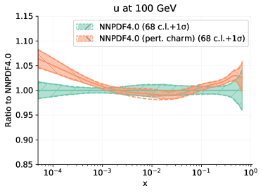
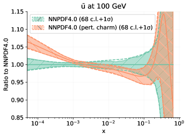
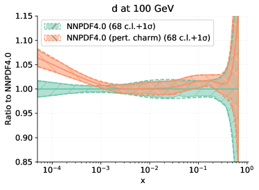
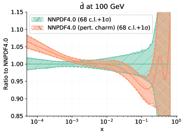
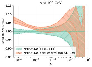
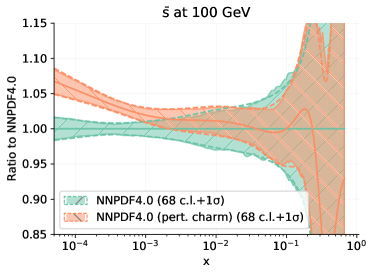
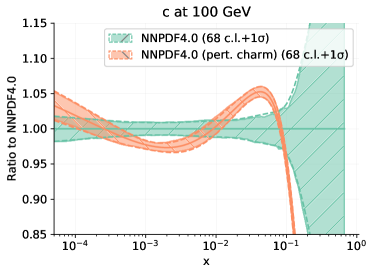
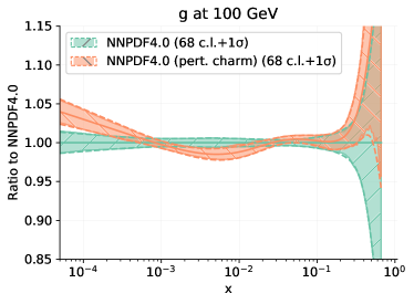
Figure 8.7: Same as Fig. 7.3, comparing to the baseline PDFs in which charm is not independently parametrized but rather determined by perturbative matching. The charm mass is taken to be $m_{c}=1.51$ GeV in both fits.

It is interesting to observe that the uncertainties of all PDFs other than charm are quite similar whether or not charm is parametrized. In fact, in several cases, such as the gluon at small $x\mathrel{\hbox to0.0pt{\lower 4.0pt\hbox{\hskip 1.0pt$\sim$}\hss}\raise 1.0pt\hbox{$<$}}10^{-3}$ and light antiquark PDFs at intermediate $x\mathrel{\hbox to0.0pt{\lower 4.0pt\hbox{\hskip 1.0pt$\sim$}\hss}\raise 1.0pt\hbox{$<$}}0.1$, the PDF uncertainties are actually smaller when charm is parametrized. This demonstrates the improved overall consistency of the global PDF determination when charm is parametrized. Of course, the uncertainty on the charm PDF itself is significantly larger when it is parametrized.

The charm PDF at the parametrization scale of $Q_{0}=1.65$ GeV is directly compared in Fig. 8.8 to its perturbatively generated counterpart, along with the gluon PDF that drives the latter. The stability of the gluon PDF can be directly appreciated, in particular for $x\mathrel{\hbox to0.0pt{\lower 4.0pt\hbox{\hskip 1.0pt$\sim$}\hss}\raise 1.0pt\hbox{$>$}}10^{-3}$. The charm PDF, when independently parametrized, displays clear evidence for a valence-like component at low scales and for $x\mathrel{\hbox to0.0pt{\lower 4.0pt\hbox{\hskip 1.0pt$\sim$}\hss}\raise 1.0pt\hbox{$>$}}0.1$, with a statistical significance approaching the $3\sigma$ level, while in the $x\mathrel{\hbox to0.0pt{\lower 4.0pt\hbox{\hskip 1.0pt$\sim$}\hss}\raise 1.0pt\hbox{$<$}}0.1$ region it is consistent with zero within uncertainties. The shape of the perturbatively generated charm is very different, and its very small uncertainty (which does not include the charm mass uncertainty or missing higher order corrections) looks unrealistic.

We conclude that parametrizing charm has a moderate but non-negligible effect, especially on the light flavor separation, and it improves the overall fit quality and consistency. The best-fit parametrized charm displays evidence for a valence-like component at large $x$ and low scale, which could be identified with an intrinsic charm component of the proton. A dedicated investigation of this issue will be presented in a follow-up publication [233].

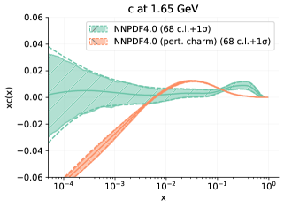
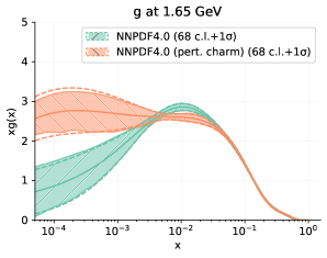
Figure 8.8: Same as Fig. 8.7 for the gluon and the charm PDFs at the parametrization scale $Q=1.65$.

8.6 Impact of nuclear corrections

As discussed in Sect. 2.3, the baseline NNPDF4.0 determination includes nuclear uncertainties as an extra contribution to the covariance matrix, both for data taken on deuteron and heavy nuclei targets. The impact of these corrections is assessed here. To this purpose, we have produced dedicated PDF sets with different settings for the treatment of deuteron and heavy nuclear uncertainties, summarized in Table 8.1. These correspond to including nuclear effects in either the default way, as additional theory uncertainties (denoted as “unc”), or in the alternative way briefly discussed in Sect. 2.3 in which they are included as a correction to the experimental data, with a correspondingly reduced uncertainty, (denoted as “shift”) or not at all, for either or both deuterium or heavy nuclei.

The values of the $\chi^{2}$ per data point, for each process type and for the complete dataset, for each of these PDF determinations are collected in Table 8.1. The value of the $\phi$ estimator (as defined in Eq. (4.6) of Ref. [14], also equal to the square-root of the variance Eq. (6.8)) is also given. This is a measure of the (correlated) PDF uncertainty in units of the data uncertainty. A graphical representation of the results of Table  8.1 is provided in Fig. 8.9, where all datasets that are unaffected by nuclear corrections are grouped as in the “other” category.

Upon including nuclear uncertainties, the $\chi^{2}$ for the global fit improves rather significantly, from 1.27 to 1.17. This better fit quality can be traced to the improved description of the fixed-target CC DIS and Drell-Yan datasets, with similar outcomes for the “unc” and “shift” options. This decrease in $\chi^{2}$ may look unsurprising, since an extra source of uncertainty is being added, which affects around one third of the global dataset. However, note that the $\phi$ estimator is almost unchanged: this means that PDF uncertainties remain almost the same. The lowest total $\chi^{2}$ value is found for the baseline fit. Indeed, the reduction in $\chi^{2}$ is a little more marked when nuclear corrections are added as an extra uncertainty, rather than a shift. In the latter case, the extra contribution to the uncertainty only corresponds to the uncertainty in the shift itself. This suggests that the baseline treatment of nuclear corrections as uncertainties is a little more conservative than the shift option. The reduction in $\chi^{2}$ from the fit with no nuclear corrections to the baseline is roughly the sum of the decreases observed when either the deuteron or the heavy nuclear datasets are corrected.

	No nucl. unc.	Deut. unc.	Deut. shift	HeavyN unc.	HeavyN shift	Shift	NNPDF4.0
DIS NC (fixed-target)	1.27	1.27	1.27	1.26	1.27	1.26	1.26
DIS CC (fixed-target)	0.86	0.86	0.86	0.86	0.87	0.86	0.86
DIS NC (collider)	1.20	1.19	1.19	1.19	1.19	1.19	1.19
DIS CC (collider)	1.27	1.299	1.29	1.26	1.25	1.28	1.28
Drell-Yan (fixed-target)	0.94	0.93	0.92	1.00	1.01	0.96	0.98
Tevatron $W,Z$ prod. (incl.)	1.22	1.25	1.27	1.15	1.14	1.12	1.10
LHC inclusive $W,Z$ prod. (incl.)	1.51	1.49	1.48	1.40	1.40	1.37	1.37
LHC $W,Z$ production ($p_{T}$ and jets)	1.13	1.14	1.14	1.14	1.14	1.14	1.14
LHC top-quark pair production	1.23	1.21	1.20	1.18	1.20	1.18	1.20
LHC jet production	1.30	1.27	1.26	1.30	1.30	1.25	1.26
LHC isolated $\gamma$ production	0.74	0.74	0.73	0.77	0.76	0.76	0.76
LHC single $t$ production	0.36	0.37	0.36	0.37	0.36	0.36	0.36
Total $\chi^{2}$	1.27	1.25	1.25	1.19	1.21	1.19	1.17
Total $\phi$	0.15	0.16	0.16	0.16	0.16	0.16	0.16

Table 8.1: The value of the $\chi^{2}$ per data point for the NNPDF4.0 baseline and its variants with different treatments of nuclear corrections. Values are shown for each process type and for the complete dataset. The value of the $\phi$ estimator for the complete dataset is also provided (see text).

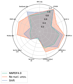
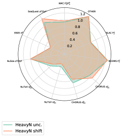
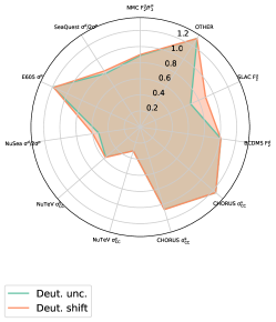
Figure 8.9: The values of the $\chi^{2}$ for individual datasets for the PDF fits listed in Table 8.1. The datasets unaffected by nuclear corrections are grouped in the “other” category.

The effect of nuclear corrections on PDFs is non-negligible, in particular in the large-$x$ region. In Fig. 8.10 the antiup and antidown PDFs at $Q=30$ GeV determined without nuclear corrections, or with heavy nuclear corrections only, are compared to the baseline (with the default treatment of nuclear corrections). Inclusion of nuclear corrections leads to an increase in uncertainty at large $x\mathrel{\hbox to0.0pt{\lower 4.0pt\hbox{\hskip 1.0pt$\sim$}\hss}\raise 1.0pt\hbox{$>$}}0.2$, and also a different shape, with in particular a significant enhancement around $x\simeq 0.5$. Heavy nuclear corrections have the largest impact, especially on the antidown PDF. Nevertheless, all PDFs agree well within their respective uncertainty bands. This suggests that neglecting deuteron and heavy nuclear uncertainties could distort the determination of the sea quark PDFs at large-$x$.

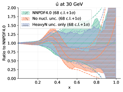
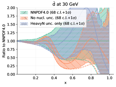
Figure 8.10: The antiup and antidown PDFs at $Q=30$ GeV from the “No nucl. unc.” and “HeavyN unc.” PDF sets of Tab. 8.1 compared to the baseline.

PDFs obtained with either of the two alternative treatments of nuclear corrections are compared in Fig. 8.11. First (top), we compare to the baseline the antiup and antidown PDFs as in Fig. 8.10 but now with all nuclear and deuterium corrections included as shifts, and then (bottom) we compare directly the antiup PDF when either the deuterium or the nuclear corrections are included with either the uncertainty or the shift method. It is clear that the impact of the nuclear corrections on the PDF with either method is quite similar, the only difference being that uncertainties are somewhat smaller when the shift method is adopted. This is in agreement with the behavior of the $\chi^{2}$ values observed previously, and confirms that the baseline prescription is somewhat more conservative.

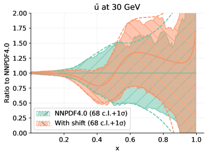
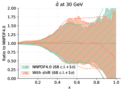
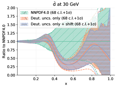
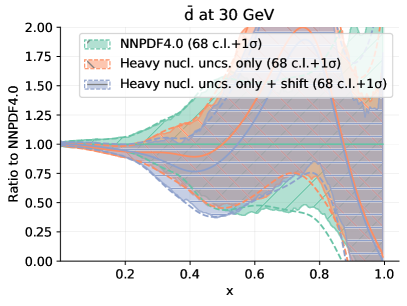
Figure 8.11: Top: same as Fig. 8.10, but now with PDFs from the “Shift” set. Bottom: comparison to the baseline of the antidown PDF at $Q=30$ from the “Deut Unc” and “Deut shift” sets (left) or from the “HeavyN unc” and the “HeavyN shift” sets (right).

As mentioned in Sect. 2.3, the evaluation of the deuterium corrections with the method of Ref. [19] requires a self-consistent determination of the deuterium PDF, which has been performed here starting with the NNPDF4.0 set and then proceeding as was done in Ref. [19] for NNPDF3.1. A byproduct of this procedure is then, of course, an independent determination of the deuterium PDFs and thus of deuterium structure functions, with corresponding correlated uncertainties, which we now discuss briefly.

In Fig. 8.12 we display the $F_{2}^{d}/F_{2}^{p,0}$ structure function ratio at $Q$ = 10 GeV, where by $F_{2}^{p,0}$ we denote the isospin singlet component of the proton structure function, so $F_{2}^{d}/F_{2}^{p,0}=1$ in the absence of nuclear corrections. The associated one-sigma PDF uncertainty band is also shown, with correlations between deuteron and proton PDFs taken into account. The results from the nNNPDF2.0 nuclear PDF fit and from a phenomenological determination in MSHT20 [144] are also shown for comparison.

The deuteron corrections to $F_{2}^{d}/F_{2}^{p,0}$ are seen in Fig. 8.12 to be quite small, as expected since the deuteron is a loosely bound nucleus. The three estimates for $F_{2}^{d}/F_{2}^{p,0}$ are consistent with each other and agree within uncertainties. In all three cases, one finds that the correction is only important at large-$x$, with a dip of a couple percent for $x\simeq 0.4$ and then an enhancement at larger values of $x$. The uncertainties for the NNPDF4.0-based determination are slightly larger in the low-$x$ region, reflecting that this determination is a somewhat more conservative. This determination also has the smallest correction factor, which is in general very close to one except for $x\mathrel{\hbox to0.0pt{\lower 4.0pt\hbox{\hskip 1.0pt$\sim$}\hss}\raise 1.0pt\hbox{$>$}}0.6$.

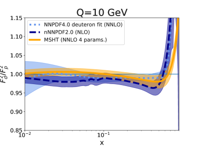
Figure 8.12: The ratio of deuteron to the iso-singlet proton structure functions, $F_{2}^{d}//F_{2}^{p,0}$, evaluated using the proton and deuteron PDFs obtained in the present NNPDF4.0 analysis at $Q=10$ GeV as a function of $x$. Results are compared to the nNNPDF2.0 nuclear PDF fit and the phenomenological correction factor from MSHT20.

8.7 Regularized covariance matrices

The selection procedure of Sect. 4 revealed that several of the datasets considered as potential candidates for the inclusion in the global PDF analysis exhibit a large value of the stability metric $Z$, Eq. (4.2), which may lead to artificially high $\chi^{2}$ values due to ill-defined covariance matrices. As discussed there, the value of $(\sqrt{2}Z)^{-1}$ can be interpreted as the precision at which correlations need to be estimated in order to ensure that they affect the $\chi^{2}$ by less than one standard deviation. This implies e.g. that a dataset with $Z=10$ requires correlations to be estimated with an absolute uncertainty of less than $0.07$, else the $\chi^{2}$ will be inflated. The potentially problematic nature of publicly released experimental covariance matrices is sometimes acknowledged by the experimental collaborations, and alleviated by their provision of alternative decorrelation models characterized by a different pattern of correlated systematics.

The stability analysis carried out in Sect. 4 focused on the impact of large weight fits at the PDF level, and based on the results of these fits, it established which datasets were suitable for inclusion in the baseline dataset, essentially by making sure that they would not distort the global fit. Here we assess the effect on the global PDF fit when datasets exhibiting large values of $Z$ have their covariance matrices regularized by means of a tailored procedure. For datasets that we did decide to include in NNPDF4.0, the purpose of this is to confirm that our best-fit PDFs are indeed not distorted by the inclusion of this data. For datasets that were not included, the aim is to assess what would be their impact if it was possible to safely include them.

The decorrelation procedure that we apply here is described in more detail in Ref. [205]. It is based on clipping the eigenvectors until a target value of the stability metric, $Z_{\rm reg}$, is achieved. For instance, if the target value is chosen to be $Z_{\rm reg}=4$, then the clipping algorithm transforms the original experimental correlation matrix into a different matrix with the same eigenvectors as the original one but such that the eigenvalues that were smaller than $1/Z_{\rm reg}^{2}=1/16$ are replaced by 1/16. The motivation for this decorrelation procedure is to give a decorrelated covariance matrix which is as close as possible to the original one provided by the experiments. This is in contrast to other approaches such as adding a small diagonal contribution, or varying ad hoc the pattern of correlations for specific sources of systematic uncertainties.

Dataset	$N_{\rm dat}$	$Z_{\rm orig}$	$\chi^{2}_{\rm orig}$	$\chi^{2}_{\rm reg}$
ATLAS $W,Z$ 7 TeV CC ($\mathcal{L}=4.6$ fb-1)	46	9.01	1.89	0.93
ATLAS $W$ 8 TeV (*)	22	11.28	3.50	1.15
CMS dijets 7 TeV	54	4.70	1.81	1.73
ATLAS dijets 7 TeV	90	9.93	2.14	0.92
CMS 3D dijets 8 TeV (*)	122	4.47	1.50	0.92

Table 8.2: The values of the $\chi^{2}$ in NNPDF4.0 variants in which the covariance matrices for selected datasets have been regularized following the procedure discussed in the text. For each dataset, we indicate the number of data points, the original values of the fit quality $\chi^{2}_{\rm orig}$ and of the stability metric $Z_{\rm orig}$, and then the values of the $\chi^{2}_{\rm reg}$ obtained by repeating the fit with the regularized covariance matrix for this dataset, for a choice of the target metric of $Z_{\rm reg}=4$. Datasets denoted by (*) are not part of the baseline and have been obtained from dedicated PDF fits (see text).

We have repeated the global NNPDF4.0 NNLO determination, but now regularizing in turn the covariance matrix of those datasets that exceeded the threshold value of the stability metric (See Tabs. 4.2-4.5 in Sect. 4), with the threshold value $Z_{\rm reg}=4$ now chosen as target clipping value. Results are shown in Table 8.2: in each case we display the number of data points, the value of $Z$ for the given experiment before regularization ($Z_{\rm orig}$), and the $\chi^{2}$ for the experiment before and after regularization. Note that, based on the dataset selection procedure of Sect. 4, the ATLAS $W$ 8 TeV and CMS 3D dijets 8 TeV datasets are not part of the NNPDF4.0 baseline. In the former case, the regularization has been applied to a dedicated PDF determination in which the ATLAS data have been added to the baseline. In the latter case, the regularization has been applied to the the PDF determination shown in Table 4.7, “CMS 3D dijets 8 TeV” entry. All other datasets listed in Table 8.2 are already part of the baseline. It is clear from Table 8.2 that after regularization all $\chi^{2}$ values are of order unity, with the possible exception of CMS 7 TeV dijets. Note that the improvement in the values of the $\chi^{2}$ is not driven by an increase in the diagonal elements of the covariance matrix, which remains smaller than 5%, but rather from the regularization of the smallest eigenvectors. It thus amounts to a minimal modification of the covariance matrix.

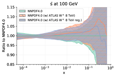
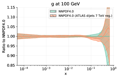
Figure 8.13: Comparison to the baseline of PDFs obtained by regularizing the covariance matrix for the ATLAS $W$ 8 TeV (left) and ATLAS 7 TeV dijet dataset (right). In each case, the PDF which is most affected is shown: antistrange (left) and gluon (right). In the left plot both the default baseline and a baseline with the unregularized data are shown.

Interestingly, one also finds that the best-fit PDFs are left almost unchanged by the regularization procedure. Specifically, in Fig. 8.13 we compare PDFs obtained regularizing the ATLAS $W$ 8 TeV (left) and ATLAS 7 TeV dijet data (right) to the baseline PDFs. In the former case, since the ATLAS $W$ 8 TeV are not part of the default dataset, we show both the default baseline, and a modified version in which this data has been added in unregularized form. In each case, we show the PDF that is most affected by the regularization, respectively the antistrange and the gluon. It is clear that, despite the large differences at the $\chi^{2}$ level, the regularization procedure leaves the PDFs mostly unaffected. This said, the effects of regularization are not completely negligible in all cases: for example, for the ATLAS 7 TeV dijets at $x\simeq 0.2$ the gluon PDF is suppressed by around one-sigma as compared to the baseline in the regularized fits. Nevertheless, these remain quite moderate effects, a feature which might appear somewhat counterintuitive given the large reduction in the $\chi^{2}$ values.

Our general conclusion is that a poor $\chi^{2}$ does not necessarily imply a genuine inconsistency, since it can arise from ill-defined (unstable) covariance matrices. The specific conclusion for the datasets that have been examined here is that we observe almost no difference between PDFs determined with and without regularizing the corresponding covariance matrices. For the datasets that we retained in the baseline dataset, this analysis confirms that the global fit is not distorted by the poorly behaved nature of their covariance matrices.

For the two datasets that we did not retain, the situation is somewhat different. In the case of the ATLAS $W$ 8 TeV data shown in Fig. 8.13, there is essentially no difference between PDFs determined including or not including this dataset in regularized or unregularized form. For the CMS 3D 8 TeV dijets, we see no difference between PDFs determined with regularized or unregularized covariance matrix, but both differ significantly from the baseline, as discussed in Sect. 4.3. Hence, in both cases the poor $\chi^{2}$ is due to the properties of the covariance matrix, and we confirm our decision not to include these datasets in the baseline: in the former case on the grounds that it would make no difference, and in the latter case for the reasons discussed in Sect. 4.3.

9 Phenomenology

We present a first study of the implications of the NNPDF4.0 PDFs for hadron collider phenomenology. Specifically, we compare the PDF luminosities at $\sqrt{s}=14$ TeV from NNPDF4.0 to other available PDF sets, and we then present theoretical predictions obtained using these PDF sets for representative LHC inclusive cross-sections and differential distributions. Specifically, we consider inclusive gauge boson production, Higgs boson production in different channels, and top quark pair production. As we shall see, PDF uncertainties found using NNPDF4.0 are typically of the order of one percent for a broad range of observables and in a wide kinematic region.

9.1 PDF luminosities

We evaluate here PDF luminosities for different parton initial state combinations. We consider the parton luminosities as a function of the invariant mass of the final state $m_{X}$, both integrated over rapidity and differential in rapidity, as defined in Eqs. (1-4) of Ref. [235].

In Fig. 9.1 we compare the luminosities integrated over rapidity, computed at $\sqrt{s}=14$ TeV using NNPDF4.0 and NNPDF3.1 PDFs, as a function of the final-state invariant mass $m_{X}$. For each parton combination, we show the ratio to the central NNPDF4.0 and the relative one-sigma PDF uncertainty. Then in Fig. 9.2 percentage uncertainties on the parton luminosities differential in rapidity are shown as a two-dimensional contour plot as a function of the invariant mass $m_{X}$ and rapidity $y$ of the final state. In this case, we also show for reference the up-antidown luminosity (relevant e.g. for $W^{+}$ production).

The first obvious observation is the significant reduction of PDF uncertainties that was already observed in Sect. 5.2. Indeed, it is clear, especially from Fig. 9.2, that the uncertainty is now around 1% in a wide kinematic region and for several parton channels. In terms of overall compatibility, all luminosities agree at the one sigma level. While central values for the quark-gluon and quark-antiquark luminosities are almost unchanged, the quark-quark luminosity is somewhat enhanced and the gluon-gluon luminosity somewhat suppressed in NNPDF4.0 compared to NNPDF3.1, in the region $m_{X}\lesssim 3$ TeV.

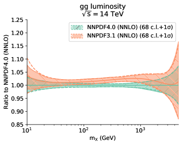
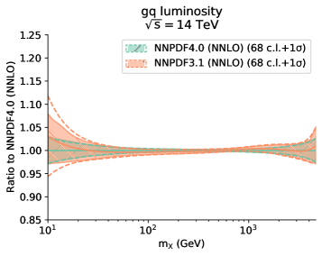
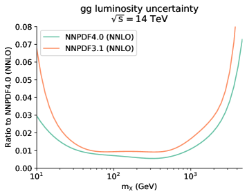
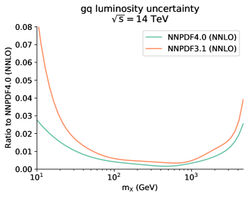
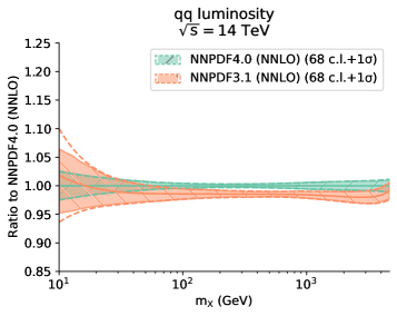
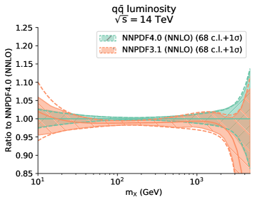
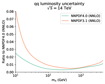
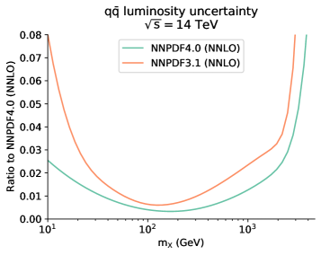
Figure 9.1: Comparison, as a function of the invariant mass $m_{X}$, of the parton luminosities at $\sqrt{s}=14$ TeV computed using NNLO NNPDF4.0 and NNPDF3.1 PDFs, where the luminosities have been integrated over the final-state rapidity $y$. The ratio to the NNPDF4.0 central value and the relative one-sigma uncertainty are shown for each parton combination.

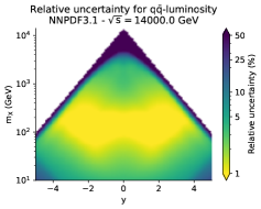
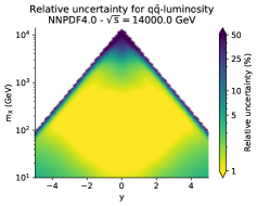
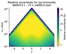
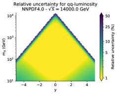
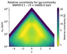
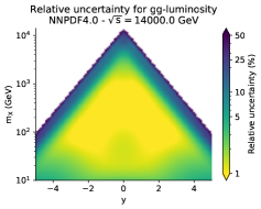
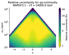
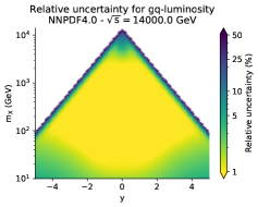
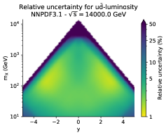
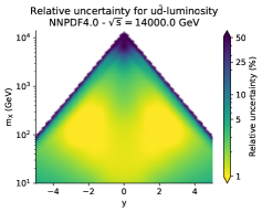
Figure 9.2: The relative uncertainty on the parton luminosities of Fig. 9.1, now plotted as a function of the invariant mass $m_{X}$ and the rapidity $y$ of the final state; the left plots show results for NNPDF3.1 and the right plots for NNPDF4.0; results for the up-antidown luminosity are also shown in the last row.

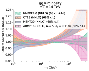
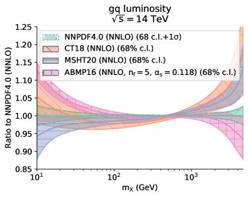
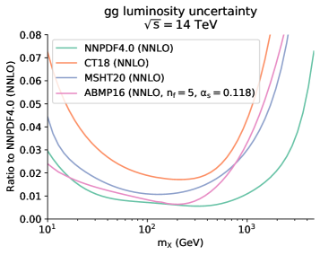
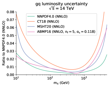
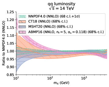
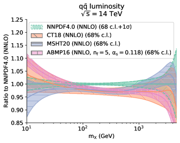
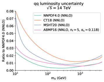
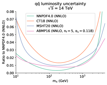
Figure 9.3: Same as Fig. 9.1 but now comparing NNPDF40, ABMP16, CT18, and MSHT20 PDFs.

We next compare the NNPDF4.0 luminosities integrated in rapidity to those obtained using PDFs from the CT18 [143], MSHT20 [144] and ABMP16 [142] sets. When comparing uncertainties, it should be kept in mind that while CT18, MSHT20 and ABMP16 all adopt a Hessian methodology with a fixed functional form, their respective treatments of uncertainties differ. Specifically, both CT18 and MSHT20 adopt a “tolerance” [208, 236] criterion and further study functional form dependence in order to span adequately the space of parametrizations, while ABMP do not. Hence, CT18 and MSHT20 uncertainties are directly comparable to those of NNPDF (which adopts a very general neural network parametrization), while ABMP uncertainties generally are not. The same common value of $\alpha_{s}(m_{Z})=0.118$ is used in all cases. Note that this significantly differs from the value $\alpha_{s}(m_{Z})=0.113$ adopted as default in Ref. [142]. Again as already observed in Sect. 5.2, it is clear that NNPDF4.0 generally has the smallest uncertainty. An exception is ABMP16 in some regions (such as the gluon-gluon luminosity for low invariant mass), possibly for the reason mentioned above (as already pointed out in Ref. [5].

All luminosities agree within uncertainties in the region around $m_{X}\sim 100$ GeV, relevant e.g. for Higgs and gauge boson production. Furthermore, the quark-quark and quark-antiquark luminosity are in good agreement within uncertainties over the full mass range. For the gluon sector luminosities (gluon-gluon and gluon-quark), however, differences are seen at large mass. Specifically, in the high-mass region, $m_{X}\mathrel{\hbox to0.0pt{\lower 4.0pt\hbox{\hskip 1.0pt$\sim$}\hss}\raise 1.0pt\hbox{$>$}}1$ TeV, the gluon-gluon and quark-gluon luminosities for NNPDF4.0 are rather smaller than MSHT20 and CT18, though they agree with ABMP16. These differences are possibly a consequence of the fact that NNPDF4.0 includes a variety of data which are sensitive to the gluon and are not used by other groups, in particular the dijet cross-sections at 7 TeV and the $t\bar{t}$ differential distributions from the LHC Run II.

A full understanding of the origin of the differences between PDFs determined by different groups and their impact on LHC phenomenology would require a dedicated benchmark study, such as the ones carried out for the PDF4LHC15 [237] and PDF4LHC21 [214, 215] combinations for NNPDF3.0 and NNPDF3.1 respectively. In the remainder of this section, we will assess how these differences at the level of parton luminosities translate into LHC cross-sections and distributions.

9.2 Inclusive cross-sections

We present theory predictions for representative LHC processes, first for integrated cross-sections and then for the corresponding differential distributions, based on the luminosities discussed in Sect. 9.1. In all cases, realistic acceptance requirements and final state kinematic cuts are imposed, in order to provide theoretical predictions which are as close as possible to the associated experimental measurements. All cross-sections are evaluated at $\sqrt{s}=14$ TeV.

We consider the following processes: neutral and charged current Drell–Yan production in the leptonic final state, top pair production, gauge boson pair production (both in the $\mathrm{W}^{+}\mathrm{W}^{-}$ and the $\mathrm{W}^{\pm}\mathrm{Z}$ channels), inclusive Higgs production via gluon fusion or vector boson fusion, and the associated production of Higgs and $\mathrm{W}^{\pm}$. Note that some of these processes are already part of the NNPDF4.0 determination, but at a different center-of-mass energy: specifically, neutral current (dilepton) Drell–Yan production and top pair production data are included for center-of-mass energies of $7$, $8$ and $13$ TeV.

Calculational settings.

Results presented in this section have been produced using MadGraph5_aMC@NLO [125, 124] and account for complete NLO corrections both in the QCD and electroweak couplings. These mg5_aMC calculations have been interfaced to PineAPPL [16], which produces interpolation grids so that the LHC predictions can be quickly evaluated for arbitrary PDF sets without redoing the MC integration. In the specific case of top pair production, our calculation include only the $\mathcal{O}(\alpha_{\mathrm{s}}^{2})$ and $\mathcal{O}(\alpha_{\mathrm{s}}\alpha)$ terms at LO and the $\mathcal{O}(\alpha_{\mathrm{s}}^{3})$ and $\mathcal{O}(\alpha_{\mathrm{s}}^{2}\alpha)$ corrections at NLO. This is justified since the pure-EW and mixed corrections that we neglect, namely $\mathcal{O}(\alpha^{2})$, $\mathcal{O}(\alpha_{\mathrm{s}}\alpha^{2})$ and $\mathcal{O}(\alpha^{3})$, are very small in the kinematic regions under consideration [238].

For electroweak gauge boson production, we account for their decays into leptons. In order to simplify the calculation, we choose the flavors of these final-state leptons to be different from each other, so as to minimize the number of Feynman diagrams. This, for example, avoids the overlap of $\mathrm{Z}\mathrm{Z}$ with $\mathrm{W}^{+}\mathrm{W}^{-}$ diboson production, both of which can decay into the $\ell\bar{\ell}\nu_{\ell}\bar{\nu}_{\ell}$ final state, while only the later can decay into the $\ell\bar{\ell}^{\prime}\nu_{\ell^{\prime}}\bar{\nu}_{\ell}$ final state, which is the one we have selected.

For all calculations except Higgs production, we use the model loop_qcd_qed_sm_Gmu with enabled complex-mass scheme [239, 240, 241] as implemented by Ref. [124]. For Higgs production we use the UFO model of [242, 243] with an effective Higgs–gluon–gluon coupling, for which EW corrections vanish. The following are taken as independent input parameters:

$$m_{\mathrm{W}} =80.352~{}{\rm GeV}\text{,} \Gamma_{\mathrm{W}} =2.084~{}{\rm GeV}\text{,} m_{t} =172.5~{}{\rm GeV}\text{,}$$ (9.1)

$$m_{\mathrm{Z}} =91.1535~{}{\rm GeV}\text{,} \Gamma_{\mathrm{Z}} =2.4943~{}{\rm GeV}\text{,} \Gamma_{t} =1.37758~{}{\rm GeV}\text{,}$$

$$m_{\mathrm{H}} =125.0~{}{\rm GeV}\text{,} \Gamma_{\mathrm{H}} =4.07468\times 10^{-3}~{}{\rm GeV}\text{,} G_{\mu} =1.166378\times 10^{-5}~{}/{\rm GeV}^{2}\text{,}$$

which are directly fed into the mg5_aMC calculation. In the case of top pair production we assume stable top quarks in the final state, which corresponds to setting the top-quark width to $\Gamma_{\mathrm{t}}=0$. All calculations with final-state leptons employ a dressed lepton definition which recombines leptons with photons if their separation is smaller than $\Delta R_{\ell\gamma}<0.1$. Furthermore, in all cases each process is defined inclusively with respect to additional particles such as jets and photons.

While all the results presented in this section have been obtained using NNLO PDF sets, we note that they are based on matrix elements evaluated at NLO accuracy in the QCD coupling, i.e. NNLO QCD corrections are not included. This procedure is adequate in order to discuss features and differences of PDF sets, which is our main goal here, but of course not for precision phenomenology.

We now provide in turn specific information about the calculational settings, acceptance requirements, and final-state selection cuts for each of the processes under consideration.

Drell–Yan lepton-pair production.

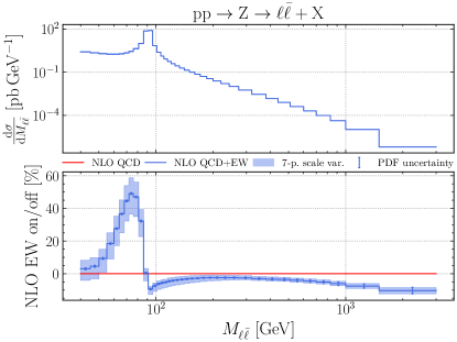
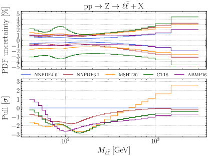
Figure 9.8: Same as Fig. 9.6 for $\mathrm{p}\mathrm{p}\to\ell\bar{\ell}+\mathrm{X}$.

For this process, mostly dominated by the exchange of an off-shell $\mathrm{Z}$, we require exactly two same-flavor opposite-sign leptons. These two leptons must satisfy the central acceptance cuts of $p_{\mathrm{T}}^{\ell}>15~{}{\rm GeV}$ and $|\eta_{\ell}|<2.4$, while their invariant mass must fulfill $40~{}{\rm GeV}<m_{\ell\bar{\ell}}<3000~{}{\rm GeV}$, similar to the CMS 13 TeV analysis [105]. The factorization and renormalization scales are set dynamically to $\mu=\langle m_{\ell\ell}\rangle$, where $\langle m_{\ell\ell}\rangle$ represents the center of each bin in the dilepton invariant mass distribution (see Fig. 9.8).

Charged vector-boson production.

This process is dominated by the exchange of an off-shell $\mathrm{W}$ boson, hence the acceptance cuts imposed on the final-state charged lepton (of any flavor) are $p_{\mathrm{T}}^{\ell}>20~{}{\rm GeV}$ and $|\eta_{\ell}|<2.5$. In this case we adopt fixed factorization and renormalization scales, set to the value of the $\mathrm{W}$-boson mass $\mu=m_{\mathrm{W}}$.

Diboson production.

We consider gauge boson pair production in the $\mathrm{Z}\mathrm{W}^{\pm}$ and $\mathrm{W}^{+}\mathrm{W}^{-}$ channels, with bosons subsequently decaying leptonically. We impose cuts on the final-state leptons of $p_{\mathrm{T}}^{\ell}>20~{}{\rm GeV}$ and $|\eta_{\ell}|<2.5$. In the $\mathrm{W}^{+}\mathrm{W}^{-}$ channel, we require two opposite-sign charged leptons from the boson decays with different lepton flavors. Also for this process we set $\mu=m_{\mathrm{W}}$.

Top pair production.

The simulation of this process is carried out at the level of stable top quarks. We impose that the invariant mass $m_{\mathrm{t}\bar{\mathrm{t}}}$ of the top-quark pair system be within the range $300~{}{\rm GeV}<m_{\mathrm{t}\bar{\mathrm{t}}}<2500~{}{\rm GeV}$, and adopt the same choice of binning as that used for CMS in their 13 TeV analysis [93] based on the lepton+jet final state. The factorization and renormalization scales depend on the event kinematics and are set dynamically to

$$\mu=H_{\mathrm{T}}/4={{1}\over{4}}\left[\sqrt{m_{\mathrm{t}}^{2}+(p_{\mathrm{T}}^{\mathrm{t}})^{2}}+\sqrt{m_{\mathrm{t}}^{2}+(p_{\mathrm{T}}^{\bar{\mathrm{t}}})^{2}}\right]\text{,}$$ (9.2)

where $p_{\mathrm{T}}^{\mathrm{t}}$ and $p_{\mathrm{T}}^{\bar{\mathrm{t}}}$ indicate the transverse momentum of the top and antitop quarks, respectively.

Higgs production via gluon fusion.

For the simulation of all the Higgs production processes we consider a stable Higgs, since its decays do not contain relevant information on the PDF sensitivity of the process. We require the Higgs to be produced in the central region, $|y_{\mathrm{H}}|<2.5$, and use fixed scales of $\mu=m_{\mathrm{W}}$.

Higgs production with associated $\mathrm{W}^{\pm}$ boson.

For this Higgs production channel, in addition to the central production requirement $|y_{\mathrm{H}}|<2.5$ we impose the same cuts on the charged lepton arising from the $\mathrm{W}^{\pm}$ decay as for charged-current Drell–Yan production, namely $p_{\mathrm{T}}^{\ell}>20~{}{\rm GeV}$ and $|\eta_{\ell}|<2.5$. Here we also set the scales to $\mu=m_{\mathrm{W}}$.

Higgs production in vector boson fusion.

In this case, in addition to the centrally produced Higgs we require a final state with (at least) two anti-$k_{\mathrm{t}}$ jets of radius $R=0.4$. These forward tagging jets must satisfy $p_{\mathrm{T}}^{\mathrm{j}}>20~{}{\rm GeV}$, $|y_{\mathrm{j}}|<4.5$, with a dijet invariant mass of $m_{\mathrm{j}_{1}\mathrm{j}_{2}}>500~{}{\rm GeV}$ and a rapidity separation of $|y_{\mathrm{j}_{1}}-y_{\mathrm{j}_{2}}|>2.5$, where $\mathrm{j}_{1}$ is the leading, and $\mathrm{j}_{2}$ the subleading jet (ordered in $p_{T}$). As for the other Higgs production processes, the scale is set to $\mu=M_{\mathrm{W}}$.

Results.

Using the calculational settings described above, we have computed differential distributions (to be discussed below) and then combined the bins into integrated cross-sections. Figs. 9.4 and 9.5 display the integrated LHC cross-sections at $14$ TeV for the processes under consideration: neutral and charged-current Drell–Yan production, gauge boson pair production, top-quark pair production, and Higgs production in different channels: gluon fusion, associated production with a $\mathrm{W}^{\pm}$ boson, and vector-boson fusion.

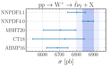
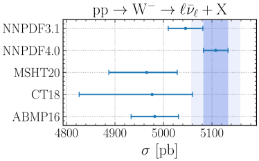
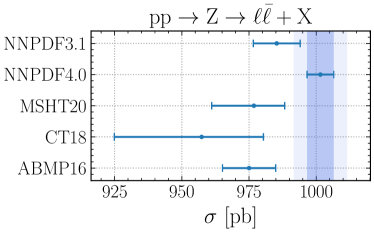
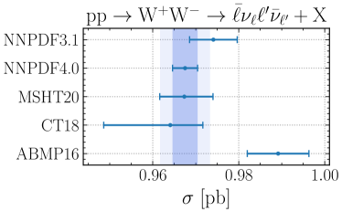
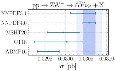
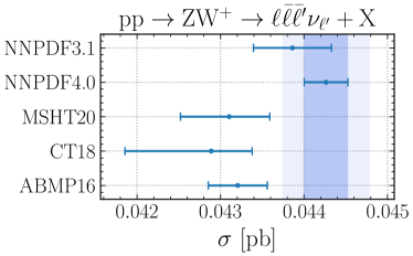
Figure 9.4: Integrated LHC cross-sections at $14$ TeV for neutral and charged-current Drell–Yan production (top) and gauge boson pair production (bottom) obtained with a variety of different PDF sets, all with $\alpha_{s}(m_{Z})=0.118$. The edges of $1\sigma$ and $2\sigma$ PDF uncertainty bands for NNPDF4.0 are indicated by dark and light lines respectively.

We compare results obtained using the NNPDF3.1, NNPDF4.0, CT18, MSHT20, and ABMP16 PDFs, in all cases with a common value of $\alpha_{s}(m_{Z})=0.118$. In order to facilitate visualization of the statistical compatibility between results obtained NNPDF4.0 and all other PDF sets, we display vertical bands indicating the $1\sigma$ (dark) and $2\sigma$ (light) uncertainty ranges of the NNPDF4.0 prediction. For CT18 and MSHT20, PDF uncertainties are computed with the asymmetric Hessian prescription so positive and negative uncertainties generally differ.

For charged- and neutral-current DY production, we observe good agreement at the $1\sigma$ level between NNPDF3.1 and NNPDF4.0, consistent with the comparisons at the luminosity level reported in Sect. 9.1. The NNPDF4.0 cross-sections are found to be higher than those of MSHT20 and CT18, as expected given the larger $\mathrm{q}\bar{\mathrm{q}}$ luminosity in the $m_{X}\simeq m_{V}$ region which dominates the integrated cross-section shown in Fig. 9.3, with central values in agreement at the $1\sigma$ or at most $2\sigma$ level. For these three cross-sections, the smaller PDF uncertainties of NNPDF4.0 compared to MSHT20 and especially CT18 that was observed in Sect. 9.1 is clearly visible.

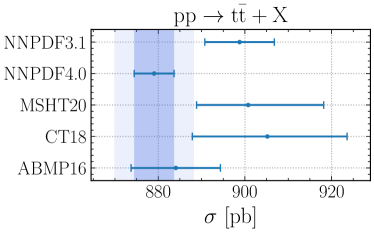
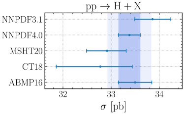
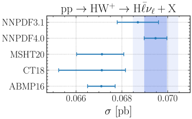
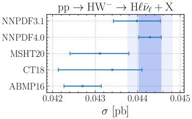
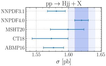
Figure 9.5: Same as Fig. 9.4 for top pair production and for Higgs production in different channels: gluon fusion, associated production with a $\mathrm{W}^{\pm}$ boson, and vector-boson fusion.

For the diboson production cross-sections, the comparison presents different features according to the specific final state. Indeed, diboson production is generally dominated by quark-quark scattering, so the specific partonic combination depends on the final state, and the total quark-quark luminosity $\mathcal{L}_{qq}$ only provides a crude average measure. While there is always excellent compatibility between NNPDF3.1 and NNPDF4.0, the comparison to other groups differs according to the specific process. For $\mathrm{W}^{+}\mathrm{W}^{-}$ production, NNPDF4.0 agrees well with CT18 and MSHT20, while the ABMP16 result is significantly larger. For $\mathrm{W}^{-}\mathrm{Z}$, NNPDF4.0 is somewhat higher than the other groups, though all except ABMP16 agree within uncertainties. For $\mathrm{W}^{+}\mathrm{Z}$ NNPDF4.0 is higher than the other groups by about $2\sigma$. NNPDF4.0 uncertainties are in general markedly smaller than those of the other groups, just as for DY production.

For top quark pair production, shown in Fig. 9.5, there is general agreement at the $1\sigma$ level, with NNPDF4.0 somewhat lower than CT18 and MSHT10, as expected from the luminosity comparison in the relevant invariant mass $m_{X}\simeq 450~{}{\rm GeV}$ region. Here too NNPDF4.0 leads to rather smaller PDF uncertainties.

For Higgs production we consider gluon fusion, associated production with vector bosons, and vector-boson fusion. For gluon fusion there is excellent agreement within uncertainties between all the groups. Interestingly, the NNPDF4.0 result, while still in excellent agreement with its NNPDF3.1 predecessor, now has a central value rather closer to that of the other groups. For associated production with gauge bosons, $\mathrm{H}\mathrm{W}^{+}$ and $\mathrm{H}\mathrm{W}^{-}$, the observed pattern is similar to charged-current DY, as expected due to the closely related underlying luminosities, with NNPDF3.1 and NNPDF4.0 in agreement and higher than other groups. For vector-boson-fusion, the NNPDF4.0 cross-section is higher than all the earlier determinations, and agrees best within uncertainties with MSHT20. In this case, NNPDF3.1 agreed better with other groups. Here too NNPDF4.0 uncertainties are the smallest.

9.3 Differential distributions

The integrated fiducial cross-sections discussed in the previous section are typically dominated by a localized region of the phase space corresponding to the bulk of the distribution, and hence they are only sensitive to PDFs in a narrow range of $x$ and $Q$. Differential distributions, that we now discuss, allow us to assess the compatibility between PDF sets also in regions where experimental constraints are scarce, such as the large $x$ region, relevant for searches of new massive particles, and the small-$x$ region, relevant for calculations of neutrino cross-sections for high-energy astrophysics [244].

For each differential distribution, we provide the absolute cross-sections obtained using NNPDF4.0, with theory uncertainties found by standard seven-point scale variation shown as a band. As mentioned, all computations are performed with NLO QCD accuracy: hence scale uncertainties would be smaller at NNLO. We then display the percentage shift between the pure QCD and the full QCD+EW computation, compared to the PDF and scale variation uncertainties. We next compare the relative PDF uncertainty found using all the PDF sets discussed in this Section. Finally we show the pull in units of the PDF uncertainty only between the result found using NNPDF4.0 and any of the other PDF sets, defined as

$$P\left(\sigma_{2,i},\sigma_{1,i}\right)\equiv{{\sigma^{(0)}_{2,i}-\sigma^{(0)}_{1,i}}\over{\sqrt{\left(\delta\sigma_{2,i}\right)^{2}+\left(\delta\sigma_{1,i}\right)^{2}}}}\,,\qquad i=1,\ldots,n_{\rm bin}\,,$$ (9.3)

where $\sigma^{(0)}_{1,i}$ and $\sigma^{(0)}_{2,i}$ are the central values of the theory predictions in the $i$-th bin and $\delta\sigma_{1,i}$, $\delta\sigma_{2,i}$ are the corresponding PDF uncertainties.

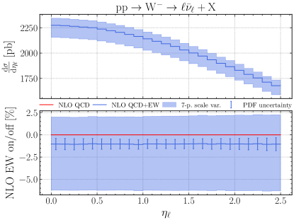
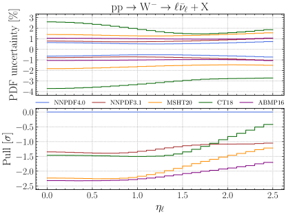
Figure 9.6: The differential distribution in charged lepton rapidity, $\eta_{\ell}$, for inclusive $l\bar{\nu}_{\ell}$ production. Note that the result of a fully off-shell calculation is presented; the heading in the plot indicates the dominant $W^{-}$ intermediate state. Predictions obtained using NNPDF3.1, NNPDF4.0, CT18, MSHT20, and ABMP16 are compared. We show the NNPDF4.0 absolute cross-sections (top left) with the band indicating the 7-point scale variation uncertainties; the percentage shift in central values between pure QCD and QCD+EW along with the PDF and scale variation uncertainties (bottom left), all for NNPDF4.0; the relative PDF uncertainties for all PDF sets (top right); and the pull defined in Eq. (9.3) between results obtained using NNPDF4.0 and each of the other PDF sets (bottom right).

We consider differential distributions for the following processes: charged current DY production (Figs. 9.6 and 9.7), neutral current DY (Fig. 9.12), gauge boson pair production (Figs. 9.9, 9.10, and 9.11), top pair production (Fig. 9.12), and then Higgs production in the various channels (Figs. 9.13, 9.14, 9.15, and 9.16). Recall that the fiducial cross-sections shown in the previous sections have been obtained by integrating the differential distributions shown here. Note also that in each case a fully off-shell calculation is presented, including nonfactorizable diagrams, and e.g. for diboson production also single and nonresonant contributions: so the heading in the diagram merely indicates the dominant intermediate state.

While detailed conclusions can be reached by inspection of the plots, we summarize here some generic features:

• PDF uncertainties are uniformly smallest for NNPDF4.0, and largest for CT18, with ABMP16 uncertainties sometimes close to the NNPDF4.0 ones. However, when comparing uncertainties in different PDF sets recall the caveat discussed in Sect. 9.1.

• The pull is essentially always below one for NNPDF3.1, thus showing backward compatibility of NNPDF4.0 with its predecessor.

• The pull is generally largest for ABMP16, especially in regions sensitive to extrapolation where the uncertainties are very small for this PDF set, such as for instance highly boosted associate Higgs production with $W^{\pm}$, where in the largest rapidity bins the pull can be as large as four.

• The pulls of CT18 and MSHT20 for the more inclusive observables, single gauge boson production and Higgs in gluon fusion, are generally below two and mostly below one. However, pulls for double gauge-boson production and associate Higgs production or Higgs in gauge fusion are larger and sometimes exceed two.

• Large pulls with CT18 and MSHT20 are also seen for top production at large invariant mass, where the gluon at increasingly large $x$ is probed, in agreement with the comparison of gluon luminosities.

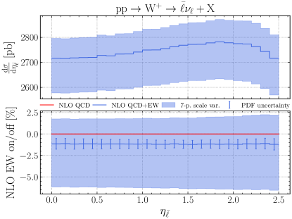
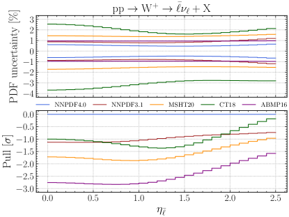
Figure 9.7: Same as Fig. 9.6 for $\mathrm{p}\mathrm{p}\to\bar{\ell}\nu_{\ell}+\mathrm{X}$.

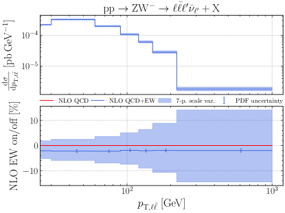
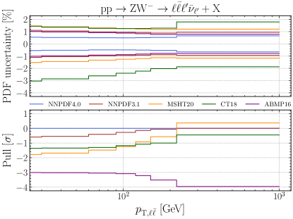
Figure 9.9: Same as Fig. 9.6 for $\mathrm{p}\mathrm{p}\to\ell\bar{\ell}\ell^{\prime}\bar{\nu}_{\ell^{\prime}}+\mathrm{X}$.

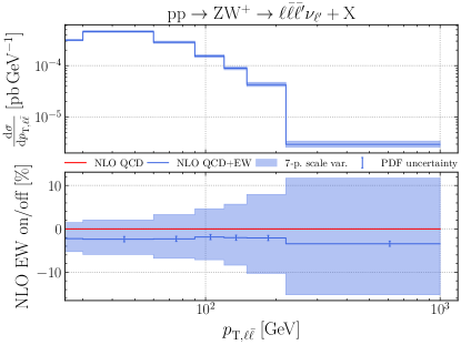
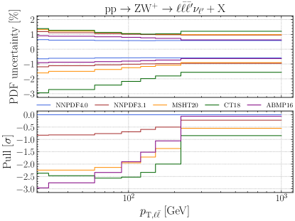
Figure 9.10: Same as Fig. 9.6 for $\mathrm{p}\mathrm{p}\to\ell\bar{\ell}\bar{\ell}^{\prime}\nu_{\ell^{\prime}}+\mathrm{X}$.

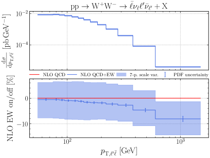
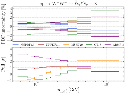
Figure 9.11: Same as Fig. 9.6 for $\mathrm{p}\mathrm{p}\to\bar{\ell}\nu_{\ell}\ell^{\prime}\bar{\nu}_{\ell^{\prime}}+\mathrm{X}$.

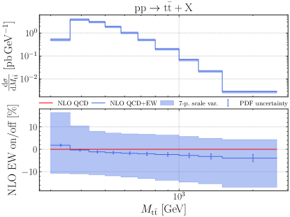
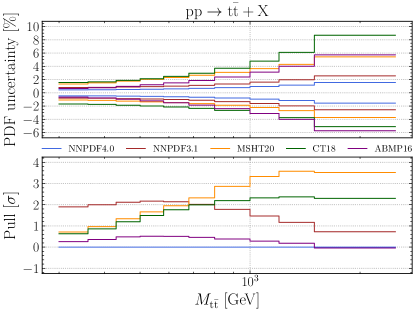
Figure 9.12: Same as Fig. 9.6 for $\mathrm{p}\mathrm{p}\to\mathrm{t}\bar{\mathrm{t}}+\mathrm{X}$.

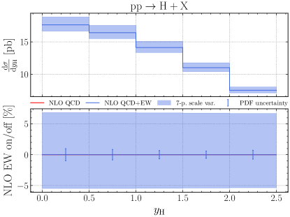
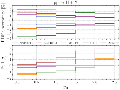
Figure 9.13: Same as Fig. 9.6 for $\mathrm{p}\mathrm{p}\to\mathrm{H}+\mathrm{X}$.

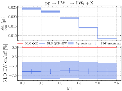
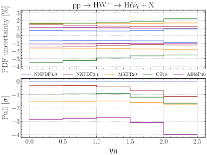
Figure 9.14: Same as Fig. 9.6 for $\mathrm{p}\mathrm{p}\to\mathrm{H}\ell\bar{\nu}_{\ell}+\mathrm{X}$.

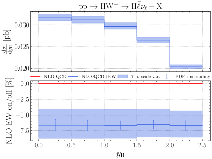
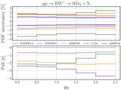
Figure 9.15: Same as Fig. 9.6 for $\mathrm{p}\mathrm{p}\to\mathrm{H}\bar{\ell}\nu_{\ell}+\mathrm{X}$.

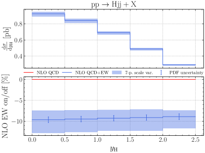
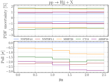
Figure 9.16: Same as Fig. 9.6 for $\mathrm{p}\mathrm{p}\to\mathrm{H}\mathrm{j}\mathrm{j}+\mathrm{X}$.

10 Deliverables, summary and outlook

The NNPDF4.0 PDF set presented in this paper consists of two main classes of deliverables. The first class includes, as customary, the public release of various PDF sets, delivered in standard LHAPDF6 interpolation grid format [32]. The other class is, for the first time, the release of the complete NNPDF fitting framework as an open-source code, including extensive documentation and user-ready examples. The availability of the NNPDF code as open source guarantees the complete reproducibility of any aspect of the PDF determination presented in this work: construction and hyperoptimization of the methodology, computation of observables, PDF determination, statistical validation of results, and visualization through suitable tools. We believe that the full open-source availability of our PDF fitting framework represents a significant contribution to the LHC and QCD research communities, as well as a major step towards the achievement of the FAIR (findability, accessibility, interoperability, and reusability) principles [245]. As such, our code and data should be fully and freely reusable by both humans and machines.

The publicly available open-source NNPDF code is briefly described in Appendix A and more extensively in a dedicated companion paper [31]. Below we list the NNPDF4.0 PDF sets that we are making available. We then provide a summary and outlook of this work.

10.1 PDF grids

The NNPDF4.0 PDF sets are made publicly available via the LHAPDF6 interface,

http://lhapdf.hepforge.org/  .

All sets are delivered as sets of $N_{\rm rep}=100$ Monte Carlo replicas. In the case of the baseline NNLO, the 100-replica set is obtained from compression of a larger $N_{\rm rep}=1000$ replica set, which is also made available, and a Hessian conversion with $N_{\rm eig}=50$ eigenvectors of the 1000-replica set is also made available. We have checked that the 50 eigenvector set guarantees an accuracy comparable to that of the PDF4LHC combined set [237, 215], namely at or better than the 10-20% level on correlations and at the percent level on uncertainties.

• Baseline LO, NLO and NNLO NNPDF4.0 sets.

  The baseline LO, NLO, and NNLO NNPDF4.0 sets are based on the global dataset, with $\alpha_{s}(m_{Z})=0.118$ and a variable-flavor-number scheme with up to five active flavors. These sets contain $N_{\rm rep}=100$ replicas each and their file grid names are

  NNPDF40_lo_as_01180
  NNPDF40_nlo_as_01180
  NNPDF40_nnlo_as_01180

  The NNLO set has been obtained from the optimized compression [28, 29] of a dedicated $N_{\rm rep}=1000$ replica set, which is also made also available

  NNPDF40_nnlo_as_01180_1000

  and whose usage is recommended for applications that require a large replica sample, such as Bayesian reweighting [155, 156]. This $N_{\rm rep}=1000$ replica set is also used as input for the Hessian conversion [26, 27], producing a set with $N_{\rm rep}=50$ eigenvectors with grid name

  NNPDF40_nnlo_as_01180_hessian

• PDF sets with $\alpha_{s}$ variations.

  NNLO PDF sets with baseline theory settings are made available for a variety of values of the strong coupling spanning a range of $\alpha_{s}(m_{Z})$ from 0.116 to 0.120:

  NNPDF40_nnlo_as_01160
  NNPDF40_nnlo_as_01170
  NNPDF40_nnlo_as_01175
  NNPDF40_nnlo_as_01185
  NNPDF40_nnlo_as_01190
  NNPDF40_nnlo_as_01200
  

  Also, two NLO sets with $\alpha_{s}$ varied by $\pm 0.001$ about the central value are provided:

  NNPDF40_nlo_as_01170
  NNPDF40_nlo_as_01190
  

  In order to facilitate the computation of combined PDF+$\alpha_{s}$ uncertainties, we provide bundled PDF+$\alpha_{s}$ variation sets for $\alpha_{s}(m_{Z})=0.118\pm 0.001$ both for the NNLO Monte Carlo and Hessian baseline sets:

  NNPDF40_nnlo_pdfas
  NNPDF40_nnlo_hessian_pdfas
  

  These bundled PDF sets have been constructed as follows: for the Monte Carlo sets

  1. The central value (PDF member 0) is the central value of the corresponding $\alpha_{s}(m_{Z})=0.118$ set;

  2. PDF members 1 to 100 correspond to the $N_{\mathrm{rep}}=100$ Monte Carlo replicas;

  3. the PDF members 101 and 102 are the central values of the sets with $\alpha_{s}(m_{Z})=0.117$ and $\alpha_{s}(m_{Z})=0.119$ respectively;

  while for the Hessian sets

  1. The central value (PDF member 0) is the central value of the corresponding $\alpha_{s}(m_{Z})=0.118$ set;

  2. members from 1 to 50 correspond to the $N_{\rm eig}=50$ eigenvectors from the $\alpha_{s}(m_{Z})=0.118$ set;

  3. members 51 and 52 are the central values of the sets with $\alpha_{s}(m_{Z})=0.117$ and $\alpha_{s}(m_{Z})=0.119$ respectively.

  The usage of these bundled sets to evaluate the combined PDF+$\alpha_{s}$ uncertainties for LHC cross-sections is explained e.g. in [237].

• PDF sets with perturbative charm.

  In the NNPDF4.0 baseline the charm PDF is independently parametrized, along with light quark PDFs. Variants in which charm is not independently parametrized, but rather obtained from perturbative matching conditions and the FONLL scheme is used, are also made available. We release LO, NLO, and NNLO Monte Carlo sets with $N_{\rm rep}=100$ PDF replicas each:

  NNPDF40_lo_pch_as_01180
  NNPDF40_nlo_pch_as_01180
  NNPDF40_nnlo_pch_as_01180

• PDF sets with flavor-number variations.

  The baseline NNPDF4.0 PDFs are based on a variable-flavor-number scheme with a maximum of $n_{f}=5$ active flavors. We have also produced sets, both at NLO and NNLO, in which the maximum value of $n_{f}$ is either 4 or 6

  NNPDF40_nlo_as_01180_nf_4
  NNPDF40_nlo_as_01180_nf_6
  NNPDF40_nnlo_as_01180_nf_4
  NNPDF40_nnlo_as_01180_nf_6
  

  as well as variants of the perturbative charm fit in the $n_{f}=3$ scheme

  NNPDF40_nlo_pch_as_01180_nf_3
  NNPDF40_nnlo_pch_as_01180_nf_3
  

  Note that these grids are constructed by taking the baseline PDF sets as a fixed boundary condition and then adjusting the settings of perturbative evolution and the running of $\alpha_{s}$ to the desired $n_{f}$ scheme. For instance, the NNPDF40_nnlo_as_0118_nf_4 is identical to the baseline NNPDF40_nnlo_as_0118 for $Q\leq m_{b}$ but differs from it for $Q>m_{b}$ due to the different number of active flavors in the evolution of $\alpha_{s}(Q)$ and PDFs.

  It is important to observe that, consequently, the value of the strong coupling in the $n_{f}=3$ and $n_{f}=4$ schemes is modified and it is $\alpha_{s}(m_{Z})\neq 0.118$. The naming convention adopted is that the value of $\alpha_{s}(m_{Z})$ used is that corresponding to $\alpha_{s}(m_{Z})=0.118$ in the $n_{f}=5$ flavor scheme.

  In the $n_{f}=4$ case, bundled sets with $\alpha_{s}$ variations are also constructed following the same strategy as in the baseline fits

  NNPDF40_nlo_nf_4_pdfas
  NNPDF40_nnlo_nf_4_pdfas
  

• PDF sets with dataset variations.

  The variants of NNPDF4.0 with different input datasets, in particular those discussed in Sect. 7, are made available in the LHAPDF6 format and have been linked to the NNPDF website:

  https://nnpdf.mi.infn.it/nnpdf4-0/

  Note that these consist of fits based both on subsets of the baseline dataset, such as the collider-only PDFs, as well as fits where additional datasets have been included, such as the those with the NOMAD or the HERA jet cross-sections.

In addition to the grid files explicitly listed here, the rest of the PDF sets discussed in this paper are also available upon request. We also emphasize that since the fitting code is made public, see Appendix A, arbitrary variants of the present NNPDF4.0 determination can be produced by interested users.

10.2 Summary and outlook

The NNPDF4.0 set presented here is characterized by the feature of exhibiting a remarkable precision, with PDF uncertainties of order of 1% in a wide kinematic region for several PDF combinations. This is mostly a consequence of having used in its determination a machine learned methodology, that combines a significantly more general and flexible parametrization with a very efficient minimization.

The general features of the underlying dataset support the reliability of these small uncertainties. Specifically, the determination is now dominated by collider data, which are generally more reliable than older fixed-target data: indeed, DIS-only and no-LHC PDFs now differ substantially from the global fit, and HERA data are no longer needed in order to fix the small-$x$ behavior of PDFs. Furthermore, there is generally good or excellent compatibility between all the disparate pieces of information that enter the global PDF determination, also thanks to the dataset selection procedure that has been applied, as discussed in Sect. 4, with most of all data leading to mutually consistent constraints on PDF. This is supported by the inspection of alternative PDF determinations in which individual data or sets of data are removed, see Sect. 7. Finally, the PDF fit includes many datasets that provide mutually consistent constraints on the same PDF. For instance, the $\bar{d}/\bar{u}$ ratio, that is in principle constrained by the SeaQuest data, is actually predicted with almost unchanged precision by a fit in which this data are not used, and the same is true for the charm PDF and the EMC structure function data, or for strangeness and the NOMAD neutrino DIS data, or for the gluon and HERA DIS jet data.

The excellent control on the individual PDF flavors achieved in the NNPDF4.0 determination suggests that it would be interesting to carry out a detailed assessment of the non-perturbative structure of the proton, specifically by comparing to models of proton structure and lattice QCD calculations for quantities such as the $\bar{d}/\bar{u}$ and $d/u$ ratios in the large $x$ region, the strangeness content, and intrinsic charm. This analysis will be presented in a dedicated publication [233].

In terms of methodology, the reliability of results for PDF uncertainties is backed up by extensive closure testing and future testing, see Sect. 6, and by the stability upon the methodological variations considered in Sect. 8, specifically the lack of dependence on the choice of fitting basis, which is a highly nontrivial check that we performed here for the first time.

However, it is clear that percent-level PDF uncertainties must be treated with caution, and in particular it is important to consider carefully sources of uncertainty that might have been underestimated, or that have not been included.

The first and most obvious one is missing higher order uncertainties, routinely estimated by scale variation, that are not included in PDF uncertainties. Their inclusion is possible using the methodology developed in Refs. [23, 24, 246]. The inclusion of uncertainties related to missing higher perturbative orders in QCD calculations will be crucial in ensuring full reliability of central values and uncertainties to percent or sub-percent accuracy. A closely related aspect which deserves direct investigation is the construction of PDF sets at N³LO in QCD, which is already possible by using suitable approximations, specifically for anomalous dimensions [247]. These will be useful both directly, for consistency with LHC calculations where matrix elements are evaluated at the same perturbative order, and as a means to accurately estimate uncertainties on NNLO results.

Also, NNLO QCD corrections at present are largely included through $K$-factors. Their full analytic inclusion should be soon possible, as fully differential Monte Carlo generators accurate to NNLO QCD [248, 249, 123] and fast-interpolation grids supporting NNLO QCD corrections [128, 129, 130, 16] become more widely available.

Furthermore, at present the impact of electroweak corrections is only verified a posteriori. Rather, they should be included systematically in theory predictions, alongside with a photon PDF. The construction of a QED variant of NNPDF4.0 including coupled QED$\otimes$QCD evolution, along the lines of its NNPDF3.1QED predecessor [202], will be an immediate task, but a full PDF determination in which mixed QCD-EW corrections are fully included up to NLO will be needed for full theoretical reliability. Such a determination should also include an estimate of the missing higher order electroweak corrections.

Finally, the machine-learning methodology that we have followed is based on standard traditional $\chi^{2}$ minimization, and it has been closure-tested to fully consistent pseudodata. This might miss information contained in the full statistical features of the PDF fit, of which the $\chi^{2}$ is only the simplest indicator, and specifically it might lead to uncertainty estimation in the presence of incompatible data and inaccuracies in the estimation of experimental uncertainties. It should be improved through the exploration and use of a more advanced methodology, both for PDF determination and for validation (including closure testing) in which the full statistical features of the dataset and the ensuing PDFs are used.

All these developments are the focus of ongoing studies, with the goal of achieving PDFs with fully reliable sub-percent accuracy.

 

Acknowledgements

We thank Amanda Cooper-Sarkar, Thomas Cridge, Lucian Harland-Lang, Timothy Hobbs, Joey Houston, Pavel Nadolsky, Gavin Salam and Robert Thorne for discussions. We thank Andrew Pilkington and Reinhard Schwienhorst for help with the ATLAS measurements; Maria Aldaya, Emanuela Barberis and Alberto Orso Maria Iorio for assistance with the CMS data; and Stephen Farry and Oliver Lupton for help with the LHCb data. We are grateful to Jun Gao for providing us with the NNLO $K$-factors for the NuTeV, NOMAD, and ATLAS and CMS single-top measurements, and for helping us with the benchmark of the corresponding NLO calculations. We are grateful to Daniel Britzger for providing us with NNLO fast interpolation grids for the HERA jet data and to Thomas Gehrmann, Aude Gehrmann-De Ridder, Nigel Glover, Alexander Huss and Joao Pires for providing us with NNLO $K$-factors for ATLAS and CMS jet measurements. We thank Valerio Bertone for assistance with the correction of a bug in APFEL, Marco Zaro for support with MadGraph5_aMC@NLO and Luca Rottoli for guidance in the computation of NNLO corrections for fixed-target Drell–Yan measurements on deuteron targets. We acknowledge contributions from Rabah Abdul Khalek, Alessandro Candido, Felix Hekhorn, Giacomo Magni, Tanjona Rabemananjara and Giovanni Stagnitto at various stages of this work.

S. C., S. F., J. C.-M., R. S and C. S. are supported by the European Research Council under the European Union’s Horizon 2020 research and innovation Programme (grant agreement n.740006). M. U. and Z. K. are supported by the European Research Council under the European Union’s Horizon 2020 research and innovation Programme (grant agreement n.950246). M. U. and S. I. are supported by the Royal Society grant RGF/EA/180148. The work of M. U. is also funded by the Royal Society grant DH150088. The work of M. U., S. I., C. V. and Z. K. is partially supported by the STFC consolidated grant ST/L000385/1. The work of Z.K. was partly supported by supported by the European Research Council Consolidator Grant “NNLOforLHC2”. The work of ZK was previously supported by the European Commission grant (683211) R. D. B, L. D. D. and E. R. N. are supported by the U.K. Science and Technology Facility Council (STFC) grant ST/P000630/1. E. R. N. was also supported by the European Commission through the Marie Skłodowska-Curie Action ParDHonS (grant number 752748). J. R. is partially supported by NWO, the Dutch Research Council. T. G. is supported by The Scottish Funding Council, grant H14027, R. L. P. and M. W. by the STFC grant ST/R504737/1 and C. V by the STFC grant ST/R504671/1.

Appendix A The open-source NNPDF code

The open-source NNPDF code is the subject of a separate dedicated publication [31], to which the reader is referred for details, while here we provide a brief summary. The NNPDF fitting framework consists of an extensive array of tools for global analysis of non-perturbative QCD quantities. While the current version of the code focuses on unpolarized parton distributions, its flexible infrastructure is extensible to many other related objects such as polarized PDFs, nuclear PDFs, or fragmentation functions.

The NNPDF code is available from its GitHub repository

https://github.com/NNPDF/nnpdf

and is fully documented in

https://docs.nnpdf.science/

The main inputs of the NNPDF code are the experimental data, stored in a common format, and the theoretical calculations. The latter are provided in the form of fast grids such as APPLgrid [127], FastNLO [130], or PineAPPL [16], which are then combined [118] with QCD evolution kernels to produce FK interpolation tables [199, 189] and possibly supplemented with NNLO QCD and/or NLO electroweak $K$-factors. The user needs also to provide the settings and parameters of the theory calculations, such as the value of $\alpha_{s}(m_{Z})$, the heavy quark masses and the perturbative order.

All the settings that determine the outcome of a given PDF determination, from input datasets to theory settings and the parameters of the optimizer, can be adjusted in the corresponding run card written in YAML. This runcard is the unique identifier of a determination and contains all required information to perform (and reproduce) a global PDF fit. Instructions on how to set up a runcard and use it to launch a fit can be found in

https://docs.nnpdf.science/tutorials/run-fit.html

and examples of runcards used to produce the PDF sets presented in this paper are collected in

https://github.com/NNPDF/nnpdf/tree/master/n3fit/runcards/reproduce_nnpdf40

For instance, via the runcard the user can select the neural network architecture or the specific variant of the SGD optimizer. They can also define the ranges of hyperparameters and determine automatically the optimal values by means of the hyperopt method described in Sect. 3.3.

The NNPDF code is composed of the following main packages:

The buildmaster experimental data formatter

A C++ program that transforms the experimental data as originally provided by HepData into a common standard format tailored for PDF fitting, for instance by allowing different treatments of the correlated systematic uncertainties.

The APFELcomb interpolation table generator

A code that takes as input fast NLO interpolation grids and combines them with the evolution kernels provided by APFEL to produce FK tables, which map the PDFs at the input parametrization scale $Q_{0}$ to physical observables.

The n3fit fitting code

A TensorFlow-based code which carries out the training of neural networks by means of a variety of SGD algorithms. The hyperparameters that determine the outcome of the training can either be selected by hand or determined automatically by means of the hyperopt procedure. The flexibility and modularity of n3fit ensures that, should that be required, the user can interface the code with new optimization algorithms of their choice.

The validphys analysis framework

Implemented in reportengine [250], this code collects the outcome of a PDF fit and produces a complete HTML training report with all relevant information such as plots of the PDFs, parton luminosities and physical observables and statistical estimators from the $\chi^{2}$ to the arc-length. The extensive functionalities of this framework are described in

https://docs.nnpdf.science/vp/index.html

All the plots and tables presented in this paper have been obtained using this validphys framework, which also provides tools to interact with online resources such as the results of previous fits or precomputed sets of FK tables, which are automatically downloaded when required by a runcard.

The libnnpdf C++ fitting code

This is the code underlying the NNPDF3 family of PDF determinations, and provides backwards compatibility such that users can reproduce the outcome of NNPDF3.1-like global fits.

These various components of the NNPDF fitting code are available as binary packages accessible through conda. This allows for a smooth installation alongside with that of all relevant dependencies and external packages. Crucially, one can indicate specific versions of both the fitting code and of its dependencies, ensuring the full reproducibility of the result of a given PDF fit.

As discussed in [31], as with any open-source code we welcome suggestions and requests for improvements and addition of new features. For instance, a new feature can be requested by either creating an issue in the GitHub repository or by means of a pull request. The latter would undergo review, testing, and validation before being eventually approved and merged into the master code.

Appendix B Input datasets in PDF fits

In order to put the NNPDF4.0 PDF determination in context, we provide here tables comparing the NNPDF4.0 dataset to that adopted for the other PDF determinations considered in the main body of the paper, namely NNPDF3.1 [5], ABMP16 [142], CT18 [143] and MSHT20 [144].

Tables B.1–B.6 collect all the data used for the construction of these PDF sets. For each dataset, we provide the corresponding reference and indicate with a blue tick or a red cross whether or not this dataset is part of each PDF analysis. A parenthesized tick in a yellow box denotes that a dataset was investigated, but for various reasons not included in the baseline fit:

• for NNPDF3.1 these are the datasets given in tables 2.1 and 2.3 of Ref. [5], which are marked with square brackets,

• similarly for NNPDF4.0, where the datasets are given in Tab. 2.1, 2.4 and 2.5, also marked with square brackets,

• for ABMP16 they are mentioned in the text in section II.A of Ref. [142],

• for CT18 the datasets are discussed in section II.A.2 and II.B.6 of Ref. [143]

• and finally for MSHT20 the datasets are given in section 10 of Ref. [144].

Data set	Ref.	NNPDF3.1	NNPDF4.0	ABMP16	CT18	MSHT20
NMC $F_{2}^{d}/F_{2}^{p}$	[33]	✓	✓	✗	✗	✓
NMC $\sigma^{{\rm NC},p}$	[34]	✓	✓	✗	✓	✓
SLAC $F_{2}^{p},F_{2}^{d}$	[251, 35]	✓	✓	✓	✗	✓
BCDMS $F_{2}^{p}$	[36]	✓	✓	✓	✓	✓
BCDMS $F_{2}^{d}$	[252]	✓	✓	✗	✓	✓
BCDMS, NMC, SLAC $F_{\mathrm{L}}$	[36, 34, 251]	✗	✗	✗	✗	✓
CHORUS $\sigma_{CC}^{\nu},\sigma_{CC}^{\bar{\nu}}$	[37]	✓	✓	✗	✗	✓
CHORUS	[253]	✗	✗	✓	✗	✗
NuTeV $F_{2},F_{3}$	[254]	✗	✗	✗	✗	✓
NuTeV/CCFR $\sigma_{CC}^{\nu},\sigma_{CC}^{\bar{\nu}}$	[38]	✓	✓	✓	✓	✓
EMC $F_{2}^{c}$	[44]	(✓)	(✓)	✗	✗	✗
NOMAD	[111]	✗	(✓)	✓	✗	✗
CCFR $xF_{3}^{p}$	[255]	✗	✗	✗	✓	✗
CCFR $F_{2}^{p}$	[256]	✗	✗	✗	✓	✗
CDSHW $F_{2}^{p},xF_{3}^{p}$	[257]	✗	✗	✗	✓	✗
E665 $F_{2}^{p},F_{2}^{d}$	[258]	✗	✗	✗	✗	✓
HERA NC, CC	[259]	✗	✗	✗	✗	✓
HERA I+II $\sigma^{p}_{\rm NC,CC}$	[40]	✓	✓	✓	✓	✗
HERA I+II $\sigma_{c\bar{c}}^{\rm red}$	[145]	✗	✓	✗	(✓)	✓
HERA I+II $\sigma_{b\bar{b}}^{\rm red}$	[145]	✗	✓	✗	(✓)	✗
HERA I+II $\sigma_{c\bar{c}}^{\rm red}$	[41]	✓	✗	✓	✓	✗
H1 $F_{2}^{c\bar{c}}$	[260]	✗	✗	✗	✓	✗
H1 $F_{2}^{b\bar{b}}$	[42]	✓	✗	✓	✗	✗
ZEUS $\sigma_{b\bar{b}}^{\mathrm{red}}$	[43]	✓	✗	✓	✗	✗
H1 $F_{\mathrm{L}}$	[261]	✗	✗	✗	✓	✓
H1 and ZEUS $F_{\mathrm{L}}$	[262, 263]	✗	✗	✗	✗	✓
ZEUS 820 (HQ) (1j)	[112]	✗	(✓)	✗	✗	✗
ZEUS 920 (HQ) (1j)	[113]	✗	(✓)	✗	✗	✗
H1 (LQ) (1j-2j)	[115]	✗	(✓)	✗	✗	✗
H1 (HQ) (1j-2j)	[116]	✗	(✓)	✗	✗	✗
ZEUS 920 (HQ) (2j)	[114]	✗	(✓)	✗	✗	✗

Table B.1: The fixed-target and collider DIS measurements used for PDF determination. For each PDF set, a blue tick indicates that the given dataset is included and a red cross that it is not included. A parenthesized tick denotes that a dataset was investigated but not included in the baseline fit.

Data set	Ref.	NNPDF3.1	NNPDF4.0	ABMP16	CT18	MSHT20
DY E866 $\sigma^{d}_{\rm DY}/\sigma^{p}_{\rm DY}$ (NuSea)	[47]	✓	✓	✓	✓	✓
DY E866 $\sigma^{p}_{\rm DY}$	[46]	✓	✓	✗	✓	✓
DY E605 $\sigma^{p}_{\rm DY}$	[45]	✓	✓	✓	✓	✗
DY E906 $\sigma^{d}_{\rm DY}/\sigma^{p}_{\rm DY}$ (SeaQuest)	[117]	✗	✓	✗	✗	✗

Table B.2: Same as Table B.1 for fixed-target Drell–Yan data sets.

Data set	Ref.	NNPDF3.1	NNPDF4.0	ABMP16	CT18	MSHT20
CDF $Z$ rapidity	[48]	✓	✓	✗	✓	✓
CDF $W\to\ell\nu$ asymmetry ($1.8$ TeV)	[264]	✗	✗	✗	✓	✗
CDF $W\to e\nu$ asymmetry ($\mathcal{L}=170$ pb-1)	[265]	✗	✗	✗	✓	✗
CDF $W\to e\nu$ asymmetry ($\mathcal{L}=1$ fb-1)	[266]	✗	✗	✗	✗	✓
CDF $k_{t}$ inclusive jets	[52]	✓	✗	✗	✗	✓
CDF cone-based inclusive jets	[267]	✗	✗	✗	✓	✗
D0 $Z$ rapidity	[49]	✓	✓	✗	✓	✓
D0 $W\to e\nu$ asymmetry ($\mathcal{L}=0.75$ fb-1)	[268]	✗	✗	✗	✗	✓
D0 $W\to e\nu$ (prod.) asymmetry ($\mathcal{L}=9.7$ fb-1)	[269]	✗	✗	(✓)	✗	✓
D0 $W\to e\nu$ (prod. and decay) asymmetry ($\mathcal{L}=9.7$ fb-1)	[51]	✓	(✓)	✓	✓	✗
D0 $W\to\mu\nu$ asymmetry ($\mathcal{L}=0.3$ fb-1)	[270]	✗	✗	✗	✓	✗
D0 $W\to\mu\nu$ asymmetry ($\mathcal{L}=7.3$ fb-1)	[50]	✓	✓	✓	✗	✓
D0 cone-based inclusive jets	[271]	✗	✗	✗	✓	✓
CDF and D0 top-pair production	[272]	✗	✗	(✓)	✗	✓
CDF and D0 single-top production	[273]	✗	✗	✓	✗	✗

Table B.3: Same as Table B.1 for Tevatron data sets.

Data set	Ref.	NNPDF3.1	NNPDF4.0	ABMP16	CT18	MSHT20
ATLAS $W,Z$ 7 TeV ($\mathcal{L}=35$ pb-1)	[53]	✓	✓	✓	✓	✓
ATLAS $W,Z$ 7 TeV ($\mathcal{L}=4.6$ fb-1)	[54]	✓	✓	✗	(✓)	✓
ATLAS low-mass DY 7 TeV	[55]	✓	✓	✗	(✓)	✗
ATLAS high-mass DY 7 TeV	[56]	✓	✓	✗	(✓)	✓
ATLAS $W$ 8 TeV	[81]	✗	(✓)	✗	✗	✓
ATLAS DY 2D 8 TeV	[80]	✗	✓	✗	✗	✓
ATLAS high-mass DY 2D 8 TeV	[79]	✗	✓	✗	(✓)	✓
ATLAS $\sigma_{W,Z}$ 13 TeV	[83]	✗	✓	✓	✗	✗
ATLAS $W$+jet 8 TeV	[95]	✗	✓	✗	✗	✓
ATLAS $Z$ $p_{T}$ 7 TeV	[274]	(✓)	✗	✗	(✓)	✗
ATLAS $Z$ $p_{T}$ 8 TeV	[65]	✓	✓	✗	✓	✓
ATLAS $W+c$ 7 TeV	[85]	✗	✓	✗	(✓)	✗
ATLAS $\sigma_{tt}^{\rm tot}$ 7, 8 TeV	[67]	✓	✓	✓	✗	✗
ATLAS $\sigma_{tt}^{\rm tot}$ 7, 8 TeV	[275, 276, 277, 278, 279, 280]	✗	✗	✓	✗	✗
ATLAS $\sigma_{tt}^{\rm tot}$ 13 TeV ($\mathcal{L}=3.2$ fb-1)	[68]	✓	✗	✓	✗	✗
ATLAS $\sigma_{tt}^{\rm tot}$ 13 TeV ($\mathcal{L}=139$ fb-1)	[136]	✗	✓	✗	✗	✗
ATLAS $\sigma_{tt}^{\rm tot}$ and $Z$ ratios	[281]	✗	✗	✗	✗	(✓)
ATLAS $t\bar{t}$ lepton+jets 8 TeV	[69]	✓	✓	✗	✓	✓
ATLAS $t\bar{t}$ dilepton 8 TeV	[91]	✗	✓	✗	✗	✓
ATLAS single-inclusive jets 7 TeV, R=0.6	[75]	✓	(✓)	✗	✓	✓
ATLAS single-inclusive jets 8 TeV, R=0.6	[88]	✗	✓	✗	✗	✗
ATLAS dijets 7 TeV, R=0.6	[148]	✗	✓	✗	✗	✗
ATLAS direct photon production 8 TeV	[102]	✗	(✓)	✗	✗	✗
ATLAS direct photon production 13 TeV	[103]	✗	✓	✗	✗	✗
ATLAS single top $R_{t}$ 7, 8, 13 TeV	[96, 100, 98]	✗	✓	✓	✗	✗
ATLAS single top diff. 7 TeV	[96]	✗	✓	✗	✗	✗
ATLAS single top diff. 8 TeV	[98]	✗	✓	✗	✗	✗

Table B.4: Same as Table B.1 for ATLAS data sets.

Data set	Ref.	NNPDF3.1	NNPDF4.0	ABMP16	CT18	MSHT20
CMS $W$ asym. 7 TeV ($\mathcal{L}=36$ pb-1)	[282]	✗	✗	✗	✗	✓
CMS $Z$ 7 TeV ($\mathcal{L}=36$ pb-1)	[283]	✗	✗	✗	✗	✓
CMS $W$ electron asymmetry 7 TeV	[57]	✓	✓	✗	✓	✓
CMS $W$ muon asymmetry 7 TeV	[58]	✓	✓	✓	✓	✗
CMS Drell-Yan 2D 7 TeV	[59]	✓	✓	✗	(✓)	✓
CMS Drell-Yan 2D 8 TeV	[284]	(✓)	✗	✗	✗	✗
CMS $W$ rapidity 8 TeV	[60]	✓	✓	✓	✓	✓
CMS $W,Z$ $p_{T}$ 8 TeV ($\mathcal{L}=18.4$ fb-1)	[285]	✗	✗	✗	(✓)	✗
CMS $Z$ $p_{T}$ 8 TeV	[66]	✓	✓	✗	(✓)	✗
CMS $W+c$ 7 TeV	[78]	✓	✓	✗	(✓)	✓
CMS $W+c$ 13 TeV	[86]	✗	✓	✗	✗	(✓)
CMS single-inclusive jets 2.76 TeV	[77]	✓	✗	✗	✗	✓
CMS single-inclusive jets 7 TeV	[147]	✓	(✓)	✗	✓	✓
CMS dijets 7 TeV	[76]	✗	✓	✗	✗	✗
CMS single-inclusive jets 8 TeV	[89]	✗	✓	✗	✓	✓
CMS 3D dijets 8 TeV	[149]	✗	(✓)	✗	✗	✗
CMS $\sigma_{tt}^{\rm tot}$ 5 TeV	[90]	✗	✓	✗	✗	✗
CMS $\sigma_{tt}^{\rm tot}$ 7, 8 TeV	[146]	✓	✓	✗	✗	✗
CMS $\sigma_{tt}^{\rm tot}$ 8 TeV	[286]	✗	✗	✗	✗	✓
CMS $\sigma_{tt}^{\rm tot}$ 5, 7, 8, 13 TeV	[70, 287, 288, 289, 290, 291, 292, 293, 294, 295]	✗	✗	✓	✗	✗
CMS $\sigma_{tt}^{\rm tot}$ 13 TeV	[71]	✓	✓	✓	✗	✗
CMS $t\bar{t}$ lepton+jets 8 TeV	[72]	✓	✓	✗	✗	✓
CMS $t\bar{t}$ 2D dilepton 8 TeV	[92]	✗	✓	✗	✓	✓
CMS $t\bar{t}$ lepton+jet 13 TeV	[93]	✗	✓	✗	✗	✗
CMS $t\bar{t}$ dilepton 13 TeV	[94]	✗	✓	✗	✗	✗
CMS single top $\sigma_{t}+\sigma_{\bar{t}}$ 7 TeV	[97]	✗	✓	✓	✗	✗
CMS single top $R_{t}$ 8, 13 TeV	[99, 101]	✗	✓	✓	✗	✗
CMS single top 13 TeV	[296, 297]	✗	✗	✗	✗	(✓)

Table B.5: Same as Table B.1 for CMS data sets.

Data set	Ref.	NNPDF3.1	NNPDF4.0	ABMP16	CT18	MSHT20
LHCb $Z$ 7 TeV ($\mathcal{L}=940$ pb-1)	[61]	✓	✓	✗	✗	✓
LHCb $Z\to ee$ 8 TeV ($\mathcal{L}=2$ fb-1)	[63]	✓	✓	✓	✓	✓
LHCb $W$ 7 TeV ($\mathcal{L}=37$ pb-1)	[298]	✗	✗	✗	✗	✓
LHCb $W,Z\to\mu$ 7 TeV	[62]	✓	✓	✓	✓	✓
LHCb $W,Z\to\mu$ 8 TeV	[64]	✓	✓	✓	✓	✓
LHCb $W\to e$ 8 TeV	[82]	✗	(✓)	✗	✗	✗
LHCb $Z\to\mu\mu,ee$ 13 TeV	[84]	✗	✓	✗	✗	✗

Table B.6: Same as Table B.1 for LHCb data sets.

This comparison allows one to quantify the differences in terms of the input datasets between NNPDF4.0 and previous PDF fits. For instance, considering the LHC measurements, one can read from this table that the NNPDF4.0 determination considers 20, 18, and 5 datasets from ATLAS, CMS, and LHCb respectively, to be compared with 4, 6, 3 in the CT18 analysis.

References

- [1] G. P. Salam, Theory vision, PoS LHCP2018 (2018) 304, [arXiv:1811.11282].
- [2] G. Heinrich, Collider Physics at the Precision Frontier, arXiv:2009.00516.
- [3] J. Gao, L. Harland-Lang, and J. Rojo, The Structure of the Proton in the LHC Precision Era, Phys. Rept. 742 (2018) 1–121, [arXiv:1709.04922].
- [4] J. J. Ethier and E. R. Nocera, Parton Distributions in Nucleons and Nuclei, Ann. Rev. Nucl. Part. Sci. 70 (2020) 43–76, [arXiv:2001.07722].
- [5] NNPDF Collaboration, R. D. Ball et al., Parton distributions from high-precision collider data, Eur. Phys. J. C77 (2017), no. 10 663, [arXiv:1706.00428].
- [6] S. Forte and S. Carrazza, Parton distribution functions, arXiv:2008.12305.
- [7] J. M. Campbell, J. Rojo, E. Slade, and C. Williams, Direct photon production and PDF fits reloaded, Eur. Phys. J. C 78 (2018), no. 6 470, [arXiv:1802.03021].
- [8] E. R. Nocera, M. Ubiali, and C. Voisey, Single Top Production in PDF fits, JHEP 05 (2020) 067, [arXiv:1912.09543].
- [9] R. Abdul Khalek et al., Phenomenology of NNLO jet production at the LHC and its impact on parton distributions, Eur. Phys. J. C 80 (2020), no. 8 797, [arXiv:2005.11327].
- [10] F. Faura, S. Iranipour, E. R. Nocera, J. Rojo, and M. Ubiali, The Strangest Proton?, Eur. Phys. J. C 80 (2020), no. 12 1168, [arXiv:2009.00014].
- [11] S. Carrazza and J. Cruz-Martinez, Towards a new generation of parton densities with deep learning models, Eur. Phys. J. C 79 (2019), no. 8 676, [arXiv:1907.05075].
- [12] S. Carrazza, J. Cruz-Martinez, J. Urtasun-Elizari, and E. Villa, Towards hardware acceleration for parton densities estimation, Frascati Phys. Ser. 69 (2019) 1–6, [arXiv:1909.10547].
- [13] J. M. Cruz-Martinez, S. Carrazza, and R. Stegeman, Studying the parton content of the proton with deep learning models, PoS AISIS2019 (2020) 008, [arXiv:2002.06587].
- [14] NNPDF Collaboration, R. D. Ball et al., Parton distributions for the LHC Run II, JHEP 04 (2015) 040, [arXiv:1410.8849].
- [15] J. Cruz-Martinez, S. Forte, and E. R. Nocera, Future tests of parton distributions, Acta Phys. Polon. B 52 (2021) 243, [arXiv:2103.08606].
- [16] S. Carrazza, E. R. Nocera, C. Schwan, and M. Zaro, PineAPPL: combining EW and QCD corrections for fast evaluation of LHC processes, JHEP 12 (2020) 108, [arXiv:2008.12789].
- [17] R. D. Ball and A. Deshpande, The proton spin, semi-inclusive processes, and measurements at a future Electron Ion Collider. 2019. arXiv:1801.04842.
- [18] NNPDF Collaboration, R. D. Ball, E. R. Nocera, and R. L. Pearson, Nuclear Uncertainties in the Determination of Proton PDFs, Eur. Phys. J. C79 (2019), no. 3 282, [arXiv:1812.09074].
- [19] R. D. Ball, E. R. Nocera, and R. L. Pearson, Deuteron Uncertainties in the Determination of Proton PDFs, Eur. Phys. J. C 81 (2021), no. 1 37, [arXiv:2011.00009].
- [20] R. Abdul Khalek, J. J. Ethier, J. Rojo, and G. van Weelden, nNNPDF2.0: quark flavor separation in nuclei from LHC data, JHEP 09 (2020) 183, [arXiv:2006.14629].
- [21] A. Candido, S. Forte, and F. Hekhorn, Can parton distributions be negative?, JHEP 11 (2020) 129, [arXiv:2006.07377].
- [22] S. Forte, The Gottfried sum rule and the light flavor content of the nucleon, Phys. Rev. D 47 (1993) 1842–1853.
- [23] NNPDF Collaboration, R. Abdul Khalek et al., A first determination of parton distributions with theoretical uncertainties, Eur. Phys. J. C (2019) 79:838, [arXiv:1905.04311].
- [24] NNPDF Collaboration, R. Abdul Khalek et al., Parton Distributions with Theory Uncertainties: General Formalism and First Phenomenological Studies, Eur. Phys. J. C 79 (2019), no. 11 931, [arXiv:1906.10698].
- [25] S. Forte, E. Laenen, P. Nason, and J. Rojo, Heavy quarks in deep-inelastic scattering, Nucl. Phys. B834 (2010) 116–162, [arXiv:1001.2312].
- [26] S. Carrazza, S. Forte, Z. Kassabov, J. I. Latorre, and J. Rojo, An Unbiased Hessian Representation for Monte Carlo PDFs, Eur. Phys. J. C75 (2015), no. 8 369, [arXiv:1505.06736].
- [27] S. Carrazza, S. Forte, Z. Kassabov, and J. Rojo, Specialized minimal PDFs for optimized LHC calculations, Eur. Phys. J. C76 (2016), no. 4 205, [arXiv:1602.00005].
- [28] S. Carrazza, J. I. Latorre, J. Rojo, and G. Watt, A compression algorithm for the combination of PDF sets, Eur. Phys. J. C75 (2015) 474, [arXiv:1504.06469].
- [29] S. Carrazza, J. M. Cruz-Martinez, and T. R. Rabemananjara, Compressing PDF sets using generative adversarial networks, Eur. Phys. J. C 81 (2021), no. 6 530, [arXiv:2104.04535].
- [30] R. D. Ball, S. Carrazza, J. M. Cruz-Martinez, L. Del Debbio, S. Forte, T. Giani, S. Iranipour, Z. Kassabov, J. I. Latorre, E. R. Nocera, R. L. Pearson, J. Rojo, R. Stegeman, C. Schwan, M. Ubiali, C. Voisey, and M. Wilson, Nnpdf/nnpdf: nnpdf v4.0.3, Sept., 2021.
- [31] NNPDF Collaboration, R. D. Ball et al., An open-source machine learning framework for global analyses of parton distributions, arXiv:2109.02671.
- [32] A. Buckley, J. Ferrando, S. Lloyd, K. Nordström, B. Page, et al., LHAPDF6: parton density access in the LHC precision era, Eur.Phys.J. C75 (2015) 132, [arXiv:1412.7420].
- [33] New Muon Collaboration, M. Arneodo et al., Accurate measurement of and , Nucl. Phys. B487 (1997) 3–26, [hep-ex/9611022].
- [34] New Muon Collaboration, M. Arneodo et al., Measurement of the proton and deuteron structure functions, and , and of the ratio , Nucl. Phys. B483 (1997) 3–43, [hep-ph/9610231].
- [35] L. W. Whitlow, E. M. Riordan, S. Dasu, S. Rock, and A. Bodek, Precise measurements of the proton and deuteron structure functions from a global analysis of the SLAC deep inelastic electron scattering cross-sections, Phys. Lett. B282 (1992) 475–482.
- [36] BCDMS Collaboration, A. C. Benvenuti et al., A High Statistics Measurement of the Proton Structure Functions and from Deep Inelastic Muon Scattering at High , Phys. Lett. B223 (1989) 485.
- [37] CHORUS Collaboration, G. Onengut et al., Measurement of nucleon structure functions in neutrino scattering, Phys. Lett. B632 (2006) 65–75.
- [38] NuTeV Collaboration, M. Goncharov et al., Precise measurement of dimuon production cross-sections in Fe and Fe deep inelastic scattering at the Tevatron, Phys. Rev. D64 (2001) 112006, [hep-ex/0102049].
- [39] D. A. Mason, Measurement of the strange - antistrange asymmetry at NLO in QCD from NuTeV dimuon data, . FERMILAB-THESIS-2006-01.
- [40] ZEUS, H1 Collaboration, H. Abramowicz et al., Combination of measurements of inclusive deep inelastic scattering cross sections and QCD analysis of HERA data, Eur. Phys. J. C75 (2015), no. 12 580, [arXiv:1506.06042].
- [41] H1 , ZEUS Collaboration, H. Abramowicz et al., Combination and QCD Analysis of Charm Production Cross Section Measurements in Deep-Inelastic ep Scattering at HERA, Eur.Phys.J. C73 (2013) 2311, [arXiv:1211.1182].
- [42] H1 Collaboration, F. D. Aaron et al., Measurement of the Charm and Beauty Structure Functions using the H1 Vertex Detector at HERA, Eur. Phys. J. C65 (2010) 89–109, [arXiv:0907.2643].
- [43] ZEUS Collaboration, H. Abramowicz et al., Measurement of beauty and charm production in deep inelastic scattering at HERA and measurement of the beauty-quark mass, JHEP 09 (2014) 127, [arXiv:1405.6915].
- [44] European Muon Collaboration, J. J. Aubert et al., Production of charmed particles in 250-GeV - iron interactions, Nucl. Phys. B213 (1983) 31–64.
- [45] G. Moreno et al., Dimuon production in proton - copper collisions at = 38.8-GeV, Phys. Rev. D43 (1991) 2815–2836.
- [46] NuSea Collaboration, J. C. Webb et al., Absolute Drell-Yan dimuon cross sections in 800-GeV/c p p and p d collisions, hep-ex/0302019.
- [47] FNAL E866/NuSea Collaboration, R. S. Towell et al., Improved measurement of the anti-d/anti-u asymmetry in the nucleon sea, Phys. Rev. D64 (2001) 052002, [hep-ex/0103030].
- [48] CDF Collaboration, T. A. Aaltonen et al., Measurement of of Drell-Yan pairs in the Mass Region from Collisions at TeV, Phys. Lett. B692 (2010) 232–239, [arXiv:0908.3914].
- [49] D0 Collaboration, V. M. Abazov et al., Measurement of the shape of the boson rapidity distribution for + events produced at =1.96-TeV, Phys. Rev. D76 (2007) 012003, [hep-ex/0702025].
- [50] D0 Collaboration, V. M. Abazov et al., Measurement of the muon charge asymmetry in W+X + X events at =1.96 TeV, Phys.Rev. D88 (2013) 091102, [arXiv:1309.2591].
- [51] D0 Collaboration, V. M. Abazov et al., Measurement of the electron charge asymmetry in decays in collisions at TeV, Phys. Rev. D91 (2015), no. 3 032007, [arXiv:1412.2862]. [Erratum: Phys. Rev.D91,no.7,079901(2015)].
- [52] CDF - Run II Collaboration, A. Abulencia et al., Measurement of the Inclusive Jet Cross Section using the algorithm in Collisions at =1.96 TeV with the CDF II Detector, Phys. Rev. D75 (2007) 092006, [hep-ex/0701051].
- [53] ATLAS Collaboration, G. Aad et al., Measurement of the inclusive and cross sections in the electron and muon decay channels in pp collisions at = 7 TeV with the ATLAS detector, Phys.Rev. D85 (2012) 072004, [arXiv:1109.5141].
- [54] ATLAS Collaboration, M. Aaboud et al., Precision measurement and interpretation of inclusive , and production cross sections with the ATLAS detector, Eur. Phys. J. C77 (2017), no. 6 367, [arXiv:1612.03016].
- [55] ATLAS Collaboration, G. Aad et al., Measurement of the low-mass Drell-Yan differential cross section at = 7 TeV using the ATLAS detector, JHEP 06 (2014) 112, [arXiv:1404.1212].
- [56] ATLAS Collaboration, G. Aad et al., Measurement of the high-mass Drell–Yan differential cross-section in pp collisions at =7 TeV with the ATLAS detector, Phys.Lett. B725 (2013) 223, [arXiv:1305.4192].
- [57] CMS Collaboration, S. Chatrchyan et al., Measurement of the electron charge asymmetry in inclusive W production in pp collisions at = 7 TeV, Phys.Rev.Lett. 109 (2012) 111806, [arXiv:1206.2598].
- [58] CMS Collaboration, S. Chatrchyan et al., Measurement of the muon charge asymmetry in inclusive pp to WX production at = 7 TeV and an improved determination of light parton distribution functions, Phys.Rev. D90 (2014) 032004, [arXiv:1312.6283].
- [59] CMS Collaboration, S. Chatrchyan et al., Measurement of the differential and double-differential Drell-Yan cross sections in proton-proton collisions at 7 TeV, JHEP 1312 (2013) 030, [arXiv:1310.7291].
- [60] CMS Collaboration, V. Khachatryan et al., Measurement of the differential cross section and charge asymmetry for inclusive production at TeV, Eur. Phys. J. C76 (2016), no. 8 469, [arXiv:1603.01803].
- [61] LHCb Collaboration, R. Aaij et al., Measurement of the cross-section for production in collisions at TeV, JHEP 1302 (2013) 106, [arXiv:1212.4620].
- [62] LHCb Collaboration, R. Aaij et al., Measurement of the forward boson production cross-section in collisions at TeV, JHEP 08 (2015) 039, [arXiv:1505.07024].
- [63] LHCb Collaboration, R. Aaij et al., Measurement of forward production at TeV, JHEP 05 (2015) 109, [arXiv:1503.00963].
- [64] LHCb Collaboration, R. Aaij et al., Measurement of forward W and Z boson production in collisions at TeV, JHEP 01 (2016) 155, [arXiv:1511.08039].
- [65] ATLAS Collaboration, G. Aad et al., Measurement of the transverse momentum and distributions of Drell–Yan lepton pairs in proton–proton collisions at TeV with the ATLAS detector, Eur. Phys. J. C76 (2016), no. 5 291, [arXiv:1512.02192].
- [66] CMS Collaboration, V. Khachatryan et al., Measurement of the Z boson differential cross section in transverse momentum and rapidity in proton–proton collisions at 8 TeV, Phys. Lett. B749 (2015) 187–209, [arXiv:1504.03511].
- [67] ATLAS Collaboration, G. Aad et al., Measurement of the production cross-section using events with b-tagged jets in pp collisions at = 7 and 8 with the ATLAS detector, Eur. Phys. J. C74 (2014), no. 10 3109, [arXiv:1406.5375]. [Addendum: Eur. Phys. J.C76,no.11,642(2016)].
- [68] ATLAS Collaboration, M. Aaboud et al., Measurement of the production cross-section using events with b-tagged jets in pp collisions at =13 TeV with the ATLAS detector, Phys. Lett. B761 (2016) 136–157, [arXiv:1606.02699].
- [69] ATLAS Collaboration, G. Aad et al., Measurements of top-quark pair differential cross-sections in the lepton+jets channel in collisions at TeV using the ATLAS detector, Eur. Phys. J. C76 (2016), no. 10 538, [arXiv:1511.04716].
- [70] CMS Collaboration, V. Khachatryan et al., Measurement of the t-tbar production cross section in the e-mu channel in proton-proton collisions at sqrt(s) = 7 and 8 TeV, JHEP 08 (2016) 029, [arXiv:1603.02303].
- [71] CMS Collaboration, V. Khachatryan et al., Measurement of the top quark pair production cross section in proton-proton collisions at 13 TeV, Phys. Rev. Lett. 116 (2016), no. 5 052002, [arXiv:1510.05302].
- [72] CMS Collaboration, V. Khachatryan et al., Measurement of the differential cross section for top quark pair production in pp collisions at , Eur. Phys. J. C75 (2015), no. 11 542, [arXiv:1505.04480].
- [73] ATLAS Collaboration, G. Aad et al., Measurement of inclusive jet and dijet production in pp collisions at = 7 TeV using the ATLAS detector, Phys. Rev. D86 (2012) 014022, [arXiv:1112.6297].
- [74] ATLAS Collaboration, G. Aad et al., Measurement of the inclusive jet cross section in pp collisions at =2.76 TeV and comparison to the inclusive jet cross section at =7 TeV using the ATLAS detector, Eur.Phys.J. C73 (2013) 2509, [arXiv:1304.4739].
- [75] ATLAS Collaboration, G. Aad et al., Measurement of the inclusive jet cross-section in proton-proton collisions at TeV using 4.5 fb-1 of data with the ATLAS detector, JHEP 02 (2015) 153, [arXiv:1410.8857]. [Erratum: JHEP09,141(2015)].
- [76] CMS Collaboration, S. Chatrchyan et al., Measurements of differential jet cross sections in proton-proton collisions at TeV with the CMS detector, Phys.Rev. D87 (2013) 112002, [arXiv:1212.6660].
- [77] CMS Collaboration, V. Khachatryan et al., Measurement of the inclusive jet cross section in pp collisions at , Eur. Phys. J. C76 (2016), no. 5 265, [arXiv:1512.06212].
- [78] CMS Collaboration, S. Chatrchyan et al., Measurement of associated W + charm production in pp collisions at = 7 TeV, JHEP 02 (2014) 013, [arXiv:1310.1138].
- [79] ATLAS Collaboration, G. Aad et al., Measurement of the double-differential high-mass Drell-Yan cross section in pp collisions at TeV with the ATLAS detector, JHEP 08 (2016) 009, [arXiv:1606.01736].
- [80] ATLAS Collaboration, M. Aaboud et al., Measurement of the Drell-Yan triple-differential cross section in collisions at TeV, JHEP 12 (2017) 059, [arXiv:1710.05167].
- [81] ATLAS Collaboration, G. Aad et al., Measurement of the cross-section and charge asymmetry of bosons produced in proton–proton collisions at with the ATLAS detector, Eur. Phys. J. C 79 (2019), no. 9 760, [arXiv:1904.05631].
- [82] LHCb Collaboration, R. Aaij et al., Measurement of forward production in collisions at TeV, JHEP 10 (2016) 030, [arXiv:1608.01484].
- [83] ATLAS Collaboration, G. Aad et al., Measurement of and -boson production cross sections in collisions at TeV with the ATLAS detector, Phys. Lett. B759 (2016) 601–621, [arXiv:1603.09222].
- [84] LHCb Collaboration, R. Aaij et al., Measurement of the forward Z boson production cross-section in pp collisions at TeV, JHEP 09 (2016) 136, [arXiv:1607.06495].
- [85] ATLAS Collaboration, G. Aad et al., Measurement of the production of a boson in association with a charm quark in collisions at 7 TeV with the ATLAS detector, JHEP 1405 (2014) 068, [arXiv:1402.6263].
- [86] CMS Collaboration, A. M. Sirunyan et al., Measurement of associated production of a W boson and a charm quark in proton-proton collisions at 13 TeV, Eur. Phys. J. C 79 (2019), no. 3 269, [arXiv:1811.10021].
- [87] M. Czakon, A. Mitov, M. Pellen, and R. Poncelet, NNLO QCD predictions for W+c-jet production at the LHC, JHEP 06 (2021) 100, [arXiv:2011.01011].
- [88] ATLAS Collaboration, M. Aaboud et al., Measurement of the inclusive jet cross-sections in proton-proton collisions at TeV with the ATLAS detector, JHEP 09 (2017) 020, [arXiv:1706.03192].
- [89] CMS Collaboration, V. Khachatryan et al., Measurement and QCD analysis of double-differential inclusive jet cross sections in pp collisions at TeV and cross section ratios to 2.76 and 7 TeV, JHEP 03 (2017) 156, [arXiv:1609.05331].
- [90] CMS Collaboration, A. M. Sirunyan et al., Measurement of the inclusive cross section in pp collisions at TeV using final states with at least one charged lepton, JHEP 03 (2018) 115, [arXiv:1711.03143].
- [91] ATLAS Collaboration, M. Aaboud et al., Measurement of top quark pair differential cross-sections in the dilepton channel in collisions at = 7 and 8 TeV with ATLAS, Phys. Rev. D 94 (2016), no. 9 092003, [arXiv:1607.07281]. [Addendum: Phys.Rev.D 101, 119901 (2020)].
- [92] CMS Collaboration, A. M. Sirunyan et al., Measurement of double-differential cross sections for top quark pair production in pp collisions at TeV and impact on parton distribution functions, Eur. Phys. J. C77 (2017), no. 7 459, [arXiv:1703.01630].
- [93] CMS Collaboration, A. M. Sirunyan et al., Measurement of differential cross sections for the production of top quark pairs and of additional jets in lepton+jets events from pp collisions at 13 TeV, Phys. Rev. D97 (2018), no. 11 112003, [arXiv:1803.08856].
- [94] CMS Collaboration, A. M. Sirunyan et al., Measurements of differential cross sections in proton-proton collisions at 13 TeV using events containing two leptons, JHEP 02 (2019) 149, [arXiv:1811.06625].
- [95] ATLAS Collaboration, M. Aaboud et al., Measurement of differential cross sections and cross-section ratios for boson production in association with jets at TeV with the ATLAS detector, JHEP 05 (2018) 077, [arXiv:1711.03296]. [Erratum: JHEP 10, 048 (2020)].
- [96] ATLAS Collaboration, G. Aad et al., Comprehensive measurements of -channel single top-quark production cross sections at TeV with the ATLAS detector, Phys. Rev. D 90 (2014), no. 11 112006, [arXiv:1406.7844].
- [97] CMS Collaboration, S. Chatrchyan et al., Measurement of the Single-Top-Quark -Channel Cross Section in Collisions at TeV, JHEP 12 (2012) 035, [arXiv:1209.4533].
- [98] ATLAS Collaboration, M. Aaboud et al., Fiducial, total and differential cross-section measurements of -channel single top-quark production in collisions at 8 TeV using data collected by the ATLAS detector, Eur. Phys. J. C 77 (2017), no. 8 531, [arXiv:1702.02859].
- [99] CMS Collaboration, V. Khachatryan et al., Measurement of the t-channel single-top-quark production cross section and of the CKM matrix element in pp collisions at = 8 TeV, JHEP 06 (2014) 090, [arXiv:1403.7366].
- [100] ATLAS Collaboration, M. Aaboud et al., Measurement of the inclusive cross-sections of single top-quark and top-antiquark -channel production in collisions at = 13 TeV with the ATLAS detector, JHEP 04 (2017) 086, [arXiv:1609.03920].
- [101] CMS Collaboration, A. M. Sirunyan et al., Cross section measurement of -channel single top quark production in pp collisions at 13 TeV, Phys. Lett. B 772 (2017) 752–776, [arXiv:1610.00678].
- [102] ATLAS Collaboration, G. Aad et al., Measurement of the inclusive isolated prompt photon cross section in pp collisions at TeV with the ATLAS detector, JHEP 08 (2016) 005, [arXiv:1605.03495].
- [103] ATLAS Collaboration, M. Aaboud et al., Measurement of the cross section for inclusive isolated-photon production in collisions at TeV using the ATLAS detector, Phys. Lett. B 770 (2017) 473–493, [arXiv:1701.06882].
- [104] ATLAS Collaboration, G. Aad et al., Measurement of the transverse momentum distribution of Drell–Yan lepton pairs in proton–proton collisions at TeV with the ATLAS detector, Eur. Phys. J. C 80 (2020), no. 7 616, [arXiv:1912.02844].
- [105] CMS Collaboration, A. M. Sirunyan et al., Measurement of the differential Drell-Yan cross section in proton-proton collisions at = 13 TeV, JHEP 12 (2019) 059, [arXiv:1812.10529].
- [106] CMS Collaboration, A. M. Sirunyan et al., Measurement of the differential cross sections for the associated production of a boson and jets in proton-proton collisions at TeV, Phys. Rev. D 96 (2017), no. 7 072005, [arXiv:1707.05979].
- [107] ATLAS Collaboration, M. Aaboud et al., Measurement of inclusive jet and dijet cross-sections in proton-proton collisions at TeV with the ATLAS detector, JHEP 05 (2018) 195, [arXiv:1711.02692].
- [108] CMS Collaboration, V. Khachatryan et al., Measurement of the double-differential inclusive jet cross section in proton–proton collisions at , Eur. Phys. J. C76 (2016), no. 8 451, [arXiv:1605.04436].
- [109] ATLAS Collaboration, G. Aad et al., Measurements of top-quark pair differential and double-differential cross-sections in the +jets channel with collisions at TeV using the ATLAS detector, Eur. Phys. J. C 79 (2019), no. 12 1028, [arXiv:1908.07305]. [Erratum: Eur.Phys.J.C 80, 1092 (2020)].
- [110] LHCb Collaboration, R. Aaij et al., Measurement of forward top pair production in the dilepton channel in collisions at TeV, JHEP 08 (2018) 174, [arXiv:1803.05188].
- [111] NOMAD Collaboration, O. Samoylov et al., A Precision Measurement of Charm Dimuon Production in Neutrino Interactions from the NOMAD Experiment, Nucl.Phys. B876 (2013) 339, [arXiv:1308.4750].
- [112] ZEUS Collaboration, S. Chekanov et al., Inclusive jet cross-sections in the Breit frame in neutral current deep inelastic scattering at HERA and determination of alpha(s), Phys. Lett. B 547 (2002) 164–180, [hep-ex/0208037].
- [113] ZEUS Collaboration, S. Chekanov et al., Inclusive-jet and dijet cross-sections in deep inelastic scattering at HERA, Nucl. Phys. B 765 (2007) 1–30, [hep-ex/0608048].
- [114] ZEUS Collaboration, H. Abramowicz et al., Inclusive dijet cross sections in neutral current deep inelastic scattering at HERA, Eur. Phys. J. C 70 (2010) 965–982, [arXiv:1010.6167].
- [115] H1 Collaboration, V. Andreev et al., Measurement of Jet Production Cross Sections in Deep-inelastic ep Scattering at HERA, Eur. Phys. J. C 77 (2017), no. 4 215, [arXiv:1611.03421].
- [116] H1 Collaboration, V. Andreev et al., Measurement of multijet production in collisions at high and determination of the strong coupling , Eur. Phys. J. C 75 (2015), no. 2 65, [arXiv:1406.4709].
- [117] SeaQuest Collaboration, J. Dove et al., The asymmetry of antimatter in the proton, Nature 590 (2021), no. 7847 561–565, [arXiv:2103.04024].
- [118] V. Bertone, S. Carrazza, and N. P. Hartland, APFELgrid: a high performance tool for parton density determinations, Comput. Phys. Commun. 212 (2017) 205–209, [arXiv:1605.02070].
- [119] V. Bertone, S. Carrazza, and J. Rojo, APFEL: A PDF Evolution Library with QED corrections, Comput.Phys.Commun. 185 (2014) 1647, [arXiv:1310.1394].
- [120] J. M. Campbell and R. K. Ellis, An Update on vector boson pair production at hadron colliders, Phys. Rev. D 60 (1999) 113006, [hep-ph/9905386].
- [121] J. M. Campbell, R. K. Ellis, and C. Williams, Vector boson pair production at the LHC, JHEP 1107 (2011) 018, [arXiv:1105.0020].
- [122] J. M. Campbell, R. K. Ellis, and W. T. Giele, A Multi-Threaded Version of MCFM, Eur. Phys. J. C 75 (2015), no. 6 246, [arXiv:1503.06182].
- [123] Sherpa Collaboration, E. Bothmann et al., Event Generation with Sherpa 2.2, SciPost Phys. 7 (2019), no. 3 034, [arXiv:1905.09127].
- [124] R. Frederix, S. Frixione, V. Hirschi, D. Pagani, H. S. Shao, and M. Zaro, The automation of next-to-leading order electroweak calculations, JHEP 07 (2018) 185, [arXiv:1804.10017].
- [125] J. Alwall, R. Frederix, S. Frixione, V. Hirschi, F. Maltoni, et al., The automated computation of tree-level and next-to-leading order differential cross sections, and their matching to parton shower simulations, JHEP 1407 (2014) 079, [arXiv:1405.0301].
- [126] Z. Nagy, Three jet cross-sections in hadron hadron collisions at next-to-leading order, Phys.Rev.Lett. 88 (2002) 122003, [hep-ph/0110315].
- [127] T. Carli et al., A posteriori inclusion of parton density functions in NLO QCD final-state calculations at hadron colliders: The APPLGRID Project, Eur.Phys.J. C66 (2010) 503, [arXiv:0911.2985].
- [128] T. Kluge, K. Rabbertz, and M. Wobisch, Fast pQCD calculations for PDF fits, hep-ph/0609285.
- [129] fastNLO Collaboration, M. Wobisch, D. Britzger, T. Kluge, K. Rabbertz, and F. Stober, Theory-Data Comparisons for Jet Measurements in Hadron-Induced Processes, arXiv:1109.1310.
- [130] fastNLO Collaboration, D. Britzger, K. Rabbertz, F. Stober, and M. Wobisch, New features in version 2 of the fastNLO project, in 20th International Workshop on Deep-Inelastic Scattering and Related Subjects, 8, 2012. arXiv:1208.3641.
- [131] L. Del Debbio, N. P. Hartland, and S. Schumann, MCgrid: projecting cross section calculations on grids, Comput.Phys.Commun. 185 (2014) 2115–2126, [arXiv:1312.4460].
- [132] E. Bothmann, N. Hartland, and S. Schumann, Introducing MCgrid 2.0: Projecting cross section calculations on grids, Comput. Phys. Commun. 196 (2015) 617–618.
- [133] V. Bertone, R. Frederix, S. Frixione, J. Rojo, and M. Sutton, aMCfast: automation of fast NLO computations for PDF fits, JHEP 08 (2014) 166, [arXiv:1406.7693].
- [134] R. D. Ball, V. Bertone, M. Bonvini, S. Forte, P. Groth Merrild, J. Rojo, and L. Rottoli, Intrinsic charm in a matched general-mass scheme, Phys. Lett. B754 (2016) 49–58, [arXiv:1510.00009].
- [135] R. D. Ball, M. Bonvini, and L. Rottoli, Charm in Deep-Inelastic Scattering, JHEP 11 (2015) 122, [arXiv:1510.02491].
- [136] ATLAS Collaboration, G. Aad et al., Measurement of the production cross-section in the lepton+jets channel at TeV with the ATLAS experiment, Phys. Lett. B 810 (2020) 135797, [arXiv:2006.13076].
- [137] J. Currie, A. Gehrmann-De Ridder, T. Gehrmann, E. W. N. Glover, A. Huss, and J. Pires, Infrared sensitivity of single jet inclusive production at hadron colliders, JHEP 10 (2018) 155, [arXiv:1807.03692].
- [138] NNPDF Collaboration, R. D. Ball, S. Carrazza, L. Del Debbio, S. Forte, Z. Kassabov, J. Rojo, E. Slade, and M. Ubiali, Precision determination of the strong coupling constant within a global PDF analysis, Eur. Phys. J. C78 (2018), no. 5 408, [arXiv:1802.03398].
- [139] J. Gao, Massive charged-current coefficient functions in deep-inelastic scattering at NNLO and impact on strange-quark distributions, JHEP 02 (2018) 026, [arXiv:1710.04258].
- [140] E. L. Berger, J. Gao, C. S. Li, Z. L. Liu, and H. X. Zhu, Charm-Quark Production in Deep-Inelastic Neutrino Scattering at Next-to-Next-to-Leading Order in QCD, Phys. Rev. Lett. 116 (2016), no. 21 212002, [arXiv:1601.05430].
- [141] Particle Data Group Collaboration, P. A. Zyla et al., Review of Particle Physics, PTEP 2020 (2020), no. 8 083C01.
- [142] S. Alekhin, J. Blümlein, S. Moch, and R. Placakyte, Parton distribution functions, , and heavy-quark masses for LHC Run II, Phys. Rev. D96 (2017), no. 1 014011, [arXiv:1701.05838].
- [143] T.-J. Hou et al., New CTEQ global analysis of quantum chromodynamics with high-precision data from the LHC, Phys. Rev. D 103 (2021), no. 1 014013, [arXiv:1912.10053].
- [144] S. Bailey, T. Cridge, L. A. Harland-Lang, A. D. Martin, and R. S. Thorne, Parton distributions from LHC, HERA, Tevatron and fixed target data: MSHT20 PDFs, Eur. Phys. J. C 81 (2021), no. 4 341, [arXiv:2012.04684].
- [145] H1, ZEUS Collaboration, H. Abramowicz et al., Combination and QCD analysis of charm and beauty production cross-section measurements in deep inelastic scattering at HERA, Eur. Phys. J. C78 (2018), no. 6 473, [arXiv:1804.01019].
- [146] S. Spannagel, Top quark mass measurements with the CMS experiment at the LHC, PoS DIS2016 (2016) 150, [arXiv:1607.04972].
- [147] CMS Collaboration, S. Chatrchyan et al., Measurement of the Ratio of Inclusive Jet Cross Sections using the Anti- Algorithm with Radius Parameters R=0.5 and 0.7 in pp Collisions at TeV, Phys. Rev. D 90 (2014), no. 7 072006, [arXiv:1406.0324].
- [148] ATLAS Collaboration Collaboration, G. Aad et al., Measurement of dijet cross sections in collisions at 7 TeV centre-of-mass energy using the ATLAS detector, JHEP 1405 (2014) 059, [arXiv:1312.3524].
- [149] CMS Collaboration, A. M. Sirunyan et al., Measurement of the triple-differential dijet cross section in proton-proton collisions at and constraints on parton distribution functions, Eur. Phys. J. C 77 (2017), no. 11 746, [arXiv:1705.02628].
- [150] E. Maguire, L. Heinrich, and G. Watt, HEPData: a repository for high energy physics data, J. Phys. Conf. Ser. 898 (2017), no. 10 102006, [arXiv:1704.05473].
- [151] L. A. Harland-Lang, A. D. Martin, and R. S. Thorne, The Impact of LHC Jet Data on the MMHT PDF Fit at NNLO, Eur. Phys. J. C 78 (2018), no. 3 248, [arXiv:1711.05757].
- [152] S. Bailey and L. Harland-Lang, Differential Top Quark Pair Production at the LHC: Challenges for PDF Fits, Eur. Phys. J. C 80 (2020), no. 1 60, [arXiv:1909.10541].
- [153] ATLAS Collaboration, Determination of the parton distribution functions of the proton from ATLAS measurements of differential and and cross sections, tech. rep., 2018. ATL-PHYS-PUB-2018-017.
- [154] S. Amoroso et al., Les Houches 2019: Physics at TeV Colliders: Standard Model Working Group Report, in 11th Les Houches Workshop on Physics at TeV Colliders: PhysTeV Les Houches, 3, 2020. arXiv:2003.01700.
- [155] The NNPDF Collaboration, R. D. Ball et al., Reweighting NNPDFs: the W lepton asymmetry, Nucl. Phys. B849 (2011) 112–143, [arXiv:1012.0836].
- [156] R. D. Ball, V. Bertone, F. Cerutti, L. Del Debbio, S. Forte, et al., Reweighting and Unweighting of Parton Distributions and the LHC W lepton asymmetry data, Nucl.Phys. B855 (2012) 608–638, [arXiv:1108.1758].
- [157] H1 Collaboration, A. Aktas et al., Measurement of inclusive jet production in deep-inelastic scattering at high Q**2 and determination of the strong coupling, Phys. Lett. B 653 (2007) 134–144, [arXiv:0706.3722].
- [158] H1 Collaboration, F. D. Aaron et al., Jet Production in ep Collisions at Low Q**2 and Determination of alpha(s), Eur. Phys. J. C 67 (2010) 1–24, [arXiv:0911.5678].
- [159] D. Britzger et al., Calculations for deep inelastic scattering using fast interpolation grid techniques at NNLO in QCD and the extraction of from HERA data, Eur. Phys. J. C 79 (2019), no. 10 845, [arXiv:1906.05303].
- [160] C. Anastasiou, L. J. Dixon, K. Melnikov, and F. Petriello, High precision QCD at hadron colliders: Electroweak gauge boson rapidity distributions at NNLO, Phys. Rev. D69 (2004) 094008, [hep-ph/0312266].
- [161] R. Gavin, Y. Li, F. Petriello, and S. Quackenbush, FEWZ 2.0: A code for hadronic Z production at next-to-next-to-leading order, Comput. Phys. Commun. 182 (2011) 2388–2403, [arXiv:1011.3540].
- [162] R. Gavin, Y. Li, F. Petriello, and S. Quackenbush, W Physics at the LHC with FEWZ 2.1, Comput.Phys.Commun. 184 (2013) 208–214, [arXiv:1201.5896].
- [163] Y. Li and F. Petriello, Combining QCD and electroweak corrections to dilepton production in FEWZ, Phys.Rev. D86 (2012) 094034, [arXiv:1208.5967].
- [164] S. Catani and M. Grazzini, An NNLO subtraction formalism in hadron collisions and its application to Higgs boson production at the LHC, Phys. Rev. Lett. 98 (2007) 222002, [hep-ph/0703012].
- [165] S. Catani, L. Cieri, G. Ferrera, D. de Florian, and M. Grazzini, Vector boson production at hadron colliders: a fully exclusive QCD calculation at NNLO, Phys. Rev. Lett. 103 (2009) 082001, [arXiv:0903.2120].
- [166] J. Campbell and T. Neumann, Precision Phenomenology with MCFM, JHEP 12 (2019) 034, [arXiv:1909.09117].
- [167] ATLAS Collaboration, G. Aad et al., Determination of the parton distribution functions of the proton from ATLAS measurements of differential and boson production in association with jets, JHEP 07 (2021) 223, [arXiv:2101.05095].
- [168] R. Boughezal, C. Focke, X. Liu, and F. Petriello, -boson production in association with a jet at next-to-next-to-leading order in perturbative QCD, Phys. Rev. Lett. 115 (2015), no. 6 062002, [arXiv:1504.02131].
- [169] A. Gehrmann-De Ridder, T. Gehrmann, E. W. N. Glover, A. Huss, and T. A. Morgan, Precise QCD predictions for the production of a Z boson in association with a hadronic jet, Phys. Rev. Lett. 117 (2016), no. 2 022001, [arXiv:1507.02850].
- [170] M. Czakon, N. P. Hartland, A. Mitov, E. R. Nocera, and J. Rojo, Pinning down the large-x gluon with NNLO top-quark pair differential distributions, JHEP 04 (2017) 044, [arXiv:1611.08609].
- [171] M. Czakon, D. Heymes, and A. Mitov, fastNLO tables for NNLO top-quark pair differential distributions, arXiv:1704.08551.
- [172] M. Czakon, S. Dulat, T.-J. Hou, J. Huston, A. Mitov, A. S. Papanastasiou, I. Sitiwaldi, Z. Yu, and C. P. Yuan, An exploratory study of the impact of CMS double-differential top distributions on the gluon parton distribution function, J. Phys. G 48 (2020), no. 1 015003, [arXiv:1912.08801].
- [173] M. Czakon and A. Mitov, Top++: A Program for the Calculation of the Top-Pair Cross-Section at Hadron Colliders, Comput. Phys. Commun. 185 (2014) 2930, [arXiv:1112.5675].
- [174] A. Gehrmann-De Ridder, T. Gehrmann, E. W. N. Glover, A. Huss, and J. Pires, Triple Differential Dijet Cross Section at the LHC, Phys. Rev. Lett. 123 (2019), no. 10 102001, [arXiv:1905.09047].
- [175] ATLAS Collaboration, M. Aaboud et al., Measurement of the cross section for inclusive isolated-photon production in collisions at TeV using the ATLAS detector, Phys. Lett. B 770 (2017) 473–493, [arXiv:1701.06882].
- [176] J. M. Campbell, R. K. Ellis, and C. Williams, Direct Photon Production at Next-to–Next-to-Leading Order, Phys. Rev. Lett. 118 (2017), no. 22 222001, [arXiv:1612.04333]. [Erratum: Phys.Rev.Lett. 124, 259901 (2020)].
- [177] S. Frixione, Isolated photons in perturbative QCD, Phys.Lett. B429 (1998) 369, [hep-ph/9801442].
- [178] J. M. Campbell, R. K. Ellis, Y. Li, and C. Williams, Predictions for diphoton production at the LHC through NNLO in QCD, JHEP 07 (2016) 148, [arXiv:1603.02663].
- [179] T. Becher and X. Garcia i Tormo, Electroweak Sudakov effects in and production at large transverse momentum, Phys. Rev. D88 (2013), no. 1 013009, [arXiv:1305.4202].
- [180] T. Becher and X. Garcia i Tormo, Addendum: Electroweak Sudakov effects in W, Z and gamma production at large transverse momentum, arXiv:1509.01961. [Addendum: Phys.Rev.D 92, 073011 (2015)].
- [181] E. L. Berger, J. Gao, C. P. Yuan, and H. X. Zhu, NNLO QCD Corrections to t-channel Single Top-Quark Production and Decay, Phys. Rev. D 94 (2016), no. 7 071501, [arXiv:1606.08463].
- [182] E. L. Berger, J. Gao, and H. X. Zhu, Differential Distributions for t-channel Single Top-Quark Production and Decay at Next-to-Next-to-Leading Order in QCD, JHEP 11 (2017) 158, [arXiv:1708.09405].
- [183] The NNPDF Collaboration, R. D. Ball et al., Theoretical issues in PDF determination and associated uncertainties, Phys.Lett. B723 (2013) 330, [arXiv:1303.1189].
- [184] S. Carrazza, J. M. Cruz-Martinez, and R. Stegeman, A data-based parametrization of parton distribution functions, arXiv:2111.02954.
- [185] R. G. Roberts, The Structure of the proton: Deep inelastic scattering. Cambridge University Press, 1990.
- [186] J. Collins, T. C. Rogers, and N. Sato, Positivity and renormalization of parton densities, arXiv:2111.01170.
- [187] H.-W. Lin et al., Parton distributions and lattice QCD calculations: a community white paper, Prog. Part. Nucl. Phys. 100 (2018) 107–160, [arXiv:1711.07916].
- [188] M. Constantinou et al., Parton distributions and lattice-QCD calculations: Toward 3D structure, Prog. Part. Nucl. Phys. 121 (2021) 103908, [arXiv:2006.08636].
- [189] The NNPDF Collaboration, R. D. Ball et al., A first unbiased global NLO determination of parton distributions and their uncertainties, Nucl. Phys. B838 (2010) 136, [arXiv:1002.4407].
- [190] The NNPDF Collaboration, R. D. Ball et al., Fitting Parton Distribution Data with Multiplicative Normalization Uncertainties, JHEP 05 (2010) 075, [arXiv:0912.2276].
- [191] A. Pérez-Salinas, J. Cruz-Martinez, A. A. Alhajri, and S. Carrazza, Determining the proton content with a quantum computer, Phys. Rev. D 103 (2021), no. 3 034027, [arXiv:2011.13934].
- [192] S. Efthymiou, S. Ramos-Calderer, C. Bravo-Prieto, A. Pérez-Salinas, D. García-Martín, A. Garcia-Saez, J. I. Latorre, and S. Carrazza, Qibo: a framework for quantum simulation with hardware acceleration, 2020.
- [193] M. Abadi, A. Agarwal, P. Barham, E. Brevdo, Z. Chen, C. Citro, G. S. Corrado, A. Davis, J. Dean, M. Devin, S. Ghemawat, I. Goodfellow, A. Harp, G. Irving, M. Isard, Y. Jia, R. Jozefowicz, L. Kaiser, M. Kudlur, J. Levenberg, D. Mané, R. Monga, S. Moore, D. Murray, C. Olah, M. Schuster, J. Shlens, B. Steiner, I. Sutskever, K. Talwar, P. Tucker, V. Vanhoucke, V. Vasudevan, F. Viégas, O. Vinyals, P. Warden, M. Wattenberg, M. Wicke, Y. Yu, and X. Zheng, TensorFlow: Large-scale machine learning on heterogeneous systems, 2015. Software available from tensorflow.org.
- [194] J. Bergstra, D. Yamins, and D. D. Cox, Making a science of model search: Hyperparameter optimization in hundreds of dimensions for vision architectures, in Proceedings of the 30th International Conference on International Conference on Machine Learning - Volume 28, ICML’13, pp. I–115–I–123, JMLR.org, 2013.
- [195] J. Bergstra, R. Bardenet, Y. Bengio, and B. Kégl, Algorithms for hyper-parameter optimization, in Proceedings of the 24th International Conference on Neural Information Processing Systems, NIPS’11, (USA), pp. 2546–2554, Curran Associates Inc., 2011.
- [196] D. M. Hawkins, The problem of overfitting, J. Chem. Inf. Comput. Sci. 44 (2004) 1.
- [197] C. Schaffer, Selecting a classification method by cross-validation, in Machine Learning, pp. 135–143, 1993.
- [198] Y. Bengio and X. Glorot, Understanding the difficulty of training deep feed forward neural networks, International Conference on Artificial Intelligence and Statistics (01, 2010) 249–256.
- [199] The NNPDF Collaboration, R. D. Ball et al., A determination of parton distributions with faithful uncertainty estimation, Nucl. Phys. B809 (2009) 1–63, [arXiv:0808.1231].
- [200] S. Carrazza, C. Degrande, S. Iranipour, J. Rojo, and M. Ubiali, Can New Physics hide inside the proton?, Phys. Rev. Lett. 123 (2019), no. 13 132001, [arXiv:1905.05215].
- [201] A. Greljo, S. Iranipour, Z. Kassabov, M. Madigan, J. Moore, J. Rojo, M. Ubiali, and C. Voisey, Parton distributions in the SMEFT from high-energy Drell-Yan tails, JHEP 07 (2021) 122, [arXiv:2104.02723].
- [202] NNPDF Collaboration, V. Bertone, S. Carrazza, N. P. Hartland, and J. Rojo, Illuminating the photon content of the proton within a global PDF analysis, SciPost Phys. 5 (2018), no. 1 008, [arXiv:1712.07053].
- [203] M. Bonvini, S. Marzani, J. Rojo, L. Rottoli, M. Ubiali, R. D. Ball, V. Bertone, S. Carrazza, and N. P. Hartland, Parton distributions with threshold resummation, JHEP 09 (2015) 191, [arXiv:1507.01006].
- [204] R. Boughezal, A. Guffanti, F. Petriello, and M. Ubiali, The impact of the LHC Z-boson transverse momentum data on PDF determinations, JHEP 07 (2017) 130, [arXiv:1705.00343].
- [205] Z. Kassabov, E. R. Nocera, and M. Wilson, “On the necessity of robust estimates of experimental uncertainties in high energy physics.” in preparation.
- [206] S. Forte and Z. Kassabov, Why cannot be determined from hadronic processes without simultaneously determining the parton distributions, Eur. Phys. J. C 80 (2020), no. 3 182, [arXiv:2001.04986].
- [207] J. C. Collins and J. Pumplin, Tests of goodness of fit to multiple data sets, hep-ph/0105207.
- [208] J. Pumplin et al., New generation of parton distributions with uncertainties from global QCD analysis, JHEP 07 (2002) 012, [hep-ph/0201195].
- [209] S. Forte, L. Garrido, J. I. Latorre, and A. Piccione, Neural network parametrization of deep-inelastic structure functions, JHEP 05 (2002) 062, [hep-ph/0204232].
- [210] NNPDF Collaboration, R. D. Ball, V. Bertone, F. Cerutti, L. Del Debbio, S. Forte, A. Guffanti, J. I. Latorre, J. Rojo, and M. Ubiali, On the Impact of NMC Data on NLO and NNLO Parton Distributions and Higgs Production at the Tevatron and the LHC, Phys. Lett. B704 (2011) 36–42, [arXiv:1102.3182].
- [211] R. D. Ball, V. Bertone, M. Bonvini, S. Marzani, J. Rojo, and L. Rottoli, Parton distributions with small-x resummation: evidence for BFKL dynamics in HERA data, Eur. Phys. J. C78 (2018), no. 4 321, [arXiv:1710.05935].
- [212] M. Guzzi et al., NNLO constraints on proton PDFs from the SeaQuest and STAR experiments and other developments in the CTEQ-TEA global analysis, in 28th International Workshop on Deep Inelastic Scattering and Related Subjects, 8, 2021. arXiv:2108.06596.
- [213] M. Cacciari, S. Forte, D. Napoletano, G. Soyez, and G. Stagnitto, Single-jet inclusive cross section and its definition, Phys. Rev. D 100 (2019), no. 11 114015, [arXiv:1906.11850].
- [214] PDF4LHC21 combination group Collaboration, T. Cridge, PDF4LHC21: Update on the benchmarking of the CT, MSHT and NNPDF global PDF fits, in 28th International Workshop on Deep Inelastic Scattering and Related Subjects, 8, 2021. arXiv:2108.09099.
- [215] R. D. Ball et al., The PDF4LHC21 combination of global PDF fits for the LHC Run III, arXiv:2203.05506.
- [216] F. Demartin, S. Forte, E. Mariani, J. Rojo, and A. Vicini, The impact of PDF and uncertainties on Higgs Production in gluon fusion at hadron colliders, Phys. Rev. D82 (2010) 014002, [arXiv:1004.0962].
- [217] S. Dulat, T.-J. Hou, J. Gao, M. Guzzi, J. Huston, P. Nadolsky, J. Pumplin, C. Schmidt, D. Stump, and C. P. Yuan, New parton distribution functions from a global analysis of quantum chromodynamics, Phys. Rev. D93 (2016), no. 3 033006, [arXiv:1506.07443].
- [218] L. A. Harland-Lang, A. D. Martin, P. Motylinski, and R. S. Thorne, Parton distributions in the LHC era: MMHT 2014 PDFs, Eur. Phys. J. C75 (2015) 204, [arXiv:1412.3989].
- [219] NNPDF Collaboration, R. D. Ball et al. Publicly available from https://data.nnpdf.science/nnpdf40-reports/nnpdf40-vs-nnpdf31_like/#dataset-plots.
- [220] L. Demortier, Proceedings, PHYSTAT 2011 Workshop on Statistical Issues Related to Discovery Claims in Search Experiments and Unfolding, CERN,Geneva, Switzerland 17-20 January 2011, ch. Open Issues in the Wake of Banff 2011. 2011.
- [221] G. Watt and R. S. Thorne, Study of Monte Carlo approach to experimental uncertainty propagation with MSTW 2008 PDFs, JHEP 1208 (2012) 052, [arXiv:1205.4024].
- [222] L. Del Debbio, T. Giani, and M. Wilson, Bayesian Approach to Inverse Problems: an Application to NNPDF Closure Testing, arXiv:2111.05787.
- [223] B. Efron, Bootstrap Methods: Another Look at the Jackknife, Annals Statist. 7 (1979), no. 1 1–26.
- [224] B. Efron and R. Tibshirani, An introduction to the bootstrap, Statist. Sci. 57 (1986), no. 1 54–75.
- [225] A. De Roeck, Proton structure function data and search for BFKL signatures at HERA, Acta Phys. Polon. B 27 (1995) 1175–1199.
- [226] W. K. Tung, Progress of CTEQ global QCD analyses, in 12th International Workshop on Deep Inelastic Scattering (DIS 2004), pp. 433–438, 4, 2004.
- [227] J. Butterworth et al., Les Houches 2013: Physics at TeV Colliders: Standard Model Working Group Report, arXiv:1405.1067.
- [228] R. D. Ball, E. R. Nocera, and J. Rojo, The asymptotic behaviour of parton distributions at small and large , Eur. Phys. J. C76 (2016), no. 7 383, [arXiv:1604.00024].
- [229] R. D. Ball et al., Parton distributions with LHC data, Nucl.Phys. B867 (2013) 244, [arXiv:1207.1303].
- [230] NNPDF Collaboration, R. D. Ball, V. Bertone, M. Bonvini, S. Carrazza, S. Forte, A. Guffanti, N. P. Hartland, J. Rojo, and L. Rottoli, A Determination of the Charm Content of the Proton, Eur. Phys. J. C76 (2016), no. 11 647, [arXiv:1605.06515].
- [231] S. J. Brodsky, A. Kusina, F. Lyonnet, I. Schienbein, H. Spiesberger, and R. Vogt, A review of the intrinsic heavy quark content of the nucleon, Adv. High Energy Phys. 2015 (2015) 231547, [arXiv:1504.06287].
- [232] L. Rottoli, Fitting EMC structure functions with intrinsic charm, PoS DIS2016 (2016) 032, [arXiv:1606.09289].
- [233] NNPDF Collaboration , in preparation.
- [234] E. R. Nocera and M. Ubiali, Constraining the gluon PDF at large x with LHC data, PoS DIS2017 (2018) 008, [arXiv:1709.09690].
- [235] M. L. Mangano et al., Physics at a 100 TeV pp collider: Standard Model processes, arXiv:1607.01831.
- [236] A. D. Martin, R. G. Roberts, W. J. Stirling, and R. S. Thorne, MRST partons and uncertainties, hep-ph/0307262.
- [237] J. Butterworth et al., PDF4LHC recommendations for LHC Run II, J. Phys. G43 (2016) 023001, [arXiv:1510.03865].
- [238] D. Pagani, I. Tsinikos, and M. Zaro, The impact of the photon PDF and electroweak corrections on distributions, Eur. Phys. J. C76 (2016), no. 9 479, [arXiv:1606.01915].
- [239] A. Denner, S. Dittmaier, M. Roth, and D. Wackeroth, Predictions for all processes e+ e- — 4 fermions + gamma, Nucl. Phys. B 560 (1999) 33–65, [hep-ph/9904472].
- [240] A. Denner, S. Dittmaier, M. Roth, and L. H. Wieders, Electroweak corrections to charged-current e+ e- — 4 fermion processes: Technical details and further results, Nucl. Phys. B 724 (2005) 247–294, [hep-ph/0505042]. [Erratum: Nucl.Phys.B 854, 504–507 (2012)].
- [241] A. Denner and S. Dittmaier, The Complex-mass scheme for perturbative calculations with unstable particles, Nucl. Phys. B Proc. Suppl. 160 (2006) 22–26, [hep-ph/0605312].
- [242] P. Artoisenet, P. de Aquino, F. Demartin, R. Frederix, S. Frixione, et al., A framework for Higgs characterisation, JHEP 1311 (2013) 043, [arXiv:1306.6464].
- [243] F. Demartin, F. Maltoni, K. Mawatari, B. Page, and M. Zaro, Higgs characterisation at NLO in QCD: CP properties of the top-quark Yukawa interaction, Eur.Phys.J. C74 (2014), no. 9 3065, [arXiv:1407.5089].
- [244] V. Bertone, R. Gauld, and J. Rojo, Neutrino Telescopes as QCD Microscopes, JHEP 01 (2019) 217, [arXiv:1808.02034].
- [245] M. D. Wilkinson et al., The FAIR Guiding Principles for scientific data management and stewardship, Sci. data 160018 (201).
- [246] R. D. Ball and R. L. Pearson, Correlation of Theoretical Uncertainties in PDF Fits and Theoretical Uncertainties in Predictions, arXiv:2105.05114.
- [247] A. Vogt, F. Herzog, S. Moch, B. Ruijl, T. Ueda, and J. A. M. Vermaseren, Anomalous dimensions and splitting functions beyond the next-to-next-to-leading order, PoS LL2018 (2018) 050, [arXiv:1808.08981].
- [248] R. Boughezal, J. M. Campbell, R. K. Ellis, C. Focke, W. Giele, X. Liu, F. Petriello, and C. Williams, Color singlet production at NNLO in MCFM, Eur. Phys. J. C 77 (2017), no. 1 7, [arXiv:1605.08011].
- [249] M. Grazzini, S. Kallweit, and M. Wiesemann, Fully differential NNLO computations with MATRIX, Eur. Phys. J. C78 (2018), no. 7 537, [arXiv:1711.06631].
- [250] Z. Kassabov, “Reportengine: A framework for declarative data analysis.” https://doi.org/10.5281/zenodo.2571601, Feb., 2019.
- [251] L. W. Whitlow, S. Rock, A. Bodek, E. M. Riordan, and S. Dasu, A Precise extraction of R = sigma-L / sigma-T from a global analysis of the SLAC deep inelastic e p and e d scattering cross-sections, Phys. Lett. B 250 (1990) 193–198.
- [252] BCDMS Collaboration, A. C. Benvenuti et al., A High Statistics Measurement of the Deuteron Structure Functions and from Deep Inelastic Muon Scattering at High , Phys. Lett. B237 (1990) 592.
- [253] A. Kayis-Topaksu et al., Measurement of charm production in neutrino charged-current interactions, New J. Phys. 13 (2011) 093002, [arXiv:1107.0613].
- [254] NuTeV Collaboration, M. Tzanov et al., Precise measurement of neutrino and anti-neutrino differential cross sections, Phys. Rev. D74 (2006) 012008, [hep-ex/0509010].
- [255] W. G. Seligman et al., Improved determination of alpha(s) from neutrino nucleon scattering, Phys. Rev. Lett. 79 (1997) 1213–1216, [hep-ex/9701017].
- [256] CCFR/NuTeV Collaboration, U.-K. Yang et al., Measurements of and from CCFR Fe and Fe data in a physics model independent way, Phys. Rev. Lett. 86 (2001) 2742–2745, [hep-ex/0009041].
- [257] J. P. Berge et al., A Measurement of Differential Cross-Sections and Nucleon Structure Functions in Charged Current Neutrino Interactions on Iron, Z. Phys. C 49 (1991) 187–224.
- [258] E665 Collaboration, M. R. Adams et al., Proton and deuteron structure functions in muon scattering at 470-GeV, Phys. Rev. D 54 (1996) 3006–3056.
- [259] H1 and ZEUS Collaboration, F. Aaron et al., Combined Measurement and QCD Analysis of the Inclusive Scattering Cross Sections at HERA, JHEP 1001 (2010) 109, [arXiv:0911.0884].
- [260] H1 Collaboration, A. Aktas et al., Measurement of F2() and F2() at high using the H1 vertex detector at HERA, Eur. Phys. J. C40 (2005) 349–359, [hep-ex/0411046].
- [261] H1 Collaboration, F. Aaron et al., Measurement of the Inclusive Scattering Cross Section at High Inelasticity y and of the Structure Function , Eur.Phys.J. C71 (2011) 1579, [arXiv:1012.4355].
- [262] H1 Collaboration, F. D. Aaron et al., Measurement of the Proton Structure Function at Low x, Phys. Lett. B665 (2008) 139–146, [arXiv:0805.2809].
- [263] ZEUS Collaboration Collaboration, S. Chekanov et al., Measurement of the Longitudinal Proton Structure Function at HERA, Phys.Lett. B682 (2009) 8, [arXiv:0904.1092].
- [264] CDF Collaboration, F. Abe et al., Measurement of the Lepton Charge Asymmetry in Boson Decays Produced in Collisions, Phys. Rev. Lett. 81 (1998) 5754–5759, [hep-ex/9809001].
- [265] CDF Collaboration, D. E. Acosta et al., Measurement of the forward-backward charge asymmetry from production in collisions at TeV, Phys. Rev. D71 (2005) 051104, [hep-ex/0501023].
- [266] CDF Collaboration, T. Aaltonen et al., Direct Measurement of the Production Charge Asymmetry in Collisions at TeV, Phys. Rev. Lett. 102 (2009) 181801, [arXiv:0901.2169].
- [267] CDF Collaboration, T. Aaltonen et al., Measurement of the Inclusive Jet Cross Section at the Fermilab Tevatron p-pbar Collider Using a Cone-Based Jet Algorithm, Phys. Rev. D78 (2008) 052006, [arXiv:0807.2204].
- [268] D0 Collaboration, V. M. Abazov et al., Measurement of the electron charge asymmetry in events at = 1.96-TeV, Phys. Rev. Lett. 101 (2008) 211801, [arXiv:0807.3367].
- [269] D0 Collaboration, V. M. Abazov et al., Measurement of the W Boson Production Charge Asymmetry in Events at TeV, Phys. Rev. Lett. 112 (2014), no. 15 151803, [arXiv:1312.2895]. [Erratum: Phys.Rev.Lett. 114, 049901 (2015)].
- [270] D0 Collaboration, V. M. Abazov et al., Measurement of the muon charge asymmetry from boson decays, Phys. Rev. D 77 (2008) 011106, [arXiv:0709.4254].
- [271] D0 Collaboration, V. M. Abazov et al., Measurement of the inclusive jet cross-section in collisions at =1.96-TeV, Phys. Rev. Lett. 101 (2008) 062001, [arXiv:0802.2400].
- [272] CDF, D0 Collaboration, T. A. Aaltonen et al., Combination of Measurements of the Top-Quark Pair Production Cross Section from the Tevatron Collider, Phys. Rev. D 89 (2014), no. 7 072001, [arXiv:1309.7570].
- [273] CDF, D0 Collaboration, T. A. Aaltonen et al., Tevatron Combination of Single-Top-Quark Cross Sections and Determination of the Magnitude of the Cabibbo-Kobayashi-Maskawa Matrix Element , Phys. Rev. Lett. 115 (2015), no. 15 152003, [arXiv:1503.05027].
- [274] ATLAS Collaboration, G. Aad et al., Measurement of the boson transverse momentum distribution in collisions at = 7 TeV with the ATLAS detector, JHEP 09 (2014) 145, [arXiv:1406.3660].
- [275] ATLAS Collaboration, G. Aad et al., Measurement of the ttbar production cross section in the tau+jets channel using the ATLAS detector, Eur. Phys. J. C 73 (2013), no. 3 2328, [arXiv:1211.7205].
- [276] ATLAS Collaboration, G. Aad et al., Simultaneous measurements of the , , and production cross-sections in collisions at TeV with the ATLAS detector, Phys. Rev. D 91 (2015), no. 5 052005, [arXiv:1407.0573].
- [277] ATLAS Collaboration, G. Aad et al., Measurement of the top pair production cross section in 8 TeV proton-proton collisions using kinematic information in the lepton+jets final state with ATLAS, Phys. Rev. D 91 (2015), no. 11 112013, [arXiv:1504.04251].
- [278] ATLAS Collaboration, G. Aad et al., Measurements of the top quark branching ratios into channels with leptons and quarks with the ATLAS detector, Phys. Rev. D 92 (2015), no. 7 072005, [arXiv:1506.05074].
- [279] ATLAS Collaboration, Measurement of the top quark pair production cross-section with ATLAS in collisions at TeV in the single-lepton channel using semileptonic decays, .
- [280] ATLAS Collaboration, Measurement of the production cross section in the all-hadronic channel in ATLAS with TeV data, .
- [281] ATLAS Collaboration, G. Aad et al., Measurement of the production cross-section and lepton differential distributions in dilepton events from collisions at with the ATLAS detector, Eur. Phys. J. C 80 (2020), no. 6 528, [arXiv:1910.08819].
- [282] CMS Collaboration, S. Chatrchyan et al., Measurement of the lepton charge asymmetry in inclusive production in pp collisions at TeV, JHEP 04 (2011) 050, [arXiv:1103.3470].
- [283] CMS Collaboration, S. Chatrchyan et al., Measurement of the Rapidity and Transverse Momentum Distributions of Bosons in Collisions at TeV, Phys. Rev. D85 (2012) 032002, [arXiv:1110.4973].
- [284] CMS Collaboration, V. Khachatryan et al., Measurements of differential and double-differential Drell-Yan cross sections in proton-proton collisions at 8 TeV, Eur. Phys. J. C75 (2015), no. 4 147, [arXiv:1412.1115].
- [285] CMS Collaboration, V. Khachatryan et al., Measurement of the transverse momentum spectra of weak vector bosons produced in proton-proton collisions at TeV, JHEP 02 (2017) 096, [arXiv:1606.05864].
- [286] CMS Collaboration, S. Chatrchyan et al., Measurement of the production cross section in the dilepton channel in pp collisions at = 8 TeV, JHEP 1402 (2014) 024, [arXiv:1312.7582].
- [287] CMS Collaboration, V. Khachatryan et al., Measurement of the production cross section using events in the e final state in pp collisions at 13 TeV, Eur. Phys. J. C 77 (2017) 172, [arXiv:1611.04040].
- [288] CMS Collaboration, V. Khachatryan et al., Measurements of the production cross section in lepton+jets final states in pp collisions at 8 TeV and ratio of 8 to 7 TeV cross sections, Eur. Phys. J. C 77 (2017), no. 1 15, [arXiv:1602.09024].
- [289] CMS Collaboration, Measurement of the inclusive and differential tt production cross sections in lepton + jets final states at 13 TeV, .
- [290] CMS Collaboration, S. Chatrchyan et al., Measurement of the top quark pair production cross section in collisions at TeV in dilepton final states containing a , Phys. Rev. D 85 (2012) 112007, [arXiv:1203.6810].
- [291] CMS Collaboration, S. Chatrchyan et al., Measurement of the Production Cross Section in the +Jets Channel in Collisions at TeV, Eur. Phys. J. C 73 (2013), no. 4 2386, [arXiv:1301.5755].
- [292] CMS Collaboration, S. Chatrchyan et al., Measurement of the Production Cross Section in the All-Jet Final State in pp Collisions at = 7 TeV, JHEP 05 (2013) 065, [arXiv:1302.0508].
- [293] CMS Collaboration, Measurement of the production cross section at 13 TeV in the all-jets final state, tech. rep., 2016. CMS-PAS-TOP-16-013.
- [294] CMS Collaboration, V. Khachatryan et al., Measurement of the Production Cross Section in Collisions at TeV in Dilepton Final States Containing One Lepton, Phys. Lett. B 739 (2014) 23–43, [arXiv:1407.6643].
- [295] CMS Collaboration, First measurement of the top quark pair production cross section in proton-proton collisions at , tech. rep., 2016. CMS-PAS-TOP-16-015.
- [296] CMS Collaboration, A. M. Sirunyan et al., Measurement of the single top quark and antiquark production cross sections in the channel and their ratio in proton-proton collisions at 13 TeV, Phys. Lett. B 800 (2020) 135042, [arXiv:1812.10514].
- [297] CMS Collaboration, A. M. Sirunyan et al., Measurement of differential cross sections and charge ratios for t-channel single top quark production in proton–proton collisions at , Eur. Phys. J. C 80 (2020), no. 5 370, [arXiv:1907.08330].
- [298] LHCb Collaboration, R. Aaij et al., Inclusive and production in the forward region at TeV, JHEP 1206 (2012) 058, [arXiv:1204.1620].