Non-Fermi liquid phase and linear-in-temperature scattering rate in overdoped two dimensional Hubbard model

Abstract

Understanding electronic properties that violate the Landau Fermi liquid paradigm in cuprate superconductors remains a major challenge in condensed matter physics. The strange metal state in overdoped cuprates that exhibits linear-in-temperature scattering rate and dc resistivity is a particularly puzzling example. Here, we compute the electronic scattering rate in the two-dimensional Hubbard model using cluster generalization of dynamical mean-field theory. We present a global phase diagram documenting an apparent non-Fermi liquid phase, in between the pseudogap and Fermi liquid phase in the doped Mott insulator regime. We discover that in this non-Fermi liquid phase, the electronic scattering rate $\gamma_{k}(T)$ can display linear temperature dependence as temperature $T$ goes to zero. In the temperature range that we can access, the $T-$ dependent scattering rate is isotropic on the Fermi surface, in agreement with recent experiments. Using fluctuation diagnostic techniques, we identify antiferromagnetic fluctuations as the physical origin of the $T-$ linear electronic scattering rate.

Introduction

The non-Fermi liquid states emerging from strongly correlated electron systems have been one of the central research topics in condensed matter physics Stewart (2001). One of the most profound problems in this field is the strange metal state in cuprates, characterized by a linear temperature dependence of dc resistivity, and a scattering rate $1/\tau$ reaching a putative universal “Planckian limit”, $\hbar/\tau=k_{B}T$  Legros et al. (2019); Zaanen et al. (2019); Shen et al. (2020); Varma (2020); Hartnoll and Mackenzie (2021); Ayres et al. (2021). Since the discovery of strange metallicity in cuprates Cooper et al. (2009); Daou et al. (2009); Hussey et al. (2011) and other materials Löhneysen et al. (1994); Grigera et al. (2001); Doiron-Leyraud et al. (2009); Shen et al. (2020), enormous effort has been aimed at tracing its physical origin, including phenomenological theories Varma et al. (1989); Rice et al. (2017), considerations on quantum critical fluctuations in vicinity of a quantum critical point (QCP) Millis (1993); Abanov et al. (2003); Gegenwart et al. (2008); Löhneysen et al. (2007); Xu et al. (2020); Dumitrescu et al. (2021); Cha et al. (2020a), and also studies of microscopic models Sachdev and Ye (1993); Patel and Sachdev (2019) in the absence of a nearby QCP, such as the Sachdev-Ye-Kitaev (SYK) type models with random interactions Sachdev and Ye (1993); Parcollet and Georges (1999); Patel and Sachdev (2019). Up to date, however, the rigorous relevance of these models to overdoped cuprates is still far from clear, since little is known about the underlying mechanism of the strange metal state.

The two-dimensional Hubbard model, which is prevalent in modeling correlated materials, can capture various signature features of hole-doped cuprates, such as d-wave superconductivity Scalapino (2007); Maier et al. (2005a); Gull et al. (2013); Fratino et al. (2016), pseudogap Macridin et al. (2006); Sénéchal and Tremblay (2004); Sordi et al. (2012); Wu et al. (2018); Reymbaut et al. (2019), stripe order Zheng et al. (2017); Dash and Sénéchal (2020). Recently, in studies at very high temperatures ($T\sim$ bandwidth $W$), the so-called ”bad metal” regime of the Hubbard model has been reported Perepelitsky et al. (2016); Huang et al. (2019); Cha et al. (2020b); Brown et al. (2018). In those studies, the high temperature $T-$ linear resistivity stems largely from a change in effective carrier number with temperature Gunnarsson et al. (2003); Cha et al. (2020b). This is in stark contrast to cuprate materials, where the $T-$ linear dc resistivity occurs at low temperature, the so-called “strange metal” regime. In this regime, it is argued that linear-in-temperature resistivity originates from a scattering rate $1/\tau$ that scales linearly with temperature Grissonnanche et al. (2021) and reaches a putative fundamental limit set by ”Planckian dissipation” Zaanen et al. (2019). Whether the Hubbard model can provide a proper description of the cuprate strange metal at low temperatures is therefore still a crucial open question.

To address these problems, in this work we solve the two dimensional Hubbard at low temperatures on a square lattice, in the doped Mott-insulator regime using the dynamical cluster approximation (DCA) Maier et al. (2005b). We demonstrate that the $T-$ linear electronic scattering rate at low temperatures, found in the strange metal state of hole-doped cuprates Legros et al. (2019); Chen et al. (2019), can emerge from the overdoped Hubbard model. The inelastic part of the $T-$ linear electronic scattering rate is the same at the node and at the antinode. Our results suggests that although the scattering rate is close to the Planckian one, that rate does not seem to be a limit for reasons that we explain. More importantly, we explicitly identify that the short-ranged antiferromagnetic correlations, despite being greatly suppressed in the overdoped regime, are at the origin of the $T-$ linear scattering rate characterizing strange metallicity.

We consider the Hubbard model Hamiltonian,

$$\mathcal{H}=\sum_{ij,\sigma}-t_{ij}c^{\dagger}_{i,\sigma}c_{j,\sigma}+U\sum_{i}n_{i\uparrow}n_{i\downarrow}-\mu\sum_{i,\sigma}n_{i\sigma},$$ (1)

where $\mu$ is the chemical potential, the $t_{ij}$’s are non-zero for nearest-neighbor hoppings $t$, and next-nearest-neighbor hoppings $t^{\prime}$, which varies in different cuprate compounds Pavarini et al. (2001). $U$ is the onsite Coulomb repulsion, which is taken as $U/t=7$ through out this work. We work in units where $t=1$, the lattice spacing, Boltzmann’s constant $k_{B}$ and Planck’s constant $\hbar$ are also set to equal to unity. The DCA method is a cluster extension of the dynamical mean-field theory (DMFT) Georges et al. (1996) that treats quantum and short-ranged spatial correlations exactly, while longer range correlations beyond the cluster are incorporated in a dynamical mean-field way (see Materials and Methods).

Results

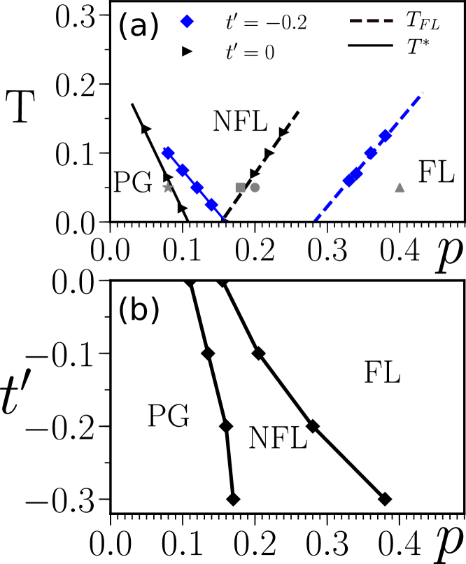
Figure 1: Pseudogap (PG), Non Fermi liquid (NFL) and Fermi liquid (FL) phases of the doped Hubbard model in normal state. (a): Pseudogap temperature $T^{*}$ and Fermi liquid temperature $T_{FL}$ as a function of hole doping value $p$ for two typical $t^{\prime}$ values, $t^{\prime}=0$ (Triangles) and $t^{\prime}=-0.2$ (Diamonds). The finite temperature data points are extrapolated to zero temperature (lines), yielding two critical dopings $p^{*}$ and $p_{FL}$. For example, for $t^{\prime}=-0.2$, $p^{*}\simeq 0.16$ and $p_{FL}\simeq 0.28$. For the definition of $T^{*}$ and $T_{FL}$ please refer to main text and Supplementary Sec. C. The gray symbols mark the data points that are further analyzed in Fig. 4 at $t^{\prime}=-0.2t$. (b): Zero temperature phase diagram in the $p-t^{\prime}$ plane. The above extrapolated $p^{*}$ and $p_{FL}$ define the PG/NFL and NFL/FL phase boundaries respectively.

Phase diagram

We first display two characteristic energy scales of the doped normal state Hubbard model: the pseudogap temperature $T^{*}$, and the Fermi liquid temperature $T_{FL}$, as a function of doping levels $p$ in Fig. 1a. Here $T^{*}$ is defined as the temperature $T$ where the antinodal zero-frequency spectral function starts to decrease with $T$, and $T_{FL}$ is identified as the temperature where the paramagnetic susceptibility (Knight shift) becomes $T$-independent (see Supplementary Fig.S4). Extrapolating $T^{*}$ and $T_{FL}$ to zero, one finds two critical dopings: $p^{*}$ where pseudogap disappears for $p>p^{*}$, and $p_{FL}$ where Fermi liquid emerges for $p>p_{FL}$. Repeating this calculation for several $t^{\prime}$ values, we obtained a zero temperature phase diagram in the $p-t^{\prime}$ plane, as shown in Fig.1b, which consists of three different phases: (1) PG phase in the underdoped regime where $p<p^{*}$ ( and $T^{*}>0$). (2) Canonical FL phase on the heavily overdoped side for $p>p_{FL}$ (where $T_{FL}>0$). (3) Finally, in between PG and FL phases, there exists a NFL phase where the extrapolated $T^{*}$ and $T_{FL}$ both vanish in the $p^{*}<p<p_{FL}$ interval. Namely in the NFL phase, there is no pseudogap at the Fermi level but the physical properties disagree with expectations for a Fermi liquid. It is remarkable that for all the $t^{\prime}$ values we have studied, the NFL resides in a finite range of dopings. In fact, as the value of $|t^{\prime}/t|$ increases, the NFL regime becomes broader in doping, as one can see from Fig.1a. This result suggests that upon hole doping, the pseudogap state does not directly transit to the Fermi liquid phase via a single quantum critical point at zero temperature.

Comparing with experiments, we note that in $\mathrm{La_{2-x}Sr_{x}CuO_{4}(LSCO)}$ compound ($t^{\prime}/t\sim-0.2$), it is found that the PG ends at $p^{*}\simeq 0.18$, and Fermi liquid shows up at $p_{FL}\simeq 0.3$ [where $p_{FL}$ is defined as where the temperature-dependent resistivity becomes $\rho(T)\propto T^{2}$  Cooper et al. (2009); Barišić et al. (2013)]. This is in good agreement with our result that the NFL exists in the doping range $p\in(p^{*}=0.16,p_{FL}=0.28)$ at $t^{\prime}/t=-0.2$. Recall that here the spontaneous symmetry breaking phases, such as the d-wave superconductivity (SC), are suppressed to simulate transport experiments in high magnetic field.

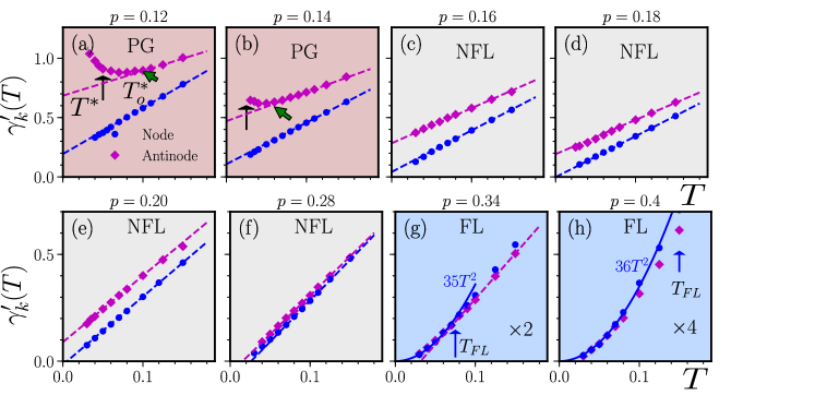
Figure 2: Temperature dependence of the electron scattering rate. Here $\gamma^{\prime}_{k}\equiv-\mathrm{Im}\Sigma^{(2)}(k,\omega=0)$ is shown as a function of temperature $T$ for different dopings. Dashed lines show linear fittings $\gamma^{\prime}_{k}=aT+b$, while solid lines show quadratic fittings $\gamma^{\prime}_{k}=aT^{2}$. For example, at $p=0.18$, for antinode $\gamma^{\prime}_{k}\approx 3.13T+0.17$ and for node $\gamma^{\prime}_{k}\approx 3.45T$ , while $\gamma^{\prime}_{k}\approx 9T^{2}$ for nodal $\gamma^{\prime}_{k}$ at $p=0.4$. Note that in the last two subplots, $\gamma^{\prime}_{k}$ data is enlarged for clarity. The pseudogap temperature $T^{*}$ , and the temperature $T^{*}_{o}$ where $\gamma^{\prime}_{k}$ starts to deviate from linearity are marked by arrows in subplots (a) and (b). In subplots (g) and (h) the Fermi liquid temperature $(T_{FL})$ is also indicated by arrows. For the definition of $T^{*}$ and $T_{FL}$, please refer to main text and Supplementary Sec. C.

$T-$ linear scattering rate

The electronic scattering rate $\gamma_{k}\equiv-\mathrm{Im}\Sigma(k,\omega=0)$ in the NFL phase is the primary focus of this work. We find that in the NFL, the Matsubara data for the self-energy $\Sigma(\mathbf{k},i\omega_{n})$ is consistent with the hypothesis that the imaginary part of the self-energy in real frequency space $\Sigma^{{}^{\prime\prime}}(k,\omega)\equiv\mathrm{Im}\Sigma(k,\omega)$ follows an $\omega/T$ scaling Parcollet and Georges (1999); Varma et al. (1989); Schröder et al. (2000); Schäfer et al. (2021) at low-energies (see Supplementary Fig. S5-S6). Hence we assume that $\Sigma^{{}^{\prime\prime}}(k,\omega)$ can be written as $\Sigma^{{}^{\prime\prime}}(k,\omega)=-T^{\alpha}\phi(\omega/T)-b$ Schäfer et al. (2021); Chen et al. (2019) at low-energies, where $\phi(\omega/T)$ is an analytic function of $\omega/T$, while $\alpha$ and $b$ are constants. With this assumption, the imaginary part of the self-energy at zero-frequency that follows from a second order polynomial extrapolation in Matsubara frequencies $\gamma^{\prime}_{k}\equiv-\mathrm{Im}\Sigma^{(2)}(k,\omega=0)=-\mathrm{Im}[1.875\Sigma(k,i\omega_{0})-1.25\Sigma(k,i\omega_{1})+0.375\Sigma(k,i\omega_{2})]=aT^{\alpha}+b$ will have exactly the same $T-$ dependence of the true scattering rate $\gamma_{k}$, since the scaling hypothesis implies that $\gamma_{k}=\phi(0)T^{\alpha}+b$. Therefore, one can find the exact exponent $\alpha$ describing the $T-$ dependence of $\gamma_{k}$ from analyzing the $\gamma^{\prime}_{k}$ data, despite the fact that the fit leaves the constant coefficient $\phi(0)$ unknown [ if $\Sigma^{{}^{\prime\prime}}(k,\omega)$ is $\omega-$ independent over the frequency range $|\omega|\lesssim 4T$, $\phi(0)\approx a$, see Supplementary Sec.D for details].

Throughout the following, we use the typical value $t^{\prime}=-0.2$ as an example to study the $T-$ linear scattering rate. Fig. 2 displays $\gamma^{\prime}_{k}$ as a function of temperature $T$ for different $p$ values, where one can see that at high temperatures, the scattering rate $\gamma^{\prime}_{k}$ is linear in temperature in a remarkablely large doping range, from underdoped ($p=0.12$, Fig. 2a ) to heavily overdoped side ($p=0.34$, Fig. 2g ) Barišić et al. (2013).

When $T$ is decreased, focusing on the aninodal $\gamma^{\prime}_{k}$ at $\mathbf{k}=(0,\pi)$ as shown in Fig. 2a-b, at small dopings ($p=0.12,0.14$, in the PG), $\gamma^{\prime}_{k}$ deviates from its high temperature $T-$ linearity, developing a prominent upturn when the pseudogap temperature $T^{*}$ is reached. This resembles the upturn seen in the dc resistivity curves in transport experiments Cyr-Choinière et al. (2018), and in other calculations Gull et al. (2010); Sordi et al. (2013), which characterizes the opening of pseudogap. As the doping level $p$ increases, the upturn of $\gamma^{\prime}_{k}$ at the antinode shifts to lower temperatures in the the PG phase, reflecting the decreasing $T^{*}$. Finally, when the NFL phase is reached, a possible upturn of $\gamma^{\prime}_{k}$ moves outside of the acessible temperature range. The linear $T-$ dependence of $\gamma^{\prime}_{k}$ at the antinode extends to $T\rightarrow 0$ , as shown in Fig. 2d. For the node, $\gamma^{\prime}_{k}$ preserves the linear- in-$T$ behavior, crossing the PG -NFL transition. Thus for a typical doping close to $p^{*}$ in the NFL, $p=0.18$ (Fig. 2d) for example, both the node and the antinode display a $T-$ linear scattering rate in the full temperature regime. On the heavily overdoped side, the Landau Fermi liquid paradigm is restored at small $T$ when $p>p_{FL}$. As shown in Fig. 2 g-h, the scattering rates crossover from high $T-$ linearity to a clear $T-$ square behavior  Xu et al. (2013) as $T<T_{FL}$.

In essence, at low dopings $\gamma^{\prime}_{k}$ has upturns that characterize the PG, while at large dopings it follows the $T^{2}$ law that characterizes the FL. In the NFL, where $T^{*}$ and $T_{FL}$ are both vanishingly small, $\gamma^{\prime}_{k}(T)$ obeys $\gamma^{\prime}_{k}(T)=aT+b$ in a broad $T$ range. Nevertheless, we point out that in the NFL, when doping $p$ is close to $p^{*}$ or $p_{FL}$, the precursor effects of pseudogap or Fermi liquid at small $T$ can also break the $T-$ linearity of $\gamma^{\prime}_{k}(T)$ , even if $T^{*}$ or $T_{FL}$ appear to vanish (see Supplementary Fig. S7). As a result, in the $T\rightarrow 0$ limit , $\gamma^{\prime}_{k}(T)=aT+b$ is obeyed only in a part of the NFL regime. For example, at $t^{\prime}/t=-0.2$, while our definition suggests that the NFL exists in $0.16\lesssim p\lesssim 0.28$ at vanishing $T$ (see discussions in Supplementary Sec.E), the perfect linear-in-$T$ behavior of $\gamma^{\prime}_{k}(T)$ [ or equivalently the linear-in-$T$ behavior of $\gamma_{k}(T)$ ] occurs in the doping range of $0.17\lesssim p\lesssim 0.20$ as $T\rightarrow 0$,

Up to now, we have investigated the electron scattering rate $\gamma_{k}=-\mathrm{Im}\Sigma(k,\omega=0)$. In the FL regime, this differs from the quasiparticle scattering rate by a temperature-independent quasiparticle weight $z_{k}$. In the NFL regime, it is worthwhile to investigate the phenomenological marginal Fermi liquid (MFL) interpretation of the scattering rate $1/\tau_{k}=z_{k}\gamma_{k}$ with $\gamma_{k}=-\mathrm{Im}\Sigma(\mathbf{k},\omega)=\alpha\mathrm{max}(|\omega|,\pi T)+b$ Varma et al. (1989); Varma (2020). The procedure for finding $\tau_{k}$ from fitting the Matsubara Green’s function is explained in Supplementary Sec. F. We find $1/\tau_{k}\sim CT$, with $C\in(1\sim 2)$ (see supplementary Fig. S8-S10) for two doping levels, $p=0.18$ and $p=0.2$, in the $T-$ linear regime. We stress that here $C$ is found dependent on doping $p$ and momentum $\mathbf{k}$. It decreases as $p$ increases, contrary to what we found for the electron-scattering rate, which is nearly independent of doping in the NFL regime.

Origin of the NFL and $T-$ linearity

To reveal the physical origin of the $T-$ linear scattering rate in overdoped Hubbard model, we use the Dyson-Schwinger equation of motion (DSEOM) to decompose the self-energy at the two-particle level Gunnarsson et al. (2015); Wu et al. (2017). Simply explained, the essential idea of this approach is to find how collective modes in different channels [spin (sp), charge (ch) or particle-particle (pp)] contribute to the self-energy. As depicted by the Feynman diagram for the spin channel in the insert of Fig. 3b, the self-energy (with Hatree term ${Un}/{2}$ subtracted) can be written as Gunnarsson et al. (2015),

$$\Sigma(k)-\frac{Un}{2}=-\frac{U}{g(k)\beta^{2}N}\sum_{k^{\prime},Q}F_{sp}(k,k^{\prime},Q)g(k^{\prime})g(k)g(k^{\prime}+Q)g(k+Q)$$ (2)

where wave vectors $k$ stand for $k=(\mathbf{k},i\omega_{n})$ and $g(k)$ is the full single particle Green’s function. Here $F_{sp}$ is the full two-particle scattering amplitude in the transverse spin channel. Hence the right-hand side of the above equation can be rewritten in terms of the spin operators $S^{+}_{k}(-Q)=C_{k\uparrow}^{\dagger}C_{k+Q,\downarrow}$, and $S^{-}_{k^{\prime}}(Q)=C_{k^{\prime}+Q\downarrow}^{\dagger}C_{k^{\prime},\uparrow}$,

$$\Sigma(k)=\frac{-U}{g(k)\beta^{2}N}\sum_{k^{\prime},Q}\langle S^{+}_{k}(-Q)S^{-}_{k^{\prime}}(Q)\rangle$$ (3)

and we can introduce a new quantity $\Sigma^{Q}_{sp}(k)=[-U/g(k)]\sum_{k^{\prime}}\langle S^{+}_{k}(-Q)S^{-}_{k^{\prime}}(Q)\rangle$ such that $\Sigma(k)=\sum_{Q}\Sigma^{Q}_{sp}(k)$, which has a clear physical meaning: the ratio $|\mathrm{Im}\Sigma^{Q}_{sp}(k)/\mathrm{Im}\Sigma(k)|$ tracks the relative importance of the spin excitation with the momentum/frequency transfer $Q$ to the electronic scattering. The above analysis can also be straightforwardly applied to charge and particle-particle representations to estimate the impacts of the corresponding two-particle excitations on the self-energy (see Supplementary Sec.I).

In Fig. 3 a, $\mathrm{Im}\Sigma(\mathbf{k},i\omega_{n})$ is shown as a function of $\omega_{n}$ in different states. Focusing on the low-energy scattering, we perform DSEOM decompositions on the imaginary part of the self-energy at the first fermionic Matsubara frequency $\mathrm{Im}\Sigma(k,i\omega_{0})$. The DSEOM decompositions in the spin channel, $\mathrm{Im}\Sigma^{Q}_{sp}(\mathbf{k},i\omega_{0})$ is displayed in Fig. 4 , as a function of $Q=(\mathbf{q},i\Omega_{n})$ for two typical dopings in the $T$-linear regime in NFL, $p=0.18,0.2$. For comparison, the results at $p=0.08$ (PG) and $p=0.4$ (FL) are also shown.

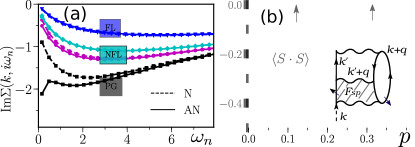
Figure 3: Imaginary part of the self-energy in PG, NFL, FL phases, and the spin-spin correlator $\langle S_{i}\cdot S_{i+1}\rangle$ on nearest neighboring sites $\langle i,i+1\rangle$ as a function of doping $p$. (a): $\mathrm{Im}\Sigma(k,i\omega_{n})$ as a function of $\omega_{n}$ . From bottom to top: $p=0.08$ (PG), $p=0.18$, $p=0.24$ (NFL), and $p=0.4$ (FL). (b): Spin correlator $\langle S_{i}\cdot S_{i+1}\rangle$ at two neighboring sites ($i,i+1$) as a function of doping $p$. Two arrows indicate PG/NFL and NFL/FL phase boundaries respectively. (Insert): Feynman diagram that sketches the Dyson-Schwinger equation of motion decomposition (DSEOM) of the self-energy in the spin channel. Here $U=7t,t^{\prime}=-0.2t,T=0.05t$.

We consider first the $p=0.18$ case. For both antinode [$\mathbf{k}=(0,\pi)$, Fig. 4 A2], and node [$\mathbf{k}=(\pi/2,\pi/2)$, Fig. 4 B2], $-\mathrm{Im}\Sigma^{\mathbf{q}}_{sp}(\mathbf{k},i\omega_{0})$ at different $\mathbf{q}$ are extremely uneven. The AFM wave vector $\mathbf{q}=(\pi,\pi)$ component accounts for most of the low-energy scattering $-\mathrm{Im}\Sigma(\mathbf{k},i\omega_{0})$. This means that in the NFL, most of the electronic scatterings are due to AFM fluctuations, since $\Sigma^{\mathbf{q}}_{sp}(k)\propto\sum_{k^{\prime}}\langle S^{+}_{k}(-\mathbf{q})S^{-}_{k^{\prime}}(\mathbf{q})\rangle$. Moreover, from Fig. 4 C2, one learns from the frequency decomposition that the $\Omega=0$ component dominates, suggesting the long-lived nature of the well-defined AFM fluctuations at this doping.

At a larger doping $p=0.20$, the weight of the $\mathbf{q}\neq(\pi,\pi)$ components grows, as shown in Fig. 4[A3, B3]. However the predominant role of the $\mathbf{q}=(\pi,\pi)$ mode is not changed. In fact, we find that the $\mathbf{q}=(\pi,\pi)$ component always has the largest contribution to $-\mathrm{Im}\Sigma^{\mathbf{q}}_{sp}(\mathbf{k},i\omega_{0})$ among different $\mathbf{q}$ in the NFL, even when $p$ is further increased (see Supplementary Fig. S13). This result is somewhat surprising, as one would intuitively expect negligible AFM correlations in the overdoped regime. To clarify his problem, in Fig. 3b we plot the spin-spin correlator $\langle S_{i+1}\cdot S_{i}\rangle$ between a pair of neighboring sites $(i,i+1)$ as a function of doping $p$. This shows that, although largely reduced by doping, the strength of AFM correlations remains significantly non-zero in the NFL. For example, at $p=0.2$, $\langle S_{i+1}\cdot S_{i}\rangle\approx-0.06$, which is about $40\%$ of the value at $p=0.08$ in the PG. Neutron scattering studies on LSCO show that at $p=0.25$ in the NFL, the dynamical magnetic susceptibility still has fairly large intensity at finite energy, whose magnitude is about half of that at $p=0.125$ in the PG Wakimoto et al. (2007). Resonant inelastic scattering studies also reveal the persistence of spin excitations in the overdoped regime Le Tacon et al. (2013). This emphasizes again that the short-ranged AFM correlations should not be overlooked in the overdoped regime.

The decompositions for the PG and the FL are shown, respectively, in the first and last columns of Fig. 4. In the PG, $-\mathrm{Im}\Sigma^{Q}_{sp}(\mathbf{k},i\omega_{0})$ is similar to the NFL case, revealing again the importance of scattering off AFM fluctuations Gunnarsson et al. (2015); Wu et al. (2017); Cyr-Choinière et al. (2018). By contrast, in the FL phase, a clear distinction between the NFL and PG cases is observed: $-\mathrm{Im}\Sigma^{\mathbf{q}/\Omega_{n}}_{sp}(k)$ with different $\mathbf{q}/\Omega_{n}$ are more or less comparable. There is no individual mode in $\mathbf{q}/\Omega_{n}$ space that provides a dominant contribution to scattering. This is expected, since scattering in Fermi liquids should be seen as single-particle collisions rather than scattering off collective modes. Hence the two-particle spin representation becomes inappropriate to identify the source of scattering in the FL.

We also performed DSEOM decompositions in other channels, and found no indication of any significant charge or particle-particle collective modes in the NFL (see Supplementary Sec. I and Fig. S12). Therefore we conclude that in the NFL, most of the $T-$ linear electronic scattering comes from AFM fluctuations.

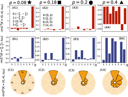
Figure 4: Dyson-Schwinger equation of motion decomposition of the self-energy in spin channel, $\mathrm{Im}\Sigma^{\mathbf{q}/\Omega_{n}}_{sp}(\mathbf{k},i\omega_{0})$ at different dopings. (A1-A4): $\mathrm{Im}\Sigma^{\mathbf{q}}_{sp}(\mathbf{k},i\omega_{0})$ as a function of transfer momentum $\mathbf{q}$ for the antinode [$\mathbf{k}=(0,\pi)$]. (B1-B4): $\mathrm{Im}\Sigma^{\mathbf{q}}_{sp}(\mathbf{k},i\omega_{0})$ as a function of transfer momentum $\mathbf{q}$ for the node [$\mathbf{k}=(\pi/2,\pi/2)$]. (C1-C4): $\mathrm{Im}\Sigma^{\Omega_{n}}_{sp}(k,i\omega_{0})$ as a function of transfer frequencies $\Omega_{n}=2n\pi T$ for the antinode [$\mathbf{k}=(0,\pi)$]. Values of indiced transfer momenta $\mathbf{q}$ are labeled in A1 and A2. $\mathrm{Im}\Sigma^{\Omega_{n}}_{sp}(k,i\omega_{0})$ for the node, not shown here, is similar to that of the antinode [C1-C4].

Discussion

In recent ARPES measurements of Bi2212, it is found that the ARPES spectra near $p^{*}$ can be well fitted by a marginal Fermi liquid form for the self-energy $-\mathrm{Im}\Sigma(k,\omega)=T\phi(\omega/T)+b$ Chen et al. (2019), which supports our assumption of $\omega/T$ scaling in the NFL state. Moreover, we note that $\gamma^{\prime}_{k}(T)$ has similar slopes in $T$ at the node and at the antinode, which means that the inelastic part ($T-$ dependent part) of the scattering rates, $\gamma^{in}_{k}(T)\equiv\gamma^{\prime}_{k}(T)-\gamma^{\prime}_{k}(0)$ are isotropic in our study. For example at $p=0.18$, $\gamma^{in}_{N}(T)/\gamma^{in}_{AN}(T)\approx 1.1$, as shown in Fig. 2. This agrees with early ARPES results Kaminski et al. (2005) and very recent angle-dependent magnetoresistance (ADMR) experiments on LSCO Grissonnanche et al. (2021). We note that an immediate consequence of $\gamma_{k}(T)$ being perfectly linear-in-T in the NFL is that the dc resistivity $\rho_{T}$ without vertex corrections, can also have linear temperature dependence (see Supplementary Sec. G).

Where does the linear $T-$ dependence come from? In the case of phonons, when temperature $T$ is larger than about one third of the Debye frequency Hartnoll and Mackenzie (2021), The scattering rate increases like $T$ because the number of bosonic scatterers grows linearly with $T$ Sadovskii (2021). In the case of an antiferromagnetic QCPMillis (1993); Gegenwart et al. (2008); Löhneysen et al. (2007); Xu et al. (2020); Dumitrescu et al. (2021), the characteristic spin fluctuation frequency plays the role of the Debye frequency in the phonon case and it indeed vanishes. However it does not explain the $T-$linear scattering rate in the case of weak interactions, since the electrons - spin fluctuations scattering will be strong only at hot spots on the Fermi surface so that, barring disorder effects Rosch (1999), the resulting resistivity will be short-circuited by Fermi-liquid-like portions of the Fermi surface Hlubina and Rice (1995).

For the strong interaction, $U=7t$ that we considered, it can be speculated that the lack of well-defined fermion quasiparticles leads to spin fluctuations with overall vanishing characteristic frequency. Then, the argument that the number of scatterers scales like $T$ should hold. Since the magnetic correlation length is small in the over-doped regime Kastner et al. (1998), the electrons on remains of the Fermi surface can be all effectively scattered. Then the argument that the linear $T-$ dependence of the scattering rate is isotropic on the Fermi surface will also hold. In this case, dimensional analysis and Kanamori-Brückner screening suggest (see Sec. L of Supplementary) that the coefficient of the linear $T-$ dependence of the scattering rate can be of order unity. But it does not need to be unity. In fact, we find a number about equal to three for the electron scattering rate, and about ($1\sim 2$) for quasiparticle scattering rate with the current parameters. So we call the strong-interaction case that we studied, a “nearly Planckian liquid” and we argue that Planckian dissipation likely not to be a fundamental limit to the inelastic electron scattering rate Sadovskii (2021); Nicholas et al. (2021).

Conclusion

To conclude, we investigated the two-dimensional Hubbard model in the intermediate to strong interaction limit where a non-Fermi liquid phase is found to exist in the overdoped regime. We found that the electronic scattering rate $\gamma_{k}(T)$ can have a perfectly linear $T-$ dependence when doping $p$ is close to the pseudogap critical doping $p^{*}$. We also discovered that the antiferromagnetic fluctuations are responsible for the $T-$ linear electron scattering at low temperatures.

Method

Our results for the two-dimensional Hubbard model are obtained using the dynamical cluster approximation (DCA) Maier et al. (2005b), which is a cluster extension of the dynamical mean-field theory (DMFT). (See Supplementary Secs. A to C for details) The DCA method captures short-ranged spatial correlations within the cluster exactly, while longer range spatial correlations are taken into account by a dynamical mean-field, which can be represented by a momentum- and frequency- dependent Weiss field $g_{0}(\mathbf{k},i\omega_{n})$. The effective cluster impurity problem starting from $g_{0}(\mathbf{k},i\omega_{n})$ is solved by the Hirsch-Fye quantum Monte carlo method Hirsch and Fye (1986), which in general has a slightly better average sign as compared to the continuous-time quantum Monte Carlo method (CTQMC) Gull et al. (2011). Here we use a discrete imaginary-time step $\Delta\tau=0.071$. We have carefully verified that this finite $\Delta\tau$ is small enough so that the Trotter errors do not affect our result and conclusion, see Supplementary Fig. S2. Comparison with CTQMC result also shows that our conclusion is not changed in the $\Delta\tau\rightarrow 0$ limit, see Supplementary Fig. S3. In this work, we typically use 60 DCA self-consistency iterations to get a converged Weiss field $g_{0}(\mathbf{k},i\omega_{n})$, or equivalently a converged self-energy $\Sigma(\mathbf{k},i\omega_{n})$. In the eight-site DCA approximation, the lattice self-energy is approximated by a patchwise-constant self-energy $\Sigma(\mathbf{k},i\omega_{n})$ in the Brillouin zone with eight different patches as shown in Supplementary Fig. S1. Note that the antinodal and nodal regions are in distinct patches in this eight-site cluster scheme. We have verified that the $T-$ linear scattering rate also appears in four-site DCA, and $4\times 4$ -site DCA calculations, namely, it can be checked explicitly for $T>0.1$ that our results are insensitive to the cluster size, see Supplementary Figs. S14-S15.

Supplementary Materials: Non-Fermi liquid phase and linear-in-temperature scattering rate in overdoped two dimensional Hubbard model

Wéi Wú^1∗, Xiang Wang¹ & A.-M. S.Tremblay²

Appendix A Geometry of the DCA clusters

The different DCA clusters that we have used are shown in the following Fig. S1a shows the DCA patches in momentum space for the 8-site cluster.

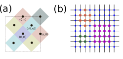
Figure S1: Geometries of the DCA clusters used in this work (a): DCA patches in momentum space for the eight-site cluster. (b): Geometries of the $4-$, $8-$, and $16-$ site DCA clusters used in this work.

Appendix B Analysis on the Trotter errors of the HFQMC solver

In this work, we typically use $\Delta\tau=0.071$ in the Hirsch-Fye impurity solver Hirsch and Fye (1986). We have carefully verified that this finite $\Delta\tau$ is small enough that the Trotter errors do not affect our result and conclusion, as shown in Fig. S2. Comparison with CTQMC results also shows that our conclusion is not changed in the $\Delta\tau\rightarrow 0$ limit, as shown in Fig. S3.

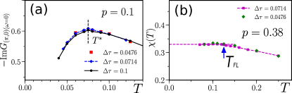
Figure S2: The pseudogap temperature $T^{*}$ and Fermi liquid temperature $T_{FL}$ are converged in HFQMC at $\Delta\tau=0.0714$. (a): The imaginary part of the antinodal Green’s function $-\mathrm{Im}G_{(\pi,0)}(\omega=0)$ shows a maximum as temperature $T$ decreases at the same $T$ for $\Delta\tau$ = 0.1 (circle), 0.0714 (diamond), and 0.0476 (square), suggesting our $T^{*}$ data in the main text at $\Delta\tau=0.0714$ is converged. (b): The paramagnetic susceptibility $\chi(T)$ saturates at the same $T$ for $\Delta\tau$ = 0.0714 (square), and 0.0476 (diamond), suggesting that our $T_{FL}$ data at $\Delta\tau=0.0714$ is also converged. Here $U=7t,t^{\prime}=-0.2t$.

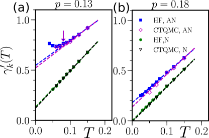
Figure S3: Comparison of the HFQMC and CTQMC results for the electronic scattering rate $\gamma^{\prime}_{\mathbf{k}}(T)$ . (a): At doping level $p=0.13$ in the PG. (b): At doping level $p=0.18$ in the NFL. For the node, the differences in $\gamma^{\prime}_{\mathbf{k}}(T)$ between CTQMC and HFQMC are negligible at both dopings. For the antinode, $\gamma^{\prime}_{\mathbf{k}}(T)$ of CTQMC is slightly smaller than that of HFQMC at low temperatures. In the PG ($p=0.13$), the temperatures $T^{*}_{o}$ where $\gamma^{\prime}_{\mathbf{k}}(T)$ starts to deviate from linearity (marked by arrows) are essentially the same for CTQMC and HFQMC. In the NFL ($p=0.18$), CTQMC and HFQMC results both show $T-$ linear antinodal $\gamma^{\prime}_{\mathbf{k}}(T)$, despite the slightly larger slope of the antinodal $\gamma^{\prime}_{\mathbf{k}}(T)$ of CTQMC. Hence our conclusion drawn from $\Delta\tau=0.0714$ result that for $0.17\lesssim p\lesssim 0.20$, the electronic scattering rate is linear in $T$ is not changed when $\Delta\tau\rightarrow 0$ is extrapolated. Here $U=7t,t^{\prime}=-0.2t$.

Appendix C Pseudogap temperature $T^{*}$ and Fermi liquid temperature $T_{FL}$

In this work the pseudogap $T^{*}$ is identified as the temperature where the antinodal zero- frequency spectral function ( obtained by extrapolation Wu et al. (2018) ) displays a maximum. Thus below $T^{*}$, the antinodal spectral intensity decreases, denoting the opening of a pseudogap. $T_{FL}$ is defined as the temperature where the paramagnetic susceptibility $\chi(T)$ ( Knight shift ) saturates while decreasing temperature $T$, as shown in  Fig. S4.

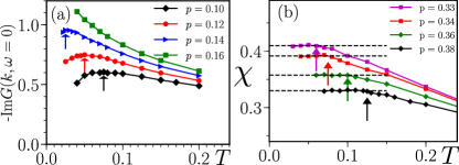
Figure S4: Pseudogap temperature $T^{*}$ and Fermi liquid temperature $T_{FL}$ at $U=7t,t^{\prime}=-0.2t$ for various dopings (a): Pseudogap temperature $T^{*}$ is defined as the temperature where $-\mathrm{Im}G(k,\omega=0)$ at $k=(0,\pi)$ reaches a maximum. Here $-\mathrm{Im}G(k,\omega=0)$ is obtained by linear fitting in Mastsubara frequency space using Green’s functions at the lowest two frequencies. (b): Fermi liquid temperature $T_{FL}$ is defined as the temperature where the paramagnetic susceptibility $\chi(T)=\frac{1}{N}\sum_{i,j}\int_{0}^{\beta}\langle S_{i}(\tau)\cdot S_{j}(0)\rangle d\tau$ saturates when decreasing $T$. The dashed lines denote the average $\chi(T)$ values of the last four $T$ points for each doping. Here the numerical data of $\chi(T)$ is actually obtained by computing the paramagnetic response to a small uniform magnetic field to the system. The inducing magnetic field is chosen small enough to ensure a linear response. Arrows in the two subplots indicate $T^{*}$ (Left) and $T_{FL}$ (Right) respectively.

Appendix D $\omega/T$ scaling of the self-energy

In Fermi liquids the imaginary part of the self-energy obeys $\omega/T$ scaling. It can occur more generally in strongly correlated systems that physical quantities display $\omega/T$ scaling when the relevant characteristic energy scales vanishes Schröder et al. (2000); Sachdev (2011); Parcollet and Georges (1999); Gegenwart et al. (2008). We find that in the NFL regime of the overdoped Hubbard model, numerical data suggests $\omega/T$ scaling behavior of the imaginary part of the self-energy $\mathrm{Im}\Sigma(\mathbf{k},\omega)$ in real-frequency space, as discussed below.

It has been shown that $\omega/T$ scaling of $\Sigma^{{}^{\prime\prime}}(\mathbf{k},\omega)\equiv\mathrm{Im}\Sigma(\mathbf{k},\omega)$ at low-energies leads to $\tau/\beta$ scaling Dumitrescu et al. (2021) near $\tau\sim 0.5\beta$ when translated in imaginary time $\Sigma(\mathbf{k},\tau)$. This is because,

$$\Sigma(\mathbf{k},\tau)=\int\Sigma^{{}^{\prime\prime}}(k,\omega)K_{\beta}(\omega,\tau)\frac{d\omega}{\pi}$$ (S1)

$$=\int\frac{\Sigma^{{}^{\prime\prime}}(k,\omega)e^{-\tau\omega}}{1+e^{\beta\omega}}\frac{d\omega}{\pi}\ =\frac{T}{\pi}\int\frac{\Sigma^{{}^{\prime\prime}}(k,\omega)e^{-\frac{\tau}{\beta}\times(\omega/T)}}{1+e^{\omega/T}}d\frac{\omega}{T}$$ (S2)

i.e., the integral kernel $K_{\beta}(\omega,\tau)$ can be rewritten as a function of $\tau/\beta$ and $\omega/T$. Therefore when the $\omega-$ dependence of $\Sigma^{{}^{\prime\prime}}(\mathbf{k},\omega)$ can be expressed as a function of $\omega/T$, $\Sigma(\mathbf{k},\tau)$ will follow $\tau/\beta$ scaling. Note that when $\tau\sim 0.5\beta$, the integral kernel $K_{\beta}(\omega,\tau)=e^{-\tau\omega}/(1+e^{\beta\omega})$ is a bell-shaped function in $\omega$, which essentially collects the low-energy weight of $\Sigma^{{}^{\prime\prime}}(\mathbf{k},\omega)$ between $-4T\lesssim\omega\lesssim 4T$.

Here we use a slightly different method to show the $\omega/T$ scaling behavior of $\Sigma^{{}^{\prime\prime}}(\mathbf{k},\omega)$ from $\Sigma(\mathbf{k},\omega_{n})$ data in Matsubara frequencies. Fitting $\mathrm{Im}\Sigma(\mathbf{k},i\omega_{n})$ data to the first three Mastsubara frequencies, $\mathrm{Im}\Sigma(\mathbf{k},i\omega_{0})$, $\mathrm{Im}\Sigma(\mathbf{k},i\omega_{1})$, $\mathrm{Im}\Sigma(\mathbf{k},i\omega_{2})$ to a quadratic function of $\omega_{n}$, and then extrapolating to small frequencies $\omega_{m}$ ( $\omega_{m}<\omega_{0}=\pi T$ ), we obtain an extrapolated self-energy $\mathrm{Im}\Sigma^{(2)}(\mathbf{k},i\omega_{m})$ that is equal to,

$$\mathrm{Im}\Sigma^{(2)}(\mathbf{k},i\omega_{m})=\int\Sigma^{{}^{\prime\prime}}(k,\omega)K_{T}(\omega,\omega_{m})\frac{d\omega}{\pi}$$ (S3)

with the integral kernel $K_{T}(\omega,\omega_{m})$ given by,

$$K_{T}(\omega,\omega_{m})=A(\omega,T)\omega_{m}^{2}+B(\omega,T)\omega_{m}+C(\omega,T)$$

$$A(\omega,T)=\mathrm{Im}[\frac{1}{8\pi^{2}T^{2}(\omega-i\pi T)}-\frac{1}{4\pi^{2}T^{2}(\omega-3i\pi T)}+\frac{1}{8\pi^{2}T^{2}(\omega-5i\pi T)}]$$

$$B(\omega,T)=\mathrm{Im}[-\frac{1}{\pi T(\omega-i\pi T)}+\frac{3}{2\pi T(\omega-3i\pi T)}-\frac{1}{2\pi T(\omega-5i\pi T)}]$$

$$C(\omega,T)=\mathrm{Im}[\frac{15}{8(\omega-i\pi T)}-\frac{5}{4(\omega-3i\pi T)}+\frac{3}{8(\omega-5i\pi T)}].$$ (S4)

The kernel $K_{T}(\omega,\omega_{m})$ is also a bell-shaped function in energy $\omega$ whose weight is mainly between $-4T\lesssim\omega\lesssim 4T$, when $\omega_{m}$ are small ( $|\omega_{m}|<\pi T$, see Fig. S5). Note that $K_{T}(\omega,\omega_{m})$ can be rewritten as a function of $\omega/T$ and $\omega_{m}/T$,

$$K_{T}(\omega,\omega_{m})=\kappa(\omega/T,\omega_{m}/T).$$

Thus $\mathrm{Im}\Sigma^{(2)}(\mathbf{k},i\omega_{m})$ obtained from the integral of equation (S3) exhibits $\omega_{m}/T$ scaling at small $\omega_{m}$, if $\Sigma^{{}^{\prime\prime}}(\mathbf{k},\omega)$ has $\omega/T$ scaling at low-energies .

According to the above analysis, one can therefore extrapolate $\Sigma(\mathbf{k},i\omega_{n})$ using a second order polynomial fit in Matsubara frequency space to obtain $\mathrm{Im}\Sigma^{(2)}(\mathbf{k},i\omega_{m})$ at small $\omega_{m}$ and verify whether $\Sigma^{{}^{\prime\prime}}(\mathbf{k},\omega)$ obeys $\omega/T$ scaling at low-energies. Our DCA result is shown in Fig. S6 where one can see that for $p=0.18$ in the NFL, $\mathrm{Im}\Sigma^{(2)}(\mathbf{k},i\omega_{m})$ (normalized by $\mathrm{Im}\Sigma^{(2)}(\mathbf{k},i\omega_{m}=0)$) at different temperatures $T$ indeed collapses nicely to a single scaling function of $\omega_{m}/T$ . In other words, $\mathrm{Im}\Sigma^{(2)}(\mathbf{k},i\omega_{m})/\mathrm{Im}\Sigma^{(2)}(\mathbf{k},i\omega_{m}=0)=S(\omega_{m}/T)$ holds at different $T$ for small $\omega_{m}$, where $S(\omega_{m}/T)$ appears to be essentially a linear function of $\omega_{m}/T$ according to Fig. S6. This result unambiguously shows that in the NFL, $\Sigma^{{}^{\prime\prime}}(\mathbf{k},\omega)$ does follow $\omega/T$ scaling at low-energies.

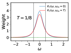
Figure S5: The $K_{T}(\omega,\omega_{m})$ function at two different $\omega_{m}$. Vertical dashed lines show $\omega=-4T$ and $\omega=4T$ respectively.

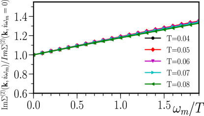
Figure S6: $\omega_{m}/T$ scaling of the imaginary part of the extrapolated self-energy $\mathrm{Im}\Sigma^{(2)}(\mathbf{k},i\omega_{m})$ at small imaginary frequencies $\omega_{m}$ . $\mathrm{Im}\Sigma^{(2)}(\mathbf{k},i\omega_{m})$ is obtained from a second order polynomial extrapolation of $\mathrm{Im}\Sigma(\mathbf{k},i\omega_{n})$ in Matsubara frequencies. Here $u=7t,t^{\prime}=-0.2t,p=0.18$ and $\mathbf{k}=(\pi,0)$.

We have shown above that the energy dependence of $\mathrm{Im}\Sigma(k,\omega)$ follows $\omega/T$ scaling at low-energies in the NFL. If we assume that $\Sigma^{{}^{\prime\prime}}(k,\omega)\equiv\mathrm{Im}\Sigma(k,\omega)$ can be written as $\Sigma^{{}^{\prime\prime}}(k,\omega)=-T^{\alpha}\phi(\omega/T)-b$, where $\phi(\omega/T)$ is an unknown analytic function of $\omega/T$, and $b$ is a constant, it is straightforward to prove that $\mathrm{Im}\Sigma^{(n)}(k,\omega=0)$ extrapolated with an $n-$ order polynomial fit of $\mathrm{Im}\Sigma(k,i\omega_{n})$ in Matsubara frequency space will have the same $T-$ dependence as the true scattering rate $-\mathrm{Im}\Sigma(k,\omega=0)$. To be specific, take the second order extrapolation

$$\gamma^{\prime}_{k}\equiv-\mathrm{Im}\Sigma^{(2)}(k,i\omega_{m}=0)=-\mathrm{Im}[1.875\Sigma(k,i\omega_{0})-1.25\Sigma(k,i\omega_{1})+0.375\Sigma(k,i\omega_{2})],$$

then the integral kernel $K_{T}(\omega,\omega_{m}=0)$ reads,

$$K_{T}(\omega,0)=C(\omega,T)=\sum_{n=1}^{n=3}\frac{c_{n}\omega_{n}}{\omega^{2}+{\omega_{n}}^{2}} c_{1,2,3}=[1.875,-1.25,0.375]$$ (S5)

(See also Eq. S4 and Fig S5). Hence, as long as $\omega/T$ scaling applies in the range $|\omega|<\omega_{M}\approx 4T$ for $\Sigma^{{}^{\prime\prime}}(k,\omega)$, we have for $\gamma^{\prime}_{k}$

$$\gamma_{k}^{\prime}=\frac{1}{\pi}\int_{-\omega_{M}}^{\omega_{M}}\sum_{n=1}^{n=3}\frac{c_{n}\omega_{n}}{\omega^{2}+{\omega_{n}}^{2}}[T^{\alpha}\phi(\frac{\omega}{T})+b]d\omega$$ (S6)

$$=\frac{T^{\alpha}}{\pi}\int_{-\omega_{M}/T}^{\omega_{M}/T}\sum_{n=1}^{n=3}\frac{c_{n}(2n+1)\phi(\frac{\omega}{T})}{(\frac{\omega}{T})^{2}+(2n+1)^{2}\pi^{2}}d(\frac{\omega}{T})+b$$ (S7)

$$=aT^{\alpha}+b$$ (S8)

where the above integral over $\omega/T$ yields a constant $a\pi$ because the integrand is a function of $\omega/T$. Comparing to the true electronic scattering rate $\gamma_{k}\equiv-\Sigma^{{}^{\prime\prime}}(k,\omega=0)=\phi(0)T^{\alpha}+b$, we see that $\gamma^{\prime}_{k}=aT^{\alpha}+b$ indeed captures correctly the $T-$ dependence of $\gamma_{k}$.

Note that if $\Sigma^{{}^{\prime\prime}}(k,\omega)$ is constant over the frequency range $|\omega|\lesssim\omega_{M}\approx 4T$, or namely, if $\phi(\omega/T)$ becomes $\omega-$ independent in $|\omega|\lesssim\omega_{M}$, the above integral will lead to $\phi(0)\approx a$. Thus $\gamma^{\prime}_{k}\approx\gamma_{k}$ in such situation. For the marginal Fermi liquid selfenergy Varma et al. (1989), $\mathrm{Im}\Sigma(\mathbf{k},\omega)=\alpha\mathrm{max}(|\omega|,\pi T)$ which becomes $\omega-$ dependent when $|\omega|>\pi T$. Therefore in general $\phi(0)<a$ can be speculated for marginal Fermi liquid, and $\gamma^{\prime}_{k}$ should have a slope in $T$ slightly larger than that of the true electron scattering rate $\gamma_{k}$.

Appendix E $T-$ linearity of the scattering rate in the NFL phase.

In the NFL, the electronic scattering rate $\gamma^{\prime}_{k}(T)$ can in general display a linear temperature dependence $\gamma^{\prime}_{k}(T)=aT+b$ . However, in the underdoped cases the temperature where $\gamma^{\prime}_{k}(T)$ starts to deviate from linearity (marked as $T^{*}_{o}$ in Fig. 2a-b) is higher than $T^{*}$. This means that when $p$ just surpasses $p^{*}$, $\gamma^{\prime}_{k}(T)$ can still can deviate from linearity (since $T^{*}_{o}$ is finite), although the PG temperature $T^{*}$ vanishes. Extrapolating $T^{*}_{o}$ to zero, as shown in Fig. S7, we find that the minimal doping where $\gamma^{\prime}_{k}(T)$ can preserve $T-$ linearity in the $T=0$ limit is around $p_{L}\simeq 0.17$, which is slightly larger than $p^{*}=0.16$ where the pseudogap ends.

Note that in experiments, there are usually different ways to define $T^{*}$. For example, sometimes $T^{*}$ is defined as the temperature where the dc resistivity $\rho(T)$ departs from linearity Cyr-Choinière et al. (2018). This effectively defines $T^{*}_{o}$ as the pseudogap temperature, which would lead to a slightly different $p^{*}\equiv p_{L}=0.17$.

On the overdoped side of the NFL, we find that when $p>0.2$, $\gamma^{\prime}_{k}(T)$ can also deviate from linear-in-$T$ behavior at very small $T$ owing to the onset of Fermi liquid physics, even though there is no finite $T_{FL}$. As shown in Fig. 2f for $p=0.28$, extrapolating $\gamma^{\prime}_{k}(T)$ to zero $T$ using $\gamma^{\prime}_{k}(T)=aT+b$ leads to a nonphysical $\gamma^{\prime}_{k}(T=0)<0$, signaling the failure of a purely linear function to describe $\gamma^{\prime}_{k}(T)$ in the $T\rightarrow 0$ limit. Hence for $p>0.2$, higher order corrections, such as quadratic or cubic terms could develop in $\gamma^{\prime}_{k}(T)$ at small $T$, as a result of Fermi liquid onset. To summarize the above analysis, we find that the scattering rate $\gamma^{\prime}_{k}(T)$ in the NFL phase displays perfect $T-$ linear behavior as $T\rightarrow 0$ in the doping range of $0.17\lesssim p\lesssim 0.20$ for $t^{\prime}/t=-0.2$.

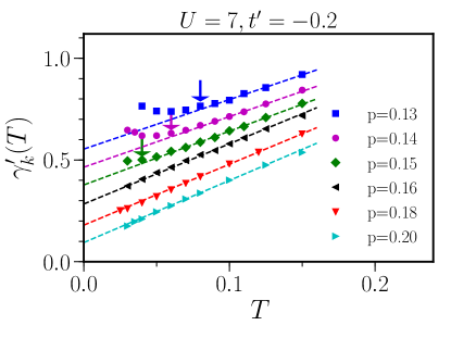
Figure S7: Antinodal scattering rate $\gamma^{\prime}_{k}(T)$ [$\mathbf{k}=(0,\pi)$] as a function of temperature $T$ for various dopings. Arrows indicate the temperature $T^{*}_{o}$, where $\gamma^{\prime}_{k}(T)$ starts to deviate from linearity. Extrapolating $T^{*}_{o}$ to zero, we estimate that the minimal doping where $\gamma^{\prime}_{k}(T)$ is linear in the $T\rightarrow 0$ limit is $p\approx 0.17$. Dashed lines show linear fits (least square) of $\gamma^{\prime}_{k}(T)$ in the temperature range $T=(0.09-0.125)$.

Appendix F Quasiparticle scattering rate

In the main text, we have investigated the electronic scattering rate $\gamma_{k}\equiv-\mathrm{Im}\Sigma(\mathbf{k},\omega=0)$. To study the the quasiparticle scattering rate or inverse quasiparticle life-time $1/\tau_{k}=z_{k}\gamma_{k}$ , one needs to also find out the quasiparticle weight $z_{k}$. To obtain $z_{k}$, here we assume that the Green’s functions at $k_{F}$ have a quasiparticle form as $G(\mathbf{k}_{F},\omega)=z_{k}/[\omega-iz_{k}\mathrm{Im}\Sigma(\mathbf{k}_{F},\omega)]$ at low-energies, and the imaginary part of the selfenergy at low-energies is assumed to be of the marginal Fermi liquid (MFL) type, $-\mathrm{Im}\Sigma(\mathbf{k},\omega)=\alpha\mathrm{max}(|\omega|,\pi T)+b$ Varma (2020). With this hypothesis, we fit the Green’s function data in imaginary time space $G(\mathbf{k}_{F},\tau)$ by,

$$G(\mathbf{k}_{F},\tau)=\int d\omega\frac{A(\mathbf{k}_{F},\omega)e^{-\omega\tau}}{1+e^{-\omega\beta}}$$

$$A(\mathbf{k}_{F},\omega)=-\frac{1}{\pi}\frac{\alpha\mathrm{max}(|\omega|,\pi T)+b}{(\omega/z_{k})^{2}+[\alpha\mathrm{max}(|\omega|,\pi T)+b]^{2}}$$ (S9)

in vicinity the of $\tau\sim 0.5\beta$ [to filter out the low-energy behaviors of $G(\mathbf{k}_{F},\omega)$] and to find out the optimal free parameters $z_{k}$ and $\alpha$. The value of the constant $b$ is fixed as the extrapolated value of $\gamma^{\prime}_{\mathbf{k}}(T)$ in the $T\rightarrow 0$ limit from Fig. 2. Therefore the quasiparticle scattering rate $1/\tau_{k}$ can be identified as $1/\tau_{k}=\alpha z_{k}\pi T+bz_{k}$, as shown in Fig. S8.  Fig. S9 shows $1/\tau_{k}$ as a function of $T$ in the $T-$ linear regime, i.e., $p=0.18$ and $p=0.20$. One can clearly see that at these dopings, $1/\tau_{k}\simeq CT$, with $C\sim(1\sim 2)$, namely the inverse quasiparticle lifetime is proportional to absolute temperature $T$ with a coefficient $C$ close to unit. We would like to stress that here the value of $C$ is apparently dependent on the doping level, and is different between node and antinode.

Performing numerical analytic continuations (such as the maximum entropy method (MEM)) on the Green’s functions $G(\mathbf{k},i\omega_{n})$, one can obtain the spectral functions $A(\mathbf{k},\omega)$, and identify the quasiparticle scattering rate $1/\tau_{k}$ as the half width at half maximum (HWHM) of the low-energy peak of $A(\mathbf{k},\omega)$. Fig. S10 shows MEM result Bergeron and Tremblay (2016) on the $T-$ dependence of $1/\tau_{k}$ , which suggests $1/\tau_{k}\sim 2.5T$ for antinode at $p=0.18$. This is in good agreement with the result from fitting the Green’s function $G(\mathbf{k}_{F},\tau)$, which suggests $1/\tau_{k}\sim 2.2T$ for antinode at $p=0.18$ in Fig. S9.

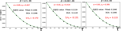
Figure S8: Fitting the Green’s function $G(\mathbf{k},\tau)$ near $\tau\sim 0.5\beta$ with a MFL type of self-energy in theNFL. Curves show fitted $G(\mathbf{k}_{F},\tau)$ using optimized $\alpha$ and $z_{k}$ (shifted by $G(\mathbf{k}_{F},\tau=0.5\beta)$, see Eq. S9), while symbols are DCA data points. From left to right: $T=0.08,0.06,0.05$. Here $U=7t,t^{\prime}=-0.2t,p=0.18$ and $\mathbf{k}_{F}\approx(\pi,0.20)$, in the antinodal (AN) direction. The optimized free parameters $\alpha$, $z_{k}$, and quasiparticle scattering rate $1/\tau_{k}$ are labeled in corresponding subplots. See also Fig. S9.

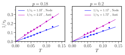
Figure S9: Quasiparticle scattering rate $1/\tau_{k}=-z_{k}\mathrm{Im}\Sigma(k,\omega=0)$ as a function of temperature $T$ in NFL. Here $U=7t,t^{\prime}=-0.2t,p=0.18$. (a): For $p=0.18$ (b): For $p=0.20$. $1/\tau_{k}$ is obtained by fitting the Green’s function $G(\mathbf{k}_{F},\tau)$, see Fig. S8.

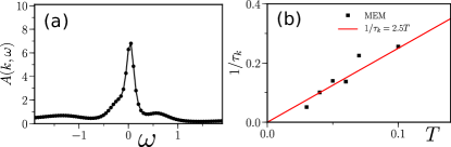
Figure S10: Spectral function $A(k,\omega)$ and quasiparticle scattering rate $1/\tau_{k}$ as a function of temperature $T$ by maximum entropy method analysis (MEM) in the NFL. (a): Spectral function $A(\mathbf{k},\omega)$ at $p=0.18,T=0.06$ (b): Quasiparticle scattering rate $1/\tau_{k}$ in the antinodal direction. Here $U=7t,t^{\prime}=-0.2t,p=0.18$, $\mathbf{k}\approx(\pi,0.20)$.

Appendix G Temperature dependence of the dc resistivity

In this work, we have concentrated on the single-particle properties of the doped Hubbard model. The dc conductivity without vertex correction can be written as,

$$\sigma_{xx}=-2\pi\sum_{\mathbf{k}}\big{(}\frac{\partial\epsilon_{k}}{\partial k_{x}}\big{)}^{2}\int d\omega\frac{\partial f(\omega)}{\partial\omega}A^{2}(\mathbf{k},\omega)=\sum_{\mathbf{k}}\sigma_{\mathbf{k}}.$$ (S10)

Thus, the dc conductivity can be interpreted as the series addition of conductivities $\sigma_{\mathbf{k}}$ (parallel addition of resistivities) defined for each value of wave vector $\mathbf{k}$. A rigorous calculation of the conductivities $\sigma_{\mathbf{k}}$ requires the inclusion of vertex corrections. Assuming that vertex corrections do not modify the linear dependence of the scattering rate that we found, this implies that $R_{\mathbf{k}}=1/\sigma_{\mathbf{k}}\sim\gamma_{\mathbf{k}}\sim aT+b$. In this work, we found that the coefficient $a$ is in general the same for antinode and node. If the $T-$ independent scattering rate $b$ is also isotropic on different $\mathbf{k}$, the total dc resistivity $R=1/(\sum_{\mathbf{k}}1/R_{\mathbf{k}})$ will be simply linear in temperature, considering the effective band dispersion does not change with $T$ (see Fig.S11). However, in the antinodal direction, we extrapolated a finite intercept $b$ different from that of the node. Therefore if $b$ is finite or goes to infinity at $T=0$, the asymptotic behavior of the resistivity remains linear at low temperature with a crossover to another linear regime at high temperature Cooper et al. (2009). If $b$ vanishes as in a Fermi liquid, the asymptotic behavior recovers the Fermi liquid form, unless the linear component also remain, in which case the resistivity is, again, asymptotically linear at low temperature.

It is worth noting that ADMR experiments in Nd-LSCO Grissonnanche et al. (2021) have also found that the inelastic part ( $T-$ independent part) of the antinodal scattering rate differs from the nodal one (in the temperature regime $T<30$K where the dc resistivity is perfectly linear in $T$). Given the uncertainties with vertex corrections, in this work we focus on the scattering rate and leave the relation between the single-particle scattering rate and the transport properties for future study.

Appendix H Temperature dependence of the effective dispersion $\epsilon^{*}(k)$

We note that at small temperatures, the effective band dispersion $\epsilon^{*}(k)=\epsilon(k)-\mu-\mathrm{Re}\Sigma(\mathbf{k},\omega=0)$ is essentially $T-$ independent in the NFL, as shown in Fig. S11. Therefore, here the emergence of non-Fermi liquid properties, such as the non-saturating $\chi(T)$, has nothing to do with a change of chemical potential or of quasiparticle number as $T$ changes Xu et al. (2013). Indeed, we have shown in the main text that electrons in the NFL phase break Landau Fermi liquid theory in an intrinsic way, i.e., the electronic scattering rate $\gamma_{k}\equiv-\mathrm{Im}\Sigma(k,\omega=0)$ disobeys the $T^{2}$ law of Fermi liquids. Another consequence of $\epsilon^{*}(k)$ being $T-$ independent is that the dc resistivity neglecting vertex corrections in a homogeneous system $\rho_{T}=6\mathrm{Im}\Sigma(k_{F},0)/e^{2}{v_{F}}^{2}N(0)$  Varma (2020) would be proportional to the scattering rate $-\mathrm{Im}\Sigma(k_{F},0)$. This is because the bare Fermi velocity $v_{F}$ and the bare density of states at the Fermi level $N(0)$ become constants when $\epsilon^{*}(k)$ is $T-$ independent.

Figure S11: Effective dispersion $\epsilon^{*}(k)$ as a function of $\mathbf{k}=(k_{x},k_{y})$ in two different directions in momentum $k$ space. (a): $\epsilon^{*}(k)$ in the nodal direction. (b): $\epsilon^{*}(k)$ in the antinodal direction. Inserts indicate the cut taken in the Brillouin zone. Here $p=0.18,U=7t,t^{\prime}=-0.2t$.

Appendix I Fluctuation analysis on selfenergy in charge and particle-particle channel

It has been shown that one can use the Dyson-Schwinger equation of motion (DSEOM) to decompose selfenergy at the two-particle level Gunnarsson et al. (2015); Wu et al. (2017),

$$\Sigma(k)=\frac{Un}{2}-\frac{U}{\beta^{2}N}\sum_{k^{\prime},Q}F_{\uparrow\downarrow}(k,k^{\prime},Q)g(k^{{}^{\prime}})g(k^{\prime}+Q)g(k+Q)\\$$ (S11)

(with $Un/{2}$ the Hartree shift) in terms of the full two-particle scattering amplitude $F_{\uparrow\downarrow}(k,k^{\prime},Q)$. The full two-particle scattering amplitude $F_{\uparrow\downarrow}(k,k^{\prime},Q)$ can be rewritten in different sectors: spin (sp), charge (ch), or particle-particle (pp). For the Hubbard model,

$$F_{sp}(k,k^{\prime},Q)=F_{\uparrow\uparrow}(k,k^{\prime},Q)-F_{\uparrow\downarrow}(k,k^{\prime},Q)$$ (S12)

$$F_{ch}(k,k^{\prime},Q)=F_{\uparrow\uparrow}(k,k^{\prime},Q)+F_{\uparrow\downarrow}(k,k^{\prime},Q)$$ (S13)

$$F_{pp}(k,k^{\prime},Q)=F_{\uparrow\downarrow}(k,k^{\prime},Q-k-k^{\prime})$$ (S14)

where $F_{\uparrow\uparrow}(k,k^{\prime},Q)=F_{\uparrow\downarrow}(k,k^{\prime},Q)-F_{\uparrow\downarrow}(k,k+Q,k^{\prime}-k)$. Gunnarsson et al. (2015). Hence for the DSEOM decompositions in different sectors, $\Sigma_{sp/ch/pp}^{Q}(k)$, we have

$$\Sigma_{sp}^{Q}(k)=\frac{U}{\beta^{2}N}\sum_{k^{\prime}}F_{sp}(k,k^{\prime},Q)g(k^{{}^{\prime}})g(k^{\prime}+Q)g(k+Q)$$

$$=\frac{U}{\beta^{2}N}\sum_{k^{\prime}}-F_{\uparrow\downarrow}(k,k+Q,k^{\prime}-k)g(k^{\prime})g(k^{\prime}+Q)g(k+Q)$$ (S15)

$$\Sigma_{ch}^{Q}(k)=\frac{U}{\beta^{2}N}F_{ch}(k,k^{\prime},Q)g(k^{{}^{\prime}})g(k^{\prime}+Q)g(k+Q)$$

$$=\frac{U}{\beta^{2}N}\sum_{k^{\prime}}[F_{\uparrow\downarrow}(k,k+Q,k^{\prime}-k)-2F_{\uparrow\downarrow}(k,k^{\prime},Q)]g(k^{\prime})g(k^{\prime}+Q)g(k+Q)$$ (S16)

$$\Sigma_{pp}^{Q}(k)=\frac{U}{\beta^{2}N}F_{pp}(k,k^{\prime},Q)g(k^{{}^{\prime}})g(k^{\prime}+Q)g(k+Q)$$

$$=\frac{U}{\beta^{2}N}\sum_{k^{\prime}}F_{\uparrow\downarrow}(k,k^{\prime},Q-k^{\prime}-k)g(k^{\prime})g(k^{\prime}+Q)g(k+Q)$$ (S17)

Note that the following sum-rule always hold for all the decompositions in different channels $\Sigma_{sp/ch/pp}^{Q}(k)$,

$$\sum_{Q}(\Sigma_{sp,ch,pp}^{Q}(k))=\Sigma(k)-\frac{Un}{2}$$ (S18)

In practice, one does not need to explicitly compute the two-particle quantity $F_{\uparrow\downarrow}(k,k^{\prime},Q)$ and $F_{\uparrow\uparrow}(k,k^{\prime},Q)$, then perform convolutions with Green’s functions $g(k)$ to get self-energy decomposition $\Sigma_{sp/ch/pp}^{Q}(k)$ according to above equations. For example, to obtain the self-energy decomposition in the spin channel $\Sigma_{sp}^{Q}(k)$, we can use Eq. I, the insert of Fig. 3 and the notation $k=(\mathbf{k},i\omega_{n})$, $Q=(\mathbf{q},i\Omega_{n})$, $R=(\mathbf{r},\tau)$, to find,

$$\Sigma^{Q}(k)+\frac{Un}{2}=\frac{-U}{g(k)N^{2}\beta^{2}}\sum_{k^{\prime}}\langle S^{+}_{k}(-Q)S^{-}_{k^{\prime}}(Q)\rangle$$

$$=\frac{-U}{g(k)N^{2}\beta^{2}}\sum_{k^{\prime}}\sum_{(R_{1},R_{2},R_{3},R_{4})}\langle C^{\dagger}_{\uparrow R_{1}}C_{\uparrow R_{2}}C^{\dagger}_{\downarrow R_{3}}C_{\downarrow R_{4}}\rangle\times e^{ikR_{1}}e^{-ik^{\prime}R_{2}}e^{i(k^{\prime}+Q)R_{3}}e^{-i(k+Q)R_{4}}$$

$$=\frac{-U}{g(k)N^{2}\beta^{2}}\sum_{(R_{1},R_{2},R_{3},R_{4})}\langle C^{\dagger}_{\uparrow R_{1}}C_{\uparrow R_{2}}C^{\dagger}_{\downarrow R_{3}}C_{\downarrow R_{4}}\rangle\times e^{ikR_{1}}e^{iQ(R_{3}-R_{4})}e^{-ikR_{4}}\delta_{R_{2},R_{3}}$$

$$=\frac{-U}{g(k)N\beta}\sum_{(R_{1},R_{4})}\langle C^{\dagger}_{\uparrow R_{1}}C_{\uparrow R_{O}}C^{\dagger}_{\downarrow R_{O}}C_{\downarrow R_{4}}\rangle\times e^{ikR_{1}}e^{-i(k+Q)R_{4}}$$ (S19)

where translational sysmetry was used. Here $R_{O}$ is the original point in time and real-space, $R_{O}\equiv[\mathbf{r}_{0}=(0,0),\tau_{0}=0]$. Hence for the transfer momentrum $\mathbf{q}$ decomposition of the self-energy at the first Matsubara frequency, $\Sigma_{sp}^{\mathbf{q}}(\mathbf{k},i\omega_{0})$ reads,

$$\Sigma_{sp}^{\mathbf{q}}(\mathbf{k},i\omega_{0})=\sum_{\Omega_{n}}\Sigma^{\mathbf{q},\Omega_{n}}_{sp}(\mathbf{k},i\omega_{0})$$

$$=\frac{-U}{g(k)N\beta}\sum_{\Omega_{n}}\sum_{(r_{1},r_{4})}\int_{\tau_{1},\tau_{4}}\langle C^{\dagger}_{\uparrow\mathbf{r}_{1}}(\tau_{1})C_{\uparrow R_{O}}C^{\dagger}_{\downarrow R_{O}}C_{\downarrow\mathbf{r}_{4}}(\tau_{4})\rangle\times e^{i\mathbf{k}\cdot\mathbf{r}_{1}}e^{i\omega_{0}\tau_{1}}e^{-i(\mathbf{k}+\mathbf{q})\cdot\mathbf{r}_{4}}e^{-i(\omega_{0}+\Omega_{n})\tau_{4}}$$

$$=\frac{-U}{g(k)N}\sum_{(\mathbf{r}_{1},\mathbf{r}_{4})}\int_{\tau_{1}}\langle C^{\dagger}_{\uparrow\mathbf{r}_{1}}(\tau_{1})C_{\uparrow\mathbf{r}_{0}}(0)C^{\dagger}_{\downarrow\mathbf{r}_{0}}(0)C_{\downarrow\mathbf{r}_{4}}(0)\rangle\times e^{i\mathbf{k}\cdot\mathbf{r}_{1}}e^{-i(\mathbf{k}+\mathbf{q})\cdot\mathbf{r}_{4}}e^{i\omega_{0}\tau_{1}}d\tau_{1}$$ (S20)

while for the frequency decomposition in the spin channel, we have,

$$\Sigma_{sp}^{\Omega_{n}}(\mathbf{k},i\omega_{0})=\sum_{\mathbf{q}}\Sigma^{\mathbf{q},\Omega_{n}}_{sp}(\mathbf{k},i\omega_{0})$$

$$=\frac{-U}{g(k)N\beta}\sum_{\mathbf{q}}\sum_{(\mathbf{r}_{1},\mathbf{r}_{4})}\int_{\tau_{1},\tau_{4}}\langle C^{\dagger}_{\uparrow\mathbf{r}_{1}}(\tau_{1})C_{\uparrow R_{O}}C^{\dagger}_{\downarrow R_{O}}C_{\downarrow\mathbf{r}_{4}}(\tau_{4})\rangle\times e^{i\mathbf{k}\cdot r_{1}}e^{i\omega_{0}\tau_{1}}e^{-i(\mathbf{k}+\mathbf{q})\mathbf{r}_{4}}e^{-i(\omega_{0}+\Omega_{n})\tau_{4}}$$

$$=\frac{-U}{g(k)\beta}\sum_{\mathbf{r}_{1}}\int_{\tau_{1},\tau_{4}}\langle C^{\dagger}_{\uparrow\mathbf{r}_{1}}(\tau_{1})C_{\uparrow\mathbf{r}_{0}}(0)C^{\dagger}_{\downarrow\mathbf{r}_{0}}(0)C_{\downarrow\mathbf{r}_{0}}(\tau_{4})\rangle$$

$$\times e^{i\mathbf{k}\cdot\mathbf{r}_{1}}e^{i\omega_{0}\tau_{1}}e^{-i(\omega_{0}+\Omega_{n})\tau_{4}}d\tau_{1}d\tau_{4}$$ (S21)

Therefore for the DSEOM decomposition in the spin channel, we only need to measure four-fermion correlators like $\langle C^{\dagger}_{\uparrow\mathbf{r}_{1}}(\tau_{1})C_{\uparrow\mathbf{r}_{0}}(0)C^{\dagger}_{\downarrow\mathbf{r}_{0}}(0)C_{\downarrow\mathbf{r}_{4}}(0)\rangle$, which is similar to measuring the double occupancy $D_{occ}=\langle C^{\dagger}_{\uparrow}(0)C_{\uparrow}(0)C_{\downarrow}^{\dagger}(0)C_{\downarrow}(0)\rangle$.

For the decompositions in the charge and particle-particle channels, one can do similar derivations. For example, for the decomposition in the transfer momentum $\mathbf{q}$ space,

$$\Sigma_{\uparrow\downarrow}^{\mathbf{q}}(\mathbf{k},i\omega_{0})=\frac{-U}{g(k)N}\sum_{(r_{1},r_{2})}\int_{\tau_{1}}\langle C^{\dagger}_{\uparrow\mathbf{r}_{1}}(\tau_{1})C_{\uparrow\mathbf{r}_{2}}(0)C^{\dagger}_{\downarrow\mathbf{r}_{0}}(0)C_{\downarrow\mathbf{r}_{0}}(0)\rangle$$

$$\times e^{i\mathbf{k}\cdot r_{1}}e^{-i(\mathbf{k}+\mathbf{q})\cdot\mathbf{r}_{2}}e^{i\omega_{0}\tau_{1}}d\tau_{1}$$

$$\Sigma_{ch}^{\mathbf{q}}(\mathbf{k},i\omega_{0})=2\Sigma_{\uparrow\downarrow}^{\mathbf{q}}(\mathbf{k},i\omega_{0})-\Sigma_{sp}^{\mathbf{q}}(\mathbf{k},i\omega_{0})$$ (S22)

$$\Sigma_{pp}^{\mathbf{q}}(\mathbf{k},i\omega_{0})=\frac{-U}{g(k)N}\sum_{(\mathbf{r}_{1},\mathbf{r}_{3})}\int_{\tau_{1}}\langle C^{\dagger}_{\uparrow\mathbf{r}_{1}}(\tau_{1})C_{\uparrow\mathbf{r}_{0}}(0)C^{\dagger}_{\downarrow\mathbf{r}_{3}}(0)C_{\downarrow\mathbf{r}_{0}}(0)\rangle$$

$$\times e^{i\mathbf{k}\cdot(\mathbf{r}_{1}-\mathbf{r}_{3})}e^{-i\mathbf{q}\cdot\mathbf{r}_{3}}e^{i\omega_{0}\tau_{1}}d\tau_{1}$$ (S23)

In Fig. S12 we show that, for a typical doping in the NFL, and our usual parameters $U=7t,t^{\prime}=-0.2,p=0.18$, there are no prominent modes in the charge and particle-particle channels that can dominate electron scattering. Therefore we conclude that only spin collective modes can contribute significantly to electronic scattering in the NFL.

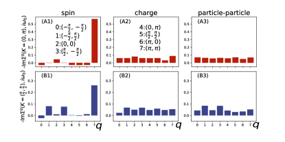
Figure S12: Comparison of $\mathrm{Im}\Sigma^{\mathbf{q}}_{sp/ch/pp}(\mathbf{k},i\omega_{0})$ at $U=7t,t^{\prime}=-0.2,p=0.18$ in three different channels: spin, charge, particle-particle. A1-A3: For the antinode, $\mathbf{k}=(0,\pi)$. B1-B3: For the node, $\mathbf{k}=(\pi/2,\pi/2)$.

Appendix J Fluctuation analysis of the self-energy at large dopings in the NFL

In the main text, we have shown $-\mathrm{Im}\Sigma^{\mathbf{q}/\Omega_{n}}_{sp}(\mathbf{k},i\omega_{0})$ for $p=0.18$ and $p=0.20$ in the NFL. In the following figure, we present the DSEOM decomposition in the spin channel for more NFL doping levels.

As we can see in Fig. S13, for $p=0.24$ and $p=0.26$ at the antinode, $\mathbf{k}=(0,\pi)$, the AFM $\mathbf{q}=(\pi,\pi)$ fluctuations always have by far the largest contribution to $-\mathrm{Im}\Sigma(\mathbf{k},i\omega_{0})$. For the node, $\mathbf{k}=(\pi/2,\pi/2)$, the $\mathbf{q}=(\pi,\pi)$ mode contribution is still the largest, but there are also $\mathbf{q}=(\frac{-\pi}{2},\frac{\pi}{2})$, $(\frac{\pi}{2},\frac{-\pi}{2})$ modes that lead to significant sources of scatterings. Looking carefully, for the node $\mathbf{k}=(\frac{\pi}{2},\frac{\pi}{2})$, scatterings from these two magnetic modes actually involve $(0,\pi)$/$(\pi,0)$ momenta in the Dyson Schwinger equation [since $\mathbf{k}+\mathbf{q}$=$(0,\pi)$/$(\pi,0)$ for $\mathbf{q}=(\frac{-\pi}{2},\frac{\pi}{2})$, $(\frac{\pi}{2},\frac{-\pi}{2})$ respectively]. Since $(0,\pi)$,$(\pi,0)$ are van Hove singularities (VHS), flatband effects can increase scattering phase space. So we argue that nodal electrons in the NFL can be scattered relatively more frequently by non-($\pi,\pi$) modes, given also that $(\pi,\pi)$ antiferromagntic correlations are suppressed by doping. (Note that for the antinode $\mathbf{k}=(0,\pi)$ or $\mathbf{k}=(\pi,0)$, the $\mathbf{q}=(\pi,\pi)$ mode always scatters electrons between VHS, since $\mathbf{k},\mathbf{k}+\mathbf{q}$ are both VHS).

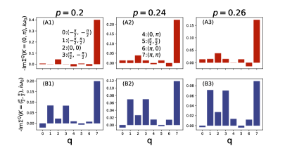
Figure S13: Comparison of $\mathrm{Im}\Sigma^{\mathbf{q}}_{sp/ch/pp}(\mathbf{k},i\omega_{0})$ at $U=7t,t^{\prime}=-0.2,p=0.18$ in the spin channel, for three different dopings A1-A3: For the antinode, $\mathbf{k}=(0,\pi)$. B1-B3: For the node, $\mathbf{k}=(\pi/2,\pi/2)$.

Appendix K DCA cluster size effect: Four-site and sixteen-site results

Here we show results from larger $4\times 4$ DCA cluster computations. Owing to the minus sign problem of the impurity solver, we are not able to do calculations at temperatures $T$ as low as those for the 8-site cluster. As shown in Fig. S14 we are still able to obtain a $T-$ linear scattering rate up to relatively low-temperatures, namely $T/t\sim 0.1$ (at $p=0.05,0.08$ in the underdoped regime, when $T^{*}$ is not yet reached). The fluctuation analysis in the $T-$ linear regime also suggests that the AFM fluctuations $\mathbf{q}=(\pi,\pi)$ are the main source of $T-$ linear electronic scattering rate, as shown in Fig. S14. For a smaller $2\times 2$ cluster we obtained the same results (not shown here).

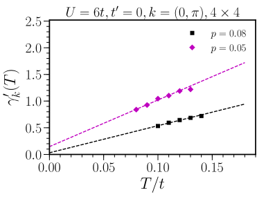
Figure S14: Antinodal scattering rate $\gamma^{\prime}_{k}(T)$, $\mathbf{k}=(0,\pi)$ as a function of temperature $T$ at two dopings for $4\times 4$ DCA cluster.

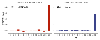
Figure S15: Dyson-Schwinger equation of motion decomposition of the self-energy in the spin channel, $\mathrm{Im}\Sigma^{\mathbf{q}}_{sp}(\mathbf{k},i\omega_{0})$ for the $4\times 4$ DCA cluster. The $\mathbf{q}$ indices are, 0:$(-\frac{\pi}{2},-\frac{\pi}{2})$ 1:$(-\frac{\pi}{2},0)$ 2:$(-\frac{\pi}{2},\frac{\pi}{2})$ 3:$(-\frac{\pi}{2},\pi)$ 4:$(0,-\frac{\pi}{2})$ 5:$(0,0)$ 6:$(0,\frac{\pi}{2})$ 7:$(0,\pi)$ 8:$(\frac{\pi}{2},-\frac{\pi}{2})$ 9:$(\frac{\pi}{2},0)$ 10:$(\frac{\pi}{2},\frac{\pi}{2})$ 11:$(\frac{\pi}{2},\pi)$ 12:$(\pi,-\frac{\pi}{2})$ 13:$(\pi,0)$ 14:$(\pi,\frac{\pi}{2})$ 15:$(\pi,\pi)$.

Appendix L On the nearly Planckian liquid

We focused on the so-called strange metal, that refers to the regime where a linear temperature dependence of the scattering rate extends all the way to zero temperature. The case where the coefficient $C$ of the scattering rate $CT$ is equal to unity (in units $k_{B}=1$, $\hbar=1$) is conjectured in the literature to be a fundamental limit, the “Planckian limit”Bruin et al. (2013); Zaanen et al. (2019); Legros et al. (2019); Grissonnanche et al. (2021); Hartnoll and Mackenzie (2021).

A linear in $T$ scattering rate follows, for example, in the case of phonon scattering when $T$ is larger than the Debye frequency, because then the number of bosonic scatterers is proportional to $T$ Sadovskii (2021). A similar idea has been proposed in the case of an antiferromagnetic QCPMillis (1993); Gegenwart et al. (2008); Löhneysen et al. (2007); Xu et al. (2020); Dumitrescu et al. (2021) because at the QCP the characteristic spin fluctuation frequency, that plays a role analog to the Debye frequency, vanishes. The latter explanation does not hold in the weak correlation limit for two reasons. First, the QCP occurs at an isolated doping and, second, one expects that scattering will be strong only at hot spots on the Fermi surface so that the scattering rate will not be isotropic and, barring disorder effects Rosch (1999), the resulting resistivity will be short-circuited by Fermi-liquid-like portions of the Fermi surface Hlubina and Rice (1995).

The strong to intermediate correlation limit that we have considered here seems to solve the above two problems. First, the linear $T$ NFL regime holds in a finite range of overdoping, as observed experimentally Cooper et al. (2009). Of course, here we should leave open the possibility that the finite intercept found for the antinodal scattering rate could be a signature of finite crossover temperatures ($T^{*}$ or $T_{FL}$) that are too small to be accessible numerically ($<0.025t$) . Clearly, however, our calculations strongly suggest that the extrapolated crossover temperatures are very small if not vanishing (see Fig. S7).

Second, for the strong interaction, $U=7t$, that we considered, it is quite possible that the lack of well-defined quasiparticles leads to spin fluctuations with vanishing characteristic frequency. Then, the argument that the number of scatterers scales like $T$ should hold. Moreover, in over-doped regime the correlation length is small Kastner et al. (1998) so that the spin fluctuations can scatter effectively electrons at all the remains of the Fermi surface. Hence, the argument that the T-linear scattering rate is isotropic will also hold. The only question left then, is why is the coefficient close to unity for many materials. We offer the following explanation. On dimensional grounds, we can write, (restoring physical units)

$$-\mathrm{Im}\Sigma(T)=k_{B}T\times f(\frac{k_{B}T}{\hbar\omega^{*}},\frac{U_{e}}{W})$$ (S24)

where $f$ is a dimensionless scaling function while $\hbar\omega^{*}$ is the characteristic spin-fluctuation energy, $W$ the bandwidth and $U_{e}$ the screened interaction. When $\hbar\omega^{*}$ is large, a Taylor expansion of the scaling function in terms of its first argument gives the Fermi liquid result that the scattering rate is proportional to $(k_{B}T)^{2}$. Following the argument of Kanamori Kanamori (1963) and Brückner Brueckner et al. (1960), the bare interaction $U$ is screened by quantum fluctuations and the resulting screened interaction $U_{e}$ becomes nearly equal to the bandwidth $W$ in the dilute limit. Physically, when $U$ is large, the two-particle wave function tends to vanish when two electrons are on the same site. The maximum energy that this can cost is the bandwidth $W$, that becomes the effective interaction energy. While this result can be proven when $U$ is not too large, it is natural to assume that it holds here. In the limit where $\hbar\omega^{*}$ vanishes then, we have

$$-\mathrm{Im}\Sigma(T)=k_{B}T\times f(\infty,a)$$ (S25)

where $a$ is a number of order unity for a wide range of bare $U$, following the Kanamori-Brückner argument. So $-\mathrm{Im}\Sigma(T)$ can take similar values for a wide class of materials whose low-energy behavior is described by a Hubbard model. Since dimensionless functions are usually of order unity, this suggests why the prefactor of $k_{B}T$ is of order unity. But it clearly does not need to be unity. In addition, other dimensionless quantities can appear as additional arguments of this function, such as the ratio $t^{\prime}/t$. In fact, we find a number about equal to three for this function. So we call the strong-interaction case that we studied, a “nearly Planckian liquid” and we argue that Planckian dissipation is not a fundamental limit to the electron scattering rate Sadovskii (2021).

References

- Stewart (2001) G. R. Stewart, Rev. Mod. Phys. 73, 797 (2001).
- Legros et al. (2019) A. Legros, S. Benhabib, W. Tabis, F. Laliberté, M. Dion, M. Lizaire, B. Vignolle, D. Vignolles, H. Raffy, Z. Z. Li, P. Auban-Senzier, N. Doiron-Leyraud, P. Fournier, D. Colson, L. Taillefer, and C. Proust, Nature Physics 15, 142 (2019).
- Zaanen et al. (2019) J. Zaanen et al., SciPost Phys 6, 061 (2019).
- Shen et al. (2020) B. Shen, Y. Zhang, Y. Komijani, M. Nicklas, R. Borth, A. Wang, Y. Chen, Z. Nie, R. Li, X. Lu, H. Lee, M. Smidman, F. Steglich, P. Coleman, and H. Yuan, Nature 579, 51 (2020).
- Varma (2020) C. M. Varma, Rev. Mod. Phys. 92, 031001 (2020).
- Hartnoll and Mackenzie (2021) S. A. Hartnoll and A. P. Mackenzie, “Planckian dissipation in metals,” (2021), arXiv:2107.07802 [cond-mat.str-el] .
- Ayres et al. (2021) J. Ayres, M. Berben, M. Čulo, Y.-T. Hsu, E. van Heumen, Y. Huang, J. Zaanen, T. Kondo, T. Takeuchi, J. R. Cooper, and et al., Nature 595, 661–666 (2021).
- Cooper et al. (2009) R. A. Cooper, Y. Wang, B. Vignolle, O. J. Lipscombe, S. M. Hayden, Y. Tanabe, T. Adachi, Y. Koike, M. Nohara, H. Takagi, C. Proust, and N. E. Hussey, Science 323, 603 (2009), https://science.sciencemag.org/content/323/5914/603.full.pdf .
- Daou et al. (2009) R. Daou, N. Doiron-Leyraud, D. LeBoeuf, S. Y. Li, F. Laliberté, O. Cyr-Choinière, Y. J. Jo, L. Balicas, J.-Q. Yan, J.-S. Zhou, J. B. Goodenough, and L. Taillefer, Nature Physics 5, 31 (2009).
- Hussey et al. (2011) N. E. Hussey, R. A. Cooper, X. Xu, Y. Wang, I. Mouzopoulou, B. Vignolle, and C. Proust, Philosophical Transactions of the Royal Society A: Mathematical, Physical and Engineering Sciences 369, 1626 (2011), https://royalsocietypublishing.org/doi/pdf/10.1098/rsta.2010.0196 .
- Löhneysen et al. (1994) H. v. Löhneysen, T. Pietrus, G. Portisch, H. G. Schlager, A. Schröder, M. Sieck, and T. Trappmann, Phys. Rev. Lett. 72, 3262 (1994).
- Grigera et al. (2001) S. A. Grigera, R. S. Perry, A. J. Schofield, M. Chiao, S. R. Julian, G. G. Lonzarich, S. I. Ikeda, Y. Maeno, A. J. Millis, and A. P. Mackenzie, Science 294, 329 (2001), https://science.sciencemag.org/content/294/5541/329.full.pdf .
- Doiron-Leyraud et al. (2009) N. Doiron-Leyraud, P. Auban-Senzier, S. René de Cotret, C. Bourbonnais, D. Jérome, K. Bechgaard, and L. Taillefer, Phys. Rev. B 80, 214531 (2009).
- Varma et al. (1989) C. M. Varma, P. B. Littlewood, S. Schmitt-Rink, E. Abrahams, and A. E. Ruckenstein, Phys. Rev. Lett. 63, 1996 (1989).
- Rice et al. (2017) T. M. Rice, N. J. Robinson, and A. M. Tsvelik, Phys. Rev. B 96, 220502 (2017).
- Millis (1993) A. J. Millis, Phys. Rev. B 48, 7183 (1993).
- Abanov et al. (2003) A. Abanov, A. V. Chubukov, and J. Schmalian, Advances in Physics 52, 119 (2003).
- Gegenwart et al. (2008) P. Gegenwart, Q. Si, and F. Steglich, Nature Physics 4, 186 (2008).
- Löhneysen et al. (2007) H. v. Löhneysen, A. Rosch, M. Vojta, and P. Wölfle, Rev. Mod. Phys. 79, 1015 (2007).
- Xu et al. (2020) X. Y. Xu, A. Klein, K. Sun, A. V. Chubukov, and Z. Y. Meng, npj Quantum Materials 5, 65 (2020).
- Dumitrescu et al. (2021) P. T. Dumitrescu, N. Wentzell, A. Georges, and O. Parcollet, arXiv preprint arXiv:2103.08607 (2021).
- Cha et al. (2020a) P. Cha, N. Wentzell, O. Parcollet, A. Georges, and E.-A. Kim, Proceedings of the National Academy of Sciences 117, 18341 (2020a), https://www.pnas.org/content/117/31/18341.full.pdf .
- Sachdev and Ye (1993) S. Sachdev and J. Ye, Phys. Rev. Lett. 70, 3339 (1993).
- Patel and Sachdev (2019) A. A. Patel and S. Sachdev, Phys. Rev. Lett. 123, 066601 (2019).
- Parcollet and Georges (1999) O. Parcollet and A. Georges, Physical Review B 59, 5341 (1999).
- Scalapino (2007) D. J. Scalapino, in Handbook of High-Temperature Superconductivity: Theory and Experiment, edited by J. R. Schrieffer and J. S. Brooks (Springer New York, 2007) pp. 495–526.
- Maier et al. (2005a) T. A. Maier, M. Jarrell, T. C. Schulthess, P. R. C. Kent, and J. B. White, Physical Review Letters 95, 237001 (2005a).
- Gull et al. (2013) E. Gull, O. Parcollet, and A. J. Millis, Physical Review Letters 110, 216405 (2013).
- Fratino et al. (2016) L. Fratino, P. Sémon, G. Sordi, and A.-M. Tremblay, Scientific reports 6, 22715 (2016).
- Macridin et al. (2006) A. Macridin, M. Jarrell, T. Maier, P. R. C. Kent, and E. D’Azevedo, Phys. Rev. Lett. 97, 036401 (2006).
- Sénéchal and Tremblay (2004) D. Sénéchal and A.-M. S. Tremblay, Phys. Rev. Lett. 92, 126401 (2004).
- Sordi et al. (2012) G. Sordi, P. Sémon, K. Haule, and A.-M. S. Tremblay, Scientific Reports 2 (2012), 10.1038/srep00547.
- Wu et al. (2018) W. Wu, M. S. Scheurer, S. Chatterjee, S. Sachdev, A. Georges, and M. Ferrero, Phys. Rev. X 8, 021048 (2018).
- Reymbaut et al. (2019) A. Reymbaut, S. Bergeron, R. Garioud, M. Thénault, M. Charlebois, P. Sémon, and A.-M. S. Tremblay, Phys. Rev. Research 1, 023015 (2019).
- Zheng et al. (2017) B.-X. Zheng, C.-M. Chung, P. Corboz, G. Ehlers, M.-P. Qin, R. M. Noack, H. Shi, S. R. White, S. Zhang, and G. K.-L. Chan, Science 358, 1155 (2017), https://science.sciencemag.org/content/358/6367/1155.full.pdf .
- Dash and Sénéchal (2020) S. S. Dash and D. Sénéchal, arXiv:2008.08661 [cond-mat] (2020), arXiv: 2008.08661.
- Perepelitsky et al. (2016) E. Perepelitsky, A. Galatas, J. Mravlje, R. Žitko, E. Khatami, B. S. Shastry, and A. Georges, Phys. Rev. B 94, 235115 (2016).
- Huang et al. (2019) E. W. Huang, R. Sheppard, B. Moritz, and T. P. Devereaux, Science 366, 987 (2019).
- Cha et al. (2020b) P. Cha, A. A. Patel, E. Gull, and E.-A. Kim, Phys. Rev. Research 2, 033434 (2020b).
- Brown et al. (2018) P. T. Brown, D. Mitra, E. Guardado-Sanchez, R. Nourafkan, A. Reymbaut, C.-D. Hébert, S. Bergeron, A.-M. S. Tremblay, J. Kokalj, D. A. Huse, and et al., Science (2018), 10.1126/science.aat4134.
- Gunnarsson et al. (2003) O. Gunnarsson, M. Calandra, and J. E. Han, Rev. Mod. Phys. 75, 1085 (2003).
- Grissonnanche et al. (2021) G. Grissonnanche, Y. Fang, A. Legros, S. Verret, F. Laliberté, C. Collignon, J. Zhou, D. Graf, P. A. Goddard, L. Taillefer, et al., Nature 595, 667 (2021).
- Maier et al. (2005b) T. Maier, M. Jarrell, T. Pruschke, and M. H. Hettler, Rev. Mod. Phys. 77, 1027 (2005b).
- Chen et al. (2019) S.-D. Chen, M. Hashimoto, Y. He, D. Song, K.-J. Xu, J.-F. He, T. P. Devereaux, H. Eisaki, D.-H. Lu, J. Zaanen, and Z.-X. Shen, Science 366, 1099 (2019), https://science.sciencemag.org/content/366/6469/1099.full.pdf .
- Pavarini et al. (2001) E. Pavarini, I. Dasgupta, T. Saha-Dasgupta, O. Jepsen, and O. K. Andersen, Phys. Rev. Lett. 87, 047003 (2001).
- Georges et al. (1996) A. Georges, G. Kotliar, W. Krauth, and M. J. Rozenberg, Rev. Mod. Phys. 68, 13 (1996).
- Barišić et al. (2013) N. Barišić, M. K. Chan, Y. Li, G. Yu, X. Zhao, M. Dressel, A. Smontara, and M. Greven, Proceedings of the National Academy of Sciences 110, 12235 (2013), https://www.pnas.org/content/110/30/12235.full.pdf .
- Schröder et al. (2000) A. Schröder, G. Aeppli, R. Coldea, M. Adams, O. Stockert, H. Löhneysen, E. Bucher, R. Ramazashvili, and P. Coleman, Nature 407, 351 (2000).
- Schäfer et al. (2021) T. Schäfer, N. Wentzell, F. Šimkovic, Y.-Y. He, C. Hille, M. Klett, C. J. Eckhardt, B. Arzhang, V. Harkov, F. m. c.-M. Le Régent, A. Kirsch, Y. Wang, A. J. Kim, E. Kozik, E. A. Stepanov, A. Kauch, S. Andergassen, P. Hansmann, D. Rohe, Y. M. Vilk, J. P. F. LeBlanc, S. Zhang, A.-M. S. Tremblay, M. Ferrero, O. Parcollet, and A. Georges, Phys. Rev. X 11, 011058 (2021).
- Cyr-Choinière et al. (2018) O. Cyr-Choinière, R. Daou, F. Laliberté, C. Collignon, S. Badoux, D. LeBoeuf, J. Chang, B. J. Ramshaw, D. A. Bonn, W. N. Hardy, R. Liang, J.-Q. Yan, J.-G. Cheng, J.-S. Zhou, J. B. Goodenough, S. Pyon, T. Takayama, H. Takagi, N. Doiron-Leyraud, and L. Taillefer, Phys. Rev. B 97, 064502 (2018).
- Gull et al. (2010) E. Gull, M. Ferrero, O. Parcollet, A. Georges, and A. J. Millis, Phys. Rev. B 82, 155101 (2010).
- Sordi et al. (2013) G. Sordi, P. Sémon, K. Haule, and A.-M. S. Tremblay, Phys. Rev. B 87, 041101 (2013).
- Xu et al. (2013) W. Xu, K. Haule, and G. Kotliar, Physical review letters 111, 036401 (2013).
- Gunnarsson et al. (2015) O. Gunnarsson, T. Schäfer, J. P. F. LeBlanc, E. Gull, J. Merino, G. Sangiovanni, G. Rohringer, and A. Toschi, Phys. Rev. Lett. 114, 236402 (2015).
- Wu et al. (2017) W. Wu, M. Ferrero, A. Georges, and E. Kozik, Phys. Rev. B 96, 041105(R) (2017).
- Wakimoto et al. (2007) S. Wakimoto, K. Yamada, J. M. Tranquada, C. D. Frost, R. J. Birgeneau, and H. Zhang, Phys. Rev. Lett. 98, 247003 (2007).
- Le Tacon et al. (2013) M. Le Tacon, M. Minola, D. C. Peets, M. Moretti Sala, S. Blanco-Canosa, V. Hinkov, R. Liang, D. A. Bonn, W. N. Hardy, C. T. Lin, and et al., Physical Review B 88, 020501 (2013).
- Kaminski et al. (2005) A. Kaminski, H. M. Fretwell, M. R. Norman, M. Randeria, S. Rosenkranz, U. Chatterjee, J. C. Campuzano, J. Mesot, T. Sato, T. Takahashi, and et al., Physical Review B 71, 014517 (2005).
- Sadovskii (2021) M. V. Sadovskii, Physics-Uspekhi 64, 175 (2021).
- Rosch (1999) A. Rosch, Phys. Rev. Lett. 82, 4280 (1999).
- Hlubina and Rice (1995) R. Hlubina and T. M. Rice, Phys. Rev. B 51, 9253 (1995).
- Kastner et al. (1998) M. A. Kastner, R. J. Birgeneau, G. Shirane, and Y. Endoh, Rev. Mod. Phys. 70, 897 (1998).
- Nicholas et al. (2021) R. P. Nicholas, S. Tarapada, P. L. Ricardo, D. S. Sankar, and R. L. Greene, arXiv preprint arXiv:2109.00513 (2021).
- Hirsch and Fye (1986) J. E. Hirsch and R. M. Fye, Physical review letters 56, 2521 (1986).
- Gull et al. (2011) E. Gull, A. J. Millis, A. I. Lichtenstein, A. N. Rubtsov, M. Troyer, and P. Werner, Rev. Mod. Phys. 83, 349 (2011).
- Sachdev (2011) S. Sachdev, Quantum Phase Transitions, 2nd ed. (Cambridge University Press, 2011).
- Bergeron and Tremblay (2016) D. Bergeron and A.-M. S. Tremblay, Phys. Rev. E 94, 023303 (2016).
- Bruin et al. (2013) J. a. N. Bruin, H. Sakai, R. S. Perry, and A. P. Mackenzie, Science 339, 804–807 (2013).
- Wu et al. (2020) W. Wu, M. S. Scheurer, M. Ferrero, and A. Georges, Phys. Rev. Research 2, 033067 (2020).
- Kanamori (1963) J. Kanamori, Progress of Theoretical Physics 30, 275 (1963).
- Brueckner et al. (1960) K. A. Brueckner, T. Soda, P. W. Anderson, and P. Morel, Phys. Rev. 118, 1442 (1960).