A Method for Inferring Polymers Based on Linear Regression and Integer Programming

Ryota Ido¹, Shengjuan Cao¹, Jianshen Zhu¹, Naveed Ahmed Azam¹, Kazuya Haraguchi¹, Liang Zhao², Hiroshi Nagamochi¹ and Tatsuya Akutsu³

¹Department of Applied Mathematics and Physics, Kyoto University, Kyoto 606-8501, Japan
²Graduate School of Advanced Integrated Studies in Human Survavibility (Shishu-Kan), Kyoto University, Kyoto 606-8306, Japan
³Bioinformatics Center, Institute for Chemical Research, Kyoto University, Uji 611-0011, Japan

Abstract
A novel framework has recently been proposed for designing the molecular structure of chemical compounds with a desired chemical property using both artificial neural networks and mixed integer linear programming. In this paper, we design a new method for inferring a polymer based on the framework. For this, we introduce a new way of representing a polymer as a form of monomer and define new descriptors that feature the structure of polymers. We also use linear regression as a building block of constructing a prediction function in the framework. The results of our computational experiments reveal a set of chemical properties on polymers to which a prediction function constructed with linear regression performs well. We also observe that the proposed method can infer polymers with up to 50 non-hydrogen atoms in a monomer form.

Keywords: Machine Learning, Linear Regression, Integer Programming, Polymers, Cheminformatics, Materials Informatics, QSAR/QSPR, Molecular Design.

1 Introduction

Background  In recent years, molecular design has received a great deal of attention from various research fields such as chemoinformatics, bioinformatics, and materials informatics [1, 2, 3]. In particular, extensive studies have been done for molecular design using artificial neural networks (ANNs). Various ANN models have been applied in these studies, which include recurrent neural networks [4, 5], variational autoencoders [6], grammar variational autoencoders [7], generative adversarial networks [8, 9], and invertible flow models [10, 11]. Many of these studies employ graph convolution techniques [12] to effectively handle molecules represented as chemical graphs.

Molecular design has also been studied for many years in chemoinformatics, under the name of inverse quantitative structure activity relationship (inverse QSAR). The purpose of this framework is to seek for chemical structures having desired chemical activities under some constraints, where the task of prediction of chemical activities from their chemical structures is referred to as QSAR (or, forward QSAR). In both forward and inverse QSAR, chemical structures are represented as undirected graphs (chemical graphs). Then, chemical graphs are transformed into vectors of real or integer numbers, which are called descriptors in chemoinformatics and vectors correspond to feature vectors in machine learning. One of the typical approaches to inverse QSAR is to infer feature vectors from given chemical activities and constraints and then reconstruct chemical graphs from these feature vectors [13, 14, 15]. However, the reconstruction itself is a challenging task because it is known to be NP-hard (i.e., theoretically intractable) [16]. Such a difficulty is also suggested from a huge size of chemical graph space. For example, the number of chemical graphs with up to 30 atoms (vertices) C, N, O, and S may exceed $10^{60}$ [17]. Due to this inherent difficulty, most methods for inverse QSAR, including recent ANN-based ones, do not guarantee optimal or exact solutions.

The targets of most of the inverse QSAR methods and ANN-based molecular design methods had been small chemical compounds. On the other hand, it is known that macromolecules, especially polymers, have also a wide range of applications in both medical science and material science [18, 19]. Accordingly, several studies have recently been done on computational design of polymers [20, 21]. However, it was pointed out that very few studies addressed the representation of polymer structures [22], and thus the development of novel and useful representation methods for polymers remains a challenge.

Figure 1: An illustration of a framework for inferring a set of chemical graphs $\mathbb{C}^{*}$.

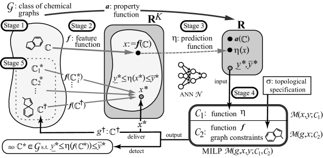
Framework  Akutsu and Nagamochi [23] proved that the computation process of a given ANN can be simulated with a mixed integer linear programming (MILP). Based on this, a novel framework for inferring chemical graphs has been developed and revised [24, 25, 26], as illustrated in Figure 1. It constructs a prediction function in the first phase and infers a chemical graph in the second phase. The first phase of the framework consists of three stages. In Stage 1, we choose a chemical property $\pi$ and a class $\mathcal{G}$ of graphs, where a property function $a$ is defined so that $a(\mathbb{C})$ is the value of $\pi$ for a compound $\mathbb{C}\in\mathcal{G}$, and collect a data set $D_{\pi}$ of chemical graphs in $\mathcal{G}$ such that $a(\mathbb{C})$ is available for every $\mathbb{C}\in D_{\pi}$. In Stage 2, we introduce a feature function $f:\mathcal{G}\to\mathbb{R}^{K}$ for a positive integer $K$. In Stage 3, we construct a prediction function $\eta$ with an ANN $\mathcal{N}$ that, given a vector $x\in\mathbb{R}^{K}$, returns a value $y=\eta(x)\in\mathbb{R}$ so that $\eta(f(\mathbb{C}))$ serves as a predicted value to the real value $a(\mathbb{C})$ of $\pi$ for each $\mathbb{C}\in D_{\pi}$. Given two reals $\underline{y}^{*}$ and $\overline{y}^{*}$ as an interval for a target chemical value, the second phase infers chemical graphs $\mathbb{C}^{*}$ with $\underline{y}^{*}\leq\eta(f(\mathbb{C}^{*}))\leq\overline{y}^{*}$ in the next two stages. We have obtained a feature function $f$ and a prediction function $\eta$ and call an additional constraint on the substructures of target chemical graphs a topological specification. In Stage 4, we prepare the following two MILP formulations:

1. MILP $\mathcal{M}(x,y;\mathcal{C}_{1})$ with a set $\mathcal{C}_{1}$ of linear constraints on variables $x$ and $y$ (and some other auxiliary variables) simulates the process of computing $y:=\eta(x)$ from a vector $x$; and

2. MILP $\mathcal{M}(g,x;\mathcal{C}_{2})$ with a set $\mathcal{C}_{2}$ of linear constraints on variable $x$ and a variable vector $g$ that represents a chemical graph $\mathbb{C}$ (and some other auxiliary variables) simulates the process of computing $x:=f(\mathbb{C})$ from a chemical graph $\mathbb{C}$ and chooses a chemical graph $\mathbb{C}$ that satisfies the given topological specification $\sigma$.

Given an interval with $\underline{y}^{*},\overline{y}^{*}\in\mathbb{R}$, we solve the combined MILP $\mathcal{M}(g,x,y;\mathcal{C}_{1},\mathcal{C}_{2})$ to find a feature vector $x^{*}\in\mathbb{R}^{K}$ and a chemical graph $\mathbb{C}^{\dagger}$ with the specification $\sigma$ such that $f(\mathbb{C}^{\dagger})=x^{*}$ and $\underline{y}^{*}\leq\eta(x^{*})\leq\overline{y}^{*}$ (where if the MILP instance is infeasible then this suggests that there does not exist such a desired chemical graph). In Stage 5, we generate other chemical graphs $\mathbb{C}^{*}$ such that $\underline{y}^{*}\leq\eta(f(\mathbb{C}^{*}))\leq\overline{y}^{*}$ based on the output chemical graph $\mathbb{C}^{\dagger}$.

MILP formulations required in Stage 4 have been designed for chemical compounds with cycle index 0 (i.e., acyclic) [25, 27], cycle index 1 [28] and cycle index 2 [29], where no sophisticated topological specification was available yet. Azam et al. [27] introduced a restricted class of acyclic graphs that is characterized by an integer ${\rho}$, called a “branch-parameter” such that the restricted class still covers most of the acyclic chemical compounds in the database. Akutsu and Nagamochi [30] extended the idea to define a restricted class of cyclic graphs, called “${\rho}$-lean cyclic graphs” and introduced a set of flexible rules for describing a topological specification. Recently, Tanaka et al. [31] (resp., Zhu et al. [26]) used a decision tree (resp., linear regression) to construct a prediction function $\eta$ in Stage 3 in the framework and derived an MILP $\mathcal{M}(x,y;\mathcal{C}_{1})$ that simulates the computation process of a decision tree (resp., linear regression).

Two-layered Model  Shi et al. [32] proposed a method, called a two-layered model for representing the feature of a chemical graph in order to deal with an arbitrary graph in the framework. In the two-layered model, a chemical graph $\mathbb{C}$ with a parameter ${\rho}\geq 1$ is regarded as two parts: the exterior and the interior of the hydrogen-suppressed chemical graph $\langle\mathbb{C}\rangle$ obtained from $\mathbb{C}$ by removing hydrogen. The exterior consists of maximal acyclic induced subgraphs with height at most ${\rho}$ in $\langle\mathbb{C}\rangle$ and the interior is the connected subgraph of $\langle\mathbb{C}\rangle$ obtained by ignoring the exterior. Shi et al. [32] defined a feature vector $f(\mathbb{C})$ of a chemical graph $\mathbb{C}$ to be a combination of the frequency of adjacent atom pairs in the interior and the frequency of chemical acyclic graphs among the set of chemical rooted trees $T_{u}$ rooted at interior-vertices $u$. Tanaka et al. [31] constructed a prediction function with a decision tree by using the feature vector by Shi et al. [32]. Recently, Zhu et al. [26] extended the model to treat chemical elements of multiple valence and chemical compounds with cations and anions.

Contribution  In order to extend our MILP-based framework for designing novel polymers, we modify the method due to Zhu et al. [26]. For this, we introduce a new way of representing a polymer as a form of monomer and define new descriptors that feature the structure of polymers. We modify the MILP formulation proposed by Zhu et al. [26] due to the change of feature function $f$ (the detail of the MILP $\mathcal{M}(g,x;\mathcal{C}_{2})$ can be found in Appendix E). To generate target chemical graphs $\mathbb{C}^{*}$ in Stage 5, we also use and modify the dynamic programming algorithm due to Zhu et al. [26].

We implemented the framework based on the refined two-layered model and a prediction function by linear regression. A polymer was inferred by using the framework for the first time in this paper, where Tanaka et al. [31] studied constructing a prediction function with a decision tree for some polymer properties but have not argued topological specification of polymers and inference of a polymer. The results of our computational experiments reveal a set of chemical properties on polymers to which a prediction function constructed with linear regression on our feature function performs well. We also observe that the proposed method can infer a polymer with up to 50 non-hydrogen atoms in a monomer form.

The paper is organized as follows. Section 2 introduces some notions on graphs, a modeling of chemical compounds and define a new monomer representation of polymers. Section 3 describes the two-layered model for polymers. Section 4 reports the results on some computational experiments conducted for eight chemical properties on polymers such as glass transition and experimental amorphous density. Section 5 makes some concluding remarks.

Some technical details are given in Appendices: Appendix A for the idea of linear regression and an MILP $\mathcal{M}(x,y;\mathcal{C}_{1})$ formulated by Zhu et al. [26] that simulates a process of computing a prediction function constructed by linear regression; Appendix B for all descriptors in our feature function on polymers; Appendix C for a full description of a topological specification; Appendix D for the detail of test instances used in our computational experiment for Stages 4 and 5; and Appendix E for the details of our MILP formulation $\mathcal{M}(g,x;\mathcal{C}_{2})$. Note that the modification of the dynamic programming algorithm is not given in Appendices because it is slight and straightforward.

2 Preliminary

This section introduces some notions and terminologies on graphs, modeling of chemical compounds and our choice of descriptors.

Let $\mathbb{R}$, $\mathbb{Z}$ and $\mathbb{Z}_{+}$ denote the sets of reals, integers and non-negative integers, respectively. For two integers $a$ and $b$, let $[a,b]$ denote the set of integers $i$ with $a\leq i\leq b$.

Graph Given a graph $G$, let $V(G)$ and $E(G)$ denote the sets of vertices and edges, respectively. For a subset $V^{\prime}\subseteq V(G)$ (resp., $E^{\prime}\subseteq E(G))$ of a graph $G$, let $G-V^{\prime}$ (resp., $G-E^{\prime}$) denote the graph obtained from $G$ by removing the vertices in $V^{\prime}$ (resp., the edges in $E^{\prime}$), where we remove all edges incident to a vertex in $V^{\prime}$ in $G-V^{\prime}$. An edge subset $E^{\prime}\subseteq E(G)$ in a connected graph $G$ is called separating (resp., non-separating) if $G-E^{\prime}$ becomes disconnected (resp., $G-E^{\prime}$ remains connected). The rank $\mathrm{r}(G)$ of a graph $G$ is defined to be the minimum $|F|$ of an edge subset $F\subseteq E(G)$ such that $G-F$ contains no cycle, where $\mathrm{r}(G)=|E(G)|-|V(G)|+1$ for a connected graph $G$. Observe that $\mathrm{r}(G-E^{\prime})=\mathrm{r}(G)-|E^{\prime}|$ holds for any non-separating edge subset $E^{\prime}\subseteq E(G)$. An edge $e\in E(G)$ in a connected graph $G$ is called a bridge if $\{e\}$ is separating. For a connected cyclic graph $G$, an edge $e$ is called a core-edge if it is in a cycle of $G$ or is a bridge $e=u_{1}u_{2}$ such that each of the connected graphs $G_{i}$, $i=1,2$ of $G-e$ contains a cycle. A vertex incident to a core-edge is called a core-vertex of $G$. A path with two end-vertices $u$ and $v$ is called a $u,v$-path. A set $F$ of edges in $G$ is called a circular set if $G$ contains a cycle $C$ that contains all edges in $F$ and for every edge $e\in F$, $F\setminus\{e\}$ is the set of all bridges $e^{\prime}\in F$ in the graph $G-e$.

We define a rooted graph to be a graph with a designated vertex, called a root. For a graph $G$ possibly with a root, a leaf-vertex is defined to be a non-root vertex with degree 1. We call the edge $uv$ incident to a leaf vertex $v$ a leaf-edge, and denote by $V_{\mathrm{leaf}}(G)$ and $E_{\mathrm{leaf}}(G)$ the sets of leaf-vertices and leaf-edges in $G$, respectively. For a graph or a rooted graph $G$, we define graphs $G_{i},i\in\mathbb{Z}_{+}$ obtained from $G$ by removing the set of leaf-vertices $i$ times so that

$$G_{0}:=G;~{}~{}G_{i+1}:=G_{i}-V_{\mathrm{leaf}}(G_{i}),$$

where we call a vertex $v$ a tree vertex if $v\in V_{\mathrm{leaf}}(G_{i})$ for some $i\geq 0$. Define the height $\mathrm{ht}(v)$ of each tree vertex $v\in V_{\mathrm{leaf}}(G_{i})$ to be $i$; and $\mathrm{ht}(v)$ of each non-tree vertex $v$ adjacent to a tree vertex to be $\mathrm{ht}(u)+1$ for the maximum $\mathrm{ht}(u)$ of a tree vertex $u$ adjacent to $v$, where we do not define height of any non-tree vertex not adjacent to any tree vertex. We call a vertex $v$ with $\mathrm{ht}(v)=k$ a leaf $k$-branch. The height $\mathrm{ht}(T)$ of a rooted tree $T$ is defined to be the maximum of $\mathrm{ht}(v)$ of a vertex $v\in V(T)$. For an integer $k\geq 0$, we call a rooted tree $T$ $k$-lean if $T$ has at most one leaf $k$-branch. For an unrooted cyclic graph $G$, we regard that the set of non-core-edges in $G$ induces a collection $\mathcal{T}$ of trees each of which is rooted at a core-vertex, where we call $G$ $k$-lean if each of the rooted trees in $\mathcal{T}$ is $k$-lean.

2.1 Modeling of Chemical Compounds

We review a modeling of chemical compounds (monomers) and introduce a new way of representing a polymer as a form of monomer.

To represent a chemical compound, we introduce a set of chemical elements such as H (hydrogen), C (carbon), O (oxygen), N (nitrogen) and so on. To distinguish a chemical element ${\tt a}$ with multiple valences such as S (sulfur), we denote a chemical element ${\tt a}$ with a valence $i$ by ${\tt a}_{(i)}$, where we do not use such a suffix $(i)$ for a chemical element ${\tt a}$ with a unique valence. Let $\Lambda$ be a set of chemical elements ${\tt a}_{(i)}$. For example, $\Lambda=\{{\tt H},{\tt C},{\tt O},{\tt N},{\tt P},{\tt S}_{(2)},{\tt S}_{(4)},{\tt S}_{(6)}\}$. Let $\mathrm{val}:\Lambda\to[1,6]$ be a valence function. For example, $\mathrm{val}({\tt H})=1$, $\mathrm{val}({\tt C})=4$, $\mathrm{val}({\tt O})=2$, $\mathrm{val}({\tt P})=5$, $\mathrm{val}({\tt S}_{(2)})=2$, $\mathrm{val}({\tt S}_{(4)})=4$ and $\mathrm{val}({\tt S}_{(6)})=6$. For each chemical element ${\tt a}\in\Lambda$, let $\mathrm{mass}({\tt a})$ denote the mass of ${\tt a}$.

A chemical compound is represented by a chemical graph defined to be a tuple $\mathbb{C}=(H,\alpha,\beta)$ of a simple, connected undirected graph $H$ and functions $\alpha:V(H)\to\Lambda$ and $\beta:E(H)\to[1,3]$. The set of atoms and the set of bonds in the compound are represented by the vertex set $V(H)$ and the edge set $E(H)$, respectively. The chemical element assigned to a vertex $v\in V(H)$ is represented by $\alpha(v)$ and the bond-multiplicity between two adjacent vertices $u,v\in V(H)$ is represented by $\beta(e)$ of the edge $e=uv\in E(H)$. We say that two tuples $(H_{i},\alpha_{i},\beta_{i}),i=1,2$ are isomorphic if they admit an isomorphism $\phi$, i.e., a bijection $\phi:V(H_{1})\to V(H_{2})$ such that $uv\in E(H_{1}),\alpha_{1}(u)={\tt a},\alpha_{1}(v)={\tt b},\beta_{1}(uv)=m$ $\leftrightarrow$ $\phi(u)\phi(v)\in E(H_{2}),\alpha_{2}(\phi(u))={\tt a},\alpha_{2}(\phi(v))={\tt b},\beta_{2}(\phi(u)\phi(v))=m$. When $H_{i}$ is rooted at a vertex $r_{i},i=1,2$, $(H_{i},\alpha_{i},\beta_{i}),i=1,2$ are rooted-isomorphic (r-isomorphic) if they admit an isomorphism $\phi$ such that $\phi(r_{1})=r_{2}$.

For a notational convenience, we use a function $\beta_{\mathbb{C}}:V(H)\to[0,12]$ for a chemical graph $\mathbb{C}=(H,\alpha,\beta)$, such that $\beta_{\mathbb{C}}(u)$ means the sum of bond-multiplicities of edges incident to a vertex $u$; i.e.,

$$\beta_{\mathbb{C}}(u)\triangleq\sum_{uv\in E(H)}\beta(uv)\mbox{ for each vertex $u\in V(H)$.}$$

For each vertex $u\in V(H)$, define the electron-degree $\mathrm{eledeg}_{\mathbb{C}}(u)$ to be

$$\mathrm{eledeg}_{\mathbb{C}}(u)\triangleq\beta_{\mathbb{C}}(u)-\mathrm{val}(\alpha(u)).$$

For each vertex $u\in V(H)$, let $\deg_{\mathbb{C}}(v)$ denote the number of vertices adjacent to $u$ in $\mathbb{C}$.

For a chemical graph $\mathbb{C}=(H,\alpha,\beta)$, let $V_{{\tt a}}(\mathbb{C})$, ${\tt a}\in\Lambda$ denote the set of vertices $v\in V(H)$ such that $\alpha(v)={\tt a}$ in $\mathbb{C}$ and define the hydrogen-suppressed chemical graph $\langle\mathbb{C}\rangle$ to be the graph obtained from $H$ by removing all the vertices $v\in V_{\tt H}(\mathbb{C})$.

Figure 2: (a) A repeating unit of polymer: thioBis(4-phenyl)carbonate, where $e^{*}_{0}$ and $e^{*}_{1}$ are the connecting-edges and $v^{*}_{1}$ and $v^{*}_{2}$ are the connecting-vertices; (b) A monomer form of the polymer in (a), where the link-edges are depicted with thick lines and $v^{*}_{1}$ and $v^{*}_{2}$ are the connecting-vertices.

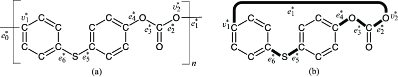
Polymers  In this paper, we treat a polymer that is a linear concatenation of a single repeating unit with two connecting-edges of $e^{*}_{0}$ and $e^{*}_{1}$ such that two adjacent units in the concatenation are joined with the connecting-edges. We call the two vertices incident to the two connecting-edges the connecting-vertices. Figure 2(a) illustrates an example of a repeating unit of such a polymer, where $v^{*}_{1}$ and $v^{*}_{2}$ are the connecting-vertices.

Tanaka et al. [31] proposed a modeling of a polymer as a monomer with no connecting-edges by introducing an artificial chemical element ${\tt a}^{*}$ to which the original two connecting-edges of a repeating unit become newly incident. When the number of repeating units in a polymer is extremely large, other edges in the repeating unit may have a similar role with the connecting-edges. For example, edge $e^{*}_{2}$ of the repeating unit in Figure 2(a) can serve as the connecting-edges of a different repeating unit by splitting $e^{*}_{2}$ into two edges and merging $e^{*}_{0}$ and $e^{*}_{1}$ into a single edge.

To take this into consideration, this paper introduces a new way of representing a polymer as a monomer form. We call an edge $e$ in a repeating unit of a polymer a link-edge if it is passed by every path between the connecting-edges $e^{*}_{0}$ and $e^{*}_{1}$. For example, the link-edges in the repeating unit in Figure 2(a) are given by $e^{*}_{2},e^{*}_{3},\ldots,e^{*}_{6}$. To represent a polymer as a monomer, we regard the two connecting-edges $e^{*}_{0}$ and $e^{*}_{1}$ as a single edge $e^{*}_{1}$, as illustrated in Figure 2(b). We call the resulting chemical graph the monomer representation, where we also call the edge $e^{*}_{1}$ a link-edge in the representation. We still call the vertices incident to $e^{*}_{1}$ the connecting-vertices and distinguish them from other vertices because a polymer that is synthesized from a specified repeating unit actually may end with the connecting-vertices. (A polymer of a cyclic sequence of a repeating unit that has no particular ends can be modeled as our monomer representation with no connecting-vertices.) In what follows, a polymer is represented by the monomer representation $\mathbb{C}$, and the set of link-edges in $\mathbb{C}$ is denoted by $E^{\mathrm{lnk}}(\mathbb{C})$. Note that the set $E^{\mathrm{lnk}}(\mathbb{C})$ is a circular set in $\mathbb{C}$.

3 Two-layered Model

This section reviews the two-layered model proposed by Zhu et al. [26] and makes a necessary modification so as to apply it to the case of polymers.

Let $\mathbb{C}=(H,\alpha,\beta)$ be a chemical graph and ${\rho}\geq 1$ be an integer, which we call a branch-parameter.

A two-layered model of $\mathbb{C}$ is a partition of the hydrogen-suppressed chemical graph $\langle\mathbb{C}\rangle$ into an “interior” and an “exterior” in the following way. We call a vertex $v\in V(\langle\mathbb{C}\rangle)$ (resp., an edge $e\in E(\langle\mathbb{C}\rangle))$ of $\mathbb{C}$ an exterior-vertex (resp., exterior-edge) if $\mathrm{ht}(v)<{\rho}$ (resp., $e$ is incident to an exterior-vertex) and denote the sets of exterior-vertices and exterior-edges by $V^{\mathrm{ex}}(\mathbb{C})$ and $E^{\mathrm{ex}}(\mathbb{C})$, respectively, and denote $V^{\mathrm{int}}(\mathbb{C})=V(\langle\mathbb{C}\rangle)\setminus V^{\mathrm{ex}}(\mathbb{C})$ and $E^{\mathrm{int}}(\mathbb{C})=E(\langle\mathbb{C}\rangle)\setminus E^{\mathrm{ex}}(\mathbb{C})$, respectively. We call a vertex in $V^{\mathrm{int}}(\mathbb{C})$ (resp., an edge in $E^{\mathrm{int}}(\mathbb{C})$) an interior-vertex (resp., interior-edge). The set $E^{\mathrm{ex}}(\mathbb{C})$ of exterior-edges forms a collection of connected graphs each of which is regarded as a rooted tree $T$ rooted at a vertex $v\in V(T)$ with the maximum $\mathrm{ht}(v)$. Let $\mathcal{T}^{\mathrm{ex}}(\langle\mathbb{C}\rangle)$ denote the set of these chemical rooted trees in $\langle\mathbb{C}\rangle$. The interior of $\mathbb{C}$ is defined to be the subgraph $(V^{\mathrm{int}}(\mathbb{C}),E^{\mathrm{int}}(\mathbb{C}))$ of $\langle\mathbb{C}\rangle$.

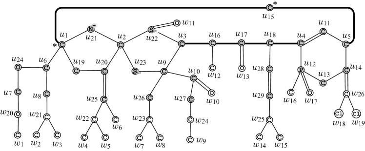
Differently from standard monomers, we distinguish the link-edges in the monomer form of a polymer from other edges in order to feature the topological structure of the polymer. Figure 3 illustrates an example of a hydrogen-suppressed polymer $\langle\mathbb{C}\rangle$ with $E^{\mathrm{lnk}}(\mathbb{C})=\{u_{1}u_{15},$ $u_{5}u_{15},u_{3}u_{16},u_{16}u_{17},u_{17}u_{18},u_{4}u_{18}\}$.

For a branch-parameter ${\rho}=2$, the interior of the chemical graph $\langle\mathbb{C}\rangle$ in Figure 3 is obtained by removing the set of vertices with degree 1 ${\rho}=2$ times; i.e., first remove the set $V_{1}=\{w_{1},w_{2},\ldots,w_{19}\}$ of vertices of degree 1 in $\langle\mathbb{C}\rangle$ and then remove the set $V_{2}=\{w_{20},w_{16},\ldots,w_{26}\}$ of vertices of degree 1 in $\langle\mathbb{C}\rangle-V_{1}$, where the removed vertices become the exterior-vertices of $\langle\mathbb{C}\rangle$.

Figure 3: An illustration of the hydrogen-suppressed monomer representation $\langle\mathbb{C}\rangle$ obtained from a polymer $\mathbb{C}$ by removing all the hydrogens, where the link-edges are depicted with thick lines and $V^{\mathrm{ex}}(\mathbb{C})=\{w_{i}\mid i\in[1,26]\}$ and $V^{\mathrm{int}}(\mathbb{C})=\{u_{i}\mid i\in[1,29]\}$ for ${\rho}=2$ and the connecting-vertices are marked with asterisks.

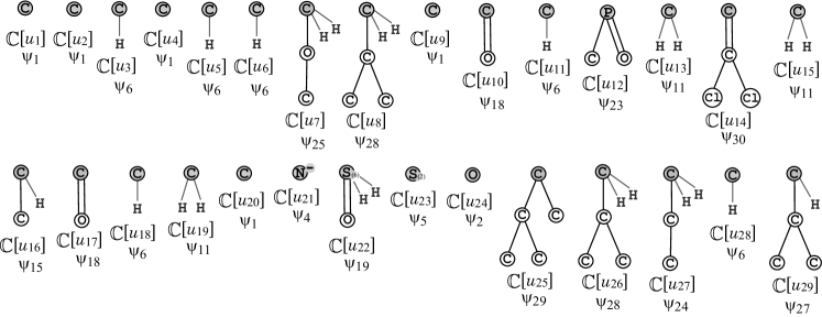
For each interior-vertex $u\in V^{\mathrm{int}}(\mathbb{C})$, let $T_{u}\in\mathcal{T}^{\mathrm{ex}}(\langle\mathbb{C}\rangle)$ denote the chemical tree rooted at $u$ (where possibly $T_{u}$ consists of vertex $u$) and define the $\rho$-fringe-tree $\mathbb{C}[u]$ to be the chemical rooted tree obtained from $T_{u}$ by putting back the hydrogens originally attached with $T_{u}$ in $\mathbb{C}$. Let $\mathcal{T}(\mathbb{C})$ denote the set of $\rho$-fringe-trees $\mathbb{C}[u],u\in V^{\mathrm{int}}(\mathbb{C})$. Figure 4 illustrates the set $\mathcal{T}(\mathbb{C})=\{\mathbb{C}[u_{i}]\mid i\in[1,29]\}$ of the 2-fringe-trees of the example $\mathbb{C}$ in Figure 3.

Figure 4: The set $\mathcal{T}^{\mathrm{ex}}(\mathbb{C})$ of 2-fringe-trees $\mathbb{C}[u_{i}],i\in[1,29]$ of $\mathbb{C}$ with $\langle\mathbb{C}\rangle$ in Figure 3, where the root of each tree is depicted with a gray circle and the hydrogens attached to non-root vertices are omitted in the figure.

Feature Function  The feature of an interior-edge $e=uv\in E^{\mathrm{int}}(\mathbb{C})$ such that $\alpha(u)={\tt a}$, $\deg_{\langle\mathbb{C}\rangle}(u)=d$, $\alpha(v)={\tt b}$, $\deg_{\langle\mathbb{C}\rangle}(v)=d^{\prime}$ and $\beta(e)=m$ is represented by a tuple $({\tt a}d,{\tt b}d^{\prime},m)$, which is called the edge-configuration of the edge $e$, where we call the tuple $({\tt a},{\tt b},m)$ the adjacency-configuration of the edge $e$.

For an integer $K$, a feature vector $f(\mathbb{C})$ of a chemical graph $\mathbb{C}$ is defined by a feature function $f$ that consists of $K$ descriptors. We call $\mathbb{R}^{K}$ the feature space.

Tanaka et al. [31] defined a feature vector $f(\mathbb{C})\in\mathbb{R}^{K}$ to be a combination of the frequency of edge-configurations of the interior-edges and the frequency of chemical rooted trees among the set of chemical rooted trees $\mathbb{C}[u]$ over all interior-vertices $u$. Zhu et al. [26] additionally included two descriptors that feature the leaf-edges and the rank of a chemical graph. In this paper, we further introduce new descriptors that features the link-edges in the monomer representation of polymers (see Appendix B for all descriptors in our feature function on polymers). Note that introduction of new descriptors requires us to modify the subsystem of simulating the computation process of a feature function $f$ in an MILP $\mathcal{M}(x,y;\mathcal{C}_{1})$. We use the same MILP formulation used by Zhu et al. [26] for $\mathcal{M}(x,y;\mathcal{C}_{1})$ by making a necessary modification (see Appendix E for the details of our MILP formulation $\mathcal{M}(g,x;\mathcal{C}_{2})$).

Topological Specification  Tanaka et al. [31] also introduced a set of rules for describing a topological specification in the following way:

1. a seed graph $G_{\mathrm{C}}$ as an abstract form of a target chemical graph $\mathbb{C}$;

2. a set $\mathcal{F}$ of chemical rooted trees as candidates for a tree $\mathbb{C}[u]$ rooted at each interior-vertex $u$ in $\mathbb{C}$; and

3. lower and upper bounds on the number of components in a target chemical graph such as chemical elements, double/triple bonds and the interior-vertices in $\mathbb{C}$.

Figure 5: (a) A seed graph $G_{\mathrm{C}}$ with $E_{\mathrm{C}}^{\mathrm{lnk}}=\{a_{1},a_{2}\}$, where the vertices in $V_{\mathrm{C}}$ are depicted with gray circles, the edges in $E_{(\geq 2)}$ are depicted with dotted lines, the edges in $E_{(\geq 1)}$ are depicted with dashed lines, the edges in $E_{(0/1)}$ are depicted with gray bold lines and the edges in $E_{(=1)}$ are depicted with black solid lines; (b) A set $\mathcal{F}=\{\psi_{1},\psi_{2},\ldots,\psi_{30}\}\subseteq\mathcal{F}(D_{\pi})$ of 30 chemical rooted trees $\psi_{i},i\in[1,30]$, where the root of each tree is depicted with a gray circle, where the hydrogens attached to non-root vertices are omitted in the figure.

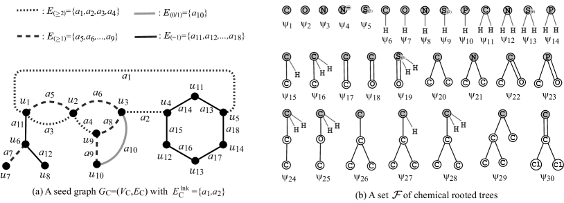
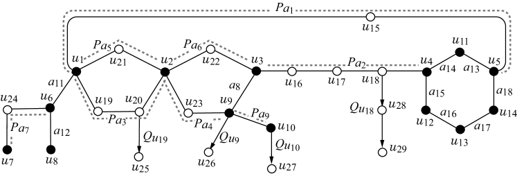
Figure 5(a) and (b) illustrate examples of a seed graph $G_{\mathrm{C}}$ and a set $\mathcal{F}$ of chemical rooted trees, respectively. Given a seed graph $G_{\mathrm{C}}$, the interior of a target chemical graph $\mathbb{C}$ is constructed from $G_{\mathrm{C}}$ by replacing some edges $a=uv$ with paths $P_{a}$ between the end-vertices $u$ and $v$ and by attaching new paths $Q_{v}$ to some vertices $v$. For example, the chemical graph $\langle\mathbb{C}\rangle$ in Figure 3 is constructed from the seed graph $G_{\mathrm{C}}$ in Figure 5(a) as follows.

1. First replace nine edges $a_{1}=u_{1}u_{5},a_{2}=u_{3}u_{4},a_{3}=u_{1}u_{2},a_{4}=u_{2}u_{9}$, $a_{5}=u_{1}u_{2},a_{6}=u_{2}u_{3},a_{7}=u_{6}u_{7},a_{8}=u_{3}u_{9}$ and $a_{9}=u_{9}u_{10}$ in $G_{\mathrm{C}}$ with new paths $P_{a_{1}}=(u_{1},u_{15},u_{5})$, $P_{a_{2}}=(u_{3},u_{16},u_{17},u_{18},u_{4})$, $P_{a_{3}}=(u_{1},u_{19},u_{20},u_{2})$, $P_{a_{4}}=(u_{2},u_{23},u_{9})$, $P_{a_{5}}=(u_{1},u_{21},u_{2})$, $P_{a_{6}}=(u_{2},u_{22},u_{3})$, $P_{a_{7}}=(u_{6},u_{24},u_{7})$, $P_{a_{8}}=(u_{3},u_{9})=a_{8}$ and $P_{a_{9}}=(u_{9},u_{10})$, respectively to obtain a subgraph $G_{1}$ of $\langle\mathbb{C}\rangle$.

2. Next attach to this graph $G_{1}$ three new paths $Q_{u_{9}}=(u_{9},u_{26})$, $Q_{u_{10}}=(u_{10},u_{27})$, $Q_{u_{18}}=(u_{18},u_{28},u_{29})$ and $Q_{u_{20}}=(u_{20},u_{25})$ to obtain the interior of $\langle\mathbb{C}\rangle$, as illustrated in Figure 6.

3. Finally attach to the interior 29 trees selected from the set $\mathcal{F}$ and assign chemical elements and bond-multiplicities in the interior to obtain a chemical graph $\mathbb{C}$ in Figure 3. In Figure 4, $\psi_{1}\in\mathcal{F}$ is selected for $\mathbb{C}[u_{i}]$, $i\in\{1,2,4,9,20\}$. Similarly $\psi_{2}$ for $\mathbb{C}[u_{24}]$, $\psi_{4}$ for $\mathbb{C}[u_{21}]$, $\psi_{5}$ for $\mathbb{C}[u_{23}]$, $\psi_{6}$ for $\mathbb{C}[u_{i}]$, $i\in\{3,5,6,11,18,28\}$, $\psi_{11}$ for $\mathbb{C}[u_{i}]$, $i\in\{13,15,19\}$, $\psi_{15}$ for $\mathbb{C}[u_{16}]$, $\psi_{18}$ for $\mathbb{C}[u_{i}]$, $i\in\{10,17\}$, $\psi_{19}$ for $\mathbb{C}[u_{22}]$, $\psi_{23}$ for $\mathbb{C}[u_{12}]$, $\psi_{24}$ for $\mathbb{C}[u_{27}]$, $\psi_{25}$ for $\mathbb{C}[u_{7}]$, $\psi_{27}$ for $\mathbb{C}[u_{29}]$, $\psi_{28}$ for $\mathbb{C}[u_{i}]$, $i\in\{8,26\}$, $\psi_{29}$ for $\mathbb{C}[u_{25}]$ and $\psi_{30}$ for $\mathbb{C}[u_{14}]$.

Figure 6: A graph obtained from the seed graph $G_{\mathrm{C}}$ in Figure 5(a), where each path $Q_{u}$ rooted at a vertex $u$ is depicted with arrows and the vertices newly introduced from $G_{\mathrm{C}}$ are depicted with white circles.

Our definition of a topological specification is analogous with the one by Zhu et al. [26] except for a necessary modification due to our polymer model with link-edges (see Appendix C for a full description of topological specification).

4 Computational Results

We implemented our method of Stages 1 to 5 for inferring chemical graphs under a given topological specification and conducted experiments to evaluate the computational efficiency. We executed the experiments on a PC with Processor: Core i7-9700 (3.0GHz; 4.7 GHz at the maximum) and Memory: 16 GB RAM DDR4.

Results on Phase 1. We have conducted experiments of linear regression for ten chemical properties on polymers among which we report the following eight properties to which the test coefficient of determination ${\rm R}^{2}$ attains at least 0.76: experimental amorphous density (AmD), dielectric constant (DeC), heat capacity liquid (HcL), heat capacity solid (HcS), mol volume (MlV), permittivity (Prm), refractive index (RfId) and glass transition(Tg). All these data sets are provided by Bicerano [36], where we did not include any polymer whose chemical formula could not be found by its name in the book. For property RfId, we remove the following polymer as an outlier from the original data set: 2-decyl-1$\underline{~{}}$4-butadiene $\mathbb{C}$ with $a(\mathbb{C})=0.4899$.

We implemented Stages 1, 2 and 3 in Phase 1 as follows.

Stage 1. We set a graph class $\mathcal{G}$ to be the set of all polymers with any graph structure, and set a branch-parameter ${\rho}$ to be 2. We represent a polymer as a monomer representation.

For each of the properties, we first select a set $\Lambda$ of chemical elements and then collect a data set $D_{\pi}$ on the polymers over the set $\Lambda$ of chemical elements. To construct the data set $D_{\pi}$, we eliminated chemical compounds such that the monomer representation $\mathbb{C}$ that does not satisfy one of the following: $\mathbb{C}$ is connected; the number of non-hydrogen neighbors of each atom $\mathbb{C}$ is at most 4; and the number of end-vertices of the linked-edges in $\mathbb{C}$ is at least two (i.e., no self-loop is a link-edge in the monomer form). Since the observed values of property Prm are measured by different frequencies, we include an extra descriptor $\mathrm{fq}$ that represents the frequency used for each polymer $\mathbb{C}_{i}\in D_{\pi}$ in our feature vector $f(\mathbb{C}_{i})$.

Table 1 shows the size and range of data sets that we prepared for each chemical property in Stage 1, where we denote the following:

1. $\Lambda$: the set of elements used in the data set $D_{\pi}$; $\Lambda$ is one of the following six sets: $\Lambda_{1}=\{{\tt H},{\tt C},{\tt O},{\tt N}\}$; $\Lambda_{2}=\{{\tt H},{\tt C},{\tt O}_{(1)},{\tt O}_{(2)},{\tt N}\}$; $\Lambda_{3}=\{{\tt H},{\tt C},{\tt O},{\tt N},{\tt Cl}\}$; $\Lambda_{4}=\{{\tt H},{\tt C},{\tt O},{\tt N},{\tt Cl},{\tt S}_{(2)}\}$; $\Lambda_{5}=\{{\tt H},{\tt C},{\tt O},{\tt N},{\tt Cl},{\tt S}_{(2)},{\tt S}_{(6)}\}$; and $\Lambda_{6}=\{{\tt H},{\tt C},{\tt O}_{(1)},{\tt O}_{(2)},{\tt N},{\tt Cl},{\tt Si}_{(4)},{\tt F}\}$, where ${\tt a}_{(i)}$ for a chemical element ${\tt a}$ and an integer $i\geq 1$ means that a chemical element ${\tt a}$ with valence $i$.

2. $|D_{\pi}|$: the size of data set $D_{\pi}$ over $\Lambda$ for the property $\pi$.

3. $\underline{n},~{}\overline{n}$: the minimum and maximum values of the number $n(\mathbb{C})$ of non-hydrogen atoms in the polymers $\mathbb{C}$ in $D_{\pi}$.

4. $\underline{a},~{}\overline{a}$: the minimum and maximum values of $a(\mathbb{C})$ for $\pi$ over the polymers $\mathbb{C}$ in $D_{\pi}$.

5. $|\Gamma|$: the number of different edge-configurations of interior-edges over the compounds in $D_{\pi}$.

6. $|\mathcal{F}|$: the number of non-isomorphic chemical rooted trees in the set of all 2-fringe-trees in the polymers in $D_{\pi}$.

7. $K$: the number of descriptors in a feature vector $f(\mathbb{C})$.

Stage 2. We used the new feature function defined in our chemical model without suppressing hydrogen (see Appendix B for the detail). We standardize the range of each descriptor and the range $\{t\in\mathbb{R}\mid\underline{a}\leq t\leq\overline{a}\}$ of property values $a(\mathbb{C}),\mathbb{C}\in D_{\pi}$.

Stage 3. For each chemical property $\pi$, we select a penalty value $\lambda_{\pi}$ in the Lasso function from 36 different values from 0 to 100 by conducting linear regression as a preliminary experiment.

We conducted an experiment in Stage 3 to evaluate the performance of the prediction function based on cross-validation. For a property $\pi$, an execution of a cross-validation consists of five trials of constructing a prediction function as follows. First partition the data set $D_{\pi}$ into five subsets $D_{\pi}^{(k)}$, $k\in[1,5]$ randomly; for each $k\in[1,5]$, the $i$-th trial constructs a prediction function $\eta(k)$ by conducting a linear regression with the penalty term $\lambda_{\pi}$ using the set $D_{\pi}\setminus D_{\pi}^{(k)}$ as a training data set. We used scikit-learn version 0.23.2 with Python 3.8.5 for executing linear regression with Lasso function. For each property, we executed ten cross-validations and we show the median of test coefficient of determination $\mathrm{R}^{2}(\eta(k),D_{\pi}^{(k)}),k\in[1,5]$ over all ten cross-validations (see Appendix A for the definition coefficient of determination $\mathrm{R}^{2}(\eta,D)$ for a prediction function $\eta$ over a data set $D$). Recall that a subset of descriptors is selected in linear regression with Lasso function and let $K^{\prime}$ denote the average number of selected descriptors over all 50 trials. The running time per trial in a cross-validation was at most one second.

Table 1: Results in Phase 1.

$\pi$	$\Lambda$	$|D_{\pi}|$	$\underline{n},~{}\overline{n}$	$\underline{a},~{}\overline{a}$	$|\Gamma|$	$|\mathcal{F}|$	$K$	$\lambda_{\pi}$	$K^{\prime}$	test $\mathrm{R}^{2}$
AmD	$\Lambda_{1}$	86	4, 45	0.838, 1.34	28	25	83	$5.0\mathrm{E}{-4}$	17.7	0.914
AmD	$\Lambda_{4}$	93	4, 45	0.838, 1.45	31	30	94	$6.0\mathrm{E}{-4}$	17.0	0.918
DeC	$\Lambda_{4}$	37	4, 22	2.13, 3.4	22	19	72	$4.0\mathrm{E}{-3}$	6.7	0.761
HcL	$\Lambda_{1}$	52	4, 25	105.7, 677.8	22	17	67	$7.0\mathrm{E}{-4}$	14.2	0.990
HcL	$\Lambda_{5}$	55	4, 32	105.7, 678.1	27	20	81	$2.0\mathrm{E}{-4}$	28.3	0.987
HcS	$\Lambda_{1}$	54	4, 45	84.5, 720.5	26	20	75	$5.0\mathrm{E}{-4}$	16.4	0.968
HcS	$\Lambda_{5}$	59	4, 45	84.5, 720.5	32	24	92	$5.0\mathrm{E}{-4}$	18.9	0.961
MlV	$\Lambda_{1}$	86	4, 45	60.7, 466.6	28	25	83	$2.0\mathrm{E}{-5}$	39.1	0.996
MlV	$\Lambda_{4}$	93	4, 45	60.7, 466.6	31	30	94	$2.0\mathrm{E}{-6}$	60.8	0.994
Prm	$\Lambda_{1}$	112	4, 45	2.23, 4.91	25	15	69	$4.0\mathrm{E}{-5}$	23.7	0.801
Prm	$\Lambda_{3}$	131	4, 45	2.23, 4.91	25	17	73	$5.0\mathrm{E}{-5}$	27.3	0.784
RfId	$\Lambda_{2}$	91	4, 29	1.4507, 1.683	26	35	96	$9.0\mathrm{E}{-4}$	22.0	0.852
RfId	$\Lambda_{6}$	124	4, 29	1.339, 1.683	32	50	124	$9.0\mathrm{E}{-4}$	27.8	0.832
Tg	$\Lambda_{1}$	204	4, 58	171, 673	32	36	101	$9.0\mathrm{E}{-5}$	40.0	0.902
Tg	$\Lambda_{5}$	232	4, 58	171, 673	36	43	118	$9.0\mathrm{E}{-5}$	45.8	0.894

Table 1 shows the results on Stages 2 and 3, where we denote the following:

1. $\lambda_{\pi}$: the penalty value in the Lasso function selected for a property $\pi$, where $a\mathrm{E}{b}$ means $a\times 10^{b}$;

2. $K^{\prime}$: the average of the number of descriptors selected in the linear regression over all 50 trials in ten cross-validations;

3. test $\mathrm{R}^{2}$: the median of test coefficient of determination $\mathrm{R}^{2}$ over all 50 trials in ten cross-validations.

From Table 1, we see that the number $K^{\prime}$ of selected descriptors is around 15 to 50 over all properties $\pi$ and that the number $K^{\prime}$ becomes slightly larger when the set $\Lambda$ of specified chemical elements is large for the same property $\pi$.

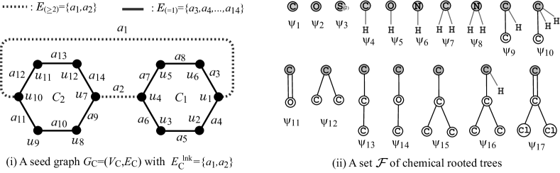
Results on Phase 2. To execute Stages 4 and 5 in Phase 2, we used a set of two instances $I_{\mathrm{a}}$ and $I_{\mathrm{b}}$. We here present their seed graphs $G_{\mathrm{C}}$ (see Appendices C and D for the details of them). The seed graph $G_{\mathrm{C}}$ of instance $I_{\mathrm{a}}$ is given by the graph in Figure 5(a). Instance $I_{\mathrm{b}}$ is introduced to represent a set of polymers that includes the four examples of polymers in Figure 7. The seed graph of instance $I_{\mathrm{b}}$ is illustrated in Figure 8(a).

Figure 7: An illustration of four polymers: (i) 1$\underline{~{}}$1-(2-methylPropane)Bis(4-phenyl)carbonate; (ii) 2$\underline{~{}}$2-pentaneBis(4-phenyl)carbonate; (iii) 1$\underline{~{}}$1-dichloroethyleneBis(4-phenyl)carbonate; (iv) thioBis(4-phenyl)carbonate, where hydrogens are omitted and connecting edges are depicted with thick lines.

Figure 8: (i) A seed graph $G_{\mathrm{C}}$ for $I_{\mathrm{b}}$; (ii) A set $\mathcal{F}$ of chemical rooted trees.

Stage 4. We executed Stage 4 for four properties $\pi\in\{$AmD, HcL, RfId, Tg$\}$. For the MILP formulation $\mathcal{M}(x,y;\mathcal{C}_{1})$ in Section A, we use the prediction function $\eta_{w,b}$ that attained the median test $\mathrm{R}^{2}$ in Table 1. To solve an MILP in Stage 4, we used CPLEX version 12.10.

For property Prm, we also need to specify the frequency $\mathrm{fq}$ under which the value $a(\mathbb{C})$ is observed, and set lower and upper bounds $\underline{\mathrm{fq}},\overline{\mathrm{fq}}\in\mathbb{R}$ on the frequency to be $\underline{\mathrm{fq}}:=60$ and $\overline{\mathrm{fq}}:=1.0\times 10^{7}$ in this experiment.

Tables 2 shows the computational results of the experiment in Stage 4 for the four properties AmD, HcL, Prm, RfId and Tg, respectively, where we denote the following:

1. $\pi$: a property $\pi\in\{$AmD, HcL, RfId, Tg$\}$;

2. inst.: instance $I_{\mathrm{a}}$ or $I_{\mathrm{b}}$;

3. $n_{\mathrm{LB}}$: a lower bound on the number of non-hydrogen atoms;

4. $\underline{y}^{*},~{}\overline{y}^{*}$: lower and upper bounds $\underline{y}^{*},\overline{y}^{*}\in\mathbb{R}$ on the value $a(\mathbb{C})$ of a polymer $\mathbb{C}$ to be inferred;

5. $\#$v (resp., $\#$c): the number of variables (resp., constraints) in the MILP in Stage 4;

6. I-time: the time (sec.) to solve the MILP in Stage 4;

7. $n$: the number $n(\mathbb{C}^{\dagger})$ of non-hydrogen atoms in the monomer representation $\mathbb{C}^{\dagger}$ inferred in Stage 4, where “none” means that no desired polymer exists for the topological specification;

8. $\mathrm{n}^{\mathrm{int}}$: the number $\mathrm{n}^{\mathrm{int}}(\mathbb{C}^{\dagger})$ of interior-vertices in the monomer representation $\mathbb{C}^{\dagger}$ inferred in Stage 4; and

9. $\eta$: the predicted property value $\eta(f(\mathbb{C}^{\dagger}))$ of the polymer $\mathbb{C}^{\dagger}$ inferred in Stage 4.

Table 2: Results of Stages 4 and 5.

$\pi$	inst.	$n_{\mathrm{LB}}$	$\underline{y}^{*},~{}\overline{y}^{*}$	$\#$v	$\#$c	I-time	$n$  $\mathrm{n}^{\mathrm{int}}$	$\eta$	D-time	$\mathbb{C}$-LB	$\#\mathbb{C}$
AmD	$I_{\mathrm{a}}$	30	0.885, 0.890	11247	12964	6.20	49 30	0.889	0.285	64	64
	$I_{\mathrm{b}}$	25	1.344, 1.350	7125	7690	2.54	28 22	1.347	0.188	2610	100
HcL	$I_{\mathrm{a}}$	30	105.7, 678.1	12171	13017	31.0	none	-	-	-	-
	$I_{\mathrm{b}}$	30	658.8, 660.2	8469	9916	1.51	32 20	660.0	0.189	576	100
Prm	$I_{\mathrm{a}}$	30	4.128 4.150	9878	12547	10.7	50 30	4.150	0.166	24	24
	$I_{\mathrm{b}}$	35	3.158 3.188	8999	12112	2.03	41 24	3.188	0.190	$1.5\mathrm{E}4$	100
RfId	$I_{\mathrm{a}}$	30	1.339, 1.683	9979	12661	92.1	none	-	-	-	-
	$I_{\mathrm{b}}$	40	1.406, 1.422	10460	15035	2.61	47 27	1.413	0.202	$7.8\mathrm{E}5$	100
Tg	$I_{\mathrm{a}}$	30	180.0, 181.6	12245	13102	17.0	50 30	181.06	0.220	36	36
	$I_{\mathrm{b}}$	45	180.6, 182.8	12953	18549	32.8	55 28	182.20	0.196	$6.3\mathrm{E}5$	100

In Table 2, $\eta(f(\mathbb{C}^{\dagger}))$ is the predicted value of property $\pi$ of a polymer $\mathbb{C}^{\dagger}$ constructed by solving an MILP in Stage 4, where we see that each $\eta(f(\mathbb{C}^{\dagger}))$ actually satisfies the specified lower and upper bounds on a target chemical value.

We set lower and upper bounds on a target chemical value for property HcL with $\Lambda_{1}$ so that $(\underline{y}^{*},\overline{y}^{*})$ is the maximal range of the observed values over the data set $D_{\pi}$; i.e., $(\underline{y}^{*},\overline{y}^{*}):=(\underline{a},\overline{a})=(105.7,678.1)$. Similarly for property RfId with $\Lambda_{6}$, we set $(\underline{y}^{*},\overline{y}^{*}):=(\underline{a},\overline{a})=(1.339,1.683)$. For an example of $I_{\mathrm{a}}$ with AmD, it holds that $\underline{y}^{*}\leq\eta(f(\mathbb{C}^{\dagger}))\leq\overline{y}^{*}$ with $\underline{y}^{*}=0.885$, $\overline{y}^{*}=0.890$ and $\eta(f(\mathbb{C}^{\dagger}))=0.889$. For instance $I_{\mathrm{a}}$ with HcL and RfId, Table 2 reveals that there is no chemical graph that satisfies the topological specification $I_{\mathrm{a}}$. These infeasible instance and instance $I_{\mathrm{b}}$ with $\pi=$Tg took around 30 to 90 seconds. For the other cases, solving an MILP for inferring a polymer with around 50 non-hydrogen atoms in the monomer form is around 2 to 15 seconds.

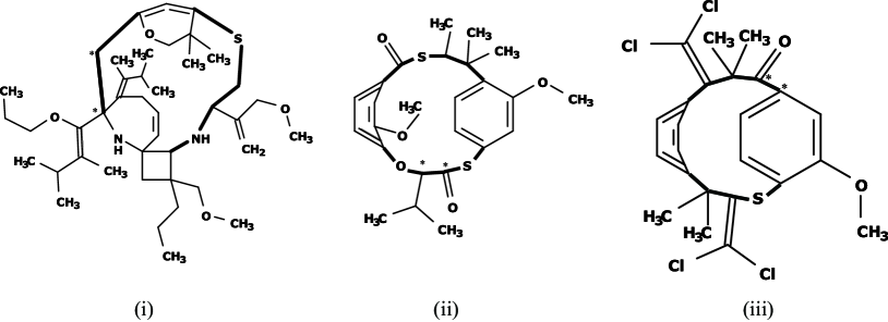
Figure 9(i) (resp., (ii)) illustrates the chemical graph $\mathbb{C}^{\dagger}$ inferred from $I_{\mathrm{a}}$ (resp., $I_{\mathrm{b}}$) with $(\underline{y}^{*},\overline{y}^{*})=(0.885,0.890)$ of AmD (resp., $(\underline{y}^{*},\overline{y}^{*})=(658.8,660.2)$ of HcL) in Table 2.

Figure 9: Illustrations of polymers, where the link-edges are depicted with thick lines and the connecting-vertices are marked with asterisks. (i) A polymer $\mathbb{C}^{\dagger}$ with $\eta(f(\mathbb{C}^{\dagger}))=0.889$ inferred from $I_{\mathrm{a}}$ with $(\underline{y}^{*},\overline{y}^{*})=(0.885,0.890)$ of AmD; (ii) A polymer $\mathbb{C}^{\dagger}$ with $\eta(f(\mathbb{C}^{\dagger}))=660.0$ inferred from $I_{\mathrm{b}}$ with $(\underline{y}^{*},\overline{y}^{*})=(658.8,660.2)$ of HcL. (iii) A polymer $\mathbb{C}^{\dagger}$ inferred from $I_{\mathrm{b}}$ with lower and upper bounds on the predicted property value $\eta_{\pi}(f(\mathbb{C}^{\dagger}))$ of property $\pi\in\{$AmD, HcL, Tg$\}$ in Table 3.

From Table 2, we observe that instances with around 30 to 55 non-hydrogen atoms in the monomer representation are solved in around 2 to 30 seconds when they are feasible.

Inferring a polymer with target values in multiple properties
Once we obtained prediction functions $\eta_{\pi}$ for several properties $\pi$, it is easy to include MILP formulations for these functions $\eta_{\pi}$ into a single MILP $\mathcal{M}(x,y;\mathcal{C}_{1})$ so as to infer a chemical graph that satisfies given target values $y^{*}$ for these properties at the same time. As an additional experiment in Stage 4, we conducted a computational experiment for inferring a polymer that has a desired predicted value each of some three properties $\pi_{1},\pi_{2}$ and $\pi_{3}$. For a combination of three properties, we selected two sets $\mathrm{P}_{1}=\{$AmD, HcL, Tg$\}$ and $\mathrm{P}_{2}=\{$HcS, MlV, RfId$\}$, where we used the prediction function $\eta_{\pi}$ for each property $\pi\in\mathrm{P}_{i}$ constructed in Stage 3. Table 3 shows the result of Stage 4 for inferring a chemical graph $\mathbb{C}^{\dagger}$ from instance $I_{\mathrm{b}}$ with a set $\Lambda(\mathrm{P}_{i})$ of chemical elements for the set $\mathrm{P}_{i}$ of properties such that $\Lambda(\mathrm{P}_{1})=\Lambda_{3}=\{{\tt H},{\tt C},{\tt O},{\tt N},{\tt Cl},{\tt S}_{(2)}\}$ and $\Lambda(\mathrm{P}_{2})=\{{\tt H},{\tt C},{\tt O}_{(2)},{\tt N},{\tt Cl}\}$, where we denote the following:

1. $\mathrm{P}_{i},i=1,2$: a combination of three properties, where $\mathrm{P}_{1}=\{$AmD, HcL, Tg$\}$ and $\mathrm{P}_{2}=\{$HcS, MlV, RfId$\}$;

2. $\pi$: one of the three properties in $\mathrm{P}_{i},i=1,2$ used in the experiment;

3. $\underline{y}^{*}_{\pi},~{}\overline{y}^{*}_{\pi}$: lower and upper bounds $\underline{y}^{*}_{\pi},\overline{y}^{*}_{\pi}\in\mathbb{R}$ on the predicted property value $\eta_{\pi}(f(\mathbb{C}^{\dagger}))$ of property $\pi\in\mathrm{P}_{i},i=1,2$ for a polymer $\mathbb{C}^{\dagger}$ to be inferred;

4. $\#$v (resp., $\#$c): the number of variables (resp., constraints) in the MILP in Stage 4;

5. I-time: the time (sec.) to solve the MILP in Stage 4;

6. $n$: the number $n(\mathbb{C}^{\dagger})$ of non-hydrogen atoms in the monomer representation $\mathbb{C}^{\dagger}$ inferred in Stage 4; and

7. $\mathrm{n}^{\mathrm{int}}$: the number $\mathrm{n}^{\mathrm{int}}(\mathbb{C}^{\dagger})$ of interior-vertices in the monomer representation $\mathbb{C}^{\dagger}$ inferred in Stage 4;

8. $\eta_{\pi}$: the predicted property value $\eta_{\pi}(f(\mathbb{C}^{\dagger}))$ of property $\pi\in\mathrm{P}_{i},i=1,2$ for the polymer $\mathbb{C}^{\dagger}$ inferred in Stage 4.

Table 3: Results of Stage 4 for instance $I_{\mathrm{b}}$ with specified target values of the three properties in $\mathrm{P}_{i},i=1,2$.

$\mathrm{P}_{i}$	$n_{\mathrm{LB}}$	$\pi$	$\underline{y}_{\pi}^{*},~{}\overline{y}_{\pi}^{*}$	$\#$v	$\#$c	I-time	$n$	$\mathrm{n}^{\mathrm{int}}$	$\eta_{\pi}$
		AmD	1.200, 1.224						1.217
$\mathrm{P}_{1}$	25	HcL	624.0, 628.0	7525	8211	3.09	31	18	625.9
		Tg	171.0, 174.0						171.55
		HcS	539, 541						540.7
$\mathrm{P}_{2}$	45	MlV	393, 395	12162	18536	210.2	45	29	394.3
		RfId	1.4507, 1.479						1.46

Fig. 9(iii) illustrates the polymer $\mathbb{C}^{\dagger}$ inferred from $I_{\mathrm{b}}$ with $(\underline{y}^{*}_{\pi_{1}},\overline{y}^{*}_{\pi_{1}})=(1.200,1.224)$, $(\underline{y}^{*}_{\pi_{2}},\overline{y}^{*}_{\pi_{2}})=(624.0,628.0)$ and $(\underline{y}^{*}_{\pi_{3}},\overline{y}^{*}_{\pi_{3}})=(171.0,174.0)$ for $\pi_{1}=$AmD, $\pi_{2}=$HcL and $\pi_{3}=$Tg, respectively.

Stage 5. We executed Stage 5 to generate a more number of target chemical graphs $\mathbb{C}^{*}$, where we call a chemical graph $\mathbb{C}^{*}$ a chemical isomer of a target chemical graph $\mathbb{C}^{\dagger}$ of a topological specification $\sigma$ if $f(\mathbb{C}^{*})=f(\mathbb{C}^{\dagger})$ and $\mathbb{C}^{*}$ also satisfies the same topological specification $\sigma$. For this, we executed the same algorithm used by Zhu et al. [26]. We computed chemical isomers $\mathbb{C}^{*}$ of each target chemical graph $\mathbb{C}^{\dagger}$ inferred in Stage 4. We execute an algorithm for generating chemical isomers of $\mathbb{C}^{\dagger}$ up to 100 when the number of all chemical isomers exceeds 100. The algorithm can evaluate a lower bound on the total number of all chemical isomers $\mathbb{C}^{\dagger}$ without generating all of them.

Tables 2 shows the computational results of the experiment in Stage 5 for properties AmD, HcL, RfId and Tg, respectively, where we denote the following:

1. D-time: the running time (sec.) to execute the dynamic programming algorithm in Stage 5 to compute a lower bound on the number of all polymers $\mathbb{C}^{*}$ of $\mathbb{C}^{\dagger}$ and generate all (or up to 100) chemical isomers $\mathbb{C}^{*}$;

2. $\mathbb{C}$-LB: a lower bound on the number of all chemical isomers $\mathbb{C}^{*}$ of $\mathbb{C}^{\dagger}$, where $a\mathrm{E}b$ means $a\times 10^{b}$; and

3. $\#\mathbb{C}$: the number of all (or up to 100) chemical isomers $\mathbb{C}^{*}$ of $\mathbb{C}^{\dagger}$ generated in Stage 5.

From Table 2, we observe that the number of isomers $\mathbb{C}^{*}$ of an output polymer $\mathbb{C}^{\dagger}$ varies on each case, where the polymer $\mathbb{C}^{\dagger}$ admits only 24 isomers $\mathbb{C}^{*}$ for instance $I_{\mathrm{a}}$ and $\pi=$Prm and over $6.3\times 10^{5}$ for instance $I_{\mathrm{b}}$ and $\pi=$Tg. The computation time for generating at most 100 isomers $\mathbb{C}^{*}$ and estimating a lower bound $\mathbb{C}$-LB is at most 0.3 second for all cases in our experiment.

5 Concluding Remarks

In this paper, we designed a method for inferring polymers based on the framework for monomers proposed by Akutsu and Nagamochi [23]. To treat a polymer as a form of monomers with no connecting-edges, we introduce a new way of representing a polymer with a monomer form by distinguishing link-edges from other edges in polymers. Since the link-edges of a polymer are characteristic to the polymer, we included new descriptors that feature the link-edges of a polymer into our feature vector. We constructed prediction functions by linear regression for eight chemical properties on polymers in Phase 1 of the framework. We inferred polymers for the first time in Phase 2 of the framework. The results of our computational experiments suggest that the method still can infer a polymer with 50 non-hydrogen atoms in the monomer form in a reasonable running time.

There are some chemical properties on polymers to which linear regression did not provide a good prediction function. It is left as a future work to use other learning methods such as decision trees and neural networks and find new effective descriptors in order to construct a prediction function with a better performance for these chemical properties on polymers.

Appendix

Appendix A Linear Regressions

This section reviews the method for linear regression used by Zhu et al. [26] in the framework of inferring chemical graphs.

For an integer $p\geq 1$ and a vector $x\in\mathbb{R}^{p}$, the $j$-th entry of $x$ is denoted by $x(j),j\in[1,p]$.

Let $D$ be a data set of chemical graphs $\mathbb{C}$ with an observed value $a(\mathbb{C})\in\mathbb{R}$, where we denote by $a_{i}=a(\mathbb{C}_{i})$ for an indexed graph $\mathbb{C}_{i}$.

Let $f$ be a feature function that maps a chemical graph $\mathbb{C}$ to a vector $f(\mathbb{C})\in\mathbb{R}^{K}$ where we denote by $x_{i}=f(\mathbb{C}_{i})$ for an indexed graph $\mathbb{C}_{i}$. For a prediction function $\eta:\mathbb{R}^{K}\to\mathbb{R}$, define an error function

$$\mathrm{Err}(\eta;D)\triangleq\sum_{\mathbb{C}_{i}\in D}(a_{i}-\eta(f(\mathbb{C}_{i})))^{2}=\sum_{\mathbb{C}_{i}\in D}(a_{i}-\eta(x_{i}))^{2},$$

and define the coefficient of determination $\mathrm{R}^{2}(\eta,D)$ to be

$${\mathrm{R}^{2}(\eta,D)\triangleq 1-\frac{\mathrm{Err}(\eta;D)}{\sum_{\mathbb{C}_{i}\in D}(a_{i}-\widetilde{a})^{2}}\mbox{ for }\widetilde{a}=\frac{1}{|D|}\sum_{\mathbb{C}\in D}a(\mathbb{C}).}$$

For a feature space $\mathbb{R}^{K}$, a hyperplane is defined to be a pair $(w,b)$ of a vector $w\in\mathbb{R}^{K}$ and a real $b\in\mathbb{R}$. Given a hyperplane $(w,b)\in\mathbb{R}^{K+1}$, a prediction function $\eta_{w,b}:\mathbb{R}^{K}\to\mathbb{R}$ is defined by setting

$$\eta_{w,b}(x)\triangleq w\cdot x+b=\sum_{j\in[1,K]}w(j)x(j)+b.$$

We observe that such a prediction function can be represented as an ANN with an input layer with $K$ nodes $u_{j},j\in[1,K]$ and an output layer with a single node $v$ such that the weight of edge arc $(u_{j},v)$ is set to be $w(j)$, the bias of node $u$ is set to be $b$ and the activation function at node $u$ is set to be a linear function. However, a learning algorithm for an ANN may not find a set of weights $w(j),j\in[1,K]$ and $b$ that minimizes the error function, since the algorithm simply iterates modification of the current weights and biases until it terminates at a local optima in the minimization.

We wish to find a hyperplane $(w,b)$ that minimizes the error function $\mathrm{Err}(\eta_{w,b};D)$. In many cases, a feature vector $f$ contains descriptors that do not play an essential role in constructing a good prediction function. When we solve the minimization problem, the entries $w(j)$ for some descriptors $j\in[1,K]$ in the resulting hyperplane $(w,b)$ become zero, which means that these descriptors were not necessarily important for finding a prediction function $\eta_{w,b}$. It is proposed that solving the minimization with an additional penalty term $\tau$ to the error function often results in a more number of entries $w(j)=0$, reducing a set of descriptors necessary for defining a prediction function $\eta_{w,b}$. For an error function with such a penalty term, a Ridge function $\frac{1}{2|D|}\mathrm{Err}(\eta_{w,b};D)+\lambda[\sum_{j\in[1,K]}w(j)^{2}+b^{2}]$ [34] and a Lasso function $\frac{1}{2|D|}\mathrm{Err}(\eta_{w,b};D)+\lambda[\sum_{j\in[1,K]}|w(j)|+|b|]$ [35] are known, where $\lambda\in\mathbb{R}$ is a given real number.

Given a prediction function $\eta_{w,b}$, we can simulate a process of computing the output $\eta_{w,b}(x)$ for an input $x\in\mathbb{R}^{K}$ as an MILP $\mathcal{M}(x,y;\mathcal{C}_{1})$ in the framework. By solving such an MILP for a specified target value $y^{*}$, we can find a vector $x^{*}\in\mathbb{R}^{K}$ such that $\eta_{w,b}(x^{*})=y^{*}$. Instead of specifying a single target value $y^{*}$, we use lower and upper bounds $\underline{y}^{*},\overline{y}^{*}\in\mathbb{R}$ on the value $a(\mathbb{C})$ of a chemical graph $\mathbb{C}$ to be inferred. We can control the range between $\underline{y}^{*}$ and $\overline{y}^{*}$ for searching a chemical graph $\mathbb{C}$ by setting $\underline{y}^{*}$ and $\overline{y}^{*}$ to be close or different values. A desired MILP is formulated as follows.

$\mathcal{M}(x,y;\mathcal{C}_{1})$: An MILP formulation for the inverse problem to prediction function

constants:

1. A hyperplane $(w,b)$ with $w\in\mathbb{R}^{K}$ and $b\in\mathbb{R}$;

2. Real values $\underline{y}^{*},\overline{y}^{*}\in\mathbb{R}$ such that $\underline{y}^{*}<\overline{y}^{*}$;

3. A set $I_{\mathbb{Z}}$ of indices $j\in[1,K]$ such that the $j$-th descriptor $\mathrm{dcp}_{j}(\mathbb{C})$ is always an integer;

4. A set $I_{+}$ of indices $j\in[1,K]$ such that the $j$-th descriptor $\mathrm{dcp}_{j}(\mathbb{C})$ is always non-negative;

5. $\ell(j),u(j)\in\mathbb{R},j\in[1,K]$: lower and upper bounds on the $j$th-descriptor;

variables:

1. Non-negative integer variable $x(j)\in\mathbb{Z}_{+},j\in I_{\mathbb{Z}}\cap I_{+}$;

2. Integer variable $x(j)\in\mathbb{Z},j\in I_{\mathbb{Z}}\setminus I_{+}$;

3. Non-negative real variable $x(j)\in\mathbb{Z}_{+},j\in I_{+}\setminus I_{\mathbb{Z}}$;

4. Real variable $x(j)\in\mathbb{Z},j\in[1,K]\setminus(I_{\mathbb{Z}}\cup I_{+})$;

constraints:

$$\ell(j)\leq x(j)\leq u(j),j\in[1,K],$$ (1)

$$\underline{y}^{*}\leq\sum_{j\in[1,K]}w(j)x(j)+b\leq\overline{y}^{*},$$ (2)

objective function:
   none.

The number of variables and constraints in the above MILP formulation is $O(K)$. It is not difficult to see that the above MILP is an NP-hard problem.

The entire MILP for Stage 4 consists of the two MILPs $\mathcal{M}(x,y;\mathcal{C}_{1})$ and $\mathcal{M}(g,x;\mathcal{C}_{2})$ with no objective function. The latter represents the computation process of our feature function $f$ and a given topological specification. See Appendix E for the details of MILP $\mathcal{M}(g,x;\mathcal{C}_{2})$.

Appendix B A Full Description of Descriptors

Our definition of feature function is analogous with the one by Zhu et al. [26] except for a necessary modification due to our polymer model with link-edges.

Associated with the two functions $\alpha$ and $\beta$ in a chemical graph $\mathbb{C}=(H,\alpha,\beta)$, we introduce functions $\mathrm{ac}:V(E)\to(\Lambda\setminus\{{\tt H}\})\times(\Lambda\setminus\{{\tt H}\})\times[1,3]$, $\mathrm{cs}:V(E)\to(\Lambda\setminus\{{\tt H}\})\times[1,6]$ and $\mathrm{ec}:V(E)\to((\Lambda\setminus\{{\tt H}\})\times[1,6])\times((\Lambda\setminus\{{\tt H}\})\times[1,6])\times[1,3]$ in the following.

To represent a feature of the exterior of $\mathbb{C}$, a chemical rooted tree in $\mathcal{T}(\mathbb{C})$ is called a fringe-configuration of $\mathbb{C}$.

We also represent leaf-edges in the exterior of $\mathbb{C}$. For a leaf-edge $uv\in E(\langle\mathbb{C}\rangle)$ with $\deg_{\langle\mathbb{C}\rangle}(u)=1$, we define the adjacency-configuration of $e$ to be an ordered tuple $(\alpha(u),\alpha(v),\beta(uv))$. Define

$$\Gamma_{\mathrm{ac}}^{\mathrm{lf}}\triangleq\{({\tt a},{\tt b},m)\mid{\tt a},{\tt b}\in\Lambda,m\in[1,\min\{\mathrm{val}({\tt a}),\mathrm{val}({\tt b})\}]\}$$

as a set of possible adjacency-configurations for leaf-edges.

To represent a feature of an interior-vertex $v\in V^{\mathrm{int}}(\mathbb{C})$ such that $\alpha(v)={\tt a}$ and $\deg_{\langle\mathbb{C}\rangle}(v)=d$ (i.e., the number of non-hydrogen atoms adjacent to $v$ is $d$) in a chemical graph $\mathbb{C}=(H,\alpha,\beta)$, we use a pair $({\tt a},d)\in(\Lambda\setminus\{{\tt H}\})\times[1,4]$, which we call the chemical symbol $\mathrm{cs}(v)$ of the vertex $v$. We treat $({\tt a},d)$ as a single symbol ${\tt a}d$, and define $\Lambda_{\mathrm{dg}}$ to be the set of all chemical symbols $\mu={\tt a}d\in(\Lambda\setminus\{{\tt H}\})\times[1,4]$.

We define a method for featuring interior-edges as follows. Let $e=uv\in E^{\mathrm{int}}(\mathbb{C})$ be an interior-edge $e=uv\in E^{\mathrm{int}}(\mathbb{C})$ such that $\alpha(u)={\tt a}$, $\alpha(v)={\tt b}$ and $\beta(e)=m$ in a chemical graph $\mathbb{C}=(H,\alpha,\beta)$. To feature this edge $e$, we use a tuple $({\tt a},{\tt b},m)\in(\Lambda\setminus\{{\tt H}\})\times(\Lambda\setminus\{{\tt H}\})\times[1,3]$, which we call the adjacency-configuration $\mathrm{ac}(e)$ of the edge $e$. We introduce a total order $<$ over the elements in $\Lambda$ to distinguish between $({\tt a},{\tt b},m)$ and $({\tt b},{\tt a},m)$ $({\tt a}\neq{\tt b})$ notationally. For a tuple $\nu=({\tt a},{\tt b},m)$, let $\overline{\nu}$ denote the tuple $({\tt b},{\tt a},m)$.

Let $e=uv\in E^{\mathrm{int}}(\mathbb{C})$ be an interior-edge $e=uv\in E^{\mathrm{int}}(\mathbb{C})$ such that $\mathrm{cs}(u)=\mu$, $\mathrm{cs}(v)=\mu^{\prime}$ and $\beta(e)=m$ in a chemical graph $\mathbb{C}=(H,\alpha,\beta)$. To feature this edge $e$, we use a tuple $(\mu,\mu^{\prime},m)\in\Lambda_{\mathrm{dg}}\times\Lambda_{\mathrm{dg}}\times[1,3]$, which we call the edge-configuration $\mathrm{ec}(e)$ of the edge $e$. We introduce a total order $<$ over the elements in $\Lambda_{\mathrm{dg}}$ to distinguish between $(\mu,\mu^{\prime},m)$ and $(\mu^{\prime},\mu,m)$ $(\mu\neq\mu^{\prime})$ notationally. For a tuple $\gamma=(\mu,\mu^{\prime},m)$, let $\overline{\gamma}$ denote the tuple $(\mu^{\prime},\mu,m)$.

Let $\pi$ be a chemical property for which we will construct a prediction function $\eta$ from a feature vector $f(\mathbb{C})$ of a chemical graph $\mathbb{C}$ to a predicted value $y\in\mathbb{R}$ for the chemical property of $\mathbb{C}$.

We first choose a set $\Lambda$ of chemical elements and then collect a data set $D_{\pi}$ of chemical compounds $C$ whose chemical elements belong to $\Lambda$, where we regard $D_{\pi}$ as a set of chemical graphs $\mathbb{C}$ that represent the chemical compounds $C$ in $D_{\pi}$. To define the interior/exterior of chemical graphs $\mathbb{C}\in D_{\pi}$, we next choose a branch-parameter ${\rho}$, where we recommend ${\rho}=2$.

Let $\Lambda^{\mathrm{int}}(D_{\pi})\subseteq\Lambda$ (resp., $\Lambda^{\mathrm{ex}}(D_{\pi})\subseteq\Lambda$) denote the set of chemical elements used in the set $V^{\mathrm{int}}(\mathbb{C})$ of interior-vertices (resp., the set $V^{\mathrm{ex}}(\mathbb{C})$ of exterior-vertices) of $\mathbb{C}$ over all chemical graphs $\mathbb{C}\in D_{\pi}$, and $\Gamma^{\mathrm{int}}(D_{\pi})$ (resp., $\Gamma^{\mathrm{lnk}}(D_{\pi})$) denote the set of edge-configurations used in the set $E^{\mathrm{int}}(\mathbb{C})$ of interior-edges (resp., the set $E^{\mathrm{lnk}}(\mathbb{C})$ of linked-edges) in $\mathbb{C}$ over all chemical graphs $\mathbb{C}\in D_{\pi}$. Let $\mathcal{F}(D_{\pi})$ denote the set of chemical rooted trees $\psi$ r-isomorphic to a chemical rooted tree in $\mathcal{T}(\mathbb{C})$ over all chemical graphs $\mathbb{C}\in D_{\pi}$, where possibly a chemical rooted tree $\psi\in\mathcal{F}(D_{\pi})$ consists of a single chemical element ${\tt a}\in\Lambda\setminus\{{\tt H}\}$.

We define an integer encoding of a finite set $A$ of elements to be a bijection $\sigma:A\to[1,|A|]$, where we denote by $[A]$ the set $[1,|A|]$ of integers. Introduce an integer coding of each of the sets $\Lambda^{\mathrm{int}}(D_{\pi})$, $\Lambda^{\mathrm{ex}}(D_{\pi})$, $\Gamma^{\mathrm{int}}(D_{\pi})$ and $\mathcal{F}(D_{\pi})$. Let $[{\tt a}]^{\mathrm{int}}$ (resp., $[{\tt a}]^{\mathrm{ex}}$) denote the coded integer of an element ${\tt a}\in\Lambda^{\mathrm{int}}(D_{\pi})$ (resp., ${\tt a}\in\Lambda^{\mathrm{ex}}(D_{\pi})$), $[\gamma]$ denote the coded integer of an element $\gamma$ in $\Gamma^{\mathrm{int}}(D_{\pi})$ and $[\psi]$ denote an element $\psi$ in $\mathcal{F}(D_{\pi})$.

We assume that a chemical graph $\mathbb{C}$ treated in this paper satisfies $\deg_{\langle\mathbb{C}\rangle}(v)\leq 4$ in the hydrogen-suppressed graph $\langle\mathbb{C}\rangle$.

In our model, we use an integer $\mathrm{mass}^{*}({\tt a})=\lfloor 10\cdot\mathrm{mass}({\tt a})\rfloor$, for each ${\tt a}\in\Lambda$.

We define the feature vector $f(\mathbb{C})$ of a polymer $\mathbb{C}=(H,\alpha,\beta)\in D_{\pi}$ to be a vector that consists of the following non-negative integer descriptors $\mathrm{dcp}_{i}(\mathbb{C})$, $i\in[1,K]$, where $K=14+|\Lambda^{\mathrm{int}}(D_{\pi})|+|\Lambda^{\mathrm{ex}}(D_{\pi})|+|\Gamma^{\mathrm{int}}(D_{\pi})|+|\Gamma^{\mathrm{lnk}}(D_{\pi})|+|\Lambda_{\mathrm{dg}}|+|\mathcal{F}(D_{\pi})|+|\Gamma_{\mathrm{ac}}^{\mathrm{lf}}|$.

1. $\mathrm{dcp}_{1}(\mathbb{C})$: the number $|V(H)|-|V_{\tt H}|$ of non-hydrogen atoms in $\mathbb{C}$.

2. $\mathrm{dcp}_{2}(\mathbb{C})$: the number $|V^{\mathrm{int}}(\mathbb{C})|$ of interior-vertices in $\mathbb{C}$.

3. $\mathrm{dcp}_{3}(\mathbb{C})$: the number $|E^{\mathrm{lnk}}(\mathbb{C})|$ of link-edges in $\mathbb{C}$. This descriptor is newly introduced in this paper to feature a structure of polymers.

4. $\mathrm{dcp}_{4}(\mathbb{C})$: the average $\overline{\mathrm{ms}}(\mathbb{C})$ of mass^∗ over all atoms in $\mathbb{C}$;
   i.e., $\overline{\mathrm{ms}}(\mathbb{C})\triangleq\frac{1}{|V(H)|}\sum_{v\in V(H)}\mathrm{mass}^{*}(\alpha(v))$.

5. $\mathrm{dcp}_{i}(\mathbb{C})$, $i=4+d,d\in[1,4]$: the number $\mathrm{dg}_{d}^{\overline{{\tt H}}}(\mathbb{C})$ of non-hydrogen vertices $v\in V(H)\setminus V_{\tt H}$ of degree $\deg_{\langle\mathbb{C}\rangle}(v)=d$ in the hydrogen-suppressed chemical graph $\langle\mathbb{C}\rangle$.

6. $\mathrm{dcp}_{i}(\mathbb{C})$, $i=8+d,d\in[1,4]$: the number $\mathrm{dg}_{d}^{\mathrm{int}}(\mathbb{C})$ of interior-vertices of interior-degree $\deg_{\mathbb{C}^{\mathrm{int}}}(v)=d$ in the interior $\mathbb{C}^{\mathrm{int}}=(V^{\mathrm{int}}(\mathbb{C}),E^{\mathrm{int}}(\mathbb{C}))$ of $\mathbb{C}$.

7. $\mathrm{dcp}_{i}(\mathbb{C})$, $i=12+m$, $m\in[2,3]$: the number $\mathrm{bd}_{m}^{\mathrm{int}}(\mathbb{C})$ of interior-edges with bond multiplicity $m$ in $\mathbb{C}$; i.e., $\mathrm{bd}_{m}^{\mathrm{int}}(\mathbb{C})\triangleq\{e\in E^{\mathrm{int}}(\mathbb{C})\mid\beta(e)=m\}$.

8. $\mathrm{dcp}_{i}(\mathbb{C})$, $i=14+[{\tt a}]^{\mathrm{int}}$, ${\tt a}\in\Lambda^{\mathrm{int}}(D_{\pi})$: the frequency $\mathrm{na}_{\tt a}^{\mathrm{int}}(\mathbb{C})=|V_{\tt a}(\mathbb{C})\cap V^{\mathrm{int}}(\mathbb{C})|$ of chemical element ${\tt a}$ in the set $V^{\mathrm{int}}(\mathbb{C})$ of interior-vertices in $\mathbb{C}$.

9. $\mathrm{dcp}_{i}(\mathbb{C})$, $i=14+|\Lambda^{\mathrm{int}}(D_{\pi})|+[{\tt a}]^{\mathrm{ex}}$, ${\tt a}\in\Lambda^{\mathrm{ex}}(D_{\pi})$: the frequency $\mathrm{na}_{\tt a}^{\mathrm{ex}}(\mathbb{C})=|V_{\tt a}(\mathbb{C})\cap V^{\mathrm{ex}}(\mathbb{C})|$ of chemical element ${\tt a}$ in the set $V^{\mathrm{ex}}(\mathbb{C})$ of exterior-vertices in $\mathbb{C}$.

10. $\mathrm{dcp}_{i}(\mathbb{C})$, $i=14+|\Lambda^{\mathrm{int}}(D_{\pi})|+|\Lambda^{\mathrm{ex}}(D_{\pi})|+[\gamma]$, $\gamma\in\Gamma^{\mathrm{int}}(D_{\pi})$: the frequency $\mathrm{ec}_{\gamma}(\mathbb{C})$ of edge-configuration $\gamma$ in the set $E^{\mathrm{int}}(\mathbb{C})$ of interior-edges in $\mathbb{C}$.

11. $\mathrm{dcp}_{i}(\mathbb{C})$, $i=14+|\Lambda^{\mathrm{int}}(D_{\pi})|+|\Lambda^{\mathrm{ex}}(D_{\pi})|+|\Gamma^{\mathrm{int}}(D_{\pi})|+[\gamma]$, $\gamma\in\Gamma^{\mathrm{lnk}}(D_{\pi})$: the frequency $\mathrm{ec}_{\gamma}(\mathbb{C})$ of edge-configuration $\gamma$ in the set $E^{\mathrm{lnk}}(\mathbb{C})$ of link-edges in $\mathbb{C}$. This descriptor is newly introduced in this paper to feature link-edges of polymers.

12. $\mathrm{dcp}_{i}(\mathbb{C})$, $i=14+|\Lambda^{\mathrm{int}}(D_{\pi})|+|\Lambda^{\mathrm{ex}}(D_{\pi})|+|\Gamma^{\mathrm{int}}(D_{\pi})|+[\mu]$, $\mu\in\Lambda_{\mathrm{dg}}^{\mathrm{int}}$: the frequency of chemical symbols $\mu=\alpha(u)\deg_{\langle\mathbb{C}\rangle}(u)$ of connecting-vertices $u$ in $\mathbb{C}$.

13. $\mathrm{dcp}_{i}(\mathbb{C})$, $i=14+|\Lambda^{\mathrm{int}}(D_{\pi})|+|\Lambda^{\mathrm{ex}}(D_{\pi})|+|\Gamma^{\mathrm{int}}(D_{\pi})|+|\Gamma^{\mathrm{lnk}}(D_{\pi})|+|\Lambda_{\mathrm{dg}}|+[\psi]$, $\psi\in\mathcal{F}(D_{\pi})$: the frequency $\mathrm{fc}_{\psi}(\mathbb{C})$ of fringe-configuration $\psi$ in the set of ${\rho}$-fringe-trees in $\mathbb{C}$.

14. $\mathrm{dcp}_{i}(\mathbb{C})$, $i=14+|\Lambda^{\mathrm{int}}(D_{\pi})|+|\Lambda^{\mathrm{ex}}(D_{\pi})|+|\Gamma^{\mathrm{int}}(D_{\pi})|+|\Gamma^{\mathrm{lnk}}(D_{\pi})|+|\Lambda_{\mathrm{dg}}|+|\mathcal{F}(D_{\pi})|+[\nu]$, $\nu\in\Gamma_{\mathrm{ac}}^{\mathrm{lf}}$: the frequency $\mathrm{ac}_{\nu}^{\mathrm{lf}}(\mathbb{C})$ of adjacency-configuration $\nu$ in the set of leaf-edges in $\langle\mathbb{C}\rangle$.

Appendix C Specifying Target Chemical Graphs

Our definition of topological specification is analogous with the one by Zhu et al. [26] except for a necessary modification due to our polymer model with link-edges.

Seed Graph

A seed graph for a polymer is defined to be a graph $G_{\mathrm{C}}=(V_{\mathrm{C}},E_{\mathrm{C}})$ with a specified edge subset $E_{\mathrm{C}}^{\mathrm{lnk}}$ such that the edge set $E_{\mathrm{C}}$ consists of four sets $E_{(\geq 2)}$, $E_{(\geq 1)}$, $E_{(0/1)}$ and $E_{(=1)}$, where each of them can be empty, and $E_{\mathrm{C}}^{\mathrm{lnk}}$ is a circular set in $G_{\mathrm{C}}$ such that $\emptyset\neq E_{\mathrm{C}}^{\mathrm{lnk}}\subseteq E_{(\geq 2)}\cup E_{(\geq 1)}\cup E_{(=1)}$. Figure 5(a) illustrates an example of a seed graph, where $V_{\mathrm{C}}=\{u_{1},u_{2},\ldots,u_{14}\}$, $E_{(\geq 2)}=\{a_{1},a_{2},a_{3},a_{4}\}$, $E_{(\geq 1)}=\{a_{5},a_{6},\ldots,a_{9}\}$, $E_{(0/1)}=\{a_{10}\}$, $E_{(=1)}=\{a_{11},a_{12},\ldots,a_{18}\}$ and $E_{\mathrm{C}}^{\mathrm{lnk}}=\{a_{1},a_{2}\}$.

A subdivision $S$ of $G_{\mathrm{C}}$ is a graph constructed from a seed graph $G_{\mathrm{C}}$ according to the following rules:

1. Each edge $e=uv\in E_{(\geq 2)}$ is replaced with a $u,v$-path $P_{e}$ of length at least 2;

2. Each edge $e=uv\in E_{(\geq 1)}$ is replaced with a $u,v$-path $P_{e}$ of length at least 1 (equivalently $e$ is directly used or replaced with a $u,v$-path $P_{e}$ of length at least 2);

3. Each edge $e\in E_{(0/1)}$ is either used or discarded; and

4. Each edge $e\in E_{(=1)}$ is always used directly.

The set of link-edges in the monomer representation $\mathbb{C}$ of an inferred polymer consists of edges in $E_{\mathrm{C}}^{\mathrm{lnk}}\cap(E_{(=1)}\cup E_{(\geq 1)})$ or edges in paths $P_{e}$ for all edges $e=uv\in E_{\mathrm{C}}^{\mathrm{lnk}}\cap(E_{(\geq 1)}\cup E_{(\geq 2)})$ in a subdivision $S$ of $G_{\mathrm{C}}$.

A target chemical graph $\mathbb{C}=(H,\alpha,\beta)$ will contain $S$ as a subgraph of the interior $H^{\mathrm{int}}$ of $\mathbb{C}$.

Interior-specification

A graph $H^{*}$ that serves as the interior $H^{\mathrm{int}}$ of a target chemical graph $\mathbb{C}$ will be constructed as follows. First construct a subdivision $S$ of a seed graph $G_{\mathrm{C}}$ by replacing each edge $e=uu^{\prime}\in E_{(\geq 2)}\cup E_{(\geq 1)}$ with a pure $u,u^{\prime}$-path $P_{e}$. Next construct a supergraph $H^{*}$ of $S$ by attaching a leaf path $Q_{v}$ at each vertex $v\in V_{\mathrm{C}}$ or at an internal vertex $v\in V(P_{e})\setminus\{u,u^{\prime}\}$ of each pure $u,u^{\prime}$-path $P_{e}$ for some edge $e=uu^{\prime}\in E_{(\geq 2)}\cup E_{(\geq 1)}$, where possibly $Q_{v}=(v),E(Q_{v})=\emptyset$ (i.e., we do not attach any new edges to $v$). We introduce the following rules for specifying the size of $H^{*}$, the length $|E(P_{e})|$ of a pure path $P_{e}$, the length $|E(Q_{v})|$ of a leaf path $Q_{v}$, the number of leaf paths $Q_{v}$ and a bond-multiplicity of each interior-edge, where we call the set of prescribed constants an interior-specification $\sigma_{\mathrm{int}}$:

1. Lower and upper bounds $\mathrm{n}^{\mathrm{int}}_{\mathrm{LB}},\mathrm{n}^{\mathrm{int}}_{\mathrm{UB}}\in\mathbb{Z}_{+}$ on the number of interior-vertices of a target chemical graph $\mathbb{C}$.

2. Lower and upper bounds $\mathrm{n}^{\mathrm{lnk}}_{\mathrm{LB}},\mathrm{n}^{\mathrm{lnk}}_{\mathrm{UB}}\in\mathbb{Z}_{+}$ on the number of link-edges of a target chemical graph $\mathbb{C}$.

3. For each edge $e=uu^{\prime}\in E_{(\geq 2)}\cup E_{(\geq 1)}$,

   a lower bound $\ell_{\mathrm{LB}}(e)$ and an upper bound $\ell_{\mathrm{UB}}(e)$ on the length $|E(P_{e})|$ of a pure $u,u^{\prime}$-path $P_{e}$. (For a notational convenience, set $\ell_{\mathrm{LB}}(e):=0$, $\ell_{\mathrm{UB}}(e):=1$, $e\in E_{(0/1)}$ and $\ell_{\mathrm{LB}}(e):=1$, $\ell_{\mathrm{UB}}(e):=1$, $e\in E_{(=1)}$.)

   a lower bound $\mathrm{bl}_{\mathrm{LB}}(e)$ and an upper bound $\mathrm{bl}_{\mathrm{UB}}(e)$ on the number of leaf paths $Q_{v}$ attached at internal vertices $v$ of a pure $u,u^{\prime}$-path $P_{e}$.

   a lower bound $\mathrm{ch}_{\mathrm{LB}}(e)$ and an upper bound $\mathrm{ch}_{\mathrm{UB}}(e)$ on the maximum length $|E(Q_{v})|$ of a leaf path $Q_{v}$ attached at an internal vertex $v\in V(P_{e})\setminus\{u,u^{\prime}\}$ of a pure $u,u^{\prime}$-path $P_{e}$.

4. For each vertex $v\in V_{\mathrm{C}}$,

   a lower bound $\mathrm{ch}_{\mathrm{LB}}(v)$ and an upper bound $\mathrm{ch}_{\mathrm{UB}}(v)$ on the number of leaf paths $Q_{v}$ attached to $v$, where $0\leq\mathrm{ch}_{\mathrm{LB}}(v)\leq\mathrm{ch}_{\mathrm{UB}}(v)\leq 1$.

   a lower bound $\mathrm{ch}_{\mathrm{LB}}(v)$ and an upper bound $\mathrm{ch}_{\mathrm{UB}}(v)$ on the length $|E(Q_{v})|$ of a leaf path $Q_{v}$ attached to $v$.

5. For each edge $e=uu^{\prime}\in E_{\mathrm{C}}$, a lower bound $\mathrm{bd}_{m,\mathrm{LB}}(e)$ and an upper bound $\mathrm{bd}_{m,\mathrm{UB}}(e)$ on the number of edges with bond-multiplicity $m\in[2,3]$ in $u,u^{\prime}$-path $P_{e}$, where we regard $P_{e}$, $e\in E_{(0/1)}\cup E_{(=1)}$ as single edge $e$.

We call a graph $H^{*}$ that satisfies an interior-specification $\sigma_{\mathrm{int}}$ a $\sigma_{\mathrm{int}}$-extension of $G_{\mathrm{C}}$, where the bond-multiplicity of each edge has been determined.

Table 4 shows an example of an interior-specification $\sigma_{\mathrm{int}}$ to the seed graph $G_{\mathrm{C}}$ in Figure 5.

Table 4: Example 1 of an interior-specification $\sigma_{\mathrm{int}}$.

$\mathrm{n}^{\mathrm{int}}_{\mathrm{LB}}=20$

$\mathrm{n}^{\mathrm{int}}_{\mathrm{UB}}=30$

$\mathrm{n}^{\mathrm{lnk}}_{\mathrm{LB}}=2$

$\mathrm{n}^{\mathrm{lnk}}_{\mathrm{UB}}=24$

	$a_{1}$	$a_{2}$	$a_{3}$	$a_{4}$	$a_{5}$	$a_{6}$	$a_{7}$	$a_{8}$	$a_{9}$
$\ell_{\mathrm{LB}}(a_{i})$	2	4	3	2	2	1	1	1	1
$\ell_{\mathrm{UB}}(a_{i})$	3	6	6	5	3	3	6	2	6
$\mathrm{bl}_{\mathrm{LB}}(a_{i})$	0	1	1	0	0	0	0	0	0
$\mathrm{bl}_{\mathrm{UB}}(a_{i})$	1	4	4	3	2	1	1	1	1
$\mathrm{ch}_{\mathrm{LB}}(a_{i})$	0	2	1	0	0	0	0	0	0
$\mathrm{ch}_{\mathrm{UB}}(a_{i})$	3	6	6	3	3	3	3	0	0

	$u_{1}$	$u_{2}$	$u_{3}$	$u_{4}$	$u_{5}$	$u_{6}$	$u_{7}$	$u_{8}$	$u_{9}$	$u_{10}$	$u_{11}$	$u_{12}$	$u_{13}$	$u_{14}$
$\mathrm{bl}_{\mathrm{LB}}(u_{i})$	0	0	0	0	0	0	0	0	1	0	0	0	0	0
$\mathrm{bl}_{\mathrm{UB}}(u_{i})$	1	1	1	1	1	1	1	1	1	1	1	1	1	1
$\mathrm{ch}_{\mathrm{LB}}(u_{i})$	0	0	0	0	0	0	0	0	1	0	0	0	0	0
$\mathrm{ch}_{\mathrm{UB}}(u_{i})$	4	4	4	4	4	4	4	4	6	4	4	4	4	4

	$a_{1}$	$a_{2}$	$a_{3}$	$a_{4}$	$a_{5}$	$a_{6}$	$a_{7}$	$a_{8}$	$a_{9}$	$a_{10}$	$a_{11}$	$a_{12}$	$a_{13}$	$a_{14}$	$a_{15}$	$a_{16}$	$a_{17}$	$a_{18}$
$\mathrm{bd}_{2,\mathrm{LB}}(a_{i})$	0	0	0	0	0	0	0	0	0	0	0	0	0	1	0	0	0	0
$\mathrm{bd}_{2,\mathrm{UB}}(a_{i})$	1	2	1	1	1	1	1	1	1	1	1	1	1	1	1	1	1	1
$\mathrm{bd}_{3,\mathrm{LB}}(a_{i})$	0	0	0	0	0	0	0	0	0	0	0	0	0	0	0	0	0	0
$\mathrm{bd}_{3,\mathrm{UB}}(a_{i})$	1	1	1	1	1	1	1	1	1	1	1	1	1	1	1	1	1	1

Figure 6 illustrates an example of an $\sigma_{\mathrm{int}}$-extension $H^{*}$ of seed graph $G_{\mathrm{C}}$ in Figure 5(a) under the interior-specification $\sigma_{\mathrm{int}}$ in Table 4.

Chemical-specification

Let $H^{*}$ be a graph that serves as the interior $H^{\mathrm{int}}$ of a target chemical graph $\mathbb{C}$, where the bond-multiplicity of each edge in $H^{*}$ has be determined. Finally we introduce a set of rules for constructing a target chemical graph $\mathbb{C}$ from $H^{*}$ by choosing a chemical element ${\tt a}\in\Lambda$ and assigning a ${\rho}$-fringe-tree $\psi$ to each interior-vertex $v\in V^{\mathrm{int}}$. We introduce the following rules for specifying the size of $\mathbb{C}$, a set of chemical rooted trees that are allowed to use as ${\rho}$-fringe-trees and lower and upper bounds on the frequency of a chemical element, a chemical symbol, an edge-configuration, and a fringe-configuration where we call the set of prescribed constants a chemical specification $\sigma_{\mathrm{ce}}$:

1. Lower and upper bounds $n_{\mathrm{LB}},n^{*}\in\mathbb{Z}_{+}$ on the number of vertices, where $\mathrm{n}^{\mathrm{int}}_{\mathrm{LB}}\leq n_{\mathrm{LB}}\leq n^{*}$.

2. A subset $\mathcal{F}^{*}\subseteq\mathcal{F}(D_{\pi})$ of chemical rooted trees $\psi$ with $\mathrm{ht}(\langle\psi\rangle)\leq{\rho}$, where we require that every ${\rho}$-fringe-tree $\mathbb{C}[v]$ rooted at an interior-vertex $v$ in $\mathbb{C}$ belongs to $\mathcal{F}^{*}$. Let $\Lambda^{\mathrm{ex}}$ denote the set of chemical elements assigned to non-root vertices over all chemical rooted trees in $\mathcal{F}^{*}$.

3. A subset $\Lambda^{\mathrm{int}}\subseteq\Lambda^{\mathrm{int}}(D_{\pi})$, where we require that every chemical element $\alpha(v)$ assigned to an interior-vertex $v$ in $\mathbb{C}$ belongs to $\Lambda^{\mathrm{int}}$. Let $\Lambda:=\Lambda^{\mathrm{int}}\cup\Lambda^{\mathrm{ex}}$ and $\mathrm{na}_{\tt a}(\mathbb{C})$ (resp., $\mathrm{na}_{\tt a}^{\mathrm{int}}(\mathbb{C})$ and $\mathrm{na}_{\tt a}^{\mathrm{ex}}(\mathbb{C})$) denote the number of vertices (resp., interior-vertices and exterior-vertices) $v$ such that $\alpha(v)={\tt a}$ in $\mathbb{C}$.

4. A set $\Lambda_{\mathrm{dg}}^{\mathrm{int}}\subseteq\Lambda\times[1,4]$ of chemical symbols.

5. Subsets $\Gamma^{\mathrm{lnk}}\subseteq\Gamma^{\mathrm{int}}$ of $\Gamma^{\mathrm{int}}(D_{\pi})$ of edge-configurations $(\mu,\mu^{\prime},m)$ with $\mu\leq\mu^{\prime}$, where we require that the edge-configuration $\mathrm{ec}(e)$ of an interior-edge (resp., a link-edge) $e$ in $\mathbb{C}$ belongs to $\Gamma^{\mathrm{int}}$ (resp., $\Gamma^{\mathrm{lnk}}$). We do not distinguish $(\mu,\mu^{\prime},m)$ and $(\mu^{\prime},\mu,m)$.

6. Define $\Gamma_{\mathrm{ac}}^{\mathrm{int}}$ (resp., $\Gamma_{\mathrm{ac}}^{\mathrm{lnk}}$) to be the set of adjacency-configurations such that $\Gamma_{\mathrm{ac}}^{\mathrm{t}}:=\{({\tt a},{\tt b},m)\mid({\tt a}d,{\tt b}d^{\prime},m)\in\Gamma^{\mathrm{t}}\},\mathrm{t}\in\{\mathrm{int},\mathrm{lnk}\}$. Let $\mathrm{ac}_{\nu}^{\mathrm{int}}(\mathbb{C}),\nu\in\Gamma_{\mathrm{ac}}^{\mathrm{int}}$ (resp., $\mathrm{ac}_{\nu}^{\mathrm{lnk}}(\mathbb{C}),\nu\in\Gamma_{\mathrm{ac}}^{\mathrm{lnk}}$) denote the number of interior-edges (resp., link-edges) $e$ such that $\mathrm{ac}(e)=\nu$ in $\mathbb{C}$.

7. Subsets $\Lambda^{*}(v)\subseteq\{{\tt a}\in\Lambda^{\mathrm{int}}\mid\mathrm{val}({\tt a})\geq 2\}$, $v\in V_{\mathrm{C}}$, we require that every chemical element $\alpha(v)$ assigned to a vertex $v\in V_{\mathrm{C}}$ in the seed graph belongs to $\Lambda^{*}(v)$.

8. Lower and upper bound functions $\mathrm{na}_{\mathrm{LB}},\mathrm{na}_{\mathrm{UB}}:\Lambda\to[0,n^{*}]$ and $\mathrm{na}_{\mathrm{LB}}^{\mathrm{int}},\mathrm{na}_{\mathrm{UB}}^{\mathrm{int}}:\Lambda^{\mathrm{int}}\to[0,n^{*}]$ on the number of interior-vertices $v$ such that $\alpha(v)={\tt a}$ in $\mathbb{C}$.

9. Lower and upper bound functions $\mathrm{ns}_{\mathrm{LB}}^{\mathrm{int}},\mathrm{ns}_{\mathrm{UB}}^{\mathrm{int}}:\Lambda_{\mathrm{dg}}^{\mathrm{int}}\to[0,n^{*}]$ on the number of interior-vertices $v$ such that $\mathrm{cs}(v)=\mu$ in $\mathbb{C}$.

10. Lower and upper bound functions $\mathrm{ns}_{\mathrm{LB}}^{\mathrm{cnt}},\mathrm{ns}_{\mathrm{UB}}^{\mathrm{cnt}}:\Lambda_{\mathrm{dg}}^{\mathrm{int}}\to[0,2]$ on the number of connecting-vertices $v$ such that $\mathrm{cs}(v)=\mu$ in $\mathbb{C}$.

11. Lower and upper bound functions $\mathrm{ac}_{\mathrm{LB}}^{\mathrm{int}},\mathrm{ac}_{\mathrm{UB}}^{\mathrm{int}}:\Gamma_{\mathrm{ac}}^{\mathrm{int}}\to\mathbb{Z}_{+}$ ($\mathrm{ac}_{\mathrm{LB}}^{\mathrm{lnk}},\mathrm{ac}_{\mathrm{UB}}^{\mathrm{lnk}}:\Gamma_{\mathrm{ac}}^{\mathrm{lnk}}\to\mathbb{Z}_{+}$) on the number of interior-edges (resp., link-edges) $e$ such that $\mathrm{ac}(e)=\nu$ in $\mathbb{C}$.

12. Lower and upper bound functions $\mathrm{ec}_{\mathrm{LB}}^{\mathrm{int}},\mathrm{ec}_{\mathrm{UB}}^{\mathrm{int}}:\Gamma^{\mathrm{int}}\to\mathbb{Z}_{+}$ (resp., $\mathrm{ec}_{\mathrm{LB}}^{\mathrm{lnk}},\mathrm{ec}_{\mathrm{UB}}^{\mathrm{lnk}}:\Gamma^{\mathrm{lnk}}\to\mathbb{Z}_{+}$) on the number of interior-edges (resp., link-edges) $e$ such that $\mathrm{ec}(e)=\gamma$ in $\mathbb{C}$.

13. Lower and upper bound functions $\mathrm{fc}_{\mathrm{LB}},\mathrm{fc}_{\mathrm{UB}}:\mathcal{F}^{*}\to[0,n^{*}]$ on the number of interior-vertices $v$ such that $\mathbb{C}[v]^{\mathrm{fr}}$ is r-isomorphic to $\psi\in\mathcal{F}^{*}$ in $\mathbb{C}$.

14. Lower and upper bound functions $\mathrm{ac}^{\mathrm{lf}}_{\mathrm{LB}},\mathrm{ac}^{\mathrm{lf}}_{\mathrm{UB}}:\Gamma_{\mathrm{ac}}^{\mathrm{lf}}\to[0,n^{*}]$ on the number of leaf-edges $uv$ in $\mathrm{ac}_{\mathrm{C}}$ with adjacency-configuration $\nu$.

We call a chemical graph $\mathbb{C}$ that satisfies a chemical specification $\sigma_{\mathrm{ce}}$ a $(\sigma_{\mathrm{int}},\sigma_{\mathrm{ce}})$-extension of $G_{\mathrm{C}}$, and denote by $\mathcal{G}(G_{\mathrm{C}},\sigma_{\mathrm{int}},\sigma_{\mathrm{ce}})$ the set of all $(\sigma_{\mathrm{int}},\sigma_{\mathrm{ce}})$-extensions of $G_{\mathrm{C}}$.

Table 5 shows an example of a chemical-specification $\sigma_{\mathrm{ce}}$ to the seed graph $G_{\mathrm{C}}$ in Figure 5.

Table 5: Example 2 of a chemical-specification $\sigma_{\mathrm{ce}}$.

$n_{\mathrm{LB}}=30$, $n^{*}=50$.

branch-parameter: ${\rho}=2$

Each of sets $\mathcal{F}(v),v\in V_{\mathrm{C}}$ and $\mathcal{F}_{E}$ is set to be

the set $\mathcal{F}$ of chemical rooted trees $\psi$ with $\mathrm{ht}(\langle\psi\rangle)\leq{\rho}=2$ in Figure 5(b).

$\Lambda=\{{\tt H},{\tt C},{\tt N},{\tt O},{\tt S}_{(2)},{\tt S}_{(6)},{\tt P}={\tt P}_{(6)},{\tt Cl}\}$

$\Lambda_{\mathrm{dg}}^{\mathrm{int}}=\{{\tt C}2,{\tt C}3,{\tt C}4,{\tt N}2,{\tt N}3,{\tt O}2,{\tt S}_{(2)}2,{\tt S}_{(6)}3,{\tt P}4\}$

$\Gamma_{\mathrm{ac}}^{\mathrm{int}}$

$\nu_{1}\!=\!({\tt C},{\tt C},1),\nu_{2}\!=\!({\tt C},{\tt C},2),\nu_{3}\!=\!({\tt C},{\tt N},1),\nu_{4}\!=\!({\tt C},{\tt O},1),\nu_{5}\!=\!({\tt C},{\tt S}_{(2)},1),\nu_{6}\!=\!({\tt C},{\tt S}_{(6)},1),\nu_{7}\!=\!({\tt C},{\tt P},1)$

$\Gamma^{\mathrm{int}}$	$\gamma_{1}\!=\!({\tt C}2,{\tt C}2,1),\gamma_{2}\!=\!({\tt C}2,{\tt C}2,2),\gamma_{3}\!=\!({\tt C}2,{\tt C}3,1),\gamma_{4}\!=\!({\tt C}2,{\tt C}3,2),\gamma_{5}\!=\!({\tt C}2,{\tt C}4,1),\gamma_{6}\!=\!({\tt C}3,{\tt C}3,1),$
	$\gamma_{7}\!=\!({\tt C}3,{\tt C}3,2),\gamma_{8}\!=\!({\tt C}3,{\tt C}4,1),\gamma_{9}\!=\!({\tt C}2,{\tt N}3,1),\gamma_{10}\!=\!({\tt C}3,{\tt N}2,1),\gamma_{11}\!=\!({\tt C}4,{\tt N}2,1),\gamma_{12}\!=\!({\tt C}2,{\tt O}2,1),$
	$\gamma_{13}\!=\!({\tt C}3,{\tt O}2,1),\gamma_{14}\!=\!({\tt C}2,{\tt S}_{(2)}2,1),\gamma_{15}\!=\!({\tt C}3,{\tt S}_{(2)}2,1),\gamma_{16}\!=\!({\tt C}4,{\tt S}_{(2)}2,1),\gamma_{17}\!=\!({\tt C}3,{\tt S}_{(6)}3,1),$
	$\gamma_{18}\!=\!({\tt C}4,{\tt S}_{(6)}3,1),\gamma_{19}\!=\!({\tt C}2,{\tt P}4,1),\gamma_{20}\!=\!({\tt C}3,{\tt P}4,1)$

$\Gamma_{\mathrm{ac}}^{\mathrm{lnk}}$

$\nu^{\prime}_{1}\!=\!({\tt C},{\tt C},1),\nu^{\prime}_{2}\!=\!({\tt C},{\tt C},2),\nu^{\prime}_{3}\!=\!({\tt C},{\tt N},1),\nu^{\prime}_{4}\!=\!({\tt C},{\tt S}_{(2)},1)$

$\Gamma^{\mathrm{lnk}}$	$\gamma^{\prime}_{1}\!=\!({\tt C}2,{\tt C}2,1),\gamma^{\prime}_{2}\!=\!({\tt C}2,{\tt C}3,1),\gamma^{\prime}_{3}\!=\!({\tt C}2,{\tt C}4,1),\gamma^{\prime}_{4}\!=\!({\tt C}3,{\tt C}3,1),\gamma^{\prime}_{5}\!=\!({\tt C}3,{\tt C}3,2),\gamma^{\prime}_{6}\!=\!({\tt C}2,{\tt N}3,1),$
	$\gamma^{\prime}_{7}\!=\!({\tt C}3,{\tt N}2,1),\gamma^{\prime}_{8}\!=\!({\tt C}2,{\tt S}_{(2)}2,1),\gamma^{\prime}_{9}\!=\!({\tt C}3,{\tt S}_{(2)}2,1),\gamma^{\prime}_{10}\!=\!({\tt C}4,{\tt S}_{(2)}2,1)$

$\Lambda^{*}(u_{i})=\{{\tt C}\},i\in\{1,2,3,4,5,6,9\}$, $\Lambda^{*}(u_{8})=\{{{\tt O}}\}$, $\Lambda^{*}(u_{12})=\{{\tt C,P}\}$,

$\Lambda^{*}(u_{i})=\{{\tt C},{\tt O},{\tt N}\}$, $i\in[1,14]\setminus\{1,2,3,4,5,6,8,9,12\}$

	${\tt H}$	${\tt C}$	${\tt N}$	${\tt O}$	${\tt S}_{(2)}$	${\tt S}_{(6)}$	${\tt P}$	${\tt Cl}$
$\mathrm{na}_{\mathrm{LB}}({\tt a})$	40	25	1	1	0	0	0	0
$\mathrm{na}_{\mathrm{UB}}({\tt a})$	80	50	8	8	4	4	4	4

	${\tt C}$	${\tt N}$	${\tt O}$	${\tt S}_{(2)}$	${\tt S}_{(6)}$	${\tt P}$
$\mathrm{na}_{\mathrm{LB}}^{\mathrm{int}}({\tt a})$	10	1	0	0	0	0
$\mathrm{na}_{\mathrm{UB}}^{\mathrm{int}}({\tt a})$	25	4	5	2	2	2

	${\tt C}2$	${\tt C}3$	${\tt C}4$	${\tt N}2$	${\tt N}3$	${\tt O}2$	${\tt S}_{(2)}2$	${\tt S}_{(6)}3$	${\tt P}4$
$\mathrm{ns}_{\mathrm{LB}}^{\mathrm{int}}(\mu)$	3	5	0	0	0	0	0	0	0
$\mathrm{ns}_{\mathrm{UB}}^{\mathrm{int}}(\mu)$	12	15	5	5	3	5	1	1	1

	${\tt C}2$	${\tt C}3$	${\tt C}4$	${\tt N}2$	${\tt N}3$	${\tt O}2$	${\tt S}_{(2)}2$	${\tt S}_{(6)}3$	${\tt P}4$
$\mathrm{ns}_{\mathrm{LB}}^{\mathrm{cnt}}(\mu)$	0	0	0	0	0	0	0	0	0
$\mathrm{ns}_{\mathrm{UB}}^{\mathrm{cnt}}(\mu)$	2	2	2	2	2	2	1	1	0

	$\nu_{1}$	$\nu_{2}$	$\nu_{3}$	$\nu_{4}$	$\nu_{5}$	$\nu_{6}$	$\nu_{7}$
$\mathrm{ac}_{\mathrm{LB}}^{\mathrm{int}}(\nu)$	0	0	0	0	0	0	0
$\mathrm{ac}_{\mathrm{UB}}^{\mathrm{int}}(\nu)$	30	10	10	10	2	3	3

	$\gamma_{1}$	$\gamma_{2}$	$\gamma_{3}$	$\gamma_{4}$	$\gamma_{5}$	$\gamma_{i},i\in[6,13]$	$\gamma_{i},i\in[14,20]$
$\mathrm{ec}_{\mathrm{LB}}^{\mathrm{int}}(\gamma)$	0	0	0	0	0	0	0
$\mathrm{ec}_{\mathrm{UB}}^{\mathrm{int}}(\gamma)$	4	15	5	5	10	5	2

	$\nu^{\prime}_{1}$	$\nu^{\prime}_{2}$	$\nu^{\prime}_{3}$	$\nu^{\prime}_{4}$
$\mathrm{ac}_{\mathrm{LB}}^{\mathrm{lnk}}(\nu^{\prime})$	0	0	0	0
$\mathrm{ac}_{\mathrm{UB}}^{\mathrm{lnk}}(\nu^{\prime})$	10	5	5	5

	$\gamma^{\prime}_{i},i\in[1,10]$
$\mathrm{ec}_{\mathrm{LB}}^{\mathrm{lnk}}(\gamma^{\prime})$	0
$\mathrm{ec}_{\mathrm{UB}}^{\mathrm{lnk}}(\gamma^{\prime})$	4

	$\psi\in\{\psi_{i}\mid i=1,6,11\}$	$\psi\in\mathcal{F}^{*}\setminus\{\psi_{i}\mid i=1,6,11\}$
$\mathrm{fc}_{\mathrm{LB}}(\psi)$	1	0
$\mathrm{fc}_{\mathrm{UB}}(\psi)$	10	3

	$\nu\in\{({\tt C},{\tt C},1),({\tt C},{\tt C},2)\}$	$\nu\in\Gamma_{\mathrm{ac}}^{\mathrm{lf}}\setminus\{({\tt C},{\tt C},1),({\tt C},{\tt C},2)\}$
$\mathrm{ac}^{\mathrm{lf}}_{\mathrm{LB}}(\nu)$	0	0
$\mathrm{ac}^{\mathrm{lf}}_{\mathrm{UB}}(\nu)$	10	8

Figure 3 illustrates an example of a $(\sigma_{\mathrm{int}},\sigma_{\mathrm{ce}})$-extension of $G_{\mathrm{C}}$ obtained from the $\sigma_{\mathrm{int}}$-extension $H^{*}$ in Figure 6 under the chemical-specification $\sigma_{\mathrm{ce}}$ in Table 5.

Appendix D Test Instances for Stages 4 and 5

We prepared the following instances $I_{\mathrm{a}}$ and $I_{\mathrm{b}}$ for conducting experiments of Stages 4 and 5 in Phase 2.

In Stages 4 and 5, we use four properties $\pi\in\{$AmD, HcL, RfId, Tg$\}$ and define a set $\Lambda(\pi)$ of chemical elements as follows: $\Lambda($AmD$)=\Lambda_{4}=\{{\tt H},{\tt C},{\tt N},{\tt O},{\tt Cl},{\tt S}_{(2)}\}$, $\Lambda($HcL$)=\Lambda($Tg$)=\Lambda_{5}=\{{\tt H},{\tt C},{\tt O},{\tt N},{\tt Cl},{\tt S}_{(2)},{\tt S}_{(6)}\}$, $\Lambda($RfId$)=\Lambda_{6}=\{{\tt H},{\tt C},{\tt O}_{(1)},{\tt O}_{(2)},{\tt N},{\tt Cl},{\tt Si}_{(4)},{\tt F}\}$ and $\Lambda($Prm$)=\Lambda_{3}=\{{\tt H},{\tt C},{\tt O},{\tt N},{\tt Cl}\}$.

• $I_{\mathrm{a}}=(G_{\mathrm{C}},\sigma_{\mathrm{int}},\sigma_{\mathrm{ce}})$: The instance used in Appendix C to explain the target specification. For each property $\pi\in\{$AmD, HcL, RfId, Tg, Prm$\}$, we replace $\Lambda=\{{\tt H},{\tt C},{\tt N},{\tt O},{\tt S}_{(2)},{\tt S}_{(6)},{\tt P}_{(5)},{\tt Cl}\}$ in Table 5 with $\Lambda(\pi)\cap\{{\tt S}_{(2)},{\tt S}_{(6)},{\tt P}_{(5)},{\tt Cl}\}$ and remove from the $\sigma_{\mathrm{ce}}$ all chemical symbols, edge-configurations and fringe-configurations that cannot be constructed from the replaced element set (i.e., those containing a chemical element in $\{{\tt S}_{(2)},{\tt S}_{(6)},{\tt P}_{(5)},{\tt Cl}\}\setminus\Lambda(\pi)$).

• $I_{\mathrm{b}}=(G_{\mathrm{C}},\sigma_{\mathrm{int}},\sigma_{\mathrm{ce}})$: An instance that represents a set of polymers that includes the four examples of polymers in Fig. 7. We set a seed graph $G_{\mathrm{C}}=(V_{\mathrm{C}},E_{\mathrm{C}}=E_{(=1)})$ to be the graph with two cycles $C_{1}$ and $C_{2}$ in Fig. 8(a), where we set $E_{(\geq 2)}=E_{\mathrm{C}}^{\mathrm{lnk}}=\{a_{1},a_{2}\}$ and $E_{(=1)}=\{a_{3},a_{12},\ldots,a_{14}\}$.
  Set $\Lambda:=\Lambda(\pi)$ for each property $\pi\in\{$AmD, HcL, RfId, Tg$\}$, and set $\Lambda_{\mathrm{dg}}^{\mathrm{int}}$ to be the set of all possible chemical symbols in $\Lambda\times[1,4]$.
  Set $\Gamma^{\mathrm{int}}$ (resp., $\Gamma^{\mathrm{lnk}}$) to be the set of edge-configurations of the interior-edges (resp., the link-edges) used in the four examples of polymers in Fig. 7. Set $\Gamma^{\mathrm{int}}_{\mathrm{ac}}$ (resp., $\Gamma^{\mathrm{lnk}}_{\mathrm{ac}}$) to be the set of the adjacency-configurations of the edge-configurations in $\Gamma^{\mathrm{int}}$ (resp., $\Gamma^{\mathrm{lnk}}$).
  We specify $n_{\mathrm{LB}}$ for each property $\pi$ and set $\mathrm{n}^{\mathrm{int}}_{\mathrm{LB}}:=14$, $\mathrm{n}^{\mathrm{int}}_{\mathrm{UB}}:=n^{*}:=n_{\mathrm{LB}}+10$, $\mathrm{n}^{\mathrm{lnk}}_{\mathrm{LB}}:=2$, $\mathrm{n}^{\mathrm{lnk}}_{\mathrm{UB}}:=2+\max\{n_{\mathrm{LB}}-15,0\}$.
  For each link-edge $a_{i}\in E_{(\geq 2)}=E_{\mathrm{C}}^{\mathrm{lnk}}=\{a_{1},a_{2}\}$, set $\ell_{\mathrm{LB}}(a_{i}):=2+\max\{\lfloor(n_{\mathrm{LB}}-15)/4\rfloor,0\}$, $\ell_{\mathrm{UB}}(a_{i}):=\ell_{\mathrm{LB}}(a_{i})+5$, $\mathrm{bl}_{\mathrm{LB}}(a_{i}):=0,\mathrm{bl}_{\mathrm{UB}}(a_{i}):=3$, $\mathrm{ch}_{\mathrm{LB}}(a_{i}):=0,\mathrm{ch}_{\mathrm{UB}}(a_{i}):=5$, $\mathrm{bd}_{2,\mathrm{LB}}(a_{i}):=0$ and $\mathrm{bd}_{2,\mathrm{UB}}(a_{i}):=\lfloor\ell_{\mathrm{LB}}(a_{i})/3\rfloor$.
  To form two benzene rings from the two cycles $C_{1}$ and $C_{2}$, set $\Lambda^{*}(u):=\{{\tt C}\}$, $\mathrm{bl}_{\mathrm{LB}}(u):=\mathrm{bl}_{\mathrm{UB}}(u):=\mathrm{ch}_{\mathrm{LB}}(u):=\mathrm{ch}_{\mathrm{UB}}(u):=0$, $u\in V_{\mathrm{C}}$, $\mathrm{bd}_{2,\mathrm{LB}}(a_{i}):=\mathrm{bd}_{2,\mathrm{UB}}(a_{i}):=0,i\in\{3,5,7,9,11,13\}$, $\mathrm{bd}_{2,\mathrm{LB}}(a_{i}):=\mathrm{bd}_{2,\mathrm{UB}}(a_{i}):=1,i\in\{4,6,8,10,12,14\}$.
  Not to include any triple-bond, set $\mathrm{bd}_{3,\mathrm{LB}}(a):=\mathrm{bd}_{3,\mathrm{UB}}(a):=0,a\in E_{\mathrm{C}}$.
  Set lower bounds $\mathrm{na}_{\mathrm{LB}}$, $\mathrm{na}^{\mathrm{int}}_{\mathrm{LB}}$, $\mathrm{ns}^{\mathrm{int}}_{\mathrm{LB}}$, $\mathrm{ns}^{\mathrm{cnt}}_{\mathrm{LB}}$, $\mathrm{ac}^{\mathrm{int}}_{\mathrm{LB}}$, $\mathrm{ac}_{\mathrm{LB}}^{\mathrm{lnk}}$, $\mathrm{ec}_{\mathrm{LB}}^{\mathrm{int}}$, $\mathrm{ec}_{\mathrm{LB}}^{\mathrm{lnk}}$ and $\mathrm{ac}^{\mathrm{lf}}_{\mathrm{LB}}$ to be 0.
  Set upper bounds $\mathrm{na}_{\mathrm{UB}}({\tt a}):=n^{*},\mathrm{na}\in\{{\tt H},{\tt C}\}$, $\mathrm{na}_{\mathrm{UB}}({\tt a}):=5+\max\{n_{\mathrm{LB}}-15,0\},{\tt a}\in\{{\tt O},{\tt N}\}$, $\mathrm{na}_{\mathrm{UB}}({\tt a}):=2+\max\{\lfloor(n_{\mathrm{LB}}-15)/4\rfloor,0\},{\tt a}\in\Lambda\setminus\{{\tt H},{\tt C},{\tt O},{\tt N}\}$, $\mathrm{ns}^{\mathrm{cnt}}_{\mathrm{UB}}(\mu):=2,\mu\in\Lambda_{\mathrm{dg}}^{\mathrm{int}}$, and $\mathrm{na}^{\mathrm{int}}_{\mathrm{UB}}$, $\mathrm{ns}^{\mathrm{int}}_{\mathrm{UB}}$, $\mathrm{ac}^{\mathrm{int}}_{\mathrm{UB}}$, $\mathrm{ac}_{\mathrm{LB}}^{\mathrm{lnk}}$, $\mathrm{ec}_{\mathrm{UB}}^{\mathrm{int}}$, $\mathrm{ec}_{\mathrm{UB}}^{\mathrm{lnk}}$ and $\mathrm{ac}^{\mathrm{lf}}_{\mathrm{UB}}$ to be $n^{*}$.
  Set $\mathcal{F}$ to be the set of the 17 chemical rooted trees $\psi_{i},i\in[1,17]$ in Fig. 8(b). Set $\mathcal{F}_{E}:=\mathcal{F}(v):=\mathcal{F}$, $v\in V_{\mathrm{C}}$ and $\mathrm{fc}_{\mathrm{LB}}(\psi):=0,\psi\in\mathcal{F}$, $\mathrm{fc}_{\mathrm{UB}}(\psi_{i}):=12+\max\{n_{\mathrm{LB}}-15,0\},i\in[1,4]$, $\mathrm{fc}_{\mathrm{UB}}(\psi_{i}):=8+\max\{\lfloor(n_{\mathrm{LB}}-15)/2\rfloor,0\},i\in[5,12]$ and $\mathrm{fc}_{\mathrm{UB}}(\psi_{i}):=5+\max\{\lfloor(n_{\mathrm{LB}}-15)/4\rfloor,0\},i\in[13,17],\psi_{i}\in\mathcal{F}$.

Appendix E All Constraints in an MILP Formulation for Chemical Graphs

Our definition of an MILP formulation MILP $\mathcal{M}(g,x;\mathcal{C}_{2})$ is analogous with the one by Zhu et al. [26] except for a necessary modification due to our polymer model with link-edges.

We define a standard encoding of a finite set $A$ of elements to be a bijection $\sigma:A\to[1,|A|]$, where we denote by $[A]$ the set $[1,|A|]$ of integers and by $[{\tt e}]$ the encoded element $\sigma({\tt e})$. Let $\epsilon$ denote null, a fictitious chemical element that does not belong to any set of chemical elements, chemical symbols, adjacency-configurations and edge-configurations in the following formulation. Given a finite set $A$, let $A_{\epsilon}$ denote the set $A\cup\{\epsilon\}$ and define a standard encoding of $A_{\epsilon}$ to be a bijection $\sigma:A\to[0,|A|]$ such that $\sigma(\epsilon)=0$, where we denote by $[A_{\epsilon}]$ the set $[0,|A|]$ of integers and by $[{\tt e}]$ the encoded element $\sigma({\tt e})$, where $[\epsilon]=0$.

Let $\sigma=(G_{\mathrm{C}},\sigma_{\mathrm{int}},\sigma_{\mathrm{ce}})$ be a target specification, ${\rho}$ denote the branch-parameter in the specification $\sigma$ and $\mathbb{C}$ denote a chemical graph in $\mathcal{G}(G_{\mathrm{C}},\sigma_{\mathrm{int}},\sigma_{\mathrm{ce}})$.

E.1 Selecting a Cyclical-base

Recall that

$$\begin{array}[]{ll}E_{(=1)}=\{e\in E_{\mathrm{C}}\mid\ell_{\mathrm{LB}}(e)=\ell_{\mathrm{UB}}(e)=1\};&E_{(0/1)}=\{e\in E_{\mathrm{C}}\mid\ell_{\mathrm{LB}}(e)=0,\ell_{\mathrm{UB}}(e)=1\};\\ E_{(\geq 1)}=\{e\in E_{\mathrm{C}}\mid\ell_{\mathrm{LB}}(e)=1,\ell_{\mathrm{UB}}(e)\geq 2\};&E_{(\geq 2)}=\{e\in E_{\mathrm{C}}\mid\ell_{\mathrm{LB}}(e)\geq 2\};\end{array}$$

A subset $E_{\mathrm{C}}^{\mathrm{lnk}}\subseteq E_{(=1)}\cup E_{(\geq 1)}\cup E_{(\geq 2)}$ is given for introducing link-edges in the monomer representation $\mathbb{C}$ of an inferred polymer.

1. Every edge $a_{i}\in E_{(=1)}$ is included in $\langle\mathbb{C}\rangle$;

2. Each edge $a_{i}\in E_{(0/1)}$ is included in $\langle\mathbb{C}\rangle$ if necessary;

3. For each edge $a_{i}\in E_{(\geq 2)}$, edge $a_{i}$ is not included in $\langle\mathbb{C}\rangle$ and instead a path

   $$P_{i}=({v^{\mathrm{C}}}_{\mathrm{tail}(i)},{v^{\mathrm{T}}}_{j-1},{v^{\mathrm{T}}}_{j},\ldots,{v^{\mathrm{T}}}_{j+t},{v^{\mathrm{C}}}_{\mathrm{head}(i)})$$

   of length at least 2 from vertex ${v^{\mathrm{C}}}_{\mathrm{tail}(i)}$ to vertex ${v^{\mathrm{C}}}_{\mathrm{head}(i)}$ visiting some vertices in $V_{\mathrm{T}}$ is constructed in $\langle\mathbb{C}\rangle$; and

4. For each edge $a_{i}\in E_{(\geq 1)}$, either edge $a_{i}$ is directly used in $\langle\mathbb{C}\rangle$ or the above path $P_{i}$ of length at least 2 is constructed in $\langle\mathbb{C}\rangle$.

Let ${t_{\mathrm{C}}}\triangleq|V_{\mathrm{C}}|$ and denote $V_{\mathrm{C}}$ by $\{{v^{\mathrm{C}}}_{i}\mid i\in[1,{t_{\mathrm{C}}}]\}$. Regard the seed graph $G_{\mathrm{C}}$ as a digraph such that each edge $a_{i}$ with end-vertices ${v^{\mathrm{C}}}_{j}$ and ${v^{\mathrm{C}}}_{j^{\prime}}$ is directed from ${v^{\mathrm{C}}}_{j}$ to ${v^{\mathrm{C}}}_{j^{\prime}}$ when $j<j^{\prime}$. For each directed edge $a_{i}\in E_{\mathrm{C}}$, let $\mathrm{head}(i)$ and $\mathrm{tail}(i)$ denote the head and tail of ${e^{\mathrm{C}}}(i)$; i.e., $a_{i}=({v^{\mathrm{C}}}_{\mathrm{tail}(i)},{v^{\mathrm{C}}}_{\mathrm{head}(i)})$.

Define

$${k_{\mathrm{C}}}\triangleq|E_{(\geq 2)}\cup E_{(\geq 1)}|,~{}~{}\widetilde{{k_{\mathrm{C}}}}\triangleq|E_{(\geq 2)}|,$$

and denote $E_{\mathrm{C}}=\{a_{i}\mid i\in[1,m_{\mathrm{C}}]\}$,

$$E_{(\geq 2)}=\{a_{k}\mid k\in[1,\widetilde{{k_{\mathrm{C}}}}]\} E_{(\geq 1)}=\{a_{k}\mid k\in[\widetilde{{k_{\mathrm{C}}}}+1,{k_{\mathrm{C}}}]\}$$, ,

$$E_{(0/1)}=\{a_{i}\mid i\in[{k_{\mathrm{C}}}+1,{k_{\mathrm{C}}}+|E_{(0/1)}|]\} E_{(=1)}=\{a_{i}\mid i\in[{k_{\mathrm{C}}}+|E_{(0/1)}|+1,m_{\mathrm{C}}]\}$$ and .

Let $I_{(=1)}$ denote the set of indices $i$ of edges $a_{i}\in E_{(=1)}$. Similarly for $I_{(0/1)}$, $I_{(\geq 1)}$ and $I_{(\geq 2)}$. Let $I_{\mathrm{lnk}}$ denote the set of indices $i$ of edges $a_{i}\in E_{\mathrm{C}}^{\mathrm{lnk}}$.

To control the construction of such a path $P_{i}$ for each edge $a_{k}\in E_{(\geq 2)}\cup E_{(\geq 1)}$, we regard the index $k\in[1,{k_{\mathrm{C}}}]$ of each edge $a_{k}\in E_{(\geq 2)}\cup E_{(\geq 1)}$ as the “color” of the edge. To introduce necessary linear constraints that can construct such a path $P_{k}$ properly in our MILP, we assign the color $k$ to the vertices ${v^{\mathrm{T}}}_{j-1},{v^{\mathrm{T}}}_{j},\ldots,$ ${v^{\mathrm{T}}}_{j+t}$ in $V_{\mathrm{T}}$ when the above path $P_{k}$ is used in $\langle\mathbb{C}\rangle$.

For each index $s\in[1,{t_{\mathrm{C}}}]$, let ${I_{\mathrm{C}}}(s)$ denote the set of edges $e\in E_{\mathrm{C}}$ incident to vertex ${v^{\mathrm{C}}}_{s}$, and $E_{(=1)}^{+}(s)$ (resp., $E_{(=1)}^{-}(s)$) denote the set of edges $a_{i}\in E_{(=1)}$ such that the tail (resp., head) of $a_{i}$ is vertex ${v^{\mathrm{C}}}_{s}$. Similarly for $E_{(0/1)}^{+}(s)$, $E_{(0/1)}^{-}(s)$, $E_{(\geq 1)}^{+}(s)$, $E_{(\geq 1)}^{-}(s)$, $E_{(\geq 2)}^{+}(s)$ and $E_{(\geq 2)}^{-}(s)$. Let ${I_{\mathrm{C}}}(s)$ denote the set of indices $i$ of edges $a_{i}\in{I_{\mathrm{C}}}(s)$. Similarly for $I_{(=1)}^{+}(s)$, $I_{(=1)}^{-}(s)$, $I_{(0/1)}^{+}(s)$, $I_{(0/1)}^{-}(s)$, $I_{(\geq 1)}^{+}(s)$, $I_{(\geq 1)}^{-}(s)$, $I_{(\geq 2)}^{+}(s)$ and $I_{(\geq 2)}^{-}(s)$. Note that $[1,{k_{\mathrm{C}}}]=I_{(\geq 2)}\cup I_{(\geq 1)}$ and $[\widetilde{{k_{\mathrm{C}}}}+1,m_{\mathrm{C}}]=I_{(\geq 1)}\cup I_{(0/1)}\cup I_{(=1)}$.

constants:

1. $n^{*}\in\mathbb{Z}$: an upper bound on the number $n(\mathbb{C})$ of non-hydrogen atoms in $\mathbb{C}$;

2. ${t_{\mathrm{C}}}=|V_{\mathrm{C}}|$, $\widetilde{{k_{\mathrm{C}}}}=|E_{(\geq 2)}|$, ${k_{\mathrm{C}}}=|E_{(\geq 2)}\cup E_{(\geq 1)}|$, ${t_{\mathrm{T}}}=\mathrm{n}^{\mathrm{int}}_{\mathrm{UB}}-|V_{\mathrm{C}}|$, $m_{\mathrm{C}}=|E_{\mathrm{C}}|$. Note that $a_{i}\in E_{\mathrm{C}}\setminus(E_{(\geq 2)}\cup E_{(\geq 1)})$ holds $i\in[{k_{\mathrm{C}}}+1,m_{\mathrm{C}}]$;

3. $\ell_{\mathrm{LB}}(k),\ell_{\mathrm{UB}}(k)\in[1,{t_{\mathrm{T}}}]$, $k\in[1,{k_{\mathrm{C}}}]$: lower and upper bounds on the length of path $P_{k}$;

4. $n_{\mathrm{lnk}}^{(=1)}=|I_{\mathrm{lnk}}\cap E_{(=1)}|=|I_{\mathrm{lnk}}\cap\{[{k_{\mathrm{C}}}+|E_{(0/1)}|+1,m_{\mathrm{C}}\}|$: the number of link-edges created from $E_{(=1)}$;

5. $\mathrm{n}^{\mathrm{lnk}}_{\mathrm{LB}},\mathrm{n}^{\mathrm{lnk}}_{\mathrm{UB}}\in[0,n^{*}]$: lower and upper bounds on the number of link-edges of a target polymer $\mathbb{C}$;

variables:

1. ${e^{\mathrm{C}}}(i)\in[0,1]$, $i\in[1,m_{\mathrm{C}}]$: ${e^{\mathrm{C}}}(i)$ represents edge $a_{i}\in E_{\mathrm{C}}$, $i\in[1,m_{\mathrm{C}}]$ (${e^{\mathrm{C}}}(i)=1$, $i\in I_{(=1)}$; ${e^{\mathrm{C}}}(i)=0$, $i\in I_{(\geq 2)}$) (${e^{\mathrm{C}}}(i)=1$ $\Leftrightarrow$ edge $a_{i}$ is used in $\langle\mathbb{C}\rangle$);

2. ${v^{\mathrm{T}}}(i)\in[0,1]$, $i\in[1,{t_{\mathrm{T}}}]$: ${v^{\mathrm{T}}}(i)=1$ $\Leftrightarrow$ vertex ${v^{\mathrm{T}}}_{i}$ is used in $\langle\mathbb{C}\rangle$;

3. ${e^{\mathrm{T}}}(i)\in[0,1]$, $i\in[1,{t_{\mathrm{T}}}+1]$: ${e^{\mathrm{T}}}(i)$ represents edge ${e^{\mathrm{T}}}_{i}=({v^{\mathrm{T}}}_{i-1},{v^{\mathrm{T}}}_{i})\in E_{\mathrm{T}}$, where ${e^{\mathrm{T}}}_{1}$ and ${e^{\mathrm{T}}}_{{t_{\mathrm{T}}}+1}$ are fictitious edges (${e^{\mathrm{T}}}(i)=1$ $\Leftrightarrow$ edge ${e^{\mathrm{T}}}_{i}$ is used in $\langle\mathbb{C}\rangle$);

4. ${\chi^{\mathrm{T}}}(i)\in[0,{k_{\mathrm{C}}}]$, $i\in[1,{t_{\mathrm{T}}}]$: ${\chi^{\mathrm{T}}}(i)$ represents the color assigned to vertex ${v^{\mathrm{T}}}_{i}$ (${\chi^{\mathrm{T}}}(i)=k>0$ $\Leftrightarrow$ vertex ${v^{\mathrm{T}}}_{i}$ is assigned color $k$; ${\chi^{\mathrm{T}}}(i)=0$ means that vertex ${v^{\mathrm{T}}}_{i}$ is not used in $\langle\mathbb{C}\rangle$);

5. $\mathrm{clr}^{\mathrm{T}}(k)\in[\ell_{\mathrm{LB}}(k)-1,\ell_{\mathrm{UB}}(k)-1]$, $k\in[1,{k_{\mathrm{C}}}]$, $\mathrm{clr}^{\mathrm{T}}(0)\in[0,{t_{\mathrm{T}}}]$: the number of vertices ${v^{\mathrm{T}}}_{i}\in V_{\mathrm{T}}$ with color $c$;

6. $\delta_{\chi}^{\mathrm{T}}(k)\in[0,1]$, $k\in[0,{k_{\mathrm{C}}}]$: $\delta_{\chi}^{\mathrm{T}}(k)=1$ $\Leftrightarrow$ ${\chi^{\mathrm{T}}}(i)=k$ for some $i\in[1,{t_{\mathrm{T}}}]$;

7. ${\chi^{\mathrm{T}}}(i,k)\in[0,1]$, $i\in[1,{t_{\mathrm{T}}}]$, $k\in[0,{k_{\mathrm{C}}}]$ (${\chi^{\mathrm{T}}}(i,k)=1$ $\Leftrightarrow$ ${\chi^{\mathrm{T}}}(i)=k$);

8. ${\widetilde{\deg}_{\mathrm{C}}}^{+}(i)\in[0,4]$, $i\in[1,{t_{\mathrm{C}}}]$: the out-degree of vertex ${v^{\mathrm{C}}}_{i}$ with the used edges ${e^{\mathrm{C}}}$ in $E_{\mathrm{C}}$;

9. ${\widetilde{\deg}_{\mathrm{C}}}^{-}(i)\in[0,4]$, $i\in[1,{t_{\mathrm{C}}}]$: the in-degree of vertex ${v^{\mathrm{C}}}_{i}$ with the used edges ${e^{\mathrm{C}}}$ in $E_{\mathrm{C}}$;

10. $n_{\mathrm{lnk}}\in[\mathrm{n}^{\mathrm{lnk}}_{\mathrm{LB}},\mathrm{n}^{\mathrm{lnk}}_{\mathrm{UB}}]$: the number of link-edges in $\mathbb{C}$;

constraints:

$${e^{\mathrm{C}}}(i)=1,~{}~{}~{}i\in I_{(=1)},$$ (3)

$${e^{\mathrm{C}}}(i)=0,~{}~{}\mathrm{clr}^{\mathrm{T}}(i)\geq 1,~{}~{}~{}i\in I_{(\geq 2)},$$ (4)

$${e^{\mathrm{C}}}(i)+\mathrm{clr}^{\mathrm{T}}(i)\geq 1,~{}~{}~{}~{}~{}\mathrm{clr}^{\mathrm{T}}(i)\leq{t_{\mathrm{T}}}\cdot(1-{e^{\mathrm{C}}}(i)),~{}~{}~{}i\in I_{(\geq 1)},$$ (5)

$$\sum_{c\in I_{(\geq 1)}^{-}(i)\cup I_{(0/1)}^{-}(i)\cup I_{(=1)}^{-}(i)}\!\!\!\!\!\!{e^{\mathrm{C}}}(c)={\widetilde{\deg}_{\mathrm{C}}}^{-}(i),~{}~{}\sum_{c\in I_{(\geq 1)}^{+}(i)\cup I_{(0/1)}^{+}(i)\cup I_{(=1)}^{+}(i)}\!\!\!\!\!\!{e^{\mathrm{C}}}(c)={\widetilde{\deg}_{\mathrm{C}}}^{+}(i), i\in[1,{t_{\mathrm{C}}}],$$ (6)

$${\chi^{\mathrm{T}}}(i,0)=1-{v^{\mathrm{T}}}(i),~{}~{}~{}\sum_{k\in[0,{k_{\mathrm{C}}}]}{\chi^{\mathrm{T}}}(i,k)=1,~{}~{}~{}\sum_{k\in[0,{k_{\mathrm{C}}}]}k\cdot{\chi^{\mathrm{T}}}(i,k)={\chi^{\mathrm{T}}}(i), i\in[1,{t_{\mathrm{T}}}],$$ (7)

$$\sum_{i\in[1,{t_{\mathrm{T}}}]}{\chi^{\mathrm{T}}}(i,k)=\mathrm{clr}^{\mathrm{T}}(k),~{}~{}{t_{\mathrm{T}}}\cdot\delta_{\chi}^{\mathrm{T}}(k)\geq\sum_{i\in[1,{t_{\mathrm{T}}}]}{\chi^{\mathrm{T}}}(i,k)\geq\delta_{\chi}^{\mathrm{T}}(k), k\in[0,{k_{\mathrm{C}}}],$$ (8)

$${v^{\mathrm{T}}}(i-1)\geq{v^{\mathrm{T}}}(i),$$

$${k_{\mathrm{C}}}\cdot({v^{\mathrm{T}}}(i-1)-{e^{\mathrm{T}}}(i))\geq{\chi^{\mathrm{T}}}(i-1)-{\chi^{\mathrm{T}}}(i)\geq{v^{\mathrm{T}}}(i-1)-{e^{\mathrm{T}}}(i), i\in[2,{t_{\mathrm{T}}}],$$ (9)

$$\sum_{k\in I_{\mathrm{lnk}}\cap[1,{k_{\mathrm{C}}}]}(\mathrm{clr}^{\mathrm{T}}(k)+1)+n_{\mathrm{lnk}}^{(=1)}=n_{\mathrm{lnk}}.$$ (10)

E.2 Constraints for Including Leaf Paths

Let $\widetilde{{t_{\mathrm{C}}}}$ denote the number of vertices $u\in V_{\mathrm{C}}$ such that $\mathrm{bl}_{\mathrm{UB}}(u)=1$ and assume that $V_{\mathrm{C}}=\{u_{1},u_{2},\ldots,u_{p}\}$ so that

$$\mathrm{bl}_{\mathrm{UB}}(u_{i})=1 i\in[1,\widetilde{{t_{\mathrm{C}}}}] \mathrm{bl}_{\mathrm{UB}}(u_{i})=0 i\in[\widetilde{{t_{\mathrm{C}}}}+1,{t_{\mathrm{C}}}]$$, and , .

Define the set of colors for the vertex set $\{u_{i}\mid i\in[1,\widetilde{{t_{\mathrm{C}}}}]\}\cup V_{\mathrm{T}}$ to be $[1,{c_{\mathrm{F}}}]$ with

$${c_{\mathrm{F}}}\triangleq\widetilde{{t_{\mathrm{C}}}}+{t_{\mathrm{T}}}=|\{u_{i}\mid i\in[1,\widetilde{{t_{\mathrm{C}}}}]\}\cup V_{\mathrm{T}}|.$$

Let each vertex ${v^{\mathrm{C}}}_{i}$, $i\in[1,\widetilde{{t_{\mathrm{C}}}}]$ (resp., ${v^{\mathrm{T}}}_{i}\in V_{\mathrm{T}}$) correspond to a color $i\in[1,{c_{\mathrm{F}}}]$ (resp., $i+\widetilde{{t_{\mathrm{C}}}}\in[1,{c_{\mathrm{F}}}]$). When a path $P=(u,{v^{\mathrm{F}}}_{j},{v^{\mathrm{F}}}_{j+1},\ldots,{v^{\mathrm{F}}}_{j+t})$ from a vertex $u\in V_{\mathrm{C}}\cup V_{\mathrm{T}}$ is used in $\langle\mathbb{C}\rangle$, we assign the color $i\in[1,{c_{\mathrm{F}}}]$ of the vertex $u$ to the vertices ${v^{\mathrm{F}}}_{j},{v^{\mathrm{F}}}_{j+1},\ldots,{v^{\mathrm{F}}}_{j+t}\in V_{\mathrm{F}}$.

constants:

1. ${c_{\mathrm{F}}}$: the maximum number of different colors assigned to the vertices in $V_{\mathrm{F}}$;

2. $\mathrm{n}^{\mathrm{int}}_{\mathrm{LB}},\mathrm{n}^{\mathrm{int}}_{\mathrm{UB}}\in[2,n^{*}]$: lower and upper bounds on the number of interior-vertices in $\mathbb{C}$;

3. $\mathrm{bl}_{\mathrm{LB}}(i)\in[0,1]$, $i\in[1,\widetilde{{t_{\mathrm{C}}}}]$: a lower bound on the number of leaf ${\rho}$-branches in the leaf path rooted at a vertex ${v^{\mathrm{C}}}_{i}$;

4. $\mathrm{bl}_{\mathrm{LB}}(k),\mathrm{bl}_{\mathrm{UB}}(k)\in[0,\ell_{\mathrm{UB}}(k)-1]$, $k\in[1,{k_{\mathrm{C}}}]=I_{(\geq 2)}\cup I_{(\geq 1)}$: lower and upper bounds on the number of leaf ${\rho}$-branches in the trees rooted at internal vertices of a pure path $P_{k}$ for an edge $a_{k}\in E_{(\geq 1)}\cup E_{(\geq 2)}$;

variables:

1. $\mathrm{n}^{\mathrm{int}}_{G}\in[\mathrm{n}^{\mathrm{int}}_{\mathrm{LB}},\mathrm{n}^{\mathrm{int}}_{\mathrm{UB}}]$: the number of interior-vertices in $\mathbb{C}$;

2. ${v^{\mathrm{F}}}(i)\in[0,1]$, $i\in[1,{t_{\mathrm{F}}}]$: ${v^{\mathrm{F}}}(i)=1$ $\Leftrightarrow$ vertex ${v^{\mathrm{F}}}_{i}$ is used in $\mathbb{C}$;

3. ${e^{\mathrm{F}}}(i)\in[0,1]$, $i\in[1,{t_{\mathrm{F}}}+1]$: ${e^{\mathrm{F}}}(i)$ represents edge ${e^{\mathrm{F}}}_{i}={v^{\mathrm{F}}}_{i-1}{v^{\mathrm{F}}}_{i}$, where ${e^{\mathrm{F}}}_{1}$ and ${e^{\mathrm{F}}}_{{t_{\mathrm{F}}}+1}$ are fictitious edges (${e^{\mathrm{F}}}(i)=1$ $\Leftrightarrow$ edge ${e^{\mathrm{F}}}_{i}$ is used in $\mathbb{C}$);

4. ${\chi^{\mathrm{F}}}(i)\in[0,{c_{\mathrm{F}}}]$, $i\in[1,{t_{\mathrm{F}}}]$: ${\chi^{\mathrm{F}}}(i)$ represents the color assigned to vertex ${v^{\mathrm{F}}}_{i}$ (${\chi^{\mathrm{F}}}(i)=c$ $\Leftrightarrow$ vertex ${v^{\mathrm{F}}}_{i}$ is assigned color $c$);

5. $\mathrm{clr}^{\mathrm{F}}(c)\in[0,{t_{\mathrm{F}}}]$, $c\in[0,{c_{\mathrm{F}}}]$: the number of vertices ${v^{\mathrm{F}}}_{i}$ with color $c$;

6. $\delta_{\chi}^{\mathrm{F}}(c)\in[\mathrm{bl}_{\mathrm{LB}}(c),1]$, $c\in[1,\widetilde{{t_{\mathrm{C}}}}]$: $\delta_{\chi}^{\mathrm{F}}(c)=1$ $\Leftrightarrow$ ${\chi^{\mathrm{F}}}(i)=c$ for some $i\in[1,{t_{\mathrm{F}}}]$;

7. $\delta_{\chi}^{\mathrm{F}}(c)\in[0,1]$, $c\in[\widetilde{{t_{\mathrm{C}}}}+1,{c_{\mathrm{F}}}]$: $\delta_{\chi}^{\mathrm{F}}(c)=1$ $\Leftrightarrow$ ${\chi^{\mathrm{F}}}(i)=c$ for some $i\in[1,{t_{\mathrm{F}}}]$;

8. ${\chi^{\mathrm{F}}}(i,c)\in[0,1]$, $i\in[1,{t_{\mathrm{F}}}]$, $c\in[0,{c_{\mathrm{F}}}]$: ${\chi^{\mathrm{F}}}(i,c)=1$ $\Leftrightarrow$ ${\chi^{\mathrm{F}}}(i)=c$;

9. $\mathrm{bl}(k,i)\in[0,1]$, $k\in[1,{k_{\mathrm{C}}}]=I_{(\geq 2)}\cup I_{(\geq 1)}$, $i\in[1,{t_{\mathrm{T}}}]$: $\mathrm{bl}(k,i)=1$ $\Leftrightarrow$ path $P_{k}$ contains vertex ${v^{\mathrm{T}}}_{i}$ as an internal vertex and the ${\rho}$-fringe-tree rooted at ${v^{\mathrm{T}}}_{i}$ contains a leaf ${\rho}$-branch;

constraints:

$${\chi^{\mathrm{F}}}(i,0)=1-{v^{\mathrm{F}}}(i),~{}~{}~{}\sum_{c\in[0,{c_{\mathrm{F}}}]}{\chi^{\mathrm{F}}}(i,c)=1,~{}~{}~{}\sum_{c\in[0,{c_{\mathrm{F}}}]}c\cdot{\chi^{\mathrm{F}}}(i,c)={\chi^{\mathrm{F}}}(i), i\in[1,{t_{\mathrm{F}}}],$$ (11)

$$\sum_{i\in[1,{t_{\mathrm{F}}}]}{\chi^{\mathrm{F}}}(i,c)=\mathrm{clr}^{\mathrm{F}}(c),~{}~{}~{}{t_{\mathrm{F}}}\cdot\delta_{\chi}^{\mathrm{F}}(c)\geq\sum_{i\in[1,{t_{\mathrm{F}}}]}{\chi^{\mathrm{F}}}(i,c)\geq\delta_{\chi}^{\mathrm{F}}(c), c\in[0,{c_{\mathrm{F}}}],$$ (12)

$${e^{\mathrm{F}}}(1)={e^{\mathrm{F}}}({t_{\mathrm{F}}}+1)=0,$$ (13)

$${v^{\mathrm{F}}}(i-1)\geq{v^{\mathrm{F}}}(i),$$

$${c_{\mathrm{F}}}\cdot({v^{\mathrm{F}}}(i-1)-{e^{\mathrm{F}}}(i))\geq{\chi^{\mathrm{F}}}(i-1)-{\chi^{\mathrm{F}}}(i)\geq{v^{\mathrm{F}}}(i-1)-{e^{\mathrm{F}}}(i), i\in[2,{t_{\mathrm{F}}}],$$ (14)

$$\mathrm{bl}(k,i)\geq\delta_{\chi}^{\mathrm{F}}(\widetilde{{t_{\mathrm{C}}}}+i)+{\chi^{\mathrm{T}}}(i,k)-1,~{}~{}~{}~{}~{}~{}~{}~{}k\in[1,{k_{\mathrm{C}}}],i\in[1,{t_{\mathrm{T}}}],$$ (15)

$$\sum_{k\in[1,{k_{\mathrm{C}}}],i\in[1,{t_{\mathrm{T}}}]}\mathrm{bl}(k,i)\leq\sum_{i\in[1,{t_{\mathrm{T}}}]}\delta_{\chi}^{\mathrm{F}}(\widetilde{{t_{\mathrm{C}}}}+i),$$ (16)

$$\mathrm{bl}_{\mathrm{LB}}(k)\leq\sum_{i\in[1,{t_{\mathrm{T}}}]}\mathrm{bl}(k,i)\leq\mathrm{bl}_{\mathrm{UB}}(k),~{}~{}~{}~{}~{}~{}k\in[1,{k_{\mathrm{C}}}],$$ (17)

$${t_{\mathrm{C}}}+\sum_{i\in[1,{t_{\mathrm{T}}}]}{v^{\mathrm{T}}}(i)+\sum_{i\in[1,{t_{\mathrm{F}}}]}{v^{\mathrm{F}}}(i)=\mathrm{n}^{\mathrm{int}}_{G}.$$ (18)

E.3 Constraints for Including Fringe-trees

Recall that $\mathcal{F}(D_{\pi})$ denotes the set of chemical rooted trees $\psi$ r-isomorphic to a chemical rooted tree in $\mathcal{T}(\mathbb{C})$ over all chemical graphs $\mathbb{C}\in D_{\pi}$, where possibly a chemical rooted tree $\psi\in\mathcal{F}(D_{\pi})$ consists of a single chemical element ${\tt a}\in\Lambda\setminus\{{\tt H}\}$.

To express the condition that the ${\rho}$-fringe-tree is chosen from a rooted tree $C_{i}$, $T_{i}$ or $F_{i}$, we introduce the following set of variables and constraints.

constants:

1. $n_{\mathrm{LB}}$: a lower bound on the number $n(\mathbb{C})$ of non-hydrogen atoms in $\mathbb{C}$, where $n_{\mathrm{LB}},n^{*}\geq\mathrm{n}^{\mathrm{int}}_{\mathrm{LB}}$;

2. $\mathrm{ch}_{\mathrm{LB}}(i),\mathrm{ch}_{\mathrm{UB}}(i)\in[0,n^{*}]$, $i\in[1,{t_{\mathrm{T}}}]$: lower and upper bounds on $\mathrm{ht}(\langle T_{i}\rangle)$ of the tree $T_{i}$ rooted at a vertex ${v^{\mathrm{C}}}_{i}$;

3. $\mathrm{ch}_{\mathrm{LB}}(k),\mathrm{ch}_{\mathrm{UB}}(k)\in[0,n^{*}]$, $k\in[1,{k_{\mathrm{C}}}]=I_{(\geq 2)}\cup I_{(\geq 1)}$: lower and upper bounds on the maximum height $\mathrm{ht}(\langle T\rangle)$ of the tree $T\in\mathcal{F}(P_{k})$ rooted at an internal vertex of a path $P_{k}$ for an edge $a_{k}\in E_{(\geq 1)}\cup E_{(\geq 2)}$;

4. Prepare a coding of the set $\mathcal{F}(D_{\pi})$ and let $[\psi]$ denote the coded integer of an element $\psi$ in $\mathcal{F}(D_{\pi})$;

5. Sets $\mathcal{F}(v)\subseteq\mathcal{F}(D_{\pi}),v\in V_{\mathrm{C}}$ and $\mathcal{F}_{E}\subseteq\mathcal{F}(D_{\pi})$ of chemical rooted trees $T$ with $\mathrm{ht}(T)\in[1,{\rho}]$;

6. Define $\mathcal{F}^{*}:=\bigcup_{v\in V_{\mathrm{C}}}\mathcal{F}(v)\cup\mathcal{F}_{E}$, $\mathcal{F}^{\mathrm{C}}_{i}:=\mathcal{F}({v^{\mathrm{C}}}_{i})$, $i\in[1,{t_{\mathrm{C}}}]$, $\mathcal{F}^{\mathrm{T}}_{i}:=\mathcal{F}_{E}$, $i\in[1,{t_{\mathrm{T}}}]$ and $\mathcal{F}^{\mathrm{F}}_{i}:=\mathcal{F}_{E}$, $i\in[1,{t_{\mathrm{F}}}]$;

7. $\mathrm{fc}_{\mathrm{LB}}(\psi),\mathrm{fc}_{\mathrm{UB}}(\psi)\in[0,n^{*}],\psi\in\mathcal{F}^{*}$: lower and upper bound functions on the number of interior-vertices $v$ such that $\mathbb{C}[v]$ is r-isomorphic to $\psi$ in $\mathbb{C}$;

8. $\mathcal{F}^{\mathrm{X}}_{i}[p],p\in[1,{\rho}],\mathrm{X}\in\{\mathrm{C,T,F}\}$: the set of chemical rooted trees $T\in\mathcal{F}^{\mathrm{X}}_{i}$ with $\mathrm{ht}(\langle T\rangle)=p$;

9. $n_{\overline{{\tt H}}}([\psi])\in[0,3^{\rho}],\psi\in\mathcal{F}^{*}$: the number $n(\langle\psi\rangle)$ of non-root hydrogen vertices in a chemical rooted tree $\psi$;

10. $\mathrm{ht}_{\overline{{\tt H}}}([\psi])\in[0,{\rho}],\psi\in\mathcal{F}^{*}$: the height $\mathrm{ht}(\langle\psi\rangle)$ of the hydrogen-suppressed chemical rooted tree $\langle\psi\rangle$;

11. $\deg_{\mathrm{r}}^{\overline{{\tt H}}}([\psi])\in[0,3],\psi\in\mathcal{F}^{*}$: the number $\deg_{\mathrm{r}}(\langle\psi\rangle)$ of non-hydrogen children of the root $r$ of a chemical rooted tree $\psi$;

12. $\deg^{\mathrm{hyd}}_{\mathrm{r}}([\psi])\in[0,3],\psi\in\mathcal{F}^{*}$: the number $\deg_{\mathrm{r}}(\psi)-\deg_{\mathrm{r}}(\langle\psi\rangle)$ of hydrogen children of the root $r$ of a chemical rooted tree $\psi$;

13. $\mathrm{v}_{\mathrm{ion}}(\psi)\in[-3,+3],\psi\in\mathcal{F}^{*}$: the ion-valence of the root in $\psi$;

14. $\mathrm{ac}^{\mathrm{lf}}_{\nu}(\psi),\nu\in\Gamma_{\mathrm{ac}}^{\mathrm{lf}}$: the frequency of leaf-edges with adjacency-configuration $\nu$ in $\psi$;

15. $\mathrm{ac}^{\mathrm{lf}}_{\mathrm{LB}},\mathrm{ac}^{\mathrm{lf}}_{\mathrm{UB}}:\Gamma_{\mathrm{ac}}^{\mathrm{lf}}\to[0,n^{*}]$: lower and upper bound functions on the number of leaf-edges $uv$ in $\mathrm{ac}_{\mathrm{C}}$ with adjacency-configuration $\nu$;

variables:

1. $n_{G}\in[n_{\mathrm{LB}},n^{*}]$: the number $n(\mathbb{C})$ of non-hydrogen atoms in $\mathbb{C}$;

2. ${v^{\mathrm{X}}}(i)\in[0,1],i\in[1,{t_{\mathrm{X}}}]$, $\mathrm{X}\in\{\mathrm{T,F}\}$: ${v^{\mathrm{X}}}(i)=1$ $\Leftrightarrow$ vertex ${v^{\mathrm{X}}}_{i}$ is used in $\mathbb{C}$;

3. $\delta_{\mathrm{fr}}^{\mathrm{X}}(i,[\psi])\in[0,1],i\in[1,{t_{\mathrm{X}}}],\psi\in\mathcal{F}^{\mathrm{X}}_{i},\mathrm{X}\in\{\mathrm{C,T,F}\}$: $\delta_{\mathrm{fr}}^{\mathrm{X}}(i,[\psi])=1$ $\Leftrightarrow$ $\psi$ is the ${\rho}$-fringe-tree rooted at vertex ${v^{\mathrm{X}}}_{i}$ in $\mathbb{C}$;

4. $\mathrm{fc}([\psi])\in[\mathrm{fc}_{\mathrm{LB}}(\psi),\mathrm{fc}_{\mathrm{UB}}(\psi)],\psi\in\mathcal{F}^{*}$: the number of interior-vertices $v$ such that $\mathbb{C}[v]$ is r-isomorphic to $\psi$ in $\mathbb{C}$;

5. $\mathrm{ac}^{\mathrm{lf}}([\nu])\in[\mathrm{ac}^{\mathrm{lf}}_{\mathrm{LB}}(\nu),\mathrm{ac}^{\mathrm{lf}}_{\mathrm{UB}}(\nu)],\nu\in\Gamma_{\mathrm{ac}}^{\mathrm{lf}}$: the number of leaf-edge with adjacency-configuration $\nu$ in $\mathbb{C}$;

6. ${\deg_{\mathrm{X}}^{\mathrm{ex}}}(i)\in[0,3],i\in[1,{t_{\mathrm{X}}}],\mathrm{X}\in\{\mathrm{C,T,F}\}$: the number of non-hydrogen children of the root of the ${\rho}$-fringe-tree rooted at vertex ${v^{\mathrm{X}}}_{i}$ in $\mathbb{C}$;

7. $\mathrm{hyddeg}^{\mathrm{X}}(i)\in[0,4]$, $i\in[1,{t_{\mathrm{X}}}]$, $\mathrm{X}\in\{\mathrm{C,T,F}\}$: the number of hydrogen atoms adjacent to vertex ${v^{\mathrm{X}}}_{i}$ (i.e., $\mathrm{hyddeg}({v^{\mathrm{X}}}_{i})$) in $\mathbb{C}=(H,\alpha,\beta)$;

8. $\mathrm{eledeg}_{\mathrm{X}}(i)\in[-3,+3]$, $i\in[1,{t_{\mathrm{X}}}]$, $\mathrm{X}\in\{\mathrm{C,T,F}\}$: the ion-valence $\mathrm{v}_{\mathrm{ion}}(\psi)$ of vertex ${v^{\mathrm{X}}}_{i}$ (i.e., $\mathrm{eledeg}_{\mathrm{X}}(i)=\mathrm{v}_{\mathrm{ion}}(\psi)$ for the ${\rho}$-fringe-tree $\psi$ rooted at ${v^{\mathrm{X}}}_{i}$) in $\mathbb{C}=(H,\alpha,\beta)$;

9. $h^{\mathrm{X}}(i)\in[0,{\rho}]$, $i\in[1,{t_{\mathrm{X}}}]$, $\mathrm{X}\in\{\mathrm{C,T,F}\}$: the height $\mathrm{ht}(\langle T\rangle)$ of the hydrogen-suppressed chemical rooted tree $\langle T\rangle$ of the ${\rho}$-fringe-tree $T$ rooted at vertex ${v^{\mathrm{X}}}_{i}$ in $\mathbb{C}$;

10. $\sigma(k,i)\in[0,1]$, $k\in[1,{k_{\mathrm{C}}}]=I_{(\geq 2)}\cup I_{(\geq 1)},i\in[1,{t_{\mathrm{T}}}]$: $\sigma(k,i)=1$ $\Leftrightarrow$ the ${\rho}$-fringe-tree $T_{v}$ rooted at vertex $v={v^{\mathrm{T}}}_{i}$ with color $k$ has the largest height $\mathrm{ht}(\langle\mathcal{T}_{v}\rangle)$ among such trees $T_{v},v\in V_{\mathrm{T}}$;

constraints:

$$\sum_{\psi\in\mathcal{F}^{\mathrm{C}}_{i}}\!\!\delta_{\mathrm{fr}}^{\mathrm{C}}(i,[\psi])=1, i\in[1,{t_{\mathrm{C}}}],$$

$$\sum_{\psi\in\mathcal{F}^{\mathrm{X}}_{i}}\!\!\delta_{\mathrm{fr}}^{\mathrm{X}}(i,[\psi])={v^{\mathrm{X}}}(i), i\in[1,{t_{\mathrm{X}}}],\mathrm{X}\in\{\mathrm{T,F}\},$$ (19)

$$\sum_{\psi\in\mathcal{F}^{\mathrm{X}}_{i}}\!\!\deg_{\mathrm{r}}^{\overline{{\tt H}}}([\psi])\cdot\delta_{\mathrm{fr}}^{\mathrm{X}}(i,[\psi])={\deg_{\mathrm{X}}^{\mathrm{ex}}}(i),$$

$$\sum_{\psi\in\mathcal{F}^{\mathrm{X}}_{i}}\!\!\deg^{\mathrm{hyd}}_{\mathrm{r}}([\psi])\cdot\delta_{\mathrm{fr}}^{\mathrm{X}}(i,[\psi])=\mathrm{hyddeg}^{\mathrm{X}}(i),$$

$$\sum_{\psi\in\mathcal{F}^{\mathrm{X}}_{i}}\!\!\mathrm{v}_{\mathrm{ion}}([\psi])\cdot\delta_{\mathrm{fr}}^{\mathrm{X}}(i,[\psi])=\mathrm{eledeg}_{\mathrm{X}}(i), i\in[1,{t_{\mathrm{X}}}],\mathrm{X}\in\{\mathrm{C,T,F}\},$$ (20)

$$\sum_{\psi\in\mathcal{F}^{\mathrm{F}}_{i}[{\rho}]}\delta_{\mathrm{fr}}^{\mathrm{F}}(i,[\psi])\geq{v^{\mathrm{F}}}(i)-{e^{\mathrm{F}}}(i+1), i\in[1,{t_{\mathrm{F}}}]~{}({e^{\mathrm{F}}}({t_{\mathrm{F}}}+1)=0),$$ (21)

$$\sum_{\psi\in\mathcal{F}^{\mathrm{X}}_{i}}\mathrm{ht}_{\overline{{\tt H}}}([\psi])\cdot\delta_{\mathrm{fr}}^{\mathrm{X}}(i,[\psi])=h^{\mathrm{X}}(i), i\in[1,{t_{\mathrm{X}}}],\mathrm{X}\in\{\mathrm{C,T,F}\},$$ (22)

$$\sum\limits_{\begin{subarray}{c}\psi\in\mathcal{F}^{\mathrm{X}}_{i}\\ i\in[1,{t_{\mathrm{X}}}],\mathrm{X}\in\{\mathrm{C,T,F}\}\end{subarray}}\!\!n_{\overline{{\tt H}}}([\psi])\cdot\delta_{\mathrm{fr}}^{\mathrm{X}}(i,[\psi])+\sum_{i\in[1,{t_{\mathrm{X}}}],\mathrm{X}\in\{\mathrm{T,F}\}}{v^{\mathrm{X}}}(i)+{t_{\mathrm{C}}}=n_{G},~{}~{}$$ (23)

$$\sum_{i\in[1,{t_{\mathrm{X}}}],\mathrm{X}\in\{\mathrm{C,T,F}\}}\delta_{\mathrm{fr}}^{\mathrm{X}}(i,[\psi])=\mathrm{fc}([\psi]), \psi\in\mathcal{F}^{*},$$ (24)

$$\sum_{\psi\in\mathcal{F}^{\mathrm{X}}_{i},i\in[1,{t_{\mathrm{X}}}],\mathrm{X}\in\{\mathrm{C,T,F}\}}\mathrm{ac}^{\mathrm{lf}}_{\nu}(\psi)\cdot\delta_{\mathrm{fr}}^{\mathrm{X}}(i,[\psi])=\mathrm{ac}^{\mathrm{lf}}([\nu]), \nu\in\Gamma_{\mathrm{ac}}^{\mathrm{lf}},$$ (25)

$$h^{\mathrm{C}}(i)\geq\mathrm{ch}_{\mathrm{LB}}(i)-n^{*}\cdot\delta_{\chi}^{\mathrm{F}}(i),~{}~{}\mathrm{clr}^{\mathrm{F}}(i)+{\rho}\geq\mathrm{ch}_{\mathrm{LB}}(i),~{}~{}~{}~{}~{}~{}~{}~{}~{}~{}~{}~{}~{}~{}$$

$$h^{\mathrm{C}}(i)\leq\mathrm{ch}_{\mathrm{UB}}(i),~{}~{}\mathrm{clr}^{\mathrm{F}}(i)+{\rho}\leq\mathrm{ch}_{\mathrm{UB}}(i)+n^{*}\cdot(1-\delta_{\chi}^{\mathrm{F}}(i)),~{} i\in[1,\widetilde{{t_{\mathrm{C}}}}],$$ (26)

$$\mathrm{ch}_{\mathrm{LB}}(i)\leq h^{\mathrm{C}}(i)\leq\mathrm{ch}_{\mathrm{UB}}(i),~{}~{} i\in[\widetilde{{t_{\mathrm{C}}}}+1,{t_{\mathrm{C}}}],$$ (27)

$$h^{\mathrm{T}}(i)\leq\mathrm{ch}_{\mathrm{UB}}(k)+n^{*}\cdot(\delta_{\chi}^{\mathrm{F}}(\widetilde{{t_{\mathrm{C}}}}+i)+1-{\chi^{\mathrm{T}}}(i,k)),$$

$$\mathrm{clr}^{\mathrm{F}}(\widetilde{{t_{\mathrm{C}}}}+i)+{\rho}\leq\mathrm{ch}_{\mathrm{UB}}(k)+n^{*}\cdot(2-\delta_{\chi}^{\mathrm{F}}(\widetilde{{t_{\mathrm{C}}}}+i)-{\chi^{\mathrm{T}}}(i,k)), k\in[1,{k_{\mathrm{C}}}],i\in[1,{t_{\mathrm{T}}}],$$ (28)

$$\sum_{i\in[1,{t_{\mathrm{T}}}]}\sigma(k,i)=\delta_{\chi}^{\mathrm{T}}(k), k\in[1,{k_{\mathrm{C}}}],$$ (29)

$${\chi^{\mathrm{T}}}(i,k)\geq\sigma(k,i),$$

$$h^{\mathrm{T}}(i)\geq\mathrm{ch}_{\mathrm{LB}}(k)-n^{*}\cdot(\delta_{\chi}^{\mathrm{F}}(\widetilde{{t_{\mathrm{C}}}}+i)+1-\sigma(k,i)),$$

$$\mathrm{clr}^{\mathrm{F}}(\widetilde{{t_{\mathrm{C}}}}+i)+{\rho}\geq\mathrm{ch}_{\mathrm{LB}}(k)-n^{*}\cdot(2-\delta_{\chi}^{\mathrm{F}}(\widetilde{{t_{\mathrm{C}}}}+i)-\sigma(k,i)), k\in[1,{k_{\mathrm{C}}}],i\in[1,{t_{\mathrm{T}}}].$$ (30)

E.4 Descriptor for the Number of Specified Degree

We include constraints to compute descriptors for degrees in $\mathbb{C}$.

variables:

1. ${\deg^{\mathrm{X}}}(i)\in[0,4]$, $i\in[1,{t_{\mathrm{X}}}]$, $\mathrm{X}\in\{\mathrm{C,T,F}\}$: the number of non-hydrogen atoms adjacent to vertex $v={v^{\mathrm{X}}}_{i}$ (i.e., $\deg_{\langle\mathbb{C}\rangle}(v)=\deg_{H}(v)-\mathrm{hyddeg}_{\mathbb{C}}(v)$) in $\mathbb{C}=(H,\alpha,\beta)$;

2. $\deg_{\mathrm{CT}}(i)\in[0,4]$, $i\in[1,{t_{\mathrm{C}}}]$: the number of edges from vertex ${v^{\mathrm{C}}}_{i}$ to vertices ${v^{\mathrm{T}}}_{j}$, $j\in[1,{t_{\mathrm{T}}}]$;

3. $\deg_{\mathrm{TC}}(i)\in[0,4]$, $i\in[1,{t_{\mathrm{C}}}]$: the number of edges from vertices ${v^{\mathrm{T}}}_{j}$, $j\in[1,{t_{\mathrm{T}}}]$ to vertex ${v^{\mathrm{C}}}_{i}$;

4. $\delta_{\mathrm{dg}}^{\mathrm{C}}(i,d)\in[0,1]$, $i\in[1,{t_{\mathrm{C}}}]$, $d\in[1,4]$, $\delta_{\mathrm{dg}}^{\mathrm{X}}(i,d)\in[0,1]$, $i\in[1,{t_{\mathrm{X}}}]$, $d\in[0,4]$, $\mathrm{X}\in\{\mathrm{T,F}\}$: $\delta_{\mathrm{dg}}^{\mathrm{X}}(i,d)=1$ $\Leftrightarrow$ ${\deg^{\mathrm{X}}}(i)+\mathrm{hyddeg}^{\mathrm{X}}(i)=d$;

5. $\mathrm{dg}(d)\in[\mathrm{dg}_{\mathrm{LB}}(d),\mathrm{dg}_{\mathrm{UB}}(d)]$, $d\in[1,4]$: the number of interior-vertices $v$ with $\mathrm{deg}_{H}({v^{\mathrm{X}}}_{i})=d$ in $\mathbb{C}=(H,\alpha,\beta)$;

6. ${\deg_{\mathrm{C}}^{\mathrm{int}}}(i)\in[1,4]$, $i\in[1,{t_{\mathrm{C}}}]$, ${\deg_{\mathrm{X}}^{\mathrm{int}}}(i)\in[0,4]$, $i\in[1,{t_{\mathrm{X}}}],\mathrm{X}\in\{\mathrm{T,F}\}$: the interior-degree $\deg_{H^{\mathrm{int}}}({v^{\mathrm{X}}}_{i})$ in the interior $H^{\mathrm{int}}=(V^{\mathrm{int}}(\mathbb{C}),E^{\mathrm{int}}(\mathbb{C}))$ of $\mathbb{C}$; i.e., the number of interior-edges incident to vertex ${v^{\mathrm{X}}}_{i}$;

7. $\delta_{\mathrm{dg,C}}^{\mathrm{int}}(i,d)\in[0,1]$, $i\in[1,{t_{\mathrm{C}}}]$, $d\in[1,4]$, $\delta_{\mathrm{dg,X}}^{\mathrm{int}}(i,d)\in[0,1]$, $i\in[1,{t_{\mathrm{X}}}]$, $d\in[0,4]$, $\mathrm{X}\in\{\mathrm{T,F}\}$: $\delta_{\mathrm{dg,X}}^{\mathrm{int}}(i,d)=1$ $\Leftrightarrow$ ${\deg_{\mathrm{X}}^{\mathrm{int}}}(i)=d$;

8. $\mathrm{dg}^{\mathrm{int}}(d)\in[\mathrm{dg}_{\mathrm{LB}}(d),\mathrm{dg}_{\mathrm{UB}}(d)]$, $d\in[1,4]$: the number of interior-vertices $v$ with the interior-degree $\deg_{H^{\mathrm{int}}}(v)=d$ in the interior $H^{\mathrm{int}}=(V^{\mathrm{int}}(\mathbb{C}),E^{\mathrm{int}}(\mathbb{C}))$ of $\mathbb{C}=(H,\alpha,\beta)$.

constraints:

$$\sum_{k\in I_{(\geq 2)}^{+}(i)\cup I_{(\geq 1)}^{+}(i)}\delta_{\chi}^{\mathrm{T}}(k)=\deg_{\mathrm{CT}}(i),~{}~{}\sum_{k\in I_{(\geq 2)}^{-}(i)\cup I_{(\geq 1)}^{-}(i)}\delta_{\chi}^{\mathrm{T}}(k)=\deg_{\mathrm{TC}}(i), i\in[1,{t_{\mathrm{C}}}],$$ (31)

$${\widetilde{\deg}_{\mathrm{C}}}^{-}(i)+{\widetilde{\deg}_{\mathrm{C}}}^{+}(i)+\deg_{\mathrm{CT}}(i)+\deg_{\mathrm{TC}}(i)+\delta_{\chi}^{\mathrm{F}}(i)={\deg_{\mathrm{C}}^{\mathrm{int}}}(i), i\in[1,\widetilde{{t_{\mathrm{C}}}}],$$ (32)

$${\widetilde{\deg}_{\mathrm{C}}}^{-}(i)+{\widetilde{\deg}_{\mathrm{C}}}^{+}(i)+\deg_{\mathrm{CT}}(i)+\deg_{\mathrm{TC}}(i)={\deg_{\mathrm{C}}^{\mathrm{int}}}(i), i\in[\widetilde{{t_{\mathrm{C}}}}+1,{t_{\mathrm{C}}}],$$ (33)

$${\deg_{\mathrm{C}}^{\mathrm{int}}}(i)+{\deg_{\mathrm{C}}^{\mathrm{ex}}}(i)={\deg^{\mathrm{C}}}(i), i\in[1,{t_{\mathrm{C}}}],$$ (34)

$$\sum_{\psi\in\mathcal{F}^{\mathrm{C}}_{i}[{\rho}]}\delta_{\mathrm{fr}}^{\mathrm{C}}(i,[\psi])\geq 2-{\deg_{\mathrm{C}}^{\mathrm{int}}}(i) i\in[1,{t_{\mathrm{C}}}],$$ (35)

$$2{v^{\mathrm{T}}}(i)+\delta_{\chi}^{\mathrm{F}}(\widetilde{{t_{\mathrm{C}}}}+i)={\deg_{\mathrm{T}}^{\mathrm{int}}}(i),$$

$${\deg_{\mathrm{T}}^{\mathrm{int}}}(i)+{\deg_{\mathrm{T}}^{\mathrm{ex}}}(i)={\deg^{\mathrm{T}}}(i), i\in[1,{t_{\mathrm{T}}}]~{}({e^{\mathrm{T}}}(1)={e^{\mathrm{T}}}({t_{\mathrm{T}}}+1)=0),$$ (36)

$${v^{\mathrm{F}}}(i)+{e^{\mathrm{F}}}(i+1)={\deg_{\mathrm{F}}^{\mathrm{int}}}(i),$$

$${\deg_{\mathrm{F}}^{\mathrm{int}}}(i)+{\deg_{\mathrm{F}}^{\mathrm{ex}}}(i)={\deg^{\mathrm{F}}}(i), i\in[1,{t_{\mathrm{F}}}]~{}({e^{\mathrm{F}}}(1)={e^{\mathrm{F}}}({t_{\mathrm{F}}}+1)=0),$$ (37)

$$\sum_{d\in[0,4]}\delta_{\mathrm{dg}}^{\mathrm{X}}(i,d)=1,~{}\sum_{d\in[1,4]}d\cdot\delta_{\mathrm{dg}}^{\mathrm{X}}(i,d)={\deg^{\mathrm{X}}}(i)+\mathrm{hyddeg}^{\mathrm{X}}(i),$$

$$\sum_{d\in[0,4]}\delta_{\mathrm{dg,X}}^{\mathrm{int}}(i,d)=1,~{}\sum_{d\in[1,4]}d\cdot\delta_{\mathrm{dg,X}}^{\mathrm{int}}(i,d)={\deg_{\mathrm{X}}^{\mathrm{int}}}(i), i\in[1,{t_{\mathrm{X}}}],\mathrm{X}\in\{\mathrm{T,C,F}\},$$ (38)

$$\sum_{i\in[1,{t_{\mathrm{C}}}]}\delta_{\mathrm{dg}}^{\mathrm{C}}(i,d)+\sum_{i\in[1,{t_{\mathrm{T}}}]}\delta_{\mathrm{dg}}^{\mathrm{T}}(i,d)+\sum_{i\in[1,{t_{\mathrm{F}}}]}\delta_{\mathrm{dg}}^{\mathrm{F}}(i,d)=\mathrm{dg}(d),$$

$$\sum_{i\in[1,{t_{\mathrm{C}}}]}\delta_{\mathrm{dg,C}}^{\mathrm{int}}(i,d)+\sum_{i\in[1,{t_{\mathrm{T}}}]}\delta_{\mathrm{dg,T}}^{\mathrm{int}}(i,d)+\sum_{i\in[1,{t_{\mathrm{F}}}]}\delta_{\mathrm{dg,F}}^{\mathrm{int}}(i,d)=\mathrm{dg}^{\mathrm{int}}(d), d\in[1,4].$$ (39)

E.5 Assigning Multiplicity

We prepare an integer variable $\beta(e)$ for each edge $e$ in the scheme graph $\mathrm{SG}$ to denote the bond-multiplicity of $e$ in a selected graph $H$ and include necessary constraints for the variables to satisfy in $H$.

constants:

1. $\beta_{\mathrm{r}}([\psi])$: the sum $\beta_{\psi}(r)$ of bond-multiplicities of edges incident to the root $r$ of a chemical rooted tree $\psi\in\mathcal{F}^{*}$;

variables:

1. $\beta^{\mathrm{X}}(i)\in[0,3]$, $i\in[2,{t_{\mathrm{X}}}]$, $\mathrm{X}\in\{\mathrm{T,F}\}$: the bond-multiplicity of edge ${e^{\mathrm{X}}}_{i}$ in $\mathbb{C}$;

2. $\beta^{\mathrm{C}}(i)\in[0,3]$, $i\in[\widetilde{{k_{\mathrm{C}}}}+1,m_{\mathrm{C}}]=I_{(\geq 1)}\cup I_{(0/1)}\cup I_{(=1)}$: the bond-multiplicity of edge $a_{i}\in E_{(\geq 1)}\cup E_{(0/1)}\cup E_{(=1)}$ in $\mathbb{C}$;

3. $\beta^{\mathrm{CT}}(k),\beta^{\mathrm{TC}}(k)\in[0,3]$, $k\in[1,{k_{\mathrm{C}}}]=I_{(\geq 2)}\cup I_{(\geq 1)}$: the bond-multiplicity of the first (resp., last) edge of the pure path $P_{k}$ in $\mathbb{C}$;

4. $\beta^{*\mathrm{F}}(c)\in[0,3],c\in[1,{c_{\mathrm{F}}}=\widetilde{{t_{\mathrm{C}}}}+{t_{\mathrm{T}}}]$: the bond-multiplicity of the first edge of the leaf path $Q_{c}$ rooted at vertex ${v^{\mathrm{C}}}_{c},c\leq\widetilde{{t_{\mathrm{C}}}}$ or ${v^{\mathrm{T}}}_{c-\widetilde{{t_{\mathrm{C}}}}},c>\widetilde{{t_{\mathrm{C}}}}$ in $\mathbb{C}$;

5. $\beta^{\mathrm{X}}_{\mathrm{ex}}(i)\in[0,4],i\in[1,{t_{\mathrm{X}}}],\mathrm{X}\in\{\mathrm{C,T,F}\}$: the sum $\beta_{\mathbb{C}[v]}(v)$ of bond-multiplicities of edges in the ${\rho}$-fringe-tree $\mathbb{C}[v]$ rooted at interior-vertex $v={v^{\mathrm{X}}}_{i}$;

6. $\delta_{\beta}^{\mathrm{X}}(i,m)\in[0,1]$, $i\in[2,{t_{\mathrm{X}}}]$, $m\in[0,3]$, $\mathrm{X}\in\{\mathrm{T,F}\}$: $\delta_{\beta}^{\mathrm{X}}(i,m)=1$ $\Leftrightarrow$ $\beta^{\mathrm{X}}(i)=m$;

7. $\delta_{\beta}^{\mathrm{C}}(i,m)\in[0,1]$, $i\in[\widetilde{{k_{\mathrm{C}}}},m_{\mathrm{C}}]=I_{(\geq 1)}\cup I_{(0/1)}\cup I_{(=1)}$, $m\in[0,3]$: $\delta_{\beta}^{\mathrm{C}}(i,m)=1$ $\Leftrightarrow$ $\beta^{\mathrm{C}}(i)=m$;

8. $\delta_{\beta}^{\mathrm{CT}}(k,m),\delta_{\beta}^{\mathrm{TC}}(k,m)\in[0,1]$, $k\in[1,{k_{\mathrm{C}}}]=I_{(\geq 2)}\cup I_{(\geq 1)}$, $m\in[0,3]$: $\delta_{\beta}^{\mathrm{CT}}(k,m)=1$ (resp., $\delta_{\beta}^{\mathrm{TC}}(k,m)=1$) $\Leftrightarrow$ $\beta^{\mathrm{CT}}(k)=m$ (resp., $\beta^{\mathrm{TC}}(k)=m$);

9. $\delta_{\beta}^{*\mathrm{F}}(c,m)\in[0,1]$, $c\in[1,{c_{\mathrm{F}}}]$, $m\in[0,3],\mathrm{X}\in\{\mathrm{C,T}\}$: $\delta_{\beta}^{*\mathrm{F}}(c,m)=1$ $\Leftrightarrow$ $\beta^{*\mathrm{F}}(c)=m$;

10. $\mathrm{bd}^{\mathrm{int}}(m)\in[0,2\mathrm{n}^{\mathrm{int}}_{\mathrm{UB}}]$, $m\in[1,3]$: the number of interior-edges with bond-multiplicity $m$ in $\mathbb{C}$;

11. $\mathrm{bd}_{\mathrm{X}}(m)\in[0,2\mathrm{n}^{\mathrm{int}}_{\mathrm{UB}}],\mathrm{X}\in\{\mathrm{C,T,CT,TC}\}$, $\mathrm{bd}_{\mathrm{X}}(m)\in[0,2\mathrm{n}^{\mathrm{int}}_{\mathrm{UB}}],\mathrm{X}\in\{\mathrm{F,CF,TF}\}$, $m\in[1,3]$: the number of interior-edges $e\in E_{\mathrm{X}}$ with bond-multiplicity $m$ in $\mathbb{C}$;

constraints:

$${e^{\mathrm{C}}}(i)\leq\beta^{\mathrm{C}}(i)\leq 3{e^{\mathrm{C}}}(i),i\in[\widetilde{{k_{\mathrm{C}}}}+1,m_{\mathrm{C}}]=I_{(\geq 1)}\cup I_{(0/1)}\cup I_{(=1)},$$ (40)

$${e^{\mathrm{X}}}(i)\leq\beta^{\mathrm{X}}(i)\leq 3{e^{\mathrm{X}}}(i), i\in[2,{t_{\mathrm{X}}}],\mathrm{X}\in\{\mathrm{T,F}\},$$ (41)

$$\delta_{\chi}^{\mathrm{T}}(k)\leq\beta^{\mathrm{CT}}(k)\leq 3\delta_{\chi}^{\mathrm{T}}(k),~{}~{}~{}\delta_{\chi}^{\mathrm{T}}(k)\leq\beta^{\mathrm{TC}}(k)\leq 3\delta_{\chi}^{\mathrm{T}}(k), k\in[1,{k_{\mathrm{C}}}],$$ (42)

$$\delta_{\chi}^{\mathrm{F}}(c)\leq\beta^{\mathrm{XF}}(c)\leq 3\delta_{\chi}^{\mathrm{F}}(c), c\in[1,{c_{\mathrm{F}}}]$$ (43)

$$\sum_{m\in[0,3]}\delta_{\beta}^{\mathrm{X}}(i,m)=1,~{}~{}\sum_{m\in[0,3]}m\cdot\delta_{\beta}^{\mathrm{X}}(i,m)=\beta^{\mathrm{X}}(i), i\in[2,{t_{\mathrm{X}}}],\mathrm{X}\in\{\mathrm{T,F}\},$$ (44)

$$\sum_{m\in[0,3]}\delta_{\beta}^{\mathrm{C}}(i,m)=1,~{}~{}\sum_{m\in[0,3]}m\cdot\delta_{\beta}^{\mathrm{C}}(i,m)=\beta^{\mathrm{C}}(i), i\in[\widetilde{{k_{\mathrm{C}}}}+1,m_{\mathrm{C}}],$$ (45)

$$\sum_{m\in[0,3]}\delta_{\beta}^{\mathrm{CT}}(k,m)=1,~{}~{}\sum_{m\in[0,3]}m\cdot\delta_{\beta}^{\mathrm{CT}}(k,m)=\beta^{\mathrm{CT}}(k), k\in[1,{k_{\mathrm{C}}}],$$

$$\sum_{m\in[0,3]}\delta_{\beta}^{\mathrm{TC}}(k,m)=1,~{}~{}\sum_{m\in[0,3]}m\cdot\delta_{\beta}^{\mathrm{TC}}(k,m)=\beta^{\mathrm{TC}}(k), k\in[1,{k_{\mathrm{C}}}],$$

$$\sum_{m\in[0,3]}\delta_{\beta}^{*\mathrm{F}}(c,m)=1,~{}~{}\sum_{m\in[0,3]}m\cdot\delta_{\beta}^{*\mathrm{F}}(c,m)=\beta^{*\mathrm{F}}(c), c\in[1,{c_{\mathrm{F}}}],$$ (46)

$$\sum_{\psi\in\mathcal{F}^{\mathrm{X}}_{i}}\beta_{\mathrm{r}}([\psi])\cdot\delta_{\mathrm{fr}}^{\mathrm{X}}(i,[\psi])=\beta^{\mathrm{X}}_{\mathrm{ex}}(i), i\in[1,{t_{\mathrm{X}}}],\mathrm{X}\in\{\mathrm{C,T,F}\},$$ (47)

$$\sum_{i\in[\widetilde{{k_{\mathrm{C}}}}+1,m_{\mathrm{C}}]}\delta_{\beta}^{\mathrm{C}}(i,m)=\mathrm{bd}_{\mathrm{C}}(m),~{}~{}\sum_{i\in[2,{t_{\mathrm{T}}}]}\delta_{\beta}^{\mathrm{T}}(i,m)=\mathrm{bd}_{\mathrm{T}}(m),$$

$$\sum_{k\in[1,{k_{\mathrm{C}}}]}\delta_{\beta}^{\mathrm{CT}}(k,m)=\mathrm{bd}_{\mathrm{CT}}(m),~{}~{}\sum_{k\in[1,{k_{\mathrm{C}}}]}\delta_{\beta}^{\mathrm{TC}}(k,m)=\mathrm{bd}_{\mathrm{TC}}(m),$$

$$\sum_{i\in[2,{t_{\mathrm{F}}}]}\!\!\!\delta_{\beta}^{\mathrm{F}}(i,m)=\mathrm{bd}_{\mathrm{F}}(m),~{}~{}\sum_{c\in[1,\widetilde{{t_{\mathrm{C}}}}]}\delta_{\beta}^{*\mathrm{F}}(c,m)=\mathrm{bd}_{\mathrm{CF}}(m),$$

$$\sum_{c\in[\widetilde{{t_{\mathrm{C}}}}+1,{c_{\mathrm{F}}}]}\delta_{\beta}^{*\mathrm{F}}(c,m)=\mathrm{bd}_{\mathrm{TF}}(m),$$

$$\mathrm{bd}_{\mathrm{C}}(m)+\mathrm{bd}_{\mathrm{T}}(m)+\mathrm{bd}_{\mathrm{F}}(m)+\mathrm{bd}_{\mathrm{CT}}(m)+\mathrm{bd}_{\mathrm{TC}}(m)+\mathrm{bd}_{\mathrm{TF}}(m)+\mathrm{bd}_{\mathrm{CF}}(m)=\mathrm{bd}^{\mathrm{int}}(m),$$

$$m\in[1,3].$$ (48)

E.6 Assigning Chemical Elements and Valence Condition

We include constraints so that each vertex $v$ in a selected graph $H$ satisfies the valence condition; i.e., $\beta_{\mathbb{C}}(v)=\mathrm{val}(\alpha(v))+\mathrm{eledeg}_{\mathbb{C}}(v)$, where $\mathrm{eledeg}_{\mathbb{C}}(v)=\mathrm{v}_{\mathrm{ion}}(\psi)$ for the ${\rho}$-fringe-tree $\mathbb{C}[v]$ r-isomorphic to $\psi$. With these constraints, a chemical graph $\mathbb{C}=(H,\alpha,\beta)$ on a selected subgraph $H$ will be constructed.

constants:

1. Subsets $\Lambda^{\mathrm{int}}\subseteq\Lambda\setminus\{{\tt H}\},\Lambda^{\mathrm{ex}}\subseteq\Lambda$ of chemical elements, where we denote by $[{\tt e}]$ (resp., $[{\tt e}]^{\mathrm{int}}$ and $[{\tt e}]^{\mathrm{ex}}$) of a standard encoding of an element ${\tt e}$ in the set $\Lambda$ (resp., $\Lambda^{\mathrm{int}}_{\epsilon}$ and $\Lambda^{\mathrm{ex}}_{\epsilon}$);

2. A valence function: $\mathrm{val}:\Lambda\to[1,6]$;

3. A function $\mathrm{mass}^{*}:\Lambda\to\mathbb{Z}$ (we let $\mathrm{mass}({\tt a})$ denote the observed mass of a chemical element ${\tt a}\in\Lambda$, and define $\mathrm{mass}^{*}({\tt a})\triangleq\lfloor 10\cdot\mathrm{mass}({\tt a})\rfloor$);

4. Subsets $\Lambda^{*}(i)\subseteq\Lambda^{\mathrm{int}}$, $i\in[1,{t_{\mathrm{C}}}]$;

5. $\mathrm{na}_{\mathrm{LB}}({\tt a}),\mathrm{na}_{\mathrm{UB}}({\tt a})\in[0,n^{*}]$, ${\tt a}\in\Lambda$: lower and upper bounds on the number of vertices $v$ with $\alpha(v)={\tt a}$;

6. $\mathrm{na}_{\mathrm{LB}}^{\mathrm{int}}({\tt a}),\mathrm{na}_{\mathrm{UB}}^{\mathrm{int}}({\tt a})\in[0,n^{*}]$, ${\tt a}\in\Lambda^{\mathrm{int}}$: lower and upper bounds on the number of interior-vertices $v$ with $\alpha(v)={\tt a}$;

7. $\alpha_{\mathrm{r}}([\psi])\in[\Lambda^{\mathrm{ex}}],\in\mathcal{F}^{*}$: the chemical element $\alpha(r)$ of the root $r$ of $\psi$;

8. $\mathrm{na}_{\tt a}^{\mathrm{ex}}([\psi])\in[0,n^{*}]$, ${\tt a}\in\Lambda^{\mathrm{ex}},\psi\in\mathcal{F}^{*}$: the frequency of chemical element ${\tt a}$ in the set of non-rooted vertices in $\psi$, where possibly ${\tt a}={\tt H}$;

9. A positive integer $\mathrm{M}\in\mathbb{Z}_{+}$: an upper bound for the average $\overline{\mathrm{ms}}(\mathbb{C})$ of mass^∗ over all atoms in $\mathbb{C}$;

variables:

1. $\beta^{\mathrm{CT}}(i),\beta^{\mathrm{TC}}(i)\in[0,3],i\in[1,{t_{\mathrm{T}}}]$: the bond-multiplicity of edge ${e^{\mathrm{CT}}}_{j,i}$ (resp., ${e^{\mathrm{TC}}}_{j,i}$) if one exists;

2. $\beta^{\mathrm{CF}}(i),\beta^{\mathrm{TF}}(i)\in[0,3],i\in[1,{t_{\mathrm{F}}}]$: the bond-multiplicity of ${e^{\mathrm{CF}}}_{j,i}$ (resp., ${e^{\mathrm{TF}}}_{j,i}$) if one exists;

3. ${\alpha}^{\mathrm{X}}(i)\in[\Lambda^{\mathrm{int}}_{\epsilon}],\delta_{\mathrm{\alpha}}^{\mathrm{X}}(i,[{\tt a}]^{\mathrm{int}})\in[0,1],{\tt a}\in\Lambda^{\mathrm{int}}_{\epsilon},i\in[1,{t_{\mathrm{X}}}],\mathrm{X}\in\{\mathrm{C,T,F}\}$: ${\alpha}^{\mathrm{X}}(i)=[{\tt a}]^{\mathrm{int}}\geq 1$ (resp., ${\alpha}^{\mathrm{X}}(i)=0$) $\Leftrightarrow$ $\delta_{\mathrm{\alpha}}^{\mathrm{X}}(i,[{\tt a}]^{\mathrm{int}})=1$ (resp., $\delta_{\mathrm{\alpha}}^{\mathrm{X}}(i,0)=0$) $\Leftrightarrow$ $\alpha({v^{\mathrm{X}}}_{i})={\tt a}\in\Lambda$ (resp., vertex ${v^{\mathrm{X}}}_{i}$ is not used in $\mathbb{C}$);

4. $\delta_{\mathrm{\alpha}}^{\mathrm{X}}(i,[{\tt a}]^{\mathrm{int}})\in[0,1],i\in[1,{t_{\mathrm{X}}}],{\tt a}\in\Lambda^{\mathrm{int}},\mathrm{X}\in\{\mathrm{C,T,F}\}$: $\delta_{\mathrm{\alpha}}^{\mathrm{X}}(i,[{\tt a}]^{\mathrm{t}})=1$ $\Leftrightarrow$ $\alpha({v^{\mathrm{X}}}_{i})={\tt a}$;

5. $\mathrm{Mass}\in\mathbb{Z}_{+}$: $\sum_{v\in V(H)}\mathrm{mass}^{*}(\alpha(v))$;

6. $\overline{\mathrm{ms}}\in\mathbb{R}_{+}$: $\sum_{v\in V(H)}\mathrm{mass}^{*}(\alpha(v))/|V(H)|$;

7. $\delta_{\mathrm{atm}}(i)\in[0,1],i\in[n_{\mathrm{LB}}+\mathrm{na}_{\mathrm{LB}}({\tt H}),n^{*}+\mathrm{na}_{\mathrm{UB}}({\tt H})]$: $\delta_{\mathrm{atm}}(i)=1$ $\Leftrightarrow$ $|V(H)|=i$;

8. $\mathrm{na}([{\tt a}])\in[\mathrm{na}_{\mathrm{LB}}({\tt a}),\mathrm{na}_{\mathrm{UB}}({\tt a})]$, ${\tt a}\in\Lambda$: the number of vertices $v\in V(H)$ with $\alpha(v)={\tt a}$, where possibly ${\tt a}={\tt H}$;

9. $\mathrm{na}^{\mathrm{int}}([{\tt a}]^{\mathrm{int}})\in[\mathrm{na}_{\mathrm{LB}}^{\mathrm{int}}({\tt a}),\mathrm{na}_{\mathrm{UB}}^{\mathrm{int}}({\tt a})]$, ${\tt a}\in\Lambda,\mathrm{X}\in\{\mathrm{C,T,F}\}$: the number of interior-vertices $v\in V(\mathbb{C})$ with $\alpha(v)={\tt a}$;

10. $\mathrm{na}_{\mathrm{X}}^{\mathrm{ex}}([{\tt a}]^{\mathrm{ex}}),\mathrm{na}^{\mathrm{ex}}([{\tt a}]^{\mathrm{ex}})\in[0,\mathrm{na}_{\mathrm{UB}}({\tt a})]$, ${\tt a}\in\Lambda$, $\mathrm{X}\in\{\mathrm{C,T,F}\}$: the number of exterior-vertices rooted at vertices $v\in V_{\mathrm{X}}$ and the number of exterior-vertices $v$ such that $\alpha(v)={\tt a}$;

constraints:

$$\beta^{\mathrm{CT}}(k)-3({e^{\mathrm{T}}}(i)-{\chi^{\mathrm{T}}}(i,k)+1)\leq\beta^{\mathrm{CT}}(i)\leq\beta^{\mathrm{CT}}(k)+3({e^{\mathrm{T}}}(i)-{\chi^{\mathrm{T}}}(i,k)+1),i\in[1,{t_{\mathrm{T}}}],$$

$$\beta^{\mathrm{TC}}(k)-3({e^{\mathrm{T}}}(i+1)-{\chi^{\mathrm{T}}}(i,k)+1)\leq\beta^{\mathrm{TC}}(i)\leq\beta^{\mathrm{TC}}(k)+3({e^{\mathrm{T}}}(i+1)-{\chi^{\mathrm{T}}}(i,k)+1),i\in[1,{t_{\mathrm{T}}}],$$

$$k\in[1,{k_{\mathrm{C}}}],$$ (49)

$$\beta^{*\mathrm{F}}(c)-3({e^{\mathrm{F}}}(i)-{\chi^{\mathrm{F}}}(i,c)+1)\leq\beta^{\mathrm{CF}}(i)\leq\beta^{*\mathrm{F}}(c)+3({e^{\mathrm{F}}}(i)-{\chi^{\mathrm{F}}}(i,c)+1),i\in[1,{t_{\mathrm{F}}}], c\in[1,\widetilde{{t_{\mathrm{C}}}}],$$

$$\beta^{*\mathrm{F}}(c)-3({e^{\mathrm{F}}}(i)-{\chi^{\mathrm{F}}}(i,c)+1)\leq\beta^{\mathrm{TF}}(i)\leq\beta^{*\mathrm{F}}(c)+3({e^{\mathrm{F}}}(i)-{\chi^{\mathrm{F}}}(i,c)+1),i\in[1,{t_{\mathrm{F}}}], c\in[\widetilde{{t_{\mathrm{C}}}}+1,{c_{\mathrm{F}}}],$$

$$\sum_{{\tt a}\in\Lambda^{\mathrm{int}}}\delta_{\mathrm{\alpha}}^{\mathrm{C}}(i,[{\tt a}]^{\mathrm{int}})=1,~{}~{}\sum_{{\tt a}\in\Lambda^{\mathrm{int}}}[{\tt a}]^{\mathrm{int}}\cdot\delta_{\mathrm{\alpha}}^{\mathrm{X}}(i,[{\tt a}]^{\mathrm{int}})={\alpha}^{\mathrm{C}}(i), i\in[1,{t_{\mathrm{C}}}],$$

$$\sum_{{\tt a}\in\Lambda^{\mathrm{int}}}\delta_{\mathrm{\alpha}}^{\mathrm{X}}(i,[{\tt a}]^{\mathrm{int}})={v^{\mathrm{X}}}(i),~{}~{}\sum_{{\tt a}\in\Lambda^{\mathrm{int}}}[{\tt a}]^{\mathrm{int}}\cdot\delta_{\mathrm{\alpha}}^{\mathrm{X}}(i,[{\tt a}]^{\mathrm{int}})={\alpha}^{\mathrm{X}}(i), i\in[1,{t_{\mathrm{X}}}],\mathrm{X}\in\{\mathrm{T,F}\},$$ (51)

$$\sum_{\psi\in\mathcal{F}^{\mathrm{X}}_{i}}\alpha_{\mathrm{r}}([\psi])\cdot\delta_{\mathrm{fr}}^{\mathrm{X}}(i,[\psi])={\alpha}^{\mathrm{X}}(i), i\in[1,{t_{\mathrm{X}}}],\mathrm{X}\in\{\mathrm{C,T,F}\},$$ (52)

$$\sum_{j\in{I_{\mathrm{C}}}(i)}\beta^{\mathrm{C}}(j)+\sum_{k\in I_{(\geq 2)}^{+}(i)\cup I_{(\geq 1)}^{+}(i)}\beta^{\mathrm{CT}}(k)+\sum_{k\in I_{(\geq 2)}^{-}(i)\cup I_{(\geq 1)}^{-}(i)}\beta^{\mathrm{TC}}(k)$$

$$+\beta^{*\mathrm{F}}(i)+\beta^{\mathrm{C}}_{\mathrm{ex}}(i)-\mathrm{eledeg}_{\mathrm{C}}(i)=\sum_{{\tt a}\in\Lambda^{\mathrm{int}}}\mathrm{val}({\tt a})\delta_{\mathrm{\alpha}}^{\mathrm{C}}(i,[{\tt a}]^{\mathrm{int}}), i\in[1,\widetilde{{t_{\mathrm{C}}}}],$$ (53)

$$\sum_{j\in{I_{\mathrm{C}}}(i)}\beta^{\mathrm{C}}(j)+\sum_{k\in I_{(\geq 2)}^{+}(i)\cup I_{(\geq 1)}^{+}(i)}\beta^{\mathrm{CT}}(k)+\sum_{k\in I_{(\geq 2)}^{-}(i)\cup I_{(\geq 1)}^{-}(i)}\beta^{\mathrm{TC}}(k)$$

$$+\beta^{\mathrm{C}}_{\mathrm{ex}}(i)-\mathrm{eledeg}_{\mathrm{C}}(i)=\sum_{{\tt a}\in\Lambda^{\mathrm{int}}}\mathrm{val}({\tt a})\delta_{\mathrm{\alpha}}^{\mathrm{C}}(i,[{\tt a}]^{\mathrm{int}}), i\in[\widetilde{{t_{\mathrm{C}}}}+1,{t_{\mathrm{C}}}],$$ (54)

$$\beta^{\mathrm{T}}(i)+\beta^{\mathrm{T}}(i\!+\!1)+\beta^{\mathrm{T}}_{\mathrm{ex}}(i)+\beta^{\mathrm{CT}}(i)+\beta^{\mathrm{TC}}(i)\hskip 28.45274pt$$

$$+\beta^{*\mathrm{F}}(\widetilde{{t_{\mathrm{C}}}}+i)-\mathrm{eledeg}_{\mathrm{T}}(i)=\sum_{{\tt a}\in\Lambda^{\mathrm{int}}}\mathrm{val}({\tt a})\delta_{\mathrm{\alpha}}^{\mathrm{T}}(i,[{\tt a}]^{\mathrm{int}}),$$

$$i\in[1,{t_{\mathrm{T}}}]~{}(\beta^{\mathrm{T}}(1)=\beta^{\mathrm{T}}({t_{\mathrm{T}}}+1)=0),$$ (55)

$$\beta^{\mathrm{F}}(i)+\beta^{\mathrm{F}}(i\!+\!1)+\beta^{\mathrm{CF}}(i)+\beta^{\mathrm{TF}}(i)\hskip 28.45274pt$$

$$+\beta^{\mathrm{F}}_{\mathrm{ex}}(i)-\mathrm{eledeg}_{\mathrm{F}}(i)=\sum_{{\tt a}\in\Lambda^{\mathrm{int}}}\mathrm{val}({\tt a})\delta_{\mathrm{\alpha}}^{\mathrm{F}}(i,[{\tt a}]^{\mathrm{int}}),$$

$$i\in[1,{t_{\mathrm{F}}}]~{}(\beta^{\mathrm{F}}(1)=\beta^{\mathrm{F}}({t_{\mathrm{F}}}+1)=0),$$ (56)

$$\sum_{i\in[1,{t_{\mathrm{X}}}],i\in[1,{t_{\mathrm{X}}}]}\delta_{\mathrm{\alpha}}^{\mathrm{X}}(i,[{\tt a}]^{\mathrm{int}})=\mathrm{na}_{\mathrm{X}}([{\tt a}]^{\mathrm{int}}), {\tt a}\in\Lambda^{\mathrm{int}},\mathrm{X}\in\{\mathrm{C,T,F}\},$$ (57)

$$\sum_{\psi\in\mathcal{F}^{\mathrm{X}}_{i}}\mathrm{na}_{\tt a}^{\mathrm{ex}}([\psi])\cdot\delta_{\mathrm{fr}}^{\mathrm{X}}(i,[\psi])=\mathrm{na}_{\mathrm{X}}^{\mathrm{ex}}([{\tt a}]^{\mathrm{ex}}), {\tt a}\in\Lambda^{\mathrm{ex}},\mathrm{X}\in\{\mathrm{C,T,F}\},$$ (58)

$$\mathrm{na}_{\mathrm{C}}([{\tt a}]^{\mathrm{int}})+\mathrm{na}_{\mathrm{T}}([{\tt a}]^{\mathrm{int}})+\mathrm{na}_{\mathrm{F}}([{\tt a}]^{\mathrm{int}})=\mathrm{na}^{\mathrm{int}}([{\tt a}]^{\mathrm{int}}), {\tt a}\in\Lambda^{\mathrm{int}},$$

$$\sum_{\mathrm{X}\in\{\mathrm{C,T,F}\}}\mathrm{na}_{\mathrm{X}}^{\mathrm{ex}}([{\tt a}]^{\mathrm{ex}})=\mathrm{na}^{\mathrm{ex}}([{\tt a}]^{\mathrm{ex}}), {\tt a}\in\Lambda^{\mathrm{ex}},$$

$$\mathrm{na}^{\mathrm{int}}([{\tt a}]^{\mathrm{int}})+\mathrm{na}^{\mathrm{ex}}([{\tt a}]^{\mathrm{ex}})=\mathrm{na}([{\tt a}]), {\tt a}\in\Lambda^{\mathrm{int}}\cap\Lambda^{\mathrm{ex}},$$

$$\mathrm{na}^{\mathrm{int}}([{\tt a}]^{\mathrm{int}})=\mathrm{na}([{\tt a}]), {\tt a}\in\Lambda^{\mathrm{int}}\setminus\Lambda^{\mathrm{ex}},$$

$$\mathrm{na}^{\mathrm{ex}}([{\tt a}]^{\mathrm{ex}})=\mathrm{na}([{\tt a}]), {\tt a}\in\Lambda^{\mathrm{ex}}\setminus\Lambda^{\mathrm{int}},$$ (59)

$$\sum_{{\tt a}\in\Lambda^{*}(i)}\delta_{\mathrm{\alpha}}^{\mathrm{C}}(i,[{\tt a}]^{\mathrm{int}})=1, i\in[1,{t_{\mathrm{C}}}],$$ (60)

$$\sum_{{\tt a}\in\Lambda}\mathrm{mass}^{*}({\tt a})\cdot\mathrm{na}([{\tt a}])=\mathrm{Mass},$$ (61)

$$\sum_{i\in[n_{\mathrm{LB}}+\mathrm{na}_{\mathrm{LB}}({\tt H}),n^{*}+\mathrm{na}_{\mathrm{UB}}({\tt H})]}\delta_{\mathrm{atm}}(i)=1,$$ (62)

$$\sum_{i\in[n_{\mathrm{LB}}+\mathrm{na}_{\mathrm{LB}}({\tt H}),n^{*}+\mathrm{na}_{\mathrm{UB}}({\tt H})]}i\cdot\delta_{\mathrm{atm}}(i)=n_{G}+\mathrm{na}^{\mathrm{ex}}([{\tt H}]^{\mathrm{ex}}),$$

$$\mathrm{Mass}-\mathrm{M}\cdot(1-\delta_{\mathrm{atm}}(i))\leq i\cdot\overline{\mathrm{ms}}\leq\mathrm{Mass}+\mathrm{M}\cdot(1-\delta_{\mathrm{atm}}(i)), i\in[n_{\mathrm{LB}}+\mathrm{na}_{\mathrm{LB}}({\tt H}),n^{*}+\mathrm{na}_{\mathrm{UB}}({\tt H})].$$ (63)

E.7 Constraints for Bounds on the Number of Bonds

We include constraints for specification of lower and upper bounds $\mathrm{bd}_{\mathrm{LB}}$ and $\mathrm{bd}_{\mathrm{UB}}$.

constants:

1. $\mathrm{bd}_{m,\mathrm{LB}}(i),\mathrm{bd}_{m,\mathrm{UB}}(i)\in[0,\mathrm{n}^{\mathrm{int}}_{\mathrm{UB}}]$, $i\in[1,m_{\mathrm{C}}]$, $m\in[2,3]$: lower and upper bounds on the number of edges $e\in E(P_{i})$ with bond-multiplicity $\beta(e)=m$ in the pure path $P_{i}$ for edge $e_{i}\in E_{\mathrm{C}}$;

variables :

1. $\mathrm{bd}_{\mathrm{T}}(k,i,m)\in[0,1]$, $k\in[1,{k_{\mathrm{C}}}]$, $i\in[2,{t_{\mathrm{T}}}]$, $m\in[2,3]$: $\mathrm{bd}_{\mathrm{T}}(k,i,m)=1$ $\Leftrightarrow$ the pure path $P_{k}$ for edge $e_{k}\in E_{\mathrm{C}}$ contains edge ${e^{\mathrm{T}}}_{i}$ with $\beta({e^{\mathrm{T}}}_{i})=m$;

constraints:

$$\mathrm{bd}_{m,\mathrm{LB}}(i)\leq\delta_{\beta}^{\mathrm{C}}(i,m)\leq\mathrm{bd}_{m,\mathrm{UB}}(i),i\in I_{(=1)}\cup I_{(0/1)},m\in[2,3],$$ (64)

$$\mathrm{bd}_{\mathrm{T}}(k,i,m)\geq\delta_{\beta}^{\mathrm{T}}(i,m)+{\chi^{\mathrm{T}}}(i,k)-1,~{}~{}~{}k\in[1,{k_{\mathrm{C}}}],i\in[2,{t_{\mathrm{T}}}],m\in[2,3],$$ (65)

$$\sum_{j\in[2,{t_{\mathrm{T}}}]}\delta_{\beta}^{\mathrm{T}}(j,m)\geq\sum_{k\in[1,{k_{\mathrm{C}}}],i\in[2,{t_{\mathrm{T}}}]}\!\!\!\!\mathrm{bd}_{\mathrm{T}}(k,i,m),~{}~{}m\in[2,3],$$ (66)

$$\mathrm{bd}_{m,\mathrm{LB}}(k)\leq\sum_{i\in[2,{t_{\mathrm{T}}}]}\mathrm{bd}_{\mathrm{T}}(k,i,m)+\delta_{\beta}^{\mathrm{CT}}(k,m)+\delta_{\beta}^{\mathrm{TC}}(k,m)\leq\mathrm{bd}_{m,\mathrm{UB}}(k),~{}~{}~{}~{}$$

$$k\in[1,{k_{\mathrm{C}}}],m\in[2,3].~{}~{}$$ (67)

E.8 Descriptor for the Number of Adjacency-configurations

We call a tuple $({\tt a},{\tt b},m)\in(\Lambda\setminus\{{\tt H}\})\times(\Lambda\setminus\{{\tt H}\})\times[1,3]$ an adjacency-configuration. The adjacency-configuration of an edge-configuration $(\mu={\tt a}d,\mu^{\prime}={\tt b}d^{\prime},m)$ is defined to be $({\tt a},{\tt b},m)$. We include constraints to compute the frequency of each adjacency-configuration in an inferred chemical graph $\mathbb{C}$.

constants:

1. A set $\Gamma^{\mathrm{int}}$ of edge-configurations $\gamma=(\mu,\mu^{\prime},m)$ with $\mu\leq\mu^{\prime}$;

2. Let $\overline{\gamma}$ of an edge-configuration $\gamma=(\mu,\mu^{\prime},m)$ denote the edge-configuration $(\mu^{\prime},\mu,m)$;

3. Let $\Gamma_{<}^{\mathrm{int}}=\{(\mu,\mu^{\prime},m)\in\Gamma^{\mathrm{int}}\mid\mu<\mu^{\prime}\}$, $\Gamma_{=}^{\mathrm{int}}=\{(\mu,\mu^{\prime},m)\in\Gamma^{\mathrm{int}}\mid\mu=\mu^{\prime}\}$ and $\Gamma_{>}^{\mathrm{int}}=\{\overline{\gamma}\mid\gamma\in\Gamma_{<}^{\mathrm{int}}\}$;

4. Let $\Gamma_{\mathrm{ac,<}}^{\mathrm{int}}$, $\Gamma_{\mathrm{ac,=}}^{\mathrm{int}}$ and $\Gamma_{\mathrm{ac,>}}^{\mathrm{int}}$ denote the sets of the adjacency-configurations of edge-configurations in the sets $\Gamma_{<}^{\mathrm{int}}$, $\Gamma_{=}^{\mathrm{int}}$ and $\Gamma_{>}^{\mathrm{int}}$, respectively;

5. Let $\overline{\nu}$ of an adjacency-configuration $\nu=({\tt a},{\tt b},m)$ denote the adjacency-configuration $({\tt b},{\tt a},m)$;

6. Prepare a coding of the set $\Gamma_{\mathrm{ac}}^{\mathrm{int}}\cup\Gamma_{\mathrm{ac,>}}^{\mathrm{int}}$ and let $[\nu]^{\mathrm{int}}$ denote the coded integer of an element $\nu$ in $\Gamma_{\mathrm{ac}}^{\mathrm{int}}\cup\Gamma_{\mathrm{ac,>}}^{\mathrm{int}}$;

7. Choose subsets $\widetilde{\Gamma}_{\mathrm{ac}}^{\mathrm{C}},\widetilde{\Gamma}_{\mathrm{ac}}^{\mathrm{T}},\widetilde{\Gamma}_{\mathrm{ac}}^{\mathrm{CT}},\widetilde{\Gamma}_{\mathrm{ac}}^{\mathrm{TC}},\widetilde{\Gamma}_{\mathrm{ac}}^{\mathrm{F}},\widetilde{\Gamma}_{\mathrm{ac}}^{\mathrm{CF}},\widetilde{\Gamma}_{\mathrm{ac}}^{\mathrm{TF}}\subseteq\Gamma_{\mathrm{ac}}^{\mathrm{int}}\cup\Gamma_{\mathrm{ac,>}}^{\mathrm{int}}$; To compute the frequency of adjacency-configurations exactly, set $\widetilde{\Gamma}_{\mathrm{ac}}^{\mathrm{C}}:=\widetilde{\Gamma}_{\mathrm{ac}}^{\mathrm{T}}:=\widetilde{\Gamma}_{\mathrm{ac}}^{\mathrm{CT}}:=\widetilde{\Gamma}_{\mathrm{ac}}^{\mathrm{TC}}:=\widetilde{\Gamma}_{\mathrm{ac}}^{\mathrm{F}}:=\widetilde{\Gamma}_{\mathrm{ac}}^{\mathrm{CF}}:=\widetilde{\Gamma}_{\mathrm{ac}}^{\mathrm{TF}}:=\Gamma_{\mathrm{ac}}^{\mathrm{int}}\cup\Gamma_{\mathrm{ac,>}}^{\mathrm{int}}$;

8. $\mathrm{ac}_{\mathrm{LB}}^{\mathrm{int}}(\nu),\mathrm{ac}_{\mathrm{UB}}^{\mathrm{int}}(\nu)\in[0,2\mathrm{n}^{\mathrm{int}}_{\mathrm{UB}}],\nu=({\tt a},{\tt b},m)\in\Gamma_{\mathrm{ac}}^{\mathrm{int}}$: lower and upper bounds on the number of interior-edges $e=uv$ with $\alpha(u)={\tt a}$, $\alpha(v)={\tt b}$ and $\beta(e)=m$;

9. A subset $\Gamma_{\mathrm{ac}}^{\mathrm{lnk}}\subseteq\Gamma_{\mathrm{ac}}^{\mathrm{int}}$ for adjacency-configurations of link-edges. Let $\Gamma_{\mathrm{ac,<}}^{\mathrm{lnk}}=\Gamma_{\mathrm{ac}}^{\mathrm{lnk}}\cap\Gamma_{\mathrm{ac,<}}^{\mathrm{int}}$, $\Gamma_{\mathrm{ac,=}}^{\mathrm{lnk}}=\Gamma_{\mathrm{ac}}^{\mathrm{lnk}}\cap\Gamma_{\mathrm{ac,=}}^{\mathrm{int}}$ and $\Gamma_{\mathrm{ac,>}}^{\mathrm{int}}=\{({\tt b},{\tt a},m)\mid({\tt a},{\tt b},m)\in\Gamma_{\mathrm{ac,<}}^{\mathrm{lnk}}\}$;

10. $\mathrm{ac}_{\mathrm{LB}}^{\mathrm{lnk}}(\nu),\mathrm{ac}_{\mathrm{UB}}^{\mathrm{lnk}}(\nu)\in[0,2\mathrm{n}^{\mathrm{int}}_{\mathrm{UB}}],\nu=({\tt a},{\tt b},m)\in\Gamma_{\mathrm{ac}}^{\mathrm{lnk}}$: lower and upper bounds on the number of link-edges $e=uv$ with $\alpha(u)={\tt a}$, $\alpha(v)={\tt b}$ and $\beta(e)=m$;

variables:

1. $\mathrm{ac}^{\mathrm{int}}([\nu]^{\mathrm{int}})\in[\mathrm{ac}_{\mathrm{LB}}^{\mathrm{int}}(\nu),\mathrm{ac}_{\mathrm{UB}}^{\mathrm{int}}(\nu)],\nu\in\Gamma_{\mathrm{ac}}^{\mathrm{int}}$: the number of interior-edges with adjacency-configuration $\nu$;

2. $\mathrm{ac}_{\mathrm{C}}([\nu]^{\mathrm{int}})\in[0,m_{\mathrm{C}}],\nu\in\widetilde{\Gamma}_{\mathrm{ac}}^{\mathrm{C}}$, $\mathrm{ac}_{\mathrm{T}}([\nu]^{\mathrm{int}})\in[0,{t_{\mathrm{T}}}],\nu\in\widetilde{\Gamma}_{\mathrm{ac}}^{\mathrm{T}}$, $\mathrm{ac}_{\mathrm{F}}([\nu]^{\mathrm{int}})\in[0,{t_{\mathrm{F}}}],\nu\in\widetilde{\Gamma}_{\mathrm{ac}}^{\mathrm{F}}$: the number of edges ${e^{\mathrm{C}}}\in E_{\mathrm{C}}$ (resp., edges ${e^{\mathrm{T}}}\in E_{\mathrm{T}}$ and edges ${e^{\mathrm{F}}}\in E_{\mathrm{F}}$) with adjacency-configuration $\nu$;

3. $\mathrm{ac}_{\mathrm{CT}}([\nu]^{\mathrm{int}})\in[0,\min\{{k_{\mathrm{C}}},{t_{\mathrm{T}}}\}],\nu\in\widetilde{\Gamma}_{\mathrm{ac}}^{\mathrm{CT}}$, $\mathrm{ac}_{\mathrm{TC}}([\nu]^{\mathrm{int}})\in[0,\min\{{k_{\mathrm{C}}},{t_{\mathrm{T}}}\}],\nu\in\widetilde{\Gamma}_{\mathrm{ac}}^{\mathrm{CT}}$, $\mathrm{ac}_{\mathrm{CF}}([\nu]^{\mathrm{int}})\in[0,\widetilde{{t_{\mathrm{C}}}}],\nu\in\widetilde{\Gamma}_{\mathrm{ac}}^{\mathrm{CF}}$, $\mathrm{ac}_{\mathrm{TF}}([\nu]^{\mathrm{int}})\in[0,{t_{\mathrm{T}}}],\nu\in\widetilde{\Gamma}_{\mathrm{ac}}^{\mathrm{TF}}$: the number of edges ${e^{\mathrm{CT}}}\in E_{\mathrm{CT}}$ (resp., edges ${e^{\mathrm{TC}}}\in E_{\mathrm{TC}}$ and edges ${e^{\mathrm{CF}}}\in E_{\mathrm{CF}}$ and ${e^{\mathrm{TF}}}\in E_{\mathrm{TF}}$) with adjacency-configuration $\nu$;

4. $\delta_{\mathrm{ac}}^{\mathrm{C}}(i,[\nu]^{\mathrm{int}})\in[0,1],i\in[\widetilde{{k_{\mathrm{C}}}}+1,m_{\mathrm{C}}]=I_{(\geq 1)}\cup I_{(0/1)}\cup I_{(=1)},\nu\in\widetilde{\Gamma}_{\mathrm{ac}}^{\mathrm{C}}$, $\delta_{\mathrm{ac}}^{\mathrm{T}}(i,[\nu]^{\mathrm{int}})\in[0,1],i\in[2,{t_{\mathrm{T}}}],\nu\in\widetilde{\Gamma}_{\mathrm{ac}}^{\mathrm{T}}$, $\delta_{\mathrm{ac}}^{\mathrm{F}}(i,[\nu]^{\mathrm{int}})\in[0,1],i\in[2,{t_{\mathrm{F}}}],\nu\in\widetilde{\Gamma}_{\mathrm{ac}}^{\mathrm{F}}$: $\delta_{\mathrm{ac}}^{\mathrm{X}}(i,[\nu]^{\mathrm{int}})=1$ $\Leftrightarrow$ edge ${e^{\mathrm{X}}}_{i}$ has adjacency-configuration $\nu$;

5. $\delta_{\mathrm{ac}}^{\mathrm{CT}}(k,[\nu]^{\mathrm{int}}),\delta_{\mathrm{ac}}^{\mathrm{TC}}(k,[\nu]^{\mathrm{int}})\in[0,1],k\in[1,{k_{\mathrm{C}}}]=I_{(\geq 2)}\cup I_{(\geq 1)},\nu\in\widetilde{\Gamma}_{\mathrm{ac}}^{\mathrm{CT}}$: $\delta_{\mathrm{ac}}^{\mathrm{CT}}(k,[\nu]^{\mathrm{int}})=1$ (resp., $\delta_{\mathrm{ac}}^{\mathrm{TC}}(k,[\nu]^{\mathrm{int}})=1$) $\Leftrightarrow$ edge ${e^{\mathrm{CT}}}_{\mathrm{tail}(k),j}$ (resp., ${e^{\mathrm{TC}}}_{\mathrm{head}(k),j}$) for some $j\in[1,{t_{\mathrm{T}}}]$ has adjacency-configuration $\nu$;

6. $\delta_{\mathrm{ac}}^{\mathrm{CF}}(c,[\nu]^{\mathrm{int}})\in[0,1],c\in[1,\widetilde{{t_{\mathrm{C}}}}],\nu\in\widetilde{\Gamma}_{\mathrm{ac}}^{\mathrm{CF}}$: $\delta_{\mathrm{ac}}^{\mathrm{CF}}(c,[\nu]^{\mathrm{int}})=1$ $\Leftrightarrow$ edge ${e^{\mathrm{CF}}}_{c,i}$ for some $i\in[1,{t_{\mathrm{F}}}]$ has adjacency-configuration $\nu$;

7. $\delta_{\mathrm{ac}}^{\mathrm{TF}}(i,[\nu]^{\mathrm{int}})\in[0,1],i\in[1,{t_{\mathrm{T}}}],\nu\in\widetilde{\Gamma}_{\mathrm{ac}}^{\mathrm{TF}}$: $\delta_{\mathrm{ac}}^{\mathrm{TF}}(i,[\nu]^{\mathrm{int}})=1$ $\Leftrightarrow$ edge ${e^{\mathrm{TF}}}_{i,j}$ for some $j\in[1,{t_{\mathrm{F}}}]$ has adjacency-configuration $\nu$;

8. ${\alpha}^{\mathrm{CT}}(k),{\alpha}^{\mathrm{TC}}(k)\in[0,|\Lambda^{\mathrm{int}}|],k\in[1,{k_{\mathrm{C}}}]$: $\alpha(v)$ of the edge $({v^{\mathrm{C}}}_{\mathrm{tail}(k)},v)\in E_{\mathrm{CT}}$ (resp., $(v,{v^{\mathrm{C}}}_{\mathrm{head}(k)})\in E_{\mathrm{TC}}$) if any;

9. ${\alpha}^{\mathrm{CF}}(c)\in[0,|\Lambda^{\mathrm{int}}|],c\in[1,\widetilde{{t_{\mathrm{C}}}}]$: $\alpha(v)$ of the edge $({v^{\mathrm{C}}}_{c},v)\in E_{\mathrm{CF}}$ if any;

10. ${\alpha}^{\mathrm{TF}}(i)\in[0,|\Lambda^{\mathrm{int}}|],i\in[1,{t_{\mathrm{T}}}]$: $\alpha(v)$ of the edge $({v^{\mathrm{T}}}_{i},v)\in E_{\mathrm{TF}}$ if any;

11. $\Delta_{\mathrm{ac}}^{\mathrm{C+}}(i),\Delta_{\mathrm{ac}}^{\mathrm{C-}}(i),\in[0,|\Lambda^{\mathrm{int}}|],i\in[\widetilde{{k_{\mathrm{C}}}}+1,m_{\mathrm{C}}]$, $\Delta_{\mathrm{ac}}^{\mathrm{T+}}(i),\Delta_{\mathrm{ac}}^{\mathrm{T-}}(i)\in[0,|\Lambda^{\mathrm{int}}|],i\in[2,{t_{\mathrm{T}}}]$, $\Delta_{\mathrm{ac}}^{\mathrm{F+}}(i),\Delta_{\mathrm{ac}}^{\mathrm{F-}}(i)\in[0,|\Lambda^{\mathrm{int}}|],i\in[2,{t_{\mathrm{F}}}]$: $\Delta_{\mathrm{ac}}^{\mathrm{X+}}(i)=\Delta_{\mathrm{ac}}^{\mathrm{X-}}(i)=0$ (resp., $\Delta_{\mathrm{ac}}^{\mathrm{X+}}(i)=\alpha(u)$ and $\Delta_{\mathrm{ac}}^{\mathrm{X-}}(i)=\alpha(v)$) $\Leftrightarrow$ edge ${e^{\mathrm{X}}}_{i}=(u,v)\in E_{\mathrm{X}}$ is used in $\mathbb{C}$ (resp., ${e^{\mathrm{X}}}_{i}\not\in E(G)$);

12. $\Delta_{\mathrm{ac}}^{\mathrm{CT+}}(k),\Delta_{\mathrm{ac}}^{\mathrm{CT-}}(k)\in[0,|\Lambda^{\mathrm{int}}|],k\in[1,{k_{\mathrm{C}}}]=I_{(\geq 2)}\cup I_{(\geq 1)}$: $\Delta_{\mathrm{ac}}^{\mathrm{CT+}}(k)=\Delta_{\mathrm{ac}}^{\mathrm{CT-}}(k)=0$ (resp., $\Delta_{\mathrm{ac}}^{\mathrm{CT+}}(k)=\alpha(u)$ and $\Delta_{\mathrm{ac}}^{\mathrm{CT-}}(k)=\alpha(v)$) $\Leftrightarrow$ edge ${e^{\mathrm{CT}}}_{\mathrm{tail}(k),j}=(u,v)\in E_{\mathrm{CT}}$ for some $j\in[1,{t_{\mathrm{T}}}]$ is used in $\mathbb{C}$ (resp., otherwise);

13. $\Delta_{\mathrm{ac}}^{\mathrm{TC+}}(k),\Delta_{\mathrm{ac}}^{\mathrm{TC-}}(k)\in[0,|\Lambda^{\mathrm{int}}|],k\in[1,{k_{\mathrm{C}}}]=I_{(\geq 2)}\cup I_{(\geq 1)}$: Analogous with $\Delta_{\mathrm{ac}}^{\mathrm{CT+}}(k)$ and $\Delta_{\mathrm{ac}}^{\mathrm{CT-}}(k)$;

14. $\Delta_{\mathrm{ac}}^{\mathrm{CF+}}(c)\in[0,|\Lambda^{\mathrm{int}}|],\Delta_{\mathrm{ac}}^{\mathrm{CF-}}(c)\in[0,|\Lambda^{\mathrm{int}}|],c\in[1,\widetilde{{t_{\mathrm{C}}}}]$: $\Delta_{\mathrm{ac}}^{\mathrm{CF+}}(c)=\Delta_{\mathrm{ac}}^{\mathrm{CF-}}(c)=0$ (resp., $\Delta_{\mathrm{ac}}^{\mathrm{CF+}}(c)=\alpha(u)$ and $\Delta_{\mathrm{ac}}^{\mathrm{CF-}}(c)=\alpha(v)$) $\Leftrightarrow$ edge ${e^{\mathrm{CF}}}_{c,i}=(u,v)\in E_{\mathrm{CF}}$ for some $i\in[1,{t_{\mathrm{F}}}]$ is used in $\mathbb{C}$ (resp., otherwise);

15. $\Delta_{\mathrm{ac}}^{\mathrm{TF+}}(i)\in[0,|\Lambda^{\mathrm{int}}|],\Delta_{\mathrm{ac}}^{\mathrm{TF-}}(i)\in[0,|\Lambda^{\mathrm{int}}|],i\in[1,{t_{\mathrm{T}}}]$: Analogous with $\Delta_{\mathrm{ac}}^{\mathrm{CF+}}(c)$ and $\Delta_{\mathrm{ac}}^{\mathrm{CF-}}(c)$;

16. $\mathrm{ac}^{\mathrm{lnk}}([\nu]^{\mathrm{int}})\in[\mathrm{ac}_{\mathrm{LB}}^{\mathrm{lnk}}(\nu),\mathrm{ac}_{\mathrm{UB}}^{\mathrm{lnk}}(\nu)],\nu\in\Gamma_{\mathrm{ac}}^{\mathrm{lnk}}$: the number of link-edges with adjacency-configuration $\nu$;

17. $\mathrm{ac}_{\mathrm{C}}^{\mathrm{lnk}}([\nu]^{\mathrm{int}}),\mathrm{ac}_{\mathrm{T}}^{\mathrm{lnk}}([\nu]^{\mathrm{int}})\in[0,m_{\mathrm{C}}],\nu\in\Gamma_{\mathrm{ac}}^{\mathrm{lnk}}$: the number of link-edges ${e^{\mathrm{C}}}\in E_{\mathrm{C}}$ (resp., edges ${e^{\mathrm{T}}}\in E_{\mathrm{T}}$) with adjacency-configuration $\nu$;

18. $\mathrm{ac}_{\mathrm{CT}}^{\mathrm{lnk}}([\nu]^{\mathrm{int}})\in[0,\min\{{k_{\mathrm{C}}},{t_{\mathrm{T}}}\}]$, $\mathrm{ac}_{\mathrm{TC}}^{\mathrm{lnk}}([\nu]^{\mathrm{int}})\in[0,\min\{{k_{\mathrm{C}}},{t_{\mathrm{T}}}\}],\nu\in\Gamma_{\mathrm{ac}}^{\mathrm{lnk}}$: the number of link-edges ${e^{\mathrm{CT}}}\in E_{\mathrm{CT}}$ (resp., link-edges ${e^{\mathrm{TC}}}\in E_{\mathrm{TC}}$) with adjacency-configuration $\nu$;

19. $\delta_{\mathrm{ac}}^{\mathrm{T,lnk}}(i,[\nu]^{\mathrm{int}})\in[0,1],i\in[2,{t_{\mathrm{T}}}],\nu\in\Gamma_{\mathrm{ac}}^{\mathrm{lnk}}$: $\delta_{\mathrm{ac}}^{\mathrm{T,lnk}}(i,[\nu]^{\mathrm{int}})=1$ $\Leftrightarrow$ edge ${e^{\mathrm{T}}}_{i}\in E_{\mathrm{T}}$ is a link-edge with adjacency-configuration $\nu$;

constraints:

$$\mathrm{ac}_{\mathrm{C}}([\nu]^{\mathrm{int}})=0, \nu\in\Gamma_{\mathrm{ac}}^{\mathrm{int}}\setminus\widetilde{\Gamma}_{\mathrm{ac}}^{\mathrm{C}},$$

$$\mathrm{ac}_{\mathrm{T}}([\nu]^{\mathrm{int}})=0, \nu\in\Gamma_{\mathrm{ac}}^{\mathrm{int}}\setminus\widetilde{\Gamma}_{\mathrm{ac}}^{\mathrm{T}},$$

$$\mathrm{ac}_{\mathrm{F}}([\nu]^{\mathrm{int}})=0, \nu\in\Gamma_{\mathrm{ac}}^{\mathrm{int}}\setminus\widetilde{\Gamma}_{\mathrm{ac}}^{\mathrm{F}},$$

$$\mathrm{ac}_{\mathrm{CT}}([\nu]^{\mathrm{int}})=0, \nu\in\Gamma_{\mathrm{ac}}^{\mathrm{int}}\setminus\widetilde{\Gamma}_{\mathrm{ac}}^{\mathrm{CT}},$$

$$\mathrm{ac}_{\mathrm{TC}}([\nu]^{\mathrm{int}})=0, \nu\in\Gamma_{\mathrm{ac}}^{\mathrm{int}}\setminus\widetilde{\Gamma}_{\mathrm{ac}}^{\mathrm{TC}},$$

$$\mathrm{ac}_{\mathrm{CF}}([\nu]^{\mathrm{int}})=0, \nu\in\Gamma_{\mathrm{ac}}^{\mathrm{int}}\setminus\widetilde{\Gamma}_{\mathrm{ac}}^{\mathrm{CF}},$$

$$\mathrm{ac}_{\mathrm{TF}}([\nu]^{\mathrm{int}})=0, \nu\in\Gamma_{\mathrm{ac}}^{\mathrm{int}}\setminus\widetilde{\Gamma}_{\mathrm{ac}}^{\mathrm{TF}},$$

$$\sum_{({\tt a},{\tt b},m)=\nu\in\Gamma_{\mathrm{ac}}^{\mathrm{int}}}\mathrm{ac}_{\mathrm{C}}([\nu]^{\mathrm{int}})=\sum_{i\in[\widetilde{{k_{\mathrm{C}}}}+1,m_{\mathrm{C}}]}\delta_{\beta}^{\mathrm{C}}(i,m), m\in[1,3],$$

$$\sum_{({\tt a},{\tt b},m)=\nu\in\Gamma_{\mathrm{ac}}^{\mathrm{int}}}\mathrm{ac}_{\mathrm{T}}([\nu]^{\mathrm{int}})=\sum_{i\in[2,{t_{\mathrm{T}}}]}\delta_{\beta}^{\mathrm{T}}(i,m), m\in[1,3],$$

$$\sum_{({\tt a},{\tt b},m)=\nu\in\Gamma_{\mathrm{ac}}^{\mathrm{int}}}\mathrm{ac}_{\mathrm{F}}([\nu]^{\mathrm{int}})=\sum_{i\in[2,{t_{\mathrm{F}}}]}\delta_{\beta}^{\mathrm{F}}(i,m), m\in[1,3],$$

$$\sum_{({\tt a},{\tt b},m)=\nu\in\Gamma_{\mathrm{ac}}^{\mathrm{int}}}\mathrm{ac}_{\mathrm{CT}}([\nu]^{\mathrm{int}})=\sum_{k\in[1,{k_{\mathrm{C}}}]}\delta_{\beta}^{\mathrm{CT}}(k,m), m\in[1,3],$$

$$\sum_{({\tt a},{\tt b},m)=\nu\in\Gamma_{\mathrm{ac}}^{\mathrm{int}}}\mathrm{ac}_{\mathrm{TC}}([\nu]^{\mathrm{int}})=\sum_{k\in[1,{k_{\mathrm{C}}}]}\delta_{\beta}^{\mathrm{TC}}(k,m), m\in[1,3],$$

$$\sum_{({\tt a},{\tt b},m)=\nu\in\Gamma_{\mathrm{ac}}^{\mathrm{int}}}\mathrm{ac}_{\mathrm{CF}}([\nu]^{\mathrm{int}})=\sum_{c\in[1,\widetilde{{t_{\mathrm{C}}}}]}\delta_{\beta}^{*\mathrm{F}}(c,m), m\in[1,3],$$

$$\sum_{({\tt a},{\tt b},m)=\nu\in\Gamma_{\mathrm{ac}}^{\mathrm{int}}}\mathrm{ac}_{\mathrm{TF}}([\nu]^{\mathrm{int}})=\sum_{c\in[\widetilde{{t_{\mathrm{C}}}}+1,{c_{\mathrm{F}}}]}\delta_{\beta}^{*\mathrm{F}}(c,m), m\in[1,3],$$

$$\sum_{\nu=({\tt a},{\tt b},m)\in\widetilde{\Gamma}_{\mathrm{ac}}^{\mathrm{C}}}\!\!\!\!m\cdot\delta_{\mathrm{ac}}^{\mathrm{C}}(i,[\nu]^{\mathrm{int}})=\beta^{\mathrm{C}}(i),$$

$$\Delta_{\mathrm{ac}}^{\mathrm{C+}}(i)+\sum_{\nu=({\tt a},{\tt b},m)\in\widetilde{\Gamma}_{\mathrm{ac}}^{\mathrm{C}}}\!\!\!\![{\tt a}]^{\mathrm{int}}\delta_{\mathrm{ac}}^{\mathrm{C}}(i,[\nu]^{\mathrm{int}})={\alpha}^{\mathrm{C}}(\mathrm{tail}(i)),$$

$$\Delta_{\mathrm{ac}}^{\mathrm{C-}}(i)+\sum_{\nu=({\tt a},{\tt b},m)\in\widetilde{\Gamma}_{\mathrm{ac}}^{\mathrm{C}}}\!\!\!\![{\tt b}]^{\mathrm{int}}\delta_{\mathrm{ac}}^{\mathrm{C}}(i,[\nu]^{\mathrm{int}})={\alpha}^{\mathrm{C}}(\mathrm{head}(i)),$$

$$\Delta_{\mathrm{ac}}^{\mathrm{C+}}(i)+\Delta_{\mathrm{ac}}^{\mathrm{C-}}(i)\leq 2|\Lambda^{\mathrm{int}}|(1-{e^{\mathrm{C}}}(i)), i\in[\widetilde{{k_{\mathrm{C}}}}+1,m_{\mathrm{C}}],$$

$$\sum_{i\in[\widetilde{{k_{\mathrm{C}}}}+1,m_{\mathrm{C}}]}\!\!\!\!\delta_{\mathrm{ac}}^{\mathrm{C}}(i,[\nu]^{\mathrm{int}})=\mathrm{ac}_{\mathrm{C}}([\nu]^{\mathrm{int}}), \nu\in\widetilde{\Gamma}_{\mathrm{ac}}^{\mathrm{C}},$$ (70)

$$\sum_{i\in I_{\mathrm{lnk}}\cap[\widetilde{{k_{\mathrm{C}}}}+1,m_{\mathrm{C}}]}\!\!\!\!\delta_{\mathrm{ac}}^{\mathrm{C}}(i,[\nu]^{\mathrm{int}})=\mathrm{ac}_{\mathrm{C}}^{\mathrm{lnk}}([\nu]^{\mathrm{int}}), \nu\in\Gamma_{\mathrm{ac}}^{\mathrm{lnk}}\cup\Gamma_{\mathrm{ac,>}}^{\mathrm{lnk}},$$ (71)

$$\sum_{\nu=({\tt a},{\tt b},m)\in\widetilde{\Gamma}_{\mathrm{ac}}^{\mathrm{T}}}\!\!\!\!m\cdot\delta_{\mathrm{ac}}^{\mathrm{T}}(i,[\nu]^{\mathrm{int}})=\beta^{\mathrm{T}}(i),$$

$$\Delta_{\mathrm{ac}}^{\mathrm{T+}}(i)+\sum_{\nu=({\tt a},{\tt b},m)\in\widetilde{\Gamma}_{\mathrm{ac}}^{\mathrm{T}}}\!\!\!\![{\tt a}]^{\mathrm{int}}\delta_{\mathrm{ac}}^{\mathrm{T}}(i,[\nu]^{\mathrm{int}})={\alpha}^{\mathrm{T}}(i-1),$$

$$\Delta_{\mathrm{ac}}^{\mathrm{T-}}(i)+\sum_{\nu=({\tt a},{\tt b},m)\in\widetilde{\Gamma}_{\mathrm{ac}}^{\mathrm{T}}}\!\!\!\![{\tt b}]^{\mathrm{int}}\delta_{\mathrm{ac}}^{\mathrm{T}}(i,[\nu]^{\mathrm{int}})={\alpha}^{\mathrm{T}}(i),$$

$$\Delta_{\mathrm{ac}}^{\mathrm{T+}}(i)+\Delta_{\mathrm{ac}}^{\mathrm{T-}}(i)\leq 2|\Lambda^{\mathrm{int}}|(1-{e^{\mathrm{T}}}(i)), i\in[2,{t_{\mathrm{T}}}],$$

$$\sum_{i\in[2,{t_{\mathrm{T}}}]}\!\!\delta_{\mathrm{ac}}^{\mathrm{T}}(i,[\nu]^{\mathrm{int}})=\mathrm{ac}_{\mathrm{T}}([\nu]^{\mathrm{int}}), \nu\in\widetilde{\Gamma}_{\mathrm{ac}}^{\mathrm{T}},$$ (72)

$$\delta_{\mathrm{ac}}^{\mathrm{T}}(i,[\nu]^{\mathrm{int}})\!+\!\sum_{k\in I_{\mathrm{lnk}}\cap[1,{k_{\mathrm{C}}}]}{\chi^{\mathrm{T}}}(i,k)\geq 2\delta_{\mathrm{ac}}^{\mathrm{T,lnk}}(i,[\nu]^{\mathrm{int}}),~{}~{}i\in[2,{t_{\mathrm{T}}}],$$

$$\delta_{\mathrm{ac}}^{\mathrm{T,lnk}}(i,[\nu]^{\mathrm{int}})\geq\delta_{\mathrm{ac}}^{\mathrm{T}}(i,[\nu]^{\mathrm{int}})\!+\!\sum_{k\in I_{\mathrm{lnk}}\cap[1,{k_{\mathrm{C}}}]}{\chi^{\mathrm{T}}}(i,k)\!-\!1,~{}~{}~{}i\in[2,{t_{\mathrm{T}}}],$$

$$\sum_{i\in[2,{t_{\mathrm{T}}}]}\!\!\!\!\delta_{\mathrm{ac}}^{\mathrm{T,lnk}}(i,[\nu]^{\mathrm{int}})=\mathrm{ac}_{\mathrm{T}}^{\mathrm{lnk}}([\nu]^{\mathrm{int}}), \nu\in\Gamma_{\mathrm{ac}}^{\mathrm{lnk}}\cup\Gamma_{\mathrm{ac,>}}^{\mathrm{lnk}},$$ (73)

$$\sum_{\nu=({\tt a},{\tt b},m)\in\widetilde{\Gamma}_{\mathrm{ac}}^{\mathrm{F}}}\!\!\!\!m\cdot\delta_{\mathrm{ac}}^{\mathrm{F}}(i,[\nu]^{\mathrm{int}})=\beta^{\mathrm{F}}(i),$$

$$\Delta_{\mathrm{ac}}^{\mathrm{F+}}(i)+\sum_{\nu=({\tt a},{\tt b},m)\in\widetilde{\Gamma}_{\mathrm{ac}}^{\mathrm{F}}}\!\!\!\![{\tt a}]^{\mathrm{int}}\delta_{\mathrm{ac}}^{\mathrm{F}}(i,[\nu]^{\mathrm{int}})={\alpha}^{\mathrm{F}}(i-1),$$

$$\Delta_{\mathrm{ac}}^{\mathrm{F-}}(i)+\sum_{\nu=({\tt a},{\tt b},m)\in\widetilde{\Gamma}_{\mathrm{ac}}^{\mathrm{F}}}\!\!\!\![{\tt b}]^{\mathrm{int}}\delta_{\mathrm{ac}}^{\mathrm{F}}(i,[\nu]^{\mathrm{int}})={\alpha}^{\mathrm{F}}(i),$$

$$\Delta_{\mathrm{ac}}^{\mathrm{F+}}(i)+\Delta_{\mathrm{ac}}^{\mathrm{F-}}(i)\leq 2|\Lambda^{\mathrm{ex}}|(1-{e^{\mathrm{F}}}(i)), i\in[2,{t_{\mathrm{F}}}],$$

$$\sum_{i\in[2,{t_{\mathrm{F}}}]}\!\!\delta_{\mathrm{ac}}^{\mathrm{F}}(i,[\nu]^{\mathrm{int}})=\mathrm{ac}_{\mathrm{F}}([\nu]^{\mathrm{int}}), \nu\in\widetilde{\Gamma}_{\mathrm{ac}}^{\mathrm{F}},$$ (74)

$${\alpha}^{\mathrm{T}}(i)+|\Lambda^{\mathrm{int}}|(1-{\chi^{\mathrm{T}}}(i,k)+{e^{\mathrm{T}}}(i))\geq{\alpha}^{\mathrm{CT}}(k),$$

$${\alpha}^{\mathrm{CT}}(k)\geq{\alpha}^{\mathrm{T}}(i)-|\Lambda^{\mathrm{int}}|(1-{\chi^{\mathrm{T}}}(i,k)+{e^{\mathrm{T}}}(i)), i\in[1,{t_{\mathrm{T}}}],$$

$$\sum_{\nu=({\tt a},{\tt b},m)\in\widetilde{\Gamma}_{\mathrm{ac}}^{\mathrm{CT}}}\!\!\!\!m\cdot\delta_{\mathrm{ac}}^{\mathrm{CT}}(k,[\nu]^{\mathrm{int}})=\beta^{\mathrm{CT}}(k),$$

$$\Delta_{\mathrm{ac}}^{\mathrm{CT+}}(k)+\sum_{\nu=({\tt a},{\tt b},m)\in\widetilde{\Gamma}_{\mathrm{ac}}^{\mathrm{CT}}}\!\!\!\![{\tt a}]^{\mathrm{int}}\delta_{\mathrm{ac}}^{\mathrm{CT}}(k,[\nu]^{\mathrm{int}})={\alpha}^{\mathrm{C}}(\mathrm{tail}(k)),$$

$$\Delta_{\mathrm{ac}}^{\mathrm{CT-}}(k)+\sum_{\nu=({\tt a},{\tt b},m)\in\widetilde{\Gamma}_{\mathrm{ac}}^{\mathrm{CT}}}\!\!\!\![{\tt b}]^{\mathrm{int}}\delta_{\mathrm{ac}}^{\mathrm{CT}}(k,[\nu]^{\mathrm{int}})={\alpha}^{\mathrm{CT}}(k),$$

$$\Delta_{\mathrm{ac}}^{\mathrm{CT+}}(k)+\Delta_{\mathrm{ac}}^{\mathrm{CT-}}(k)\leq 2|\Lambda^{\mathrm{int}}|(1-\delta_{\chi}^{\mathrm{T}}(k)), k\in[1,{k_{\mathrm{C}}}],$$

$$\sum_{k\in[1,{k_{\mathrm{C}}}]}\!\!\delta_{\mathrm{ac}}^{\mathrm{CT}}(k,[\nu]^{\mathrm{int}})=\mathrm{ac}_{\mathrm{CT}}([\nu]^{\mathrm{int}}), \nu\in\widetilde{\Gamma}_{\mathrm{ac}}^{\mathrm{CT}},$$ (75)

$$\sum_{i\in I_{\mathrm{lnk}}\cap[1,{k_{\mathrm{C}}}]}\!\!\!\!\delta_{\mathrm{ac}}^{\mathrm{CT}}(i,[\nu]^{\mathrm{int}})=\mathrm{ac}_{\mathrm{CT}}^{\mathrm{lnk}}([\nu]^{\mathrm{int}}), \nu\in\Gamma_{\mathrm{ac}}^{\mathrm{lnk}}\cup\Gamma_{\mathrm{ac,>}}^{\mathrm{lnk}},$$ (76)

$${\alpha}^{\mathrm{T}}(i)+|\Lambda^{\mathrm{int}}|(1-{\chi^{\mathrm{T}}}(i,k)+{e^{\mathrm{T}}}(i+1))\geq{\alpha}^{\mathrm{TC}}(k),$$

$${\alpha}^{\mathrm{TC}}(k)\geq{\alpha}^{\mathrm{T}}(i)-|\Lambda^{\mathrm{int}}|(1-{\chi^{\mathrm{T}}}(i,k)+{e^{\mathrm{T}}}(i+1)), i\in[1,{t_{\mathrm{T}}}],$$

$$\sum_{\nu=({\tt a},{\tt b},m)\in\widetilde{\Gamma}_{\mathrm{ac}}^{\mathrm{TC}}}\!\!\!\!m\cdot\delta_{\mathrm{ac}}^{\mathrm{TC}}(k,[\nu]^{\mathrm{int}})=\beta^{\mathrm{TC}}(k),$$

$$\Delta_{\mathrm{ac}}^{\mathrm{TC+}}(k)+\sum_{\nu=({\tt a},{\tt b},m)\in\widetilde{\Gamma}_{\mathrm{ac}}^{\mathrm{TC}}}\!\!\!\![{\tt a}]^{\mathrm{int}}\delta_{\mathrm{ac}}^{\mathrm{TC}}(k,[\nu]^{\mathrm{int}})={\alpha}^{\mathrm{TC}}(k),$$

$$\Delta_{\mathrm{ac}}^{\mathrm{TC-}}(k)+\sum_{\nu=({\tt a},{\tt b},m)\in\widetilde{\Gamma}_{\mathrm{ac}}^{\mathrm{TC}}}\!\!\!\![{\tt b}]^{\mathrm{int}}\delta_{\mathrm{ac}}^{\mathrm{TC}}(k,[\nu]^{\mathrm{int}})={\alpha}^{\mathrm{C}}(\mathrm{head}(k)),$$

$$\Delta_{\mathrm{ac}}^{\mathrm{TC+}}(k)+\Delta_{\mathrm{ac}}^{\mathrm{TC-}}(k)\leq 2|\Lambda^{\mathrm{int}}|(1-\delta_{\chi}^{\mathrm{T}}(k)), k\in[1,{k_{\mathrm{C}}}],$$

$$\sum_{k\in[1,{k_{\mathrm{C}}}]}\!\!\delta_{\mathrm{ac}}^{\mathrm{TC}}(k,[\nu]^{\mathrm{int}})=\mathrm{ac}_{\mathrm{TC}}([\nu]^{\mathrm{int}}), \nu\in\widetilde{\Gamma}_{\mathrm{ac}}^{\mathrm{TC}},$$ (77)

$$\sum_{i\in I_{\mathrm{lnk}}\cap[1,{k_{\mathrm{C}}}]}\!\!\!\!\delta_{\mathrm{ac}}^{\mathrm{TC}}(i,[\nu]^{\mathrm{int}})=\mathrm{ac}_{\mathrm{TC}}^{\mathrm{lnk}}([\nu]^{\mathrm{int}}), \nu\in\Gamma_{\mathrm{ac}}^{\mathrm{lnk}}\cup\Gamma_{\mathrm{ac,>}}^{\mathrm{lnk}},$$ (78)

$${\alpha}^{\mathrm{F}}(i)+|\Lambda^{\mathrm{int}}|(1-{\chi^{\mathrm{F}}}(i,c)+{e^{\mathrm{F}}}(i))\geq{\alpha}^{\mathrm{CF}}(c),$$

$${\alpha}^{\mathrm{CF}}(c)\geq{\alpha}^{\mathrm{F}}(i)-|\Lambda^{\mathrm{int}}|(1-{\chi^{\mathrm{F}}}(i,c)+{e^{\mathrm{F}}}(i)), i\in[1,{t_{\mathrm{F}}}],$$

$$\sum_{\nu=({\tt a},{\tt b},m)\in\widetilde{\Gamma}_{\mathrm{ac}}^{\mathrm{CF}}}\!\!\!\!m\cdot\delta_{\mathrm{ac}}^{\mathrm{CF}}(c,[\nu]^{\mathrm{int}})=\beta^{*\mathrm{F}}(c),$$

$$\Delta_{\mathrm{ac}}^{\mathrm{CF+}}(c)+\sum_{\nu=({\tt a},{\tt b},m)\in\widetilde{\Gamma}_{\mathrm{ac}}^{\mathrm{CF}}}\!\!\!\![{\tt a}]^{\mathrm{int}}\delta_{\mathrm{ac}}^{\mathrm{CF}}(c,[\nu]^{\mathrm{int}})={\alpha}^{\mathrm{C}}(\mathrm{head}(c)),$$

$$\Delta_{\mathrm{ac}}^{\mathrm{CF-}}(c)+\sum_{\nu=({\tt a},{\tt b},m)\in\widetilde{\Gamma}_{\mathrm{ac}}^{\mathrm{CF}}}\!\!\!\![{\tt b}]^{\mathrm{int}}\delta_{\mathrm{ac}}^{\mathrm{CF}}(c,[\nu]^{\mathrm{int}})={\alpha}^{\mathrm{CF}}(c),$$

$$\Delta_{\mathrm{ac}}^{\mathrm{CF+}}(c)+\Delta_{\mathrm{ac}}^{\mathrm{CF-}}(c)\leq 2\max\{|\Lambda^{\mathrm{int}}|,|\Lambda^{\mathrm{int}}|\}(1-\delta_{\chi}^{\mathrm{F}}(c)), c\in[1,\widetilde{{t_{\mathrm{C}}}}],$$

$$\sum_{c\in[1,\widetilde{{t_{\mathrm{C}}}}]}\!\!\delta_{\mathrm{ac}}^{\mathrm{CF}}(c,[\nu]^{\mathrm{int}})=\mathrm{ac}_{\mathrm{CF}}([\nu]^{\mathrm{int}}), \nu\in\widetilde{\Gamma}_{\mathrm{ac}}^{\mathrm{CF}},$$ (79)

$${\alpha}^{\mathrm{F}}(j)+|\Lambda^{\mathrm{int}}|(1-{\chi^{\mathrm{F}}}(j,i+\widetilde{{t_{\mathrm{C}}}})+{e^{\mathrm{F}}}(j))\geq{\alpha}^{\mathrm{TF}}(i),$$

$${\alpha}^{\mathrm{TF}}(i)\geq{\alpha}^{\mathrm{F}}(j)-|\Lambda^{\mathrm{int}}|(1-{\chi^{\mathrm{F}}}(j,i+\widetilde{{t_{\mathrm{C}}}})+{e^{\mathrm{F}}}(j)), j\in[1,{t_{\mathrm{F}}}],$$

$$\sum_{\nu=({\tt a},{\tt b},m)\in\widetilde{\Gamma}_{\mathrm{ac}}^{\mathrm{TF}}}\!\!\!\!m\cdot\delta_{\mathrm{ac}}^{\mathrm{TF}}(i,[\nu]^{\mathrm{int}})=\beta^{*\mathrm{F}}(i+\widetilde{{t_{\mathrm{C}}}}),$$

$$\Delta_{\mathrm{ac}}^{\mathrm{TF+}}(i)+\sum_{\nu=({\tt a},{\tt b},m)\in\widetilde{\Gamma}_{\mathrm{ac}}^{\mathrm{TF}}}\!\!\!\![{\tt a}]^{\mathrm{int}}\delta_{\mathrm{ac}}^{\mathrm{TF}}(i,[\nu]^{\mathrm{int}})={\alpha}^{\mathrm{T}}(i),$$

$$\Delta_{\mathrm{ac}}^{\mathrm{TF-}}(i)+\sum_{\nu=({\tt a},{\tt b},m)\in\widetilde{\Gamma}_{\mathrm{ac}}^{\mathrm{TF}}}\!\!\!\![{\tt b}]^{\mathrm{int}}\delta_{\mathrm{ac}}^{\mathrm{TF}}(i,[\nu]^{\mathrm{int}})={\alpha}^{\mathrm{TF}}(i),$$

$$\Delta_{\mathrm{ac}}^{\mathrm{TF+}}(i)+\Delta_{\mathrm{ac}}^{\mathrm{TF-}}(i)\leq 2\max\{|\Lambda^{\mathrm{int}}|,|\Lambda^{\mathrm{int}}|\}(1-\delta_{\chi}^{\mathrm{F}}(i+\widetilde{{t_{\mathrm{C}}}})), i\in[1,{t_{\mathrm{T}}}],$$

$$\sum_{i\in[1,{t_{\mathrm{T}}}]}\!\!\delta_{\mathrm{ac}}^{\mathrm{TF}}(i,[\nu]^{\mathrm{int}})=\mathrm{ac}_{\mathrm{TF}}([\nu]^{\mathrm{int}}), \nu\in\widetilde{\Gamma}_{\mathrm{ac}}^{\mathrm{TF}},$$ (80)

$$\sum_{\mathrm{X}\in\{\mathrm{C,T,F,CT,TC,CF,TF}\}}\!\!\!\!\!\!(\mathrm{ac}_{\mathrm{X}}([\nu]^{\mathrm{int}})+\mathrm{ac}_{\mathrm{X}}([\overline{\nu}]^{\mathrm{int}}))=\mathrm{ac}^{\mathrm{int}}([\nu]^{\mathrm{int}}), \nu\in\Gamma_{\mathrm{ac,<}}^{\mathrm{int}},$$

$$\sum_{\mathrm{X}\in\{\mathrm{C,T,F,CT,TC,CF,TF}\}}\!\!\!\!\!\!\mathrm{ac}_{\mathrm{X}}([\nu]^{\mathrm{int}})=\mathrm{ac}^{\mathrm{int}}([\nu]^{\mathrm{int}}), \nu\in\Gamma_{\mathrm{ac,=}}^{\mathrm{int}},$$ (81)

$$\sum_{\mathrm{X}\in\{\mathrm{C,T,CT,TC}\}}\!\!\!\!\!\!(\mathrm{ac}_{\mathrm{X}}^{\mathrm{lnk}}([\nu]^{\mathrm{int}})+\mathrm{ac}_{\mathrm{X}}^{\mathrm{lnk}}([\overline{\nu}]^{\mathrm{int}}))=\mathrm{ac}^{\mathrm{lnk}}([\nu]^{\mathrm{int}}), \nu\in\Gamma_{\mathrm{ac,<}}^{\mathrm{lnk}},$$

$$\sum_{\mathrm{X}\in\{\mathrm{C,T,CT,TC}\}}\!\!\!\!\!\!\mathrm{ac}_{\mathrm{X}}^{\mathrm{lnk}}([\nu]^{\mathrm{int}})=\mathrm{ac}^{\mathrm{lnk}}([\nu]^{\mathrm{int}}), \nu\in\Gamma_{\mathrm{ac,=}}^{\mathrm{lnk}},$$ (82)

$$\sum_{\nu\in\nu\in\Gamma_{\mathrm{ac}}^{\mathrm{lnk}}}\mathrm{ac}^{\mathrm{lnk}}([\nu]^{\mathrm{int}})=n_{\mathrm{lnk}}.$$ (83)

E.9 Descriptor for the Number of Chemical Symbols

We include constraints for computing the frequency of each chemical symbol in $\Lambda_{\mathrm{dg}}$. Let $\mathrm{cs}(v)$ denote the chemical symbol of an interior-vertex $v$ in a chemical graph $\mathbb{C}$ to be inferred; i.e., $\mathrm{cs}(v)=\mu={\tt a}d\in\Lambda_{\mathrm{dg}}$ such that $\alpha(v)={\tt a}$ and $\deg_{\langle\mathbb{C}\rangle}(v)=\deg_{H}(v)-\deg^{\mathrm{hyd}}_{\mathbb{C}}(v)=d$ in $\mathbb{C}=(H,\alpha,\beta)$.

constants:

1. A set $\Lambda_{\mathrm{dg}}^{\mathrm{int}}$ of chemical symbols;

2. Prepare a coding of each of the two sets $\Lambda_{\mathrm{dg}}^{\mathrm{int}}$ and let $[\mu]^{\mathrm{int}}$ denote the coded integer of an element $\mu\in\Lambda_{\mathrm{dg}}^{\mathrm{int}}$;

3. Choose subsets $\widetilde{\Lambda}_{\mathrm{dg}}^{\mathrm{C}},\widetilde{\Lambda}_{\mathrm{dg}}^{\mathrm{T}},\widetilde{\Lambda}_{\mathrm{dg}}^{\mathrm{F}}\subseteq\Lambda_{\mathrm{dg}}^{\mathrm{int}}$: To compute the frequency of chemical symbols exactly, set $\widetilde{\Lambda}_{\mathrm{dg}}^{\mathrm{C}}:=\widetilde{\Lambda}_{\mathrm{dg}}^{\mathrm{T}}:=\widetilde{\Lambda}_{\mathrm{dg}}^{\mathrm{F}}:=\Lambda_{\mathrm{dg}}^{\mathrm{int}}$;

variables:

1. $\mathrm{ns}^{\mathrm{int}}([\mu]^{\mathrm{int}})\in[0,\mathrm{n}^{\mathrm{int}}_{\mathrm{UB}}]$, $\mu\in\Lambda_{\mathrm{dg}}^{\mathrm{int}}$: the number of interior-vertices $v$ with $\mathrm{cs}(v)=\mu$;

2. $\delta_{\mathrm{ns}}^{\mathrm{X}}(i,[\mu]^{\mathrm{int}})\in[0,1]$, $i\in[1,{t_{\mathrm{X}}}],\mu\in\Lambda_{\mathrm{dg}}^{\mathrm{int}}$, $\mathrm{X}\in\{\mathrm{C,T,F}\}$;

constraints:

$$\sum_{\mu\in\widetilde{\Lambda}_{\mathrm{dg}}^{\mathrm{X}}\cup\{\epsilon\}}\delta_{\mathrm{ns}}^{\mathrm{X}}(i,[\mu]^{\mathrm{int}})=1,~{}~{}\sum_{\mu={\tt a}d\in\widetilde{\Lambda}_{\mathrm{dg}}^{\mathrm{X}}}[{\tt a}]^{\mathrm{int}}\cdot\delta_{\mathrm{ns}}^{\mathrm{X}}(i,[\mu]^{\mathrm{int}})={\alpha}^{\mathrm{X}}(i),$$

$$\sum_{\mu={\tt a}d\in\widetilde{\Lambda}_{\mathrm{dg}}^{\mathrm{X}}}d\cdot\delta_{\mathrm{ns}}^{\mathrm{X}}(i,[\mu]^{\mathrm{int}})={\deg^{\mathrm{X}}}(i),\hskip 56.9055pt$$

$$~{}~{}i\in[1,{t_{\mathrm{X}}}],\mathrm{X}\in\{\mathrm{C,T,F}\},$$ (84)

$$\sum_{i\in[1,{t_{\mathrm{C}}}]}\delta_{\mathrm{ns}}^{\mathrm{C}}(i,[\mu]^{\mathrm{int}})+\sum_{i\in[1,{t_{\mathrm{T}}}]}\delta_{\mathrm{ns}}^{\mathrm{T}}(i,[\mu]^{\mathrm{int}})+\sum_{i\in[1,{t_{\mathrm{F}}}]}\delta_{\mathrm{ns}}^{\mathrm{F}}(i,[\mu]^{\mathrm{int}})=\mathrm{ns}^{\mathrm{int}}([\mu]^{\mathrm{int}}), \mu\in\Lambda_{\mathrm{dg}}^{\mathrm{int}}.$$ (85)

E.10 Descriptor for the Number of Edge-configurations

We include constraints to compute the frequency of each edge-configuration in an inferred chemical graph $\mathbb{C}$.

constants:

1. A set $\Gamma^{\mathrm{int}}$ of edge-configurations $\gamma=(\mu,\mu^{\prime},m)$ with $\mu\leq\mu^{\prime}$, where we let $\overline{\gamma}$ denote $(\mu^{\prime},\mu,m)$;

2. Let $\Gamma_{<}^{\mathrm{int}}=\{(\mu,\mu^{\prime},m)\in\Gamma^{\mathrm{int}}\mid\mu<\mu^{\prime}\}$, $\Gamma_{=}^{\mathrm{int}}=\{(\mu,\mu^{\prime},m)\in\Gamma^{\mathrm{int}}\mid\mu=\mu^{\prime}\}$ and $\Gamma_{>}^{\mathrm{int}}=\{(\mu^{\prime},\mu,m)\mid(\mu,\mu^{\prime},m)\in\Gamma_{<}^{\mathrm{int}}\}$;

3. Prepare a coding of the set $\Gamma^{\mathrm{int}}\cup\Gamma_{>}^{\mathrm{int}}$ and let $[\gamma]^{\mathrm{int}}$ denote the coded integer of an element $\gamma$ in $\Gamma^{\mathrm{int}}\cup\Gamma_{>}^{\mathrm{int}}$;

4. Choose subsets $\widetilde{\Gamma}_{\mathrm{ec}}^{\mathrm{C}},\widetilde{\Gamma}_{\mathrm{ec}}^{\mathrm{T}},\widetilde{\Gamma}_{\mathrm{ec}}^{\mathrm{CT}},\widetilde{\Gamma}_{\mathrm{ec}}^{\mathrm{TC}},\widetilde{\Gamma}_{\mathrm{ec}}^{\mathrm{F}},\widetilde{\Gamma}_{\mathrm{ec}}^{\mathrm{CF}},\widetilde{\Gamma}_{\mathrm{ec}}^{\mathrm{TF}}\subseteq\Gamma^{\mathrm{int}}\cup\Gamma_{>}^{\mathrm{int}}$; To compute the frequency of edge-configurations exactly, set $\widetilde{\Gamma}_{\mathrm{ec}}^{\mathrm{C}}:=\widetilde{\Gamma}_{\mathrm{ec}}^{\mathrm{T}}:=\widetilde{\Gamma}_{\mathrm{ec}}^{\mathrm{CT}}:=\widetilde{\Gamma}_{\mathrm{ec}}^{\mathrm{TC}}:=\widetilde{\Gamma}_{\mathrm{ec}}^{\mathrm{F}}:=\widetilde{\Gamma}_{\mathrm{ec}}^{\mathrm{CF}}:=\widetilde{\Gamma}_{\mathrm{ec}}^{\mathrm{TF}}:=\Gamma^{\mathrm{int}}\cup\Gamma_{>}^{\mathrm{int}}$;

5. $\mathrm{ec}_{\mathrm{LB}}^{\mathrm{int}}(\gamma),\mathrm{ec}_{\mathrm{UB}}^{\mathrm{int}}(\gamma)\in[0,2\mathrm{n}^{\mathrm{int}}_{\mathrm{UB}}],\gamma=(\mu,\mu^{\prime},m)\in\Gamma^{\mathrm{int}}$: lower and upper bounds on the number of interior-edges $e=uv$ with $\mathrm{cs}(u)=\mu$, $\mathrm{cs}(v)=\mu^{\prime}$ and $\beta(e)=m$;

6. A subset $\Gamma^{\mathrm{lnk}}\subseteq\Gamma^{\mathrm{int}}$ for edge-configurations of link-edges. Let $\Gamma_{<}^{\mathrm{lnk}}=\Gamma^{\mathrm{lnk}}\cap\Gamma_{<}^{\mathrm{int}}$, $\Gamma_{=}^{\mathrm{lnk}}=\Gamma^{\mathrm{lnk}}\cap\Gamma_{=}^{\mathrm{int}}$ and $\Gamma_{>}^{\mathrm{int}}=\{({\tt b},{\tt a},m)\mid({\tt a},{\tt b},m)\in\Gamma_{<}^{\mathrm{lnk}}\}$;

7. $\mathrm{ec}_{\mathrm{LB}}^{\mathrm{lnk}}(\gamma),\mathrm{ec}_{\mathrm{UB}}^{\mathrm{lnk}}(\gamma)\in[0,2\mathrm{n}^{\mathrm{int}}_{\mathrm{UB}}],\gamma=(\mu,\mu^{\prime},m)\in\Gamma^{\mathrm{int}}$: lower and upper bounds on the number of link-edges $e=uv$ with $\mathrm{cs}(u)=\mu$, $\mathrm{cs}(v)=\mu^{\prime}$ and $\beta(e)=m$;

8. $\mathrm{ns}_{\mathrm{LB}}^{\mathrm{cnt}}([\mu]),\mathrm{ns}_{\mathrm{UB}}^{\mathrm{cnt}}([\mu])\in[0,2],\mu\in\Lambda_{\mathrm{dg}}^{\mathrm{int}}$: lower and upper bounds on the number of connecting-vertices $v$ with $\mathrm{cs}(v)=\mu$; Define
   $\Gamma_{<}^{\mathrm{cnt}}:=\{(\mu,\mu^{\prime},1)\in\gamma\in\Gamma_{<}^{\mathrm{lnk}}\mid\mu,\mu^{\prime}\in\Lambda_{\mathrm{dg}}^{\mathrm{int}},\mathrm{ns}_{\mathrm{LB}}^{\mathrm{cnt}}(\mu)\leq 1\leq\mathrm{ns}_{\mathrm{UB}}(\mu),\mathrm{ns}_{\mathrm{LB}}^{\mathrm{cnt}}(\mu^{\prime})\leq 1\leq\mathrm{ns}_{\mathrm{UB}}(\mu^{\prime})\}$;
   $\Gamma_{>}^{\mathrm{cnt}}:=\{(\mu,\mu^{\prime},1)\in\gamma\in\Gamma_{>}^{\mathrm{lnk}}\mid\mu,\mu^{\prime}\in\Lambda_{\mathrm{dg}}^{\mathrm{int}},\mathrm{ns}_{\mathrm{LB}}^{\mathrm{cnt}}(\mu)\leq 1\leq\mathrm{ns}_{\mathrm{UB}}(\mu),\mathrm{ns}_{\mathrm{LB}}^{\mathrm{cnt}}(\mu^{\prime})\leq 1\leq\mathrm{ns}_{\mathrm{UB}}(\mu^{\prime})\}$;
   $\Gamma_{=}^{\mathrm{cnt}}:=\{(\mu,\mu,1)\in\gamma\in\Gamma_{=}^{\mathrm{lnk}}\mid\mu\in\Lambda_{\mathrm{dg}}^{\mathrm{int}},\mathrm{ns}_{\mathrm{UB}}^{\mathrm{cnt}}(\mu)=2\}$;

variables:

1. $\mathrm{ec}^{\mathrm{int}}([\gamma]^{\mathrm{int}})\in[\mathrm{ec}_{\mathrm{LB}}^{\mathrm{int}}(\gamma),\mathrm{ec}_{\mathrm{UB}}^{\mathrm{int}}(\gamma)],\gamma\in\Gamma^{\mathrm{int}}$: the number of interior-edges with edge-configuration $\gamma$;

2. $\mathrm{ec}_{\mathrm{C}}([\gamma]^{\mathrm{int}})\in[0,m_{\mathrm{C}}],\gamma\in\widetilde{\Gamma}_{\mathrm{ec}}^{\mathrm{C}}$, $\mathrm{ec}_{\mathrm{T}}([\gamma]^{\mathrm{int}})\in[0,{t_{\mathrm{T}}}],\gamma\in\widetilde{\Gamma}_{\mathrm{ec}}^{\mathrm{T}}$, $\mathrm{ec}_{\mathrm{F}}([\gamma]^{\mathrm{int}})\in[0,{t_{\mathrm{F}}}],\gamma\in\widetilde{\Gamma}_{\mathrm{ec}}^{\mathrm{F}}$: the number of edges ${e^{\mathrm{C}}}\in E_{\mathrm{C}}$ (resp., edges ${e^{\mathrm{T}}}\in E_{\mathrm{T}}$ and edges ${e^{\mathrm{F}}}\in E_{\mathrm{F}}$) with edge-configuration $\gamma$;

3. $\mathrm{ec}_{\mathrm{CT}}([\gamma]^{\mathrm{int}})\in[0,\min\{{k_{\mathrm{C}}},{t_{\mathrm{T}}}\}],\gamma\in\widetilde{\Gamma}_{\mathrm{ec}}^{\mathrm{CT}}$, $\mathrm{ec}_{\mathrm{TC}}([\gamma]^{\mathrm{int}})\in[0,\min\{{k_{\mathrm{C}}},{t_{\mathrm{T}}}\}],\gamma\in\widetilde{\Gamma}_{\mathrm{ec}}^{\mathrm{CT}}$, $\mathrm{ec}_{\mathrm{CF}}([\gamma]^{\mathrm{int}})\in[0,\widetilde{{t_{\mathrm{C}}}}],\gamma\in\widetilde{\Gamma}_{\mathrm{ec}}^{\mathrm{CF}}$, $\mathrm{ec}_{\mathrm{TF}}([\gamma]^{\mathrm{int}})\in[0,{t_{\mathrm{T}}}],\gamma\in\widetilde{\Gamma}_{\mathrm{ec}}^{\mathrm{TF}}$: the number of edges ${e^{\mathrm{CT}}}\in E_{\mathrm{CT}}$ (resp., edges ${e^{\mathrm{TC}}}\in E_{\mathrm{TC}}$ and edges ${e^{\mathrm{CF}}}\in E_{\mathrm{CF}}$ and ${e^{\mathrm{TF}}}\in E_{\mathrm{TF}}$) with edge-configuration $\gamma$;

4. $\delta_{\mathrm{ec}}^{\mathrm{C}}(i,[\gamma]^{\mathrm{int}})\in[0,1],i\in[\widetilde{{k_{\mathrm{C}}}}+1,m_{\mathrm{C}}]=I_{(\geq 1)}\cup I_{(0/1)}\cup I_{(=1)},\gamma\in\widetilde{\Gamma}_{\mathrm{ec}}^{\mathrm{C}}$, $\delta_{\mathrm{ec}}^{\mathrm{T}}(i,[\gamma]^{\mathrm{int}})\in[0,1],i\in[2,{t_{\mathrm{T}}}],\gamma\in\widetilde{\Gamma}_{\mathrm{ec}}^{\mathrm{T}}$, $\delta_{\mathrm{ec}}^{\mathrm{F}}(i,[\gamma]^{\mathrm{int}})\in[0,1],i\in[2,{t_{\mathrm{F}}}],\gamma\in\widetilde{\Gamma}_{\mathrm{ec}}^{\mathrm{F}}$: $\delta_{\mathrm{ec}}^{\mathrm{X}}(i,[\gamma]^{\mathrm{t}})=1$ $\Leftrightarrow$ edge ${e^{\mathrm{X}}}_{i}$ has edge-configuration $\gamma$;

5. $\delta_{\mathrm{ec,C}}^{\mathrm{CT}}(k,[\gamma]^{\mathrm{int}}),\delta_{\mathrm{ec,C}}^{\mathrm{TC}}(k,[\gamma]^{\mathrm{int}})\in[0,1],k\in[1,{k_{\mathrm{C}}}]=I_{(\geq 2)}\cup I_{(\geq 1)},\gamma\in\widetilde{\Gamma}_{\mathrm{ec}}^{\mathrm{CT}}$: $\delta_{\mathrm{ec,C}}^{\mathrm{CT}}(k,[\gamma]^{\mathrm{int}})=1$ (resp., $\delta_{\mathrm{ec,C}}^{\mathrm{TC}}(k,[\gamma]^{\mathrm{int}})=1$) $\Leftrightarrow$ edge ${e^{\mathrm{CT}}}_{\mathrm{tail}(k),j}$ (resp., ${e^{\mathrm{TC}}}_{\mathrm{head}(k),j}$) for some $j\in[1,{t_{\mathrm{T}}}]$ has edge-configuration $\gamma$;

6. $\delta_{\mathrm{ec,C}}^{\mathrm{CF}}(c,[\gamma]^{\mathrm{int}})\in[0,1],c\in[1,\widetilde{{t_{\mathrm{C}}}}],\gamma\in\widetilde{\Gamma}_{\mathrm{ec}}^{\mathrm{CF}}$: $\delta_{\mathrm{ec,C}}^{\mathrm{CF}}(c,[\gamma]^{\mathrm{int}})=1$ $\Leftrightarrow$ edge ${e^{\mathrm{CF}}}_{c,i}$ for some $i\in[1,{t_{\mathrm{F}}}]$ has edge-configuration $\gamma$;

7. $\delta_{\mathrm{ec,T}}^{\mathrm{TF}}(i,[\gamma]^{\mathrm{int}})\in[0,1],i\in[1,{t_{\mathrm{T}}}],\gamma\in\widetilde{\Gamma}_{\mathrm{ec}}^{\mathrm{TF}}$: $\delta_{\mathrm{ec,T}}^{\mathrm{TF}}(i,[\gamma]^{\mathrm{int}})=1$ $\Leftrightarrow$ edge ${e^{\mathrm{TF}}}_{i,j}$ for some $j\in[1,{t_{\mathrm{F}}}]$ has edge-configuration $\gamma$;

8. $\deg^{\mathrm{CT}}_{\mathrm{T}}(k),\deg^{\mathrm{TC}}_{\mathrm{T}}(k)\in[0,4],k\in[1,{k_{\mathrm{C}}}]$: $\deg_{\langle\mathbb{C}\rangle}(v)$ of an end-vertex $v\in V_{\mathrm{T}}$ of the edge $({v^{\mathrm{C}}}_{\mathrm{tail}(k)},v)\in E_{\mathrm{CT}}$ (resp., $(v,{v^{\mathrm{C}}}_{\mathrm{head}(k)})\in E_{\mathrm{TC}}$) if any;

9. $\deg^{\mathrm{CF}}_{\mathrm{F}}(c)\in[0,4],c\in[1,\widetilde{{t_{\mathrm{C}}}}]$: $\deg_{\langle\mathbb{C}\rangle}(v)$ of an end-vertex $v\in V_{\mathrm{F}}$ of the edge $({v^{\mathrm{C}}}_{c},v)\in E_{\mathrm{CF}}$ if any;

10. $\deg^{\mathrm{TF}}_{\mathrm{F}}(i)\in[0,4],i\in[1,{t_{\mathrm{T}}}]$: $\deg_{\langle\mathbb{C}\rangle}(v)$ of an end-vertex $v\in V_{\mathrm{F}}$ of the edge $({v^{\mathrm{T}}}_{i},v)\in E_{\mathrm{TF}}$ if any;

11. $\Delta_{\mathrm{ec}}^{\mathrm{C+}}(i),\Delta_{\mathrm{ec}}^{\mathrm{C-}}(i),\in[0,4],i\in[\widetilde{{k_{\mathrm{C}}}}+1,m_{\mathrm{C}}]$, $\Delta_{\mathrm{ec}}^{\mathrm{T+}}(i),\Delta_{\mathrm{ec}}^{\mathrm{T-}}(i)\in[0,4],i\in[2,{t_{\mathrm{T}}}]$, $\Delta_{\mathrm{ec}}^{\mathrm{F+}}(i),\Delta_{\mathrm{ec}}^{\mathrm{F-}}(i)\in[0,4],i\in[2,{t_{\mathrm{F}}}]$: $\Delta_{\mathrm{ec}}^{\mathrm{X+}}(i)=\Delta_{\mathrm{ec}}^{\mathrm{X-}}(i)=0$ (resp., $\Delta_{\mathrm{ec}}^{\mathrm{X+}}(i)=\deg_{\langle\mathbb{C}\rangle}(u)$ and $\Delta_{\mathrm{ec}}^{\mathrm{X-}}(i)=\deg_{\langle\mathbb{C}\rangle}(v)$) $\Leftrightarrow$ edge ${e^{\mathrm{X}}}_{i}=(u,v)\in E_{\mathrm{X}}$ is used in ${\langle\mathbb{C}\rangle}$ (resp., ${e^{\mathrm{X}}}_{i}\not\in E({\langle\mathbb{C}\rangle})$);

12. $\Delta_{\mathrm{ec}}^{\mathrm{CT+}}(k),\Delta_{\mathrm{ec}}^{\mathrm{CT-}}(k)\in[0,4],k\in[1,{k_{\mathrm{C}}}]=I_{(\geq 2)}\cup I_{(\geq 1)}$: $\Delta_{\mathrm{ec}}^{\mathrm{CT+}}(k)=\Delta_{\mathrm{ec}}^{\mathrm{CT-}}(k)=0$ (resp., $\Delta_{\mathrm{ec}}^{\mathrm{CT+}}(k)=\deg_{\langle\mathbb{C}\rangle}(u)$ and $\Delta_{\mathrm{ec}}^{\mathrm{CT-}}(k)=\deg_{\langle\mathbb{C}\rangle}(v)$) $\Leftrightarrow$ edge ${e^{\mathrm{CT}}}_{\mathrm{tail}(k),j}=(u,v)\in E_{\mathrm{CT}}$ for some $j\in[1,{t_{\mathrm{T}}}]$ is used in ${\langle\mathbb{C}\rangle}$ (resp., otherwise);

13. $\Delta_{\mathrm{ec}}^{\mathrm{TC+}}(k),\Delta_{\mathrm{ec}}^{\mathrm{TC-}}(k)\in[0,4],k\in[1,{k_{\mathrm{C}}}]=I_{(\geq 2)}\cup I_{(\geq 1)}$: Analogous with $\Delta_{\mathrm{ec}}^{\mathrm{CT+}}(k)$ and $\Delta_{\mathrm{ec}}^{\mathrm{CT-}}(k)$;

14. $\Delta_{\mathrm{ac}}^{\mathrm{CF+}}(c),\Delta_{\mathrm{ec}}^{\mathrm{CF-}}(c)\in[0,4],c\in[1,\widetilde{{t_{\mathrm{C}}}}]$: $\Delta_{\mathrm{ec}}^{\mathrm{CF+}}(c)=\Delta_{\mathrm{ec}}^{\mathrm{CF-}}(c)=0$ (resp., $\Delta_{\mathrm{ec}}^{\mathrm{CF+}}(c)=\deg_{\langle\mathbb{C}\rangle}(u)$ and $\Delta_{\mathrm{ec}}^{\mathrm{CF-}}(c)=\deg_{\langle\mathbb{C}\rangle}(v)$) $\Leftrightarrow$ edge ${e^{\mathrm{CF}}}_{c,j}=(u,v)\in E_{\mathrm{CF}}$ for some $j\in[1,{t_{\mathrm{F}}}]$ is used in ${\langle\mathbb{C}\rangle}$ (resp., otherwise);

15. $\Delta_{\mathrm{ec}}^{\mathrm{TF+}}(i),\Delta_{\mathrm{ec}}^{\mathrm{TF-}}(i)\in[0,4],i\in[1,{t_{\mathrm{T}}}]$: Analogous with $\Delta_{\mathrm{ec}}^{\mathrm{CF+}}(c)$ and $\Delta_{\mathrm{ec}}^{\mathrm{CF-}}(c)$;

16. $\mathrm{ec}^{\mathrm{lnk}}([\gamma]^{\mathrm{int}})\in[\mathrm{ec}_{\mathrm{LB}}^{\mathrm{lnk}}(\gamma),\mathrm{ec}_{\mathrm{UB}}^{\mathrm{lnk}}(\gamma)],\gamma\in\Gamma^{\mathrm{lnk}}$: the number of link-edges with edge-configuration $\gamma$;

17. $\mathrm{ec}_{\mathrm{C}}^{\mathrm{lnk}}([\gamma]^{\mathrm{int}}),\mathrm{ec}_{\mathrm{T}}^{\mathrm{lnk}}([\gamma]^{\mathrm{int}})\in[0,m_{\mathrm{C}}],\gamma\in\Gamma^{\mathrm{lnk}}$: the number of link-edges ${e^{\mathrm{C}}}\in E_{\mathrm{C}}$ (resp., edges ${e^{\mathrm{T}}}\in E_{\mathrm{T}}$) with edge-configuration $\gamma$;

18. $\mathrm{ec}_{\mathrm{CT}}^{\mathrm{lnk}}([\gamma]^{\mathrm{int}})\in[0,\min\{{k_{\mathrm{C}}},{t_{\mathrm{T}}}\}]$, $\mathrm{ec}_{\mathrm{TC}}^{\mathrm{lnk}}([\gamma]^{\mathrm{int}})\in[0,\min\{{k_{\mathrm{C}}},{t_{\mathrm{T}}}\}],\gamma\in\Gamma^{\mathrm{lnk}}$: the number of link-edges ${e^{\mathrm{CT}}}\in E_{\mathrm{CT}}$ (resp., link-edges ${e^{\mathrm{TC}}}\in E_{\mathrm{TC}}$) with adjacency-configuration $\gamma$;

19. $\delta_{\mathrm{ec}}^{\mathrm{T,lnk}}(i,[\gamma]^{\mathrm{int}})\in[0,1],i\in[2,{t_{\mathrm{T}}}],\gamma\in\Gamma^{\mathrm{lnk}}$: $\delta_{\mathrm{ec}}^{\mathrm{T,lnk}}(i,[\gamma]^{\mathrm{int}})=1$ $\Leftrightarrow$ edge ${e^{\mathrm{T}}}_{i}\in E_{\mathrm{T}}$ is a link-edge with edge-configuration $\gamma$;

20. $\delta^{\mathrm{cnt}}([\gamma]^{\mathrm{int}})\in[0,1],\gamma\in\Gamma_{<}^{\mathrm{cnt}}\cup\Gamma_{=}^{\mathrm{cnt}}\cup\Gamma_{>}^{\mathrm{cnt}}$: $\delta^{\mathrm{cnt}}([\gamma]^{\mathrm{int}})=1$ $\Leftrightarrow$ $\mathrm{ec}(e)=\gamma$ for the link-edge $e$ joining connecting-vertices;

constraints:

$$\mathrm{ec}_{\mathrm{C}}([\gamma]^{\mathrm{int}})=0, \gamma\in\Gamma^{\mathrm{int}}\setminus\widetilde{\Gamma}_{\mathrm{ec}}^{\mathrm{C}},$$

$$\mathrm{ec}_{\mathrm{T}}([\gamma]^{\mathrm{int}})=0, \gamma\in\Gamma^{\mathrm{int}}\setminus\widetilde{\Gamma}_{\mathrm{ec}}^{\mathrm{T}},$$

$$\mathrm{ec}_{\mathrm{F}}([\gamma]^{\mathrm{int}})=0, \gamma\in\Gamma^{\mathrm{int}}\setminus\widetilde{\Gamma}_{\mathrm{ec}}^{\mathrm{F}},$$

$$\mathrm{ec}_{\mathrm{CT}}([\gamma]^{\mathrm{int}})=0, \gamma\in\Gamma^{\mathrm{int}}\setminus\widetilde{\Gamma}_{\mathrm{ec}}^{\mathrm{CT}},$$

$$\mathrm{ec}_{\mathrm{TC}}([\gamma]^{\mathrm{int}})=0, \gamma\in\Gamma^{\mathrm{int}}\setminus\widetilde{\Gamma}_{\mathrm{ec}}^{\mathrm{TC}},$$

$$\mathrm{ec}_{\mathrm{CF}}([\gamma]^{\mathrm{int}})=0, \gamma\in\Gamma^{\mathrm{int}}\setminus\widetilde{\Gamma}_{\mathrm{ec}}^{\mathrm{CF}},$$

$$\mathrm{ec}_{\mathrm{TF}}([\gamma]^{\mathrm{int}})=0, \gamma\in\Gamma^{\mathrm{int}}\setminus\widetilde{\Gamma}_{\mathrm{ec}}^{\mathrm{TF}},$$

$$\sum_{(\mu,\mu^{\prime},m)=\gamma\in\Gamma^{\mathrm{int}}}\mathrm{ec}_{\mathrm{C}}([\gamma]^{\mathrm{int}})=\sum_{i\in[\widetilde{{k_{\mathrm{C}}}}+1,m_{\mathrm{C}}]}\delta_{\beta}^{\mathrm{C}}(i,m), m\in[1,3],$$

$$\sum_{(\mu,\mu^{\prime},m)=\gamma\in\Gamma^{\mathrm{int}}}\mathrm{ec}_{\mathrm{T}}([\gamma]^{\mathrm{int}})=\sum_{i\in[2,{t_{\mathrm{T}}}]}\delta_{\beta}^{\mathrm{T}}(i,m), m\in[1,3],$$

$$\sum_{(\mu,\mu^{\prime},m)=\gamma\in\Gamma^{\mathrm{int}}}\mathrm{ec}_{\mathrm{F}}([\gamma]^{\mathrm{int}})=\sum_{i\in[2,{t_{\mathrm{F}}}]}\delta_{\beta}^{\mathrm{F}}(i,m), m\in[1,3],$$

$$\sum_{(\mu,\mu^{\prime},m)=\gamma\in\Gamma^{\mathrm{int}}}\mathrm{ec}_{\mathrm{CT}}([\gamma]^{\mathrm{int}})=\sum_{k\in[1,{k_{\mathrm{C}}}]}\delta_{\beta}^{\mathrm{CT}}(k,m), m\in[1,3],$$

$$\sum_{(\mu,\mu^{\prime},m)=\gamma\in\Gamma^{\mathrm{int}}}\mathrm{ec}_{\mathrm{TC}}([\gamma]^{\mathrm{int}})=\sum_{k\in[1,{k_{\mathrm{C}}}]}\delta_{\beta}^{\mathrm{TC}}(k,m), m\in[1,3],$$

$$\sum_{(\mu,\mu^{\prime},m)=\gamma\in\Gamma^{\mathrm{int}}}\mathrm{ec}_{\mathrm{CF}}([\gamma]^{\mathrm{int}})=\sum_{c\in[1,\widetilde{{t_{\mathrm{C}}}}]}\delta_{\beta}^{*\mathrm{F}}(c,m), m\in[1,3],$$

$$\sum_{(\mu,\mu^{\prime},m)=\gamma\in\Gamma^{\mathrm{int}}}\mathrm{ec}_{\mathrm{TF}}([\gamma]^{\mathrm{int}})=\sum_{c\in[\widetilde{{t_{\mathrm{C}}}}+1,{c_{\mathrm{F}}}]}\delta_{\beta}^{*\mathrm{F}}(c,m), m\in[1,3],$$

$$\sum_{\gamma=({\tt a}d,{\tt b}d^{\prime},m)\in\widetilde{\Gamma}_{\mathrm{ec}}^{\mathrm{C}}}\!\!\!\![({\tt a},{\tt b},m)]^{\mathrm{int}}\cdot\delta_{\mathrm{ec}}^{\mathrm{C}}(i,[\gamma]^{\mathrm{int}})=\sum_{\nu\in\widetilde{\Gamma}_{\mathrm{ac}}^{\mathrm{C}}}[\nu]^{\mathrm{int}}\cdot\delta_{\mathrm{ac}}^{\mathrm{C}}(i,[\nu]^{\mathrm{int}}),$$

$$\Delta_{\mathrm{ec}}^{\mathrm{C+}}(i)+\sum_{\gamma=({\tt a}d,\mu^{\prime},m)\in\widetilde{\Gamma}_{\mathrm{ec}}^{\mathrm{C}}}\!\!\!\!d\cdot\delta_{\mathrm{ec}}^{\mathrm{C}}(i,[\gamma]^{\mathrm{int}})={\deg^{\mathrm{C}}}(\mathrm{tail}(i)),$$

$$\Delta_{\mathrm{ec}}^{\mathrm{C-}}(i)+\sum_{\gamma=(\mu,{\tt b}d,m)\in\widetilde{\Gamma}_{\mathrm{ec}}^{\mathrm{C}}}\!\!\!\!d\cdot\delta_{\mathrm{ec}}^{\mathrm{C}}(i,[\gamma]^{\mathrm{int}})={\deg^{\mathrm{C}}}(\mathrm{head}(i)),$$

$$\Delta_{\mathrm{ec}}^{\mathrm{C+}}(i)+\Delta_{\mathrm{ec}}^{\mathrm{C-}}(i)\leq 8(1-{e^{\mathrm{C}}}(i)), i\in[\widetilde{{k_{\mathrm{C}}}}+1,m_{\mathrm{C}}],$$

$$\sum_{i\in[\widetilde{{k_{\mathrm{C}}}}+1,m_{\mathrm{C}}]}\!\!\!\!\delta_{\mathrm{ec}}^{\mathrm{C}}(i,[\gamma]^{\mathrm{int}})=\mathrm{ec}_{\mathrm{C}}([\gamma]^{\mathrm{int}}), \gamma\in\widetilde{\Gamma}_{\mathrm{ec}}^{\mathrm{C}},$$ (88)

$$\sum_{i\in I_{\mathrm{lnk}}\cap[\widetilde{{k_{\mathrm{C}}}}+1,m_{\mathrm{C}}]}\!\!\!\!\delta_{\mathrm{ec}}^{\mathrm{C}}(i,[\gamma]^{\mathrm{int}})=\mathrm{ec}_{\mathrm{C}}^{\mathrm{lnk}}([\gamma]^{\mathrm{int}}), \gamma\in\Gamma^{\mathrm{lnk}}\cup\Gamma_{>}^{\mathrm{lnk}},$$ (89)

$$\sum_{\gamma=({\tt a}d,{\tt b}d^{\prime},m)\in\widetilde{\Gamma}_{\mathrm{ec}}^{\mathrm{T}}}\!\!\!\![({\tt a},{\tt b},m)]^{\mathrm{int}}\cdot\delta_{\mathrm{ec}}^{\mathrm{T}}(i,[\gamma]^{\mathrm{int}})=\sum_{\nu\in\widetilde{\Gamma}_{\mathrm{ac}}^{\mathrm{T}}}[\nu]^{\mathrm{int}}\cdot\delta_{\mathrm{ac}}^{\mathrm{T}}(i,[\nu]^{\mathrm{int}}),$$

$$\Delta_{\mathrm{ec}}^{\mathrm{T+}}(i)+\sum_{\gamma=({\tt a}d,\mu^{\prime},m)\in\widetilde{\Gamma}_{\mathrm{ec}}^{\mathrm{T}}}\!\!\!\!d\cdot\delta_{\mathrm{ec}}^{\mathrm{T}}(i,[\gamma]^{\mathrm{int}})={\deg^{\mathrm{T}}}(i-1),$$

$$\Delta_{\mathrm{ec}}^{\mathrm{T-}}(i)+\sum_{\gamma=(\mu,{\tt b}d,m)\in\widetilde{\Gamma}_{\mathrm{ec}}^{\mathrm{T}}}\!\!\!\!d\cdot\delta_{\mathrm{ec}}^{\mathrm{T}}(i,[\gamma]^{\mathrm{int}})={\deg^{\mathrm{T}}}(i),$$

$$\Delta_{\mathrm{ec}}^{\mathrm{T+}}(i)+\Delta_{\mathrm{ec}}^{\mathrm{T-}}(i)\leq 8(1-{e^{\mathrm{T}}}(i)), i\in[2,{t_{\mathrm{T}}}],$$

$$\sum_{i\in[2,{t_{\mathrm{T}}}]}\!\!\delta_{\mathrm{ec}}^{\mathrm{T}}(i,[\gamma]^{\mathrm{int}})=\mathrm{ec}_{\mathrm{T}}([\gamma]^{\mathrm{int}}), \gamma\in\widetilde{\Gamma}_{\mathrm{ec}}^{\mathrm{T}},$$ (90)

$$\delta_{\mathrm{ec}}^{\mathrm{T}}(i,[\gamma]^{\mathrm{int}})\!+\!\sum_{k\in I_{\mathrm{lnk}}\cap[1,{k_{\mathrm{C}}}]}{\chi^{\mathrm{T}}}(i,k)\geq 2\delta_{\mathrm{ec}}^{\mathrm{T,lnk}}(i,[\gamma]^{\mathrm{int}}),~{}~{}i\in[2,{t_{\mathrm{T}}}],$$

$$\delta_{\mathrm{ec}}^{\mathrm{T,lnk}}(i,[\gamma]^{\mathrm{int}})\geq\delta_{\mathrm{ec}}^{\mathrm{T}}(i,[\gamma]^{\mathrm{int}})\!+\!\sum_{k\in I_{\mathrm{lnk}}\cap[1,{k_{\mathrm{C}}}]}{\chi^{\mathrm{T}}}(i,k)\!-\!1,~{}~{}~{}i\in[2,{t_{\mathrm{T}}}],$$

$$\sum_{i\in[2,{t_{\mathrm{T}}}]}\!\!\!\!\delta_{\mathrm{ec}}^{\mathrm{T,lnk}}(i,[\gamma]^{\mathrm{int}})=\mathrm{ec}_{\mathrm{T}}^{\mathrm{lnk}}([\gamma]^{\mathrm{int}}), \gamma\in\Gamma^{\mathrm{lnk}}\cup\Gamma_{>}^{\mathrm{lnk}},$$ (91)

$$\sum_{\gamma=({\tt a}d,{\tt b}d^{\prime},m)\in\widetilde{\Gamma}_{\mathrm{ec}}^{\mathrm{F}}}\!\!\!\![({\tt a},{\tt b},m)]^{\mathrm{int}}\cdot\delta_{\mathrm{ec}}^{\mathrm{F}}(i,[\gamma]^{\mathrm{int}})=\sum_{\nu\in\widetilde{\Gamma}_{\mathrm{ac}}^{\mathrm{F}}}[\nu]^{\mathrm{int}}\cdot\delta_{\mathrm{ac}}^{\mathrm{F}}(i,[\nu]^{\mathrm{int}}),$$

$$\Delta_{\mathrm{ec}}^{\mathrm{F+}}(i)+\sum_{\gamma=({\tt a}d,\mu^{\prime},m)\in\widetilde{\Gamma}_{\mathrm{ec}}^{\mathrm{F}}}\!\!\!\!d\cdot\delta_{\mathrm{ec}}^{\mathrm{F}}(i,[\gamma]^{\mathrm{int}})={\deg^{\mathrm{F}}}(i-1),$$

$$\Delta_{\mathrm{ec}}^{\mathrm{F-}}(i)+\sum_{\gamma=(\mu,{\tt b}d,m)\in\widetilde{\Gamma}_{\mathrm{ec}}^{\mathrm{F}}}\!\!\!\!d\cdot\delta_{\mathrm{ec}}^{\mathrm{F}}(i,[\gamma]^{\mathrm{int}})={\deg^{\mathrm{F}}}(i,0),$$

$$\Delta_{\mathrm{ec}}^{\mathrm{F+}}(i)+\Delta_{\mathrm{ec}}^{\mathrm{F-}}(i)\leq 8(1-{e^{\mathrm{F}}}(i)), i\in[2,{t_{\mathrm{F}}}],$$

$$\sum_{i\in[2,{t_{\mathrm{F}}}]}\!\!\delta_{\mathrm{ec}}^{\mathrm{F}}(i,[\gamma]^{\mathrm{int}})=\mathrm{ec}_{\mathrm{F}}([\gamma]^{\mathrm{int}}), \gamma\in\widetilde{\Gamma}_{\mathrm{ec}}^{\mathrm{F}},$$ (92)

$${\deg^{\mathrm{T}}}(i)+4(1-{\chi^{\mathrm{T}}}(i,k)+{e^{\mathrm{T}}}(i))\geq\deg^{\mathrm{CT}}_{\mathrm{T}}(k),$$

$$\deg^{\mathrm{CT}}_{\mathrm{T}}(k)\geq{\deg^{\mathrm{T}}}(i)-4(1-{\chi^{\mathrm{T}}}(i,k)+{e^{\mathrm{T}}}(i)), i\in[1,{t_{\mathrm{T}}}],$$

$$\sum_{\gamma=({\tt a}d,{\tt b}d^{\prime},m)\in\widetilde{\Gamma}_{\mathrm{ec}}^{\mathrm{CT}}}\!\!\!\![({\tt a},{\tt b},m)]^{\mathrm{int}}\cdot\delta_{\mathrm{ec,C}}^{\mathrm{CT}}(k,[\gamma]^{\mathrm{int}})=\sum_{\nu\in\widetilde{\Gamma}_{\mathrm{ac}}^{\mathrm{CT}}}[\nu]^{\mathrm{int}}\cdot\delta_{\mathrm{ac}}^{\mathrm{CT}}(k,[\nu]^{\mathrm{int}}),$$

$$\Delta_{\mathrm{ec}}^{\mathrm{CT+}}(k)+\sum_{\gamma=({\tt a}d,\mu^{\prime},m)\in\widetilde{\Gamma}_{\mathrm{ec}}^{\mathrm{CT}}}\!\!\!\!d\cdot\delta_{\mathrm{ec,C}}^{\mathrm{CT}}(k,[\gamma]^{\mathrm{int}})={\deg^{\mathrm{C}}}(\mathrm{tail}(k)),$$

$$\Delta_{\mathrm{ec}}^{\mathrm{CT-}}(k)+\sum_{\gamma=(\mu,{\tt b}d,m)\in\widetilde{\Gamma}_{\mathrm{ec}}^{\mathrm{CT}}}\!\!\!\!d\cdot\delta_{\mathrm{ec,C}}^{\mathrm{CT}}(k,[\gamma]^{\mathrm{int}})=\deg^{\mathrm{CT}}_{\mathrm{T}}(k),$$

$$\Delta_{\mathrm{ec}}^{\mathrm{CT+}}(k)+\Delta_{\mathrm{ec}}^{\mathrm{CT-}}(k)\leq 8(1-\delta_{\chi}^{\mathrm{T}}(k)), k\in[1,{k_{\mathrm{C}}}],$$

$$\sum_{k\in[1,{k_{\mathrm{C}}}]}\!\!\delta_{\mathrm{ec,C}}^{\mathrm{CT}}(k,[\gamma]^{\mathrm{int}})=\mathrm{ec}_{\mathrm{CT}}([\gamma]^{\mathrm{int}}), \gamma\in\widetilde{\Gamma}_{\mathrm{ec}}^{\mathrm{CT}},$$ (93)

$$\sum_{i\in I_{\mathrm{lnk}}\cap[1,{k_{\mathrm{C}}}]}\!\!\!\!\delta_{\mathrm{ec}}^{\mathrm{CT}}(i,[\gamma]^{\mathrm{int}})=\mathrm{ec}_{\mathrm{CT}}^{\mathrm{lnk}}([\gamma]^{\mathrm{int}}), \gamma\in\Gamma^{\mathrm{lnk}}\cup\Gamma_{>}^{\mathrm{lnk}},$$ (94)

$${\deg^{\mathrm{T}}}(i)+4(1-{\chi^{\mathrm{T}}}(i,k)+{e^{\mathrm{T}}}(i+1))\geq\deg^{\mathrm{TC}}_{\mathrm{T}}(k),$$

$$\deg^{\mathrm{TC}}_{\mathrm{T}}(k)\geq{\deg^{\mathrm{T}}}(i)-4(1-{\chi^{\mathrm{T}}}(i,k)+{e^{\mathrm{T}}}(i+1)), i\in[1,{t_{\mathrm{T}}}],$$

$$\sum_{\gamma=({\tt a}d,{\tt b}d^{\prime},m)\in\widetilde{\Gamma}_{\mathrm{ec}}^{\mathrm{TC}}}\!\!\!\![({\tt a},{\tt b},m)]^{\mathrm{int}}\cdot\delta_{\mathrm{ec,C}}^{\mathrm{TC}}(k,[\gamma]^{\mathrm{int}})=\sum_{\nu\in\widetilde{\Gamma}_{\mathrm{ac}}^{\mathrm{TC}}}[\nu]^{\mathrm{int}}\cdot\delta_{\mathrm{ac}}^{\mathrm{TC}}(k,[\nu]^{\mathrm{int}}),$$

$$\Delta_{\mathrm{ec}}^{\mathrm{TC+}}(k)+\sum_{\gamma=({\tt a}d,\mu^{\prime},m)\in\widetilde{\Gamma}_{\mathrm{ec}}^{\mathrm{TC}}}\!\!\!\!d\cdot\delta_{\mathrm{ec,C}}^{\mathrm{TC}}(k,[\gamma]^{\mathrm{int}})=\deg^{\mathrm{TC}}_{\mathrm{T}}(k),$$

$$\Delta_{\mathrm{ec}}^{\mathrm{TC-}}(k)+\sum_{\gamma=(\mu,{\tt b}d,m)\in\widetilde{\Gamma}_{\mathrm{ec}}^{\mathrm{TC}}}\!\!\!\!d\cdot\delta_{\mathrm{ec,C}}^{\mathrm{TC}}(k,[\gamma]^{\mathrm{int}})={\deg^{\mathrm{C}}}(\mathrm{head}(k)),$$

$$\Delta_{\mathrm{ec}}^{\mathrm{TC+}}(k)+\Delta_{\mathrm{ec}}^{\mathrm{TC-}}(k)\leq 8(1-\delta_{\chi}^{\mathrm{T}}(k)), k\in[1,{k_{\mathrm{C}}}],$$

$$\sum_{k\in[1,{k_{\mathrm{C}}}]}\!\!\delta_{\mathrm{ec,C}}^{\mathrm{TC}}(k,[\gamma]^{\mathrm{int}})=\mathrm{ec}_{\mathrm{TC}}([\gamma]^{\mathrm{int}}), \gamma\in\widetilde{\Gamma}_{\mathrm{ec}}^{\mathrm{TC}},$$ (95)

$$\sum_{i\in I_{\mathrm{lnk}}\cap[1,{k_{\mathrm{C}}}]}\!\!\!\!\delta_{\mathrm{ec}}^{\mathrm{TC}}(i,[\gamma]^{\mathrm{int}})=\mathrm{ec}_{\mathrm{TC}}^{\mathrm{lnk}}([\gamma]^{\mathrm{int}}), \gamma\in\Gamma^{\mathrm{lnk}}\cup\Gamma_{>}^{\mathrm{lnk}},$$ (96)

$${\deg^{\mathrm{F}}}(i)+4(1-{\chi^{\mathrm{F}}}(i,c)+{e^{\mathrm{F}}}(i))\geq\deg^{\mathrm{CF}}_{\mathrm{F}}(c),$$

$$\deg^{\mathrm{CF}}_{\mathrm{F}}(c)\geq{\deg^{\mathrm{F}}}(i)-4(1-{\chi^{\mathrm{F}}}(i,c)+{e^{\mathrm{F}}}(i)), i\in[1,{t_{\mathrm{F}}}],$$

$$\sum_{\gamma=({\tt a}d,{\tt b}d^{\prime},m)\in\widetilde{\Gamma}_{\mathrm{ec}}^{\mathrm{CF}}}\!\!\!\![({\tt a},{\tt b},m)]^{\mathrm{int}}\cdot\delta_{\mathrm{ec,C}}^{\mathrm{CF}}(c,[\gamma]^{\mathrm{int}})=\sum_{\nu\in\widetilde{\Gamma}_{\mathrm{ac}}^{\mathrm{CF}}}[\nu]^{\mathrm{int}}\cdot\delta_{\mathrm{ac}}^{\mathrm{CF}}(c,[\nu]^{\mathrm{int}}),$$

$$\Delta_{\mathrm{ec}}^{\mathrm{CF+}}(c)+\sum_{\gamma=({\tt a}d,\mu^{\prime},m)\in\widetilde{\Gamma}_{\mathrm{ec}}^{\mathrm{CF}}}\!\!\!\!d\cdot\delta_{\mathrm{ec,C}}^{\mathrm{CF}}(c,[\gamma]^{\mathrm{int}})={\deg^{\mathrm{C}}}(c),$$

$$\Delta_{\mathrm{ec}}^{\mathrm{CF-}}(c)+\sum_{\gamma=(\mu,{\tt b}d,m)\in\widetilde{\Gamma}_{\mathrm{ec}}^{\mathrm{CF}}}\!\!\!\!d\cdot\delta_{\mathrm{ec,C}}^{\mathrm{CF}}(c,[\gamma]^{\mathrm{int}})=\deg^{\mathrm{CF}}_{\mathrm{F}}(c),$$

$$\Delta_{\mathrm{ec}}^{\mathrm{CF+}}(c)+\Delta_{\mathrm{ec}}^{\mathrm{CF-}}(c)\leq 8(1-\delta_{\chi}^{\mathrm{F}}(c)), c\in[1,\widetilde{{t_{\mathrm{C}}}}],$$

$$\sum_{c\in[1,\widetilde{{t_{\mathrm{C}}}}]}\!\!\delta_{\mathrm{ec,C}}^{\mathrm{CF}}(c,[\gamma]^{\mathrm{int}})=\mathrm{ec}_{\mathrm{CF}}([\gamma]^{\mathrm{int}}), \gamma\in\widetilde{\Gamma}_{\mathrm{ec}}^{\mathrm{CF}},$$ (97)

$${\deg^{\mathrm{F}}}(j)+4(1-{\chi^{\mathrm{F}}}(j,i+\widetilde{{t_{\mathrm{C}}}})+{e^{\mathrm{F}}}(j))\geq\deg^{\mathrm{TF}}_{\mathrm{F}}(i),$$

$$\deg^{\mathrm{TF}}_{\mathrm{F}}(i)\geq{\deg^{\mathrm{F}}}(j)-4(1-{\chi^{\mathrm{F}}}(j,i+\widetilde{{t_{\mathrm{C}}}})+{e^{\mathrm{F}}}(j)), j\in[1,{t_{\mathrm{F}}}],$$

$$\sum_{\gamma=({\tt a}d,{\tt b}d^{\prime},m)\in\widetilde{\Gamma}_{\mathrm{ec}}^{\mathrm{TF}}}\!\!\!\![({\tt a},{\tt b},m)]^{\mathrm{int}}\cdot\delta_{\mathrm{ec,T}}^{\mathrm{TF}}(i,[\gamma]^{\mathrm{int}})=\sum_{\nu\in\widetilde{\Gamma}_{\mathrm{ac}}^{\mathrm{TF}}}[\nu]^{\mathrm{int}}\cdot\delta_{\mathrm{ac}}^{\mathrm{TF}}(i,[\nu]^{\mathrm{int}}),$$

$$\Delta_{\mathrm{ec}}^{\mathrm{TF+}}(i)+\sum_{\gamma=({\tt a}d,\mu^{\prime},m)\in\widetilde{\Gamma}_{\mathrm{ec}}^{\mathrm{TF}}}\!\!\!\!d\cdot\delta_{\mathrm{ec,T}}^{\mathrm{TF}}(i,[\gamma]^{\mathrm{int}})={\deg^{\mathrm{T}}}(i),$$

$$\Delta_{\mathrm{ec}}^{\mathrm{TF-}}(i)+\sum_{\gamma=(\mu,{\tt b}d,m)\in\widetilde{\Gamma}_{\mathrm{ec}}^{\mathrm{TF}}}\!\!\!\!d\cdot\delta_{\mathrm{ec,T}}^{\mathrm{TF}}(i,[\gamma]^{\mathrm{int}})=\deg^{\mathrm{TF}}_{\mathrm{F}}(i),$$

$$\Delta_{\mathrm{ec}}^{\mathrm{TF+}}(i)+\Delta_{\mathrm{ec}}^{\mathrm{TF-}}(i)\leq 8(1-\delta_{\chi}^{\mathrm{F}}(i+\widetilde{{t_{\mathrm{C}}}})), i\in[1,{t_{\mathrm{T}}}],$$

$$\sum_{i\in[1,{t_{\mathrm{T}}}]}\!\!\delta_{\mathrm{ec,T}}^{\mathrm{TF}}(i,[\gamma]^{\mathrm{int}})=\mathrm{ec}_{\mathrm{TF}}([\gamma]^{\mathrm{int}}), \gamma\in\widetilde{\Gamma}_{\mathrm{ec}}^{\mathrm{TF}},$$ (98)

$$\sum_{\mathrm{X}\in\{\mathrm{C,T,F,CT,TC,CF,TF}\}}(\mathrm{ec}_{\mathrm{X}}([\gamma]^{\mathrm{int}})+\mathrm{ec}_{\mathrm{X}}([\overline{\gamma}]^{\mathrm{int}}))=\mathrm{ec}^{\mathrm{int}}([\gamma]^{\mathrm{int}}), \gamma\in\Gamma_{<}^{\mathrm{int}},$$

$$\sum_{\mathrm{X}\in\{\mathrm{C,T,F,CT,TC,CF,TF}\}}\mathrm{ec}_{\mathrm{X}}([\gamma]^{\mathrm{int}})=\mathrm{ec}^{\mathrm{int}}([\gamma]^{\mathrm{int}}), \gamma\in\Gamma_{=}^{\mathrm{int}},$$ (99)

$$\sum_{\mathrm{X}\in\{\mathrm{C,T,CT,TC}\}}\!\!\!\!\!\!(\mathrm{ec}_{\mathrm{X}}^{\mathrm{lnk}}([\gamma]^{\mathrm{int}})+\mathrm{ec}_{\mathrm{X}}^{\mathrm{lnk}}([\overline{\gamma}]^{\mathrm{int}}))=\mathrm{ec}^{\mathrm{lnk}}([\gamma]^{\mathrm{int}}), \gamma\in\Gamma_{<}^{\mathrm{lnk}},$$

$$\sum_{\mathrm{X}\in\{\mathrm{C,T,CT,TC}\}}\!\!\!\!\!\!\mathrm{ec}_{\mathrm{X}}^{\mathrm{lnk}}([\gamma]^{\mathrm{int}})=\mathrm{ec}^{\mathrm{lnk}}([\gamma]^{\mathrm{int}}), \gamma\in\Gamma_{=}^{\mathrm{lnk}}.$$ (100)

$$\sum_{\gamma\in\Gamma^{\mathrm{lnk}}}\mathrm{ec}^{\mathrm{lnk}}([\gamma]^{\mathrm{int}})=n_{\mathrm{lnk}},$$ (101)

$$\mathrm{ns}_{\mathrm{LB}}^{\mathrm{cnt}}([\mu])\leq\delta^{\mathrm{cnt}}(1,[\mu])+\delta^{\mathrm{cnt}}(2,[\mu])\leq\mathrm{ns}_{\mathrm{UB}}^{\mathrm{cnt}}([\mu]), \mu\in\Lambda_{\mathrm{dg}}^{\mathrm{int}},$$ (102)

$$\sum_{\gamma\in\Gamma_{<}^{\mathrm{cnt}}\cup\Gamma_{=}^{\mathrm{cnt}}\cup\Gamma_{>}^{\mathrm{cnt}}}\delta^{\mathrm{cnt}}([\gamma]^{\mathrm{int}})=1,$$

$$\mathrm{ec}^{\mathrm{lnk}}([\gamma]^{\mathrm{int}})\geq\delta^{\mathrm{cnt}}([\gamma]^{\mathrm{int}}), \gamma\in\Gamma_{<}^{\mathrm{cnt}}\cup\Gamma_{=}^{\mathrm{cnt}}$$

$$\mathrm{ec}^{\mathrm{lnk}}([\overline{\gamma}]^{\mathrm{int}})\geq\delta^{\mathrm{cnt}}([\gamma]^{\mathrm{int}}), \gamma\in\Gamma_{>}^{\mathrm{cnt}}$$

E.11 Constraints for Normalization of Feature Vectors

By introducing a tolerance $\varepsilon>0$ in the conversion between integers and reals, we include the following constraints for normalizing of a feature vector $x=(x(1),x(2),\ldots,x(K))$:

$$\frac{(1-\varepsilon)(x(j)-\min(\mathrm{dcp}_{j};D_{\pi}))}{\max(\mathrm{dcp}_{j};D_{\pi})-\min(\mathrm{dcp}_{j};D_{\pi})}\leq\widehat{x}(j)\leq\frac{(1+\varepsilon)(x(j)-\min(\mathrm{dcp}_{j};D_{\pi}))}{\max(\mathrm{dcp}_{j};D_{\pi})-\min(\mathrm{dcp}_{j};D_{\pi})},~{}j\in[1,K].$$ (104)

An example of a tolerance is $\varepsilon=1\times 10^{-5}$.

We use the same conversion for descriptor $x_{j}=\overline{\mathrm{ms}}$.

References

- [1] Tetko, I.V., Engkvist, O.: From big data to artificial intelligence: chemoinformatics meets new challenges. J. Cheminformatics 12, 74 (2020)
- [2] Xia, X.: Current topics in medicinal chemistry, Bioinformatics and drug discovery, 17, 1709-1726 (2017)
- [3] Sanchez-Lengeling, B., Aspuru-Guzik, A.: Inverse molecular design using machine learning: Generative models for matter engineering, Science, 361, 360-365, (2018)
- [4] Segler, M.H.S., Kogej, T., Tyrchan, C., Waller, M.P.: Generating focused molecule libraries for drug discovery with recurrent neural networks. ACS Cent. Sci. 4, 120–131 (2017)
- [5] Yang, X., Zhang, J., Yoshizoe, K., Terayama, K., Tsuda, K.: ChemTS: an efficient python library for de novo molecular generation. STAM 18, 972–976 (2017)
- [6] Gómez-Bombarelli, R., Wei, J.N., Duvenaud, D., Hernández-Lobato, J.M., Sánchez-Lengeling, B., Sheberla, D., Aguilera-Iparraguirre, J., Hirzel, T.D., Adams, R.P., Aspuru-Guzik, A.: Automatic chemical design using a data-driven continuous representation of molecules. ACS Cent. Sci. 4, 268–276 (2018)
- [7] Kusner, M.J., Paige, B., Hernández-Lobato, J.M.: Grammar variational autoencoder. Proc. of the 34th International Conference on Machine Learning-Volume 70, 1945–1954 (2017)
- [8] De Cao, N., Kipf, T.: MolGAN: An implicit generative model for small molecular graphs. arXiv:1805.11973 (2018)
- [9] Prykhodko, O., Johansson, S. V., Kotsias, P-C., Arús-Pous, J., Bjerrum, E. J., Engkvist, O., Chen, H.: A de novo molecular generation method using latent vector based generative adversarial network. J. Cheminformatics, 11, 74 (2019)
- [10] Madhawa, K, Ishiguro, K., Nakago, K., Abe, M.: GraphNVP: an invertible flow model for generating molecular graphs. arXiv 1905.11600 (2019)
- [11] Shi, C., Xu, M., Zhu, Z., Zhang, W., Zhang, M., Tang, J.: GraphAF: a flow-based autoregressive model for molecular graph generation. arXiv:2001.09382 (2020)
- [12] Kipf, T. N., Welling, M.: Semi-supervised classification with graph convolutional networks. arXiv:1609.02907 (2016)
- [13] Miyao, T., Kaneko, H., Funatsu, K.: Inverse QSPR/QSAR analysis for chemical structure generation (from y to x). J. Chem. Inf. Model. 56, 286–299 (2016)
- [14] Ikebata, H., Hongo, K., Isomura, T., Maezono, R., Yoshida, R.: Bayesian molecular design with a chemical language model. J. Comput. Aided Mol. Des. 31, 379–391 (2017)
- [15] Rupakheti, C., Virshup, A., Yang, W., Beratan, D.N.: Strategy to discover diverse optimal molecules in the small molecule universe. J. Chem. Inf. Model. 55, 529–537 (2015)
- [16] Akutsu, T., Fukagawa, D., Jansson, J., Sadakane, K.: Inferring a graph from path frequency. Discrete Appl. Math. 160, 10-11, 1416–1428 (2012)
- [17] Bohacek, R.S., McMartin, C., Guida, W.C.: The art and practice of structure-based drug design: A molecular modeling perspective. Med. Res. Rev. 16, 3–50 (1996)
- [18] Connor, E. F., Lees, I., Maclean, D.: Polymers as drugs - Advances in therapeutic applications of polymer binding agents, J. Polym. Sci., Part A: Polym. Chem., 55, 3146-3157 (2017)
- [19] Miccio, L. A., Schwartz, G. A.: From chemical structure to quantitative polymer properties prediction through convolutional neural networks. Polymer, 193, 122341 (2020)
- [20] Kumar, J. N., Li, Q., Jun, Y.: Challenges and opportunities of polymer design with machine learning and high throughput experimentation. MRS Communications, 9, 537544 (2019)
- [21] Wu, S., Kondo, Y., Kakimoto, M., Yang, B., Yamada, H., Kuwajima, I., Lambard, G., Hongo, K., Xu, Y., Shiomi, J., Schick, C., Morikawa, J., Yoshida, R.: Machine-learning-assisted discovery of polymers with high thermal conductivity using a molecular design algorithm. npj Computational Materials, 5, 66 (2019)
- [22] David, L., Thakkar, A., Mercado, R., Engkvist, O.: Molecular representations in AI-driven drug discovery: a review and practical guide. J. Cheminformatics, 12, 56 (2020)
- [23] Akutsu, T., Nagamochi, H.: A mixed integer linear programming formulation to artificial neural networks. Proc. of the 2nd Int. Conf. on Information Science and Systems, 215–220 (2019)
- [24] Azam, N. A., Chiewvanichakorn, R., Zhang, F., Shurbevski, A., Nagamochi, H., Akutsu, T.: A method for the inverse QSAR/QSPR based on artificial neural networks and mixed integer linear programming. Proc. of the 13th International Joint Conference on Biomedical Engineering Systems and Technologies – Volume 3: BIOINFORMATICS, 101–108 (2020)
- [25] Zhang, F., Zhu, J., Chiewvanichakorn, R., Shurbevski, A., Nagamochi, H., Akutsu, T.: A new integer linear programming formulation to the inverse QSAR/QSPR for acyclic chemical compounds using skeleton trees. The 33rd International Conference on Industrial, Engineering and Other Applications of Applied Intelligent Systems, September 22-25, 2020, Kitakyushu, Japan, Springer LNCS 12144, 433–444 (2020)
- [26] Zhu, J., Azam, N. A., Haraguchi, K., Zhao, L., Nagamochi, H., Akutsu, T.: A method for molecular design based on linear regression and integer programming. 12th International Conference on Bioscience, Biochemistry and Bioinformatics (ICBBB 2022), Tokyo, Japan during January 7-10, 2022 (to appear)
- [27] Azam, N. A., Zhu, J., Sun, Y., Shi, Y., Shurbevski, A., Zhao, L., Nagamochi, H., Akutsu, T.: A novel method for inference of acyclic chemical compounds with bounded branch-height based on artificial neural networks and integer programming. Algorithms for Molecular Biology, 16, 18 (2021)
- [28] Ito, R., Azam, N. A., Wang, C., Shurbevski, A., Nagamochi, H., Akutsu, T.: A novel method for the inverse QSAR/QSPR to monocyclic chemical compounds based on artificial neural networks and integer programming. BIOCOMP2020, Las Vegas, Nevada, USA, 27-30 July (2020)
- [29] Zhu, J., Wang, C., Shurbevski, A., Nagamochi, H., Akutsu, T.: A novel method for inference of chemical compounds of cycle index two with desired properties based on artificial neural networks and integer programming. Algorithms 13, 5, 124 (2020)
- [30] Akutsu, T., Nagamochi, H.: A novel method for inference of chemical compounds with prescribed topological substructures based on integer programming. arXiv: 2010.09203 (2020)
- [31] Tanaka, K., Zhu, J., Azam, N. A., Haraguchi, K., Zhao, L., Nagamochi, H., Akutsu, T.: An inverse QSAR method based on decision tree and integer programming. The 17th International Conference on Intelligent Computing, August 12-15, 2021, in Shenzhen, China, In: Huang D.S., Jo K.H., Li J., Gribova V., Hussain A. (eds) Intelligent Computing Theories and Application, ICIC 2021, Lecture Notes in Computer Science, vol. 12837. Springer, Cham.
- [32] Shi, Y., Zhu, J., Azam, N. A., Haraguchi, K., Zhao, L., Nagamochi, H., Akutsu, T.: An inverse QSAR method based on a two-layered model and integer programming. International Journal of Molecular Sciences 22, 2847 (2021)
- [33] Ghasemi, F., Mehridehnavi, A., Pérez-Garrido, A., Pérez-Sánchez, H.: Neural network and deep-learning algorithms used in QSAR studies: merits and drawbacks. Drug Discovery Today 23, 1784–1790 (2018)
- [34] Hoerl, A., Kennard, R.: Ridge regression. In Encyclopedia of Statistical Sciences. New York: Wiley, 8, pp. 129–136 (1988)
- [35] Tibshirani, R.: Regression shrinkage and selection via the lasso. J. R. Statist. Soc. B 58, 267–288 (1996)
- [36] Bicerano, J.: Prediction of Polymer Properties. 3rd Edition, Revised and Expanded. CRC Press (2002)